Diffusion-Based Point Cloud Super-Resolution for mmWave Radar Data

Abstract

The millimeter-wave radar sensor maintains stable performance under adverse environmental conditions, making it a promising solution for all-weather perception tasks, such as outdoor mobile robotics. However, the radar point clouds are relatively sparse and contain massive ghost points, which greatly limits the development of mmWave radar technology. In this paper, we propose a novel point cloud super-resolution approach for 3D mmWave radar data, named Radar-diffusion. Our approach employs the diffusion model defined by mean-reverting stochastic differential equations (SDE). Using our proposed new objective function with supervision from corresponding LiDAR point clouds, our approach efficiently handles radar ghost points and enhances the sparse mmWave radar point clouds to dense LiDAR-like point clouds. We evaluate our approach on two different datasets, and the experimental results show that our method outperforms the state-of-the-art baseline methods in 3D radar super-resolution tasks. Furthermore, we demonstrate that our enhanced radar point cloud is capable of downstream radar point-based registration tasks.

I Introduction

Camera and LiDAR are two widely used sensors in robotics and autonomous driving. However, both sensors are vulnerable to adverse weather conditions, such as rain, fog, and snow. With the development of robotics and autonomous driving technologies, there is a great demand for unmanned platforms capable of functioning effectively in harsh environmental scenarios. Millimeter-wave (mmWave) radar has received increased attention as it exhibits robust performance in such extreme conditions while providing various measurements of 3D geometric information and additional instantaneous velocity. However, radar point clouds suffer from a resolution that is two orders of magnitude lower than LiDAR, presenting significant hurdles for subsequent applications. Additionally, radar point clouds are prone to artifacts, ghost points, and false targets due to multipath effects. Given the extreme sparsity of radar point clouds, the impact of these noise points is even more pronounced. Therefore, obtaining denser point cloud data while effectively handling substantial noise points is the pressing research goal for advancing all-weather environmental perception.

Constant false alarm rate (CFAR) [18] is a commonly employed signal processing method for radar, which adjusts the detection threshold based on the background noise, enabling stable detection performance. However, it struggles to handle a large number of noise points. Cheng et al. [6] propose bypassing CFAR to directly learn extracting high-quality point clouds from raw radar data supervised by LiDAR point cloud. These methods work on raw radar data, which are exploited to extract high-quality point clouds. However, the extracted point clouds are still sparse. RadarHD [16] builds dense radar point clouds using an U-Net [19]. But it is based on 2D radar point cloud lacking height information and thus cannot handle 3D radar point cloud. To the best of our knowledge, no prior super-resolution method for 3D radar point clouds has been proposed.

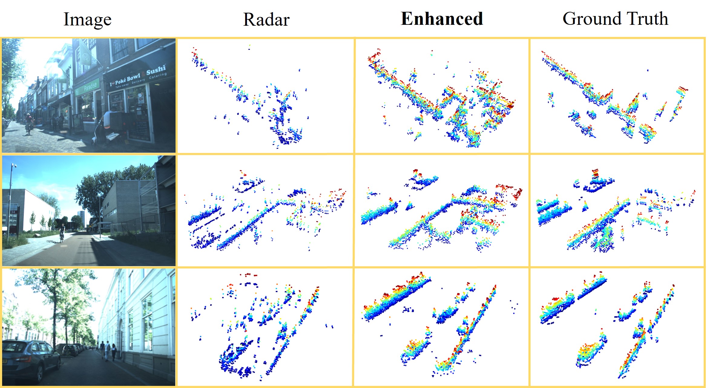
Figure 1: Enhancement effect of our method on radar point clouds. The image, raw radar points, enhanced point clouds, and LiDAR point clouds of the corresponding scene are shown in the figure.

Recently, diffusion-based approach, denoising diffusion probabilistic model (DDPM) [10], has demonstrated superior performance on image super-resolution [20] and video restoration [24]. It generates high-quality super-resolved images by progressively denoising the degraded input image, making the model particularly suited for high-noise scenarios. However, applying the diffusion model to sparse radar point clouds is still relatively unexplored and challenging.

In this paper, we employ the idea of DDPM and propose a novel Radar-diffusion for radar point clouds super-resolution, as shown in Fig. 1. Our approach begins by transforming the radar point clouds into bird’s eye view (BEV) images and then supervised using the corresponding LiDAR BEVs. During training, we use a diffusion model based on mean-reverting stochastic differential equations (SDEs) to process LiDAR BEV images, simulating the transition from denser LiDAR data to radar data using our devised objective function. After training, the model reverse denoising enhances input radar BEV images, producing LiDAR-like, denser results for accurate super-resolution. We demonstrate that our approach achieves state-of-the-art results in point cloud super-resolution and exhibits robust generalization capabilities to unseen scenarios. Furthermore, we assess the performance of the generated high-resolution point cloud in the downstream registration task [21, 23]. The results show that the enhanced point cloud can be well used for downstream tasks, revealing its potential for all-weather perception applications.

In summary, our work makes three main contributions:

• Proposal of Radar-diffusion as the first approach to employ the modified diffusion model for achieving dense 3D radar point cloud super-resolution;

• Demonstration of the superior performance of the proposed Radar-diffusion incorporating our novel objective function in 3D radar point cloud super-resolution;

• Validation of the usability of the enhanced point clouds for downstream registration tasks.

II Related Work

The sparsity and high noise-to-signal ratio of radar point clouds pose critical challenges hindering the development of mmWave radar technology. Existing approaches for improving the quality of radar point clouds can be categorized into the pre-processing methods and the post-processing methods.

Zhang et al. [25] and Cho et al. [7] propose to replace traditional methods like fast Fourier transform during the signal processing with innovative algorithms [25] or learning-based algorithms [7]. CFAR [18] is a most commonly employed pre-processing approach. While effectively removing clutter points, CFAR also filters out lots of real detection points, resulting in extremely sparse radar point clouds. The learning-based method [2] has been proposed as an alternative to the CFAR process, directly operating on range-Doppler images for subsequent tasks. However, these methods require handling a large amount of data, placing high demands on system bandwidth and computational power. Gall et al. [8] employ neural networks to estimate the arrival direction of mmWave radar acquisition data, improving the accuracy and enhancing the resolution of acquired point clouds. Cheng et al. [6] propose a radar point detector network for high-quality point cloud extraction incorporating a spatiotemporal filter to handle clutter points. However, due to the nature of mmWave radar, target points and clutter points are highly correlated. Introducing more radar detection inevitably causes more clutter points. Furthermore, the generated point clouds using pre-processing methods are still sparse.

Post-processing methods commonly employ the neural network for clutter point handling and super-resolution. Chamseddine et al. [3] utilize the PointNet [17] to distinguish the ghost targets and real targets, resulting in accurate radar point clouds. Guan et al. [9] effectively recover high-frequency object shapes from the original low-resolution radar point clouds in rainy and foggy weather conditions using a cGAN [14] architecture. Prabhakara et al. [16] propose the RadarHD employing an U-Net [19] to generate LiDAR-like dense point clouds from low-resolution radar point clouds. Our approach is also a post-processing approach. Unlike existing methods that focus on single-object super-resolution [9] or 2D radar point cloud super-resolution [16], our approach addresses 3D radar point cloud super-resolution within the context of autonomous driving scenes. To the best of our knowledge, this is the first approach addressing 3D radar point cloud super-resolution using diffusion model.

\begin{overpic}[width=429.28616pt]{pics/pipeline24.jpg} \put(27.2,20.8){{\scriptsize{$x$}}} \put(26.8,1.3){{\scriptsize{$\mu$}}} \put(40.5,17.2){{\scriptsize{$x(0)$}}} \put(57.2,17.2){{\scriptsize{$x(T)$}}} \put(67.2,17.2){{\scriptsize{$x(T)$}}} \put(95.7,17.2){{\scriptsize{$\tilde{x}(0)$}}} \put(85.5,22.6){{\scriptsize{$\tilde{x}(t-1)$}}} \put(57.6,30.2){{\scriptsize{$\times T$}}} \put(93.8,30.2){{\scriptsize{$\times T$}}} \put(55.9,10.0){{\scriptsize{$\times T$}}} \put(81.6,9.8){{\scriptsize{$\times T$}}} \par\end{overpic}

Figure 2: Training process and generating process of our proposed Radar-diffusion. The training process models the degradation of LiDAR BEV image to radar BEV image as the forward diffusion process defined by mean-reverting SDE. By learning the reverse denoising process, the LiDAR-like BEV image is then recovered.

III Our approach

We propose Radar-diffusion to enhance sparse mmWave radar point clouds to generate dense LiDAR-like point clouds useful for downstream tasks. The overview of our method is illustrated in Fig. 2. We begin with converting the radar and LiDAR point clouds into BEV images. Subsequently, we model the degradation of high-quality LiDAR BEV images to low-quality radar BEV images using the forward diffusion process of mean-reverting SDE. By learning the corresponding reverse denoising process using our proposed objective function, high-quality LiDAR-like BEV images are then recovered. Note that no LiDAR data is required during the generating process.

III-A Data Processing

To enable network processing and learning across different sensory modalities, we first convert LiDAR and radar point clouds into BEV images and extract their shared field of view (FOV). The overview of the data processing is illustrated in Fig. 3.

Ground point removal. We first remove ground points from the raw point cloud data, as they lack valuable semantic information and may hinder the super-resolution learning process. Furthermore, radar point clouds usually contain few ground points due to the limited resolution of radar echo intensity, so no additional steps are required for their removal. For the LiDAR data, we utilize the Patchwork++ [11] to detect and remove the ground points from the LiDAR point cloud. It uses adaptive ground likelihood estimation to iteratively approximate the ground segmentation region, ensuring correct separation of ground point clouds even when the ground is elevated by different layers.

Shared field of view extraction. We then align the LiDAR point $(x_{l},y_{l},z_{l})$ to the radar coordinate system by

$$\begin{bmatrix}x_{c}&y_{c}&z_{c}&1\end{bmatrix}^{\top}=\begin{bmatrix}\textbf{R}^{r}_{l}&\textbf{t}^{r}_{l}\\ 0&1\end{bmatrix}\begin{bmatrix}x_{l}&y_{l}&z_{l}&1\end{bmatrix}^{\top},$$ (1)

where $\textbf{R}^{r}_{l}$ and $\textbf{t}^{r}_{l}$ refer to the rotation and translation matrix from the radar to the LiDAR coordinate system. As we intend to use the BEV image to represent the point cloud, we simplify the shared FOV extraction by focusing solely on their shared horizontal FOV. We use a Velodyne HDL-64 S3 LiDAR with a horizontal FOV of $360^{\circ}$ and a FRGen21 radar with a horizontal FOV of $120^{\circ}$. By calculating point yaw angles ($\theta$), we retain LiDAR points and radar points whose yaw angles satisfy $\theta\in[30^{\circ},150^{\circ}]$.

BEV generation: We transform the LiDAR and radar point clouds into compact BEV images with channel information representing height. This facilitates fast and efficient feature learning using mature visual methods. On the other hand, BEV images can better present overall scenes, enabling parallel completion of various perception tasks. To create these BEV images, we retain the points with $x$ coordinates within the range of $[-15,15]$, $y$ within the range of $[0,30]$, and $z$ within the range of $[-0.8,1.7]$. Subsequently, we compress these points into a $256\times 256$ BEV image with a resolution of $30/256$ m. The grayscale value $G_{i,j}$ for each pixel $\{i,j\}$ is determined based on the $z$ value of the highest point falls within that pixel

$$G_{i,j}=[\max(P_{i,j}*\begin{bmatrix}0&0&1\end{bmatrix}^{\top})-\gamma]_{+}/{\text{range}_{z}}*255,$$ (2)

where $[\bullet]_{+}=\max(\bullet,0)$, $P_{i,j}$ represents the point set falls within pixel $\{i,j\}$, and $\gamma$ is a predefined threshold.

Multi-frame input: Given the sparse nature of the radar point cloud, we combine data from multiple consecutive radar frames using their relative poses. In practice, the relative poses can be obtained through the point cloud registration method [1, 22] or LiDAR odometry method [4]. We utilize BEV images generated from the aggregated radar point cloud from $5$ consecutive frames as network input.

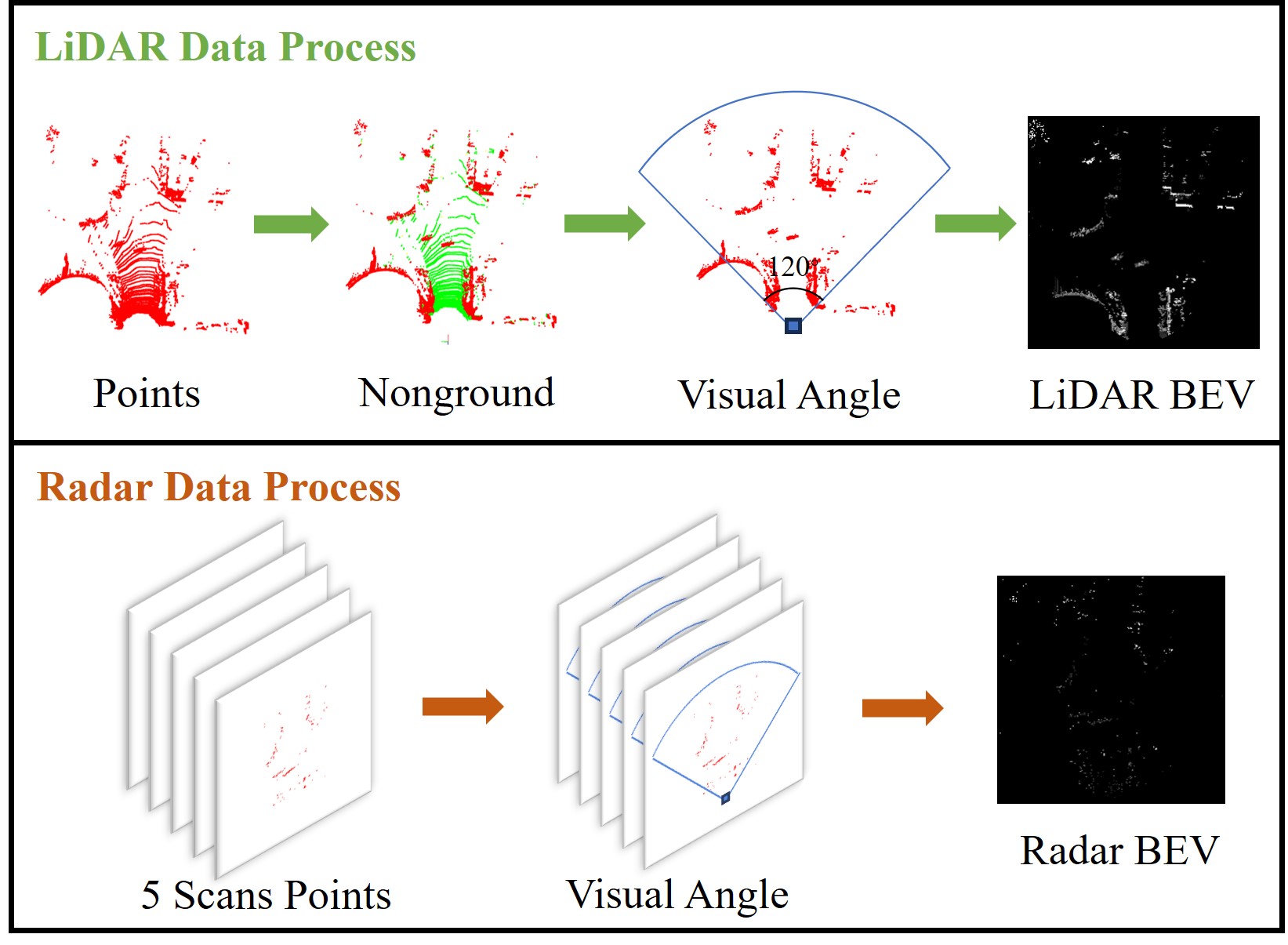
Figure 3: The data process of LiDAR and radar point clouds.

III-B Forward Process based on the Mean-Reverting SDE

The standard diffusion process defined by SDE follows

$$\mathrm{d}x=f({x},t)\mathrm{d}t+g({t})\mathrm{d}w,\quad x(0)\sim p_{0}(x),$$ (3)

where $x$ refers to the state linked to LiDAR BEV image, ${f}({x},t)$ and ${g}({t})$ are drift and dispersion functions, and $w$ is a standard Brownian motion. Typically, this leads to a terminate state $x(T)$ following a Gaussian distribution with zero mean and fixed variance. Unlike standard SDE widely applied in vision tasks, adding random Gaussian noise to $x$. To model the degradation of the LiDAR BEV image to the radar BEV image, we employ mean-reverting SDE that includes autoregressive Ornstein-Uhlenbeck noise (OU noise) [12] leading to a final state with biased mean and variance. This modification aligns with our objective of matching radar data to LiDAR data, teaching the model how to super-resolve radar data during inference. This forward process can be formulated as

$$\mathrm{d}x=\theta_{t}\left(\mu-x\right)\mathrm{d}t+\sigma_{t}\mathrm{d}w,\quad x(0)\sim p_{0}(x),$$ (4)

where $\mu$ is the state mean of the radar BEV image, $\theta_{t}$ characterizes the speed of mean reversion, $\sigma_{t}$ is the diffusion coefficient. By setting $\sigma_{t}^{2}/\theta_{t}=2\lambda^{2}$, where $\lambda^{2}$ is the stationary variance, we derive the distribution of $x(t)$ as

$$p_{t}(x) =\mathcal{N}\big{(}x(t)\mid m_{t}(x),v_{t}\big{)},$$ (5)

$$m_{t}(x): =\mu+\left(x(0)-\mu\right)\mathrm{e}^{-\bar{\theta_{t}}},$$ (6)

$$v_{t}: =\lambda^{2}\left(1-\mathrm{e}^{-2\bar{\theta_{t}}}\right),$$ (7)

$$\bar{\theta_{t}}: =\int_{0}^{t}{\theta_{z}}\mathrm{d}z,$$ (8)

where the mean state $m_{t}$ and the variance $v_{t}$ converge to $\mu$ and $\lambda^{2}$ respectively as $t\to\infty$. This implies that by progressively adding OU noise, the terminate state of LiDAR BEV image $x(T)$ converges to the radar BEV image $\mu$ with fixed Gaussian noise $\mathcal{N}(0,\lambda)$.

III-C Denoising Process on the Mean-Reverting SDE

To recover the LiDAR-like BEV image, we reverse the process of mean-reverting SDE by

$$\mathrm{d}\tilde{x}=\left[\theta_{t}-\sigma_{t}^{2}\nabla_{\tilde{x}}\log p_{t}(\tilde{x})\right]\mathrm{d}t+\sigma_{t}\mathrm{d}w,\,\tilde{x}(T)=x(T),$$ (9)

where $\nabla\log p_{t}(\tilde{x})$ is the score function learned by the time-dependent U-Net [10].

Specifically, according to Eq. (5), we can obtain the ground truth of $\nabla\log p_{t}(\tilde{x})$ as

$$\nabla_{\tilde{x}}\log p_{t}(\tilde{x})=-\frac{\tilde{x}(t)-m_{t}}{v_{t}}.$$ (10)

By rewriting $\tilde{x}(t)=m_{t}(\tilde{x})+\sqrt{v_{t}}\epsilon_{t}$, where $\epsilon_{t}\sim\mathcal{N}(0,I)$ is the standard Gaussian noise, we further derive Eq. (10) as

$$\nabla_{\tilde{x}}\log p_{t}(\tilde{x}) =-\frac{\epsilon_{t}}{\sqrt{v_{t}}}.$$ (11)

The neural network predicts the noise $\tilde{\epsilon}(\tilde{x}(t),\mu,t)$ based on current state $\tilde{x}(t)$, condition $\mu$, and time $t$.

III-D Objective Function

Instead of using the standard objective that supervises the network to learn the accurate noise, we follow Luo et al. [13] and train the U-Net to recover more accurate reversed images by minimizing image residuals at the same stages between forward and denoising processes using the following objective function

$$J(\tilde{\epsilon}): =\sum_{i=1}^{T}\gamma_{i}\mathbb{E}\Big{[}\|\underbrace{\tilde{x}(i)-(\mathrm{d}\tilde{x}(i))_{\tilde{\epsilon}}}_{\mathrm{reversed~{}}x(i-1)}-x(i-1)\|\Big{]},$$ (12)

$$=\sum_{i=1}^{T}\gamma_{i}\mathbb{E}[\|\tilde{x}(i-1)-x(i-1)\|],$$

where $\gamma_{i}$ represents positive weight, $(\mathrm{d}\tilde{x}(i)_{\tilde{\epsilon}}$ represents the mean-reverting SDE defined in Eq. (9) using the score $-\tilde{\epsilon}/\sqrt{v_{t}}$ learned by the network, and $x(i-1)$ is the ideal state for reversed $\tilde{x}(i)$, i.e., the state at time $t=i-1$ in the diffusion process. This objective function exploits the cumulative error within the denoising process, achieving more stable training for image generation tasks.

However, unlike the visual image generation task, LiDAR and radar BEV images’ data distribution is significantly imbalanced. We observe that the blank area in LiDAR BEV image commonly approximates 20 times larger than the area with actual sensor detection. Equivalently learning the overall reverse image leads the network to utilize a conservative strategy that simply sets every confused area to blank. Therefore, we propose dividing the objective function into two parts, considering the blank area and the actual detection area separately. To this end, we calculate mask matrix ${\mbox{{{M\/}}}}=\llbracket x(0)>0\rrbracket$ and $\bar{{\mbox{{{M\/}}}}}=\llbracket x(0)==0\rrbracket$, where $\llbracket\bullet\rrbracket$ is an indicator function for which the statement is true. The modified objective function is written as

$$J =J_{\text{target}}+w\times J_{\text{blank}},$$ (13)

$$J_{\text{target}} =\sum_{i=1}^{T}\gamma_{i}\mathbb{E}[\|{\mbox{{{M\/}}}}\odot\tilde{x}(i-1)-{\mbox{{{M\/}}}}\odot x(i-1)\|],$$

$$J_{\text{blank}} =\sum_{i=1}^{T}\gamma_{i}\mathbb{E}[\|\bar{{\mbox{{{M\/}}}}}\odot\tilde{x}(i-1)-\bar{{\mbox{{{M\/}}}}}\odot x(i-1)\|],$$

where $\odot$ represents the Hadamard product. Using our proposed objective function significantly improves the overall performance in our experiments.

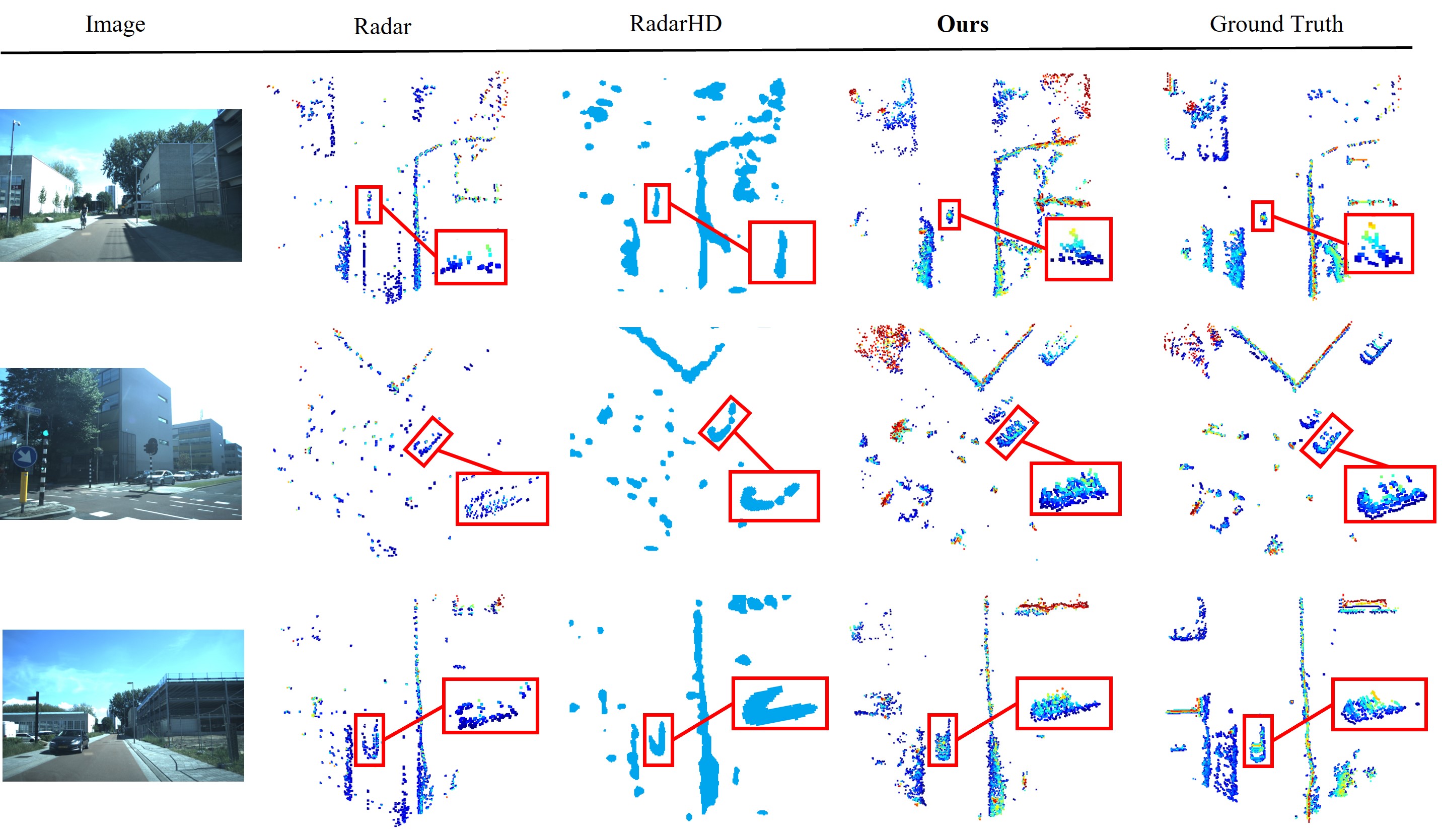
Figure 4: Qualitative results of our method and the RadarHD on the VOD dataset. Specifically, the point clouds enhanced by RadarHD are in 2D, while the point clouds enhanced by our method are in 3D.

IV Experimental Evaluation

IV-A Dataset

We train and evaluate our approach on View-of-Delft (VOD) dataset [15] and RadarHD dataset [16]. The VOD dataset contains 8,693 frames of data collected by a Velodyne HDL-64 LiDAR and a FRGen21 radar in complex urban traffic environments. The RadarHD dataset is collected in an indoor office environment utilizing Ouster OS0-64 LiDAR and AWR1843 radar without height dimension in the point cloud data. Our evaluating datasets cover both outdoor urban roads and indoor environments to test the robustness of different methods.

IV-B Implementation Details

We train our model using the Lion optimizer [5], with an initial learning rate of $4\times 10^{-5}$. We choose a more robust noise level $\sigma=50$ and $w=2$ for the forward diffusion process and objective function, respectively. $\gamma_{i}=1$ is equivalent in all timesteps $t$. We train our model on a single NVIDIA RTX 4090 with a batch size of 8. Total training time takes 9 hours, and the .pth format model size is 306.7 MB.

IV-C Performance on Point Cloud Super-Resolution

We evaluate the point cloud super-resolution performance of our method on VOD and RadarHD datasets. For VOD dataset, we divide it into 7831 frames for training and 635 frames for testing. The test set contains new frames in unseen sequences, allowing for a comprehensive evaluation of the generalization ability. For RadarHD dataset, we adopt the setup of Prabhakara et al. [16], utilizing 28 trajectories with 22,784 frames for training and 39 distinct trajectories with 36,779 frames for testing. As the RadarHD dataset only contains 2D radar data, our approach designed for 3D radar point clouds is not directly applicable. Therefore, we employ the following modifications for training on RadarHD dataset. We set the grayscale of the input radar BEV image to the point intensity and the input LiDAR BEV image to $\{0,255\}$, indicating whether there is a point.

TABLE I: Super-resolution Performance.

VOD dataset
	FID${}_{\text{BEV}}\downarrow$	CD$\downarrow$	MHD$\downarrow$	UCD$\downarrow$	UMHD$\downarrow$
RadarHD	247.2	0.34	0.24	0.45	0.24
ours	118.4	0.19	0.10	0.15	0.07
RadarHD dataset
	FID${}_{\text{BEV}}\downarrow$	CD$\downarrow$	MHD$\downarrow$	UCD$\downarrow$	UMHD$\downarrow$
RadarHD	141.1	0.44	0.34	0.38	0.21
ours	139.0	0.59	0.50	0.26	0.13

• The best results are highlighted in bold. All metrics are in 2D.

Metrics: We employ the following metrics to evaluate the quality of the enhanced radar point cloud comparing to the LiDAR point cloud: (i) Fréchet Inception Distance (FID${}_{\text{BEV}}$), the Fréchet distance between the generated enhanced BEV images and LiDAR BEV images. (ii) Chamfer Distance (CD), the average distance from each point to the nearest neighbor point in the other point cloud. (iii) Modified Hausdorff Distance (MHD), the median distance from each point to the nearest neighbor point in the other point cloud. Given that radar possesses a stronger penetration ability, it can detect objects occluded in the LiDAR point clouds, potentially generating more informative point clouds than LiDAR. We thereby present two more metrics for better evaluation: (iv) Unidirectional Chamfer Distance (UCD), the CD from LiDAR point cloud to enhanced radar point cloud only, and (v) Unidirectional Modified Hausdorff Distance (UMHD), the MHD from LiDAR point cloud to enhanced radar point cloud only.

Results: Since radar point cloud super-resolution is a new research direction, no similar work currently achieves super-resolution on 3D radar point clouds. The only baseline we find is RadarHD [16] for 2D radar point cloud super-resolution. Thus, for a fair comparison, we conduct all metrics in 2D, i.e., using only $(x,y)$ coordinates, while providing 3D evaluation in our ablation study. We present experimental results as in Tab. I. As depicted on the VOD dataset, our approach produces superior results across all metrics, with an average improvement of 58.4 %. Notably, our approach exhibits significant advantages over RadarHD in terms of UCD and UMHD metrics, achieving a 64.7 % improvement in UCD and a 70.8 % improvement in UMHD. This can be attributed to our approach better faithfully reproduces the information presented in the LiDAR point cloud. On the RadarHD dataset, our approach maintains its advantages regarding FID, UCD, and UMHD metrics. However, compared to RadarHD, our approach exhibits certain decreases in the CD and MHD metrics. This is because our method can generate denser point clouds and even incorporate information that may not be present in the original LiDAR point cloud. However, the enriched points do not possess real correspondences in the LiDAR point cloud, thus introducing larger errors in CD and MHD metrics. The fact that our approach generates denser point clouds is demonstrated in the subsequent qualitative experiments.

To provide more insights into the proposed Radar-diffusion, we visualize the enhanced 3D radar point clouds using Radar-diffusion as in Fig. 4. As RadarHD is only capable of 2D radar point cloud generation, we visualize its generated BEV image for comparison. It can be observed that the point clouds enhanced by our method effectively capture the overall layout. We further zoom in on representative regions, such as vehicles and pedestrians, for closer examination. As depicted, our enhanced point clouds possess realistic geometric structures for objects while enriching their details that can be occluded in LiDAR point clouds.

IV-D Performance on Downstream Task: Registration

Our enhanced point clouds present a precise overall layout while possessing enriched details, making them capable of downstream tasks. In this experiment, we demonstrate the capability of our enhanced point cloud for downstream registration tasks. We evaluate our method on the test sets of the VOD dataset. The point cloud pairs with ground truth pose distances more than $1$ m are chosen as test samples.

Metrics: We employ three metrics to evaluate the registration performance: i) Relative Translation Error (RTE), which measures the Euclidean distance between estimated and ground truth translation vectors, ii) Relative Rotation Error (RRE), which is the average difference between estimated and ground truth rotation, and iii) Registration Recall (RR), representing the fraction of scan pairs with RRE and RTE below certain thresholds, e.g., 5^∘ and 0.5 m.

TABLE II: Registration Performance using Enhanced Point Cloud.

	RR(%)$\uparrow$	RTE(m)[succ./all]$\downarrow$	RRE(∘)[succ./all]$\downarrow$
Raw	88.51	0.11/0.52	0.48/2.39
Enhanced (ours)	93.10	0.11/0.22	0.61/1.13

• The best results are highlighted in bold.

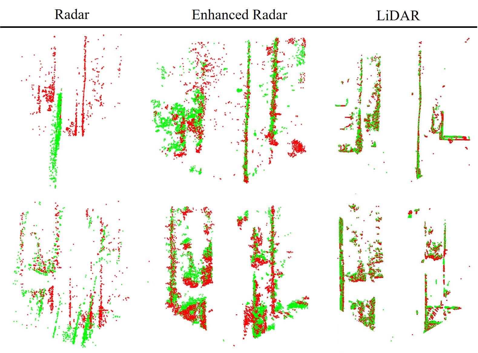
Figure 5: Qualitative results of registration on radar point clouds, our enhanced radar point clouds, and LiDAR point cloud using RDMNet [22]. Different colors represent different frames of point clouds.

Results: In Tab. II, we present registration results on raw radar point clouds and enhanced radar point clouds generated by our Radar-diffusion utilizing the state-of-the-art registration method, RDMNet [22]. It is a deep learning-based method that finds dense point matches over two point clouds and subsequently performs accurate registration. We directly apply it to different point cloud data to evaluate the registration performance. We adjust the correspondence number according to the point cloud density for a fair comparison. As depicted, our enhanced point clouds exhibit good consistency and accuracy for reliable registration. Furthermore, the more detailed information provided by our enhanced point clouds allows for more robust registration compared to radar point clouds. We visualize some registration results using different point clouds in Fig. 5. As can be seen, due to the sparse nature of the original radar data, the registration process failed to align two overlapping radar scans. In contrast, the enhanced radar data can be aligned as well as the registration results of the corresponding LiDAR point clouds.

IV-E Ablation Studies

We conduct ablation studies to demonstrate the effectiveness of our design in Tab. III. Firstly, we study the objective function. As shown, compared to the original objective function, using our proposed objective function significantly improves the performance across all metrics. Different choices of $w$ in Eq. (13) have different emphasis on the final performance of the network. A larger value of $w$ tends to encourage the network to adopt a more conservative approach, making it more inclined to generate unclear or ambiguous regions as blank. We use $w=2$ as the default as it achieves the most balance performance. Secondly, we study the number of input frames. As depicted, our approach can work with different numbers of inputs. Merging 5 frames of radar point cloud results in the best performance.

TABLE III: Ablation Study on the VOD-Dataset.

case	FID${}_{\text{BEV}}\downarrow$	CD$\downarrow$	MHD$\downarrow$	UCD$\downarrow$	UMHD$\downarrow$
original	165.4	1.42	1.72	2.39	1.72
$w=2$	118.4	0.64	0.45	0.52	0.32
$w=4$	103.9	0.68	0.45	0.73	0.42
$w=5$	116.7	0.65	0.45	0.51	0.32
1scans	130.1	0.72	0.52	0.54	0.33
3scans	122.1	0.67	0.47	0.50	0.31
5scans	118.4	0.64	0.45	0.52	0.32

• The best results are highlighted in bold.

• Besides FID${}_{\text{BEV}}$, other metrics are calculated in 3D.

V Conclusion

In this paper, we present a mean-reverting SDE-based diffusion model for 3D mmWave radar point cloud super-resolution. Our approach models the degradation of high-quality LiDAR BEV image to low-quality radar BEV image as the forward diffusion process, and then learns the reverse process to recover high-quality LiDAR-like BEV images. We propose to improve the object function to make it more suitable for radar super-resolution tasks. Experiments show that our method can gently handle the massive clutter points in radar point clouds while enhancing them into high-quality LiDAR-like point clouds. Additionally, we demonstrate that our enhanced point clouds can be effectively utilized for downstream registration tasks, laying the foundation for future all-weather perception applications.

References

- [1] P. Besl and N. McKay. A Method for Registration of 3D Shapes. IEEE Trans. on Pattern Analysis and Machine Intelligence (TPAMI), 14(2):239–256, 1992.
- [2] D. Brodeski, I. Bilik, and R. Giryes. Deep radar detector. In 2019 IEEE Radar Conference (RadarConf), pages 1–6. IEEE, 2019.
- [3] M. Chamseddine, J. Rambach, D. Stricker, and O. Wasenmuller. Ghost target detection in 3d radar data using point cloud based deep neural network. In Proc. of the Intl. Conf. on Pattern Recognition (ICPR), pages 10398–10403. IEEE, 2021.
- [4] X. Chen, A. Milioto, E. Palazzolo, P. Giguère, J. Behley, and C. Stachniss. SuMa++: Efficient LiDAR-based Semantic SLAM. In Proc. of the IEEE/RSJ Intl. Conf. on Intelligent Robots and Systems (IROS), 2019.
- [5] X. Chen, C. Liang, D. Huang, E. Real, K. Wang, Y. Liu, H. Pham, X. Dong, T. Luong, C.J. Hsieh, et al. Symbolic discovery of optimization algorithms. arXiv preprint, 2023.
- [6] Y. Cheng, J. Su, M. Jiang, and Y. Liu. A novel radar point cloud generation method for robot environment perception. IEEE Trans. on Robotics (TRO), 38(6):3754–3773, 2022.
- [7] H.W. Cho, W. Kim, S. Choi, M. Eo, S. Khang, and J. Kim. Guided generative adversarial network for super resolution of imaging radar. In 2020 17th European Radar Conference (EuRAD), pages 144–147. IEEE, 2021.
- [8] M. Gall, M. Gardill, T. Horn, and J. Fuchs. Spectrum-based single-snapshot super-resolution direction-of-arrival estimation using deep learning. In 2020 German Microwave Conference (GeMiC), pages 184–187. IEEE, 2020.
- [9] J. Guan, S. Madani, S. Jog, S. Gupta, and H. Hassanieh. Through fog high-resolution imaging using millimeter wave radar. In Proc. of the IEEE/CVF Conf. on Computer Vision and Pattern Recognition (CVPR), pages 11464–11473, 2020.
- [10] J. Ho, A. Jain, and P. Abbeel. Denoising diffusion probabilistic models. Proc. of the Advances in Neural Information Processing Systems (NIPS), 33:6840–6851, 2020.
- [11] S. Lee, H. Lim, and H. Myung. Patchwork++: Fast and robust ground segmentation solving partial under-segmentation using 3d point cloud. In Proc. of the IEEE/RSJ Intl. Conf. on Intelligent Robots and Systems (IROS), pages 13276–13283. IEEE, 2022.
- [12] T.P. Lillicrap, J.J. Hunt, A. Pritzel, N. Heess, T. Erez, Y. Tassa, D. Silver, and D. Wierstra. Continuous control with deep reinforcement learning. arXiv preprint, 2015.
- [13] Z. Luo, F.K. Gustafsson, Z. Zhao, J. Sjölund, and T.B. Schön. Image restoration with mean-reverting stochastic differential equations. arXiv preprint, 2023.
- [14] M. Mirza and S. Osindero. Conditional generative adversarial nets. arXiv preprint, 2014.
- [15] A. Palffy, E. Pool, S. Baratam, J.F. Kooij, and D.M. Gavrila. Multi-class road user detection with 3+ 1d radar in the view-of-delft dataset. IEEE Robotics and Automation Letters (RA-L), 7:4961–4968, 2022.
- [16] A. Prabhakara, T. Jin, A. Das, G. Bhatt, L. Kumari, E. Soltanaghai, J. Bilmes, S. Kumar, and A. Rowe. High resolution point clouds from mmwave radar. In Proc. of the IEEE Intl. Conf. on Robotics & Automation (ICRA), pages 4135–4142. IEEE, 2023.
- [17] C.R. Qi, H. Su, K. Mo, and L.J. Guibas. PointNet: Deep Learning on Point Sets for 3D Classification and Segmentation. In Proc. of the IEEE Conf. on Computer Vision and Pattern Recognition (CVPR), 2017.
- [18] M.A. Richards. Fundamentals of radar signal processing. McGraw-Hill Education, 2022.
- [19] O. Ronneberger, P. Fischer, and T. Brox. U-net: Convolutional networks for biomedical image segmentation. In Medical Image Computing and Computer-Assisted Intervention–MICCAI 2015: 18th International Conference, Munich, Germany, October 5-9, 2015, Proceedings, Part III 18, pages 234–241. Springer, 2015.
- [20] C. Saharia, W. Chan, H. Chang, C. Lee, J. Ho, T. Salimans, D. Fleet, and M. Norouzi. Palette: Image-to-image diffusion models. In ACM SIGGRAPH 2022 Conference Proceedings, pages 1–10, 2022.
- [21] C. Shi, X. Chen, K. Huang, J. Xiao, H. Lu, and C. Stachniss. Keypoint Matching for Point Cloud Registration using Multiplex Dynamic Graph Attention Networks. IEEE Robotics and Automation Letters (RA-L), 6:8221–8228, 2021.
- [22] C. Shi, X. Chen, H. Lu, W. Deng, J. Xiao, and B. Dai. Rdmnet: Reliable dense matching based point cloud registration for autonomous driving. IEEE Trans. on Intelligent Transportation Systems (T-ITS), 2023.
- [23] C. Shi, X. Chen, J. Xiao, B. Dai, and H. Lu. Fast and accurate deep loop closing and relocalization for reliable lidar slam. arXiv preprint, 2023.
- [24] V. Voleti, A. Jolicoeur-Martineau, and C. Pal. Mcvd-masked conditional video diffusion for prediction, generation, and interpolation. Proc. of the Advances in Neural Information Processing Systems (NIPS), 35:23371–23385, 2022.
- [25] F. Zhang, C. Wu, B. Wang, and K.R. Liu. mmeye: Super-resolution millimeter wave imaging. IEEE Internet of Things Journal, 8(8):6995–7008, 2020.