First-Order Vortex Lattice Melting in Bilayer Ice: A Monte Carlo Method Study

Abstract

Inspired by the stable bilayer water ice grown in the laboratory (Nature 577, 60, 2020), we propose a model representing water ice as a two-layer six-vertex model. Using the loop update Monte Carlo method, we unveil meaningful findings. While the square lattice six-vertex model exhibits an antiferromagnetic to disordered phase transition known as the Berezinskii-Kosterlitz-Thouless transition, we observe a different scenario for the bilayer six-vertex model, where the transition type transforms into an Ising transition. We discover the emergence of vortices in the disordered phase, and to stabilize them, vortex excitation is induced. This leads to the presence of distinct 1/2 filling and 2/3 filling vortex lattice phases. Importantly, we identify the phase transitions between the vortex lattice phase and the disorder phase, as well as between the 1/2 and 2/3 vortex lattices, as being of first order. Our findings provide valuable insights into the nature of phase transitions occurring in layered water ice and artificial spin ice systems in experimental setups.

I introduction

Ice is a common substance in nature. There are various types of ice, including the solid form of liquid water [1], spin ice in real materials [2], and artificial spin ice [3, 4]. One common feature of the different forms of ice is the ice rule, i.e., the so called two-in (close) two-out (far away) topological constraint, introduced by Pauling in 1935 [5]. Water ice exhibits 19 stable geometric structures, currently identified through high pressure and low temperature experiments [1]. Spin ice also exists in a lot to real materials with different structures, such as rare-earth pyrochlores $\text{Ho}_{2}\text{Ti}_{2}\text{O}_{7}$ [6].

Researchers have also attempted to grow artificial spin ices  [7], due to their controllability. The microscale systems used to create artificial spin ice typically involve magnetically interacting nanoislands or nanowire links[8], superconducting-qubit arrays [9].The physics studied through ice are very wide, such as residual entropy  [10], frustration [2], monopoles [11] and so on.

Artificial spin ice can construct various configurations, including vortex lattice (VL) phase [12]. The periodic structure composed of vortices is called the VL. As vortex states can help understand superconductors [13], a lot of studies have been done on transitions between vortex lattices and other phases [14, 15, 16, 17]. In the XY model, the unbinding of vortex-antivortex pairs is considered the cause of Berezinskii-Kosterlitz-Thouless (BKT) phase transition [18, 19, 20]. However, the vortex lattice leads to a first-order phase transition in real crystals YBCO and $\text{YBa}_{2}\text{Cu}_{3}\text{O}_{7}$  [14, 15, 16, 17].

Of course, the ice physics can also be explored through experiments with water ice. In 2020, the group at Peking University has confirmed the existence of two-dimensional two-layered water ice [21]. The positions of the upper layer oxygen ions, as well as the connections between the oxygen ions, are exactly the same as those in the lower layer, i.e., AA stacking ice. Such stable structure of water was first predicted in 1997 using molecular dynamics simulation [22]. Actually, there exists another type of ice with an AB stacking structure [23] as shown Fig. 1. There is a relative 180 degree rotation between the two layers, which are connected by hydrogen bonds. Alternatively, the hydrogen bonds of the first layer are shifted onto the faces of the second layer. It has been confirmed to be stable under reasonable temperature and pressure by first-principles calculations [23] but lack of experimental preparation [21].

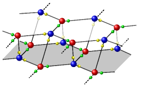
Figure 1: The construction of the two-layer ice model. The large balls (in red and blue) represent $O^{2-}$s and the small balls denote $H^{+}$s. The different colors for the large ball means AB stacking [23]. The two-in-two-out rule can be demonstrated by the small balls in different colors.

To inspire experimental physicists to achieve AB or other type of bilayer ice in the future, we further convert bilayer ice to bilayer six-vertex (6V) model model [24]. On the basis of the bilayer square lattice 6V model, the AB stacking honeycomb 6V model can be formed by bending one leg of the vertexes to the appropriately. Hydrogen ions and oxygen ions in ice can be close or far apart, similar to spin-up and spin-down. Viewing ice as a spin system helps understand the phase transitions between different types of ice under various conditions like temperature and pressure. It is not clear that whether or not there are something new in the bilayer honeycomb 6V model.

In this paper, we apply a large-scale loop Monte Carlo (MC) simulation to study the proposed 6V model. By properly defining and scanning the type and weight, including the vortex-exciting weight, we explore the phase diagram systematically. The system includes ferromagnetic, antiferromagnetic, 1/2-filling VL, 2/3-filling VL, and disordered phases. The theoretically discovered types of phase transitions, such as first-order phase transitions, also provides insights into understanding previous experiments [14, 15, 16, 17].

The outline of this work is as follows. Sec. II introduces the bilayer 6V model, algorithm, and the measured quantities. Sec. III describes the phase diagram and details without the effects of vortex weight $V=1$. Sec. IV describes the phase diagram with the effects of vortex weight $V\neq 1$. Conclusive comments and outlook are made in Sec. V.

Physically, apart from the bilayer 6V model initially propose, we have made new discoveries as follows:

(I) The transition between the antiferromagnetic phase to the disordered phase is the Ising type for our bilayer 6V model. However, for the 6V model on the square lattice, the transition is the BKT type [25].

(II) Two types of vortex lattice phase is found when vortex excitation is induced. The transition from vortex lattice phases to other phases is of first order, consistent with previous crystal experiments [14, 15] . It helps researchers understand that not all phase transitions involving vortices are BKT phase transitions.

On the algorithmic level, although Ref. [24] has simulated the single-layer planar 6V model using loop algorithm, the model here is the non-planar 6V model and we provide the details of closing loops. In addition, we introduce a Metropolis-type of short-loop update method for the purpose of ergodicity.

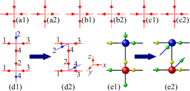
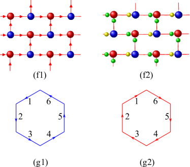
Figure 2: Schematic diagram of the 6V model and water molecules. (a1)-(c2) The configurations of six vertices and their weights defined as $a$, $a$, $b$, $b$, $c$ and $c$, respectively. (d1)-(d2) Connecting the two vertices by the two vertical red legs marked by 2 and 4. (e1)-(e2) Rotating the two legs, blue respectively, on the horizontal plane. (f1)-(f2) Mapping to the structure of real water ice molecules. The small ball represents hydrogen ion and the large ball represents oxygen ion. (g1)-(g2) The definition of vortex.

II Model, algorithm and quantities

II.1 The 6V model with vortex weight

II.1.1 Hamilton and partition function

Unlike the models such as the Ising [26], XY [18, 19, 20], Potts  [27] models or the coupled spins such Ising-XY model [28], etc., the famous 6V model does not have a explicit Hamiltonian. But each type of vertex has its own weight and can also have an equivalent energy, and the vertex satisfies the two-in-two-out topological constraints. For convenience, to measure physical quantities related to specific heat and other energy-related quantities, a quasi-Hamiltonian is introduced as

$$\mathcal{H}=-\sum_{i=1}^{2N}\epsilon_{i}-v\sum_{j=1}^{2f}n_{i},$$ (1)

where $\epsilon_{i}$ is the effective energy for each vertex labeled by $i$, and $v$ is a local vortex energy for each plaquette. $n_{i}$ represents the number of vortices in each plaquette, where $n_{i}=1$ denotes a clockwise $\circlearrowright$ or a counterclockwise $\circlearrowleft$ vortex, and $n_{i}=0$ signifies the absence of a vortex. $N$ is the total number of vertex of one layer and $f$ is total faces of the honeycomb lattice of one layer.

Using the Boltzmann weight factor, the vertex weight is

$$\omega_{i}=\text{exp}(\beta\epsilon_{i})$$ (2)

and the vortex weight is

$$V_{i}=\text{exp}(\beta vn_{i})$$ (3)

where $\beta=1/k_{B}T$ is the inverse temperature and set to 1, and the partition function of the system is defined as follows

$$\mathcal{Z}=\prod_{i=1}^{2N}\omega_{i}\prod_{j=1}^{2f}V_{j}.$$ (4)

Figures 2 (a1)-(c2) show the configurations of six vertexes, and each vertex has four legs marked by the red arrows. The directions of the legs satisfy two facing out away from the center and two legs pointing toward the center. For simplicity, the weights of the six vertexes take values as

$$w_{i}=[a,a,b,b,c,c]$$ (5)

here the flipping symmetry of the leg direction is considered, i.e., the state of (a1) can be obtained by flipping the directions of the four legs of (a2), and therefore the weights of these two vertexes are the same as $a$. Totally, only three possible weight values $a$, $b$ and $c$ are needed for the six different configurations. This tradition is also used in Ref. [25].

It should be note that the vortex is defined as shown in Figs. 2 (g1) and (g2). Numerically, the requirement is that the angle difference between adjacent vectors is $\frac{\pi}{3}$, i.e.,

$$\theta_{\text{mod \{i,6\}+1 }}-\theta_{i}=\pi/3,$$ (6)

where $i$ ranges from 1 to 6. This type of definition does not need the saw function in Ref. [28] and is the same the one in Ref. [29].

II.1.2 The formation of two-layer honeycomb lattice structure

Figures 2(d1)-(e2) show how to use the vertexes to construct a two-layer honeycomb lattices. Firstly, 6V models are usually constructed in the two-dimensional plane, and it is rare to see two-layer 6V models. Here, the interlayer coupling is realized by connecting the two vertices, using the two red legs marked 2, 4 in the vertical direction. Then, the second step is rotating the two legs in blue to the horizontal $y$-direction. A small coordinate axes $x$, $y$, $z$ are shown for reference.

It is also essential to illustrate the relationship between the two-layer honeycomb 6V model and the structure of ordered water molecules. In Figs. 2(f1)-(f2), the arrows pointing towards the center of the vertex means, the approaching of the hydrogen (H) ions to the oxygen (O) ion in a real water molecule. Conversely, arrows pointing away from the center indicate that the hydrogen ions stays away from the oxygen ion. Ultimately, the arrangement of vertices can describe the structure of real water ice molecules.

In addition, the configurations of the system also depends the topological constraints of “two-in and two-out” rules [24, 30]. In other words, the arrows in the vertices have two pointing to the center and the other two back to the center. The real configurations of large lattices needs to be simulated by various MC methods [31, 32], which we will discussed in next section.

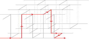
Figure 3: Schematic diagram of the loop algorithm in a two-layer honeycomb lattice. The start point is selected randomly, and the red arrows illustrate the path of the process. When the head of the loop meet the start vertex, the loop is closed and the configuration is updated. For convenience in defining the coordinates of the vertices, the honeycomb is defined as a topologically equivalent brick wall structure.

II.2 Methods and the measured quantities

II.2.1 Methods

In this paper, we apply the loop algorithm, which has has proven effective in studying various systems both classical systems systems [24], and quantum systems [33, 34]. A similar loop algorithm is the famous worm algorithm [35, 36], which involves a partial loop with two open ends with very efficient dynamical behaviours [37]. The 6V model is very similar to the flow representation of other models [38, 39, 40].

To execute a loop update, the following steps are performed:

1. First, we initialize the system with $N=2L_{x}\times L_{y}$ vertices, and then randomly select one of the vertices. Next, we randomly choose one of the four legs of the vertex to place the head of the loop.

2. The leg where the head of the loop is located is used as the entrance leg, and then again one of the four legs from that vertex is chosen as the exit leg with a certain probability.

3. The head of the loop enters the next new vertex, and the exit leg of the previous vertex is connected to this new vertex.

4. To continue the process, we repeat steps 2 and 3 until the head of the loop and the end of the loop meet. Additionally, as the head of the loop traverses each leg, the state (arrows) of that leg should be flipped.

Let us explain how the probability of selecting the exit leg when the loop head is determined. Here, we employ the Metropolis-Hastings strategy. Suppose the weight of the reference vertex is $w_{0}$, and the weights of the new vertices resulting from exiting from the four legs are $w_{1}$, $w_{2}$, $w_{3}$, and $w_{4}$ respectively. We choose a random number between 0 and 1 to determine the interval in which the random number falls. These intervals are defined as $[0,p_{1}]$, $(p_{1},p_{1}+p_{2}]$, $(p_{1}+p_{2},p_{1}+p_{2}+p_{3}]$, and $(p_{1}+p_{2}+p_{3},1]$, where the probabilities are defined as:

$$p_{i}=w_{i}/\sum_{i=1}^{4}w_{i}.$$ (7)

If the outgoing and incoming legs are exactly the same, then there is no update, and the corresponding probability $p$ is referred to as the bounce probability. Generally, a higher bounce probability leads to lower efficiency of the cluster algorithm [33, 34].

Therefore, analyzing the possible range of bounce probability under different parameters (see Table 1) here would be helpful to ensure the feasibility of the code.

$a+b$	$~{}\left|a-b\right|~{}$	$c$	$p_{a}$	$p_{b}$	$p_{c}$
$<1$	$\setminus$	$1$	$(0,\frac{1}{2})$	$(0,\frac{1}{2})$	$(\frac{1}{2},1)$
$\setminus$	$>1$	$1$	$(0,\frac{a}{a+1})$	$(0,\frac{b}{b+1})$	$(\frac{1}{a+b+1},\frac{1}{2})$

Table 1: Parameters $a$, $b$, and $c$, and the possible range of bounce probability $p_{a}$, $p_{b}$ and $p_{c}$, where the subscripts $a$, $b$, $c$ represent the vertices of type $a$, $b$, $c$ that the loop encounters during its walk.

Loop close is an important step in the loop algorithm. In some cases, the length of the loop is very big and the code consumes very long runtimes. Ref. [41] even cut the loop by the so-called short-loop mehtods.

Here, we resort to the method dealing with the quantum Bose-Hubbard models [42, 43, 44, 45], two ways of closing loops are used. In Fig. 4 (a), the beginning leg labeled by “first”, the ending leg is marked by “last”. In this case, the first and the last legs meet (overlap) at the same leg, and then the loop close. In Fig. 4 (b), the last leg connects to the position of the initial let. This constraint arises from the “2-in and 2-out” condition, allowing the loop closure only when connected to the initial leg. The distinction lies in the fact that in the former case, the vertex labeled “1” undergoes two updates, whereas in the latter, it undergoes only one time of update.

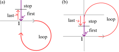
Figure 4: The two ways in which the loops close. (a) First and the last leg overlap at the same leg, and (b) the last leg connecting the first leg but the two leg belong to a pair of neighborhood Vertexes.

II.2.2 The measured quantities

(Ia) The magnetization in the $x$ direction,

$$M^{\pm}_{x}=\sum_{i,j}(\pm 1)^{i+j}S_{i,j}^{x}/N,$$ (8)

where $(\pm 1)$ mean the factor of phase of ferro-magnetization (FM) or antiferro-magnetization (AFM) respectively. The symbols $x$ refer to the horizontal directions of the lattice, and $i$ and $j$ means the coordinates of the vertices in the $x$ and $y$ directions.

(Ib) The absolute values of magnetizations are

$${m^{\pm}_{x}}={\langle|M^{\pm}_{x}|\rangle},$$ (9)

where $\langle\rangle$ means the averages of Monte Carlo simulations.

(Ic) The striped ferro-magnetization defined as

$$m_{s}=\sum_{i=1}^{L}\left|\sum_{j=1}^{L}S_{i,j}\right|/N,$$ (10)

which is further to defined the striped specific heat $C_{ms}$.

(Id) The Binder ratio is also defined as

$$Q ={\langle{(M^{-}_{x})}^{2}\rangle}^{2}/{\langle{(M^{-}_{x})}^{4}\rangle}$$ (11)

$$Q_{s} ={\langle m_{s}^{2}\rangle}^{2}/{\langle{(m_{s}}^{4}\rangle}$$ (12)

(II) Vortex density

$$\rho_{vx} =\frac{1}{2f}\sum_{i=1}^{2f}n_{i}$$ (13)

where $f$ is the number of total faces of one layer.
(III) Specific heats $C_{V}$, and $C_{vx}$ are expressed as

$$C_{V} =\frac{N}{{k_{B}}T^{2}}[{\langle e^{2}\rangle}-{\langle e\rangle}^{2}],$$ (14)

$$C_{vx} =\frac{N}{k_{B}T^{2}}\left[\left\langle\rho_{vx}^{2}\right\rangle-\left\langle\rho_{vx}\right\rangle^{2}\right],$$ (15)

where $e$ is the average energy persite. $C_{V}$, and $C_{vx}$ are specific heats related with energy, and vortex.

III phase diagram $V=1$ ($v=0$) and details

III.1 global phase diagram with $V=1$

We first consider the global phase diagram with the vortex-excitation factor $V=1$. Traditionally, for a two-dimensional square lattice with periodic boundary conditions, the variable $\Delta$ was introduced to describe the phase diagram [24, 30],

$$\Delta=\frac{a^{2}+b^{2}-c^{2}}{2ab},$$ (16)

and the four phases, along with their boundaries expressed in terms of the parameters $a$, $b$ , $c$ and $\Delta$, are listed in the following table:

phase	$\Delta$	$~{}a,~{}b,~{}c~{}$	$m^{+}_{x}$	$m^{-}_{x}$
FM	$\Delta>1$	$b-a>c$	$1$	0
FM	$\Delta>1$	$a-b>c$	$1$	0
DIS (D)	-1 $<\Delta<1$	$a+b>c$	$0$	0
AFM	$\Delta<-1$	$a+b<c$	$0$	$1$

Table 2: The four phases, and their boundaries in terms of the parameters $a$, $b$ , $c$ and $\Delta$.

In Fig. 5 (a), the four phases are depicted, where the ferromagnetic (FM) phase, the antiferromagnetic (AFM) phase, and the disordered (D) phase are schematically located in Figs. 5 (b)-(d), respectively. For simplicity, we only show snapshots from the lower layer of the 6V model; the features of the other layer can be inferred based on symmetry.

Surprisingly, the phase diagram of the 6-vertex model on our bilayer honeycomb lattice is identical to the tabulated results in Table 2 from the square lattice presented above [24, 30].

One may wonder why the two-layer 6V model is the same as the single-layer square lattice 6V model. Let us now briefly analyze a few locations of the phase transition boundary. The first point is $(a/c,b/c)=(1,0)$ which is the point of phase transition between the AFM and FM phases. As illustrated, the FM-phase is full of vertices with weight $a$ and the AF-phase is full of vertices with weight $c$. At the point of phase transition of the two phases, i.e., phase AFM and phase FM, free energies are equal defined as following,

$$N_{a}\text{ln}a-TS_{\text{FM}}=N_{c}\text{ln}c-TS_{\text{AFM}},$$ (17)

$N_{a}=N_{c}=2L^{2}$ where $S_{\text{AF}}$ and $S_{\text{FM}}$ are the entropies of the two phases, respectively,

$$S_{\text{FM}} =k_{B}\text{ln}2,$$ (18)

$$S_{\text{AFM}} =k_{B}\text{ln}2.$$

Along the $b=0$ axis, the system in the FM phase only has either all a1-type vertices or all a2-type vertices. In other words, there are two microscopic states. Similarly, in the AFM phase, there exist configurations with only all c1 or all c2 type vertices. Therefore $a/c=1$ is the critical point satisfying Eq. 17 at $b=0$.

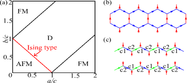
Figure 5: Global phase diagram in plane ($a/c-b/c$) with $V=1$ and snapshots. (a) phase diagram containing AFM, FM and disorder phases (b) the typical snapshot in the FM phase. The AFM-D transition is of Ising type. (c)Two configurations of the AFM phase for the Z2 symmetry breaking.

III.2 Ising type not BKT type of transiton along $a=b$

The phase transitions of the 6V model is identical on both the square lattice and double-layer honeycomb lattice. For example, along $a=b$, Ref. [25] confirms the critical point is at $\beta_{c}=\text{ln}(2)$. The critical point locates at

$$a_{c}=b_{c}=1/2.$$ (19)

In our MC simulation, as shown in Fig. 6 (a)-(b), he intersection of $m_{x}^{-}$ and its Binder ratio $Q$ locates at $a_{c}=b_{c}=1/2$.

However, the type of the phase transition changes. In the $F$ model, the phase transition belongs bo be the BKT type, as evidenced by the non-divergent behavior of specific heats in Fig. 4 in Ref. [25]. In our bilayer 6V model, the type should be Ising type.

The first signature is the value the Ising type critical exponent $\nu=1/y_{t}=1$ satisfys finite size scaling equation defined as follows

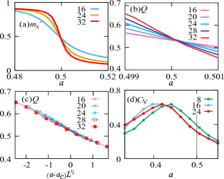
Figure 6: Different quantities scanning $a$ while keeping $a=b$ (a) $m_{x}^{-}$ (b) $Q$ (c) Data collapse of $Q$, while using $y_{t}=1$. (d) Repeating $C_{V}$ of the $F$ model on the square lattice [25].

$$Q= Q_{0}+e_{1}(T-T_{c})L^{y_{t}}+e_{2}(T-T_{c})^{2}L^{2{y_{t}}}$$ (20)

$$+\cdots+f_{1}L^{y_{1}}+f_{2}L^{y_{2}}+\cdots.$$

Using the data clapse method, $Q$ is plotted as function of $(a-a_{c})L^{y_{t}}$, data of different sizes overlap as shown in Fig. 6 (c). This phenomenon supports the conclusion that the observed phase transition is indeed the Ising type.

This type of Ising phase transition can also be analyzed from the perspective of symmetry breaking. In the AFM phase, as depicted in Fig. 5(c), there is a twofold degeneracy in configuration. In the horizontal direction, one configuration is characterized by a c1-c2-c1-c2 vertex arrangement, while the other features a c2-c1-c2-c1 arrangement. Moreover, the relationship between these two configurations is achieved by flipping the states of all legs. This means that from disorder to AFM, there is a Z2 symmetry breaking leading to the Ising transition.

To further confirm our code, we also simulate the F model on the one-layer square lattice, the $C_{V}$ indeed does not diverge at $a_{c}$ as shown in Fig. 6 (d), consistent with the result in Ref. [25].

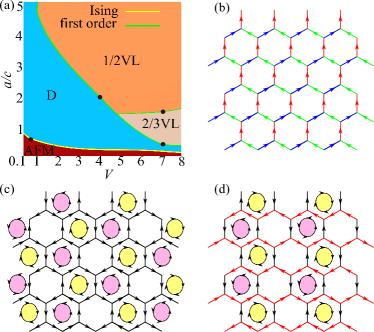
Figure 7: Global phase diagram with $V\neq 1$ and snapshots. (a) A schematic phase diagram (b) the AF phase (c) 2/3 VL phase (d) 1/2 VL phase. In fact, 1/2 VL is accompanied by $x$-direction ferromagnetic order and 1/3 VL is accompanied by AFM order, see appendix A.

IV phase diagram with $V\neq 1$

In this section, we introduce a non-zero value for $v$ in Eq. 1 to discuss the effect the vortex excitation.

As in Ref. [29], it is experimentally possible to manually insert of delete vortices [46, 47], despite the fact that the factors are added manually here.

This phase diagram is shown in the $a-V$ plane, where $V=e^{-v}$, while simultaneously maintaining a fixed cut along the cut $b=a$.

IV.1 global phase diagram

Figure 7 (a) shows the global pahse diagram, which contains the AFM, disorder, 1/2 and 2/3 VL phases. When the vortex excitation is considered, the phase diagram becomes rich. In Fig. 7 (c), the configuration of the 2/3-VL phase is shown. The dual lattice of the honeycomb lattice is the triangular lattice. In this phase, two of the three sets of sublattices within the triangular lattice are occupied by positive and negative vortices, respectively, while the remaining set of sublattices contains no vortices. In Fig. 7 (d), the configuration of the 1/2-VL phase is shown. In this phase, positive and negative vortices alternate sequentially along the $y$-direction, forming connected stripes.

Here, we analyze the distribution of different phases within the phase diagram. When $a$ and $b$ are very small, $a=b\ll c$ and $V\ll c$, the system resides in the AFM phase, represented by the dark red region. The upper right region, $a=b\gg c$ and $V\gg c$, the system corresponds to the 1/2 VL phase. The system has almost no type $c$ vertices. At the same time $V$ drives the system to form vortices consisting of vertices of type $a$, $b$ only, as shown in Fig. A2 (a).

When $a=b\in[0.5c,2c]$, the influence of $V$ drives the system to form vortices consisting of vertices of types $a$, $b$, and $c$, maintaining a 1:1:1 ratio, and the typical configuration of 2/3 VL phase is illustrated in Fig. A2 (b).

In the disordered phase, the characteristics of vortices vary across different parameter regimes. As depicted in Fig. A2 (e), two distinct regimes are identified, labeled as $③$ and $④$.

In the region where $V<1$ and $a(b)$ is large, as shown in Fig. A2 (c), vortices are absent. The reason is that a vortex typically requires the presence of vertices of types $a$, $b$, and $c$, within its structure. Conversely, in the other regime where $V>1$ and reasonable values of $a(b)$ are considered, as illustrated in Fig. A2 (d), numerous vortices appear randomly throughout the system.

In fact, 1/2 VL is accompanied by $x$-direction ferromagnetic order and 1/3 VL is accompanied by AFM order, see appendix A.

IV.2 Vortex structure factors

To further understand the spin vortex lattice phase, the the structure factor in $\bm{q}$-space is introduced as

$$S(\bm{q})=\frac{1}{N_{c}}\sum_{i,j}e^{i\bm{q}\cdot(\bm{r_{i}}-\bm{r_{j}})}\left\langle n_{i}n_{j}\right\rangle,$$ (21)

where $n_{i}$, $n_{j}$ represents 1, 0, in the face of the honeycomb lattices, i.e., triangular lattice. The symbols $\bm{r_{i}}$ and $\bm{r_{j}}$ are the center coordinates of the vortex. In real space, if the density obeys configurations of the form ($101010\cdots$) or ($010101\cdots$), the wave vector corresponding to the maximum value of $S(\bm{q})$ should be located at $\mathbf{q}=(\pi,0)$ [48].

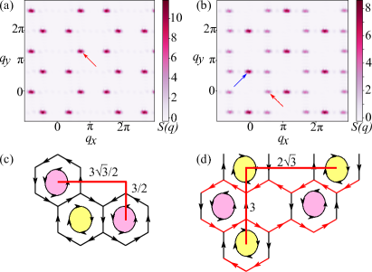
Figure 8: The vortex structure factor $S(\mathbb{q})$ defined in Eq. 21 for (a) 2/3 VL phase (b) 1/2 VL phase in $\mathbb{q}$ space. The translation vectors in real space (c) 2/3 VL phase (d) 1/2 VL phase.

In Fig. 8 (a), for the 2/3 VL phase, $S(q_{x},q_{y})$ is obtained by using Eq. 21 with a lattice size $L=12$. One of the brightest point is located at

$$(q_{x},q_{y})=(\frac{4\sqrt{3}}{9}\pi,\frac{4}{3}\pi),$$ (22)

pointed by the red arrow. The position of the peaks reflects the translational symmetry of the vortex lattice. Assuming that the side length of the honeycomb lattice is 1, the spacing between the two pink vortices $\bm{r_{i}}$ and $\bm{r_{j}}$ is

$$\Delta x=x_{i}-x_{j}=3\sqrt{3}/2,$$ (23)

and

$$\Delta y=y_{i}-y_{j}=3/2.$$ (24)

The positon in Eq. 22 can be obtained by using

$$q_{x(y)}=2\pi/\Delta x(y).$$ (25)

For the 1/2 VL lattice, $S(q_{x},q_{y})$ is shown in Fig. 8 (b). The brightest point (by the blue arrow) is located at

$$(q_{x},q_{y})=(0,\frac{2}{3}\pi),$$ (26)

and the second brightest point (by the red arrow) is located at

$$(q_{x},q_{y})=(\frac{\sqrt{3}}{3}\pi,0).$$ (27)

This is because in real space the translation vectors are respectively $\Delta x=2\sqrt{3}$ and $\Delta y=3$.

In total, we have identified two VL phases in the bilayer 6V model with vortex weight. These ordered states can be distinguished by examining either their respective structure factors or the relevant order parameters.

IV.3 Size effects from periodic boundaries

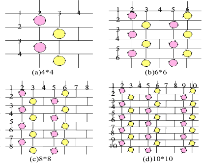
Figure 9: Vortex and anti-vortex in the lattices with $L=4,6,8$ and 10.

Figure 9 shows the size effects of the vortex density in a 2/3 VL with $L=4,6,8,10$, respectively. The honeycomb lattice is a complex lattice with two sites in its smallest cell, hence having an even number of lattice sites in the horizontal direction, i.e., $L\%2==0$.

In Fig. 9(a), for $L=4$, each row contains two faces, one of which is occupied by a vortex. The vortex density, i.e., the ratio between the number of vortices and faces, is $\rho_{v}=N_{v}/N_{f}=1/2$. Similarly, for $L=6,8,10$, the densities become $\rho_{v}=2/3$, 2/4, and 3/5, respectively, as shown in Figs. 9 (b)-(d). In Table 3, we list some possible small sizes and vortex densities.

Table 3: The table shows the maximum theoretical value of the vortex density $\rho_{v}$ as a function of system size $L$

phase	$L$	$4$	$6$	$8$	$10$	$12$	$14$	$16$	$18$	$20$	$L$
2/3 VL	$\rho_{vx}$	$1/2$	$2/3$	$2/4$	$3/5$	$4/6$	$4/7$	$5/8$	$6/9$	$6/10$	$\frac{\lfloor L/3\rfloor}{L/2}$
1/2 VL	$\rho_{vx}$	$1/2$	$1/3$	$2/4$	$2/5$	$3/6$	$3/7$	$4/8$	$4/9$	$5/10$	$~{}\frac{\lfloor L/4\rfloor}{L/2}$

For more general sizes, the densities are as follows:

$$\rho_{v}=\frac{\lfloor L/3\rfloor}{L/2},$$ (28)

where the symbol $\lfloor.\rfloor$ denotes rounding down. We first explain Eq. 28 using $L=6$, two sites labeled as 1, 2 in horizontal direction, totally $L/2$ bricks in each row as shown in denominator.

Then we explain the numerator in Eq. 28. The following three sub-equations explain the number of vortices corresponding to the three sizes $L$, $L+2$, and $L+4$, as shown below: equation

$$\frac{L}{2}\times\frac{2}{3} = \frac{L}{3}\rightarrow\frac{L}{3}=\lfloor\frac{L}{3}\rfloor,$$ (29)

$$\frac{L+2}{2}\times\frac{2}{3} = \frac{L}{3}+\frac{2}{3}\rightarrow\frac{L}{3}=\lfloor\frac{L+2}{3}\rfloor,$$ (30)

$$\frac{L+4}{2}\times\frac{2}{3} = \frac{L}{3}+\frac{4}{3}\rightarrow\frac{L}{3}+1=\lfloor\frac{L+4}{3}\rfloor,$$ (31)

equation where $L+2$ in Eq. (30) indicates two additional sites compared to $L$, i.e., a new empty face without a vortex ($n_{i}=0$), as illustrated by comparing Figs. 9 (b) and (c) in the first lines.

Through the analysis above and the densities presented in Table 3, in the 2/3 VL phase, the density remains constant for sizes where $L\%6==0$. Therefore, when observing physical quantities later, we only simulate systems whose size is a multiple of 6.

IV.4 Detailed transitions between the phases

In this section, our focus is on examining the specific details of phase transitions between multiple phases, and analyzing its underlying reasons.

IV.4.1 The Ising transition between the AFM and disorder phases at $V<1$

Initially, we scan the parameter $a=b\in[0.5,0.8]$ at $V=0.5$, around the black point in the lower left corner of the phase diagram. Various quantities are shown in Fig. 10.

In Figs. 10 (a) and (b), the specific heat $C_{V}$ and $C_{vx}$ exhibit divergence with respect to sizes during the phase transition between the AFM and disorder phases. This behavior stands in contrast to the convergence of $C_{V}$ in the single-layer 6V $F$ model [25], as shown in Fig. 6 (d).

In Figs. 10 (c) and (d), the Binder cumulant $Q$, along with its data collapse at the critical point $a_{c}=0.617$, yields $y_{t}=1$, providing additional confirmation of the Ising transitions.

The possible reasons are as follows: $V<1$ implies the absence of the disordered phase as depicted by the absence of vortices in Fig. A2 (c). Additionally, the AFM phase has no vertex, as illustrated in Fig. 7 (d). Consequently, the phase transition between these two phases does not involve vortices. Moreover, the transition from simple AFM ordering to disorder involves $Z2$ symmetry breaking.

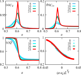
Figure 10: The Ising transition between the AFM and Disorder phases at $V<1$, $a=b$ and $V=0.5$. (a) $C_{V}$ (b) $C_{vx}$, (c) $Q$ (d) data collapse of $Q$, using $y_{t}=1$. The system size ranges from 8 to 24.

IV.4.2 The transitions between the D and 1/2 VL phases at $V>1$

The phase transition between the disorder and 1/2 VL phase is discussed. By fixing the parameter $V=4$, and scanning $a$ and keeping $a=b$, the vortex density $\rho_{vx}$, and $C_{V}$ are measured for different sizes $L=16-48$.

As shown in Fig 11 (a) and (b), the jumps of $\rho_{vx}$ and peaks of $C_{V}$ show the signatures of phase transitions. The divergence of $C_{V}$ confirms the phase transition is not the BKT type [29]. In Figs. 11 (c)-(d), the histogram of $E/N$ and $m_{s}$ are obvious double-peaked at the parameters $a=b=2$. This indicates the phase transition is first-order type.

The signature of the first-order transition can also obtained by fitting the critical exponent. Using the package for finite size scaling [49], $\nu$ is obtained as $0.48(8)$ using Eq. 20.

The data for sizes $L=32,36,40$ overlaps very well. The scaling dimension $y_{t}=1/0.48=2.08\approx 2$ equals to the system dimension $d=2$ when the first-order transition occurs [50].

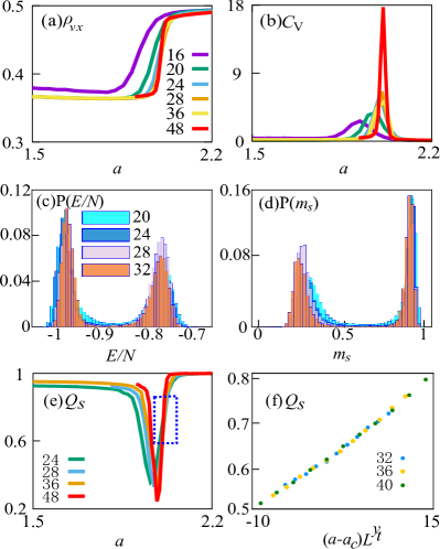
Figure 11: The signatures of the first-order phase transition at $V=4$. The quantities (a) $\rho_{vx}$ (b) $C_{V}$ with system sizes $L=16-48$. The double-peaked distributions (c) $P(E/N)$ and (d) $P(m_{s})$ at $a=2.004(1)$. (e) $Q_{s}$ and (f) data collapse of $Q$ and obtaining $\nu=0.48(8)$ [49].

IV.4.3 The transition between the D and 2/3 VL phases

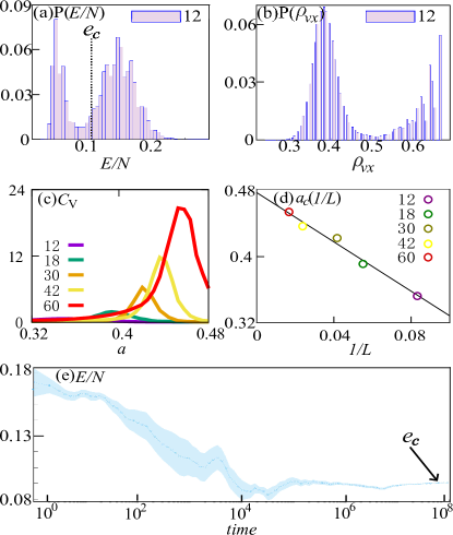
Figure 12: The signatures of the first-order phase transition. The double-peaked distribution of (a) $P(E/N)$ and (b) $P(\rho_{vx})$ at $V=7$ and $a=0.35$. (c) $C_{V}$ versus $a$, (d) $a_{c}$ versus $1/L$. (e) $E/N$ versus MC steps and the convergent time is about $10^{6}$.

The transition from the 2/3 VL phase to the disorder phase is also first order. In Figs. 12(a) and (b), the double peaks in the distribution of $P(E)$ and $P(\rho_{vx})$ indicating a first-order phase transition.

Different from 1/2 VL phase as shown in Fig. 11, this phase transition has an obvious size effect. Figure 12(c) illustrates that the specific heat peak shifts to the right as the size increases. Fortunately, through finite-size scaling defined as follows

$$a_{c}(1/L)=K/L+a_{c}\left(L=\infty\right),$$ (32)

the position of the specific heat converges under the thermodynamic limit $a_{c}\left(L=\infty\right)=0.475811(2)$. The line $a_{c}(1/L)$ versus $1/L$ is shown in Fig. 12(d).

The error bar (2) is calculated by the following equations. First, if one fits $y=kx+b$, then the standard deviation of the intercept b is

$$s_{b}=\sqrt{\frac{n}{n\sum_{i}^{n}x_{i}^{2}-(\sum_{i}^{n}x_{i})^{2}}}\times s_{y}$$ (33)

where $n$ is the number of points involved, $s_{y}$ is the standard deviation of the observation $y_{i}$ and can be expressed as

$$s_{y}=\sqrt{\frac{\sum_{i}^{n}(y_{i}-kx_{i}-b)^{2}}{n-2}}$$ (34)

where $n-2$ is the degree of freedom. If one fits the data using software “gnuplot”, the result is $a_{c}\left(\infty\right)=0.476(5)$ consistent with the above result within the errorbar.

To show that the results are convergent, Fig. 12(e) displays $E/N$ versus MC steps. The converging time is about $10^{6}$ steps. The converged energy is approximately 0.12, denoted as $e_{c}$. $e_{c}$ is also marked by a dashed line in Fig. 12(a), sitting between the two peaks.

IV.4.4 First-order transition between the two vortex lattice phases

Similar to the atomic solid phase in the classical limit [42, 43, 44, 45] for the BH model, the phase transition between 1/2 VL and 2/3 VL phases, should be of the first order. The exact boundary between these two phases can be obtained analytically by comparing the free energy $F=E-TS$ of the both phases.

In tradition, the temperature is set to be $T=1$. By carefully checking, the entropy for the both phase are $S_{1/2}=\ln{64}$ and $S_{2/3}=\ln{36}$, respectively. The entropy does not depend on the lattice size, and therefore, the average entropy for persite denoted as $S/L^{2}/2$ should be zero in the thermal dynamical limit $L\rightarrow\infty$. The energies of the two phases are defined as follows:

$$\left\{\begin{array}[]{lc}E_{1/2\text{VL}}=-L^{2}\ln{a}-L^{2}\ln{b}-\frac{1}{2}L^{2}\ln{V},\\ E_{2/3\text{VL}}=-\frac{2}{3}L^{2}\ln{a}-\frac{2}{3}L^{2}\ln{b}-\frac{2}{3}L^{2}\ln{c}-\frac{2}{3}L^{2}\ln{V}\end{array}\right.$$

where $-L^{2}\ln{a}-L^{2}\ln{b}$ and $-\frac{2}{3}L^{2}\ln{a}-\frac{2}{3}L^{2}\ln{b}-\frac{2}{3}L^{2}\ln{c}$ are the vertex energy for the both phases, and $-\frac{1}{2}L^{2}\ln{V}$ and $-\frac{2}{3}L^{2}\ln{V}$ are the energies for the vortex. Let

$$F_{1/2\text{VL}}=F_{2/3\text{VL}},$$ (35)

with keeping $a=b$, the reduced analytical expression becomes

$$a^{4}=V,$$ (36)

when $L=\infty$.

Numerically simulations also are performed to confirm the first order transition between the vertex phases. In Fig. 13 (a), the distribution of $\rho_{vx}$ for the sizes $L=12,24$ are obtained. In Fig. 13 (b), $\rho_{vx}$ versus $L$ are plotted. The gray data are MC results with 20 independent bins. The theoretical $a_{c}$, are marked by the red line for guide eyes.

In the regime of a strong first-order transition, the cluster algorithm encounters the issue of ergodicity. As a result, we have also incorporated the Metropolis type of short-loop update scheme. In the $z$ direction, the loops connecting two layers can be flipped with a certain probability without violating the “ice” rule for each involved vertex. In order to keep the “two-in two-out” constraint, we flip eight legs as shown in Fig. 13 (c), where the number of 1, 2, 3, 4 mean two of the four legs for each vertex.

In the actual simulation, after each round of loop updates, we will check if there are any short loops present. If a short loop is found, we will attempt to flip it.

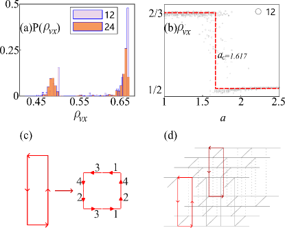
Figure 13: Signal of the first-order phase transition. (a) The double-peaked of the distribution of $\rho_{vx}$, with $V=7$, $a=1.68$ (b) $\rho_{vx}$ versus $a$ (c) a short loop in the vertical direction, and the numbers 1, 2, 3, 4 represent the legs. (d) The Metropolis type of short-loop updating.

V Discussion and conclusion

In this paper, we model two-dimensional two-layer water ice as a two-layer 6V model. By means of the loop update Monte Carlo method, we obtain interesting results.

Our study contrasts the square lattice 6V model, where the AFM to disordered phase transition is governed by the BKT mechanism, with the bilayer 6V model, characterized by a conventional Ising phase transition due to Z2 symmetry breaking. We find that the transitions from vortex lattice phases to the disorder phase and between different vortex lattice phases are both of first order. These insights advance our understanding of the phase transitions present in layered water ices, contributing to the broader comprehension of complex systems in physics.

Despite conducting numerous simulations, there are still many open questions.

(i) As an initial investigation, we have assumed $a=b$, and the case where $a\neq b$ has not been studied yet. The exploration of vortex glass induced by random values of $a$, $b$, and $V$ worthwhile. Furthermore, the disorder we observed can potentially be further classified into disordered structures with vortices and disordered structures without vortices.

(ii) For the bilayer water ice  [21], the systems have various types of boundaries, such as zig-zag and armchair edges, and rough random edges. It is interesting to simulate the bilayer honeycomb 6V model with different boundaries.

(iii) Although we are not clear about how water ice regulates the ratios of $a$, $b$, and $c$ types of vertexes, it is possible to artificially adjust them in the case of artificial spin ice [3], which has many rich physics.

(iv) Regarding the numerical methods for studying this model, not only conventional MC methods are suitable, but tensor network methods [51] are also well-suited for exploring this model. There are existing literature studies that have employed tensor network methods to investigate similar models such as the dimer model and ice model. However, in our case, we introduce a slightly more complex factor by incorporating vortex weighting, which results in an increase in the bond dimensions of the tensor elements.

Acknowledgements We thank Vladimir Korepin and Tzu-Chieh Wei for their inspiration regarding the six-vertex model, and Youjin Deng and Chengxiang Ding for carefully reading and commenting the manuscript. This work was supported by the Hefei National Research Center for Physical Sciences at the Microscale (KF2021002), and Shanxi Province Science Foundation (Grants No: 202303021221029 and No:202103021224051).

Appendix A Configurations with the $a$, $b$, $c$ types vertexes and vortexes

In Figs. A2 (a)-(d), the snapshots of the configurations with vertexes and vortexes are shown. The parameters chosen correspond to the positions marked as ①, ②, ③, ④ in Fig. A2 (e).

In the 2/3 vortex lattice phase, there not only exist vortex orders but also AFM orders with a length of 3 in the $x$-direction Fig. A2 (f). If $y==1$, $S_{y,x}=1$ for $x\in[1,2,3]$ and $S_{y,x}=-1$ for $x\in[1,2,3]$. The definition to quantify such pattern is as follows

$$M_{3}=\sum_{i=1}^{L}\left|\sum_{j=1}^{L}(-1)^{\left\lfloor(j-1)/3\right\rfloor}S_{i,j}\right|/N,$$ (37)

where $\lfloor(j-1)/3\rfloor$ means replacing 1,2,3,4,5 and 6 to 0,0,0,1,1, and 1. Similarily, for the 1/2 VL lattice, there is FM order in the $x$ direction and the quantitiy is defined in Eq. 10.

Appendix B Description of the bounce probabilities

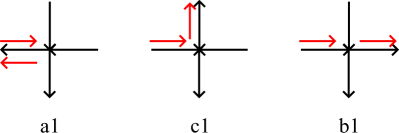
Figure A1: Two allowable exit legs and one bounce leg for the 6V model.

In Sec. II.2, Table 1 shows the range of bounce probabilities $p_{a}$, $p_{b}$ and $p_{c}$. In this appendix, more details are described. Corresponding to the 6V model, the general expression of the bounce probability of the loop algorithm is

$$p_{i}=\frac{w_{i}}{w_{a}+w_{b}+w_{c}},$$ (38)

where the denominator is the sum of the weights of the three vertices after the loop passes through two allowable exit legs and one bounce leg (Fig. A1), and the numerator $w_{i}$ is the weights of the vertices encountered during the loop walk. The subscript $i$ denotes types of $a$, $b$, or $c$. To discuss the range of $p_{i}$, it is only necessary to discuss the maximum and minimum values of Eq. 38, where the variable $w_{c}$ is already fixed to 1. Taking $p_{a}\in(0,1/2)$ in the AFM phase as an example, the weights $w_{a}$ and $w_{b}$ are independently adjustable, but they meet the range $0<a+b<1$, and therefore the maxvalue of $p_{a}=a/(a+b+1)\rightarrow a/(a+1)\rightarrow 1-1/(a+1)=1/2$.

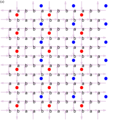
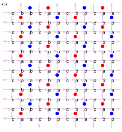
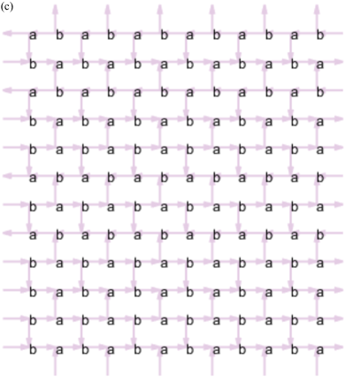
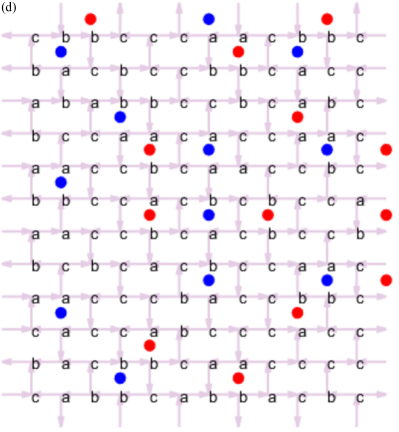
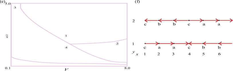
Figure A2: Snapshots for different phases. (a) $\rho_{v}=1/2$ striped vortex lattice (b) $\rho_{v}=2/3$ vortex lattice (c) disorder phase without vortex (d) disorder phase with vortex (e) the four snapshots are obtained at parameters marked in ①, ②, ③ and ④. (f) The AFM pattern with minmum unit length 3 on the 2/3 VL lattice.

References

- Salzmann et al. [2021] C. G. Salzmann, J. S. Loveday, A. Rosu-Finsen, and C. L. Bull, Structure and nature of ice XIX, Nat. Commun. 12, 3162 (2021).
- Bramwell and Gingras [2001] S. T. Bramwell and M. J. P. Gingras, Spin Ice State in Frustrated Magnetic Pyrochlore Materials, Science 294, 1495 (2001).
- Skjrv et al. [2020] S. H. Skjrv, C. H. Marrows, R. L. Stamps, and L. J. Heyderman, Advances in artificial spin ice, Nat. Rev. Phys. 2, 13 (2020).
- Nisoli et al. [2013] C. Nisoli, R. Moessner, and P. Schiffer, Colloquium: Artificial spin ice: Designing and imaging magnetic frustration, Rev. Mod. Phys. 85, 1473 (2013).
- Pauling [1935] L. C. Pauling, The Structure and Entropy of Ice and of Other Crystals with Some Randomness of Atomic Arrangement, J. Am. Chem. Soc. 57, 2680 (1935).
- Harris et al. [1997] M. J. Harris, S. T. Bramwell, D. F. McMorrow, T. Zeiske, and K. W. Godfrey, Geometrical Frustration in the Ferromagnetic Pyrochlore , Phys. Rev. Lett. 79, 2554 (1997).
- Yue et al. [2022] W.-C. Yue, Z. Yuan, Y.-Y. Lyu, S. Dong, J. Zhou, Z.-L. Xiao, L. He, X. Tu, Y. Dong, H. Wang, W. Xu, L. Kang, P. Wu, C. Nisoli, W.-K. Kwok, and Y.-L. Wang, Crystallizing kagome artificial spin ice, Phys. Rev. Lett. 129, 057202 (2022).
- Wang et al. [2006] R. F. Wang, C. Nisoli, R. S. Freitas, J. Li, W. McConville, B. J. Cooley, M. S. Lund, N. Samarth, C. Leighton, V. H. Crespi, and P. Schiffer, Artificial ‘spin ice’ in a geometrically frustrated lattice of nanoscale ferromagnetic islands, Nature 439, 303 (2006).
- King et al. [2021] A. D. King, C. Nisoli, E. D. Dahl, G. Poulin-Lamarre, and A. Lopez-Bezanilla, Qubit spin ice, Science 373, 576 (2021).
- Ramirez et al. [1999] A. Ramirez, A. Hayashi, R. Cava, R. Siddharthan, and B. Shastry, Zero-point entropy in ’spin ice’, Nature 399, 333 (1999).
- Castelnovo et al. [2008] C. Castelnovo, R. Moessner, and S. Sondhi, Magnetic monopoles in spin ice, Nature 451, 42 (2008).
- Latimer et al. [2013] M. L. Latimer, G. R. Berdiyorov, Z. L. Xiao, F. M. Peeters, and W. K. Kwok, Realization of Artificial Ice Systems for Magnetic Vortices in a Superconducting MoGe Thin Film with Patterned Nanostructures, Phys. Rev. Lett. 111, 067001 (2013).
- Ge et al. [2017] J.-Y. Ge, V. N. Gladilin, J. Tempere, V. S. Zharinov, J. Van de Vondel, J. T. Devreese, and V. V. Moshchalkov, Direct visualization of vortex ice in a nanostructured superconductor, Phys. Rev. B 96, 134515 (2017).
- Vlasko-Vlasov et al. [2014] V. K. Vlasko-Vlasov, J. R. Clem, A. E. Koshelev, U. Welp, and W. K. Kwok, Stripe Domains and First-Order Phase Transition in the Vortex Matter of Anisotropic High-Temperature Superconductors, Phys. Rev. Lett. 112, 157001 (2014).
- Maiorov et al. [2000] B. Maiorov, G. Nieva, and E. Osquiguil, First-order phase transition of the vortex lattice in twinned single crystals in tilted magnetic fields, Phys. Rev. B 61, 12427 (2000).
- Zeldov et al. [1995] E. Zeldov, D. Majer, M. Konczykowski, V. B. Geshkenbein, V. M. Vinokur, and H. Shtrikman, Thermodynamic observation of first-order vortex-lattice melting transition in Bi2Sr2CaCu2O8, Nature 375, 373 (1995).
- Sasagawa et al. [1998] T. Sasagawa, K. Kishio, Y. Togawa, J. Shimoyama, and K. Kitazawa, First-order vortex-lattice phase transition in (La1-xSrx)2CuO4 single crystals: Universal scaling of the transition lines in high-temperature superconductors, Phys. Rev. Lett. 80, 4297 (1998).
- Kosterlitz and Thouless [1972] J. M. Kosterlitz and D. J. Thouless, Long range order and metastability in two dimensional solids and superfluids. (Application of dislocation theory), J. Phys. C: Solid State Phys. 5, L124 (1972).
- Kosterlitz [2017] J. M. Kosterlitz, Nobel Lecture: Topological defects and phase transitions, Rev. Mod. Phys. 89, 040501 (2017).
- Berezinsky [1970] V. Berezinsky, Destruction of long range order in one-dimensional and two-dimensional systems having a continuous symmetry group. I. Classical systems, J. Exp. Theor. Phys. 32, 493 (1970).
- Ma et al. [2020] R. Ma, D. Cao, C. Zhu, Y. Tian, J. Peng, J. Guo, J. Chen, X.-Z. Li, J. S. Francisco, X. C. Zeng, L.-M. Xu, E.-G. Wang, and Y. Jiang, Atomic imaging of the edge structure and growth of a two-dimensional hexagonal ice, Nature 577, 60 (2020).
- Koga et al. [1997] K. Koga, X. C. Zeng, and H. Tanaka, Freezing of Confined Water: A Bilayer Ice Phase in Hydrophobic Nanopores, Phys. Rev. Lett. 79, 5262 (1997).
- Zhu et al. [2018] W. Zhu, Y. Zhu, L. Wang, Q. Zhu, W.-H. Zhao, C. Zhu, J. Bai, J. Yang, L.-F. Yuan, H. Wu, and X. C. Zeng, Water Confined in Nanocapillaries: Two-Dimensional Bilayer Squarelike Ice and Associated Solid–Liquid–Solid Transition, J. Phys. Chem. C 122, 6704 (2018).
- Syljuåsen and Zvonarev [2004a] O. F. Syljuåsen and M. B. Zvonarev, Directed-loop Monte Carlo simulations of vertex models, Phys. Rev. E 70, 016118 (2004a).
- Weigel and Janke [2005] M. Weigel and W. Janke, The square-lattice F model revisited: a loop-cluster update scaling study, J. Phys. A: Math. Gen. 38, 7067 (2005).
- Ising [1925] E. Ising, Beitrag zur Theorie des Ferromagnetismus, Z Med Phys 31, 253 (1925).
- Wu [1982] F. Y. Wu, The Potts model, Rev. Mod. Phys. 54, 235 (1982).
- Ma et al. [2024] H. Ma, W. Zhang, Y. Tian, C. Ding, and Y. Deng, Emergent topological ordered phase for the Ising-XY Model revealed by cluster-updating Monte-Carlo method, Chin. Phys. B (2024).
- Zhao et al. [2018] R. Zhao, C. Ding, and Y. Deng, Overlap of two topological phases in the antiferromagnetic Potts model, Phys. Rev. E 97, 052131 (2018).
- Belov and Reshetikhin [2022] P. Belov and N. Reshetikhin, The two-point correlation function in the six-vertex model, J. Phys. A: Math. Theor. 55, 155001 (2022).
- Lyberg et al. [2017] I. Lyberg, V. Korepin, and J. Viti, The density profile of the six vertex model with domain wall boundary conditions, J. Stat. Mech. : Theory Exp. 2017, 053103 (2017).
- Kubo et al. [1988] K. Kubo, T. A. Kaplan, and J. R. Borysowicz, Monte Carlo simulation of the S=1/2 antiferromagnetic Heisenberg chain and the long-distance behavior of the spin-correlation function, Phys. Rev. B 38, 11550 (1988).
- Sandvik [2003] A. W. Sandvik, The Directed-Loop Algorithm, in AIP Conf. Proc. (AIP, 2003).
- Syljuåsen and Zvonarev [2004b] O. F. Syljuåsen and M. B. Zvonarev, Directed-loop Monte Carlo simulations of vertex models, Phys. Rev. E 70, 016118 (2004b).
- Prokof’ev et al. [1998] N. Prokof’ev, B. Svistunov, and I. Tupitsyn, “Worm” algorithm in quantum Monte Carlo simulations, Physics Letters A 238, 253 (1998).
- Prokof’ev and Svistunov [2001] N. Prokof’ev and B. Svistunov, Worm Algorithms for Classical Statistical Models, Phys. Rev. Lett. 87, 160601 (2001).
- Deng et al. [2007] Y. Deng, T. M. Garoni, and A. D. Sokal, Dynamic Critical Behavior of the Worm Algorithm for the Ising Model, Phys. Rev. Lett. 99, 110601 (2007).
- Wang et al. [2021a] B.-Z. Wang, P. Hou, C.-J. Huang, and Y. Deng, Percolation of the two-dimensional model in the flow representation, Phys. Rev. E 103, 062131 (2021a).
- Chen et al. [2022] H. Chen, P. Hou, S. Fang, and Y. Deng, Monte Carlo study of duality and the Berezinskii-Kosterlitz-Thouless phase transitions of the two-dimensional -state clock model in flow representations, Phys. Rev. E 106, 024106 (2022).
- Zhang et al. [2020] L. Zhang, M. Michel, E. M. Elçi, and Y. Deng, Loop-Cluster Coupling and Algorithm for Classical Statistical Models, Phys. Rev. Lett. 125, 200603 (2020).
- Kao and Melko [2008] Y.-J. Kao and R. G. Melko, Short-loop algorithm for quantum Monte Carlo simulations, Phys. Rev. E 77, 036708 (2008).
- Zhang et al. [2010] W. Zhang, L. Li, and W. Guo, Hard core bosons on the dual of the bowtie lattice, Phys. Rev. B 82, 134536 (2010).
- Zhang et al. [2015] W. Zhang, Y. Yang, L. Guo, C. Ding, and T. C. Scott, Trimer superfluid and supersolid on two-dimensional optical lattices, Phys. Rev. A 91, 033613 (2015).
- Zhang et al. [2014] W. Zhang, R. Li, W. X. Zhang, C. B. Duan, and T. C. Scott, Trimer superfluid induced by photoassocation on the state-dependent optical lattice, Phys. Rev. A 90, 033622 (2014).
- Zhang et al. [2013] W. Zhang, R. Yin, and Y. Wang, Pair supersolid with atom-pair hopping on the state-dependent triangular lattice, Phys. Rev. B 88, 174515 (2013).
- Chen et al. [2016] T.-W. Chen, S.-D. Jheng, W.-F. Hsieh, and S.-C. Cheng, Vortex and trapped states of microcavity-polariton condensates in a harmonic trap, Comput. Mater. Sci. 117, 579 (2016).
- Xu et al. [2006] K.-X. Xu, J.-H. Qiu, and L. yi Shi, Non-power-law I–V characteristics in Ca-doped polycrystalline Y1-xCaxBa2Cu3O7-δ, Supercond. Sci. Technol. 19, 178 (2006).
- Wei et al. [2021] H. Wei, J. Zhang, S. Greschner, T. C. Scott, and W. Zhang, Quantum Monte Carlo study of superradiant supersolid of light in the extended Jaynes-Cummings-Hubbard model, Phys. Rev. B 103, 184501 (2021).
- Melchert [2009] O. Melchert, autoScale.py - A program for automatic finite-size scaling analyses: A user’s guide (2009), arXiv:0910.5403 [physics.comp-ph] .
- Wang et al. [2021b] Z. Wang, L. Feng, W. Zhang, and C. Ding, Phase transitions in a three-dimensional Ising model with cluster weight studied by Monte Carlo simulations, Phys. Rev. E 104, 044132 (2021b).
- Xie et al. [2009] Z. Y. Xie, H. C. Jiang, Q. N. Chen, Z. Y. Weng, and T. Xiang, Second renormalization of tensor-network states, Phys. Rev. Lett. 103, 160601 (2009).