Polynomial-time derivation
of optimal -tree topology from Markov networks
Abstract
Characterization of joint probability distribution for large networks of random variables remains a challenging task in data science. Probabilistic graph approximation with simple topologies has practically been resorted to; typically the tree topology makes joint probability computation much simpler and can be effective for statistical inference on insufficient data. However, to characterize network components where multiple variables cooperate closely to influence others, model topologies beyond a tree are needed, which unfortunately are infeasible to acquire. In particular, our previous work has related optimal approximation of Markov networks of treewidth closely to the graph-theoretic problem of finding maximum spanning -tree (MST), which is a provably intractable task.
This paper investigates optimal approximation of Markov networks with -tree topology that retains some designated underlying subgraph. Such a subgraph may encode certain background information that arises in scientific applications, for example, about a known significant pathway in gene networks or the indispensable backbone connectivity in the residue interaction graphs for a biomolecule 3D structure. In particular, it is proved that the -retaining MST problem, for a number of classes of graphs, admit -time algorithms for fixed . These -retaining MST algorithms offer efficient solutions for approximation of Markov networks with -tree topology in the situation where certain persistent information needs to be retained.
Keywords: Markov network, joint probability, KL divergence, mutual information, -tree, tree-width, -retaining spanning graph, dynamic programming
1 Introduction
To accurately model complex real world systems that exhibit relationships among random variables, it is often crucial to compute the joint probability distribution of a set of random variables [1, 2]. The joint distribution function , for set of random variables, serves as a fundamental basis for a wide range of statistical and probabilistic modeling techniques employed in many fields, such as communication, pattern recognition, machine learning, information retrieval, databases, and learning systems [3, 4, 5]. Distribution captures the relationships and dependencies between different variables or events within the system. It provides insights into the likelihood of specific outcomes, helps identify patterns and correlations, and enables prediction of unseen data [6, 7]. It can be challenging, and sometimes even impossible within a reasonable time frame, to determine a single probability distribution due to the complex relationships between random variables. For example, to fully specify the -order probability distribution of an event space defined by binary random variables, the knowledge of probability values would be required. Indeed, the exponential size of the event space makes the exact learning of to be an intractable task [8, 7, 9]. The challenge becomes even greater when only limited number of data samples are at hand [10].
Various approaches to approximate have proposed for situations where the information of random variables is given with a limited number of samples [11, 10, 12, 6, 13, 14, 7, 15]. One common approach is to approximate the -order using a lower-order probability function. Lower-order approximations encompass the -order approximations for . These approximations often involve simplifying assumptions, such as statistical independence or other constraints imposed on dependency relationships between the random variables. By employing these techniques, it becomes possible to compute a specific joint probability distribution that aligns with the available data. Their effectiveness is contingent upon the accuracy of approximations in capturing the true distribution . In a study by King et al. [16], the authors specifically focused on a second-order approximation () to approximate a multivariate probabilistic model. The second-order approximation considers only the pairwise dependency between variables, reducing the computational complexity of calculating to .
The seminal work of Chow and Liu [10] has made a significant contribution to the field of approximating using a second-order approximation method with a tree-topology known as the Chow-Liu tree. Technically, this approximation method constructs a maximum spanning tree of the network whose topology guarantees to minimize information loss in approximating , as measured by the Kullback-Leibler divergence [17]. The Chow-Liu method has been proven both practical and computationally efficient, even with limited data availability [18, 15]. In various applications, in the context of either physical or artificial systems, such a tree structure often serves as an effective model for approximating the underlying system[19]. As a result, the Chow-Liu tree is widely employed as a flexible and interpretable model across different tasks, including dimensional reduction [20] systems biology [21], gene differential analysis [12], discrete speech recognition [14], data classification and clustering tasks [22], and time-series data analyses [23].
However, an approximation of probability distribution with tree topology may be below the desired or expected level of performance when dealing with distributions of high-dimensional data. In many real world scenarios, dependencies and relationships between variables are often more complex than what a tree structure can capture [24, 15, 25]. Specifically, the tree topology fails to deal with the scenario where one variable is an effect caused by collaborative work of two or more other variables [26]. Even in real world applications that exhibit tree-like (sparse) network structures, [27], there exist critical components that may not be a tree structure. One such example is a bottleneck component of several genes working together to influence a couple of downstream genes in a cancerous pathway within a gene-network [28]. Networks containing such locally coupled components while demonstrating global sparsity are common, e.g., a social network containing small groups of highly related people, an article citation network for advancement of specific research topic, and a biological network including a cluster of interacting proteins [29, 30].
Hence, approximation of probability distribution with sparse, non-tree graph topology is desirable; yet measuring the quality of approximation requires an accurate definition of network sparsity. Sparsity of a graph is often loosely defined by the ratio of the number of edges to the number of vertices in the graph. Typically a graph is sparse if , i.e., the number of edges is at most linearly related to the number of vertices. This metric, while intuitive, may not account differences in global topology among such graphs. For example, “tree-like” graphs bear very different global connectivity from those “grid-like” graphs, in spite of both having a linear number of edges. The global connectivity of graphs can have an immediate impact on the tractability of graph optimization problems, which can be well quantified with the notion of graph “tree width”. Tree-width measures how much a graph is tree-like and it is intimately related to the notion of -tree [31, 32, 33]. Indeed, under various settings, investigations have been carried out on approximation of with topology of graphs of small tree-width [25, 34, 35]. In particular, our previous work connects the optimal approximation of with graph topology of tree-width to the task of finding a maximum spanning -tree (MST) from the underlying network graph [36]. The latter task, unfortunately, is computationally intractable [37] for all fixed .
In this paper, we investigate efficient algorithms for optimal Markov network approximation with graph topology of tree-width bounded by under natural condition arising from applications, specifically when the desired topology of tree-width retains certain essential subnet in the underlying Markov network. We coin this the problem -retaining MST, which finds a maximum spanning -tree that retains a subgraph (of class ) designated in the input graph. We prove that for class of bounded degree spanning trees, the -retaining MST problem can be solved in polynomial-time on graphs of vertices for every fixed . We also show that the achieved time complexity upper is likely the optimal for problem -retaining MST. In particular, we are able to reduce the classical graph problem -Clique to -retaining MST with a transformation that literally preserves the parameter value. Problem -Clique is notoriously difficult to admit algorithms of time , for [38, 39] or for constant and function of only [40]. Our presented transformation passes these difficulties of -Clique onto problem -retaining MST.
The algorithms for -retaining MST solving optimal Markov network approximation are also practically useful for solving other scientific problems. In particular, since Hamiltonian paths constitutes a special class of bounded-degree spanning trees, the algorithms can be tailored to solving problem Hamiltonian path-retaining MST. This is especially useful for revealing hidden higher-order relationships over a set of random variables that possess an indispensable total order relation, e.g., time series data, linguistic sentences, and biomolecule sequences. Indeed, our work has inspired a general framework for efficient and accurate prediction of biomolecule 3D structures. According to this framework, on a given molecule consisting of an ordered sequence of residues, an underlying probabilistic graph can be formulated in which random variables represent residues, edges for possible interactions between residues, and “backbone edges” connecting neighboring residues on the sequence. The objective of the 3D structure prediction problem is to find a spanning -tree, which maximizes sum of mutual information of all involved -cliques in the -tree. Here the mutual information of four variables in a -clique is defined based on its probabilistic mapping to a tetrahedron motif involving 4 residues in the biomolecule, where tetrahedrons are geometric building blocks of the 3D structure [36].
2 Preliminaries
In this section, we introduce the notions of Markov networks, -tree, tree-width, and Markov -tree, which play essential roles in discussions throughout the paper.
2.1 Markov Networks
A finite system comprising random variables is denoted as , with the joint probability distribution function . While may offer insights into dependence relationships among the variables, it is often not known due potentially high-dimensional relationships among the variables. The task we are interested in is to approximate the joint probability distribution with , a joint distribution of in their binary relationships characterized by graph . We call the topology of .
Definition 1
Let be a non-directed probabilistic graph with vertex set consisting of random variables and edge set . is called a Markov network if, for the joint probability distribution ,
| (1) |
That is, variables and without sharing an edge are conditionally independent given the the rest of variables in the graph.
2.2 -tree and tree-width
Tree-width is a metric on graphs that measures how much a graph is tree-like. There are a few alternative definitions for tree-width. The one most relevant to this work is via the notion of -tree.
Definition 2
Let be an integer. The class of graphs called -trees are defined recursively based on the number of vertices they contain:
-
1.
A -tree of exactly vertices is a -clique;
-
2.
A -tree of vertices, for any , consists of a -tree of vertices and a vertex , such that, for some -clique in ,
(a) ;
(b) .
When , -trees are 1-trees, which are simply trees under the regular sense [33]. However, for , -trees are not trees as they contain cycles. We call any subgraph of a -tree a partial -tree.
Definition 3
Let be a graph. Then the tree-width of is the smallest number for which is a partial -tree.
Apparently any -tree is a graph of tree-width . The following assertion gives a stronger relationship between graphs of tree-width and -trees.
Proposition 1
For every fixed , -trees are maximum graphs of tree-width .
As defined, a -tree with vertices is generated through a recursive process that constructs a sequence of (sub)--trees whose numbers of vertices are . During the generations, vertices and edges are created via rules 1 and 2 in Definition 2. This leads to the following further notes on the notion of -tree.
First, by Definition 2, every vertex in a -tree is generated with respect to a certain subset of other vertices. Typically, an application of rule 2 generates a new vertex and associates it with an existing clique of vertices to form a -clique. For vertices in the -clique generated by rule 1, no explicit association of a vertex to others is given. If vertices in the -clique are considered generated one at a time, like by rule 2, then there is an assumed precedence order in the -clique such that vertex precedes vertex if and only if is generated with respect to .
Definition 4
Let be a -tree for some . A associated precursor function for is a mapping that designates a subset of vertices for every vertex , such that
(1) if is generated with rule 2 of Definition 2, then , where is given by rule 2, or
(2) if , the -clique created with rule 1, then ; and ,
if and only if .
Note that case (2) of precursor function imposes a total order for the vertices in set generated by rule 1 and hence there exists a vertex, named , such that . Specifically, vertices in set are ordered as if and only if where , .
Second, different construction processes of the same -tree may result in different associated precursor function. In this paper, when a -tree is assumed, some associated precursor function is also assumed.
Third, based on Definition 2, the total number of -cliques in the -tree of vertices, for , is exactly .
2.3 Markov -tree:
Definition 5
Let be an integer. A Markov -tree is a Markov network over random variables with a topology graph being a -tree. The joint probability distribution function of the Markov -tree is defined by :
| (3) |
where is some associated precursor function222 Our previous [36] work proves that the joint probability defined for a given Markov -tree is invariant of its associated precursor function .. Note that the joint probability given in equation 3 has the right-hand-side that is actually derived using the chain-rule of multivariate probability and conditional independence by Markov properties. Specifically, the right-hand-side is obtained by following the reversed process of constructing the -tree that corresponds to the associated precursor function .
2.4 Mutual information
Our discussions on approximation of Markov networks are based on Shannon’s information theory.
Definition 6
Let be a finite set of random variables with distribution . Then the entropy of variables is defined as .
While the Shannon’s entropy accounts for the averaged number of (binary) bits to encode random variable values of one distribution, another notion of entropy can be used to measure the difference between two distributions [17].
Definition 7
Let and be two distributions for the set of random variables. Then the relative entropy or Kullback–Leibler divergence between and is defined as
| (4) |
In particular, with representing the joint probability between two random variables and and representing their independence distribution, we obtain
Definition 8
Let be a joint distribution for random variables and . Their mutual information is defined as
| (5) |
Equation 5 can be extended to the following mutual information between a single variable and a set of random variables:
| (6) |
3 Approximation with -tree topology
We now discuss approximate of Markov networks with topologies specified with graphs. Let be a set of random variables and be a probabilistic distribution of a Markov network over variables with an unknown topology. For graph , with , we denote with the distribution of a Markov network over random variables with topology .
Definition 9
Let integer and be a class of graphs (of vertices). The optimal approximation of with topology is a distribution such that
Chow and Liu [10] initiated a seminal work on approximation with the topology class of trees. They proved that for the tree class, the optimal approximation is via a tree topology that yields the maximum sum of mutual information , where is the predecessor variable of variable . Such a tree can be found by the algorithm that solves the maximum spanning tree problem in linear time.
Our previous work [36] extended the result to the topology class of -trees and show that the optimal approximation can be achieved with a spanning -tree topology yielding the maximum mutual information
| (7) |
for any associated precursor function .
The derivation of the result in (7) is based on the connection between the minimization of the KL-divergence and the maximization of a spanning -tree, as follows. Let be a spanning -tree with an associated precursor function . Applying equation 3 to the KL-divergence formula
| (8) |
to yield
| (9) |
where the is over all values of and the last term on the right-hand-side of the last equation in (9) can be rewritten as
| (10) |
where the second last equality holds because is projected on component and component with values over other components summed up to 1.
Because both in (9) and in (10) are invariant of the choice of topology , combining equations (10) with (9) leads to the conclusion that a topology to minimize distance if and only if it maximizes sum of mutual information , where is any associated precursor function with .
We now turn the latter problem into a graph-theoretic problem. Let be an integer and be the positive integer set.
Definition 10
Let be a function. The problem -based maximum spanning -tree, denoted with MST, is defined as: given an underlying non-directed graph , finds a maximum spanning -tree of such that the objective function achieves the maximum, where is a -clique in .
Note that to make the problem MST well defined, the input graph needs to include values of function over some (but not necessarily all) -cliques in the graph. We often omit from the problem name MST, leaving it just MST, when is known in the context or without being specifically referred to in a discussion.
Theorem 1
The optimal approximation of Markov networks with -tree topology can be achieved by solving the problem MST, where for every -clique , .
Unfortunately, the intractability of the following problem makes MST difficult to solve.
Proposition 2 ([37])
The following decision problem is NP-hard on every fixed : Determining if a given graph possesses a spanning -tree as its subgraph.
4 -retaining MST
We now turn into a restricted version of problem MST.
Definition 11
Let be a class of graphs. -retaining MST is the MST problem whose outputted maximum spanning -tree is required to include some spanning subgraph designated in the input graph .
By the definition, in the graph as the input for the -retaining MST problem, a spanning subgraph of , which belongs to the class , needs to be specified. Our discussion will be focused on that is specifically the class of bounded-degree spanning trees. That is, problem -retaining MST requires its outputted maximum spanning -tree to retain the designated bounded-degree spanning tree from the input graph .
Lemma 1
Let be a -tree with vertices. Then
(1) Every edge in belongs to some -clique in .
(2) During creation of with Definition 2, no edge can be created after and have
been created. That is, edge can only be created when either or being created.
Definition 12
Let be a -tree, , and be any -clique in . Then any -clique in is called a neighbor of if .
Definition 13
Let a subset of vertices in graph . separates the graph into two or more disconnected components if disjoins with all these components and any path connecting vertices between any pair of the disconnected components should contains some vertex in .
Lemma 2
Let be a -tree and be a -clique in . Assume that separates into connected components. Then the number of neighbors for is at most .
Proof:
Let be a -clique in the -tree . Denote with the set of all neighbors of .
Let be two neighbors of and are two vertices such that and . It is clear that and . We claim that and cannot belong to the same connected component due to the separation of by the -clique .
To see the claim is true, consider otherwise there is a path , for some , connecting and , where , and the set of vertices on is completely disjoint with . By Lemma 1, it is obvious that for any edge in , the edge has to be created along with either of its end vertices. This means either edge or is the last edge on to be created.
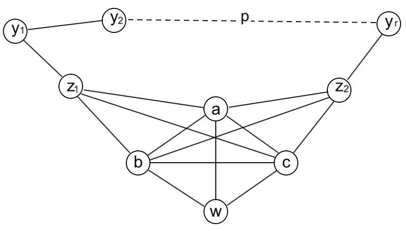
Without loss of generality, assume is the last edge on to be created. It implies that and have been created earlier. Then there are only two scenarios to consider. (1) -clique was created along with being created. This implies that -clique had already existed and that consequently either -clique or edge cannot be created. See Figure 1. Contradicts. (2) was created before -clique is created. Based on the argument for case (1), -clique can only be created after -clique , which also suggests that cannot be created since has already existed. Contradicts.
The above argument shows that for any two vertices and , where are neighbors of -clique , and belong to two different connected components separated by . So if the number of connected components is , .
Definition 14
A -tree has bounded branches if every -clique in has a bounded number of neighbors. A graph is bounded branching-friendly if every -tree that contains as a spanning subgraph has bounded branches.
Theorem 2
Let be the class of bounded-degree trees. Then any graph in is bounded branching friendly.
Proof: Let be any bounded-degree tree in . We will show that every -tree that contains as a spanning tree has bounded branches. That is to show that every -clique in -tree separates into a bounded number of connected components, and then by Lemma 2, every -clique in such a has bounded number of neighbors.
Assume constant to be the highest degree of vertices in and let be any -clique in the -tree that contains as a spanning tree. Let be any subset of vertices, with . We claim that the number of connected components in separated by is at most . We prove the claim by induction on .
When , contains only one vertex, which can separate into at most components. Since is a spanning tree of , the vertex can separate into at most components
Assume contains vertices and it separates into at most connected components. Consider now the case that contains vertices. Let vertex . By assumption, set should separates into at most connected components. Let be one such component that belongs to. Then can further separate subgraph , thus subgraph into at most components. Together with the other components, these are connected components separated by of vertices.
Apply the proved claim to -clique , it is clear that separates into at most connected components. Since is an arbitrary -clique in , by Lemma 2 and Definition 14, has bounded branches. And again by Definition 14, we conclude that in is bounded branching friendly.
Corollary 1
Let be the class of Hamiltonian paths. Then any graph in is bounded branching friendly.
5 Algorithm
In this section, we show that, for any bounded branching friendly class of graphs, the -retaining MST problem can be solved in polynomial time for every fixed . We will discuss such an algorithm extensively for that is the class of bounded-degree spanning trees, which can be generalized to any bounded branching friendly class .
5.1 Tree-decomposition representation
We first introduce some further notations to facilitate discussions. Consider again Definition 2 for -trees. It is clear that every -tree consists of a collection of -cliques. Every -clique is created as , exclusively along with a newly introduced vertex . On the other hand, there may be more than one -clique that contains the whole set of vertices. To establish succinct relationships between -cliques, recursively we label every -clique uniquely as , where is the newly introduced vertex for creation of the -clique and satisfies:
(1) either , or
(2) -clique , for some and , which is created earlier, with
.
In (2), is called the parent of , denoted with . It is clear that every -clique, except the one first created (that does not have a parent), has a unique parent.
Proposition 3
The relation defined by parent between -cliques in -tree forms a rooted-tree topology , where
(1) ;
(2) , for some , is the designated root;
(3)
We call a tree-decomposition333The notion of tree-decomposition was first introduced independently from the notion of -tree [32]. It is used in this section solely for the purpose of discussion our algorithms on -trees. of -tree . We have the following important property for tree-decomposition.
Proposition 4
Let and be two -cliques on a tree-decomposition of -tree . Let vertex . Then for every -clique on the path between and on the tree.
Proof: Since is on the path between and on the tree, there are only two scenarios about their creations. (1) is an “ancestor” of both and . (2) is a descendent of one and an ancestor of another. In both scenarios, if , there are duplicated creations of vertex , contradicting that -tree definition.
The notation of tree-decomposition offers a higher level view on a -tree and makes the discussion easier on algorithms for -tree optimization. In particular, construction of a -tree is equivalent to construction of the tree-decomposition of the corresponding -tree.
Specifically, the tree-decomposition of a -tree is a tree rooted at -clique for some , with tree nodes, both internal and leaf nodes, drawn from set . Since the tree is rooted, it is directional. Therefore, -clique is an internal node with a child node , for any , if and only if . Formally, we need the following technical results in the next section.
Definition 15
Let be a tree-decomposition of -tree , with root , . For any , we define subset of , such that
Clearly, if is the root node of any tree decomposition, then .
Proposition 5
Let be a tree-decomposition of -tree . Then the subtree rooted at -clique is a tree-decomposition of the induced subgraph of the -tree by vertex set .
5.2 Dynamic programming
By Proposition 5, a tree-decomposition for -tree can be constructed by building sub-tree-decompositions and assemble them into the whole tree-decomposition. This leads to the following repetitive (thus recursive) process to construct a tree-decomposition . Specifically, let be an internal node of the tree with children , , for some . Building the subtree rooted at with the children can be done by first connecting child to and then continuing to build the subtree rooted at with the rest of the children , .
We now discuss the details. To create the child from parent node , vertex in can only be one that was not created before. This means that the creation process needs to keep the record of an exact set from which a new vertex can be drawn for creation of a subtree rooted at . Because is a class of bounded branches friendly graphs, by the proofs of Lemma 2 and of Proposition 4, this set of vertices is actually partitioned into at most exclusive subsets, for some constant ; vertices from only one of these subsets can be drawn for creation of the subtree. In other words, these subsets correspond to some of the connected components of separated by the -clique . Since is a known subgraph given in the input graph , vertices in every one of these subsets are known when is specified. This suggests that every subset can be retrieved with an index identifier and there are a constant number of such indexes for these exclusive subsets.
Specifically, assume to be the largest number such that is separated by any -clique into at most connected components. Let denote the set . Given tree node (i.e., -clique) , let denote the function that maps any identifier to the set of vertices in the connected component (resulted from the separation by ). Then the set of vertices in the subtree rooted at , excluding those in , can be written as , for some subset . We will show that that set is uniquely determined by along with during the tree construction process.
Definition 16
Let be a real-value function with the argument being a -clique. We define real-value function to be the maximum sum of values over all -cliques (excluding ) in a subtree rooted at that contains vertices in .
Then we can derive the following recurrence for function :
| (11) |
where is a subset of identifiers for the connected components of separated by .
The recurrence (11) has the base cases , for all .
Lemma 3
Recurrence (11) together with its base cases computes correctly function .
Proof: We prove the claim by showing that the recurrence computes correctly the sum of scores on all -cliques in the subtree rooted at , excluding itself. We do this by induction on , the number of -cliques in the subtree rooted at .
When , the subtree contains only -clique itself. This corresponds to the case case which has value 0.
We hypothesize that when , the claim is correct. Consider the case . Note that node , the root of the subtree, has children nodes, each of which is the root of the subtree containing exactly the vertices in one of the connected components separated by . The recurrence first adds term into the sum, where is one of the children node and the root of the subtree covering the connected component. Term recursively computes the sum of scores on the rest of -cliques in the subtree covering the connected component. Term recursively computes the sum of scores on the rest of subtrees rooted at . In both cases, the numbers of -cliques to compute are at most and they are both correct by the hypothesis.
Now we justify that given -clique and identifiers , the information of vertices belonging to connected components (of separated by ) can be determined. Consider vertices in are identified on , upon which a search process (e.g., depth-first search) on can determine connected components. Vertices are associated with these components and each component is associated with an identifier in . The component that vertex belongs, which can be determined, should be in set . The same argument applies to .
Since Recurrence (11) maximizes the sum of scores on all -cliques of the subtree rooted at a -clique except the root, the answer to the -retaining MST problem can be expressed as:
| (12) |
by examining all possible roots for a maximum spanning -tree.
Function can be implemented with a dynamic programming algorithm based on the recurrence equation (11). This essentially involves establishing a look-up table that computes values of function on all necessary combinations of . For graph of vertices, the table size is and each entry in the table can be computed in time for selecting vertex . This gives rise to the time complexity .
Theorem 3
Let be the class of all bounded branches friendly graphs. The -retaining MST problem can be solved in time , for every fixed .
Theorem 4
Given any Markov network of random variables, its -tree topology approximation with the minimum loss of information can be computed in time , for every fixed , provided that the found topology retains some designated spanning graph that is bounded branches friendly.
Corollary 2
There are polynomial time algorithms for the minimum loss of information approximation of Markov networks with a -tree topology that retains a designated Hamiltonian path in the input network.
Corollary 3
There are polynomial time algorithms for the minimum loss of information approximation of Markov networks with a -tree topology that retains a designated bounded-degree spanning tree in the input network.
5.3 Optimality in complexity
An early study [42] on the -retaining MST problem showed that, for the class of Hamiltonian paths, the algorithm can be tweaked such that the time complexity can be improved to . We believe the technique and the time bound can be generalized to all bounded branches friendly classes . We omit such a proof which is rather lengthy.
However, the polynomial time for -retaining MST may not be further improved in term of its exponent parameter . In the following we show strong evidence that this claim is true. For this we defined the following decision problem related to -retaining MST with being the class of Hamiltonian paths. We assume is real-value function with argument being a -clique together with weights of edges they share.
H-MST:
Input: edge-weighted graph with an Hamiltonian path , integer , real number ;
Output: “Yes” if and only if there is a spanning -tree retaining whose sum of scores
over all -cliques is at least ;
We now connect problem H-MST to the classical graph-theoretic problem -Clique, which determines if the input graph has a clique of size as the given threshold . While -Clique problem can be solved trivially in time on graph of vertices, any substantial improvement to the upper bound has proved extremely difficult. In particular, it is unlikely [38, 39] to solve problem -Clique in time for any . In addition, it has also been proved [40] that solving -Clique in time , for some function independent of and some constant would lead to an unlikely breakthrough in computational complexity theory. We will show such difficulties for -Clique also passes on to H-MST and thus to the problem -retaining MST for all bounded branches friendly classes . This complexity connection from -Clique is through a transformation from -Clique to H-MST, which is a “parameterized reduction” in the sense that the parameter in -Clique is directly translated to the parameter in H-MST, independent of the input graph size .
Proposition 6
Problem -Clique can be transformed to problem H-MST via a parameterized reduction.
Proof: We sketch the desired reduction. Given an input instance for -Clique: a non-directed graph and a parameter , an instance for H-MST is constructed, which includes an edge-weighted graph , Hamiltonian path in , parameter , and score threshold . Specifically,
(1) Graph , where , where , where , is an
one-to-one mapping, and . I.e., graph is a complete, vertex-labeled graph.
(2) Edge weights are defined by function , such that for every edge ,
(3) The designed Hamiltonian path in is ;
(4) Parameter ;
(5) Score threshold .
Our proof choose real-value function such that for any -clique , .
Now if has a clique of size , let it be . Then the corresponding set of vertices in , a -clique , has score . Since is complete graph, there is a spanning -tree formed by and additional -cliques, which includes all edges in and has the sum of scores at least . On the other hand, if has a spanning -tree containing with the sum of scores at least at , one of the -cliques, say , in the -tree should have all edges with weight 1. This is translated to that is a clique in original graph , by the edge weight definition for . Thus has a clique of size .
Proposition 6 shows that our algorithm demonstrated earlier is likely to be the most efficient for the -retaining MST problem and for optimal approximation of Markov networks with -tree topology.
5.4 Conclusions
We have demonstrated polynomial-time algorithms to solve the -retaining maximum spanning -tree problem, for every fixed integer . Our research has revealed that a maximum spanning -tree topology corresponds to an optimal approximation of Markov networks (with the minimum information loss). While finding a maximum spanning -tree is computationally intractable, we have shown that the problem can be solve efficiently when the desired -tree also retains a designated spanning subgraph in graph classes of certain characteristics, namely being bounded branches friendly. We also demonstrated strong evidence that our algorithms are likely the optimal in time complexity.
In this paper, we have considered two classes of graphs: bounded-degree spanning trees and its subclass of Hamiltonian paths. The MST problems that retains graphs from these two classes have arisen from practical applications, for example, a biomolecule 3D structure graph containing the backbone as a designated Hamiltonian path [36] and a gene or metabolic network containing a known, critical pathway as a designated spanning tree [43]. As the maximum spanning -tree problem is essential to network approximation, it is of interest to investigate larger classes of graphs that can be retained in finding maximum spanning -tree. One such class may be 2-connected graphs [44] that lie between the class of trees and and class of -trees.
References
- [1] F. R. Kschischang, B. J. Frey, and H. A. Loeliger, “Factor graphs and the sum-product algorithm,” IEEE Transactions on Information Theory, vol. 47, no. 2, pp. 498–519, 2001.
- [2] D. M. Blei, A. Kucukelbir, and J. D. McAuliffe, “Variational inference: A review for statisticians,” Journal of the American Statistical Association, vol. 112, no. 518, pp. 859–877, 2017.
- [3] K. Murphy, Machine learning: a probabilistic perspective. MIT Press, 2012.
- [4] I. Foster and C. Kesselman, The Grid: Blueprint for a New Computing Infrastructure. Morgan Kaufmann, 2003.
- [5] A. Gionis, P. Indyk, and R. Motwani, “Similarity search in high dimensions via hashing,” in Proceedings of Conference on Vvery Large Databases, 1999, pp. 518—529.
- [6] T. Mohseni Ahooyi, J. E. Arbogast, and M. Soroush, “Rolling pin method: efficient general method of joint probability modeling,” Industrial & Engineering Chemistry Research, vol. 53, no. 52, pp. 20 191–20 203, 2014.
- [7] M. Melucci, “A brief survey on probability distribution approximation,” Computer Science Review, vol. 33, pp. 91–97, 2019.
- [8] J. Jiao, Y. Han, and T. Weissman, “Beyond maximum likelihood: Boosting the chow-liu algorithm for large alphabets,” in The 50th Asilomar Conference on Signals, Systems and Computers, 2016, pp. 321–325.
- [9] H. Chitsaz, R. Backofen, and S. C. Sahinalp, “biRNA: Fast RNA-RNA binding sites prediction,” in Proceedings of 9th International Workshop in Algorithms in Bioinformatics. Springer, 2009, pp. 25–36.
- [10] C. Chow and C. Liu, “Approximating discrete probability distributions with dependence trees,” IEEE transactions on Information Theory, vol. 14, no. 3, pp. 462–467, 1968.
- [11] E. Kovács and T. Szántai, “On the approximation of a discrete multivariate probability distribution using the new concept of t-cherry junction tree,” in Coping with Uncertainty: Robust Solutions. Springer, 2009, pp. 39–56.
- [12] J. Suzuki, “A novel Chow–Liu algorithm and its application to gene differential analysis,” International Journal of Approximate Reasoning, vol. 80, pp. 1–18, 2017.
- [13] L. V. Montiel and J. E. Bickel, “Approximating joint probability distributions given partial information,” Decision Analysis, vol. 10, no. 1, pp. 26–41, 2013.
- [14] N. Hammami and M. Bedda, “Improved tree model for Arabic speech recognition,” in The 3rd International Conference on Computer Science and Information Technology, vol. 5, 2010, pp. 521–526.
- [15] K. Huang, I. King, and M. Lyu, “Constructing a large node Chow-Liu tree based on frequent itemsets,” in Proceedings of the 9th International Conference on Neural Information Processing,, vol. 1, 2002, pp. 498–502 vol.1.
- [16] B. M. King and B. Tidor, “Mist: Maximum information spanning trees for dimension reduction of biological data sets,” Bioinformatics, vol. 25, no. 9, pp. 1165–1172, 2009.
- [17] S. Kullback and R. Leibler, “On information and sufficiency,” Annals of Mathematical Statistics, vol. 22, no. 1, pp. 79–86, 1951.
- [18] E. Boix-Adserà, G. Bresler, and F. Koehler, “Chow-Liu++: Optimal prediction-centric learning of tree ising models,” in IEEE 62nd Annual Symposium on Foundations of Computer Science, 2022, pp. 417–426.
- [19] V. Y. Tan, S. Sanghavi, J. W. Fisher, and A. S. Willsky, “Learning graphical models for hypothesis testing and classification,” IEEE Transactions on Signal Processing, vol. 58, no. 11, pp. 5481–5495, 2010.
- [20] X. Zhang, D. Chang, W. Qi, and Z. Zhan, “Tree-like dimensionality reduction for cancer-informatics,” in IOP Conference Series: Materials Science and Engineering, vol. 490, no. 4. IOP Publishing, 2019, p. 042028.
- [21] J. Jiao, Y. Han, and T. Weissman, “Beyond maximum likelihood: Boosting the chow-liu algorithm for large alphabets,” in 2016 50th Asilomar Conference on Signals, Systems and Computers. IEEE, 2016, pp. 321–325.
- [22] C. Chan and T. Liu, “Clustering by multivariate mutual information under chow-liu tree approximation,” in 2015 53rd Annual Allerton Conference on Communication, Control, and Computing (Allerton), 2015, pp. 993–999.
- [23] A. Steimer, F. Zubler, and K. Schindler, “Chow–Liu trees are sufficient predictive models for reproducing key features of functional networks of periictal eeg time-series,” NeuroImage, vol. 118, pp. 520–537, 2015.
- [24] M. J. Wainwright, M. I. Jordan et al., “Graphical models, exponential families, and variational inference,” Foundations and Trends in Machine Learning, vol. 1, no. 1–2, pp. 1–305, 2008.
- [25] D. R. Karger and N. Srebro, “Learning markov networks: maximum bounded tree-width graphs.” in SODA, vol. 1, 2001, pp. 392–401.
- [26] G. Bresler, “Efficiently learning ising models on arbitrary graphs,” in Proceedings of the forty-seventh annual ACM symposium on Theory of computing, 2015, pp. 771–782.
- [27] A. Singh and M. D. Humphries, “Finding communities in sparse networks,” Nature Scientific Reports, vol. 5, no. 1, p. 8828, 2015.
- [28] C. Gunduz, B. Yener, and S. H. Gultekin, “The cell graphs of cancer,” Bioinformatics, vol. 20, no. suppl_1, pp. i145–i151, 2004.
- [29] M. D. Humphries and K. Gurney, “Network ‘small-world-ness’: a quantitative method for determining canonical network equivalence,” PloS one, vol. 3, no. 4, p. e0002051, 2008.
- [30] M. E. Newman, “The structure and function of complex networks,” SIAM review, vol. 45, no. 2, pp. 167–256, 2003.
- [31] H. Patil, “On the structure of k-trees,” Journal of Combinatorics, Information and System Sciences, vol. 11, no. 2-4, pp. 57–64, 1986.
- [32] N. Robertson and P. D. Seymour, “Graph minors. i. excluding a forest,” Journal of Combinatorial Theory, Series B, vol. 35, no. 1, pp. 39–61, 1983.
- [33] H. L. Bodlaender, “A partial k-arboretum of graphs with bounded treewidth,” Theoretical Computer Science, vol. 209, no. 1, pp. 1–45, 1998.
- [34] N. Srebro, “Maximum likelihood bounded tree-width markov networks,” Artificial Intelligence, vol. 143, pp. 123–138, 2003.
- [35] T. Szántai and K. E., “Hypergraphs as a mean of discovering the dependence structure of a discrete multivariate probability distribution,” Annals of Operations Research, vol. 193, pp. 71–90, 2012.
- [36] D. Chang, L. Ding, R. Malmberg, D. Robinson, M. Wicker, H. Yan, A. Martinez, and L. Cai, “Optimal learning of markov k-tree topology,” Journal of Computational Mathematics and Data Science, vol. 4, p. 100046, 2022.
- [37] L. Cai and F. Maffray, “On the sprnning k-tree problem,” Discrete Applied Mathematics, vol. 44, no. 1-3, pp. 139–156, 1993.
- [38] L. Lee, “Fast context-free grammar parsing requires fast boolean matrix multiplication,” Journal of ACM, vol. 49, no. 1, pp. 1–15, 2002.
- [39] A. Abboud, A. Backurs, and V. V. Williams, “If the current clique algorithms are optimal, so is valiant’s parser,” SIAM Journal of Computing, vol. 47, no. 6, 2018.
- [40] R. Downey and M. Fellows, Parameterized Complexity. Springer, 1999.
- [41] G. R. Grimmett, “A theorem about random fields,” Bulletin of the London Mathematical Society, vol. 5, no. 1, pp. 81–84, 1973.
- [42] L. Ding, “Maximum spanning k-trees: models and applications,” PhD Dissertation, University of Georgia, 2016.
- [43] P. Chatterjee and N. R. Pal, “Discovery of synergistic genetic network: A minimum spanning tree-based approach,” Journal of Bioinformatics and Computational Biology, vol. 14, no. 1, 2016.
- [44] A. Schrijver, Combinatorial Optimization. Springer, 2003.