On Achievable Covert Communication Performance under CSI Estimation Error and Feedback Delay

Abstract

Covert communication’s effectiveness critically depends on precise channel state information (CSI). This paper investigates the impact of imperfect CSI on achievable covert communication performance in a two-hop relay system. Firstly, we introduce a two-hop covert transmission scheme utilizing channel inversion power control (CIPC) to manage opportunistic interference, eliminating the receiver’s self-interference. Given that CSI estimation error (CEE) and feedback delay (FD) are the two primary factors leading to imperfect CSI, we construct a comprehensive theoretical model to accurately characterize their effects on CSI quality. With the aid of this model, we then derive closed-form solutions for detection error probability (DEP) and covert rate (CR), establishing an analytical framework to delineate the inherent relationship between CEE, FD, and covert performance. Furthermore, to mitigate the adverse effects of imperfect CSI on achievable covert performance, we investigate the joint optimization of channel inversion power and data symbol length to maximize CR under DEP constraints and propose an iterative alternating algorithm to solve the bi-dimensional non-convex optimization problem. Finally, extensive experimental results validate our theoretical framework and illustrate the impact of imperfect CSI on achievable covert performance.

I INTRODUCTION

With the increasing demands for security in wireless communications, the focus has extended beyond merely safeguarding the communication content from being decoded. There is a growing interest in ensuring that the communication process itself remains undetectable, which has given rise to the concept of covert communication. In covert communication systems, the transmitter hides the transmitted signals in environmental or artificial noise to maintain an extremely low detection probability from a watchful warden [1]. This new security paradigm provides an exceptional solution for high-security requirements scenarios, such as military communications and confidential business transactions [2].

In implementing covert communication, the precise knowledge of channel state information (CSI) is crucial for designing strategy and optimizing covert performance, where CSI captures essential characteristics of communication channels, including path loss, fading, and shadowing. Specifically, the transmitter (Alice) adjusts her transmission power and strategy adaptively accordiong to the CSI to optimize the signal-to-interference-plus-noise ratio (SINR) for the legitimate receiver (Bob), thereby maximizing the successful transmission probability or other covert performance metrics. Simultaneously, Alice can guarantee covertness, i.e., the detection probability at the warden (Willie) under a certain threshold. [3].

The primary studies of covert communication in various scenarios rely on the same ideal assumption, i.e., the transmitter effortlessly possesses perfect CSIs of covert channels. For example, in a device-to-device (D2D) underlaying cellular network, the receiver of the D2D user conveys the perfect estimated CSI to its transmitter using a secure direct feedback link, ensuring the warden’s uncertainty about the D2D link’s CSI and achieving covert transmission [4]. Note that the non-orthogonal multiple access (NOMA) technology supports multiple simultaneous transmissions over a shared communication resource. The authors in [5, 6, 7] use the perfect CSIs to differentiate between NOMA-weak and NOMA-strong users and then operate a NOMA-weak user’s transmission to mask a NOMA-strong user’s transmission to achieve covert communication. Additionally, by considering covert communication adopts lower transmission power for covert signals, leading to shorter single-hop distances, studies [8, 9, 10] have focused on two-hop relay systems to extend the range of covert communication and select the optimal relay according to the perfect CSIs across different links. By assuming covert users have full knowledge of channel matrices, the authors in [11] and [12] integrate multiple input multiple output (MIMO) and beamforming technology to increase covert throughput. Moreover, note that the channel inversion power control (CIPC) scheme adjusts the transmitter’s power based on the instantaneous CSIs to the receiver and ensures constant received signal power. This scheme substantially reduces the outage probability, which is crucial for maintaining communication reliability, thereby gaining popularity in covert communication scenarios [13, 14, 15].

Recently, to analyze the performance of covert communication in practical systems, some studies [16, 17, 18, 19, 20, 21, 22] have moved away from the ideal assumption and assume that nodes can only acquire imperfect CSIs. During the actual channel estimation process, the presence of thermal noise inevitably leads to CSI estimation errors (CEE) at the receiver. The work in [16] first considered the impact of CEE on the achievable rate for covert communication users. This study was then extended to a multiple-antenna Alice [17] and multiple-antenna relay [18], respectively. Authors in [19] demonstrated that a two-hop relay system could achieve a positive covert rate under the influence of CEE. From the warden’s perspective, authors in [20] analyzed how CEE in the detection channel impairs detection performance while CEE in the covert channel enhances it. Work [21] delved into the relationship between the data frame structure and CEE, enhancing covert performance by simultaneously optimizing data symbol length and transmission power. On the other hand, due to the channel’s time variability, the CSI feedback from the receiver to the transmitter is always outdated, a phenomenon known as feedback delay (FD) [23, 24]. In [22], the authors investigated the impact of FD on covert performance and how system parameters could be adjusted to mitigate the damage caused by FD on covert performance.

The aforementioned study reveals the covert performance of various network scenarios under imperfect CSI, facilitating a deeper understanding of practical covert communication systems. However, prior analyses have been limited to scenarios where the imperfect CSI arise solely due to either CEE or FD. Crucially, CEE and FD are identified as the primary contributors to CSI inaccuracies, and their combined impact on the covert communications is still an open issue to be addressed. This research aims to bridge this gap by examining the achievable covert performance within two-hop relay systems, considering the concurrent influences of CEE and FD. Compared to single-hop systems, the covert performance of two-hop relay systems is more vulnerable to inaccuracies in CSI. This sensitivity mainly stems from the complexity associated with the processes of pilot transmission and CSI feedback, resulting in additional feedback delays, and the cumulative effect of CEE across both hops significantly degrades E2E transmission quality. Moreover, studying two-hop covert systems can serve as a building block for complex covert network, including multi-hop networks [25, 26], ad hoc network [27], and integrated satellite and terrestrial networks [28]. Therefore, this paper delves into the joint impacts of CEE and FD on the covert performance of two-hop relay communication systems, and discusses how to mitigate the adverse effects of imperfect CSI on covert communication performance.

Our main contributions can be summarized as follows:

• We consider a two-hop relay covert communication system, where the warden detects the transmissions of both hops. We have designed a transmission scheduling for this system to minimize the FD during channel estimation. Additionally, based on the classic CIPC scheme in single-hop covert communication, we have developed a CIPC scheme tailored for two-hop covert communication, utilizing Bob’s aid in creating interference. In this scheme, Bob only transmits interference signals when neither Alice nor the Relay transmits data, eliminating the self-interference phenomenon seen in previous works [29, 30] and thereby not damaging the covert performance.

• Under the two-hop relay system with the provided CIPC scheme, to depict the inherent relationship between imperfect CSI and fundamental covert performance metrics of Detection Error Probability (DEP) and Covert Rate (CR), we first establish the transmission scheduling consist pilot, feedback, and data symbols. Then, by integrating the Minimum Mean Square Error (MMSE) estimation method, we determine the relationship between the pilot symbol length and CEE. With the theory of the Gauss–Markov process, we establish the relationship between feedback and data symbol lengths and FD, thereby constructing a theoretical model of imperfect CSI that encompasses both CEE and FD. With the help of this theoretical model, we then derive closed-form expressions for DEP and CR.

• Based on the above theoretical analysis, we further explore the joint design parameters to compensate for the wrecks of CEE and FD on covert performance. Specifically, we propose the problem of searching the optimal data symbol length and the channel inversion power to achieve the maximum CR subject to the DEP constraint, and we employ an alternating iterative algorithm to address this bi-dimensional non-convex optimization problem.

The rest of this article is organized as follows. Section II introduces the system model and preliminaries. Section III derives the successful transmission probability. In Section IV, the covert performance is analyzed under the channel inversion power control scheme. The numerical results are provided in Section V. Finally, in Section VI, we conclude this work.

Notations: Throughout the paper, we use bold-faced lowercase letters to denote vectors and italic letters to denote scalars, respectively. The notation $\mathbb{P}(\cdot)$ denotes the probability operation, $\mathbb{E}[\cdot]$ denotes the expectation operation, $\mathbb{D}[\cdot]$ denotes the variance operation, $\lvert\cdot\rvert$ denotes the modulus, $\lVert\cdot\rVert$ denotes the Euclidean norm, $(\cdot)^{\dagger}$ denotes the conjugate transpose, and $\lfloor\cdot\rfloor$ denotes the operation that rounds a number down.

II SYSTEM MODEL AND PRELIMINARIES

In this section, we introduce the system models and some necessary assumptions involved in this study.

II-A System Model

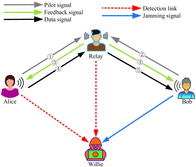
Figure 1: The illustration of two-hop covert relaying system.

In this work we consider a two-hop covert relaying system where Alice $a$ transmits messages to Bob $b$ via a decode-and-forward (DF) relay as Fig. 1 shown. Here, we consider a DF relay since a DF relay can avoid noise propagation and achieve a higher CR [31]. It is assumed that all nodes adopt the half-duplex mode and there is no direct link between $a$ and $b$ due to the path loss and shadowing effects, so the transmission from $a$ to $b$ is divided into two hops, i.e., $a\to r$ transmission (first hop) and $r\to b$ transmission (second hop). Willie $w$ can monitor the transmission of both the first hop and second hop. All channels are subject to independent quasi-static Rayleigh block fading, so the channel coefficient follows an independent and identically distributed (i.i.d.) complex Gaussian distribution with zero mean and unit variance. Thus, we have $h_{ij}\sim CN(0,1)$, where $i$ and $j$ are any two distinct elements of the set $\{a,r,b\}$.

As illustrated in Fig. 2, the covert transmission scheduling in the concerned system is organized into uniformly sized time blocks, where each block is composed of three distinct periods, i.e., a training period, a feedback period, and a data transmission period. During the training period, $a$ and $b$ transmit pilot symbols to $r$ in sequence such that $r$ can estimate the CSIs of both two hops. During the feedback period, $r$ decides whether to engage in covert communication based on the estimated CSIs, then transmits the decision to $a$ and $b$ and the CSI of link $a\to r$ to $a$. Based on the decision, $a$ and $r$ decided to conduct the transmission or keep silent during the data transmission period. It should be noted that to create maximum confusion for $w$, $b$ is required to transmit a jamming signal to disrupt $w$ in the absence of covert transmissions. For clarity, we represent the events of executing covert communication as $H_{1}$ and the absence thereof as $H_{0}$.

II-B The Modeling of Imperfect CSI

In this work, the imperfect CSI encompasses both CEE and FD. To aid in the modeling of the imperfect CSI, $L_{t}$, $L_{f}$, and $L_{d}$ are defined to represent the number of symbols dedicated to training, feedback, and data transmission, respectively. Therefore, the duration of a block is expressed as $L\Delta=(2L_{t}+L_{f}+2L_{d})\Delta$ as depicted in Fig. 2, where $\Delta$ denotes as the duration of one symbol.

During the training period, the received vector of $L_{t}$ pilot symbols at node $j$ is denoted as $\mathbf{y_{j}}={\{y_{j}^{t}\}}\begin{smallmatrix}L_{t}\\ t=1\end{smallmatrix}$, where each $y_{j}^{t}$ is defined as $y_{j}^{t}=\sqrt{P_{t}}{h}_{ij}^{t}x_{i}^{t}+n_{j}^{t}$. Here, $P_{t}$ represents the transmit power of pilot symbols, and $n_{j}^{t}\sim CN(0,N_{0})$ represents the AWGN at $j$. By employing the Minimum Mean Square Error (MMSE) estimation method, the channel gain coefficient without FD can be expressed as

$$h_{ij}^{t}=\hat{h}_{ij}^{t}+e_{ij}^{t},$$ (1)

where $\hat{h}_{ij}$ and $e_{ij}^{t}$ represent the known part and the uncertain part of ${h}_{ij}^{t}$, respectively. According to [32], for a complex Gaussian variable ${h}_{ij}$ with unit variance, $\hat{h}_{ij}$ can be estimated by

$$\hat{h}_{ij}^{t}=\frac{1}{{\|\sqrt{P_{t}}\mathbf{x_{i}}\|}^{2}+N_{0}}\sqrt{P_{t}}\mathbf{x_{i}^{\dagger}}\mathbf{y_{j}}.$$ (2)

By some basic vector operations, the variance of $\hat{h}_{ij}^{t}$ is

$$\mathbb{D}[\hat{h}^{t}_{ij}]=\mathbb{E}[\lvert\hat{h}_{ij}^{t}\rvert^{2}]-\mathbb{E}[\lvert\hat{h}_{ij}^{t}\rvert]^{2}=\frac{P_{t}L_{t}}{P_{t}L_{t}+N_{0}}.$$ (3)

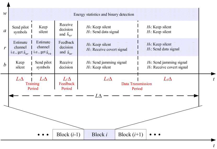
Figure 2: Overall transmission scheduling of the concerned system.

Due to orthogonality principle [33], we square both sides of (1) and take the expectation, getting $\mathbb{E}[\lvert h_{ij}^{t}\rvert^{2}]=\mathbb{E}[\lvert\hat{h}_{ij}^{t}\rvert^{2}]+\mathbb{E}[\lvert e_{ij}^{t}\rvert^{2}]$. Subsequently, we can derive the variance of $e_{ij}^{t}$ for receiver $j$ as

$$\mathbb{D}[e_{ij}^{t}]=\mathbb{E}[\lvert e_{ij}^{t}\rvert^{2}]-\mathbb{E}[\lvert e_{ij}^{t}\rvert]^{2}=\frac{N_{0}}{P_{t}L_{t}+N_{0}}.$$ (4)

It’s worth noting that $\mathbb{D}[e_{ij}^{t}]$ characterizes the channel uncertainty at the receiver $j$, a smaller $\mathbb{D}[e_{ij}^{t}]$ is more advantageous for covert communication. Thus, when both $a$ and $b$ use the maximum transmit power $P_{max}$ to transmit pilot symbols, the optimal variance of $e_{ij}^{t}$, denoted as $\beta^{*}$, can be obtained as

$$\beta^{*}=\frac{N_{0}}{P_{max}L_{t}+N_{0}}.$$ (5)

Due to the time-varying property of the channel, $a$ and $r$ can only rely on the previous channel gain measurements to conduct covert communication. Given that the duration of one symbol is $\Delta$, the time lag from the channel estimation moment is concluded to the transmission of the $t$-th data symbol is expressed as $(L_{f}+t)\Delta$. Consequently, the mean delay for each block is represented by

$$\mathcal{D}=\frac{1}{2L_{d}}\sum_{t=1}^{2L_{d}}(L_{f}+t)\Delta=(\frac{1}{2}+L_{f}+L_{d})\Delta.$$ (6)

Let $\hat{h}_{ij}^{t-\mathcal{D}}$ denote as the time delayed version of $\hat{h}_{ij}^{t}$. Based on the theory of Gauss–Markov process, we can formulate $\hat{h}_{ij}^{t}$ as

$$\hat{h}_{ij}^{t}=\rho_{ij}\hat{h}_{ij}^{t-\mathcal{D}}+\sqrt{1-\rho_{ij}^{2}}\omega_{ij}^{t}$$ (7)

where $\omega_{ij}^{t}$ is a circularly symmetric complex Gaussian random variable (RV) with the same variance as $\hat{h}_{ij}^{t}$, $\rho_{ij}$ is the correlation coefficient (CC) that quantifies the correlation between $\hat{h}_{ij}^{t}$ and $\hat{h}_{ij}^{t-D}$. By using the Jakes’ autocorrelation model, $\rho_{ij}$ is given by $\rho_{ij}=J_{0}(2\pi f_{ij}\mathcal{D})$, where $J_{0}(\textperiodcentered)$ is the zeroth-order Bessel function of the first kind, and $f_{ij}$ is the maximum Doppler frequency for the link $i\to j$.

Now, by integrating (7) into (1), we establish a model that maps the relationship between the instantaneous perfect channel gain coefficient ${h}_{ij}^{t}$, the estimated channel gain at a previous time $\hat{h}_{ij}^{t-\mathcal{D}}$, and the error term $e_{ij}^{t}$ within each block. This relationship is expressed as

$${h}_{ij}^{t}=\rho_{ij}\hat{h}_{ij}^{t-\mathcal{D}}+\sqrt{1-\rho_{ij}^{2}}\omega_{ij}^{t}+e_{ij}^{t}$$ (8)

In the following discussion, we omit the time index $t-\mathcal{D}$ from $\hat{h}_{ij}^{t-\mathcal{D}}$ for the sake of simplicity.

II-C Two-Hop Covert Transmission

In this subsection, we analyze the signal receiving at $r$ and $b$ while conducting two-hop covert transmission.

$\bm{a\to r}$ transmission: $a$ transmits a vector of data symbols $\mathbf{x_{a}}={\{x_{a}^{t}\}}\!\begin{smallmatrix}L_{d}\\ t=1\end{smallmatrix}$ to $r$, where $x_{a}^{t}$ is the $t$-th symbol satisfying $E[\mathbf{x_{a}}\mathbf{x_{a}}^{T}]=1$. Then, the received signal for $r$ is $\mathbf{y_{r}}={\{y_{r}^{t}\}}\!\begin{smallmatrix}L_{d}\\ t=1\end{smallmatrix}$, where $y_{r}^{t}$ is given as

$$y_{r}^{t} =\sqrt{P_{a}}{h}_{ar}^{t}x_{a}^{t}+n_{r}^{t}$$

$$=\sqrt{P_{a}}(\rho_{ar}\hat{h}_{ar}+\sqrt{1-\rho_{ar}^{2}}\omega_{ar}^{t}+e_{ar}^{t})x_{a}^{t}+n_{r}^{t}$$ (9)

where $P_{a}$ is the transmit power at $a$. The imperfect signal-to-interference-noise ratio (SINR) $\tilde{\gamma}_{sr}$ of $\mathbf{x_{a}}$ can be expressed as

$$\tilde{\gamma}_{ar}=\frac{P_{a}\rho_{ar}^{2}\lvert\hat{h}_{ar}\rvert^{2}}{P_{a}((1-\rho_{ar}^{2})\lvert\omega_{ar}^{t}\rvert^{2}+\lvert e_{ar}^{t}\rvert^{2})+N_{0}}$$ (10)

$\bm{r\to b}$ transmission: $r$ forwards a vector of data symbols $\mathbf{x_{r}}={\{x_{r}^{t}\}}\!\begin{smallmatrix}L_{d}\\ t=1\end{smallmatrix}$ to $b$, where $x_{r}^{t}$ is the $t$-th symbol satisfying $E[\mathbf{x_{r}}\mathbf{x_{r}}^{T}]=1$. Thus, the signal received by $b$ is $\mathbf{y_{b}}={\{y_{b}^{t}\}}\!\begin{smallmatrix}L_{d}\\ t=1\end{smallmatrix}$, where $y_{b}^{t}$ is given as

$$y_{d}^{t} =\sqrt{P_{r}}{h}_{rb}^{t}x_{r}^{t}+n_{b}^{t}$$

$$=\sqrt{P_{r}}(\rho_{rd}\hat{h}_{rb}+\sqrt{1-\rho_{rb}^{2}}\omega_{rb}^{t}+e_{rb}^{t})x_{r}^{t}+n_{b}^{t}$$ (11)

where $P_{r}$ represents the transmit power at $r$. Similarly, the imperfect SINR $\tilde{\gamma}_{rb}$ of $\mathbf{x_{r}}$ can be expressed as

$$\tilde{\gamma}_{rb}=\frac{P_{r}\rho_{rb}^{2}\lvert\hat{h}_{rb}\rvert^{2}}{P_{r}((1-\rho_{rb}^{2})\lvert\omega_{rb}^{t}\rvert^{2}+\lvert e_{rb}^{t}\rvert^{2})+N_{0}}.$$ (12)

II-D Willie’s Detection Strategy

As mentioned earlier, $b$ will inject the AN signal to confuse the detection of $w$ in the absence of covert transmission. Thus, we have

$$H_{0}:{y}_{w}^{t}=\sqrt{P_{b}}{h}_{bw}^{t}x_{b}^{t}+n_{w}^{t},$$ (13)

where ${P_{b}}$ and $x_{b}^{t}$ are the jamming symbol and jamming power, respectively. Operating in the half-duplex mode, $r$ is only capable of receiving messages when $a$ is transmitting and cannot send signals simultaneously. Therefore, $w$ can only detect one of the signals from either $a$ or $r$ at any given moment during covert communications. So, we can obtain

$$H_{1}:{y}_{w}^{t}=\sqrt{P_{i}}{h}_{iw}^{t}x_{i}^{t}+n_{w}^{t},$$ (14)

where $i\in\{a,r\}$, $n_{w}^{t}\sim CN(0,N_{0})$ denotes the AWGN at $w$.

$w$ tries to differentiate the events $H_{0}$ and $H_{1}$ by employing a radiometer to measure the received signal power. The decision rule at $w$ follows a rule defined by

$$T_{w}=\frac{1}{L_{w}}\sum_{t=1}^{L_{w}}\lvert{y}_{w}^{t}\rvert^{2}\overset{D_{1}}{\underset{D_{0}}{\gtrless}}\tau$$ (15)

where $L_{w}$ represents the count of observed symbols, $T_{w}$ denotes the mean received power for each $L_{w}$ at $w$, $\tau$ stands as the threshold for judgment, while $D_{1}$ and $D_{0}$ correspond to binary decisions that deduce the presence or absence of covert transmissions in the surrounding environment, respectively.

The detection error probability (DEP) is used to measure the system’s covertness, which can be defined as

$$\xi\overset{\Delta}{=}\mathbb{P}[H_{0}]\times\mathcal{P}_{FA}+\mathbb{P}[H_{1}]\times\mathcal{P}_{MD}.$$ (16)

Here, $\mathbb{P}[H_{0}]$ and $\mathbb{P}[H_{1}]$ represent the prior probabilities of hypotheses $H_{0}$ and $H_{1}$ respectively, while $\mathcal{P}_{FA}=\mathbb{P}[D_{1}|H_{0}]$ signifies the probability of a false alarm, and $\mathcal{P}_{MD}=\mathbb{P}[D_{0}|H_{1}]$ signifies the probability of a miss detection. $w$ intends to select the optimal detection threshold (denoted as $\tau^{*}$) to achieve the minimum DEP (denoted as $\xi^{*}$). The covert requirement for this study is thus defined by the inequality $\xi^{*}\geq\min\{\mathbb{P}[H_{0}],\mathbb{P}[H_{1}]\}-\epsilon$, where $\epsilon$ specifies the required level of covertness.

III PERFORMANCE ANALYSIS

III-A End-to-End Successful Transmission Probability

In this study, we consider that transmitter $i$ utilizes the CIPC scheme, as detailed in [13, 14, 15, 22], for transmitting covert messages. Here, the transmit power $P_{i}$ is adaptively adjusted to maintain a constant $Q_{c}$ where $Q_{c}\overset{\Delta}{=}P_{i}\lvert\hat{h}_{ij}\rvert^{2}$. However, when channel equality is poor, the event that $P_{max}\lvert\hat{h}_{ij}\rvert^{2}<Q_{c}$ may occurs due to the constraint of maximum transmission power. Therefore, the event $H_{1}$ occurs if and only if both conditions $\lvert\hat{h}_{ar}\rvert^{2}P_{max}\geq Q_{c}$ and $\lvert\hat{h}_{rb}\rvert^{2}P_{max}\geq Q_{c}$ are satisfied in the concerned two-hop covert communication. It is deserved to note that transmission outages may still happen even when the channel quality meets the condition of covert communication, where transmission outage is defined as the instantaneous channel capacity $C_{ij}$ is less than the required end-to-end (E2E) transmission rate $R_{b}$.

Overall, we can define the E2E successful transmission probability $\mathcal{P}_{su}$ in this work as the probability that the transmission outage do not occur on either of the two hops under $H_{1}$, i.e., $\mathcal{P}_{su}=\mathbb{P}[(\frac{1}{2}C_{ar}>R_{b}\cap\frac{1}{2}C_{rb}>R_{b})|H_{1}]$. By submitting Eqs. (8), (10) and (12) in it, we can obtain the closed-form of E2E successful transmission probability $\mathcal{P}_{su}$ as the following theorem.

Theorem 1

In the considered two-hop covert relaying system with the imperfect CSI, the E2E successful transmission probability is determined as

$$\mathcal{P}_{su}=\mathcal{P}_{su}^{r}\times\mathcal{P}_{su}^{b},$$ (17)

here $\mathcal{P}_{su}^{r}$ and $\mathcal{P}_{su}^{b}$ are respectively given by

$$\mathcal{P}_{su}^{r}= \begin{cases}\displaystyle 1-{\exp{\{-\phi_{1}\phi_{2}\lambda_{1}\}}\lambda_{3}}\\ \displaystyle\times\frac{\lambda_{3}+\lambda_{1}\phi_{2}(2+\lambda_{1}\phi_{1}\phi_{2}+\lambda_{3}\phi_{1})}{(\lambda_{3}+\lambda_{1}\phi_{2})^{2}},&\lambda_{1}=\lambda_{2}\\ \displaystyle 1+\frac{\exp{\{-\phi_{1}\phi_{2}\lambda_{1}\}}\lambda_{2}\lambda_{3}}{(\lambda_{1}-\lambda_{2})(\lambda_{3}+\lambda_{1}\phi_{2})}\\ \displaystyle+\frac{\exp{\{-\phi_{1}\phi_{2}\lambda_{2}\}}\lambda_{1}\lambda_{3}}{(\lambda_{2}-\lambda_{1})(\lambda_{3}+\lambda_{2}\phi_{2})},&\lambda_{1}\neq\lambda_{2}\end{cases}$$ (18)

$$\mathcal{P}_{su}^{b}= \begin{cases}\displaystyle 1-{\exp{\{-\phi_{1}\phi_{3}\lambda_{4}\}}\lambda_{3}}\\ \displaystyle\times\frac{\lambda_{3}+\lambda_{4}\phi_{3}(2+\lambda_{4}\phi_{1}\phi_{3}+\lambda_{3}\phi_{1})}{(\lambda_{3}+\lambda_{4}\phi_{3})^{2}},&\lambda_{4}=\lambda_{2}\\ \displaystyle 1+\frac{\exp{\{-\phi_{1}\phi_{3}\lambda_{4}\}}\lambda_{2}\lambda_{3}}{(\lambda_{4}-\lambda_{2})(\lambda_{3}+\lambda_{4}\phi_{3})}\\ \displaystyle+\frac{\exp{\{-\phi_{1}\phi_{3}\lambda_{2}\}}\lambda_{4}\lambda_{3}}{(\lambda_{2}-\lambda_{4})(\lambda_{3}+\lambda_{2}\phi_{3})},&\lambda_{4}\neq\lambda_{2}\end{cases}$$ (19)

where $\phi_{1}\overset{\Delta}{=}\frac{Q_{c}}{P_{max}}$, $\phi_{2}\overset{\Delta}{=}\frac{Q_{c}\rho_{ar}^{2}}{4^{R_{ab}}-1}-N_{0}$, $\phi_{3}\overset{\Delta}{=}\frac{Q_{c}\rho_{rb}^{2}}{4^{R_{ab}}-1}-N_{0}$, $\lambda_{1}\overset{\Delta}{=}\frac{1}{Q_{c}(1-\rho_{ar}^{2})(1-\beta^{*})}$, $\lambda_{2}\overset{\Delta}{=}\frac{1}{Q_{c}\beta^{*}}$, $\lambda_{3}\overset{\Delta}{=}\frac{1}{1-\beta^{*}}$, $\lambda_{4}\overset{\Delta}{=}\frac{1}{Q_{c}(1-\rho_{rb}^{2})(1-\beta^{*})}$.

Proof:

With the fact of $C_{ij}=\log_{2}(1+\tilde{\gamma}_{ij})$, we have $\mathcal{P}_{su}=\mathbb{P}[(\frac{1}{2}C_{ar}>R_{b}\cap\frac{1}{2}C_{rb}>R_{b})|H_{1}]=\mathbb{P}[(\log_{2}(1+\tilde{\gamma}_{ar})>2R_{b}\cap\log_{2}(1+\tilde{\gamma}_{rb})>2R_{b})|H_{1}]$. By observation Eq. (10) and Eq.(12), we find the RVs in $\tilde{\gamma}_{ar}$ and ones in $\tilde{\gamma}_{rb}$ are independent. Thus, according to conditional independence in statistics , we can further obtain

$$\mathcal{P}_{su} \!=\!\mathbb{P}[\log_{2}(1\!+\!\tilde{\gamma}_{ar})\!>\!2R_{b}|H_{1}]\times\mathbb{P}[\log_{2}(1\!+\!\tilde{\gamma}_{rb})\!>\!2R_{b}|H_{1}]$$

$$\!=\!\frac{\mathbb{P}[\log_{2}(1\!+\!\tilde{\gamma}_{ar})\!>\!2R_{b},\!H_{1}]}{\mathbb{P}[H_{1}]}\!\times\!\frac{\mathbb{P}[\log_{2}(1\!+\!\tilde{\gamma}_{rb})\!>\!2R_{b},\!H_{1}]}{\mathbb{P}[H_{1}]}.$$ (20)

We first derive the probability $\mathbb{P}[H_{1}]$ of conducting covert communication as follows

$$\mathbb{P}[H_{1}]=\mathbb{P}[\lvert\hat{h}_{ar}\rvert^{2}P_{max}>Q_{c},\lvert\hat{h}_{rb}\rvert^{2}P_{max}>Q_{c}]$$

$$=\!\!\int\nolimits_{\phi_{1}}^{\infty}\!\!\lambda_{3}\exp\{-\lambda_{3}\lvert\hat{h}_{ar}\rvert^{2}\}d\lvert\hat{h}_{ar}\rvert^{2}\!\!\int\nolimits_{\phi_{1}}^{\infty}\!\!\lambda_{3}\exp\{-\lambda_{3}\lvert\hat{h}_{rb}\rvert^{2}\}d\lvert\hat{h}_{rb}\rvert^{2}$$

$$=\exp{\Big{\{}\frac{-2Q_{c}}{P_{max}(1-\beta^{*})}\Big{\}}}\overset{\Delta}{=}\theta.$$ (21)

Accordingly, the probability $\mathbb{P}[H_{0}]$ that the system does not execute covert communication is given by $\mathbb{P}[H_{0}]=1-\mathbb{P}[H_{1}]=1-\theta$.

Then, the numerator of the first term on the right side of Eq. (III-A) can be derived as

$$\mathbb{P}[\log_{2}(1+\tilde{\gamma}_{ar})>2R_{b},H_{1}]$$

$$=\mathbb{P}[\log_{2}(1\!+\!\tilde{\gamma}_{ar})\!>\!2R_{b},\lvert\hat{h}_{ar}\rvert^{2}P_{max}\!>\!Q_{c},\lvert\hat{h}_{rb}\rvert^{2}P_{max}\!>\!Q_{c}]$$

$$=\mathbb{P}\bigg{[}\lvert\hat{h}_{ar}\rvert^{2}P_{max}>Q_{c},\lvert\hat{h}_{rb}\rvert^{2}P_{max}>Q_{c},$$

$$\quad\quad\frac{P_{a}\rho_{ar}^{2}\lvert\hat{h}_{ar}\rvert^{2}}{P_{a}((1-\rho_{ar}^{2})\lvert\omega_{ar}^{t}\rvert^{2}+\lvert e_{ar}^{t}\rvert^{2})+N_{0}}>4^{R_{b}}-1\bigg{]}$$ (22)

For convenience of expression, we define $x_{1}\overset{\Delta}{=}Q_{c}(1-\rho_{ar}^{2})\lvert\omega_{ar}^{t}\rvert^{2}$, $x_{2}\overset{\Delta}{=}Q_{c}\lvert e_{ar}^{t}\rvert^{2}$, $x_{3}\overset{\Delta}{=}\lvert\hat{h}_{ar}\rvert^{2}$, and $x_{4}\overset{\Delta}{=}\lvert\hat{h}_{rb}\rvert^{2}$ in Eq. (22). According to the description of $\omega_{ij}^{t}$, $e_{ij}^{t}$ and $\hat{h}_{ij}$ in Section II, we can easily get $x_{1}\sim\text{EXP}(\lambda_{1})$, $x_{2}\sim\text{EXP}(\lambda_{2})$, $x_{3}\sim\text{EXP}(\lambda_{3})$, and $x_{4}\sim\text{EXP}(\lambda_{3})$. Thus, Eq. (22) can be further simplified as follows

$$\mathbb{P}[\log_{2}(1+\tilde{\gamma}_{ar})>2R_{b},H_{1}]$$

$$=\mathbb{P}\bigg{[}\frac{Q_{c}\rho_{ar}^{2}}{(x_{1}+x_{2})/x_{3}+N_{0}}>4^{R_{ab}}-1,x_{3}>\phi_{1},x_{4}>\phi_{1}\bigg{]},$$

$$=\int\nolimits_{\phi_{1}}^{\infty}\int\nolimits_{\phi_{1}}^{\infty}{\lambda_{3}}^{2}\exp\{-\lambda_{3}(x_{3}+x_{4})\}$$

$$\times\!\int\nolimits_{0}^{\phi_{2}x_{3}}\!\!\!\int\nolimits_{0}^{\phi_{2}x_{3}-x_{2}}\!\!{\lambda_{2}}{\lambda_{1}}\exp\{-\lambda_{2}x_{2}-\lambda_{1}x_{1}\}dx_{1}dx_{2}dx_{3}dx_{4}$$ (23)

After performing some integral operations, $\mathbb{P}[\log_{2}(1+\tilde{\gamma}_{ar})>2R_{b},H_{1}]$ can be calculated as Eq. (24). Subsequently, incorporating Eq. (21) and Eq.(24) ( into the first term on the right side of Eq. (III-A), we derive that this term is equivalent to $\mathcal{P}^{r}_{su}$ (i.e., Eq. (18)). Similarly, we can obtain the second term on the right side of Eq. (III-A) as $\mathcal{P}^{b}_{su}$ (i.e., Eq. (19)). ∎

$$\mathbb{P}[\log_{2}(1+\tilde{\gamma}_{ar})>2R_{b},H_{1}]=\begin{cases}\displaystyle\theta-\theta{\exp{\{-\phi_{1}\phi_{2}\lambda_{1}\}}\lambda_{3}}\times\frac{\lambda_{3}+\lambda_{1}\phi_{2}(2+\lambda_{1}\phi_{1}\phi_{2}+\lambda_{3}\phi_{1})}{(\lambda_{3}+\lambda_{1}\phi_{2})^{2}},&\lambda_{1}=\lambda_{2}\\ \displaystyle\theta+\frac{\theta\exp{\{-\phi_{1}\phi_{2}\lambda_{1}\}}\lambda_{2}\lambda_{3}}{(\lambda_{1}-\lambda_{2})(\lambda_{3}+\lambda_{1}\phi_{2})}+\frac{\theta\exp{\{-\phi_{1}\phi_{2}\lambda_{2}\}}\lambda_{1}\lambda_{3}}{(\lambda_{2}-\lambda_{1})(\lambda_{3}+\lambda_{2}\phi_{2})},&\lambda_{1}\neq\lambda_{2}\end{cases}$$ (24)

Through a detailed analysis of the expression for $P_{su}$, the following corollary can be deduced.

Corollary 1

When the data symbol length $L_{d}$ is less than $L_{d}^{max}$, the E2E successful transmission probability $\mathcal{P}_{su}$ monotonically decreases with respect to $L_{d}$, the maximal data symbol length is determined as

$$L_{d}^{max}\overset{\Delta}{=}\Big{\lfloor}\frac{\psi_{0}}{2\pi\max{\{f_{ar},f_{rb}\}}\Delta}-L_{f}-\frac{1}{2}\Big{\rfloor}.$$ (25)

where $\psi_{0}$ is a constant that satisfies $\lvert J_{0}(\psi_{0})\rvert=\lvert J_{0}(\psi_{1})\rvert$, with $\psi_{0}$ being less than $\psi_{1}$, which represents the x-coordinate of the first trough in $J_{0}(x)$. The approximate value of $\psi_{0}$ is determined to be $1.6918$ through numerical solution.

Proof:

Since $\mathcal{P}_{su}$ is the product of $\mathcal{P}^{r}_{su}$ and $\mathcal{P}^{b}_{su}$, as indicated in (17), our initial analysis focuses on the monotonicity of $\mathcal{P}^{r}_{su}$ with respect to $L_{d}$. Since $\mathcal{P}^{r}_{su}$ is a piecewise function as Eq. (18), we conduct the analysis from the following two cases.

Case 1 ($\lambda_{1}=\lambda_{2}$): According to Subsection II-B, $\rho_{ar}^{2}$ is a function of $L_{D}$. Therefore, to analyze the monotonicity of $\mathcal{P}^{r}_{su}$ with respect to $L_{d}$, we first derive the first-order derivative of $\mathcal{P}_{su}^{r}$ with respect to $\rho_{ar}^{2}$ as follows

$$\frac{\partial\mathcal{P}_{su}^{r}}{\partial\rho_{ar}^{2}} =\frac{\partial\mathcal{P}_{su}^{r}}{\partial z_{1}}\times\frac{\partial z_{1}}{\partial\rho_{ar}^{2}}$$

$$=\frac{\lambda_{3}(2+2\phi_{1}(\lambda_{3}+z_{1})+\phi_{1}^{2}(\lambda_{3}+z_{1})^{2})}{e^{\phi_{1}}(\lambda_{3}+z_{1})^{3}}$$

$$\quad\times\frac{N_{0}(1-4^{R_{ab}})+Q_{c}}{(4^{R_{ab}}-1)(1-\beta)(1-\rho_{ar}^{2})^{2}Q_{c}}$$ (26)

where $z_{1}\overset{\Delta}{=}\lambda_{1}\phi_{2}$. Easily, we can obtain that $\frac{\partial\mathcal{P}_{su}^{r}}{\partial\rho_{ar}^{2}}>0$, such that the monotonicity of $\mathcal{P}^{r}_{su}$ with respect to $L_{d}$ depends on the monotonicity of $\rho_{ar}^{2}$ with respect to $L_{d}$.

It is well-known that the Bessel function is not a monotonic function; hence, its square, $y_{2}=\rho_{ar}^{2}={J_{0}^{2}(x)}$, is also non-monotonic, as illustrated in Fig. 3. We observe that the heights of the peaks of $y_{2}$ function decrease sequentially, with the x-coordinate of the $k$-th peak denoted by $\psi_{k}$ (e.g. $\psi_{1}=3.8345$, $\psi_{2}=7.0163$) [35]. We define a point $\psi_{0}$, which satisfies ${J_{0}^{2}(\psi_{0})}$ being equal to the height of the first peak of the $y_{2}$ function, ${J_{0}^{2}(\psi_{1})}$ (i.e., $\lvert J_{0}(\psi_{0})\rvert=\lvert J_{0}(\psi_{1})\rvert$), and also meets the condition $\psi_{0}<\psi_{1}$. This allows us to conclude that within the interval [0, $\psi_{0}$], the $y_{2}$ function is monotonically decreasing. The approximate value of $\psi_{0}$ is determined to be $1.6918$ through numerical solution.

Then, by plugging $L_{d}=2\pi f_{ar}\mathcal{D}$ into these intervals, we get the following inequalities

$$x=2\pi f_{ar}(\frac{1}{2}+L_{f}+L_{d})\Delta\leq\psi_{0}$$ (27)

By simplifying the above inequality, and considering that $L_{d}$ must be an integer, we can further obtain the following inequality

$$L_{d}\leq\Big{\lfloor}\frac{\psi_{0}}{2\pi f_{ar}\Delta}-L_{f}-\frac{1}{2}\Big{\rfloor}$$ (28)

Therefore, we can get that $\rho_{ar}^{2}$ is a monotonic decreasing function when $L_{d}\in[0,\lfloor\frac{\psi_{0}}{2\pi f_{ar}\Delta}-L_{f}-\frac{1}{2}\rfloor]$.

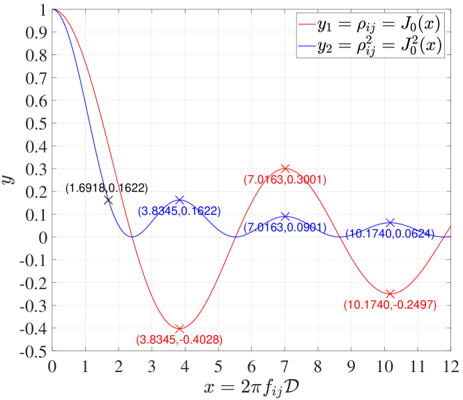
Figure 3: Overall transmission scheduling of the concerned system.

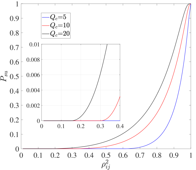
Figure 4: Successful transmission probability $\mathcal{P}_{su}$ vs. $\rho_{ar}^{2}$ with $P_{max}=20$dBm, $N_{0}=0$dBm.

Case 2 ($\lambda_{1}\neq\lambda_{2}$): Obviously, $\mathbb{P}[H_{1}]$ is no related with $L_{d}$. Hence, in this case, we can equally analyze the monotonicity of $\mathbb{P}[\tilde{\gamma}_{ar}>4^{R_{ab}}-1,H_{1}]$ with respect to $L_{d}$. From Eq. (10), we can see that $\tilde{\gamma}_{ar}$ is an increasing function with respect to $\rho_{ar}^{2}$, i.e, $\frac{\partial\mathcal{P}_{su}^{r}}{\partial\rho_{ar}^{2}}>0$. Therefore, the analysis degenerates into the monotonicity analysis of $\rho_{ar}^{2}$ with respect to $L_{d}$, which is same with the Case 1.

Symmetrically, we can obtain that $\mathcal{P}^{b}_{su}$ is a monotonic decreasing function when $0\leq L_{d}\leq\lfloor\frac{\psi_{0}}{2\pi f_{rb}\Delta}-L_{f}-\frac{1}{2}\rfloor$. The proof is similar with one of $\mathcal{P}^{r}_{su}$, we omit here. In summary, $\mathcal{P}_{su}$ monotonically decreases with respect to $L_{d}$ for $L_{d}\in[0,\lfloor\frac{\psi_{0}}{2\pi\max{\{f_{ar},f_{rb}\}}\Delta}-L_{f}-\frac{1}{2}\rfloor]$.

Note that the monotonicity of $P_{su}$ for $x>\psi_{0}$ (i.e., $L_{d}>\lfloor\frac{\psi_{0}}{2\pi\max{\{f_{ar},f_{rb}\}}\Delta}-L_{f}-\frac{1}{2}\rfloor$) is not considered here. As Fig. 4 shown, when $x>\psi_{0}$, ${J_{0}^{2}(x)}\leq 0.1622$, $P_{su}$ is less than $0.2\%$, which means that only a tiny fraction of the transmitted data can be successfully decoded. Thus, it is not particularly meaningful to analyze the case.

∎

III-B Derivation of Detection Error Probability

In the concerned system, $w$ makes a binary judgment after collecting the energy of $L_{w}$ symbols. By substituting (13) and (14) into (15) and combining the transmission scheduling described in Fig. 2, we have the average received power $T_{w}$ under $H_{0}$ and $H_{1}$ as

$$T_{w}=\begin{cases}\frac{1}{L_{w}}\Big{(}\sum\limits_{t=1}^{L_{w}L_{t}/L}\!P_{max}\lvert{h}_{aw}^{t}\rvert^{2}+\sum\limits_{t=1}^{L_{w}L_{t}/L}\!P_{max}\lvert{h}_{bw}^{t}\rvert^{2}\\ +\!\sum\limits_{t=1}^{L_{w}L_{f}/L}P_{max}\lvert{h}_{rw}^{t}\rvert^{2}+\sum\limits_{t=1}^{2L_{w}L_{d}/L}P_{b}\lvert{h}_{bw}^{t}\rvert^{2}\\ +\sum\limits_{t=1}^{L_{w}}\lvert n_{w}^{t}\rvert^{2}\Big{)},&H_{0}\\ \frac{1}{L_{w}}\Big{(}\sum\limits_{t=1}^{L_{w}L_{t}/L}\!P_{max}\lvert{h}_{aw}^{t}\rvert^{2}+\sum\limits_{t=1}^{L_{w}L_{t}/L}\!P_{max}\lvert{h}_{bw}^{t}\rvert^{2}\\ +\!\sum\limits_{t=1}^{L_{w}L_{f}/L}P_{max}\lvert{h}_{rw}^{t}\rvert^{2}+\sum\limits_{t=1}^{L_{w}L_{d}/L}P_{a}\lvert{h}_{aw}^{t}\rvert^{2}\\ +\sum\limits_{t=1}^{L_{w}L_{d}/L}P_{r}\lvert{h}_{rw}^{t}\rvert^{2}+\sum\limits_{t=1}^{L_{w}}\lvert n_{w}^{t}\rvert^{2}\Big{)},&H_{1}\end{cases}$$ (29)

$w$ makes a binary judgment after collecting energy for a long time. This long time contains numerous messages of covert communication, each containing $L$ symbols, so it is reasonable to assume that $w$ observed an infinite number of symbols for each judgment, i.e., $L_{w}\to\infty$.

As per (16), to get the closed-form result of DEP, we first need to derive $\mathcal{P}_{FA}$ and $\mathcal{P}_{MD}$. According to their definitions, by analyzing the received signals for $H_{0}$ and $H_{1}$ at $w$, and comparing them with the given detection threshold $\tau$, we can obtain $\mathcal{P}_{FA}$ and $\mathcal{P}_{MD}$ which is given by the following theorem.

Theorem 2

For a given $\tau$ at $w$, $\mathcal{P}_{FA}$ and $\mathcal{P}_{MD}$ under the CIPC scheme with the imperfect CSIs can be given by

$$\mathcal{P}_{FA}=\begin{cases}1,&N_{0}+\phi_{4}>\tau\\ e^{\nu_{1}(\tau)},&\tau\geq\ N_{0}+\phi_{4}\end{cases}$$ (30)

$$\mathcal{P}_{MD}\!=\!\begin{cases}0,&\!\!\!\!\!\!\!\!\!\!\!\!\!\!\!\!\!\!\!\!\!\!\!\!\!\!\!\!N_{0}+\phi_{4}>\tau\\ \displaystyle\frac{2\big{[}\lambda_{3}^{2}\big{(}\nu_{3}(\tau)\phi_{1}+1\big{)}\nu_{4}(\tau)-\lambda_{3}\nu_{3}(\tau)\big{]}}{e^{\nu_{2}(\tau)\phi_{1}}\nu_{3}^{2}(\tau)}+1,\\ &\!\!\!\!\!\!\!\!\!\!\!\!\!\!\!\!\!\!\!\!\!\!\!\!\!\!\!\!\tau\geq\ N_{0}+\phi_{4}\end{cases}$$ (31)

where $\lambda_{3}$ refer to Theorem 1, $\phi_{4}\overset{\Delta}{=}\frac{P_{max}(L-2L_{d})}{L}$, functions of detection threshold $\nu_{1}(\tau)$, $\nu_{2}(\tau)$, $\nu_{3}(\tau)$ and $\nu_{4}(\tau)$ are given by, respectively,

$$\nu_{1}(\tau)\overset{\Delta}{=}\frac{L(N_{0}-\tau)}{L_{d}P_{max}}$$ (32)

$$\nu_{2}(\tau)\overset{\Delta}{=}\frac{L(\tau-N_{0}-\phi_{4})}{L_{d}Q_{c}}.$$ (33)

$$\nu_{3}(\tau)\overset{\Delta}{=}\nu_{2}(\tau)+2\lambda_{3}$$ (34)

$$\nu_{4}(\tau)\overset{\Delta}{=}\ln\Big{(}\frac{\lambda_{3}}{\lambda_{3}+\nu_{2}(\tau)}\Big{)}$$ (35)

Proof:

According to $T_{w}$ under $H_{0}$ in (29), when $L_{w}\to\infty$, the false alarm probability $\mathcal{P}_{FA}$ can be calculated as

$$\mathcal{P}_{FA}=\mathbb{P}(D_{1}|H_{0})=\mathbb{P}\Big{[}\lim\limits_{L_{w}\to\infty}T_{w}>\tau|H_{0}\Big{]}$$

$$=\mathbb{P}\Big{[}\frac{P_{max}L_{t}}{L}\lvert{h}_{aw}^{t}\rvert^{2}+\frac{P_{max}L_{t}}{L}\lvert{h}_{bw}^{t}\rvert^{2}+\frac{P_{max}L_{f}}{L}\lvert{h}_{rw}^{t}\rvert^{2}$$

$$+\frac{2L_{d}}{L}P_{b}\lvert{h}_{bw}^{t}\rvert^{2}+N_{0}>\tau\Big{]}$$ (36)

We know $L_{t}$ and $L_{f}$ are much smaller than $L_{d}$, so we use their expectations to represent the random variables containing $L_{t}$ and $L_{f}$ items to facilitate the derivation. Due to $\mathbb{E}[\lvert{h}_{aw}^{t}\rvert^{2}]=\mathbb{E}[\lvert{h}_{rw}^{t}\rvert^{2}]=\mathbb{E}[\lvert{h}_{bw}^{t}\rvert^{2}]=1$, we have the approximated form for $\mathcal{P}_{FA}$

$$\mathcal{P}_{FA}\approx\mathbb{P}\Big{[}\phi_{4}+\frac{2L_{d}}{L}P_{b}\lvert{h}_{bw}^{t}\rvert^{2}+N_{0}>\tau\Big{]}$$ (37)

When $\tau<N_{0}+\phi_{4}$, $\mathcal{P}_{FA}=1$, and when $\tau\geq N_{0}+\phi_{4}$, we have

$$\mathcal{P}_{FA} =\int\nolimits_{\frac{L(\tau-N_{0}-\phi_{4})}{2L_{d}P_{b}}}^{\infty}\exp{\{-\lvert{h}_{bw}^{t}\rvert^{2}\}}d\lvert{h}_{bw}^{t}\rvert^{2}$$

$$=\exp{\Big{\{}\frac{L(N_{0}+\phi_{4}-\tau)}{L_{d}P_{max}}\Big{\}}}$$ (38)

On the other side, according to $T_{w}$ under $H_{1}$ in (29), when $L_{w}\to\infty$, the miss detection probability $\mathcal{P}_{MD}$ can be expressed as

$$\mathcal{P}_{MD}=\mathbb{P}(D_{0}|H_{1})=\mathbb{P}\Big{[}\lim\limits_{L_{w}\to\infty}T_{w}<\tau|H_{1}\Big{]}$$

$$=\mathbb{P}\Big{[}\frac{P_{max}L_{t}}{L}\lvert{h}_{aw}^{t}\rvert^{2}+\frac{P_{max}L_{t}}{L}\lvert{h}_{bw}^{t}\rvert^{2}+\frac{P_{max}L_{f}}{L}\lvert{h}_{rw}^{t}\rvert^{2}$$

$$+\frac{Q_{c}L_{d}}{L}\frac{\lvert{h}_{aw}^{t}\rvert^{2}}{\lvert\hat{h}_{ar}\rvert^{2}}+\frac{Q_{c}L_{d}}{L}\frac{\lvert{h}_{rw}^{t}\rvert^{2}}{\lvert\hat{h}_{rb}\rvert^{2}}+N_{0}<\tau,H_{1}\Big{]}/\mathbb{P}(H_{1}).$$ (39)

Similar to the approximated $\mathcal{P}_{FA}$, we have the approximated form for $\mathcal{P}_{MD}$

$$\mathcal{P}_{MD}\approx\mathbb{P}\Big{[}\phi_{4}+\frac{Q_{c}L_{d}\lvert{h}_{aw}^{t}\rvert^{2}}{L\lvert\hat{h}_{ar}\rvert^{2}}+\frac{Q_{c}L_{d}\lvert{h}_{rw}^{t}\rvert^{2}}{L\lvert\hat{h}_{rb}\rvert^{2}}+N_{0}<\tau|H_{1}\Big{]}$$

$$=\mathbb{P}\Big{[}\frac{\lvert{h}_{aw}^{t}\rvert^{2}}{\lvert\hat{h}_{ar}\rvert^{2}}+\frac{\lvert{h}_{rw}^{t}\rvert^{2}}{\lvert\hat{h}_{rb}\rvert^{2}}<\nu_{2}(\tau),H_{1}\Big{]}/\mathbb{P}(H_{1})$$ (40)

We know that $\lvert h^{t}_{aw}\rvert^{2}\sim\text{EXP}(1)$ and $\lvert h^{t}_{rw}\rvert^{2}\sim\text{EXP}(1)$. Moreover, due to $\hat{h}_{ij}\sim CN(0,1-\beta_{j})$, we have $\lvert\hat{h}_{ar}\rvert^{2}\sim\text{EXP}(\lambda_{3})$ and $\lvert\hat{h}_{rb}\rvert^{2}\sim\text{EXP}(\lambda_{3})$. If $\nu_{2}(\tau)<0$. i.e.,$\tau<N_{0}+\phi_{4}$, $\mathcal{P}_{MD}=0$; And if $\nu_{2}(\tau)>0$. i.e.,$\tau\geq N_{0}+\phi_{4}$, by defining $y_{1}\overset{\Delta}{=}\lvert{h}_{aw}^{t}\rvert^{2}$, $y_{2}\overset{\Delta}{=}\lvert\hat{h}_{ar}\rvert^{2}$, $y_{3}\overset{\Delta}{=}\lvert{h}_{rw}^{t}\rvert^{2}$ and $y_{4}\overset{\Delta}{=}\lvert\hat{h}_{rb}\rvert^{2}$, $\mathcal{P}_{MD}\times\mathbb{P}(H_{1})$ is calculated in (41) as follows

$$\mathcal{P}_{MD}\times\mathbb{P}(H_{1})=\mathbb{P}\Big{[}\frac{y_{1}}{y_{2}}+\frac{y_{3}}{y_{4}}<\nu_{2}(\tau),H_{1}\Big{]}$$

$$=\int\nolimits_{\phi_{1}}^{\infty}\lambda_{3}e^{-\lambda_{3}y_{4}}\int\nolimits_{0}^{\nu_{2}(\tau)y_{4}}e^{-y_{3}}\int\nolimits_{\phi_{1}}^{\infty}\lambda_{3}e^{-\lambda_{3}y_{2}}$$

$$\!\!\!\!\!\quad\quad\int\nolimits_{0}^{\big{(}\nu_{2}(\tau)-\frac{y_{3}}{y_{4}}\big{)}y_{2}}e^{-y_{1}}dy_{1}dy_{2}dy_{3}dy_{4}$$

$$\stackrel{{\scriptstyle a}}{{=}}\theta+\frac{e^{-\nu_{3}(\tau)\phi_{1}}}{\nu_{3}^{2}(\tau)}\Bigg{[}2\lambda_{3}^{2}\Big{(}1+\nu_{3}(\tau)\phi_{1}\Big{)}\nu_{4}(\tau)-2\lambda_{3}\nu_{3}(\tau)\Bigg{]}$$ (41)

where $a$ implies that the fourfold integral can be sequentially solved according to the specified order of integration from the innermost to the outermost variable. Substituting (21) and (41) into (40), (31) is achieved. ∎

According to Theorem 35 and the defination of DEP in (16), we can get the following theorem about the DEP at $w$.

Theorem 3

The DEP at $w$ in the concerned system with the imperfect CSI can be given by

$$\xi=\begin{cases}1-\theta,&\!\!\!\!\!\!\!\!\!\!\!\!\!\!\!\!\!\!\phi_{4}+N_{0}>\tau\\ \displaystyle\frac{2\big{[}\lambda_{3}^{2}\big{(}\nu_{3}(\tau)\phi_{1}+1\big{)}\nu_{4}(\tau)-\lambda_{3}\nu_{3}(\tau)\big{]}}{e^{\nu_{3}(\tau)\phi_{1}}\nu_{3}^{2}(\tau)}\\ +\theta+e^{\nu_{1}(\tau)}(1-\theta),&\!\!\!\!\!\!\!\!\!\!\!\!\!\!\!\!\!\!\tau\geq\phi_{4}+N_{0}\\ \theta,&\!\!\!\!\!\!\!\!\!\!\!\!\!\!\!\!\!\!\tau\to\infty\end{cases}$$ (42)

where each of these symbols has been defined in Theorem 1 and Theorem 35.

Proof:

Substituting (21), (30) and (31) into (16), the first two cases of (42) can be achieved. Then we consider the last case of $\tau\to\infty$. For facility of analysis, we denote this case as

$$\xi =\lim\limits_{\tau\to\infty}\frac{2\lambda_{3}^{2}\phi_{1}\nu_{4}(\tau)}{e^{\nu_{3}(\tau)\phi_{1}}\nu_{3}(\tau)}+\lim\limits_{\tau\to\infty}\frac{2\lambda_{3}^{2}\nu_{4}(\tau)}{e^{\nu_{3}(\tau)\phi_{1}}\nu_{3}^{2}(\tau)}$$

$$+\lim\limits_{\tau\to\infty}\frac{-2\lambda_{3}}{e^{\nu_{3}(\tau)\phi_{1}}\nu_{3}(\tau)}+\theta+\lim\limits_{\tau\to\infty}e^{\nu_{1}(\tau)}(1-\theta)$$ (43)

As $\tau$ approaches infinity, $\nu_{1}(\tau)$ and $\nu_{4}(\tau)$ tend towards negative infinity, while both $\nu_{2}(\tau)$ and $\nu_{3}(\tau)$ tend towards positive infinity. It can be easily obtained that the third and fifth terms are zero. Since both the numerator and denominator of the first item approach infinity, applying l’Hôpital’s rule yields

$$\lim\limits_{\tau\to\infty}\frac{[2\lambda_{3}^{2}\phi_{1}\nu_{4}(\tau)]^{\prime}}{[e^{\nu_{3}(\tau)\phi_{1}}\nu_{3}(\tau)]^{\prime}}=\lim\limits_{\tau\to\infty}\frac{2\lambda_{3}\phi_{1}(\nu_{3}(\tau)-\lambda_{3})}{e^{\nu_{3}(\tau)\phi_{1}}(\nu_{3}(\tau)+1)}=0$$ (44)

Thus, the first term of (43) is zero. Similarly, we get that the second term is also zero. So $\xi=\theta$ in the case of $\tau\to\infty$. ∎

According to (42), when $\tau>\phi_{4}+N_{0}$, the first-order derivative of $\xi$ with respect to $\tau$ is too complicated to judge its positive or negative, so we use the numerical search to find the local optimal $\tau$ in this interval, and the global optimal $\tau$ can be given by

$$\tau^{*}\overset{\Delta}{=} \operatorname*{argmin}_{\tau\geq\ \phi_{4}+N_{0}}\theta+e^{\nu_{1}(\tau)}(1-\theta)+e^{-\nu_{3}(\tau)\phi_{1}}\times$$

$$\frac{2\big{[}\lambda_{3}^{2}\big{(}\nu_{3}(\tau)\phi_{1}+1\big{)}\nu_{4}(\tau)-\lambda_{3}\nu_{3}(\tau)\big{]}}{\nu_{3}^{2}(\tau)}.$$ (45)

Note that no upper bound for $\tau$ is given in (45). Though we know that $\tau$ does not need to set very large, because DEP tends to $\theta$ as $\tau$ tends to infinity. We still hope to find a specific upper bound of $\tau$. So we use a compact lower bound function of DEP as follows.

Lemma 1

When $\tau\geq\phi_{4}+N_{0}$, a compact lower bound function of DEP can be given by

$$\xi_{lb}=\theta-e^{\nu_{1}(\tau)}\times\Big{[}e^{\phi_{5}}\times\nu_{5}(\tau)-1+\theta\Big{]}$$ (46)

where $\phi_{5}\overset{\Delta}{=}\frac{L-2L_{d}}{L_{d}}-\frac{2\lambda_{3}Q_{c}}{P_{max}}$, the function of detection threshold $\nu_{5}(\tau)$ is given by,

$$\nu_{5}(\tau)\overset{\Delta}{=}\frac{2\lambda_{3}\big{(}\phi_{1}\nu_{2}(\tau)\nu_{3}(\tau)+\nu_{2}(\tau)+\nu_{3}(\tau)\big{)}}{\nu_{3}^{2}(\tau)}.$$ (47)

Proof:

Because the logarithmic operation is more complicated, we eliminate the logarithm-containing term in (42) by finding the approximate lower bound of the $\nu_{4}(\tau)$ function, which is given by

$$\nu_{6}(\tau)\overset{\Delta}{=}-\frac{\nu_{2}(\tau)}{\lambda_{3}}$$ (48)

When $\tau=\phi_{4}+N_{0}$, $\nu_{2}(\tau)=0$, so $\nu_{4}(\tau)=\nu_{6}(\tau)=0$. Next, use the derivative function to judge the increase and decrease trends of $\nu_{4}(\tau)$ and $\nu_{6}(\tau)$ when $\tau\geq\phi_{4}+N_{0}$.

$$\frac{\partial\nu_{4}(\tau)}{\partial\tau}=-\frac{1}{\lambda_{3}+\nu_{2}(\tau)}\times\frac{L}{L_{d}Q_{c}},$$ (49)

$$\frac{\partial\nu_{6}(\tau)}{\partial\tau}=-\frac{1}{\lambda_{3}}\times\frac{L}{L_{d}Q_{c}},$$ (50)

when $\tau>\phi_{4}+N_{0}$, $\nu_{2}(\tau)>0$, so $\frac{\partial\nu_{4}(\tau)}{\partial\tau}>\frac{\partial\nu_{6}(\tau)}{\partial\tau}$. So when $\tau\geq\phi_{4}+N_{0}$, $\nu_{4}(\tau)\geq\nu_{6}(\tau)$. In addition, we can see that in (42), DEP $\xi$ decreases with the decrease of $\nu_{4}(\tau)$, so after replacing $\nu_{4}(\tau)$ with $\nu_{6}(\tau)$ in (42) and some basic calculations, the lower bound of $\xi$ will be obtained as in (46). ∎

The reason for using the lower bound of DEP instead of the upper bound is that our work considers the worst-case, when the covertness constraint satisfies the lower bound function of DEP, it is more satisfied with the original function of DEP, i.e., $\forall\tau\big{(}\xi_{lb}(\tau)\geq\min\{\mathbb{P}[H_{0}],\mathbb{P}[H_{1}]\}-\epsilon\big{)}\to\forall\tau\big{(}\xi(\tau)\geq\min\{\mathbb{P}[H_{0}],\mathbb{P}[H_{1}]\}-\epsilon$).

With the aid of Lemma 1, we can identify the optimal detection threshold $\tau$ in the tight lower bound function of DEP, as demonstrated in the following theorem.

Theorem 4

The global optimal $\tau$ for $\xi_{lb}$ can be given by

$$\tau^{*}\overset{\Delta}{=}\operatorname*{argmin}_{\tau_{max}\geq\ \tau\geq\ \tau_{min}}\theta-e^{\nu_{1}(\tau)}\times$$

$$\Big{[}e^{\phi_{5}}\times\frac{2\lambda_{3}\big{(}\phi_{1}\nu_{2}(\tau)\nu_{3}(\tau)+\nu_{2}(\tau)+\nu_{3}(\tau)\big{)}}{\nu_{3}^{2}(\tau)}-1+\theta\Big{]}.$$ (51)

where the lower and upper bound of the optimal $\tau$ is given by, respectively,

$$\tau_{min}\overset{\Delta}{=}\phi_{4}+N_{0}=\frac{P_{max}(L-2L_{d})}{L}+N_{0},$$ (52)

$$\tau_{max}\overset{\Delta}{=}\frac{2L_{d}(\lambda_{3}^{2}Q_{c}^{2}+\lambda_{3}P_{max}Q_{c}-P_{max}^{2})}{L(P_{max}-\lambda_{3}Q_{c})}+P_{max}+N_{0}.$$ (53)

Proof:

According to (45), we already know the lower bound of the optimal $\tau$, i.e., $\tau^{*}\in[\phi_{4}+N_{0},\infty)$. To further prove the upper bound of the optimal $\tau$, we need to verify $\xi_{lb}$ in (46) is a increasing function of $\tau$, $\forall\tau>\tau_{max}$.

We note that $e^{\nu_{1}(\tau)}$ is a decreasing function of $\tau$, and when $\tau>\phi_{4}+N_{0}$, both $e^{\nu_{1}(\tau)}$ and $\Big{[}e^{\phi_{5}}\times\nu_{5}(\tau)-1+\theta\Big{]}$ are positive values. So when $\nu_{5}(\tau)$ also is a decreasing function of $\tau$, the $\xi_{lb}$ would be a increasing function of $\tau$. The first-order derivative of $\nu_{5}(\tau)$ with respect to $\tau$ is given as

$$\frac{\partial\nu_{5}(\tau)}{\partial\tau}=$$

$$\frac{4L\lambda_{3}L_{d}Q_{c}(2\lambda_{3}^{2}L_{d}Q_{c}\phi_{1}-L(\lambda_{3}\phi_{1}-1)(\phi_{4}+N_{0}-\tau))}{\big{(}L(\phi_{4}+N_{0}-\tau)-2\lambda_{3}L_{d}Q_{c}\big{)}^{3}},$$ (54)

Let equation (54) equals to zero and combining the definition of $\phi_{1}$ and $\phi_{4}$, we can obtain $\tau=\tau_{max}$. By substituting the point $\tau=\phi_{4}+N_{0}$, we further obtain $\partial\nu_{5}(\tau)/\partial\tau<0$ if $\tau<\tau_{max}$ and $\partial\nu_{5}(\tau)/\partial\tau>0$ if $\tau>\tau_{max}$. Thus, we proved $\xi_{lb}$ in (46) is a increasing function of $\tau$, $\forall\tau>\tau_{max}$. ∎

III-C Optimal Problem of Maximal CR

According to the covert communication mechanism in concerned system, we give the definition of the long-term time-average covert rate (CR) from $a$ to $b$.

$$\bar{R}_{ab}=\theta\mathcal{P}_{su}R_{ab}\frac{L_{d}}{L},$$ (55)

where the closed-form expressions of $\theta$ and $\mathcal{P}_{su}$ have been defined in (21) and Theorem 1, respectively.

In the process of covert communication, the predetermined transmission rate from $a$ to $b$ $R_{ab}$ and the maximum transmit power $P_{max}$ are fixed values. So we focus on how to control the design parameter $Q_{c}$ and number of data symbols $L_{d}$ to maxmize the $\bar{R}_{ab}$. Note that both $\theta$ and $\mathcal{P}_{su}$ are functions of $Q_{c}$, it is easy to proof $\theta$ is a decreasing function of $Q_{c}$ by calculate the the first-order derivative of $\theta$ in (21) with respect to $Q_{c}$. However, the function obtained after $\mathcal{P}_{su}$ performs the first-order derivative of $Q_{c}$ is so complex that it is difficult to judge whether it is positive or negative. In addition, the influence of $L_{d}$ on $\bar{R}_{ab}$ also exhibits a duality. With fixed values of $L_{t}$ and $L_{f}$, an increase in $L_{d}$ results in a higher proportion of valid information in the data blocks. However, as shown in Corollary 1, the E2E successful transmission probability $\mathcal{P}_{su}$ monotonically decreases with respect to $L_{d}$.

Therefore, a challenging and crucial question arise: under the condition that a certain degree of covertness is ensured, i.e., the DEP at $w$ is greater than some thresholds $\epsilon$ for the worst-case scenario, what is the maximal CR can achieve? What should the optimal $Q_{c}$ and $L_{d}$ be set to for when adopting the CIPC scheme? Thus, we formulate the following optimization problem to answer these questions:

$$\operatorname*{maximize}_{Q_{c},L_{d}}\bar{R}_{ab}(Q_{c},L_{d})$$ (56a)

$$s.t.\,\,\,\, L_{d}^{max}\geq L_{d}\geq 0$$ (56b)

$$Q_{c}>0$$ (56c)

$$\xi_{lb}^{*}(Q_{c},L_{d})\geq\min\{\mathbb{P}(H_{0}),\mathbb{P}(H_{1})\}-\epsilon,$$ (56d)

Owing to delay requirements and according to Corollary 1, we already know the maximum of blocklength $L_{d}^{max}$, thus the number of Alice’s covert data symbols is limited by constraint (56b). constraint (56c) shows that according to the definition of $Q_{c}$ it must be a positive number. constraint (56d) is used to ensure that the minimum DEP is greater than some value, where $\xi^{*}(Q_{c},L_{d})$ is the minimum DEP when $w$ sets the optimal detection threshold $\tau^{*}$ as show in (51).

Through (21), the case $\mathbb{P}(H_{0})>\mathbb{P}(H_{1})$ is equivalent to $\theta<1/2$, and then can be expressed as $\lambda_{3}\phi_{1}>\ln(2)/2$; while the case $\mathbb{P}(H_{0})\leq\mathbb{P}(H_{1})$ is equivalent to $\theta\geq 1/2$, and then can be expressed as $\ln(2)/2\geq\lambda_{3}\phi_{1}$. Due to $\phi_{2}>0$ in Theorem 1, we can drive the one of lower bound $Q_{c}$ is $N_{0}(4^{R_{ab}}-1)/\rho_{ar}^{2}$; while constraint (56d) also is a function of $Q_{c}$, and we can dirve if $\theta<1/2$, $P_{max}(1-\beta^{*})\ln(2)/2<Q_{c}<P_{max}(\beta^{*}-1)\ln(\epsilon)/2$; if $\theta\geq 1/2$, $P_{max}(\beta^{*}-1)\ln(1-\epsilon)/2<Q_{c}\leq P_{max}(1-\beta^{*})\ln(2)/2$. Then the optimization problem in (56) is transformed as

$$\operatorname*{maximize}_{Q_{c},L_{d}}\bar{R}_{ab}(Q_{c},L_{d})$$ (57a)

$$s.t.\,\,\,\, L_{d}^{max}\geq L_{d}>0$$ (57b)

$$Q_{c}^{max}\geq Q_{c}>Q_{c}^{min}(L_{d})$$ (57c)

$$\xi_{lb}^{*}(Q_{c},L_{d})\geq\begin{cases}\theta(Q_{c})-\epsilon>0,&\theta(Q_{c})<1/2,\\ 1-\theta(Q_{c})-\epsilon>0,&\theta(Q_{c})\geq 1/2,\end{cases}$$ (57d)

where the lower and upper bound of the optimal $Q_{c}$ are given by, respectively,

$$Q_{c}^{min}(L_{d})\overset{\Delta}{=}$$

$$\max\Big{\{}\frac{N_{0}(4^{R_{ab}}-1)}{\min\{\rho_{ar}^{2}(L_{d}),\rho_{rb}^{2}(L_{d})\}},\frac{P_{max}(\beta^{*}-1)\ln(1-\epsilon)}{2}\Big{\}},$$ (58)

$$Q_{c}^{max}\overset{\Delta}{=}\frac{P_{max}(\beta^{*}-1)\ln(\epsilon)}{2}.$$ (59)

Notice when $Q_{c}^{max}<Q_{c}^{min}$, the constraints (60b) is not satisfied, and the problem (57) is meaningless. The covert communication is impossible in this case and we set the CR $\bar{R}_{ab}$ to zero.

Although we have determined the value range of the optimization variables $Q_{c}$ and $L_{d}$, the optimization problem (57) is in fact challenging to solve, due to the highly coupled optimization variables $Q_{c}$ and $L_{d}$ in objective function (60a) and non-convex constraints. To cope with this difficulty, we propose an efficient alternating iterative algorithm which optimizes $Q_{c}$ and $L_{d}$ alternatively, until convergence is achieved [36].

Algorithm 1 Channel Inversion Power Algorithm

0:  Data transmission length $\hat{L}_{d}$; Accuracy parameter of channel inversion power $A_{Q}$, and other environmental variables.

0:  Optimal channel inversion power $Q_{c}^{*}$.

1:  Compute $\tau_{min}$, $Q_{c}^{min}$ and $Q_{c}^{max}$ according to (52), (58) and (59);

2:  for $u=1$; $u<(Q_{c}^{max}-Q_{c}^{min})/A_{Q}$; $u++$ do

3:     $Q_{c}(u)=Q_{c}^{min}+(u-1)A_{Q}$;

4:     Update $\tau_{max}$ according to (53);

5:     Leverage Theorem 4 to search for the optimal $\tau^{*}$ between $\tau_{min}$ and $\tau_{max}$, and calculate the corresponding minimum DEP $\xi_{lb}^{*}$.

6:     Update $\theta$ according to (21);

7:     if $\max\{1/2,1-\xi_{lb}^{*}-\epsilon\}>\theta\geq\min\{1/2,\xi_{lb}^{*}+\epsilon\}$ then

8:        Update $\bar{R}_{ab}(u)$ according to (55);

9:     else

10:        $\bar{R}_{ab}(u)=0$;

11:     end if

12:  end for

13:  $u^{*}\leftarrow\displaystyle\operatorname*{argmax}_{u}\bar{R}_{ab}(u)$, $Q_{c}^{*}\leftarrow Q_{c}^{min}+(u^{*}-1)A_{Q}$;

Specifically, given fixed $\hat{L}_{d}$, problem (57) is reduced to

$$\operatorname*{maximize}_{Q_{c}}\bar{R}_{ab}(Q_{c})$$ (60a)

$$s.t.\,\,\,\, Q_{c}^{max}\geq Q_{c}>Q_{c}^{min}$$ (60b)

$$\xi_{lb}^{*}(Q_{c})\geq\begin{cases}\theta(Q_{c})-\epsilon>0,&\theta(Q_{c})<1/2,\\ 1-\theta(Q_{c})-\epsilon>0,&\theta(Q_{c})\geq 1/2,\end{cases}$$ (60c)

where $Q_{c}^{min}$ and $Q_{c}^{max}$ are determined according to (58) and (59), respectively. Upon specifying an Accuracy parameter of channel inversion power $A_{Q}$, the maximum value corresponding to that $\hat{L}_{d}$ can be found within $(Q_{c}^{max}-Q_{c}^{min})/A_{Q}$ iterations. Additionally, based on (52), $\tau_{min}$ is fixed with the fixed $\hat{L}_{d}$. However, we note that $\tau_{max}$ is not only a function of $L_{d}$ but also depends on $Q_{c}$ in (53), requiring $\tau_{max}$ to be calculated in each iteration. Subsequently, we search for the optimal $\tau^{*}$ between $\tau_{min}$ and $\tau_{max}$ that minimizes the DEP. If the current minimum DEP satisfies the covertness constraint, then the CR is calculated according to (55); otherwise, the CR is assigned a value of zero. Formally, we summarize the channel inversion power algorithm in Algorithm 1.

By fixing $\hat{Q}_{c}$, problem (57) can be equivalently transformed into

$$\operatorname*{maximize}_{L_{d}}\bar{R}_{ab}(L_{d})$$ (61a)

$$s.t.\,\,\,\, L_{d}^{max}\geq L_{d}>0$$ (61b)

$$\xi_{lb}^{*}(L_{d})\geq\begin{cases}\theta-\epsilon>0,&\theta<1/2,\\ 1-\theta-\epsilon>0,&\theta\geq 1/2,\end{cases}$$ (61c)

It can be observed that the optimization problem (61) has been reduced to an integer optimization problem, for which the optimal solution can be found within $L_{d}^{max}$ iterations. Unlike optimization problem (60), since $\theta$ is fixed with a fixed $Q_{c}$, it does not require updating in each iteration. Conversely, $\tau_{min}$ changes with $L_{d}$ and needs to be updated in every iteration. Formally, we summarize the data symbols length algorithm in Algorithm 2.

Algorithm 2 Data Symbols Length Algorithm

0:  Channel inversion power $\hat{Q}_{c}$; and other environmental variables.

0:  Optimal data transmission length $L_{d}^{*}$.

1:  Compute $\theta$ according to (21);

2:  for $v=0$; $v<L_{d}^{max}$; $v++$ do

3:     Update $\tau_{min}$ and $\tau_{max}$ according to (52) and (53);

4:     Leverage Theorem 4 to search for the optimal $\tau^{*}$ between $\tau_{min}$ and $\tau_{max}$, and calculate the corresponding minimum DEP $\xi_{lb}^{*}$.

5:     if $(\theta<1/2\land\xi_{lb}^{*}\geq\theta-\epsilon)\vee(\theta\geq 1/2\land\xi_{lb}^{*}\geq 1-\theta-\epsilon)$ then

6:        $\bar{R}_{ab}(v)=0$; Continue;

7:     end if

8:     Update $\bar{R}_{ab}(v)$ according to (55);

9:  end for

10:  $L_{d}^{*}\leftarrow\displaystyle\operatorname*{argmax}_{v}\bar{R}_{ab}(v)$;

Based on the channel inversion power and data symbols length algorithms, the optimal ($Q_{c}$, $L_{d}$) pair can be obtained by alternatively updating the optimal values of $Q_{c}(k+1)$ and $L_{d}(k+1)$. The alternating algorithm is summarized in Algorithm 3.

Algorithm 3 Alternating Algorithm for Problem (57)

0:  The maximum number of iterations $K$; Accuracy parameter of channel inversion power $A_{Q}$; the convergence tolerance $\varrho>0$ and other environmental variables.

0:  Optimal $L_{d}^{*}$ and $Q_{c}^{*}$.

1:  Initialize: $\bar{R}_{ab}(0)=-1$; $\bar{R}_{ab}(1)=0$; $L_{d}(1)=0$;

2:  for $k=1$; $k\leq K\vee\bar{R}_{ab}(k)-\bar{R}_{ab}(k-1)<\varrho$; $k++$ do

3:     Given $L_{d}(k)$ and $A_{Q}$, execute Algorithm 1 to optimize $Q_{c}(k+1)$.

4:     Given $Q_{c}(k+1)$, execute Algorithm 2 to optimize $L_{d}(k+1)$.

5:     Update $\bar{R}_{ab}(k+1)$ according to (55);

6:  end for

7:  $L_{d}^{*}\leftarrow L_{d}(k+1)$, $Q_{c}^{*}\leftarrow Q_{c}(k+1)$;

8:  return  $L_{d}^{*}$ and $Q_{c}^{*}$;

IV NUMERICAL RESULTS

In this section, we first conduct simulations to verify the efficiency of the theoretical performance analysis, and then provide comprehensive numerical results to illustrate the DEP performance and CR performance under various parameter settings.

IV-A Simulation Settings and Model Validation

For the validation of theoretical results, we conduct extensive simulations to evaluate DEP and CR. The duration of each task of simulation is set to be $10000$ time slots and the transmission from $a$ to $b$ is performed once per slot. In addition, we set the noise variance $N_{0}$ as $0$dBm, $L_{t}=10$, $L_{f}=10$, and set the maximum Doppler frequencies $f_{ij}$ as 10Hz. We count the numbers of the successful transmission event from $a\to r$ and $r\to b$ as $N_{ar}$ and $N_{rb}$, respectively, count the numbers of the event $H_{1}$ as $N_{H_{1}}$. Then, the simulated successful transmission probability is calculated as

$${\text{Simulated\quad\!\!\!\!}}\mathcal{P}_{su}=100\%\times\frac{N_{ar}}{N_{H_{1}}}\times\frac{N_{rb}}{N_{H_{1}}}.$$ (62)

To validate the Theorem 1, we provide plots in Fig. 5 for the simulated and theoretical results of the successful transmission probability $\mathcal{P}_{su}$ under the CIPC scheme. From Fig. 5, we can see that the simulation results of $\mathcal{P}_{su}$ match well with the corresponding theoretical curves, especially when $L_{d}=100$, indicating that Theorem 1 can be used to efficiently model the $\mathcal{P}_{su}$ of the considered system. When $L_{d}=200$, the simulated values exhibit more pronounced fluctuations compared to when $L_{d}=100$. This is because $L_{d}$ is directly proportional to the delay, and as the delay increases, the uncertainty in communication also increases, leading to fluctuations in curves. We also can see that for a given $L_{d}$, as $Q_{c}$ increases, $\mathcal{P}_{su}$ monotonically increases from $0$ to $1$. This is because a larger $Q_{c}$ implies having more communication resources (transmission power and channel gain), which inevitably leads to a higher successful transmission probability $\mathcal{P}_{su}$. However, it is worth noting that a larger $Q_{c}$ is not necessarily advantageous for covert rate, as mentioned earlier, an increase in $Q_{c}$ reduces the probability of Relay deciding to engage in covert communication.

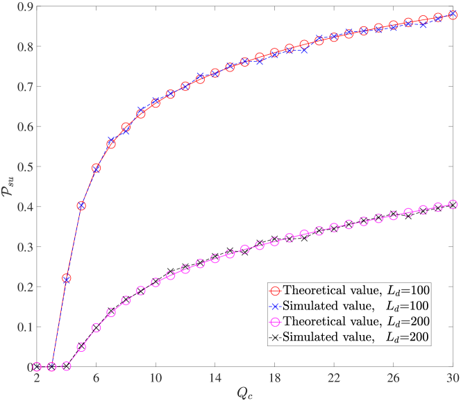
Figure 5: Successful transmission probability $\mathcal{P}_{su}$ vs. design parameter $Q_{c}$ with $P_{max}=20$dBm, $N_{0}=0$dBm.

We count the number of the false alarm and miss detection events as $N_{FA}$ and $N_{MD}$, respectively. Then, the simulated DEP is calculated as

$${\text{Simulated\quad\!\!\!\!}}\xi=100\%\times\frac{N_{FA}+N_{MD}}{10000}.$$ (63)

To validate Theorem 3, we provide plots in Fig. 6 for the simulated and theoretical results of DEP $\xi$ under the CIPC scheme. From Fig. 6, we can see that the simulation results of $\xi$ match well with the corresponding theoretical curves for different maximum transmission power $P_{max}$, indicating that our theoretical performance analysis can be used to model the DEP of the considered system efficiently. Additionally, it is observed that the minimum DEP at $P_{max}=20$dBm is lower than that at $P_{max}=12$dBm. It suggests that a larger $P_{max}$ makes it easier for Willie to detect covert communications in the worst-case scenario.

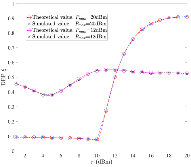
Figure 6: DEP $\xi$ vs. detection threshold $\tau$ with $L_{d}=100$, $Q_{c}=5$, $N_{0}=0$dBm.

IV-B Minimum DEP $\xi^{*}$ Analysis

To validate the effectiveness of the optimal $\tau$ search range provided in Theorem 4, we illustrate Fig. 7 and Fig. 8 under two different maximum transmission power constraints, $P_{max}=12$ dBm and $P_{max}=20$ dBm, respectively. According to Equations (52) and (53), we calculate the corresponding $\tau_{min}$ and $\tau_{max}$, highlighted by black and pink lines, respectively. It is observed that the black and pink lines accurately encompass the interval for $\tau$ corresponding to the minimum DEP. Moreover, in the zoomed-in section of Fig. 7, the minimum value of the DEP lower bound (blue line) differs from the original DEP’s minimum value (red line) by less than $0.02$. Similarly, in the zoomed-in part of Fig. 8, the minimum value of the DEP lower bound (blue line) is virtually identical to the original DEP’s minimum value (red line), significantly less than $0.01$. This demonstrates the rationality of the DEP lower bound provided in Lemma 1.

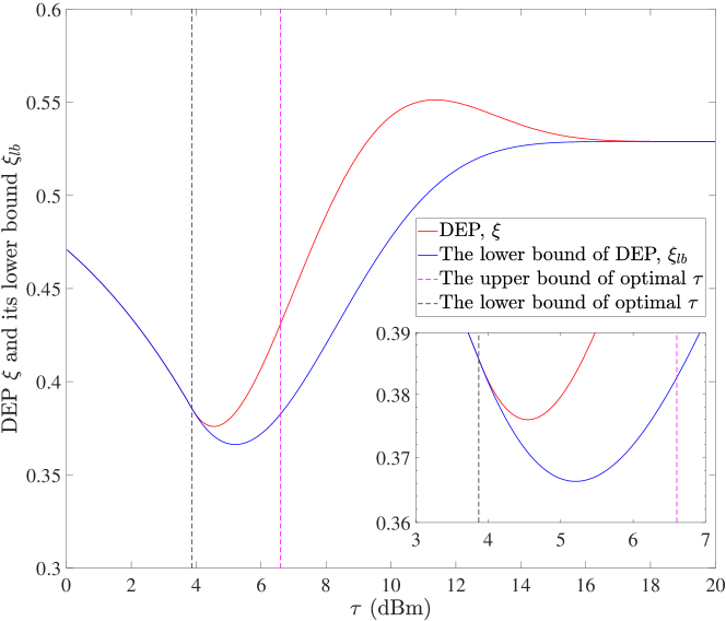
Figure 7: DEP $\xi$ and a lower bound of DEP $\xi_{lb}$ vs. detection threshold $\tau$ with $P_{max}=12$dBm, $L_{d}=100$, $Q_{c}=5$, $N_{0}=0$dBm.

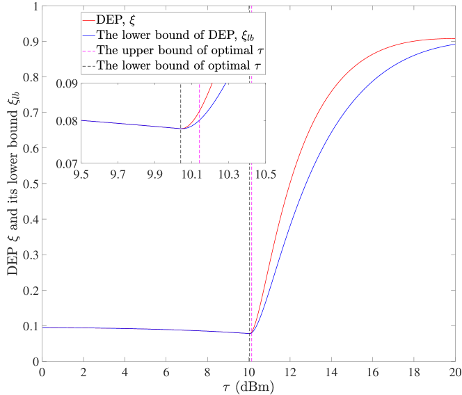
Figure 8: DEP $\xi$ and a lower bound of DEP $\xi_{lb}$ vs. detection threshold $\tau$ with $P_{max}=20$dBm, $L_{d}=100$, $Q_{c}=5$, $N_{0}=0$dBm.

Further, we plot Fig. 9 to explore how the maximum transmit power $P_{max}$ affects the minimum DEP $\xi^{*}$ under the CIPC scheme. From Fig. 9 we can observe that as $P_{max}$ increases, $\xi^{*}$ initially increases from zero, then decreases back to zero. This occurs because when $P_{max}$ is particularly low, covert communication conditions cannot be met, leading the warden to always correctly infer the absence of covert communication; conversely, when $P_{max}$ is significantly high, covert communication is easily exposed, and the warden always correctly infers the presence of covert communication without error. Furthermore, Fig. 9 reveals that, for a fixed $Q_{c}$, larger $L_{d}$ values correspond to higher peaks in $\xi^{*}$. This is attributed to the fact that larger $L_{d}$ results in greater FD, and the deteriorated CSI impacts both the decision on whether to undertake covert transmission and the setting of the covert transmission power, consequently leading to poorer covertness.

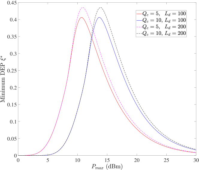
Figure 9: Minimum DEP $\xi^{*}$ vs. the maximum transmit power $P_{max}$ with $N_{0}=0$dBm.

IV-C Optimal CR $\bar{R}_{ab}$ Analysis

To examine the specific influence of $L_{d}$ and $Q_{c}$ on CR $\bar{R}_{ab}$ without/with covertness constraints, two three-dimensional plots, Fig. 10 and Fig. 11, are presented. In Fig. 10, we can observe that as $L_{d}$ increases from zero, $\bar{R}_{ab}$ initially rises rapidly and then decreases slowly. The initial increase in $L_{d}$ provides more data symbol positions for covert communication, enhancing the amount of information. However, further increases in $L_{d}$ lead to more severe FD, adversely affecting CR. In the dimension of $Q_{c}$, $\bar{R}_{ab}$ similarly exhibits a trend of initial increase followed by a decrease. This occurs because as $Q_{c}$ increases, it allocates more resources to covert communication, enhancing the probability of successful transmission, as previously illustrated in Fig. 5. However, further increases in $Q_{c}$ raise the threshold for conducting covert communication, significantly reducing the probability of conducting covert communication. In such cases, even if the probability of successful transmission is $1$, the degradation of CR cannot be avoided.

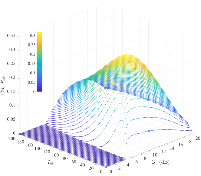
Figure 10: CR $\bar{R}_{ab}$ vs. $Q_{c}$ and $L_{d}$ under $P_{max}=20$dBm and $N_{0}=0$dBm, without covert constraints.

Comparing the planes formed by $L_{d}$ and $Q_{c}$ in Fig. 10 and Fig. 11 it is observable that the latter contains more purple points, indicating a greater number of instances where the CR equals zero. This discrepancy arises because Fig. 11 accounts for the covertness constraint. When the optimization variables fall outside the feasible region, the optimization problem becomes meaningless, and thus, CR is assigned a value of zero.

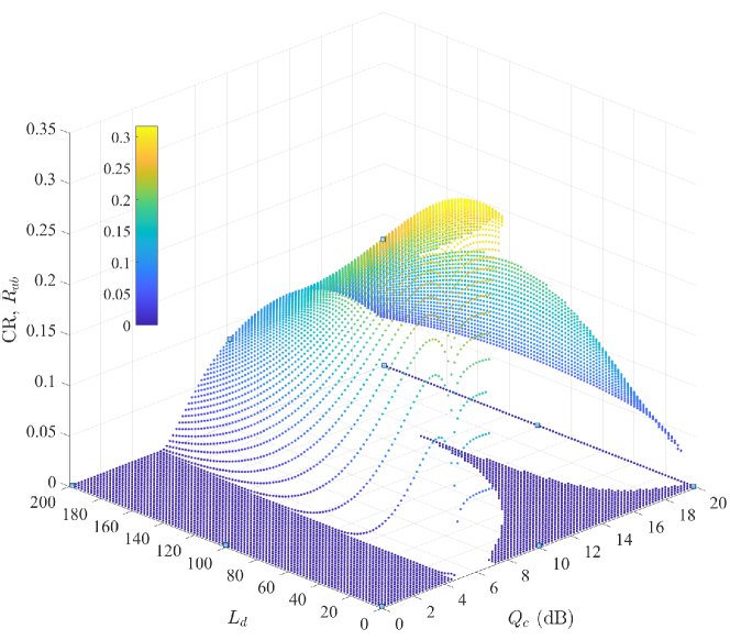
Figure 11: CR $\bar{R}_{ab}$ vs. $P_{max}$ under $P_{max}=20$dBm and $N_{0}=0$dBm, with covert constraints ($\epsilon=0.1$).

To further understand the optimization problem, Fig. 12 illustrates how the maximal CR $\bar{R}_{ab}^{*}$ under covert constraints varies with $P_{max}$. For a given $R_{ab}$ and $N_{0}$, as $P_{max}$ increases, the optimal $\bar{R}_{ab}^{*}$ initially rises quickly and then stabilizes. This phenomenon occurs because an increased $P_{max}$ leads to a higher $Q_{c}$, benefiting the enhancement of $\bar{R}_{ab}^{*}$. However, when $P_{max}$ is sufficiently large, the optimization becomes strictly constrained by $\xi^{*}$, preventing further increases in $\bar{R}_{ab}^{*}$. Additionally, for a fixed $N_{0}$, a smaller predefined transmission rate (i.e., $R_{ab}=1.0$ bits per channel use) results in a higher $\bar{R}_{ab}^{*}$ at a lower $P_{max}$ range. As $P_{max}$ grows, a larger predefined transmission rate (i.e., $R_{ab}=1.5$ bits per channel use) achieves a higher $\bar{R}_{ab}^{*}$. This is attributed to insufficient transmission power coupled with an overly ambitious predefined transmission rate, which raises the transmission outage probability, thus impairing the CR. For a constant $R_{ab}$, lower noise levels favor the $\bar{R}_{ab}^{*}$ since the CEE increases with increasing $N_{0}$. However, when $P_{max}$ is significantly large, the performance gap for different $N_{0}$ narrows to zero.

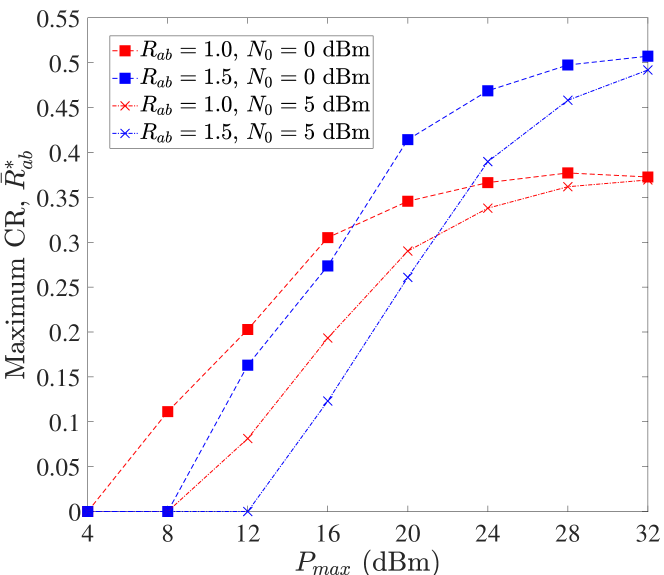
Figure 12: Maximal CR $\bar{R}_{ab}^{*}$ vs. $P_{max}$ with covert constraints ($\epsilon=0.1$).

V CONCLUSIONS

This paper focuses on two-hop relay systems to investigate the combined influence of CEE and FD on covert communication performance within the CIPC framework. We have developed theoretical models that reveal the inherent relationship between imperfect CSI and covert communication metrics such as DEP and CR. Furthermore, we have formulated optimization problem to maximize CR under a covertness constraint, highlighting the profound impact of imperfect CSI on covert communication performance. Our results reveal that careful joint parameter design can mitigate the adverse effects of CEE and FD on covert performance. This study aims to lay the groundwork for future advancements in enhancing covert communication performance in wireless systems challenged by imperfect CSI.

References

- [1] B. A. Bash, D. Goeckel and D. Towsley, “Square root law for communication with low probability of detection on AWGN channels,” in Proc. IEEE Int. Symp. Inf. Theory, Cambridge, MA, USA, Jul. 2012, pp. 448-452.
- [2] X. Chen et al., “Covert communications: A comprehensive survey,” IEEE Commun. Surveys Tuts., vol. 25, no. 2, pp. 1173-1198, 2nd Quart. 2023.
- [3] I. Makhdoom, M. Abolhasan and J. Lipman, “A Comprehensive Survey of Covert Communication Techniques Limitations and Future Challenges,” Comput. Secur., pp. 102784, 2022.
- [4] Y. Jiang, L. Wang, H. Zhao and H.-H. Chen, “Covert communications in D2D underlaying cellular networks with power domain NOMA,” IEEE Syst. J., vol. 14, no. 3, pp. 3717-3728, Sept. 2020.
- [5] L. Tao, W. Yang, S. Yan, D. Wu, X. Guan, D. Chen, “Covert communication in downlink NOMA systems with random transmit power,” IEEE Wirel. Commun. Lett., vol. 9, no. 11, pp. 2000-2004, Nov. 2020.
- [6] Y. Cheng, J. Lu, D. Niyato, B. Lyu, M. Xu and S. Zhu, “Performance analysis of jammer-aided covert RIS-NOMA systems,” in Proc. IEEE Global Commun. Conf. (GLOBECOM), Rio de Janeiro, Brazil, Dec. 2022, pp. 2716-2721.
- [7] L. Lv, Q. Wu, Z. Li, Z. Ding, N. Al-Dhahir and J. Chen, “Covert communication in intelligent reflecting surface-assisted NOMA systems: Design analysis and optimization” IEEE Trans. Wireless Commun., vol. 21, no. 3, pp. 1735-1750, Mar. 2022.
- [8] Y. Su, H. Sun, Z. Zhang, Z. Lian, Z. Xie and Y. Wang, “Covert communication with relay selection,” IEEE Wirel. Commun. Lett., vol. 10, no. 2, pp. 421-425, Feb. 2021.
- [9] C. Gao, B. Yang, X. Jiang, H. Inamura and M. Fukushi, “Covert communication in relay-assisted IoT systems,” IEEE Internet Things J., vol. 8, no. 8, pp. 6313-6323, 15 Apr. 2021.
- [10] C. Gao, B. Yang, D. Zheng, X. Jiang and T. Taleb, “Cooperative Jamming and Relay Selection for Covert Communications in Wireless Relay Systems,” IEEE Trans. Commun., Oct. 2023.
- [11] S.-Y. Wang and M. R. Bloch, “Covert MIMO communications under variational distance constraint,” IEEE Trans. Inf. Forensics Security, vol. 16, pp. 4605-4620, 2021.
- [12] L. Bai, J. Xu and L. Zhou, “Covert communication for spatially sparse mmwave massive MIMO channels,” IEEE Trans. Commun., vol. 71, no. 3, pp. 1615-1630, Mar. 2023.
- [13] J. Hu, S. Yan, X. Zhou, F. Shu and J. Li, “Covert wireless communications with channel inversion power control in Rayleigh fading,” IEEE Trans. Veh. Technol., vol. 68, no. 12, pp. 12135-12149, Dec. 2019.
- [14] Z. Hadzi-Velkov, S. Pejoski and N. Zlatanov, “Achieving near ideal covertness in NOMA systems with channel inversion power control,” IEEE Commun. Lett., vol. 26, no. 11, pp. 2542-2546, Aug. 2022.
- [15] M. Wang, W. Yang, X. Lu, C. Hu, B. Liu and X. Lv, “Channel inversion power control aided covert communications in uplink NOMA systems,” IEEE Wireless Commun. Lett., vol. 11, no. 4, pp. 871-875, Apr. 2022.
- [16] K. Shahzad, X. Zhou and S. Yan, “Covert communication in fading channels under channel uncertainty,” in Proc. IEEE 85th Veh. Technol. Conf., Sydney, NSW, Australia, Jun. 2017, pp. 1-5.
- [17] S. Ma et al., “Robust beamforming design for covert communications,” IEEE Trans. Inf. Forensics Security, vol. 16, pp. 3026–3038, 2021.
- [18] L. Lv, Z. Li, H. Ding, N. Al-Dhahir and J. Chen, “Achieving covert wireless communication with a multi-antenna relay,” IEEE Trans. Inf. Forensics Security, vol. 17, pp. 760-773, 2022.
- [19] J. Wang, W. Tang, Q. Zhu, X. Li, H. Rao and S. Li, “Covert communication with the help of relay and channel uncertainty” IEEE Wireless Commun. Lett., vol. 8, no. 1, pp. 317-320, Feb. 2019.
- [20] Z. Cheng et al., “Covert surveillance via proactive eavesdropping under channel uncertainty,” IEEE Trans. Commun., vol. 69, no. 6, pp. 4024-4037, Jun. 2021.
- [21] K. Shahzad and X. Zhou, “Covert wireless communications under quasi-static fading with channel uncertainty,” IEEE Trans. Inf. Forensics Security, vol. 16, pp. 1104-1116, Oct. 2021.
- [22] J. Bai, J. He, Y. Chen, Y. Shen and X. Jiang, “On covert communication performance with outdated CSI in wireless greedy relay systems,” IEEE Trans. Inf. Forensics Security, vol. 17, pp. 2920-2935, Aug. 2022.
- [23] E. N. Onggosanusi, A. Gatherer, A. G. Dabak and S. Hosur, “Performance analysis of closed-loop transmit diversity in the presence of feedback delay,” IEEE Trans. Commun., vol. 49, no. 9, pp. 1618-1630, Sept. 2001.
- [24] E. Visotsky and U. Madhow, “Space-time transmit precoding with imperfect feedback” IEEE Trans. Inf. Theory, vol. 47, no. 6, pp. 2632-2639, Sept. 2001.
- [25] A. Sheikholeslami, M. Ghaderi, D. Towsley, B. A. Bash, S. Guha and D. Goeckel, “Multi-Hop Routing in Covert Wireless Networks,” IEEE Trans. Wireless Commun., vol. 17, no. 6, pp. 3656-3669, June 2018.
- [26] H. Wang, Y. Zhang, X. Zhang and Z. Li, “Secrecy and covert communications against UAV surveillance via multi-hop networks,” IEEE Trans. Commun., vol. 68, no. 1, pp. 389-401, Jan. 2020.
- [27] H.-S. Im and S.-H. Lee, “Mobility-assisted covert communication over wireless ad hoc networks,” IEEE Trans. Inf. Forensics Security, vol. 16, pp. 1768–1781, 2021.
- [28] D. Song, Z. Yang, G. Pan, S. Wang and J. An, “RIS-Assisted Covert Transmission in Satellite-Terrestrial Communication Systems,” IEEE Internet Things J., vol. 10, no. 22, pp. 19415-19426, 15 Nov.15, 2023.
- [29] K. Shahzad, X. Zhou, S. Yan, J. Hu, F. Shu and J. Li, “Achieving covert wireless communications using a full-duplex receiver,” IEEE Trans. Wireless Commun., vol. 17, no. 12, pp. 8517-8530, Dec. 2018.
- [30] X. Chen et al., “Multi-antenna covert communication via full-duplex jamming against a warden with uncertain locations,” IEEE Trans. Wireless Commun., vol. 20, no. 8, pp. 5467-5480, Aug. 2021.
- [31] Y. Liu, H. Wu, X. Jiang, “Joint selection of FD/HD and AF/DF for covert communication in two-hop relay systems,” Ad Hoc Networks., Vol. 148, pp. 103207, Jun. 2023.
- [32] M. C. Gursoy, “On the capacity and energy efficiency of training-based transmissions over fading channels,” IEEE Trans. Inf. Theory, vol. 55, no. 10, pp. 4543–4567, Oct. 2009.
- [33] B. He and X. Zhou, “Secure on-off transmission design with channel estimation errors” IEEE Trans. Inf. Forensics Security, vol. 8, no. 12, pp. 1923-1936, Dec. 2013.
- [34] A.P. Dawid, “Conditional independence in statistical theory,” J. Roy. Sta. Soc. B, Stat. Methodol., vol. 41, no. 1, pp. 1-15, 1979.
- [35] I. Bronshtein, K. Semendyayev, G. Musiol and H. Mühlig, Handbook of Mathematics, Berlin, Germany:Springer, 2015.
- [36] U. Niesen, D. Shah, and G. W. Wornell, “Adaptive alternating minimization algorithms,” IEEE Trans. Inf. Theory, vol. 55, no. 3, pp. 1423-1429, Mar. 2009.