On the random generation of Butcher trees

Abstract

We provide a probabilistic representation of the solutions of ordinary differential equations (ODEs) by random generation of Butcher trees. This approach complements and simplifies a recent probabilistic representation of ODE solutions, by removing the need to generate random branching times. The random sampling of trees allows one to improve numerical accuracy by Monte Carlo iterations whereas the finite order truncation of Butcher series can have higher time complexity, as shown in examples.

Keywords:  Ordinary differential equations, Runge-Kutta method, Butcher series, random trees, Monte Carlo method.

Mathematics Subject Classification (2020): 65L06, 34A25, 34-04, 05C05, 65C05.

1 Introduction

Butcher series [But63], [But16] are used to represent the solutions of ordinary differential equations (ODEs) by combining rooted tree enumeration with Taylor expansions, see e.g. Chapters 4-6 of [DB02], and [HLW06] and references therein for applications to geometric numerical integration. Given $f:\mathbb{R}^{d}\to\mathbb{R}^{d}$ a smooth function and $t_{0}<T$, consider the $d$-dimensional autonomous ODE problem

$$\begin{cases}\dot{x}(t)=f(x(t)),&t\in(t_{0},T],\vskip 3.0pt plus 1.0pt minus 1.0pt\\ x(t_{0})=x_{0}\in\mathbb{R}^{d}.&\end{cases}$$ (1.1)

If the solution $x(t)$ is sufficiently smooth at $t=t_{0}$, Taylor’s expansion yields

$$x(t)=x_{0}+(t-t_{0})f(x(t_{0}))+\sum_{k=2}^{\infty}\frac{(t-t_{0})^{k}}{k!}\frac{d^{k-1}}{ds^{k-1}}f(x(s))_{\mid s=t_{0}},$$ (1.2)

for small time $t-t_{0}$. We note that in order to calculate the term of order $k\geq 2$ in the above series, the quantity $x(s)$ in $f(x(s))$ can be replaced with its expansion until the order $k-1$, as the $(k-1)$-$th$ derivative $d^{k-1}/ds^{k-1}$ of $(s-t_{0})^{l}$ vanishes at $s=t_{0}$ when $l\geq k$. As a consequence, the expansion (1.2) can be implemented in the following Mathematica code:

⬇

Taylor[f_, t_, x0__, t0_, k_] := (d = Length[x0];

g[x_] := x0 + f[x0]*(x - t0); h = Array[hh, d];

For[j = 2, j <= k, j++, For[i = 1, i <= d, i++,

h[[i]][z_] = g[x][[i]] + (z - t0)^j/j!*D[f[g[s]][[i]], {s, j - 1}] /. {s -> t0};]; v = {};

For[i = 1, i <= d, i++, v = Append[v, h[[i]][x]]]; g[x_] = v];

Return[g[t]])

f[x__] := {f1[x[[1]], x[[2]]], f2[x[[1]], x[[2]]]}

Taylor[f, t, {x1, x2}, 0, 2]

with sample output

$$\left\{\text{x1}+t\text{f1}(\text{x1},\text{x2})+\frac{1}{2}t^{2}\left(\text{f1}^{(0,1)}(\text{x1},\text{x2})\text{f2}(\text{x1},\text{x2})+\text{f1}(\text{x1},\text{x2})\text{f1}^{(1,0)}(\text{x1},\text{x2})\right),\right.$$

$$\left.\ \ \text{x2}+t\text{f2}(\text{x1},\text{x2})+\frac{1}{2}t^{2}\left(\text{f1}(\text{x1},\text{x2})\text{f2}^{(1,0)}(\text{x1},\text{x2})+\text{f2}(\text{x1},\text{x2})\text{f2}^{(0,1)}(\text{x1},\text{x2})\right)\right\}$$

for $k=2$, $d=2$, and $t_{0}=0$. The series (1.2) can be rewritten using the “elementary differentials”

$$f,\ \nabla f(f),\ \nabla^{2}f(f,f),\ \nabla f(\nabla f(f)),\ldots,$$

as the expansion

$$x(t)=x_{0}+(t-t_{0})f(x_{0})+\frac{(t-t_{0})^{2}}{2}\big{(}\nabla f(f)\big{)}(x_{0})+\frac{(t-t_{0})^{3}}{6}\big{(}\nabla^{2}f(f,f)+\nabla f(\nabla f(f))\big{)}(x_{0})+\cdots,$$ (1.3)

which admits a graph-theoretical expression as the summation

$$x(t)=\sum_{\tau}\frac{(t-t_{0})^{|\tau|}}{\tau!\sigma(\tau)}F(\tau)(x_{0}),$$ (1.4)

over rooted trees $\tau$, where $F(\tau)$ represents elementary differentials, and $\sigma(\tau)$, $\tau!$ respectively represent the symmetry and factorial of the tree $\tau$, see Section 2 for precise definitions.

The series (1.4) can be used to estimate ODE solutions by expanding $x(t)$ into a sum over trees up to a finite order. However, the generation of high order trees is computationally expensive.

We consider the numerical estimation of the series (1.4) using Monte Carlo generation of random trees. Monte Carlo estimators represent an alternative to the truncation of series, and they allow for estimates by iterations that can be paralleled straightforwardly. From a simulation point of view, this amounts to estimating (1.4) as an expected value, by generating random trees $\mathcal{T}$ having a conditional probability distribution of the form

$$\mathbb{P}(\mathcal{T}=\tau\mid|\mathcal{T}|=n)=\frac{c_{n}}{\tau!\sigma(\tau)}$$ (1.5)

over rooted trees $\tau$ of size $|\tau|=n\geq 0$, and $(c_{n})_{n\geq 0}$ is a sequence of positive numbers.

In [PP22], a probabilistic representation of ODE solutions as the expected value of a functional of random Butcher trees has been proposed under suitable integrability conditions. Although this method generates random Butcher trees having the correct probability distribution (1.5), its implementation requires to generate sequences of random branching times. This is motivated by related constructions extending the use of the Feynman-Kac formula to the numerical estimation of the solutions of fully nonlinear partial differential equations by stochastic branching mechanisms and stochastic cascades [Sko64], [INW69], [McK75], [LS97], [HLOT⁺19], [NPP23]. However, although the use of random branching times is required in order to take into account the continuous-time dynamics generated by a Laplace operator, it is not needed in the framework of ODEs.

In this paper, we present a direct and simpler approach to the random generation of Butcher trees. More precisely, we construct a random tree $\mathcal{T}$ whose size complies with a probability distribution $(p_{n})_{n\geq 0}$ on $\mathbb{N}$, such that the solution of the ODE (1.1) admits the following probabilistic representation:

$$x(t)=\mathbb{E}\left[\frac{(t-t_{0})^{|\mathcal{T}|}F(\mathcal{T})(x_{0})}{(|\mathcal{T}|\vee 1)p_{|\mathcal{T}|}}\right],$$ (1.6)

see Theorem 4.2. The Monte Carlo implementation of (1.6) allows us to estimate $x(t)$ at a given $t>t_{0}$ within a (possibly finite) time interval. A major difference with the expansion (1.4) is that the Monte Carlo method proceeds iteratively by randomly sampling trees of arbitrary orders, therefore avoiding the evaluation of (1.4) at a fixed order. The numerical results presented in Figure 2 show in particular that the Monte Carlo evaluation can be more precise than series truncation at comparable runtimes.

We also extend our approach to semilinear ODEs of the form

$$\begin{cases}\dot{x}(t)=Ax(t)+f(x(t)),&t\in(t_{0},T],\vskip 3.0pt plus 1.0pt minus 1.0pt\\ x(t_{0})=x_{0}\in\mathbb{R}^{d},&\end{cases}$$

where $A$ is a linear operator on $\mathbb{R}^{d}$. Here, tree sizes are generated with the Poisson distribution of mean $t>0$, and the impact of the operator $A$ is taken into account via an independent continuous-time Markov chain with generator $A$. In this case, our approach extends the construction presented in [DMT08] for linear PDEs, by replacing the use of linear chains (or paths) with general random trees in the setting of nonlinear ODEs. This construction can also be seen as a randomization of exponential Butcher series, see [HO10], [LO13].

We proceed as follows. In Section 2 we review the construction of Butcher trees for the representation of ODE solutions. Section 3 reviews and proves additional statements needed for labelled trees. In Section 4 we present the algorithm for the random generation of Butcher trees by the random attachment of vertices, with numerical results. Section 5 deals with semilinear ODEs using Poisson distributed tree sizes and a continuous-time Markov chain. The appendix contains the multidimensional extension of the codes presented in the paper.

2 Butcher trees

In this section we review the construction of Butcher trees for the series representation (1.3) of the solution of the ODE (1.1). A rooted tree $\tau=(V,E,\mathchoice{\mathbin{\vbox{\hbox{\scalebox{0.5}{$\displaystyle\bullet$}}}}}{\mathbin{\vbox{\hbox{\scalebox{0.5}{$\textstyle\bullet$}}}}}{\mathbin{\vbox{\hbox{\scalebox{0.5}{$\scriptstyle\bullet$}}}}}{\mathbin{\vbox{\hbox{\scalebox{0.5}{$\scriptscriptstyle\bullet$}}}}})$ is a nonempty set $V$ of vertices and a set of edges $E$ between some of the pairs of vertices, with a specific vertex called the root and denoted by “$\mathchoice{\mathbin{\vbox{\hbox{\scalebox{0.5}{$\displaystyle\bullet$}}}}}{\mathbin{\vbox{\hbox{\scalebox{0.5}{$\textstyle\bullet$}}}}}{\mathbin{\vbox{\hbox{\scalebox{0.5}{$\scriptstyle\bullet$}}}}}{\mathbin{\vbox{\hbox{\scalebox{0.5}{$\scriptscriptstyle\bullet$}}}}}$”, such that the graph $(V,E)$ is connected with no loops. We denote by “$\emptyset$” and “$\mathchoice{\mathbin{\vbox{\hbox{\scalebox{0.5}{$\displaystyle\bullet$}}}}}{\mathbin{\vbox{\hbox{\scalebox{0.5}{$\textstyle\bullet$}}}}}{\mathbin{\vbox{\hbox{\scalebox{0.5}{$\scriptstyle\bullet$}}}}}{\mathbin{\vbox{\hbox{\scalebox{0.5}{$\scriptscriptstyle\bullet$}}}}}$” the empty tree and the single node tree, respectively. The next definition uses the $B^{+}$ operation, see [But21, pages 44-45], namely if $\tau_{1},\ldots,\tau_{m}$ are trees, then $[\tau_{1},\ldots,\tau_{m}]$ denotes the tree $\tau$ formed by introducing a new vertex, which becomes the root of $\tau$, and $m$ new edges from the root of $\tau$ to each of the roots of $\tau_{i}$, $i=1,2,\ldots,m$. We also use the notation

$$[\tau_{1}^{k_{1}},\ldots,\tau_{n}^{k_{n}}]=[\underbrace{\tau_{1},\ldots,\tau_{1}}_{k_{1}\mbox{ \footnotesize terms}},\ldots,\underbrace{\tau_{n},\ldots,\tau_{n}}_{k_{n}\mbox{ \footnotesize terms}}],\quad k_{1},\ldots,k_{n}\in\mathbb{N}.$$

Definition 2.1.

The set of rooted trees is denoted $\mathbf{T}$, and can be defined as the closure of $\emptyset$ and $\mathchoice{\mathbin{\vbox{\hbox{\scalebox{0.5}{$\displaystyle\bullet$}}}}}{\mathbin{\vbox{\hbox{\scalebox{0.5}{$\textstyle\bullet$}}}}}{\mathbin{\vbox{\hbox{\scalebox{0.5}{$\scriptstyle\bullet$}}}}}{\mathbin{\vbox{\hbox{\scalebox{0.5}{$\scriptscriptstyle\bullet$}}}}}$ under the $B^{+}$ operation, i.e.:

1. $\emptyset\in\mathbf{T}$, $\mathchoice{\mathbin{\vbox{\hbox{\scalebox{0.5}{$\displaystyle\bullet$}}}}}{\mathbin{\vbox{\hbox{\scalebox{0.5}{$\textstyle\bullet$}}}}}{\mathbin{\vbox{\hbox{\scalebox{0.5}{$\scriptstyle\bullet$}}}}}{\mathbin{\vbox{\hbox{\scalebox{0.5}{$\scriptscriptstyle\bullet$}}}}}\in\mathbf{T}$,

2. $[\tau_{1},\ldots,\tau_{m}]\in\mathbf{T}$ if $\tau_{1},\ldots,\tau_{m}\in\mathbf{T}$.

The size (or order) of $\tau\in\mathbf{T}$ is defined as the number of its vertices, and denoted by $|\tau|$. In particular, we have $|\emptyset|=0$ and $|\mathchoice{\mathbin{\vbox{\hbox{\scalebox{0.5}{$\displaystyle\bullet$}}}}}{\mathbin{\vbox{\hbox{\scalebox{0.5}{$\textstyle\bullet$}}}}}{\mathbin{\vbox{\hbox{\scalebox{0.5}{$\scriptstyle\bullet$}}}}}{\mathbin{\vbox{\hbox{\scalebox{0.5}{$\scriptscriptstyle\bullet$}}}}}|=1$. For $n\geq 0$, we denote by $\mathbf{T}_{n}$ the subset of trees of order $n$ in $\mathbf{T}$.

Definition 2.2.

The elementary differential of $f\in\mathcal{C}^{\infty}(\mathbb{R}^{d},\mathbb{R}^{d})$ is the mapping $F:\mathbf{T}\to\mathcal{C}^{\infty}(\mathbb{R}^{d},\mathbb{R}^{d})$ defined recursively by

1. $F(\emptyset)=\textbf{Id}$, $F(\mathchoice{\mathbin{\vbox{\hbox{\scalebox{0.5}{$\displaystyle\bullet$}}}}}{\mathbin{\vbox{\hbox{\scalebox{0.5}{$\textstyle\bullet$}}}}}{\mathbin{\vbox{\hbox{\scalebox{0.5}{$\scriptstyle\bullet$}}}}}{\mathbin{\vbox{\hbox{\scalebox{0.5}{$\scriptscriptstyle\bullet$}}}}})=f$,

2. $F(\tau)=\nabla^{m}f(F(\tau_{1}),\ldots,F(\tau_{m}))$ for $\tau=[\tau_{1},\ldots,\tau_{m}]$.

The pair $(\tau,F(\tau))$ is called a Butcher tree, and the map $F$ can be used to express any of the terms involving $f$ in the series (1.3). Indeed, when $|\tau|=n$, $F(\tau)$ takes the form

$$\prod_{i=1}^{n}\nabla^{m_{i}}f=\nabla^{m_{1}}f(\nabla^{m_{2}}f(\cdots),\ldots,\ldots(\ldots,f)\cdots),$$ (2.1)

for some integer sequence $(m_{i})_{i=1,\ldots,n}$ such that $m_{n}=0$ and $m_{1}+\cdots+m_{n}=n-1$.

Given a tree $\tau\in\mathbf{T}$, the map $F$ provides a way to encode each vertex of $\tau$ using $f$ or its derivatives: each vertex with no descendants is coded by $f$, and the vertices with $m$ descendants are coded by $\nabla^{m}f$, for $m\geq 1$. In order to characterize the coefficients of (1.3), we need two functionals defined on trees.

Definition 2.3.

1. The symmetry $\sigma$ of a tree is defined recursively by

   1. $\sigma(\emptyset)=1$, $\sigma(\mathchoice{\mathbin{\vbox{\hbox{\scalebox{0.5}{$\displaystyle\bullet$}}}}}{\mathbin{\vbox{\hbox{\scalebox{0.5}{$\textstyle\bullet$}}}}}{\mathbin{\vbox{\hbox{\scalebox{0.5}{$\scriptstyle\bullet$}}}}}{\mathbin{\vbox{\hbox{\scalebox{0.5}{$\scriptscriptstyle\bullet$}}}}})=1$,

   2. $\sigma([\tau_{1}^{k_{1}},\ldots,\tau_{m}^{k_{m}}]=\prod_{i=1}^{m}k_{i}!\sigma(\tau_{i})^{k_{i}}$ for $\tau_{1},\ldots,\tau_{m}$ distinct and $k_{1},\ldots,k_{m}\in\mathbb{N}$.

2. The factorial (or density) $\tau!$ of a tree $\tau$ is defined by

   1. $\emptyset!=1$, $\mathchoice{\mathbin{\vbox{\hbox{\scalebox{0.5}{$\displaystyle\bullet$}}}}}{\mathbin{\vbox{\hbox{\scalebox{0.5}{$\textstyle\bullet$}}}}}{\mathbin{\vbox{\hbox{\scalebox{0.5}{$\scriptstyle\bullet$}}}}}{\mathbin{\vbox{\hbox{\scalebox{0.5}{$\scriptscriptstyle\bullet$}}}}}\,!=1$,

   2. $\tau!=|\tau|\prod_{i=1}^{m}\tau_{i}!$ for $\tau=[\tau_{1},\ldots,\tau_{m}]$.

Using the above formalism, we obtain the following result.

Proposition 2.4.

[But21, Definition 3.4B, Theorem 3.5C] The series (1.3) can be rewritten as

$$x(t)=\sum_{\tau\in\mathbf{T}}\frac{(t-t_{0})^{|\tau|}}{\tau!\sigma(\tau)}F(\tau)(x_{0}),\qquad t>t_{0},$$ (2.2)

which is called a Butcher series.

The following Mathematica code implements the calculation of the series (2.2) up to any tree order $n\geq 1$, and prints the corresponding trees.

⬇

B[f_, t_, x0_, t0_, n_] := (If[n == 0, Return[x0],

If[n == 1, Return[x0 + (t - t0)*f[x0]],

sample = x0 + (t - t0)*f[x0]; g = Graph[{1 -> 2}];

g = Graph[g, VertexLabels -> {1 -> D[f[ y], y]}];

g = Graph[g, VertexLabels -> {2 -> f[y]}]; m = 1;

sample = sample + (t - t0)^VertexCount[g]*

Product[ff[[2]] , {ff, List @@@ PropertyValue[g, VertexLabels]}] /. {y -> x0};

list = {g};

While[m <= (n - 2), temp = list; list = {};

Do[l = VertexCount[g];

For[j = 1, j <= l, j++, gg = VertexAdd[g, {l + 1}];

gg = Graph[gg, VertexLabels -> {l + 1 -> f[ y]}];

lab = Sort[List @@@ PropertyValue[gg, VertexLabels]][[j]][[2]];

gg = Graph[gg, VertexLabels -> {j -> D[lab, y]}];

gg = EdgeAdd[gg, j -> l + 1]; Print[gg];

sample = sample + (t - t0)^(l + 1)/(l + 1)!*

Product[ff[[2]] , {ff, List @@@ PropertyValue[gg, VertexLabels]}] /. {y -> x0};

list = Append[list, gg]], {g, temp}]; m = m + 1];

Return[sample]]]);

For example, the command B[f,t,x0,t0,4] produces the output

$$\text{x0}+\text{f}(\text{x0})(\text{t}-\text{t0})+\text{f}(\text{x0})(\text{t}-\text{t0})^{2}\text{f}^{\prime}(\text{x0})$$

$$+\frac{1}{6}\text{f}(\text{x0})^{2}(\text{t}-\text{t0})^{3}\text{f}^{\prime\prime}(\text{x0})+\frac{1}{6}\text{f}(\text{x0})(\text{t}-\text{t0})^{3}\text{f}^{\prime}(\text{x0})^{2}$$

$$+\frac{1}{24}\text{f}(\text{x0})(\text{t}-\text{t0})^{4}\text{f}^{\prime}(\text{x0})^{3}+\frac{1}{24}\text{f}(\text{x0})^{3}\text{f}^{(3)}(\text{x0})(\text{t}-\text{t0})^{4}+\frac{1}{6}\text{f}(\text{x0})^{2}(\text{t}-\text{t0})^{4}\text{f}^{\prime}(\text{x0})\text{f}^{\prime\prime}(\text{x0})$$

and enumerates the trees appearing in the series (2.2).

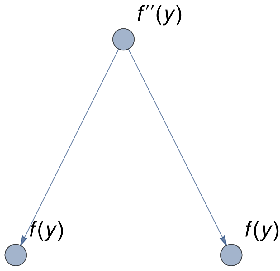
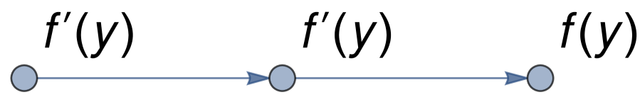
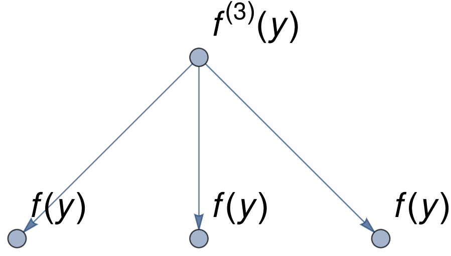
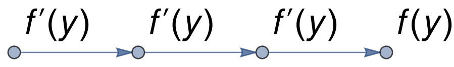
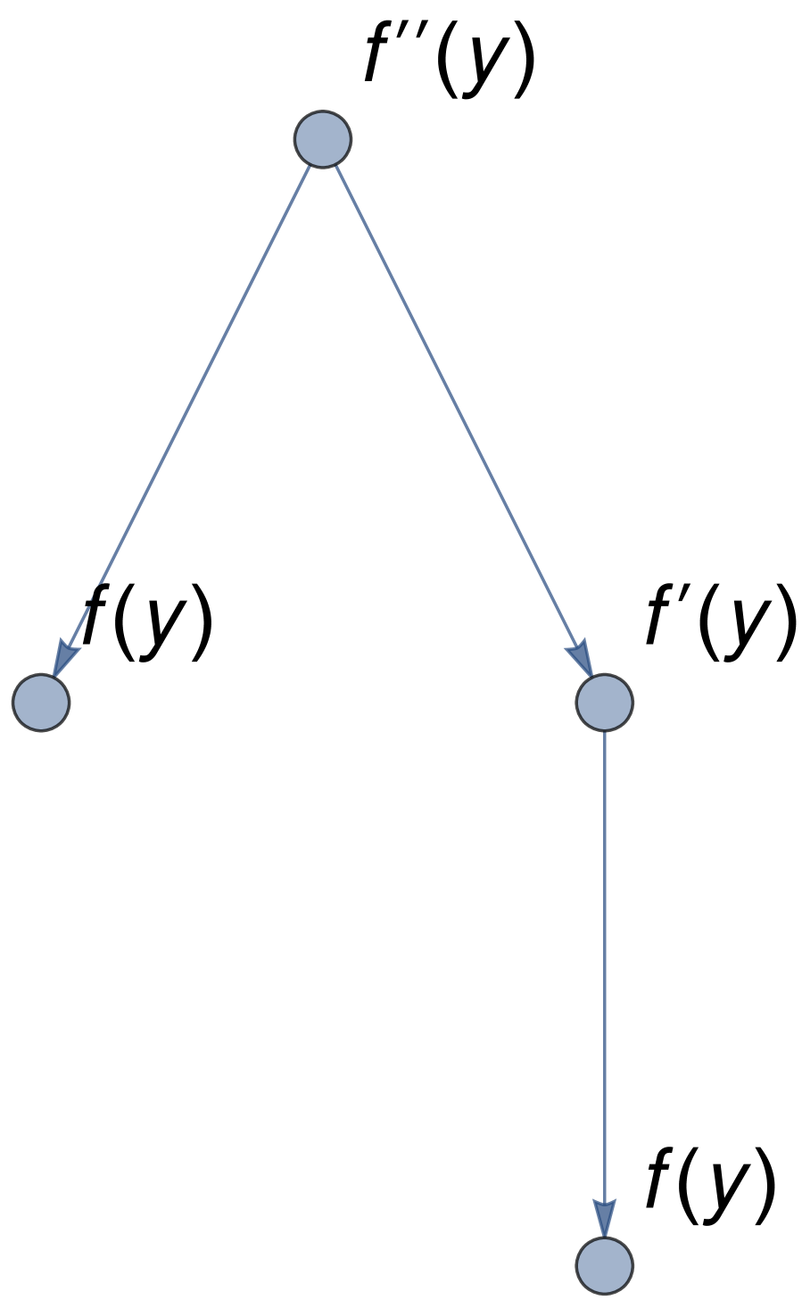
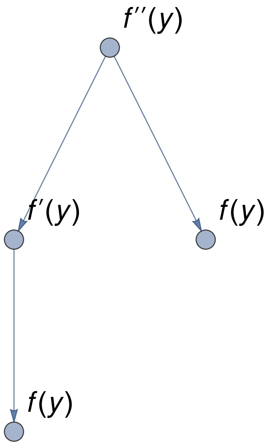
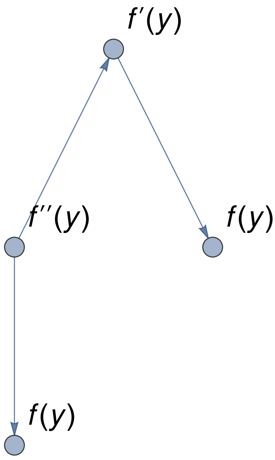
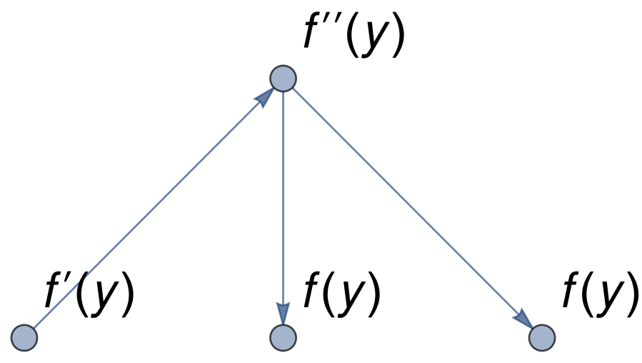
Figure 1: Generation of Butcher trees.

Figure 1 prints directed rooted trees of orders $3$ and $4$, each with a natural orientation away from the root. In addition to the result of Proposition 2.4, the derivatives of the Butcher series (2.2) can be written using the elementary differentials $F$ introduced in Definition 2.2, as follows.

Lemma 2.5.

[But21, Lemma 3.5B] We have

$$x^{(n)}(t)=\sum_{\tau\in\mathbf{T}_{n}}\alpha(\tau)F(\tau)(x(t)),\quad n\geq 1,$$ (2.3)

where

$$\alpha(\tau):=\frac{|\tau|!}{\tau!\sigma(\tau)},\qquad\tau\in\mathbf{T}.$$ (2.4)

Proof.

The proof of (2.3) is conducted by induction using the Faà di Bruno formula [CS96, Theorem 2.1], which states that for a smooth function $g:\mathbb{R}^{d}\to\mathbb{R}^{d^{\prime}}$, the derivatives of $y(t)=g(x(t))$ are given by, for each $n\geq 1$,

$$y^{(n)}(t)=\sum_{k_{1},\ldots,k_{n}\geq 0\atop\sum_{i=1}^{n}ik_{i}=n}\frac{n!}{\prod_{i=1}^{n}k_{i}!(i!)^{k_{i}}}\nabla^{k_{1}+\cdots+k_{n}}g(x(t))\Big{(}\underbrace{\dot{x}(t),\ldots,\dot{x}(t)}_{k_{1}\mbox{ \footnotesize terms}},\ldots,\underbrace{x^{(n)}(t),\ldots,x^{(n)}(t)}_{k_{n}\mbox{ \footnotesize terms}}\Big{)},$$ (2.5)

where the summation is taken over all different nonnegative solutions $(k_{1},\ldots,k_{n})$ of the linear Diophantine equation $\sum_{i=1}^{n}ik_{i}=n$. Now we prove (2.3). We start with $n=1$, for which the result holds. Assume that the result is true for lower orders than $n$. Then we apply Faà di Bruno’s formula (2.5) to derive

$$x^{(n)}(t)=[f(x)]^{(n-1)}(t)$$

$$=\sum_{k_{1},\ldots,k_{n-1}\geq 0\atop\sum_{i=1}^{n-1}ik_{i}=n}\frac{(n-1)!}{\prod_{i=1}^{n-1}k_{i}!(i!)^{k_{i}}}\sum_{\tau_{i}}\prod_{i=1}^{n-1}\left(\frac{i!}{\tau_{i}!\sigma(\tau_{i})}\right)^{k_{i}}\nabla^{k_{1}+\cdots+k_{n-1}}f\left(F(\tau_{1})^{k_{1}},\ldots,F(\tau_{n-1})^{k_{n-1}}\right)(x(t))$$

$$=\sum_{k_{1},\ldots,k_{n-1}\geq 0\atop\sum_{i=1}^{n-1}ik_{i}=n}\frac{n!}{[n\prod_{i=1}^{n-1}(\tau_{i}!)^{k_{i}}][\prod_{i=1}^{n-1}k_{i}!\sigma(\tau_{i})^{k_{i}}]}\nabla^{k_{1}+\cdots+k_{n-1}}f\left(F(\tau_{1})^{k_{1}},\ldots,F(\tau_{n-1})^{k_{n-1}}\right)(x(t))$$

$$=\sum_{\tau\in\mathbf{T}_{n}}\frac{n!}{\tau!\sigma(\tau)}F(\tau)(x(t)),$$

where in the first line, the first summation is taken over all nonnegative integers $(k_{i})_{i=1,\ldots,n-1}$ satisfying $\sum_{i=1}^{n-1}ik_{i}=n-1$, the second summation is taken over all trees $(\tau_{i})_{i=1,\ldots,n-1}$ with $|\tau_{i}|=i$; in the last line $\tau=[\tau_{1}^{k_{1}},\ldots,\tau_{n-1}^{k_{n-1}}]$ so that $|\tau|=1+\sum_{i=1}^{n-1}ik_{i}=n$. ∎

We can also get a tree expansion for $g(x(t))$ with $g\in\mathcal{C}^{\infty}(\mathbb{R}^{d},\mathbb{R}^{d^{\prime}})$. For this purpose, we define the elementary differential $F_{g}$ of $g$ with respect to $f$ using the mapping $F_{g}:\mathbf{T}\to\mathcal{C}^{\infty}(\mathbb{R}^{d},\mathbb{R}^{d})$ given by

$$F_{g}(\emptyset):=\textbf{Id},\ \ F_{g}(\mathchoice{\mathbin{\vbox{\hbox{\scalebox{0.5}{$\displaystyle\bullet$}}}}}{\mathbin{\vbox{\hbox{\scalebox{0.5}{$\textstyle\bullet$}}}}}{\mathbin{\vbox{\hbox{\scalebox{0.5}{$\scriptstyle\bullet$}}}}}{\mathbin{\vbox{\hbox{\scalebox{0.5}{$\scriptscriptstyle\bullet$}}}}}):=g,\ \ \mbox{and}\ \ F_{g}(\tau):=\nabla^{m}g(F(\tau_{1}),\ldots,F(\tau_{m})),\quad\tau=[\tau_{1},\ldots,\tau_{m}].$$ (2.6)

Lemma 2.6.

Let $g\in\mathcal{C}^{\infty}(\mathbb{R}^{d},\mathbb{R}^{d^{\prime}})$. We have

$$g(x(t))=\sum_{\tau\in\mathbf{T}\setminus\{\emptyset\}}\frac{(t-t_{0})^{|\tau|-1}}{(|\tau|-1)!}\alpha(\tau)F_{g}(\tau)(x_{0}).$$ (2.7)

Proof.

By (2.2) and Definition 2.3, we have

$$\begin{split}g(x(t))&=\sum_{m=0}^{\infty}\frac{1}{m!}\nabla^{m}g(x_{0})\left((x(t)-x_{0})^{\otimes m}\right)\\ &=\sum_{m=0}^{\infty}\frac{1}{m!}\sum_{\tau_{1},\ldots\tau_{m}\in\mathbf{T}\setminus\{\emptyset\}}\frac{(t-t_{0})^{\left|\tau_{1}\right|+\ldots+\left|\tau_{m}\right|}}{\prod_{i=1}^{m}\tau_{i}!\sigma(\tau_{i})}\nabla^{m}g\left(F\left(\tau_{1}\right),\ldots,F\left(\tau_{m}\right)\right)(x_{0})\\ &=\sum_{m=0}^{\infty}\sum_{\tau_{1},\ldots\tau_{m}\in\mathbf{T}\setminus\{\emptyset\}}\frac{|\tau|\prod_{j}k_{j}!}{m!}\frac{(t-t_{0})^{|\tau|-1}}{\tau!\sigma(\tau)}\nabla^{m}g\left(F\left(\tau_{1}\right),\ldots,F\left(\tau_{m}\right)\right)(x_{0}),\end{split}$$

where the indexes $k_{1},k_{2},\ldots$ count equal trees among $\tau_{1},\ldots,\tau_{m}$. From the fact that there are $\binom{m}{k_{1},k_{2},\ldots}$ possibilities for writing the tree $\tau$ in the form $[\tau_{1},\ldots,\tau_{m}]$, it then follows that

$$\begin{split}g(x(t))&=\sum_{\tau\in\mathbf{T}\setminus\{\emptyset\}}\frac{|\tau|(t-t_{0})^{|\tau|-1}}{\tau!\sigma(\tau)}\nabla^{m}g\left(F\left(\tau_{1}\right),\ldots,F\left(\tau_{m}\right)\right)(x_{0})\\ &=\sum_{\tau\in\mathbf{T}\setminus\{\emptyset\}}\frac{(t-t_{0})^{|\tau|-1}}{(|\tau|-1)!}\alpha(\tau)\nabla^{m}g\left(F\left(\tau_{1}\right),\ldots,F\left(\tau_{m}\right)\right)(x_{0}),\end{split}$$

where $\alpha(\tau)$ is defined in (2.4). Then, we get (2.7). ∎

In particular, when $g$ is the function $f$ in ODE (1.1), then $F_{f}=F$ and

$$f(x(t))=\sum_{\tau\in\mathbf{T}\setminus\{\emptyset\}}\frac{(t-t_{0})^{|\tau|-1}}{(|\tau|-1)!}\alpha(\tau)F(\tau)(x_{0}),$$

which in turn proves that the Butcher series (2.2) solves (1.1).

3 Labelled trees

Our random generation of Butcher trees will use labelled trees, which provide a combinatorial interpretation of the coefficients appearing in (2.2). By convention, the empty tree $\emptyset$ is labelled by $0$ and the root of any non-empty tree is labelled by $1$.

Definition 3.1.

[But21, (2.5e)] We denote by $\mathbf{T}^{\sharp}$ the set of labelled rooted trees written as $\tau=(V,E,1)$ with vertex sequence $V=\{1,\ldots,n\}$, $n\geq 1$, such that the label of every vertex is smaller than that of each of its children.

We note that the labelling of a tree $\tau$ is not necessarily unique.

Proposition 3.2.

[But21, Theorem 2.5F] The number of all possible labellings of a rooted tree $\tau=(V,E,\mathchoice{\mathbin{\vbox{\hbox{\scalebox{0.5}{$\displaystyle\bullet$}}}}}{\mathbin{\vbox{\hbox{\scalebox{0.5}{$\textstyle\bullet$}}}}}{\mathbin{\vbox{\hbox{\scalebox{0.5}{$\scriptstyle\bullet$}}}}}{\mathbin{\vbox{\hbox{\scalebox{0.5}{$\scriptscriptstyle\bullet$}}}}})$ is given by the coefficient $\alpha(\tau)$ defined in (2.4).

As a consequence of Proposition 3.2, since the labelling of a tree does not affect its elementary differential, we can rewrite (2.2) and (2.3) respectively as

$$x(t)=\sum_{\tau\in\mathbf{T}^{\sharp}}\frac{(t-t_{0})^{|\tau|}}{|\tau|!}F(\tau)(x_{0})\quad\mbox{and}\quad x^{(n)}(t)=\sum_{\tau\in\mathbf{T}^{\sharp}_{n}}F(\tau)(x(t)),\quad n\geq 1,$$ (3.1)

where $\mathbf{T}^{\sharp}_{n}$ denotes the set of labelled trees of order $n\geq 1$, see also [HrW93, Theorem 2.6]. Next, we define a new product on labelled trees that generalizes the beta-product, see [But21, Section 2.1], cf. also § 1.5 of [CL01].

Definition 3.3 (Grafting product).

Let $\tau_{1}=(V_{1},E_{1},1)$ and $\tau_{2}=(V_{2},E_{2},1)$ be two labelled trees, and let $l\in V_{1}=\{1,\ldots,|\tau_{1}|\}$.

• The grafting product with label $l$ of $\tau_{1}$ and $\tau_{2}$, denoted by $\tau_{1}*_{l}\tau_{2}$, is the tree of order $|\tau_{1}|+|\tau_{2}|$ formed by grafting (attaching) $\tau_{2}$ from its root to the vertex $l$ of $\tau_{1}$, so that the vertices of $\tau_{2}$ become descendants of the vertex $l$.

• The tree $\tau_{1}*_{l}\tau_{2}$ is labelled by keeping the labels of $\tau_{1}$, and by adding $|\tau_{1}|$ to the labels of $\tau_{2}$.

For any labelled tree $\tau$, we let $\emptyset*_{0}\tau=\tau*_{l}\emptyset=\tau$ for all $0\leq l\leq|\tau|$, and keep the labels of $\tau$.

Remark 3.4.

1. The beta-product is a grafting product with label $1$, as the second tree is always attached to the root of the first one.

2. The $B^{+}$ operation can also be expressed by grafting-products, by forgetting labelling. For example, we have $[\tau_{1},\tau_{2}]=\mathchoice{\mathbin{\vbox{\hbox{\scalebox{0.5}{$\displaystyle\bullet$}}}}}{\mathbin{\vbox{\hbox{\scalebox{0.5}{$\textstyle\bullet$}}}}}{\mathbin{\vbox{\hbox{\scalebox{0.5}{$\scriptstyle\bullet$}}}}}{\mathbin{\vbox{\hbox{\scalebox{0.5}{$\scriptscriptstyle\bullet$}}}}}*_{1}\tau_{1}*_{1}\tau_{2}=\mathchoice{\mathbin{\vbox{\hbox{\scalebox{0.5}{$\displaystyle\bullet$}}}}}{\mathbin{\vbox{\hbox{\scalebox{0.5}{$\textstyle\bullet$}}}}}{\mathbin{\vbox{\hbox{\scalebox{0.5}{$\scriptstyle\bullet$}}}}}{\mathbin{\vbox{\hbox{\scalebox{0.5}{$\scriptscriptstyle\bullet$}}}}}*_{1}\tau_{2}*_{1}\tau_{1}$.

We note that any labelling is equivalent to a sequence of grafting of dots. In the next lemma we let $\triangle_{0}:=\{0\}$, and

$$\triangle_{n}:=\{(l_{1},\ldots,l_{n})\ :\ 1\leq l_{i}\leq i,\ i=1,\ldots,n\},\quad n\geq 1.$$

Lemma 3.5.

1. Given $\tau$ a labelled tree with $|\tau|\geq 2$, there is a unique sequence $(l_{i})_{1\leq i\leq|\tau|-1}$ in $\triangle_{|\tau|-1}$ such that

   $$\tau=\mathchoice{\mathbin{\vbox{\hbox{\scalebox{0.5}{$\displaystyle\bullet$}}}}}{\mathbin{\vbox{\hbox{\scalebox{0.5}{$\textstyle\bullet$}}}}}{\mathbin{\vbox{\hbox{\scalebox{0.5}{$\scriptstyle\bullet$}}}}}{\mathbin{\vbox{\hbox{\scalebox{0.5}{$\scriptscriptstyle\bullet$}}}}}*_{l_{1}}\mathchoice{\mathbin{\vbox{\hbox{\scalebox{0.5}{$\displaystyle\bullet$}}}}}{\mathbin{\vbox{\hbox{\scalebox{0.5}{$\textstyle\bullet$}}}}}{\mathbin{\vbox{\hbox{\scalebox{0.5}{$\scriptstyle\bullet$}}}}}{\mathbin{\vbox{\hbox{\scalebox{0.5}{$\scriptscriptstyle\bullet$}}}}}*_{l_{2}}\cdots*_{l_{|\tau|-1}}\mathchoice{\mathbin{\vbox{\hbox{\scalebox{0.5}{$\displaystyle\bullet$}}}}}{\mathbin{\vbox{\hbox{\scalebox{0.5}{$\textstyle\bullet$}}}}}{\mathbin{\vbox{\hbox{\scalebox{0.5}{$\scriptstyle\bullet$}}}}}{\mathbin{\vbox{\hbox{\scalebox{0.5}{$\scriptscriptstyle\bullet$}}}}}.$$ (3.2)

2. For any $n\geq 2$, the map which sends $\tau\in\mathbf{T}^{\sharp}_{n}$ to the sequence $(l_{1},\ldots,l_{n-1})$ determined by (3.2) is a bijection from $\mathbf{T}^{\sharp}_{n}$ to $\triangle_{n-1}$.

Proof.

We prove $(i)$ by induction on $|\tau|$. The case $|\tau|=2$ is verified since $\tau=\mathchoice{\mathbin{\vbox{\hbox{\scalebox{0.5}{$\displaystyle\bullet$}}}}}{\mathbin{\vbox{\hbox{\scalebox{0.5}{$\textstyle\bullet$}}}}}{\mathbin{\vbox{\hbox{\scalebox{0.5}{$\scriptstyle\bullet$}}}}}{\mathbin{\vbox{\hbox{\scalebox{0.5}{$\scriptscriptstyle\bullet$}}}}}*_{1}\mathchoice{\mathbin{\vbox{\hbox{\scalebox{0.5}{$\displaystyle\bullet$}}}}}{\mathbin{\vbox{\hbox{\scalebox{0.5}{$\textstyle\bullet$}}}}}{\mathbin{\vbox{\hbox{\scalebox{0.5}{$\scriptstyle\bullet$}}}}}{\mathbin{\vbox{\hbox{\scalebox{0.5}{$\scriptscriptstyle\bullet$}}}}}$. Suppose that (3.2) holds for all trees $\tau$ such that $|\tau|=n$, and let $\tau$ be a labelled tree with $|\tau|=n+1$. Denote by $\tau_{-}$ the subtree obtained by removing the vertex with label $n+1$ from $\tau$. It is clear from Definition 3.1 that the parent of the vertex $n+1$ has label $l$ not bigger than $n$, hence $\tau=\tau_{-}*_{l}\mathchoice{\mathbin{\vbox{\hbox{\scalebox{0.5}{$\displaystyle\bullet$}}}}}{\mathbin{\vbox{\hbox{\scalebox{0.5}{$\textstyle\bullet$}}}}}{\mathbin{\vbox{\hbox{\scalebox{0.5}{$\scriptstyle\bullet$}}}}}{\mathbin{\vbox{\hbox{\scalebox{0.5}{$\scriptscriptstyle\bullet$}}}}}$ has the form (3.2). The converse of $(i)$ holds, since for each $n\geq 2$, the sequence $(l_{1},\ldots,l_{n-1})\in\triangle_{n-1}$ determines a unique tree $\mathchoice{\mathbin{\vbox{\hbox{\scalebox{0.5}{$\displaystyle\bullet$}}}}}{\mathbin{\vbox{\hbox{\scalebox{0.5}{$\textstyle\bullet$}}}}}{\mathbin{\vbox{\hbox{\scalebox{0.5}{$\scriptstyle\bullet$}}}}}{\mathbin{\vbox{\hbox{\scalebox{0.5}{$\scriptscriptstyle\bullet$}}}}}*_{l_{1}}\mathchoice{\mathbin{\vbox{\hbox{\scalebox{0.5}{$\displaystyle\bullet$}}}}}{\mathbin{\vbox{\hbox{\scalebox{0.5}{$\textstyle\bullet$}}}}}{\mathbin{\vbox{\hbox{\scalebox{0.5}{$\scriptstyle\bullet$}}}}}{\mathbin{\vbox{\hbox{\scalebox{0.5}{$\scriptscriptstyle\bullet$}}}}}*_{l_{2}}\cdots*_{l_{n-1}}\mathchoice{\mathbin{\vbox{\hbox{\scalebox{0.5}{$\displaystyle\bullet$}}}}}{\mathbin{\vbox{\hbox{\scalebox{0.5}{$\textstyle\bullet$}}}}}{\mathbin{\vbox{\hbox{\scalebox{0.5}{$\scriptstyle\bullet$}}}}}{\mathbin{\vbox{\hbox{\scalebox{0.5}{$\scriptscriptstyle\bullet$}}}}}$ in $\mathbf{T}^{\sharp}_{n}$. Assertion $(ii)$ follows from $(i)$. ∎

The next result is a consequence of Lemma 3.5-$(ii)$.

Corollary 3.6.

The number of labelled trees of order $n\geq 1$ is given by

$$|\mathbf{T}^{\sharp}_{n}|=\sum_{\tau\in\mathbf{T}^{\sharp}_{n}}1=\sum_{\tau\in\mathbf{T}_{n}}\alpha(\tau)=(n-1)!.$$

Proof. For completeness, we provide a proof that does not rely on Lemma 3.5-$(ii)$. By (2.3) and (2.4) we have $x^{(n)}(t_{0})=\sum_{\tau\in\mathbf{T}_{n}}\alpha(\tau)F(\tau)(x_{0})$. Taking $f(x):=e^{x}$, $x_{0}:=0$ and $t_{0}:=0$, we have $F(\tau)=f^{n}$ for all $\tau\in\mathbf{T}_{n}$ by (2.1), hence the solution $x(t)=-\log(1-t)$ of (1.1) satisfies $x^{(n)}(0)=\sum_{\tau\in\mathbf{T}_{n}}\alpha(\tau)$, and it remains to note that $x^{(n)}(t)=(n-1)!(1-t)^{-n}$, $n\geq 1$. $\square$

4 Random sampling of Butcher trees

In this section we discuss the representation of solutions to (1.1) by the random generation of Butcher trees. Given $\mathcal{T}$ a $\mathbf{T}^{\sharp}$-valued random tree, we let

$$q^{\sharp}_{n}(\tau):=\mathbb{P}\left(\mathcal{T}=\tau\mid|\mathcal{T}|=n\right),\quad\tau\in\mathbf{T}^{\sharp}_{n},$$

denote the conditional distribution of $\mathcal{T}$ given its size is $n\geq 0$. We note that $\mathcal{T}$ is also $\mathbf{T}$-valued, and its conditional distribution on $\mathbf{T}$ is given by

$$q_{n}(\tau):=\mathbb{P}\left(\mathcal{T}=\tau\mid|\mathcal{T}|=n\right)=\sum_{\tau^{\prime}}q^{\sharp}_{n}(\tau^{\prime}),\quad\tau\in\mathbf{T},\quad n\geq 0,$$ (4.1)

where the summation is taken over the possible labellings $\tau^{\prime}$ of $\tau\in\mathbf{T}$.

Definition 4.1.

Given $n\geq 1$, we generate a random labelled tree $\mathcal{T}$ of order $n$ by uniform attachment, as follows:

1. Start from a root $\mathchoice{\mathbin{\vbox{\hbox{\scalebox{0.5}{$\displaystyle\bullet$}}}}}{\mathbin{\vbox{\hbox{\scalebox{0.5}{$\textstyle\bullet$}}}}}{\mathbin{\vbox{\hbox{\scalebox{0.5}{$\scriptstyle\bullet$}}}}}{\mathbin{\vbox{\hbox{\scalebox{0.5}{$\scriptscriptstyle\bullet$}}}}}$ with the label $1$;

2. Starting from a tree $\tau$ with order $l$, $1\leq l\leq n-1$, attach a new vertex with label $l+1$ to an independently and uniformly chosen vertex of $\tau$, until we reach the given order $n$.

By Lemma 3.5-$(ii)$, the random labelled tree $\mathcal{T}$ generated in Definition 4.1 takes the form

$$\mathcal{T}=\mathchoice{\mathbin{\vbox{\hbox{\scalebox{0.5}{$\displaystyle\bullet$}}}}}{\mathbin{\vbox{\hbox{\scalebox{0.5}{$\textstyle\bullet$}}}}}{\mathbin{\vbox{\hbox{\scalebox{0.5}{$\scriptstyle\bullet$}}}}}{\mathbin{\vbox{\hbox{\scalebox{0.5}{$\scriptscriptstyle\bullet$}}}}}*_{\eta_{1}}\mathchoice{\mathbin{\vbox{\hbox{\scalebox{0.5}{$\displaystyle\bullet$}}}}}{\mathbin{\vbox{\hbox{\scalebox{0.5}{$\textstyle\bullet$}}}}}{\mathbin{\vbox{\hbox{\scalebox{0.5}{$\scriptstyle\bullet$}}}}}{\mathbin{\vbox{\hbox{\scalebox{0.5}{$\scriptscriptstyle\bullet$}}}}}*_{\eta_{2}}\cdots*_{\eta_{n-1}}\mathchoice{\mathbin{\vbox{\hbox{\scalebox{0.5}{$\displaystyle\bullet$}}}}}{\mathbin{\vbox{\hbox{\scalebox{0.5}{$\textstyle\bullet$}}}}}{\mathbin{\vbox{\hbox{\scalebox{0.5}{$\scriptstyle\bullet$}}}}}{\mathbin{\vbox{\hbox{\scalebox{0.5}{$\scriptscriptstyle\bullet$}}}}},$$

where $(\eta_{1},\ldots,\eta_{n-1})$ is a uniform random variable taking values in $\triangle_{n-1}$. Next is the main result of this paper.

Theorem 4.2.

Let $(p_{n})_{n\geq 0}$ be a probability distribution on $\mathbb{N}$ such that $p_{n}>0$, $n\geq 0$, and assume that there exists $C>0$ such that

$$|\nabla^{m}f(x_{0})|\leq C,\qquad m\geq 0.$$ (4.2)

Let $\mathcal{T}$ denote the random labelled tree constructed as in Definition 4.1, with the independent order distribution $\mathbb{P}(|\mathcal{T}|=n)=p_{n}$, $n\geq 0$. Then, the solution of the ODE (1.1) admits the probabilistic expression

$$x(t)=\mathbb{E}\left[\frac{(t-t_{0})^{|\mathcal{T}|}F(\mathcal{T})(x_{0})}{(|\mathcal{T}|\vee 1)p_{|\mathcal{T}|}}\right],\qquad t\in[t_{0},t_{0}+1/C).$$ (4.3)

Proof. It follows from Lemma 3.5-$(ii)$ that given $|\mathcal{T}|=n$, the random tree $\mathcal{T}$ is uniformly distributed in $\mathbf{T}^{\sharp}_{n}$, i.e. we have

$$q^{\sharp}_{n}(\tau)=\mathbb{P}\left(\mathcal{T}=\tau\mid|\mathcal{T}|=n\right)=\frac{1}{|\mathbf{T}^{\sharp}_{n}|}=\frac{1}{((n-1)\vee 0)!},$$

in which case $q^{\sharp}_{n}(\tau)$ is independent of $\tau\in\mathbf{T}^{\sharp}_{n}$, and the conditional probability (4.1) is given by

$$q_{n}(\tau)=\frac{\alpha(\tau)}{((n-1)\vee 0)!},\qquad\tau\in\mathbf{T},$$

Hence, we have

$$\mathbb{E}\left[\frac{(t-t_{0})^{|\mathcal{T}|}F(\mathcal{T})(x_{0})}{(|\mathcal{T}|\vee 1)p_{|\mathcal{T}|}}\right] =\sum_{n=0}^{\infty}\frac{(t-t_{0})^{n}p_{n}}{(n\vee 1)p_{n}}\sum_{\tau\in\mathbf{T}_{n}^{\sharp}}q_{n}^{\sharp}(\tau)\mathbb{E}\left[F(\mathcal{T})(x_{0})\mid|\mathcal{T}|=n,\mathcal{T}=\tau\right]$$ (4.4)

$$=\sum_{\tau\in\mathbf{T}^{\sharp}}\frac{(t-t_{0})^{|\tau|}}{|\tau|!}F(\tau)(x_{0})$$

$$=x(t),$$

by the first equation of (3.1). From the assumption (4.2), we have $|F(\tau)(x_{0})|\leq C^{|\tau|}$ for all $\tau\in\mathbf{T}$ such that $|\tau|\geq 1$. The $q$-$th$ integrability of (4.4), $q\geq 1$, can be implied by the bound

$$\mathbb{E}\left[\left|\frac{(t-t_{0})^{|\mathcal{T}|}F(\mathcal{T})(x_{0})}{(|\mathcal{T}|\vee 1)p_{|\mathcal{T}|}}\right|^{q}\right] \leq \frac{|x_{0}|^{q}}{p_{0}^{q-1}}+\sum_{n=1}^{\infty}\frac{(C(t-t_{0}))^{nq}}{n^{q}p_{n}^{q-1}}\sum_{\tau\in\mathbf{T}^{\sharp}_{n}}q^{\sharp}_{n}(\tau)$$ (4.5)

$$= \frac{|x_{0}|^{q}}{p_{0}^{q-1}}+\sum_{n=1}^{\infty}\frac{(C(t-t_{0}))^{nq}}{n^{q}p_{n}^{q-1}},$$

which is finite for $q=1$, provided that $C(t-t_{0})<1$. $\square$

The random generation of Butcher trees in Theorem 4.2 is implemented in the following Mathematica code:

⬇

MCsample[f_, t_, x0_, dist_] := (n = RandomVariate[dist];

If[n == 0, Return[x0/PDF[dist, 0]],

If[n == 1, Return[t*f[x0]/PDF[dist, 1]], g = Graph[{1 -> 2}];

g = Graph[g, VertexLabels -> {1 -> D[f[ y], y]}];

g = Graph[g, VertexLabels -> {2 -> f[y]}]; m = 1;

While[m <= (n - 2), l = VertexCount[g];

j = RandomVariate[DiscreteUniformDistribution[{1, l}]];

g = VertexAdd[g, {l + 1}];

g = Graph[g, VertexLabels -> {l + 1 -> f[ y]}];

lab = Sort[List @@@ PropertyValue[g, VertexLabels]][[j]][[2]];

g = Graph[g, VertexLabels -> {j -> D[lab, y]}];

g = EdgeAdd[g, j -> l + 1]; m++];

sample = Product[ff[[2]] , {ff,

List @@@ PropertyValue[g, VertexLabels]}] /. {y -> x0};

Return[sample*t^n/PDF[dist, n]/n]]]);

f[y_] := Exp[y]

MCsample[f, t, x0, GeometricDistribution[0.5]]

Examples

1. Let $f(y):=e^{y}$, and consider the equation

   $$\dot{x}(t)=e^{x(t)},\quad x(0)=x_{0},\quad t_{0}=0,$$ (4.6)

   with solution

   $$x(t)=-\log(e^{-x_{0}}-t),\qquad t\in[0,e^{-x_{0}}).$$

   In this case, the moment bound (4.5) is sharp with $C=e^{x_{0}}$.

2. Let $f(t,y):=yt+y^{2}$, and consider the equation

   $$\dot{x}(t)=tx(t)+x^{2}(t),\qquad x(0)=1/2,\quad t_{0}=0,$$ (4.7)

   with solution

   $$x(t)=\frac{e^{t^{2}/2}}{2-\int_{0}^{t}e^{s^{2}/2}ds},$$

   see Eq. (223a) in [But16].

Table 1 shows the growth of computation times of the Butcher series command B[f,t,x0,t0,n] whose complexity can be estimated as $(nd)!$, with $n=1,\ldots,8$. For the purpose of benchmarking, all experiments are using tree generation in Mathematica.

$n$	1	2	3	4	5	6	7	8	MC (Geometric)
Eq. (4.6), $d=1$	0s	0s	0.1s	0.1s	0.4	0.5s	3s	21s	22s (70K samples)
Eq. (4.7), $d=2$	0s	0s	0s	0.2s	1s	13s	222s	$>1$h	164s (10K samples)

Table 1: Computation times in seconds for (2.2) with $x_{0}=1$.

Figure 2 compares the numerical solutions of (4.6) and (4.7) by the Butcher series expansion (2.2) and by the probabilistic representation (4.3). The Monte Carlo estimations of (4.3) use the geometric distribution with respectively $70,000$ and $10,000$ samples, see Table 1, so that their runtimes are comparable to those of the Butcher series estimates. The solution of (4.6) is estimated using the above codes for one-dimensional ODEs, and the solution of (4.7) is estimated using the multidimensional codes presented in Appendix A, after rewriting the non-autonomous ODE (4.7) as a two-dimensional autonomous system.

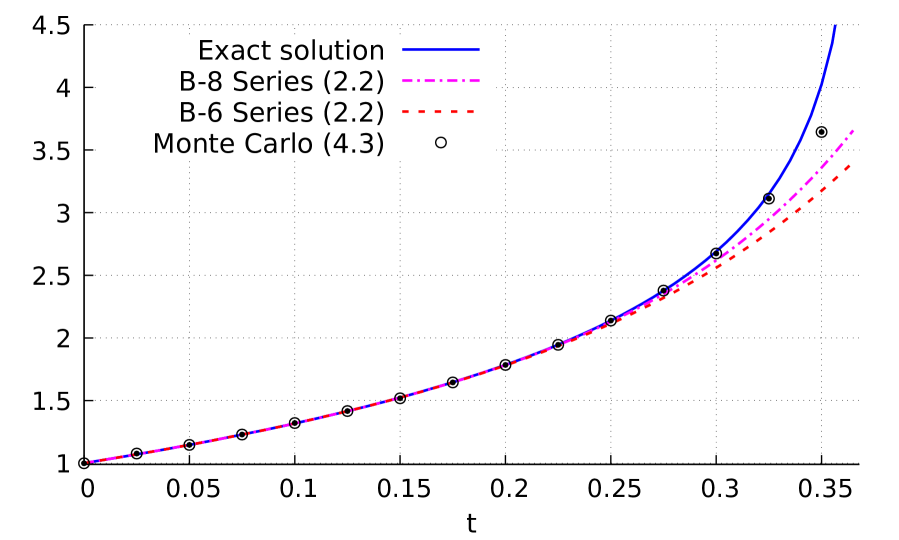
(a) Numerical solutions of (4.6).

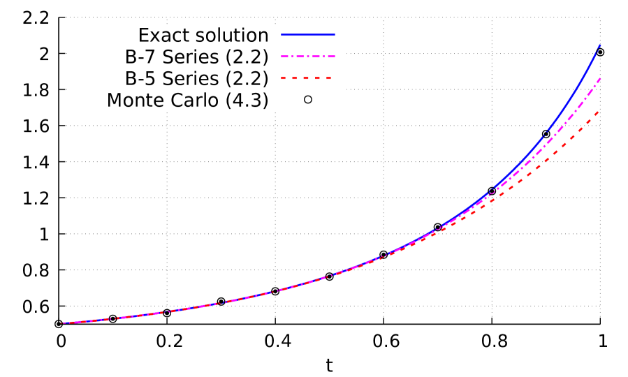
(b) Numerical solutions of (4.7).

Figure 2: Comparisons of (2.2) vs (4.3).

Next, we compare the performance of various probability distributions $(p_{n})_{n\in\mathbb{N}}$ in terms of variance.

Variance analysis

$(i)$ Poisson distribution. Taking $p_{n}:=\lambda^{n}e^{-\lambda}/n!$, $n\geq 0$, to be the Poisson distribution with parameter $\lambda>0$, the variance bound (4.5) is given by the series

$$\frac{x_{0}^{2}}{p_{0}}+\sum_{n=1}^{\infty}\frac{(C(t-t_{0}))^{2n}}{n^{2}p_{n}}=\frac{x_{0}^{2}}{p}+e^{\lambda}\sum_{n=1}^{\infty}\left(\frac{C^{2}(t-t_{0})}{\lambda}\right)^{n}\frac{(n-1)!}{n},$$

which diverges for all $t>t_{0}$.
$(ii)$ Geometric distribution. Taking $p_{n}:=(1-p)p^{n}$, $n\geq 0$, to be the geometric distribution with success probability $1-p$ for some $p\in[0,1)$, the variance bound (4.5) is given by the series

$$\frac{x_{0}^{2}}{p_{0}}+\sum_{n=1}^{\infty}\frac{(C(t-t_{0}))^{2n}}{n^{2}p_{n}}=\frac{x_{0}^{2}}{1-p}+\frac{1}{1-p}\sum_{n=1}^{\infty}\frac{(C^{2}(t-t_{0})^{2}/p)^{n}}{n^{2}},\quad t\in[t_{0},t_{0}+\sqrt{p}/C),$$

in which case the variance is finite.
$(iii)$ Optimal distribution. Using the Lagrangian

$$\frac{x_{0}^{2}}{p_{0}}+\sum_{n=1}^{\infty}\frac{(Ct)^{2n}}{n^{2}p_{n}}+\zeta\left(1-\sum_{n=0}^{\infty}p_{n}\right)$$

with multiplier $\zeta$, we find that the distribution that minimizes the second moment bound (4.5) has the form

$$p_{0}=c_{0}x_{0},\qquad p_{n}=c_{0}\frac{(Ct)^{n}}{n},\qquad n\geq 1,$$ (4.8)

where $c_{0}=(x_{0}-\log(1-Ct))^{-1}$ is a normalization constant, see Figure 3 in which the moment bound (4.5) is plotted as a function of $C\in[0,\sqrt{p}]$ with $t=1$ for the distribution (4.8) (lower bound) and for the geometric distributions with parameters $p=0.5,0.75$, and $x_{0}=1$.

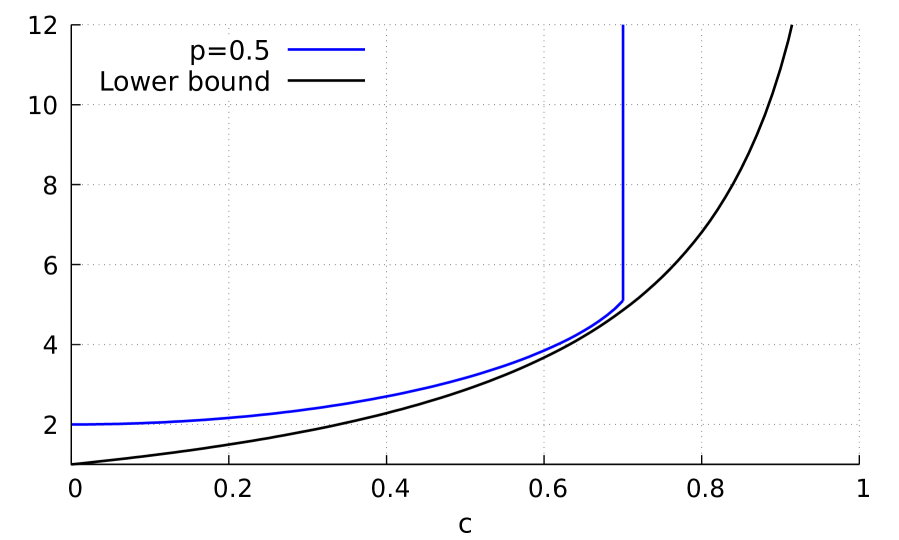
(a) $p=0.5$.

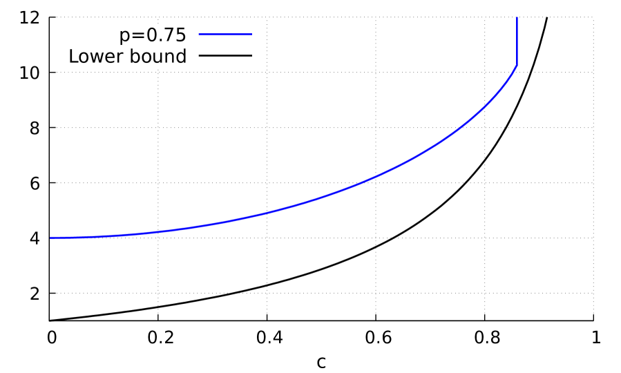
(b) $p=0.75$.

Figure 3: Second moment lower bound.

The graphs of Figure 4 are plotted using the Poisson and geometric distributions with respectively 100,000 and 70,000 Monte Carlo samples, in order to match the 22 seconds computation time of Figure 2-$(a)$ for (4.6), see Table 1.

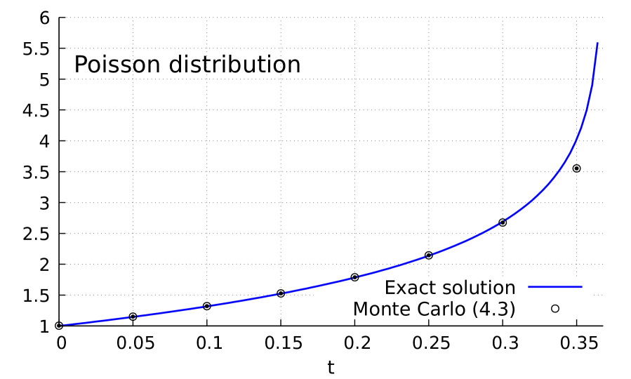
(a) Poisson tree size.

(b) Geometric tree size.

Figure 4: Numerical solution of (4.6) by the Monte Carlo method (4.3).

5 Semilinear case

In this section, we consider the case where the function $f$ in (1.1) involves a linear component, i.e. $f(x)=Ax+g(x)$, where $A$ is a linear operator on $\mathbb{R}^{d}$, in which case the ODE (1.1) becomes

$$\begin{cases}\dot{x}(t)=Ax(t)+g(x(t)),&t\in(t_{0},T],\vskip 3.0pt plus 1.0pt minus 1.0pt\\ x(t_{0})=x_{0}\in\mathbb{R}^{d}.&\end{cases}$$ (5.1)

By the series expansion (2.7) and the variation-of-parameter formulation

$$x(t)=e^{(t-t_{0})A}x_{0}+\int_{t_{0}}^{t}e^{(t-s)A}g(x(s))ds,$$

we have, see [LO13, Theorem 4.5],

$$x(t)=\sum_{\tau\in\mathbf{T}}\alpha(\tau)\phi_{|\tau|}(t,A)F_{g}(\tau)(x_{0}),$$ (5.2)

where $F_{g}$ is defined in (2.6), $\phi_{0}(t,a):=e^{(t-t_{0})a}$, and

$$\phi_{n}(t,a) := \int_{t_{0}}^{t}e^{(t-s)a}\frac{(s-t_{0})^{n-1}}{(n-1)!}ds$$

$$= \int_{t_{0}\leq t_{1}<\cdots<t_{n}\leq t}e^{(t-t_{n})a}dt_{n}\cdots dt_{1},\quad n\geq 1,\ t\geq t_{0},$$

The following proposition follows from the fact that labelling does not change elementary differentials.

Proposition 5.1.

The expansion (5.2) can be rewritten as the exponential B-series

$$x(t)=\sum_{\tau\in\mathbf{T}^{\sharp}}\phi_{|\tau|}(t,A)F_{g}(\tau)(x_{0}).$$ (5.4)

In Theorem 5.2 we propose a canonical way to evaluate the solution to the semilinear equation (5.1) as an expected value over random trees. This can be regarded as a randomization of the exponential Butcher series (5.2) of [LO13], and as a nonlinear extension of the probabilistic representation of [DMT08] which uses linear chains for linear PDEs. In the special case $A=0$, this probabilistic representation recovers (4.3) by generating tree sizes via the Poisson distribution $(p_{n})_{n\geq 0}$ with parameter $t-t_{0}$. Let $(N_{t})_{t\geq t_{0}}$ denote a standard Poisson process with

$$\mathbb{P}(N_{t}=n)=e^{-(t-t_{0})}\frac{(t-t_{0})^{n}}{n!},\quad t\geq t_{0},\ n\geq 0,$$

and increasing sequence of jump times $(T_{i})_{i\geq 1}$, and let $T_{0}=t_{0}$.

Theorem 5.2.

Assume that there exists $C>0$ such that

$$|\nabla^{m}f(x_{0})|\leq C\quad\mbox{and}\quad|\nabla^{m}g(x_{0})|\leq C,\qquad m\geq 0.$$ (5.5)

Let ${\cal T}$ denote the random tree constructed with Poisson random size $N_{t}$ and independent uniform attachment as in Definition 4.1, and let $(X_{t})_{t\geq t_{0}}$ denote an independent continuous-time Markov chain with generator $A$. Then, for $t\in[t_{0},t_{0}+1/C)$ we have

$$x_{i}(t)=e^{(t-t_{0})}\mathbb{E}\big{[}((|\mathcal{T}|-1)\vee 0)!\left(F_{g}(\mathcal{T})(x_{0})\right)_{X_{t-T_{|\mathcal{T}|}}}\ \!\big{|}\ \!X_{t_{0}}=i\big{]},\quad i=1,\ldots,d.$$ (5.6)

Proof. From the fact that the sequence $(T_{i}-T_{i-1})_{i=1,\ldots,n}$ is i.i.d. with common exponential distribution, for any integrable function $h$ on the $n$-dimensional simplex

$$\Delta^{n}_{t}:=\{(t_{1},\ldots,t_{n}):t_{0}\leq t_{1}<\cdots<t_{n}\leq t\},$$

we have

$$\mathbb{E}[\mathbf{1}_{\{N_{t}=n\}}h(T_{1},\ldots,T_{n})]$$

$$=\mathbb{E}\left[\mathbf{1}_{\{t_{0}<T_{n}\leq t<T_{n+1}\}}h\left(T_{1},\ldots,t_{0}+\sum_{i=1}^{n}(T_{i}-T_{i-1})\right)\right]$$

$$=\int_{0<r_{1}+\cdots+r_{n}\leq t-t_{0}}h\left(t_{0}+r_{1},\ldots,t_{0}+\sum_{i=1}^{n}r_{i}\right)e^{-(r_{1}+\cdots+r_{n})}\int_{t-t_{0}-(r_{1}+\cdots+r_{n})}^{\infty}e^{-r_{n+1}}dr_{n+1}dr_{n}\cdots dr_{1}$$

$$=e^{-(t-t_{0})}\int_{0<r_{1}+\cdots+r_{n}\leq t-t_{0}}h\left(t_{0}+r_{1},\ldots,t_{0}+\sum_{i=1}^{n}r_{i}\right)dr_{n}\cdots dr_{1}$$

$$=e^{-(t-t_{0})}\int_{t_{0}\leq t_{1}<\cdots<t_{n}\leq t}h(t_{1},\ldots,t_{n})dt_{n}\cdots dt_{1},$$

where we applied the change of variables $t_{i}=t_{0}+r_{1}+\cdots+r_{i}$ in the last equality. Taking $h(t_{1},\ldots,t_{n}):=e^{(t-t_{n})a}$, $t_{0}\leq t_{1}<\cdots<t_{n}\leq t$, it follows that (5) can be rewritten as

$$\phi_{n}(t,a)=e^{t-t_{0}}\mathbb{E}\left[\mathbf{1}_{\{N_{t}=n\}}e^{(t-T_{n})a}\right],\quad n\geq 0.$$

Next, by construction of the continuous-time Markov chain $(X_{t})_{t\geq t_{0}}$ with generator $A$, we have

$$\left(e^{(t-t_{0})A}x\right)^{i}=\mathbb{E}\left[x_{X_{t}}\ \!\big{|}\ \!X_{t_{0}}=i\right],\quad i=1,\ldots,d,\ x\in\mathbb{R}^{d}.$$

Finally, as the random tree $\mathcal{T}$ is constructed with the Poisson random size $N_{t}$ and independent uniform attachment, we have

$$|\mathcal{T}|=N_{t},\qquad\mathbb{P}\left(\mathcal{T}=\tau\mid|\mathcal{T}|=n\right)=\frac{1}{|\mathbf{T}^{\sharp}_{n}|},\qquad\tau\in\mathbf{T}^{\sharp}_{n}.$$

Combining the above with (5.4), we get

$$x_{i}(t) = e^{t-t_{0}}\sum_{n=0}^{\infty}\sum_{\tau\in\mathbf{T}^{\sharp}_{n}}\mathbb{E}\big{[}\mathbf{1}_{\{N_{t}=n\}}\left(e^{(t-T_{n})A}F_{g}(\tau)(x_{0})\right)^{i}\big{]}$$

$$= e^{t-t_{0}}\sum_{n=0}^{\infty}\sum_{\tau\in\mathbf{T}^{\sharp}_{n}}\mathbb{E}\big{[}\mathbf{1}_{\{N_{t}=n\}}\left(F_{g}(\tau)(x_{0})\right)_{X_{t-T_{n}}}\ \!\big{|}\ \!X_{t_{0}}=i\big{]}$$

$$= e^{t-t_{0}}\sum_{n=0}^{\infty}\sum_{\tau\in\mathbf{T}^{\sharp}_{n}}\mathbb{E}\big{[}\left(F_{g}(\tau)(x_{0})\right)_{X_{t-T_{n}}}\ \!\big{|}\ \!N_{t}=n,X_{t_{0}}=i\big{]}\mathbb{P}(N_{t}=n)$$

$$= e^{t-t_{0}}\sum_{n=0}^{\infty}((n-1)\vee 0)!\mathbb{P}(|\mathcal{T}|=n)$$

$$\qquad\times\sum_{\tau\in\mathbf{T}^{\sharp}_{n}}\mathbb{E}\big{[}\left(F_{g}(\tau)(x_{0})\right)_{X_{t-T_{n}}}\ \!\big{|}\ \!|\mathcal{T}|=n,\mathcal{T}=\tau,X_{t_{0}}=i\big{]}\mathbb{P}\left(\mathcal{T}=\tau\mid|\mathcal{T}|=n\right)$$

$$= e^{t-t_{0}}\mathbb{E}\big{[}((|\mathcal{T}|-1)\vee 0)!\left(F_{g}(\mathcal{T})(x_{0})\right)_{X_{t-T_{|\mathcal{T}|}}}\ \!\big{|}\ \!X_{t_{0}}=i\big{]}.$$

By the definition (2.6) of $F_{g}$ and the bound (5.5), the $q$-$th$ integrability of (5.6), $q\geq 1$, can be controlled by the bound

$$\!\!\!\!\!\!\!\!\!\!\!\!\!\!\!\!\!\!\!\!\!\!\!\!\!\!\mathbb{E}\big{[}\big{|}((|\mathcal{T}|-1)\vee 0)!\left(F_{g}(\mathcal{T})(x_{0})\right)_{X_{t-T_{|\mathcal{T}|}}}\big{|}^{q}\ \!\big{|}\ \!X_{t_{0}}=i\big{]}$$

$$\leq e^{-(t-t_{0})}|x_{0}|^{q}+\mathbb{E}\big{[}\mathbf{1}_{\{|\mathcal{T}|\geq 1\}}\big{|}((|\mathcal{T}|-1)!)^{q}C^{|\mathcal{T}|}\big{|}^{q}\big{]}$$

$$= e^{-(t-t_{0})}|x_{0}|^{q}+e^{-(t-t_{0})}\sum_{n=1}^{\infty}(n-1)!^{q}\frac{C^{nq}}{n!}(t-t_{0})^{n},$$

which is finite for $q=1$, provided that $C(t-t_{0})<1$. $\square$

Appendix A Multidimensional codes

The next Mathematica code estimates the Butcher series (2.2) up to a given order $n\geq 1$ in the multidimensional case. The second component in the output of B[f,t,x0,t0,n] counts the number of trees involved in the Butcher series truncated up to the order $n\geq 1$.

⬇

B[f_, t_, x0__, t0_, n_] := (d = Length[x0];

If[n == 0, Return[{x0, 1}],

If[n == 1, Return[{x0 + (t - t0)*f[x0], 2}], count = 2;

sample = x0 + (t - t0)*f[x0];

g = ConstantArray[Graph[{1 -> 2}], d]; ii = Array[i, n];

For[ii[[1]] = 1, ii[[1]] <= d, ii[[1]]++,

g[[ii[[1]]]] =

Graph[g[[ii[[1]]]],

VertexLabels -> {1 -> D[f[yy], yy[[ii[[1]]]]]}];

g[[ii[[1]]]] =

Graph[g[[ii[[1]]]], VertexLabels -> {2 -> f[yy][[ii[[1]]]]}];

m = 1; count += 1;

sample += (t - t0)^VertexCount[g[[ii[[1]]]]]/2*

Product[ff[[2]] , {ff,

List @@@

PropertyValue[g[[ii[[1]]]], VertexLabels]}] /. {yy ->

x0}]; list = g;

While[m <= (n - 2), temp = list; list = {};

Do[l = VertexCount[g];

For[j = 1, j <= l, j++, gg = VertexAdd[g, {l + 1}];

lab = Sort[List @@@ PropertyValue[gg, VertexLabels]][[j]][[

2]]; For[ii[[l]] = 1, ii[[l]] <= d, ii[[l]]++,

gg = Graph[gg,

VertexLabels -> {l + 1 -> f[ yy][[ii[[l]]]]}];

gg = Graph[gg, VertexLabels -> {j -> D[lab, yy[[ii[[l]]]]]}];

gg = EdgeAdd[gg, j -> l + 1];

GraphPlot[gg,

PlotStyle -> {FontSize -> 20, FontColor -> Red}];

count += 1;

sample += (t - t0)^(l + 1)/(l + 1)!*

Product[ff[[2]] , {ff,

List @@@ PropertyValue[gg, VertexLabels]}] /. {yy ->

x0}; list = Append[list, gg]]], {g, temp}]; m++];

Return[{sample, count}]]]);

x0 = {0, 0.5}; t0 = 0; t1 = 1.3885;

f[y__] := {1, y[[1]]*y[[2]] + y[[2]]^2}

B[f, t, x0, t0, 6]

The next Mathematica code generates a single random Butcher tree sample in (4.3) for a multidimensional ODE.

⬇

MCsample[f_, t_, x0__, t0_, dist_] := (d = Length[x0];

n = RandomVariate[dist];

If[n == 0, Return[x0/PDF[dist, 0]],

If[n == 1, Return[(t - t0)*f[x0]/PDF[dist, 1]],

g = ConstantArray[Graph[{1 -> 2}], d]; ii = Array[i, n];

sample = 0;

For[ii[[1]] = 1, ii[[1]] <= d, ii[[1]]++,

g[[ii[[1]]]] =

Graph[g[[ii[[1]]]],

VertexLabels -> {1 -> D[f[yy], yy[[ii[[1]]]]]}];

g[[ii[[1]]]] =

Graph[g[[ii[[1]]]], VertexLabels -> {2 -> f[yy][[ii[[1]]]]}];

sample += (t - t0)^2/PDF[dist, 2]/2*

Product[ff[[2]] , {ff,

List @@@

PropertyValue[g[[ii[[1]]]], VertexLabels]}] /. {yy ->

x0}]; If[n == 2, Return[sample]]; sample = 0; list = g;

m = 1; While[m <= (n - 2), temp = list; list = {};

Do[l = VertexCount[g];

j = RandomVariate[DiscreteUniformDistribution[{1, l}]];

gg = VertexAdd[g, {l + 1}];

lab = Sort[List @@@ PropertyValue[gg, VertexLabels]][[j]][[2]];

For[ii[[l]] = 1, ii[[l]] <= d, ii[[l]]++,

gg = Graph[gg, VertexLabels -> {l + 1 -> f[ yy][[ii[[l]]]]}];

gg = Graph[gg, VertexLabels -> {j -> D[lab, yy[[ii[[l]]]]]}];

gg = EdgeAdd[gg, j -> l + 1];

GraphPlot[gg,

PlotStyle -> {FontSize -> 20, FontColor -> Red}];

If[m == (n - 2),

sample +=

Product[ff[[2]] , {ff,

List @@@ PropertyValue[gg, VertexLabels]}] /. {yy ->

x0}]; list = Append[list, gg]], {g, temp}]; m++];

Return[sample*(t - t0)^n/PDF[dist, n]/n]]]);

x0 = {0, 0.5}; t0 = 0; t1 = 1.3885;

f[y__] := {1, y[[1]]*y[[2]] + y[[2]]^2}

MCsample[f, t, x0, t0, GeometricDistribution[0.5]]

References

• [But63] J.C. Butcher. Coefficients for the study of Runge-Kutta integration processes. J. Austral. Math. Soc., 3:185–201, 1963.
• [But16] J.C. Butcher. Numerical methods for ordinary differential equations. John Wiley & Sons, Ltd., Chichester, third edition, 2016.
• [But21] J.C. Butcher. B-Series: Algebraic Analysis of Numerical Methods, volume 55 of Springer Series in Computational Mathematics. Springer, Cham, 2021.
• [CL01] F. Chapoton and M. Livernet. Pre-Lie algebras and the rooted trees operad. Internat. Math. Res. Notices, 8:395–408, 2001.
• [CS96] G.M. Constantine and T.H. Savits. A multivariate Faa di Bruno formula with applications. Trans. Amer. Math. Soc., 348(2):503–520, 1996.
• [DB02] P. Deuflhard and F. Bornemann. Scientific Computing with Ordinary Differential Equations, volume 42 of Texts in Applied Mathematics. Springer-Verlag, New York, 2002.
• [DMT08] R.C. Dalang, C. Mueller, and R. Tribe. A Feynman-Kac-type formula for the deterministic and stochastic wave equations and other P.D.E.’s. Trans. Amer. Math. Soc., 360(9):4681–4703, 2008.
• [HLOT+19] P. Henry-Labordère, N. Oudjane, X. Tan, N. Touzi, and X. Warin. Branching diffusion representation of semilinear PDEs and Monte Carlo approximation. Ann. Inst. H. Poincaré Probab. Statist., 55(1):184–210, 2019.
• [HLW06] E. Hairer, C. Lubich, and G. Wanner. Geometric numerical integration, volume 31 of Springer Series in Computational Mathematics. Springer-Verlag, Berlin, second edition, 2006.
• [HO10] M. Hochbruck and A. Ostermann. Exponential integrators. Acta Numer., 19:209–286, 2010.
• [HrW93] E. Hairer, S.P. Nørsett, and G. Wanner. Solving ordinary differential equations. I, volume 8 of Springer Series in Computational Mathematics. Springer-Verlag, Berlin, second edition, 1993. Nonstiff problems.
• [INW69] N. Ikeda, M. Nagasawa, and S. Watanabe. Branching Markov processes I, II, III. J. Math. Kyoto Univ., 8-9:233–278, 365–410, 95–160, 1968-1969.
• [LO13] V.T. Luan and A. Ostermann. Exponential B-series: The stiff case. SIAM Journal on Numerical Analysis, 51(6):3431–3445, 2013.
• [LS97] Y. Le Jan and A. S. Sznitman. Stochastic cascades and $3$-dimensional Navier-Stokes equations. Probab. Theory Related Fields, 109(3):343–366, 1997.
• [McK75] H.P. McKean. Application of Brownian motion to the equation of Kolmogorov-Petrovskii-Piskunov. Comm. Pure Appl. Math., 28(3):323–331, 1975.
• [NPP23] J.Y. Nguwi, G. Penent, and N. Privault. A fully nonlinear Feynman-Kac formula with derivatives of arbitrary orders. Journal of Evolution Equations, 23:Paper No. 22, 29pp., 2023.
• [PP22] G. Penent and N. Privault. Numerical evaluation of ODE solutions by Monte Carlo enumeration of Butcher series. BIT Numerical Mathematics, 62:1921–1944, 2022.
• [Sko64] A.V. Skorokhod. Branching diffusion processes. Teor. Verojatnost. i. Primenen., 9:492–497, 1964.