Thermoelectric transport and current noise through a multilevel Anderson impurity: Three-body Fermi-liquid corrections in quantum dots and magnetic alloys

Abstract

We present a comprehensive Fermi-liquid description for thermoelectric transport and current noise, applicable to multilevel quantum dots (QD) and magnetic alloys (MA) without electron-hole or time-reversal symmetry. Our formulation for the low-energy transport is based on an Anderson model with $N$ discrete impurity levels, and is asymptotically exact at low energies, up to the next-leading order terms in power expansions with respect to temperature $T$ and bias voltage $eV$. The expansion coefficients can be expressed in terms of the Fermi-liquid parameters, which include the three-body correlation functions defined with respect to the equilibrium ground state in addition to the linear susceptibilities and the occupation number $N_{d}$ of impurity electrons. We apply this formulation to SU($N$) symmetric QD and MA, and calculate the correlation functions for $N=4$ and $6$, using numerical renormalization group approach. The three-body correlations are shown to be determined by a single parameter over a wide range of electron fillings $1\lesssim N_{d}\lesssim N-1$ for strong Coulomb interactions $U$, and they also exhibit the plateau structures due to the SU($N$) Kondo effects at integer values of $N_{d}$. We find that the Lorenz number $L=\kappa/(T\sigma)$ for QD and MA, defined as the ratio of the thermal conductivity $\kappa$ to the electrical conductivity $\sigma$, deviates from the universal Wiedemann-Franz value $\pi^{2}/(3e^{2})$ as the temperature increases from $T=0$, showing the $T^{2}$ dependence, the coefficient for which depends on the three-body correlations away from half filling. Furthermore, we find that the current noise for the SU(4) quantum dots and that for SU(6) show a pronounced difference at the quarter $N_{d}/N=1/4$ and $3/4$ fillings. In particular, the linear noise for $N=4$ exhibits a flat peak while the peak for $N=6$ shows a round shape, reflecting the fact that, at these filling points, the SU($N$) Kondo effects occur for $N\equiv 0$ (mod $4$), whereas the intermediate-valence fluctuations occur for $N\equiv 2$ (mod $4$). We also demonstrate the role of three-body correlations on the nonlinear current noise and the other transport coefficients.

I Introduction

The Kondo effect is a fascinating many-body effectKondo (1964); Hewson (1993), taking place in dilute magnetic alloys (MA), quantum dots (QD), and other novel quantum systems such as ultracold atomic gases Ono et al. (2019) and quark matters Yasui and Ozaki (2017). It was shown in 1970’s that the low-energy properties of the Kondo systems can be described by a quantum impurity version of the Fermi-liquid (FL) theory Nozières (1974); Yamada (1975a, b); Shiba (1975); Yoshimori (1976). In particular, using the numerical renormalization group (NRG) approach Wilson (1975); Krishna-murthy et al. (1980a, b), Wilson et al demonstrated that the low-lying excited states of the Kondo and the Anderson models exhibit a one-to-one correspondence with the excitations of the renormalized quasiparticles.

The quasiparticles are asymptotically free in the equilibrium ground state, where the perturbations from the environment or reservoirs, which may depend on external parameters such as frequency $\omega$, temperature $T$, bias voltages $eV$, etc., are absent. As these perturbations are adiabatically switched on, the quasiparticles capture the damping rate of order $\omega^{2}$, $T^{2}$, and $(eV)^{2}$ through the residual interactions between the quasiparticles, and it significantly affects the transport properties Nozières (1974); Yamada (1975a, b); Shiba (1975); Yoshimori (1976); Hershfield et al. (1992); Oguri (2001). When the electron-hole or the time-reversal symmetry is broken by a potential or external fields, the quasiparticles also capture the energy shift of order $\omega^{2}$, $T^{2}$, and $(eV)^{2}$, i.e., the corrections in the same order as the ones due to damping rate. The contributions of these higher-order energy shifts, however, had not been fully understood until very recently.

It has recently been clarified that these higher-order energy shifts of quasiparticles can be described exactly in terms of the three-body correlations between impurity electrons. The proof was given in two different ways, which complement each other. One is given by Mora et al and Filippone et al Mora (2009); Mora et al. (2009, 2015); Filippone et al. (2017), extending Nozières’ descriptionNozières (1974) that is based on an invariance against the “floating of Kondo resonance on the Fermi sea”. The other is based on the higher-order Fermi-liquid relations Oguri and Hewson (2018a, b, c), which can be derived from the Ward identities for the second derivatives of the self-energy, extending Yamada-Yosida’s field-theoretical approach Yamada (1975a, b); Shiba (1975); Yoshimori (1976). These proofs enabled one to express the next-leading order terms of the transport coefficients in terms of three-body correlation functions, and these formulations have been applied to the nonlinear currents, current noise and thermocurrent through quantum impurities without electron-hole or time-reversal symmetry Karki and Kiselev (2017); Karki et al. (2018); Karki and Kiselev (2018); Moca et al. (2018); Teratani et al. (2020a); Oguri et al. (2022); Tsutsumi et al. (2021, 2023).

The purpose of this paper is twofold. The first one is to extend the latest version of the FL theory for treating the thermoelectric transport coefficients of multilevel quantum dots and magnetic alloys, described by the Anderson model with $N$ arbitrary impurity levels. The second one is to demonstrate how the next-leading order terms of various transport coefficients vary with the impurity level $\epsilon_{d}$ and Coulomb interaction $U$. Specifically, for the second purpose, we consider the quantum dots and magnetic alloys having an SU($N$) symmetry, and calculate the three-body correlation functions for $N=4$ and $6$ using the NRG approach. There have been a number of intensive works which theoretically studied low-energy transport: the nonlinear current Glazman and Raikh (1988); Ng and Lee (1988); Hershfield et al. (1992); Wingreen and Meir (1994); Meir and Wingreen (1992); Izumida et al. (1998, 2001); Oguri (2001); Aligia (2012, 2014); Filippone et al. (2018), nonlinear current noise Gogolin and Komnik (2006); Sela et al. (2006); Golub (2006); Sela and Malecki (2009); Mora et al. (2009); Sakano et al. (2011); Karki et al. (2018), and thermoelectric transportCosti et al. (1994); Mora (2009); Costi (2019); Oguri and Hewson (2018c). However, the parameter space for the quantum impurities is so huge that many parts are still left unexplored. In this paper, we explore a whole region of the electron fillings, $0\leq N_{d}\leq N$, in which the occupation number $N_{d}$ of electrons in the impurity levels varies continuously across the various SU($N$) Kondo and the intermediate valence regimes.

One of the advantages of the Kondo systems realized in quantum dots Goldhaber-Gordon et al. (1998a, b); Cronenwett et al. (1998); van der Wiel et al. (2000) is that the information about the many-body quantum states can be probed in such a highly tunable way, for instance, recent experiments have succeeded to directly probe the Kondo screening cloud V. Borzenets et al. (2020). Furthermore, low-energy Fermi-liquid behaviors have experimentally been confirmed for nonequilibrium currents Grobis et al. (2008); Scott et al. (2009), current noiseZarchin et al. (2008); Delattre et al. (2009); Yamauchi et al. (2011); Ferrier et al. (2016); Hata et al. (2021), and themocurrentHsu et al. (2022); Svilans et al. (2018). Internal degrees of freedoms of quantum impurities also bring an interesting variety to the Kondo effect. The systems having the SU($4$) symmetry have been realized, for instance, in the multiorbital semiconductor quantum dots and carbon nanotube (CNT) quantum dots Laird et al. (2015), and have intensively been investigated theoreticallyIzumida et al. (1998); Borda et al. (2003); Choi et al. (2005); Eto (2005); Sakano and Kawakami (2006); Anders et al. (2008); Weymann et al. (2018); Mora (2009); Mora et al. (2009); Filippone et al. (2014); Mantelli et al. (2016); Teratani et al. (2020a, b); Karki and Kiselev (2017) and experimentallySasaki et al. (2000); Jarillo-Herrero et al. (2005); Babić et al. (2004); Makarovski et al. (2007); Cleuziou et al. (2013); Ferrier et al. (2016). Realization of the SU($N$) Kondo effects for various $N>2$ has also been proposed by several authors, using triple quantum dotsKuzmenko et al. (2006); López et al. (2013) and CNTKuzmenko and Avishai (2014). In this paper, we provide a comprehensive FL view of the low-energy transport for SU(4) and SU(6) symmetric QD and MA.

Our results reveal the fact that the three-body correlations exhibit the plateau structures, caused by the SU($N$) Kondo effects occurring at integer fillings $N_{d}=1$, $2$, $\ldots N-1$. We also calculate the Lorenz number $L=\kappa/(T\sigma)$ for QD and MA, defined as the ratio of the thermal conductivity $\kappa$ to the electrical conductivity $\sigma$, and show how it deviates from the universal Wiedemann-Franz value $\pi^{2}/(3e^{2})$ as the temperature increases from $T=0$. Furthermore, we demonstrate that the three-body correlations significantly affect the magnitude of order $T^{2}$ term of $\sigma$, the order $T^{3}$ term of $\kappa$, and the order $|eV|^{3}$ term of nonlinear current and current noise. At quarter $N_{d}/N=1/4$ and three-quarters $3/4$ fillings, the SU($N$) Kondo effects occur for $N\equiv 0$ (mod $4$) while the intermediate valence fluctuations occur for $N\equiv 2$ (mod $4$). We show that this dependence on (mod $4$) causes a pronounced difference appearing in the peak structures of linear noise for $N=4$ and $6$.

This paper is organized as follows. In Sec. II, we describe the multilevel Anderson impurity model for quantum dots and magnetic alloys. Sections III and IV are devoted to the FL descriptions for the next-leading order terms of electrical and thermoelectric transport coefficients for quantum dots, applicable to arbitrary $N$ impurity-level structures. In Sec. V, the low-energy transport formulas for the SU($N$) quantum dots are described in terms of the five FL parameters. We present the NRG results for the three-body correlation functions in Sec. VI. The results for nonlinear current, current noise, and thermoelectric transport through quantum dots are discussed in Secs. VII and VIII. Section IX is devoted to the FL description of the three-body correlations in thermoelectric transport of dilute magnetic alloys. In Sec. X, we discuss the results for the electrical and thermal resistivities of the SU(4) and SU(6) magnetic alloys. Summary is given in Sec. XI. In Appendix, we provide details of the derivations for the transport formulas and additional NRG results for the FL parameters in the SU($N$) cases for $N=2$, $4$, and $6$, for comparison.

II Model

We consider a multi-orbital Anderson impurity coupled to two noninteracting leads on the left ($L$) and right ($R$): $\mathcal{H}=\mathcal{H}_{d}+\mathcal{H}_{c}+\mathcal{H}_{\mathrm{T}}$,

$$\mathcal{H}_{d}= \ \sum_{\sigma=1}^{N}\epsilon_{d\sigma}\,n_{d\sigma}+\frac{1}{2}\sum_{\sigma\neq\sigma^{\prime}}U_{\sigma\sigma^{\prime}}\,n_{d\sigma}n_{d\sigma^{\prime}}\;,$$ (1)

$$\mathcal{H}_{c}= \ \sum_{j=L,R}\sum_{\sigma=1}^{N}\int_{-D}^{D}\!\!d\epsilon\,\epsilon\,c^{\dagger}_{\epsilon j\sigma}c_{\epsilon j\sigma},$$ (2)

$$\mathcal{H}_{\mathrm{T}}= \ -\sum_{j=L,R}\sum_{\sigma=1}^{N}v_{j}\left(\psi_{j,\sigma}^{\dagger}d_{\sigma}+d_{\sigma}^{{\dagger}}\psi_{j,\sigma}\right).$$ (3)

Here, the level index runs over $\sigma=1,2,\ldots,N$. The inter-electron interaction $U_{\sigma\sigma^{\prime}}$ generally depends on $\sigma$ and $\sigma^{\prime}$, with the requirements $U_{\sigma^{\prime}\sigma}=U_{\sigma\sigma^{\prime}}$ for $\sigma^{\prime}\neq\sigma$. For $N=2$, it describes the usual single orbital Anderson model for spin $1/2$ fermions. The operator $d^{{\dagger}}_{\sigma}$ creates an impurity electron with spin $\sigma$ in the impurity level of energy $\epsilon_{d\sigma}$, and $n_{d\sigma}=d^{{\dagger}}_{\sigma}d_{\sigma}$. Conduction electrons in the two lead at $j=L$ and $R$ obey the anti-commutation relation $\{c^{\phantom{\dagger}}_{\epsilon j\sigma},c^{\dagger}_{\epsilon^{\prime}j^{\prime}\sigma^{\prime}}\}=\delta_{jj^{\prime}}\,\delta_{\sigma\sigma^{\prime}}\delta(\epsilon-\epsilon^{\prime})$. The linear combination of the conduction electrons, $\psi_{j,\sigma}\equiv\int_{-D}^{D}d\epsilon\sqrt{\rho_{c}}\,c^{\phantom{\dagger}}_{\epsilon j\sigma}$ with $\rho_{c}=1/(2D)$, couples to the impurity level. The bare level width due to the tunnel couplings is given by $\Delta\equiv\Gamma_{L}+\Gamma_{R}$ with $\Gamma_{j}=\pi\rho_{c}v_{j}^{2}$. We consider the parameter region where the half band-width $D$ is much grater than the other energy scales, $D\gg\max(U_{\sigma\sigma^{\prime}},\Delta,|\epsilon_{d\sigma}|,T,|eV|)$. We use a unit $k_{B}=1$ throughout this paper.

The total number of electrons occupying the impurity levels is given by

$$N_{d}\,\equiv\,\sum_{\sigma=1}^{N}\langle n_{d\sigma}\rangle\,.$$ (4)

The current conservation law, which follows from the Heisenberg equation motion for $n_{d\sigma}$, holds for each component of the occupation number,

$$\frac{\partial n_{d\sigma}}{\partial t}+\widehat{J}_{R,\sigma}-\widehat{J}_{L,\sigma}\,=\,0\,.$$ (5)

Here, $\widehat{J}_{L,\sigma}$ represents the current following from the left lead to the dot, and $\widehat{J}_{R,\sigma}$ the current from the dot to the right lead:

$$\widehat{J}_{L,\sigma}= \ -i\,v_{L}\left(\psi^{\dagger}_{L\sigma}d_{\sigma}-d^{\dagger}_{\sigma}\psi_{L\sigma}\right),$$ (6)

$$\widehat{J}_{R,\sigma}= \ +i\,v_{R}\left(\psi^{\dagger}_{R\sigma}d_{\sigma}-d^{\dagger}_{\sigma}\psi_{R\sigma}\right).$$ (7)

A series of exact relations between the dynamic correlation functions and the static susceptibilities can be derived from the Ward identities, which reflect the current conservation. The Friedel sum rule and the Fermi-liquid relations between the phase shift $\delta_{\sigma}$, the linear susceptibilities $\chi_{\sigma\sigma^{\prime}}$, and the static three-body correlation functions $\chi_{\sigma_{1}\sigma_{2}\sigma_{3}}^{[3]}$ play an essential role in the low-energy Fermi-liquid transport up to next-leading order. The definition of these correlation functions are summarized in Appendix A.

III Fermi-liquid description for nonlinear current noise of QD

We consider the nonequilibrium steady state under a finite bias voltage $eV\equiv\mu_{L}-\mu_{R}$, applied between the two leads by setting the chemical potentials of the left and right leads to be $\mu_{L}$ and $\mu_{R}$, respectively. The retarded Green’s function play a central role in the microscopic description of the Fermi-liquid transport:

$$G_{\sigma}^{r}(\omega)= \ -i\int_{0}^{\infty}dt\,e^{i(\omega+i0^{+})t}\,\Bigl{\langle}\,\Bigl{\{}d_{\sigma}(t),\,d_{\sigma}^{\dagger}\Bigr{\}}\Bigr{\rangle}_{V}\,,$$ (8)

$$A_{\sigma}(\omega)\,\equiv \ -\frac{1}{\pi}\,\mathrm{Im}\,G_{\sigma}^{r}(\omega)\;.$$ (9)

Here, $\langle\cdots\rangle_{V}$ represents a nonequilibrium steady-state average taken with the statistical density matrix, which is constructed at finite bias voltages $eV$ and temperatures $T$, using the Keldysh formalism.Meir and Wingreen (1992); Hershfield et al. (1992); Caroli et al. (1971)

III.1 Differential conductance $dJ/dV$

The nonequilibrium current $J$ through quantum dots can be expressed in terms of the spectral function $A_{\sigma}(\omega)$: Meir and Wingreen (1992); Hershfield et al. (1992)

$$\!\!\!J\,=\,\frac{e}{h}\sum_{\sigma}\int_{-\infty}^{\infty}\!d\omega\,\bigl{[}\,f_{L}(\omega)-f_{R}(\omega)\,\bigr{]}\,\mathcal{T}_{\sigma}(\omega),$$ (10)

$$\!\!\!\mathcal{T}_{\sigma}(\omega)\,=\,\frac{4\Gamma_{L}\Gamma_{R}}{\Gamma_{L}+\Gamma_{R}}\,\pi A_{\sigma}(\omega)\,.$$ (11)

Here, $f_{j}(\omega)\equiv f(\omega-\mu_{j})$ for $j=L$, $R$, with $f(\omega)=[e^{\omega/T}+1]^{-1}$ the Fermi function. Specifically, in this paper, we consider the case where the chemical potentials are applied in a symmetric way:

$$\mu_{L}\,=\,-\mu_{R}\ \equiv\ \frac{1}{2}\,eV\,,$$ (12)

choosing the Fermi level at equilibrium to be the origin of one-particle energies $E_{F}=0$. Note that the role of bias and tunneling asymmetries, $(\mu_{L}+\mu_{R})/2\neq E_{F}$ and $\Gamma_{L}\neq\Gamma_{R}$, has precisely been discussed in Refs. Tsutsumi et al., 2021, 2023.

The nonlinear current $J$ can be expanded in the Fermi liquid regime up to terms of the next-leading order, using the low-energy asymptotic form the spectral function $A_{\sigma}(\omega)$ which has been obtained up to terms of order $\omega^{2}$, $(eV)^{2}$, and $T^{2}$,Oguri et al. (2022) as shown in Eq. (111) in Appendix B. In particular for symmetric junctions with $\Gamma_{L}=\Gamma_{R}$ and $\mu_{L}=-\mu_{R}=eV/2$, the low-energy expansion of the differential conductance takes the form,

$$\frac{dJ}{dV}=\frac{e^{2}}{h}\sum_{\sigma=1}^{N}\left[\,\sin^{2}\delta_{\sigma}-c_{T,\sigma}\left(\pi T\right)^{2}-c_{V,\sigma}\left(eV\right)^{2}\,+\,\cdots\right]$$ (13)

Here, the coefficients $c_{T,\sigma}$ and $c_{T,\sigma}$ of the next leading-order terms can be expressed in terms of the phase shift $\delta_{\sigma}$, the linear susceptibilities $\chi_{\sigma\sigma^{\prime}}$, and the static three-body correlation functions $\chi_{\sigma\sigma^{\prime}\sigma^{\prime\prime}}^{[3]}$, defined in Appendix A:

$$\!\!\!\!c_{T,\sigma}=\frac{\pi^{2}}{3}\Biggl{[}\,-\biggl{(}\chi_{\sigma\sigma}^{2}+2\sum_{\sigma^{\prime}(\neq\sigma)}\chi_{\sigma\sigma^{\prime}}^{2}\biggr{)}\cos 2\delta_{\sigma}$$

$$\qquad\qquad\,+\biggl{(}\chi_{\sigma\sigma\sigma}^{[3]}+\sum_{\sigma^{\prime}(\neq\sigma)}\chi_{\sigma\sigma^{\prime}\sigma^{\prime}}^{[3]}\biggr{)}\frac{\sin 2\delta_{\sigma}}{2\pi}\,\Biggr{]},$$ (14)

$$\!\!\!\!c_{V,\sigma}=\frac{\pi^{2}}{4}\Biggl{[}\,-\biggl{(}\chi_{\sigma\sigma}^{2}+5\sum_{\sigma^{\prime}(\neq\sigma)}\chi_{\sigma\sigma^{\prime}}^{2}\biggr{)}\cos 2\delta_{\sigma}$$

$$\qquad\qquad+\biggl{(}\chi_{\sigma\sigma\sigma}^{[3]}+3\sum_{\sigma^{\prime}(\neq\sigma)}\chi_{\sigma\sigma^{\prime}\sigma^{\prime}}^{[3]}\biggr{)}\frac{\sin 2\delta_{\sigma}}{2\pi}\,\Biggr{]}.$$ (15)

III.2 Nonlinear current noise $S_{\mathrm{noise}}^{\mathrm{QD}}$

We also study the current noise, defined by Hershfield (1992); Teratani et al. (2020a); Oguri et al. (2022)

$$S_{\mathrm{noise}}^{\mathrm{QD}}=\,e^{2}\sum_{\sigma\sigma^{\prime}}\int_{-\infty}^{\infty}\!\!dt\,\left\langle\delta\widehat{J}_{\sigma}(t)\,\delta\widehat{J}_{\sigma^{\prime}}(0)+\delta\widehat{J}_{\sigma^{\prime}}(0)\,\delta\widehat{J}_{\sigma}(t)\right\rangle_{V}.$$ (16)

Here, $\delta\widehat{J}_{\sigma}(t)\equiv\widehat{J}_{\sigma}(t)-\bigl{\langle}\widehat{J}_{\sigma}(0)\bigr{\rangle}_{V}$ represents fluctuations of the symmetrized current:

$$\widehat{J}_{\sigma}\equiv \ \frac{\Gamma_{L}\widehat{J}_{R,\sigma}+\Gamma_{R}\widehat{J}_{L,\sigma}}{\Gamma_{L}+\Gamma_{R}}\;.$$ (17)

Behavior of the current noise in the low-energy Fermi-liquid regime has been studied by several authors, taking into account the three-body correlations Mora et al. (2015, 2009). In the previous work, we have derived the general formula for current noise through the multilevel Anderson impurity model up to terms of order $|eV|^{3}$ for symmetric junctions $\Gamma_{L}=\Gamma_{R}$ and $\mu_{L}=-\mu_{R}=eV/2$ Teratani et al. (2020a); Oguri et al. (2022):

$$S_{\mathrm{noise}}^{\mathrm{QD}}=\frac{2e^{2}}{h}|eV|\sum_{\sigma=1}^{N}\left[\frac{\sin^{2}2\delta_{\sigma}}{4}\,+c_{S,\sigma}\left(eV\right)^{2}+\cdots\right].$$ (18)

The coefficient $c_{S,\sigma}$ for the next-leading order term has been calculated taking into account all components of the Keldysh vertex function together with the asymptotic form of $A_{\sigma}(\omega)$; the result can be expressed in terms of $\delta_{\sigma}$, $\chi_{\sigma\sigma^{\prime}}$, and $\chi_{\sigma\sigma^{\prime}\sigma^{\prime\prime}}^{[3]}$, as

$$\!\!c_{S,\sigma}= \ \frac{\pi^{2}}{12}\Biggl{[}\,\cos 4\delta_{\sigma}\,\chi_{\sigma\sigma}^{2}+\bigl{(}2+3\cos 4\delta_{\sigma}\bigr{)}\sum_{\sigma^{\prime}(\neq\sigma)}\chi_{\sigma\sigma^{\prime}}^{2}$$

$$\quad\ \ +\,4\sum_{\sigma^{\prime}(\neq\sigma)}\cos 2\delta_{\sigma}\cos 2\delta_{\sigma^{\prime}}\,\chi_{\sigma\sigma^{\prime}}^{2}$$

$$\quad\ \ +\,3\sum_{\sigma^{\prime}(\neq\sigma)}\sum_{\sigma^{\prime\prime}(\neq\sigma,\sigma^{\prime})}\sin 2\delta_{\sigma}\,\sin 2\delta_{\sigma^{\prime}}\chi_{\sigma\sigma^{\prime\prime}}\chi_{\sigma^{\prime}\sigma^{\prime\prime}}$$

$$\quad\ \ -\,\biggl{(}\chi_{\sigma\sigma\sigma}^{[3]}+3\sum_{\sigma^{\prime}(\neq\sigma)}\chi_{\sigma\sigma^{\prime}\sigma^{\prime}}^{[3]}\biggr{)}\,\frac{\sin 4\delta_{\sigma}}{4\pi}\,\Biggr{]}.$$ (19)

IV Fermi-liquid description for thermoelectric transport of QD

In this section, we discuss the thermoelectric transport through quantum dots in the linear-response regime. The linear conductance $g$, thermopower $\mathcal{S}_{\mathrm{QD}}$ and thermal conductance $\kappa_{\mathrm{QD}}$ of a quantum dot can be expressed in the form Guttman et al. (1995); Costi and Zlatić (2010); Chirla and Moca (2014); Karki and Kiselev (2017); Pérez Daroca et al. (2018):

$$g\,\equiv \ \left.\frac{dJ}{dV}\right|_{eV=0}\ =\ \frac{e^{2}}{h}\sum_{\sigma}\mathcal{L}_{0,\sigma}^{\mathrm{QD}}\,,$$ (20)

$$\mathcal{S}_{\mathrm{QD}}\,= \,\frac{-1}{|e|T}\frac{\sum_{\sigma}\mathcal{L}_{1,\sigma}^{\mathrm{QD}}}{\sum_{\sigma}\mathcal{L}_{0,\sigma}^{\mathrm{QD}}}\,,$$ (21)

$$\kappa_{\mathrm{QD}}\,= \ \frac{1}{h\,T}\left[\,\sum_{\sigma}\mathcal{L}_{2,\sigma}^{\mathrm{QD}}-\frac{\left(\sum_{\sigma}\mathcal{L}_{1,\sigma}^{\mathrm{QD}}\right)^{2}}{\sum_{\sigma}\mathcal{L}_{0,\sigma}^{\mathrm{QD}}}\,\right]\,.$$ (22)

Here, $\mathcal{L}_{n,\sigma}^{\mathrm{QD}}$ for $n=0,1$, and $2$ is defined at $eV=0$ with respect to the thermal equilibrium, as

$$\mathcal{L}_{n,\sigma}^{\mathrm{QD}}=\int_{-\infty}^{\infty}d\omega\,\omega^{n}\,\mathcal{T}_{\sigma}(\omega)\,\left(-\frac{\partial f(\omega)}{\partial\omega}\right),$$ (23)

with $\mathcal{T}_{\sigma}(\omega)$, the transmission probability defined in Eq. (11). Note that thermal conductance $\kappa_{\mathrm{QD}}$ is the linear-response coefficient of the heat current $J_{Q}=\kappa_{\mathrm{QD}}\,\delta T$, flowing from the high-temperature side toward the low-temperature side, with $\delta T$ the temperature difference between the two sides.

The thermoelectric coefficients $\mathcal{L}_{n,\sigma}^{\mathrm{QD}}$ can be calculated, substituting the low-energy asymptotic form of $A_{\sigma}(\omega)$ in Eq. (111) for $\Gamma_{L}=\Gamma_{R}$, into $\mathcal{T}_{\sigma}(\omega)$. At low temperatures, the component $\mathcal{L}_{0,\sigma}^{\mathrm{QD}}$ for $n=0$, which determines $g$, is given by

$$\mathcal{L}_{0,\sigma}^{\mathrm{QD}}\,= \ \sin^{2}\delta_{\sigma}\,-\,c_{T,\sigma}\,\left(\pi T\right)^{2}\,+\,O(T^{4})\,.$$ (24)

Here, $c_{T,\sigma}$ is the coefficient that we have already described in Eq. (14). The next component, $\mathcal{L}_{1,\sigma}^{\mathrm{QD}}$ for $n=1$, takes the form

$$\mathcal{L}_{1,\sigma}^{\mathrm{QD}}\,= \ \frac{\pi\Delta}{3}\rho_{d\sigma}^{\prime}\left(\pi T\right)^{2}\,+\,O(T^{4})\,.$$ (25)

Here, $\rho_{d\sigma}^{\prime}$ is the derivative of the density of states with respect to the frequency, which can also be written in terms of the phase shift $\delta_{\sigma}$ and diagonal linear susceptibility $\chi_{\sigma\sigma}$, as shown in Eq. (101). Thus, the leading-order term of thermopower for quantum dots is given by

$$\mathcal{S}_{\mathrm{QD}}\,= \ -\frac{\pi^{2}}{3}\,\frac{\sum_{\sigma}\rho_{d\sigma}^{\prime}}{\sum_{\sigma}\rho_{d\sigma}}\,\frac{T}{|e|}\,+\,O(T^{3})\,.$$ (26)

The thermal conductance $\kappa_{\mathrm{QD}}$ depends on the other component $\mathcal{L}_{2,\sigma}^{\mathrm{QD}}$ for $n=2$, the low-energy asymptotic form of which is given by

$$\!\!\mathcal{L}_{2,\sigma}^{\mathrm{QD}}\,= \ \frac{\left(\pi T\right)^{2}}{3}\Bigl{[}\,\sin^{2}\delta_{\sigma}\,\,+\,a_{2,\sigma}^{\mathrm{QD}}\left(\pi T\right)^{2}\,+\,O(T^{4})\,\Bigr{]},$$

$$\!\!a_{2,\sigma}^{\mathrm{QD}}\,\equiv \ \frac{7\pi^{2}}{5}\Biggl{[}\,\cos 2\delta_{\sigma}\left(\chi_{\sigma\sigma}^{2}+\frac{6}{7}\sum_{\sigma^{\prime}(\neq\sigma)}\chi_{\sigma\sigma^{\prime}}^{2}\right)$$

$$-\frac{\sin 2\delta_{\sigma}}{2\pi}\,\left(\chi_{\sigma\sigma\sigma}^{[3]}+\frac{5}{21}\sum_{\sigma^{\prime}(\neq\sigma)}\chi_{\sigma\sigma^{\prime}\sigma^{\prime}}^{[3]}\right)\,\Biggr{]}.$$ (27)

Therefore, the thermal conductance can be calculated up to $T^{3}$, using these results with Eq. (22):

$$\kappa_{\mathrm{QD}}\,= \ \frac{\pi^{2}\,T}{3\,h}\,\sum_{\sigma=1}^{N}\left[\,\sin^{2}\delta_{\sigma}\,-\,c_{\kappa,\sigma}^{\mathrm{QD}}\,\left(\pi T\right)^{2}\,+\,\cdots\right],$$ (28)

$$c_{\kappa,\sigma}^{\mathrm{QD}}\,= \ a_{2,\sigma}^{\mathrm{QD}}\,-\,\frac{\pi^{2}}{3}\,\frac{\left(\displaystyle\mathstrut\frac{1}{N}\sum_{\sigma^{\prime\prime}}\,\chi_{\sigma^{\prime\prime}\sigma^{\prime\prime}}\,\sin\,2\delta_{\sigma^{\prime\prime}}\right)^{2}}{\bigl{(}\overline{\sin^{2}\delta}\bigr{)}_{\mathrm{AM}}}\,.$$ (29)

Here, the arithmetic mean (AM) of the phase shifts is defined by

$$\bigl{(}\overline{\sin^{2}\delta}\bigr{)}_{\mathrm{AM}}\,\equiv\,\frac{1}{N}\,\sum_{\sigma}\,\sin^{2}\delta_{\sigma}\,.$$ (30)

Furthermore, the Lorenz number $L_{\mathrm{QD}}\equiv\kappa_{\mathrm{QD}}/(g\,T)$ can be calculated up to terms of order $T^{2}$:

$$L_{\mathrm{QD}}\,= \ \frac{\pi^{2}}{3\,e^{2}}\,\left[\,1\,-\,\frac{c_{L}^{\mathrm{QD}}}{\bigl{(}\overline{\sin^{2}\delta}\bigr{)}_{\mathrm{AM}}}\,\left(\pi T\right)^{2}\ +\ O(T^{4})\,\right],$$ (31)

$$c_{L}^{\mathrm{QD}}\,= \ \frac{1}{N}\,\sum_{\sigma}\left(c_{\kappa,\sigma}^{\mathrm{QD}}\,-\,c_{T,\sigma}\right)\,.$$ (32)

The Wiedemann-Franz low holds between the leading-order terms of linear conductance $g$ and the thermal conductance $\kappa_{\mathrm{QD}}$, namely the Lorenz number takes the universal value $L_{\mathrm{QD}}\xrightarrow{T\to 0}\pi^{2}/(3e^{2})$. The Lorenz number deviates from the universal value as temperature increases, showing the $T^{2}$-dependence.

V Three-body correlations in the SU($N$) symmetric Fermi liquid

This Hamiltonian $\mathcal{H}$, defined in Sec. II, has an SU($N$) symmetry in the case at which the impurity states become degenerate $\epsilon_{d\sigma}\equiv\epsilon_{d}$ for all $\sigma$ and the Coulomb interaction is isotropic $U_{\sigma\sigma^{\prime}}\equiv U$ for all $\sigma$ and $\sigma^{\prime}$.

In the atomic limit $v_{j}\to 0$ of the SU($N$) symmetric case, the total number of impurity electrons $N_{d}$ takes an integer value $M$ and exhibits the Coulomb-stair case behavior as a function of $\epsilon_{d}$. It consists of a series of plateaus of the width $U$ and the height $N_{d}=M$ for $M=1$, $2$, $\ldots$, $N-1$, emerging at $-MU<\epsilon_{d}<-(M-1)U$ around the midpoint $\epsilon_{d,M}^{\mathrm{mid}}\equiv-(M-\frac{1}{2})U$. We will use the following notation for the shifted impurity level $\xi_{d}$, which includes the Hartree-Fock energy shift defined with respect to the half filling in such a way that

$$\xi_{d}\,\equiv\,\epsilon_{d}\,+\,\frac{N-1}{2}\,U\,.$$ (33)

The system has an electron-hole symmetry at $\xi_{d}=0$. When the tunneling couplings are switched on, the stair-case structure emerges for strong interactions $U\gg\Delta$.

In the SU($N$) symmetric case, the linear susceptibilities have two linearly independent components, i.e., the diagonal one $\chi_{\sigma\sigma}$ and the off-diagonal one $\chi_{\sigma\sigma^{\prime}}$ for $\sigma\neq\sigma^{\prime}.$ These two components determine the essential properties of quasiparticles:

$$T^{\ast}\,\equiv\,\frac{1}{4\chi_{\sigma\sigma}}\,,\qquad\quad R\,\equiv\,1-\frac{\chi_{\sigma\sigma^{\prime}}}{\chi_{\sigma\sigma}}\,.$$ (34)

Here, $T^{\ast}$ is a characteristic energy scale of the SU($N$) Fermi liquid, by which the $T$-linear specific heat of impurity electrons can be expressed in the form $\mathcal{C}_{\mathrm{imp}}=\frac{N\pi^{2}}{12}T/T^{*}$. The Wilson ratio $R$ corresponds to a dimensionless residual interaction between quasiparticles Hewson (2001); we will also use the rescaled ratio,

$$\widetilde{K}\,\equiv\,(N-1)(R-1)\,,$$ (35)

which is bounded in the range $0\leq\widetilde{K}\leq 1$.

V.1 Charge and spin susceptibilities

The charge susceptibility is given by a linear combination of the two-body correlations,

$$\!\!\!\!\!\!\overline{\chi}_{C}\,\equiv\,-\frac{1}{N}\frac{\partial^{2}\Omega}{\partial\epsilon_{d}^{2}}\ =\ \frac{1}{N}\sum_{\sigma_{1}\sigma_{2}}\chi_{\sigma_{1}\sigma_{2}}$$ (36)

$$\xrightarrow{\,\mathrm{SU}(N)\,}\,\chi_{\sigma\sigma}+(N-1)\chi_{\sigma\sigma^{\prime}}\ =\ \frac{1-\widetilde{K}}{4T^{*}}\,\,.$$ (37)

Here, $\Omega\equiv-\frac{1}{\beta}\log\left[\mathrm{Tr}\,e^{-\beta H}\right]$ is the free energy.

We next consider the spin susceptibility for the SU($N$) symmetric case, using the notation in which the internal degrees freedom are separated into two parts $\sigma=(m,s)$, where $m=1,2,\ldots,N/2$ and $s=\uparrow,\downarrow$, assuming $N$ to be even (extension to odd $N$ is straightforward). The Zeeman splitting is induced by an external field $b$, which couples to the impurity spin $s$:

$$\epsilon_{d,m,\uparrow}=\epsilon_{d}\,-\,b\,,\qquad\epsilon_{d,m,\downarrow}=\epsilon_{d}\,+\,b\,.$$ (38)

The magnetization $\mathcal{M}$ of the impurity spin is given by

$$\mathcal{M}\,\equiv \ -\frac{1}{N}\frac{\partial\Omega}{\partial b}\,=\,\frac{1}{N}\,\sum_{m=1}^{\frac{N}{2}}\left\langle n_{d,m\uparrow}-n_{d,m\downarrow}\right\rangle\,.$$ (39)

Note that $\Omega$ is an even function of $b$. The spin susceptibility $\overline{\chi}_{S}\equiv-(1/N)\frac{\partial^{2}\Omega}{\partial b^{2}}$ can be expressed in the following form,

$$\!\!\overline{\chi}_{S}\,\,=\,\frac{1}{N}\sum_{m=1}^{\frac{N}{2}}\sum_{m^{\prime}=1}^{\frac{N}{2}}\biggl{[}\,\chi_{m\uparrow,m^{\prime}\uparrow}+\chi_{m\downarrow,m^{\prime}\downarrow}$$

$$\qquad\qquad\qquad\qquad-\chi_{m\uparrow,m^{\prime}\downarrow}-\chi_{m\downarrow,m^{\prime}\uparrow}\,\biggr{]}$$ (40)

$$\xrightarrow{\,b\to 0\,}\,\chi_{\sigma\sigma}-\chi_{\sigma\sigma^{\prime}}\ \xrightarrow{\,\mathrm{SU}(N)\,}\ \frac{1}{4T^{*}}\left(1+\frac{\widetilde{K}}{N-1}\right),$$ (41)

where $\sigma\neq\sigma^{\prime}$ for the last line.

V.2 Three-body correlation functions

Among $N^{3}$ components of the three-body correlation $\chi_{\sigma_{1}\sigma_{2}\sigma_{3}}^{[3]}$, only three components become linearly independent in the SU($N$) symmetric case. They can be expressed in terms of the derivatives of the linear susceptibilities, using Eqs. (113), (114), and (117) given in Appendix C:

$$\chi_{\sigma\sigma\sigma}^{[3]}\,= \ \frac{1}{N}\frac{\partial\chi_{\sigma\sigma}}{\partial\epsilon_{d}}-\frac{N-1}{N}\,\chi_{B}^{[3]}\;,$$ (42)

$$\widetilde{\chi}_{\sigma\sigma^{\prime}\sigma^{\prime}}^{[3]}\,= \ \frac{N-1}{N}\frac{\partial\chi_{\sigma\sigma}}{\partial\epsilon_{d}}+\frac{N-1}{N}\,\chi_{B}^{[3]}\;,$$ (43)

$$\widetilde{\chi}_{\sigma\sigma^{\prime}\sigma^{\prime\prime}}^{[3]}\,= \ -\frac{N-1}{N}\frac{\partial\chi_{\sigma\sigma}}{\partial\epsilon_{d}}\,+\,\frac{N-1}{2}\frac{\partial\chi_{\sigma\sigma^{\prime}}}{\partial\epsilon_{d}}\,-\,\frac{N-1}{N}\,\chi_{B}^{[3]},$$ (44)

for $\sigma\neq\sigma^{\prime}\neq\sigma^{\prime\prime}\neq\sigma$. Here,

$$\chi_{B}^{[3]}\,\equiv \ \frac{\partial}{\partial b}\left.\left(\frac{\chi_{m\uparrow,m\uparrow}-\chi_{m\downarrow,m\downarrow}}{2}\right)\right|_{b=0}$$

$$= \ -\chi_{\sigma\sigma\sigma}^{[3]}+\chi_{\sigma\sigma^{\prime}\sigma^{\prime}}^{[3]}\,,\rule{0.0pt}{17.07182pt}$$ (45)

and the scale factors $(N-1)$ and $(N-1)(N-2)/2$ have been introduced for the off-diagonal three-body components in such a way that

$$\widetilde{\chi}_{\sigma\sigma^{\prime}\sigma^{\prime}}^{[3]}\, \equiv\,\left(N\,-\,1\right)\,\chi_{\sigma\sigma^{\prime}\sigma^{\prime}}^{[3]}\,,$$ (46)

$$\widetilde{\chi}_{\sigma\sigma^{\prime}\sigma^{\prime\prime}}^{[3]}\, \equiv\,\frac{\left(N\,-\,1\right)\left(N\,-\,2\right)}{2}\,\chi_{\sigma\sigma^{\prime}\sigma^{\prime\prime}}^{[3]}\,.$$ (47)

We will also use the dimensionless three-body correlations, defined by

$$\!\!\!\!\!\!\!\Theta_{\mathrm{I}}\,\equiv \ \frac{\sin 2\delta}{2\pi}\,\frac{\chi_{\sigma\sigma\sigma}^{[3]}}{\chi_{\sigma\sigma}^{2}}\,,\qquad\widetilde{\Theta}_{\mathrm{II}}\,\equiv\ \frac{\sin 2\delta}{2\pi}\,\frac{\widetilde{\chi}_{\sigma\sigma^{\prime}\sigma^{\prime}}^{[3]}}{\chi_{\sigma\sigma}^{2}}\,,$$ (48)

$$\widetilde{\Theta}_{\mathrm{III}}\,\equiv \ \frac{\sin 2\delta}{2\pi}\,\frac{\widetilde{\chi}_{\sigma\sigma^{\prime}\sigma^{\prime\prime}}^{[3]}}{\chi_{\sigma\sigma}^{2}}\,.$$ (49)

In this work, we calculate the right-hand side of Eqs.  (42)–(44) with the NRG to obtain the three-body correlations for the SU($N$) case. Note that, for noninteracting electrons at $U=0$, only the diagonal components of the three-body correlation $\Theta_{\mathrm{I}}^{0}$ and the susceptibility $\chi_{\sigma\sigma}^{0}$ remain finite due to the Pauli exclusion principle,

$$\Theta_{\mathrm{I}}^{0}\,=\,\frac{-2\epsilon_{d}^{2}}{\epsilon_{d}^{2}+\Delta^{2}}\,,\qquad\qquad\chi_{\sigma\sigma}^{0}\,=\,\frac{1}{\pi}\frac{\Delta}{\epsilon_{d}^{2}+\Delta^{2}},$$ (50)

and $T^{*}\xrightarrow{\,U\to 0\,}\pi\Delta[1+(\epsilon_{d}/\Delta)^{2}]/4$.

Table 1: Low-energy expansion of transport coefficients through SU($N$) quantum dots (QD) and magnetic alloys (MA), described in Eqs. (51)–(54) and Eqs. (81)–(83). Here, $T^{*}\equiv 1/(4\chi_{\sigma\sigma})$ is a characteristic FL energy scale.

$\frac{dJ}{dV}\,=\,\frac{Ne^{2}}{h}\left[\,\sin^{2}\delta-C_{T}\left(\frac{\pi T}{T^{*}}\right)^{2}-C_{V}\left(\frac{eV}{T^{*}}\right)^{2}+\cdots\right]$

$S_{\mathrm{noise}}^{\mathrm{QD}}=\frac{2Ne^{2}|eV|}{h}\left[\,\sin^{2}\delta\,\bigl{(}1-\sin^{2}\delta\bigr{)}\,+C_{S}\left(\frac{eV}{T^{*}}\right)^{2}+\cdots\right]$

$\kappa_{\mathrm{QD}}\,=\,\frac{N\pi^{2}T}{3h}\,\left[\,\sin^{2}\delta\,-C_{\kappa}^{\mathrm{QD}}\,\left(\frac{\pi T}{T^{*}}\right)^{2}+\cdots\right]$

$L_{\mathrm{QD}}\,\equiv\,\frac{\kappa_{\mathrm{QD}}}{g\,T}\,=\,\frac{\pi^{2}}{3e^{2}}\,\left[1\,-\,\frac{C_{L}^{\mathrm{QD}}}{\sin^{2}\delta}\,\left(\frac{\pi T}{T^{*}}\right)^{2}\,+\,\cdots\right]$

$\varrho_{\mathrm{MA}}\,\equiv\,\frac{1}{\sigma_{\mathrm{MA}}}\,=\,\frac{1}{\sigma_{\mathrm{MA}}^{\mathrm{unit}}}\,\left[\,\sin^{2}\delta\,-\,C_{\varrho}^{\mathrm{MA}}\left(\frac{\pi T}{T^{*}}\right)^{2}+\cdots\,\right]$

$\frac{1}{\kappa_{\mathrm{MA}}}\,=\,\frac{3\,e^{2}}{\pi^{2}\,\sigma_{\mathrm{MA}}^{\mathrm{unit}}\,T}\left[\,\sin^{2}\delta-C_{\kappa}^{\mathrm{MA}}\,\left(\frac{\pi T}{T^{*}}\right)^{2}+\cdots\,\right]$

$L_{\mathrm{MA}}\,\equiv\,\frac{\kappa_{\mathrm{MA}}}{\sigma_{\mathrm{MA}}T}\,=\,\frac{\pi^{2}}{3\,e^{2}}\,\left[\,1\,-\,\frac{C_{L}^{\mathrm{MA}}}{\sin^{2}\delta}\,\left(\frac{\pi T}{T^{*}}\right)^{2}\ +\ \cdots\,\right]$

Table 2: Coefficients $C$’s for the next-leading order terms of SU($N$) quantum dots and magnetic alloys (MA), summarized in 1. In these formulas, $W$’s represent the contributions determined by the phase shift $\delta$ and the rescaled Wilson ratio $\widetilde{K}=(N-1)(R-1)$. Three-body correlations enter through $\Theta_{\mathrm{I}}\equiv\frac{\sin 2\delta}{2\pi}\,\frac{\chi_{\sigma\sigma\sigma}^{[3]}}{\chi_{\sigma\sigma}^{2}}$ and $\widetilde{\Theta}_{\mathrm{II}}\equiv\frac{\sin 2\delta}{2\pi}\,\frac{\widetilde{\chi}_{\sigma\sigma^{\prime}\sigma^{\prime}}^{[3]}}{\chi_{\sigma\sigma}^{2}}$.

$C_{T}\ =\,\frac{\pi^{2}}{48}\,\bigl{[}\,W_{T}\,+\,\Theta_{\mathrm{I}}+\widetilde{\Theta}_{\mathrm{II}}\,\bigr{]}\quad$	$W_{T}\ \equiv\,-\left[\,1+\frac{2\widetilde{K}^{2}}{N-1}\,\right]\cos 2\delta$
$C_{V}\ =\,\frac{\pi^{2}}{64}\,\bigl{[}\,W_{V}\,+\,\Theta_{\mathrm{I}}+3\,\widetilde{\Theta}_{\mathrm{II}}\,\bigr{]}$	$W_{V}\ \equiv\,-\left[\,1+\frac{5\widetilde{K}^{2}}{N-1}\,\right]\cos 2\delta$
$C_{S}\ =\,\frac{\pi^{2}}{192}\left[\,W_{S}-\cos 2\delta\,\Bigl{\{}\Theta_{\mathrm{I}}+3\widetilde{\Theta}_{\mathrm{II}}\Bigr{\}}\,\right]$	$W_{S}\ \equiv\,\cos 4\delta\,+\Bigl{[}\,4+5\cos 4\delta+\frac{3}{2}\bigl{(}1-\cos 4\delta\bigr{)}\,(N-2)\,\Bigr{]}\frac{\widetilde{K}^{2}}{N-1}$
$C_{\kappa}^{\mathrm{QD}}=\,\frac{7\pi^{2}}{80}\,\bigl{[}\,W_{\kappa}^{\mathrm{QD}}\,+\,\Theta_{\mathrm{I}}+\frac{5}{21}\,\widetilde{\Theta}_{\mathrm{II}}\,\bigr{]}$	$W_{\kappa}^{\mathrm{QD}}\,\equiv\,\frac{10-11\cos 2\delta}{21}-\frac{6}{7}\frac{\widetilde{K}^{2}}{N-1}\,\cos 2\delta$
$C_{L}^{\mathrm{QD}}=\,\frac{\pi^{2}}{240}\,\bigl{[}\,W_{L}^{\mathrm{QD}}\,+\,16\,\Theta_{\mathrm{I}}\,\bigr{]}\ =\ C_{\kappa}^{\mathrm{QD}}-C_{T}$	$W_{L}^{\mathrm{QD}}\,\equiv\,10-6\cos 2\delta-\frac{8\widetilde{K}^{2}}{N-1}\,\cos 2\delta$
$C_{\varrho}^{\mathrm{MA}}=\,\frac{\pi^{2}}{48}\,\bigl{[}\,W_{\mathcal{\varrho}}^{\mathrm{MA}}\,+\,\Theta_{\mathrm{I}}+\widetilde{\Theta}_{\mathrm{II}}\,\bigr{]}\quad$	$W_{\mathcal{\varrho}}^{\mathrm{MA}}\equiv\,2+\cos 2\delta-\frac{2\widetilde{K}^{2}}{N-1}\,\cos 2\delta\ \,=\ 4\cos^{2}\delta+W_{T}$
$C_{\kappa}^{\mathrm{MA}}=\,\frac{7\pi^{2}}{80}\,\bigl{[}\,W_{\kappa}^{\mathrm{MA}}\,+\,\Theta_{\mathrm{I}}+\frac{5}{21}\,\widetilde{\Theta}_{\mathrm{II}}\,\bigr{]}$	$W_{\kappa}^{\mathrm{MA}}\equiv\,\frac{32+11\cos 2\delta}{21}-\frac{6}{7}\frac{\widetilde{K}^{2}}{N-1}\cos 2\delta\ \,=\ \frac{44}{21}\cos^{2}\delta+W_{\kappa}^{\mathrm{QD}}$
$C_{L}^{\mathrm{MA}}=\,\frac{\pi^{2}}{240}\,\bigl{[}\,W_{L}^{\mathrm{MA}}\,-\,16\,\Theta_{\mathrm{I}}\,\bigr{]}\ =\ C_{\varrho}^{\mathrm{MA}}-C_{\kappa}^{\mathrm{MA}}$	$W_{L}^{\mathrm{MA}}\equiv\,-22-6\cos 2\delta+\frac{8\widetilde{K}^{2}}{N-1}\,\cos 2\delta\ \,=\ \ -24\cos^{2}\delta-W_{L}^{\mathrm{QD}}$

V.3 Transport formulas for quantum dots in SU($N$) Fermi-liquid regime

We next consider the low-energy expansion of transport coefficients $dJ/dV$, $S_{\mathrm{noise}}^{\mathrm{QD}}$, $\kappa_{\mathrm{QD}}$, and the Lorenz number $L_{\mathrm{QD}}$. Specifically, for the junctions having the tunneling and bias symmetries $\Gamma_{L}=\Gamma_{R}$ and $\mu_{L}=-\mu_{R}=eV/2$, these transport coefficients take following form in the SU($N$) symmetric case,

$$\!\!\!\frac{dJ}{dV}=\frac{Ne^{2}}{h}\left[\,\sin^{2}\delta\,-C_{T}\left(\frac{\pi T}{T^{*}}\right)^{2}-C_{V}\left(\frac{eV}{T^{*}}\right)^{2}+\cdots\right],$$ (51)

$$\!\!\!S_{\mathrm{noise}}^{\mathrm{QD}}=\frac{2Ne^{2}|eV|}{h}\left[\,\frac{\sin^{2}2\delta}{4}\,+C_{S}\left(\frac{eV}{T^{*}}\right)^{2}+\cdots\right],$$ (52)

$$\!\!\!\kappa_{\mathrm{QD}}\,=\,\frac{N\pi^{2}T}{3h}\,\left[\,\sin^{2}\delta\,-C_{\kappa}^{\mathrm{QD}}\,\left(\frac{\pi T}{T^{*}}\right)^{2}+\cdots\right],$$ (53)

$$\!\!\!L_{\mathrm{QD}}\,=\,\frac{\pi^{2}}{3e^{2}}\,\left[\,1\,-\,\frac{C_{L}^{\mathrm{QD}}}{\sin^{2}\delta}\,\left(\frac{\pi T}{T^{*}}\right)^{2}\,+\,\cdots\right]\,.$$ (54)

The formulas for the coefficients $C_{T}$, $C_{V}$, $C_{S}$, $C_{\kappa}^{\mathrm{QD}}$, and $C_{L}^{\mathrm{QD}}$ of the next-leading order terms are summarized in table 1 and table 2. Each of these $C$’s can be decomposed into two parts, denoted as $W$’s and $\Theta$’s. The $W$-part, defined in the right column of table 2, represents the two-body contributions determined by $\widetilde{K}$ and $\delta$. The $\Theta$-part represents the three-body contributions which can be described in terms of the dimensionless parameters defined in Eq. (48).

These transport formulas in the SU($N$) Fermi-liquid regime clarify the fact that the next leading-order terms for the symmetric tunnel junctions are completely determined by five parameters: $\delta$, $T^{*}$, $\widetilde{K}$, $\Theta_{\mathrm{I}}$, and $\widetilde{\Theta}_{\mathrm{II}}$. The three-body correlations can experimentally be deduced through the measurements of coefficients $C$’s. The other three-body component $\widetilde{\Theta}_{\mathrm{III}}$, defined with respect to three different levels, couples to the tunnel and bias asymmetries, i.e., $\Gamma_{L}\neq\Gamma_{R}$ and $\mu_{L}\neq-\mu_{R}$, and contributes to the nonlinear current Tsutsumi et al. (2021, 2023). The behavior of $C$’s depend significantly on the electron filling $N_{d}$ of the impurity levels. For instance, in the noninteracting case at $U=0$, these coefficients vary with the level position $\epsilon_{d}$ as shown in Fig. 1.

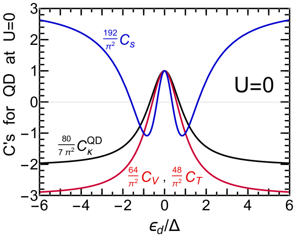
Figure 1: Coefficients $C_{V}$, $C_{T}$, $C_{S}$, and $C_{\kappa}^{\mathrm{QD}}$ for noninteracting $U=0$ quantum dots plotted vs $\epsilon_{d}$.

In the rest of this paper, we will demonstrate the behavior of the next leading order terms of the transport coefficients for $N=4$ and $6$. To this end, we calculate the correlation functions $\delta$, $\chi_{\sigma_{1}\sigma_{2}}$, and $\chi_{\sigma_{1}\sigma_{2}\sigma_{3}}^{[3]}$ with the NRG approach Hewson et al. (2004); Teratani et al. (2020a), specifically using Eqs. (42)–(45) for the three-body correlations. We have reported the NRG results for the coefficient $C_{V}$ in the previous paper for studying the role of bias and tunneling asymmetries on the nonlinear terms of $dJ/dV$ at $T=0$.Tsutsumi et al. (2023) In this paper, we provide a comprehensive view on the three-body Fermi-liquid effect, through a systematic analysis of the next-leading order terms $C_{S}$, $C_{T}$, and $C_{\kappa}^{\mathrm{QD}}$ for quantum dots, and through the related coefficients for magnetic alloys, $C_{\varrho}^{\mathrm{MA}}$, and $C_{\kappa}^{\mathrm{MA}}$ described in Sec.  IX.

V.4 Numerical renormalization group approach

We have carried out NRG calculations, dividing the $N$ conduction channels into $N/2$ pairs and using the SU(2) spin and U(1) charge symmetries for each of the pairs, i.e.  $\prod_{k=1}^{\frac{N}{2}}\left\{\mbox{SU(2)}\otimes\mbox{U(1)}\right\}_{k}$ symmetries. The discretization parameter $\Lambda$ and the number of retained low-lying excited states $N_{\mathrm{trunc}}$ are chosen such that $(\Lambda,N_{\mathrm{trunc}})=(6,10000)$ for $N=4$, and $\,(20,30000)$ for $N=6$.

In particular, for $N=6$, we have exploited the method of Stadler et al.Stadler et al. (2016) The truncation procedure is introduced at each of the steps ($k=$1, $2$, $\ldots$, $N/2$) after adding the states constructed with one of the channel pairs, using Olivera’s $\mathcal{Z}$-trickOliveira and Oliveira (1994) choosing different $\mathcal{Z}$ values for each of the $N/2$ steps: $\mathcal{Z}_{k}=1/2+k/N$ for the $k$-th pair. This method significantly reduces the numerical cost to calculate the low-lying energy state, and enables us to deduce the Fermi-liquid parameters for the $N=6$ Anderson impurity model.

VI Three-body correlations in the SU(4) $\&$ SU(6) Anderson impurity

We have reported part of the NRG results for the two-body and three-body correlation functions in the previous paper,Tsutsumi et al. (2023) for interaction strengths up to $U/(\pi\Delta)=5.0$. In order to quickly grasp the underlying physics derived from quasiparticle properties in the SU(4) and SU(6) cases, we provide a brief review of the key characteristics of the two-body correlation functions in Appendix D, extending the interaction range up to $U/(\pi\Delta)=6.0$. Additionally, we also present the NRG results for the renormalized resonance-level position $\widetilde{\epsilon}_{d\sigma}$, which has not been examined previously.

In this section, we consider the behavior of charge and spin susceptibilities defined in Eqs. (37) and (41). In particular, we focus on the derivatives $\partial\overline{\chi}_{C}/\partial\epsilon_{d}$ and $\partial\overline{\chi}_{S}/\partial\epsilon_{d}$, which can also be expressed in terms of the three-body correlation functions:

$$\frac{\partial\overline{\chi}_{C}}{\partial\epsilon_{d}}\,= \ \chi_{\sigma\sigma\sigma}^{[3]}\,+\,3\,\widetilde{\chi}_{\sigma\sigma^{\prime}\sigma^{\prime}}^{[3]}\,+\,2\,\widetilde{\chi}_{\sigma\sigma^{\prime}\sigma^{\prime\prime}}^{[3]}\;,$$ (55)

$$\frac{\partial\overline{\chi}_{S}}{\partial\epsilon_{d}}\,= \ \chi_{\sigma\sigma\sigma}^{[3]}\,+\,\frac{N-3}{N-1}\,\,\widetilde{\chi}_{\sigma\sigma^{\prime}\sigma^{\prime}}^{[3]}\,-\,\frac{2}{N-1}\,\,\widetilde{\chi}_{\sigma\sigma^{\prime}\sigma^{\prime\prime}}^{[3]}\,.$$ (56)

The NRG results reveal the fact that the derivatives in the left-hand side are suppressed in the strong-coupling region $|\xi_{d}|\lesssim(N-1)U/2$ for large $U$. It means that the linear combinations of the three-body correlations in left-hand side of Eqs. (55) and (56) approach zero and the number of independent components of $\chi_{\sigma_{1}\sigma_{2}\sigma_{3}}^{[3]}$ is reduced, as demonstrated below.

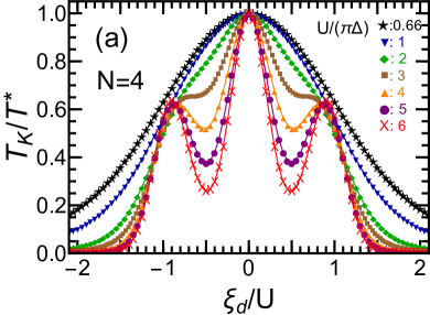
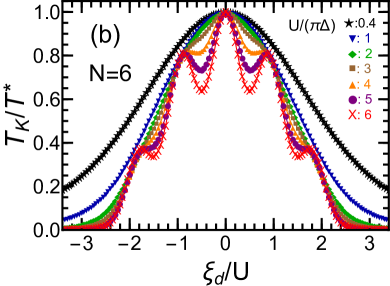
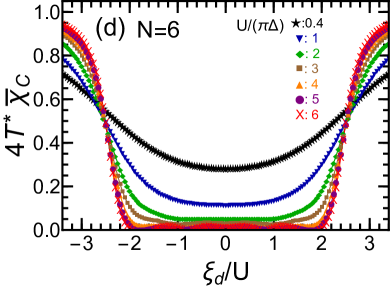
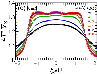
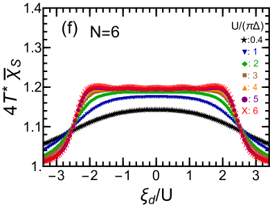
Figure 2: Inverse energy scale $1/T^{*}$, charge susceptibility $\overline{\chi}_{C}$ and spin $\overline{\chi}_{S}$ susceptibilities are plotted vs $\xi_{d}$ ($=\epsilon_{d}+U/2$) for $N=4$ and $6$. Here, $4T^{*}$ ($=1/\chi_{\sigma\sigma}$), and $T_{K}\equiv T^{*}\big{|}_{\xi_{d}=0}$. Interaction strengths are chosen such that, for $N=4$, $U/(\pi\Delta)=2/3(\star)$, $1(\blacktriangledown)$, $2(\blacklozenge)$, $3(\blacksquare)$, $4(\blacktriangle)$, $5(\bullet)$, and $6(\times)$, at which $T_{K}/(\pi\Delta)=0.20$, $0.18$, $0.13$, $0.092$, $0.063$, $0.041$, and $0.026$, respectively. For $N=6$, $U/(\pi\Delta)=2/5(\star)$, $1(\blacktriangledown)$, $2(\blacklozenge)$, $3(\blacksquare)$, $4(\blacktriangle)$, $5(\bullet)$, and $6(\times)$, at which $T_{K}/(\pi\Delta)=0.22$, $0.19$, $0.15$, $0.13$, $0.10$, $0.085$, and $0.068$, respectively.

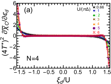
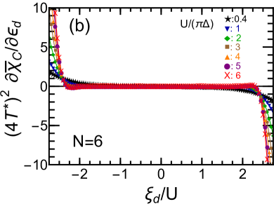
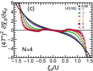
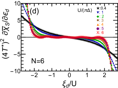
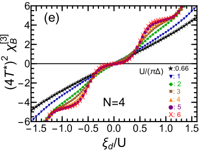
Figure 3: $(4T^{*})^{2}\partial\overline{\chi}_{C}/\partial\epsilon_{d}$, $(4T^{*})^{2}\partial\overline{\chi}_{S}/\partial\epsilon_{d}$, and $(4T^{*})^{2}\chi_{B}^{[3]}$ are plotted vs $\xi_{d}$ for $N=4$ and $6$. Interaction strengths are chosen such that, for $N=4$, $U/(\pi\Delta)=2/3(\star)$, $1(\blacktriangledown)$, $2()$, $3(\blacksquare)$, $4(\blacktriangle)$, $5(\bullet)$, $6(\times)$. For $N=6$, $U/(\pi\Delta)=2/5(\star)$, $1(\blacktriangledown)$, $2(\blacklozenge)$, $3(\blacksquare)$, $4(\blacktriangle)$, $5(\bullet)$, $6(\times)$.

VI.1 Charge and spin susceptibilities: $\overline{\chi}_{C}$ & $\overline{\chi}_{S}$

One of the most fundamental quantities which play a central role in the low-energy physics of quantum impurities is the characteristic energy scale $T^{*}\equiv 1/(4\chi_{\sigma\sigma})$, defined in Eq. (34) as an inverse of the diagonal susceptibility $N\chi_{\sigma\sigma}=\overline{\chi}_{C}+(N-1)\overline{\chi}_{S}$. We will use, in the following discussions, the Kondo temperature $T_{K}\equiv T^{*}\big{|}_{\xi_{d}=0}$, defined as the value of $T^{*}$ at the electron-hole symmetric point $\xi_{d}=0$.

The NRG results for $1/T^{*}$ in the SU(4) and SU(6) cases are plotted vs $\xi_{d}$ in Figs.  2(a) and 2(b), respectively, by multiplying them by $T_{K}$. We see that $1/T^{*}$ has $N-1$ local maxima for strong interactions, at integer-filling points, i.e., $\xi_{d}\simeq 0,\pm U,\ldots,\pm(N-2)U/2$, reflecting the oscillatory behavior of the wave function renormalization factor $z$ ($=\rho_{d\sigma}/\chi_{\sigma\sigma}$) described in Appendix D. At $|\xi_{d}|\gg(N-1)U/2$, the energy scale $T^{*}$ approaches the non-interacting value, $T_{K}/T^{*}\xrightarrow{\,|\xi_{d}|\gg(N-1)U/2\,}\Delta^{2}/\xi_{d}^{2}$, as the electron filling of the impurity levels approaches $N_{d}\simeq 0$ or $N$.

The charge susceptibilities for $N=4$ and $6$ are plotted in Figs. 2(c) and 2(d), using $T^{*}$ as a normalization factor, i.e., $4T^{\ast}\overline{\chi}_{C}=1-\widetilde{K}$ from Eq. (37). Therefore, the normalized value $4T^{\ast}\overline{\chi}_{C}$ is determined by the rescaled Wilson ratio $\widetilde{K}$, described in Appendix D. As $U$ increases, $4T^{\ast}\overline{\chi}_{C}$ decreases in a wide region of the impurity level $|\xi_{d}|\lesssim(N-1)U/2$, where the impurity levels are partially filled $1\lesssim N_{d}\lesssim N-1$. In this filling range, the charge susceptibility is significantly suppressed by the Coulomb repulsion, and it vanishes $4T^{\ast}\overline{\chi}_{C}\xrightarrow{\,U\gg\pi\Delta\,}0$ in the strong interaction limit. Outside this region, i.e., at $|\xi_{d}|\gg(N-1)U/2$, the charge susceptibility approaches the noninteracting value $4T^{*}\overline{\chi}_{C}\xrightarrow{\,|\xi_{d}|\to\infty\,}1$ as the filling of the impurity levels approaches $N_{d}\simeq 0$ or $N$.

Figures 2(e) and 2(f) show the spin susceptibilities for $N=4$ and $6$, which are normalized with the same scaling factor, i.e., $4T^{*}\overline{\chi}_{S}=1+\widetilde{K}/(N-1)$ [see Eq. (41)]. As the interaction $U$ increases, $4T^{*}\overline{\chi}_{S}$ increases from the non-interacting value $1$. In the strong interaction limit, it approaches the value $4T^{*}\overline{\chi}_{S}\to N/(N-1)$, i.e., $4/3$ for $N=4$ and $6/5$ for $N=6$, and exhibits a wide plateau structure in the strong-coupling region $|\xi_{d}|\lesssim(N-1)U/2$. At $|\xi_{d}|\gg(N-1)U/2$, where the occupation number approaches $N_{d}\simeq 0$ or $N$, the spin susceptibility also approaches the noninteracting value $4T^{*}\overline{\chi}_{S}\xrightarrow{\,|\xi_{d}|\to\infty\,}1$.

VI.2 Derivative of $\overline{\chi}_{C}$ and $\overline{\chi}_{S}$ with respect to $\epsilon_{d}$

The three-body correlation functions can be obtained from the derivatives of $\chi_{\sigma_{1}\sigma_{2}}$ with respect to $\epsilon_{d}$ and $b$, using Eqs. (42)–(44). In particular, $\partial\chi_{\sigma_{1}\sigma_{2}}/\partial\epsilon_{d}$ can be rewritten in terms of the derivatives of the charge and spin susceptibilities, as

$$\frac{\partial\chi_{\sigma\sigma}}{\partial\epsilon_{d}}\,= \ \frac{1}{N}\frac{\partial\overline{\chi}_{C}}{\partial\epsilon_{d}}\,+\,\frac{N-1}{N}\frac{\partial\overline{\chi}_{S}}{\partial\epsilon_{d}}\,,$$ (57)

$$(N-1)\frac{\partial\chi_{\sigma\sigma^{\prime}}}{\partial\epsilon_{d}}\,= \ \frac{N-1}{N}\frac{\partial\overline{\chi}_{C}}{\partial\epsilon_{d}}\,-\,\frac{N-1}{N}\frac{\partial\overline{\chi}_{S}}{\partial\epsilon_{d}}\,,$$ (58)

for $\sigma\neq\sigma^{\prime}$. Figures 3(a) and 3(b) show the NRG results for $\partial\overline{\chi}_{C}/\partial\epsilon_{d}$ for $N=4$ and $6$, respectively. Similarly, the derivative of the spin susceptibility $\partial\overline{\chi}_{S}/\partial\epsilon_{d}$ for $N=4$ and $6$ are plotted in Figs. 3 (c) and 3(d). Note that in these figures, the derivatives have been multiplied by a factor of $(4T^{*})^{2}$ to make them dimensionless. These derivatives are significantly suppressed in the strong-coupling region $|\xi_{d}|\lesssim(N-1)U/2$ for large $U$. More specifically, $|\partial\overline{\chi}_{C}/\partial\epsilon_{d}|\ll|\partial\overline{\chi}_{S}/\partial\epsilon_{d}|\ll 1/(4T^{*})^{2}$: the derivative of spin susceptibility becomes much smaller than $1/(4T^{*})^{2}$ while it is still larger than the derivative of charge susceptibility. Therefore, both $\partial\chi_{\sigma\sigma}/\partial\epsilon_{d}$ and $\partial\chi_{\sigma\sigma^{\prime}}/\partial\epsilon_{d}$ are suppressed in a wide range of electron fillings $1\lesssim N_{d}\lesssim N-1$ for large $U$.

We next consider $\chi_{B}^{[3]}$, defined in Eq. (45) as a derivative of a linear combination of the two different diagonal susceptibilities with respective to the magnetic fields $b$. Figures 3(e) and 3(f) show $(4T^{*})^{2}\chi_{B}^{[3]}$ for $N=4$ and $6$, respectively. We see that $(4T^{*})^{2}\chi_{B}^{[3]}$ exhibits a staircase structure with a flat plateau emerging around the integer filling points $\xi_{d}=0$, $\pm U$, $\pm 2U$, $\ldots$, $(N-2)U/2$ for large $U$. The magnitude $\bigl{|}\chi_{B}^{[3]}\bigr{|}$ becomes much larger than the derivative of the charge and spin susceptibilities, $|\partial\overline{\chi}_{C}/\partial\epsilon_{d}|$ and $|\partial\overline{\chi}_{S}/\partial\epsilon_{d}|$. Therefore, $\chi_{B}^{[3]}$ dominates the terms in the right-hand side of Eqs. (42)–(44) in the strong-coupling region $|\xi_{d}|\lesssim(N-1)U/2$, and the three independent components of three-body correlations approach one another in such a way that

$$\chi_{\sigma\sigma\sigma}^{[3]}\,\simeq\,-\,\widetilde{\chi}_{\sigma\sigma^{\prime}\sigma^{\prime}}^{[3]}\,\simeq\,\widetilde{\chi}_{\sigma\sigma^{\prime}\sigma^{\prime\prime}}^{[3]}\ \simeq\ -\frac{N-1}{N}\,\chi_{B}^{[3]}\,.$$ (59)

This means that the three-body correlations are described by a single parameter $\chi_{B}^{[3]}$ in a wide filling range $1\lesssim N_{d}\lesssim N-1$ for large $U$.

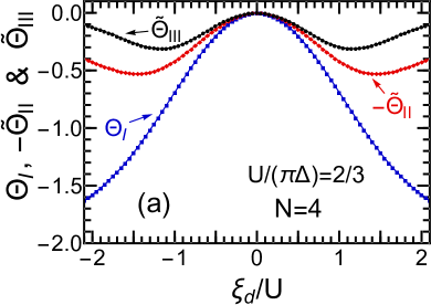
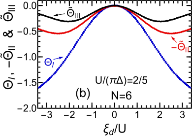
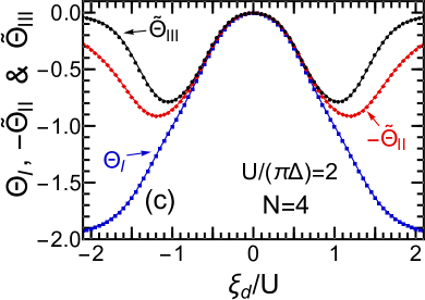
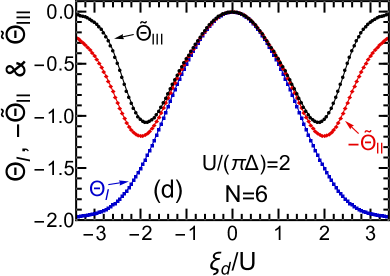
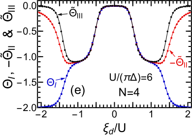
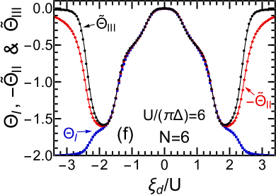
Figure 4: Dimensionless three-body corrections $\Theta_{\mathrm{I}}(\blacksquare)$ , $-\widetilde{\Theta}_{\mathrm{II}}(\blacklozenge)$, and $\widetilde{\Theta}_{\mathrm{III}}(\bullet)$ are plotted vs $\xi_{d}$, for interaction strengths $U/(\pi\Delta)=2/3$ (a), $2/5$ (b), $2$ (c,d), and $6$ (e,f).

VI.3 Three-body correlations for $N=4$ and $6$

We have calculated the three-body correlation functions $\chi_{\sigma\sigma\sigma}^{[3]}$, $\widetilde{\chi}_{\sigma\sigma^{\prime}\sigma^{\prime}}^{[3]}$ and $\widetilde{\chi}_{\sigma\sigma^{\prime}\sigma^{\prime\prime}}^{[3]}$ for $\sigma\neq\sigma^{\prime}\neq\sigma^{\prime\prime}\neq\sigma$, using Eqs. (42)–(44). Figure 4 shows the dimensionless three-body correlations $\Theta_{\mathrm{I}}$, $\widetilde{\Theta}_{\mathrm{II}}$ and $\widetilde{\Theta}_{\mathrm{III}}$, defined in Eqs.  (48) and (49). The left and right panels describe the NRG results in the SU(4) and SU(6) cases, respectively, and three deferent interaction strengths (from weak to strong) are chosen for the top, middle, and bottom panels.

All components of the three-body correlation functions vanish $\Theta_{\mathrm{I}}=\widetilde{\Theta}_{\mathrm{II}}=\widetilde{\Theta}_{\mathrm{III}}=0$ at the electron-hole symmetric point at $\xi_{d}=0$, and evolve as $\xi_{d}$ deviates from this point. Among the three independent components, the intra-level component $\Theta_{\mathrm{I}}$ has the largest magnitude, and exhibits the plateau structures for large $U$ at integer filling points $N_{d}\simeq 1$ , $2$, $\ldots$, $N-1$. The other components, $\widetilde{\Theta}_{\mathrm{II}}$ and $\widetilde{\Theta}_{\mathrm{III}}$, involve inter-level correlations and evolve as the Coulomb interaction $U$ increases. In particular, the correlation between the three different levels $\widetilde{\Theta}_{\mathrm{III}}$ becomes the weakest. In the limit of $|\xi_{d}|\to\infty$, the diagonal component $\Theta_{\mathrm{I}}$ approaches the noninteracting value while the other two vanish:

$$\Theta_{\mathrm{I}}\,\xrightarrow{|\xi_{d}|\to\infty\,}\,-2,\quad\widetilde{\Theta}_{\mathrm{II}}\,\xrightarrow{|\xi_{d}|\to\infty\,}\,0,\quad\widetilde{\Theta}_{\mathrm{III}}\,\xrightarrow{|\xi_{d}|\to\infty\,}\,0.$$ (60)

Figures 4(e) and 4(f) clearly demonstrate the relation Eq. (59), which holds at $|\xi_{d}|\lesssim(N-1)U/2$ for large $U$:

$$\Theta_{\mathrm{I}}\,\simeq\,-\widetilde{\Theta}_{\mathrm{II}}\,\simeq\,\widetilde{\Theta}_{\mathrm{III}}\,.$$ (61)

It means that all the three-body components are determined by a single parameter $\chi_{B}^{[3]}$ in the strong-coupling region for large $U$, as mentioned. The dimensionless three-body functions clearly exhibit the plateau structure around the integer filling points $\xi_{d}=0$, $\pm U$, $\pm 2U$, $\ldots$, $\pm(N-2)U/2$, where the SU($N$) Kondo effect occurs. These structures reflect the behavior of $\chi_{B}^{[3]}$, described in Figs. 3(e) and 3(f), and evolve as the interaction strength $U$ increases. We see, in Figs.  4(e) and 4(f), that the plateaus appear much clearer for $N=4$ than for $N=6$, for the same interaction strength $U/(\pi\Delta)=6.0$.

We will examine, in the proceeding sections, how these three-body correlation functions affect the next-leading order terms of the transport coefficients in the low-energy Fermi-liquid regime away from half filling.

VII Nonlinear current noise of
SU(4) $\&$ SU(6) quantum dots

In this section, we discuss the nonlinear terms of the steady current $J$ and the current noise $S_{\mathrm{noise}}^{\mathrm{QD}}$, specifically the terms of order $(eV)^{3}$, for symmetric junctions with $\Gamma_{L}=\Gamma_{R}$ and $\mu_{L}=-\mu_{R}={eV}/{2}$. In order to give a comprehensive view on the low-bias behavior of these terms, we start our discussions with a brief review of the previous results for the coefficient $C_{V}$ of the nonlinear conductance,Tsutsumi et al. (2023) extending slightly the interaction range up to $U/(\pi\Delta)=6.0$. We will then discuss the results for $C_{S}$, i.e., the order $|eV|^{3}$ term of nonlinear noise.

VII.1 $C_{V}$: order $(eV)^{2}$ term of $dJ/dV$

The leading-order term of the conductance, at $T=0$, is determined by the transmission probability $\sin^{2}\delta$, i.e., the first term in the right hand-side of Eq. (51). It exhibits the well-known Kondo plateaus, which develop in the strong-coupling region, as shown in Figs. 14(b) and 15(b) in Appendix D.

The next-leading order term $C_{V}$ of the nonlinear conductance can be decomposed into the two-body part $W_{V}$, defined in table 2, and the three-body part $\Theta_{V}$, as

$$C_{V}\,=\,\frac{\pi^{2}}{64}\,\bigl{(}W_{V}+\Theta_{V}\bigr{)},\qquad\Theta_{V}\,\equiv\,\Theta_{\mathrm{I}}+3\,\widetilde{\Theta}_{\mathrm{II}}.$$ (62)

These coefficients $C_{V}$, $W_{V}$ and $\Theta_{V}$ are plotted vs $\xi_{d}$ in Figs. 5(a)–5(f) for $N=4$ and $6$.

The two-body part $W_{V}$ dominates the next-leading order term near the electron-hole symmetric point $\xi_{d}=0$, where $\delta=\pi/2$ and the three-body part $\Theta_{V}$ vanishes:

$$W_{V}\,\xrightarrow{\,\xi_{d}=0}\,1+\frac{5\widetilde{K}^{2}}{N-1},\qquad\Theta_{V}\xrightarrow{\,\xi_{d}=0\,}0.$$ (63)

Therefore, in the strong interaction limit, the peak at $\xi_{d}=0$ reaches $(64/\pi^{2})C_{V}\xrightarrow{\,\xi_{d}=0\,\&U\to\infty}8/3$ and $2$ for $N=4$ and $6$, respectively. Note that the rescaled Wilson ratio approaches $\widetilde{K}\simeq 1$ in a wide region of $|\xi_{d}|\lesssim(N-1)U/2$ for large $U$. Outside this region, the two-body and three-body parts of $C_{V}$ approach to the noninteracting values,

$$W_{V}\,\xrightarrow{\,|\xi_{d}|\to\infty}\,-1,\qquad\Theta_{V}\,\xrightarrow{\,|\xi_{d}|\to\infty}\,-2,$$ (64)

since $\cos 2\delta\xrightarrow{\,|\xi_{d}|\to\infty}1$, $\widetilde{K}\xrightarrow{\,|\xi_{d}|\to\infty}0$, and the three-body contributions approach the values given in Eq. (60).

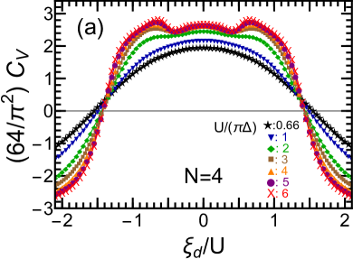
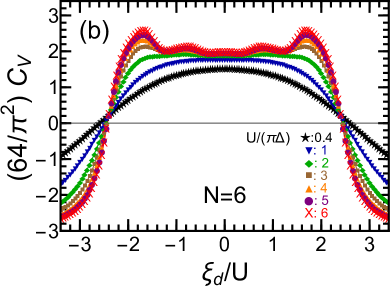
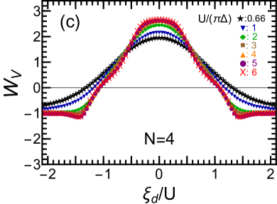
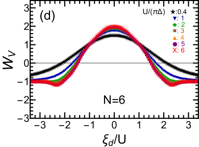
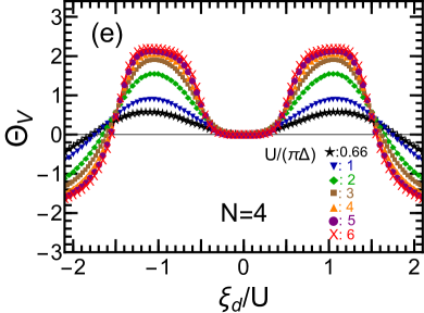
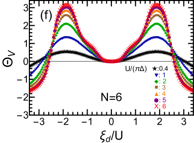
Figure 5: $\xi_{d}$ dependence of $C_{V}=(\pi^{2}/64)(W_{V}+\Theta_{V})$, two-body part $W_{V}$, and three-body part $\Theta_{V}\equiv\Theta_{\mathrm{I}}+3\,\widetilde{\Theta}_{\mathrm{II}}$. Left panels: $N=4$, for $U/(\pi\Delta)=2/3(\star)$, $1(\blacktriangledown)$, $2(\blacklozenge)$, $3(\blacksquare)$, $4(\blacktriangle)$, $5(\bullet)$, $6(\times)$. Right panels: $N=6$, for $U/(\pi\Delta)=2/5(\star)$, $1(\blacktriangledown)$, $2(\blacklozenge)$, $3(\blacksquare)$, $4(\blacktriangle)$, $5(\bullet)$, $6(\times)$.

The SU($N$) Kondo effect occurs in the strong-coupling region $|\xi_{d}|\lesssim(N-1)U/2$ at the integer filling points. The plateau structure evolves as $U$ increases, especially in the three-body part $\Theta_{V}$, as seen in Figs. 5(e) and 5(f). In the strong-coupling region, it can be expressed in the form $\Theta_{V}\simeq-2\Theta_{\mathrm{I}}$ due to Eq. (61). The two body part $W_{V}$, shown in Figs. 5(c) and 5(d) for $U/(\pi\Delta)\leq 6.0$, does not exhibit a clear plateau other than the one appearing near half filling. For $N=4$, this is because the factor $\cos 2\delta$ for $W_{V}$ vanishes at $\delta=\pi/4$ and $3\pi/4$, i.e., at the quarter and three-quarters filling points. As a sum of $W_{V}$ and $\Theta_{V}$, the coefficient $C_{V}$ exhibits a wide and rather flat structure in the region of $|\xi_{d}|\lesssim(N-1)U/2$ for large $U$, seen in Figs. 5(a) and 5(b). There also emerge some weak local maxima in this flat structure at the integer filling points $\xi_{d}=0$, $\pm U$, $\pm 2U$, $\ldots$, $\pm(N-2)U/2$. In particular, the peak is most pronounced at $\xi_{d}\simeq\pm(N-2)U/2$, where $N_{d}\simeq 1$ or $N-1$.

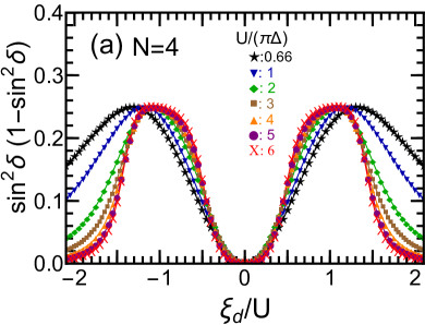
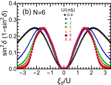
Figure 6: Linear part, $\sin^{2}\delta\,(1-\sin^{2}\delta)$, of the noise $S_{\mathrm{noise}}^{\mathrm{QD}}$. Interaction strengths are chosen for (a) $N=4$ to be $U/(\pi\Delta)=2/3(\star)$, $1(\blacktriangledown)$, $2(\blacklozenge)$, $3(\blacksquare)$, $4(\blacktriangle)$, $5(\bullet)$, $6(\times)$. For (b) $N=6$, $U/(\pi\Delta)=2/5(\star)$, $1(\blacktriangledown)$, $2(\blacklozenge)$, $3(\blacksquare)$, $4(\blacktriangle)$, $5(\bullet)$, $6(\times)$.

VII.2 Linear and order $|eV|^{3}$ nonlinear parts of $S_{\mathrm{noise}}^{\mathrm{QD}}$

We next consider the current noise $S_{\mathrm{noise}}^{\mathrm{QD}}$, the low-energy asymptotic form of which is given in Eq. (52) and table 2. The leading-order term, $\sin^{2}\delta\,(1-\sin^{2}\delta)=(1-\cos 4\delta)/8$, corresponds to the linear-response noise, the NRG results for which are shown as a function of $\xi_{d}$ in Figs. 6(a) and 6(b), for $N=4$ and $6$, respectively. The linear noise is maximized at the points where the phase shift reaches $\delta=\pi/4$ and $3\pi/4$. It occurs at the integer filling points $N_{d}=1$ and $3$ for $N=4$, at which the SU(4) Kondo effect makes the peaks wide and flat. In contrast, for $N=6$, the peak emerges at the half-integer filling points $N_{d}=3/2$ and $9/2$. More generally, the peak of the linear noise forms a flat plateau structure for $N\equiv 0$ (mod $4$), whereas the peak becomes round for $N\equiv 2$ (mod $4$) due to the fluctuations occurring between two adjacent integer filling states. For large $U$, the quarter and three-quarters fillings occur near $|\xi_{d}|/U\simeq N/4$, at which the ground state is highly correlated for multilevel systems of $N\geq 4$. In contrast, these fillings occur at $\xi_{d}\simeq\pm U/2$ for SU(2) quantum dots, where the electron correlation becomes less important due to the valence fluctuations (see Appendix E).

The coefficient $C_{S}$ for the order $|eV|^{3}$ term of current noise $S_{\mathrm{noise}}^{\mathrm{QD}}$ can also be decomposed into the two-body $W_{S}$ and three-body $\Theta_{S}$ parts, as shown in table 2:

$$\!\!C_{S}=\frac{\pi^{2}}{192}\bigl{(}W_{S}+\Theta_{S}\bigr{)},\quad\Theta_{S}\equiv-\bigl{(}\Theta_{\mathrm{I}}+3\widetilde{\Theta}_{\mathrm{II}}\bigr{)}\cos 2\delta.$$ (65)

The behavior of three-body part $\Theta_{S}$ can be deduced from the one for $dJ/dV$, i.e., $\Theta_{V}=\Theta_{\mathrm{I}}+3\widetilde{\Theta}_{\mathrm{II}}$ shown in Figs. 5(e) and 5(f), multiplying them by a factor of “$-\cos 2\delta$” which induces the modulations. One of the most distinctive features of $C_{S}$, compared to the other coefficients $C$’s listed in table 2, is that it depends upon the higher harmonics $\cos 4\delta$ and $\sin 4\delta$ with respect to the phase shift, which enter through not only through $W_{S}$ but $\Theta_{S}$: note that $\Theta_{\mathrm{I}}$ and $\widetilde{\Theta}_{\mathrm{II}}$ defined in Eq. (48) is proportional to the factor $\sin 2\delta$. As $\xi_{d}$ varies, these higher harmonics evolve continuously in the range $0\leq 4\delta\leq 4\pi$, simultaneously with the electron filling $0\leq N_{d}\leq N$. Figures 7(a)–7(f) show results for $C_{S}$, $W_{S}$, and $\Theta_{S}$ for $N=4$ and $6$.

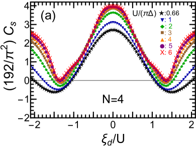
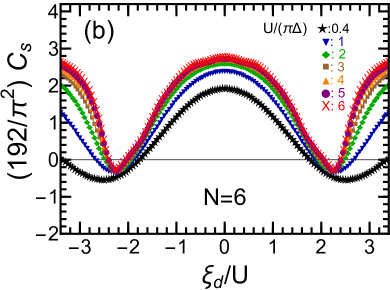
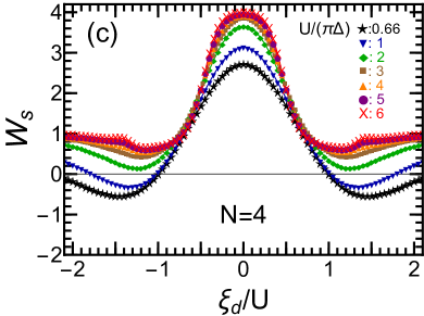
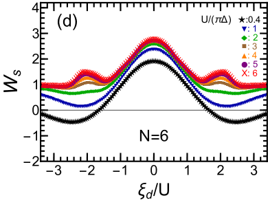
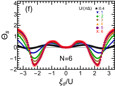
Figure 7: $\xi_{d}$ dependence of $C_{S}=(\pi^{2}/192)(W_{S}+\Theta_{S})$, two-body part $W_{S}$, and three-body part $\Theta_{S}\equiv-\bigl{(}\Theta_{\mathrm{I}}+3\,\widetilde{\Theta}_{\mathrm{II}}\bigr{)}\cos 2\delta$. Left panels: $N=4$, for $U/(\pi\Delta)=2/3(\star)$, $1(\blacktriangledown)$, $2(\blacklozenge)$, $3(\blacksquare)$, $4(\blacktriangle)$, $5(\bullet)$, $6(\times)$. Right panels: $N=6$, for $U/(\pi\Delta)=2/5(\star)$, $1(\blacktriangledown)$, $2(\blacklozenge)$, $3(\blacksquare)$, $4(\blacktriangle)$, $5(\bullet)$, $6(\times)$.

There are two valleys in each curve for $C_{S}$, shown in Figs. 7(a) and 7(b), at the valence fluctuation regions $\xi_{d}\simeq\pm(N-1)U/2$ for large $U$. These valleys rise all around as $U$ increases. In particular, for $N=4$, the value of $C_{S}$ at the bottom becomes positive for large interactions $U/(\pi\Delta)\gtrsim 5$, whereas for $N=6$ the bottom value remains still negative for the largest interaction $U/(\pi\Delta)=6$ examined here.

Near the electron-hole symmetric point $\xi_{d}=0$, where $\delta=\pi/2$ and $N_{d}=N/2$, the two-body part $W_{S}$ dominates the nonlinear noise $C_{S}$ since the three-body correlations disappear around this point:

$$W_{S}\,\xrightarrow{\,\xi_{d}=0\,}\,1+\frac{9\widetilde{K}^{2}}{N-1}\,,\qquad\Theta_{S}\xrightarrow{\,\xi_{d}=0\,}0.$$ (66)

In particular, in the limit of $U\to\infty$, the rescaled Wilson ratio approaches the saturation value $\widetilde{K}\to 1$. Hence, the coefficient for the order $|eV|^{3}$ term reaches $(192/\pi^{2})C_{S}\xrightarrow{\xi_{d}=0\,\&\,U\to\infty}4$ for $N=4$, and it reaches $14/5$ for $N=6$: the height of this ridge decreases as $N$ increases.

In contrast, in the opposite limit $|\xi_{d}|\to\infty$, the two-body and the three-body parts approach the noninteracting values

$$W_{S}\,\xrightarrow{\,|\xi_{d}|\to\infty}\,1,\qquad\Theta_{S}\,\xrightarrow{\,|\xi_{d}|\to\infty}\,2,$$ (67)

since $\cos 2\delta\to 1$, $\widetilde{K}\to 0$, and $\Theta_{\mathrm{I}}\to-2$ in this limit. Therefore, both $W_{S}$ and $\Theta_{S}$ give comparable contributions to $C_{S}$ in the region $|\xi_{d}|\gtrsim(N-1)U/2$, where the impurity levels are almost empty $N_{d}\simeq 0$ or fully occupied $N_{d}\simeq N$. In particular, we see in Figs. 7(c) and 7(d) that the two-body part approaches the saturation value $W_{S}\to 1$ already at $|\xi_{d}|\simeq(N-1)U/2$ for large interactions $U/(\pi\Delta)\gtrsim 3$.

In the strong-coupling region $|\xi_{d}|\lesssim(N-1)U/2$ for large $U$, the behavior of two-body part $W_{S}$ is determined by the higher-harmonic $\cos 4\delta$ term, as

$$W_{S}\,\simeq\,\frac{1}{2}\left(3+\frac{5}{N-1}\right)\,+\,\frac{1}{2}\left(\frac{13}{N-1}-1\right)\cos 4\delta\,,$$ (68)

since the Wilson ratio is locked at $\widetilde{K}\simeq 1.0$ in this region. We can see in Figs. 7(c) and 7(d) that the two-body part $W_{S}$ has local minima at quarter and three-quarters filling points, which occur at $\delta=\pi/4$ and $3\pi/4$, or $|\xi_{d}|/U\simeq N/4$ for large $U$. At these local minima, $W_{S}$ take a positive value for $N\geq 4$, as it can be deduced from Eq. (68). This is in contrast to the SU(2) case where the local minima of $W_{S}$ take a negative value, as shown in Appendix E. In the strong-coupling region $|\xi_{d}|\lesssim(N-1)U/2$, the three-body part takes the following form, for large $U$,

$$\Theta_{S}\,\simeq\,\frac{\chi_{\sigma\sigma\sigma}^{[3]}}{2\pi\,\chi_{\sigma\sigma}^{2}}\,\sin 4\delta\,,$$ (69)

due to the property described in Eq. (61). Equation (69) clearly shows that the three-body part vanishes, $\Theta_{S}=0$, at quarter $\delta=\pi/4$ and three-quarters $\delta=3\pi/4$ fillings. Therefore, at these filling points, $\Theta_{S}$ does not exhibit the plateau structures for $N=4$ in Fig. 7(e), in contrast to $\Theta_{V}$ which clearly exhibits the plateau structures as seen in Fig. 5(e). In contrast, for $N=6$, $\Theta_{S}$ shows the clear plateau structures in Fig. 7(f) at the fillings of $N_{d}=2$ and $4$. The three-body parts $\Theta_{S}$ for both $N=4$ and $6$ also have pronounced local minima near the valence fluctuation regions $\xi_{d}\simeq\pm(N-1)U/2$, which cause the valley structure appearing in $C_{S}$. Similar valley structure also emerges in $C_{S}$ for $N=2$, as shown in Appendix E. However, it stems from the two-body correlations $W_{S}$, instead of $\Theta_{S}$, in the SU($2$) case.

VIII Thermoelectric transport of
SU(4) $\&$ SU(6) quantum dots

We next consider the order $T^{2}$ term of the linear conductance $g=dJ/dV\big{|}_{eV=0}$ and the order $T^{3}$ term of thermal conductance $\kappa_{\mathrm{QD}}$ of SU($N$) quantum dots.

VIII.1 $C_{T}$: order $T^{2}$ term of $dJ/dV$

The coefficient $C_{T}$ for the order $T^{2}$ conductance, defined in table 2, also consists of two-body part $W_{T}$ and three-body part $\Theta_{T}$:

$$C_{T}\,=\,\frac{\pi^{2}}{48}\,\bigl{(}W_{T}+\Theta_{T}\bigr{)}\,,\qquad\Theta_{T}\,\equiv\,\Theta_{\mathrm{I}}+\widetilde{\Theta}_{\mathrm{II}}\,.$$ (70)

In particular, the three-body part $\Theta_{T}$ is solely determined by the derivatives of the charge and spin susceptibilities, given in Eqs. (55) and (56), and does not depend on $\chi_{B}^{[3]}$:

$$\Theta_{T}\,=\,\frac{(4T^{*})^{2}}{N}\left[\,\frac{\partial\overline{\chi}_{C}}{\partial\epsilon_{d}}\,+(N-1)\frac{\partial\overline{\chi}_{S}}{\partial\epsilon_{d}}\,\,\right]\frac{\sin 2\delta}{2\pi}\,.$$ (71)

This is a quite distinct characteristics of $C_{T}$ from the next-leading order terms of the other transport coefficients. Figures 8(a)–8(f) show the NRG results for $C_{T}$, $W_{T}$, and $\Theta_{T}$, obtained for the SU(4) and SU(6) symmetric cases.

We see in Figs. 8(e) and 8(f) that the three-body contribution almost vanishes, $\Theta_{T}\simeq 0.0$, in the wide strong-coupling region $|\xi_{d}|\lesssim(N-1)U/2$, in which the occupation number varies with $\xi_{d}$ in the range of $1\lesssim N_{d}\lesssim N-1$. This is because the magnitudes of the derivatives $\partial\overline{\chi}_{C}/\partial\epsilon_{d}$ and $\partial\overline{\chi}_{S}/\partial\epsilon_{d}$, appearing in the right-hand side of Eq. (71), are significantly suppressed by the Coulomb repulsion in this region, as demonstrated in Figs. 3(a)–3(d).

Therefore, the two-body part $W_{T}$ dominates $C_{T}$ in the strong-coupling region $|\xi_{d}|\lesssim(N-1)U/2$, and it takes the following form for large $U$,

$$W_{T}\simeq\left[\,1+\frac{2}{N-1}\,\right]\,(2\sin^{2}\delta-1),\qquad\Theta_{T}\simeq 0,$$ (72)

as the rescaled Wilson ratio reaches the saturation value $\widetilde{K}\to 1$. Hence, the plateau structure of $C_{T}$ is determined by the $\sin^{2}\delta$ term of $W_{T}$ in Eq. (72). In particular, the plateau around the half filling point $|\xi_{d}|\lesssim U/2$ reaches the height of $(48/\pi^{2})C_{T}\xrightarrow{U\to\infty\,}5/3$ and $7/5$ for $N=4$ and $6$, respectively, since $\delta\simeq\pi/2$ in this region. The order $T^{2}$ conductance, $C_{T}$, vanishes at $|\xi_{d}|/U\simeq N/4$, more specifically at the quarter and the three-quarter fillings where the phase shift reaches $\delta=\pi/4$ or $3\pi/4$. The zero points of $C_{T}$ emerge at integer fillings in the case of $N\equiv 0$ (mod $4$) at which the SU($N$) Kondo effect is occurring, whereas for $N\equiv 2$ (mod $4$) the zeros emerge at half-integer filings in between the two adjacent Kondo states. This explains the reason why the SU(4) Kondo state at quarter filling exhibits universal $T/T^{*}$-scaling behavior, which shows the $(T/T^{*})^{4}$ dependence at low temperatures instead of the $(T/T^{*})^{2}$ dependence Teratani et al. (2020b).

In the valence fluctuation and empty (or fully-occupied) orbital regimes, which spread over the regions of $|\xi_{d}|\gtrsim(N-1)U/2$, the tree-body part $\Theta_{T}$ becomes comparable to the two-body part $W_{T}$. Both of these parts approach the noninteracting values in the limit of $|\xi_{d}|\to\infty$:

$$W_{T}\,\xrightarrow{\,|\xi_{d}|\to\infty}\,-1,\qquad\Theta_{T}\,\xrightarrow{\,|\xi_{d}|\to\infty}\,-2.$$ (73)

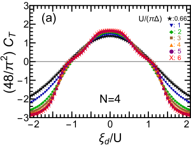
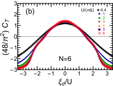
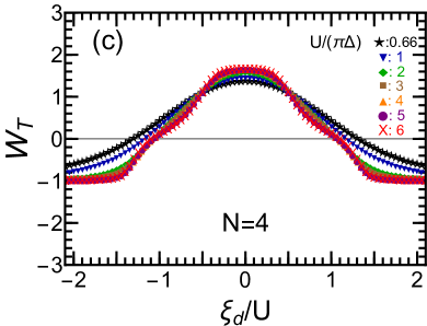
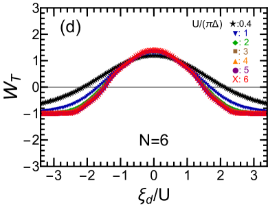
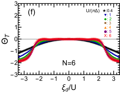
Figure 8: $\xi_{d}$ dependence of $C_{T}=(\pi^{2}/48)(W_{T}+\Theta_{T})$, two-body part $W_{T}$, and three-body part $\Theta_{T}\equiv\Theta_{\mathrm{I}}+3\,\widetilde{\Theta}_{\mathrm{II}}$. Left panels: $N=4$, for $U/(\pi\Delta)=2/3(\star)$, $1(\blacktriangledown)$, $2(\blacklozenge)$, $3(\blacksquare)$, $4(\blacktriangle)$, $5(\bullet)$, $6(\times)$. Right panels: $N=6$, for $U/(\pi\Delta)=2/5(\star)$, $1(\blacktriangledown)$, $2(\blacklozenge)$, $3(\blacksquare)$, $4(\blacktriangle)$, $5(\bullet)$, $6(\times)$.

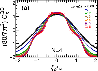
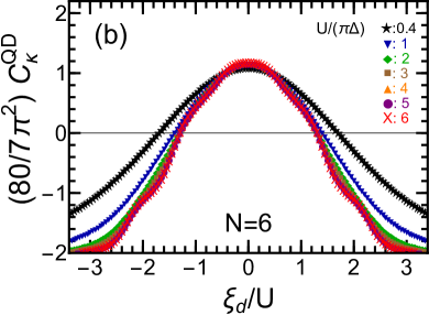
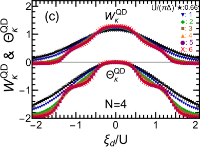
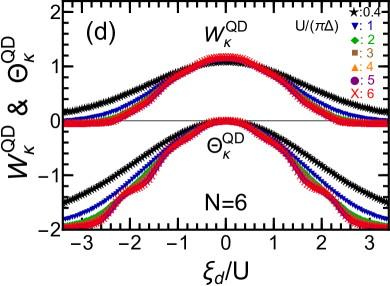
Figure 9: $\xi_{d}$ dependence of $C_{\kappa}^{\mathrm{QD}}=(7\pi^{2}/80)(W_{\kappa}^{\mathrm{QD}}+\Theta_{\kappa}^{\mathrm{QD}})$, two-body part $W_{\kappa}^{\mathrm{QD}}$, and three-body part $\Theta_{\kappa}^{\mathrm{QD}}=\Theta_{\mathrm{I}}+\frac{5}{21}\widetilde{\Theta}_{\mathrm{II}}$. Left panels: $N=4$, for $U/(\pi\Delta)=2/3(\star)$, $1(\blacktriangledown)$, $2(\blacklozenge)$, $3(\blacksquare)$, $4(\blacktriangle)$, $5(\bullet)$, $6(\times)$. Right panels: $N=6$, for $U/(\pi\Delta)=2/5(\star)$, $1(\blacktriangledown)$, $2(\blacklozenge)$, $3(\blacksquare)$, $4(\blacktriangle)$, $5(\bullet)$, $6(\times)$.

VIII.2 $C_{\kappa}^{\mathrm{QD}}$: order $T^{3}$ term of $\kappa_{\mathrm{QD}}$

The coefficient $C_{\kappa}^{\mathrm{QD}}$ for the order $T^{3}$ term of the thermal conductance $\kappa_{\mathrm{QD}}$ can also be decomposed into two parts, $W_{\kappa}^{\mathrm{QD}}$ and $\Theta_{\kappa}^{\mathrm{QD}}$, as shown in table 2:

$$C_{\kappa}^{\mathrm{QD}}\,=\,\frac{7\pi^{2}}{80}\,\bigl{(}W_{\kappa}^{\mathrm{QD}}+\Theta_{\kappa}^{\mathrm{QD}}\bigr{)},\qquad\Theta_{\kappa}^{\mathrm{QD}}\,\equiv\,\Theta_{\mathrm{I}}+\frac{5}{21}\widetilde{\Theta}_{\mathrm{II}}.$$ (74)

In contrast to $\Theta_{T}$ of the conductance given in Eq. (71), the three-body part $\Theta_{\kappa}^{\mathrm{QD}}$ of the thermal conductance depends on $\chi_{B}^{[3]}$ as well as $\partial\overline{\chi}_{C}/\partial\epsilon_{d}$ and $\partial\overline{\chi}_{S}/\partial\epsilon_{d}$. The contribution of $\chi_{B}^{[3]}$ enters through $\chi_{\sigma\sigma\sigma}^{[3]}$ and $\widetilde{\chi}_{\sigma\sigma^{\prime}\sigma^{\prime}}^{[3]}$, described in in Eqs. (42) and (43). This component $\chi_{B}^{[3]}$ yields the plateau structure in $\Theta_{\kappa}^{\mathrm{QD}}$, which reflects the staircase behavior seen in Figs. 3(e) and 3(f). Figure 9 shows the NRG results for $C_{\kappa}^{\mathrm{QD}}$, $W_{\kappa}^{\mathrm{QD}}$, and $\Theta_{\kappa}^{\mathrm{QD}}$ in the SU(4) and SU(6) cases.

Near half filling in the region of $|\xi_{d}|\lesssim U/2$, the two-body part $W_{\kappa}^{\mathrm{QD}}$ dominates $C_{\kappa}^{\mathrm{QD}}$ as the three-body part $\Theta_{\kappa}^{\mathrm{QD}}$ disappears near half filling $\xi_{d}=0$, i.e., $\delta=\pi/2$:

$$W_{\kappa}^{\mathrm{QD}}\xrightarrow{\,\xi_{d}=0\,}\,1+\frac{6\widetilde{K}^{2}}{7(N-1)}\,,\qquad\Theta_{\kappa}^{\mathrm{QD}}\xrightarrow{\,\xi_{d}=0\,}0\,.$$ (75)

In particular, in the strong interaction limit $U\to\infty$, and the coefficient $C_{\kappa}^{\mathrm{QD}}$ for $N=4$ and $6$ approach the values of $[80/(7\pi^{2})]C_{\kappa}^{\mathrm{QD}}\xrightarrow{\,\xi_{d}=0\,\&\,U\to\infty\,}9/7$ and $41/35$, respectively.

The rescaled Wilson ratio takes the values very close to the satulation value $\widetilde{K}\to 1$ for large $U$ in the strong-coupling region of $|\xi_{d}|\lesssim(N-1)U/2$, as desribed in Appendix D. Similarly, in this region, the three-body correlations show the property described in Eq. (61), and thus $W_{\kappa}^{\mathrm{QD}}$ and $\Theta_{\kappa}^{\mathrm{QD}}$ take the form

$$W_{\kappa}^{\mathrm{QD}}\,\simeq \ \frac{1}{21}\left[10+\left(11+\frac{18}{N-1}\right)\left(2\sin^{2}\delta-1\right)\right],$$

$$\Theta_{\kappa}^{\mathrm{QD}}\,\simeq \ \frac{16}{21}\,\Theta_{\mathrm{I}}\,.$$ (76)

Therefore, the plateau structure of $W_{\kappa}^{\mathrm{QD}}$ is determined by the $\sin^{2}\delta$ term appearing in the right-hand side while the structure of $\Theta_{\kappa}^{\mathrm{QD}}$ reflects the behavior of $\Theta_{\mathrm{I}}$ shown in Fig. 4(e) and 4(f). The coefficient $C_{\kappa}^{\mathrm{QD}}$ changes sign in the strong-coupling region at two points of $\xi_{d}$, which are incommensurate with the occupation number $N_{d}$ in contrast to $C_{T}$ that changes sign at $1/4$ and $3/4$ fillings.

In the opposite limit $|\xi_{d}|\to\infty$, both the two-body and three-body parts approach the noninteracting values,

$$W_{\kappa}^{\mathrm{QD}}\xrightarrow{\,|\xi_{d}|\to\infty\,}\,-\frac{1}{21},\qquad\Theta_{\kappa}^{\mathrm{QD}}\xrightarrow{\,|\xi_{d}|\to\infty\,}\,-2.$$ (77)

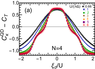
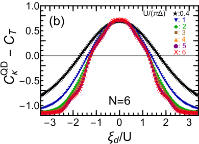
Figure 10: Order $T^{2}$ term $C_{L}^{\mathrm{QD}}=C_{\kappa}^{\mathrm{QD}}-C_{T}$ of Lorenz number $L_{\mathrm{QD}}$ is plotted vs $\xi_{d}$. Left panel: $N=4$, for $U/(\pi\Delta)=2/3(\star)$, $1(\blacktriangledown)$, $2(\blacklozenge)$, $3(\blacksquare)$, $4(\blacktriangle)$, $5(\bullet)$, $6(\times)$. Right panel: $N=6$, for $U/(\pi\Delta)=2/5(\star)$, $1(\blacktriangledown)$, $2(\blacklozenge)$, $3(\blacksquare)$, $4(\blacktriangle)$, $5(\bullet)$, $6(\times)$.

VIII.3 $C_{L}^{\mathrm{QD}}$: order $T^{2}$ term of $L_{\mathrm{QD}}$

The Lorenz number $L_{\mathrm{QD}}\equiv\kappa_{\mathrm{QD}}/(g\,T)$ for quantum dots is defined as the ratio of the thermal conductance $\kappa_{\mathrm{QD}}/T$ to the electrical conductance $g$. It takes the universal Wiedemann-Franz value at zero temperature: $L_{\mathrm{QD}}\xrightarrow{T\to 0}\pi^{2}/(3e^{2})$. However, as the temperature rises, it deviates from the universal value, showing the $T^{2}$ dependence described in tables 1 and 2. The coefficient for the order $T^{2}$ term is given by $C_{L}^{\mathrm{QD}}=C_{\kappa}^{\mathrm{QD}}-C_{T}$, as a difference between the next leading order terms of $\kappa_{\mathrm{QD}}/T$ and $g$.

Figure 10(a) and 10(b) show the NRG results for $C_{L}^{\mathrm{QD}}$ in the SU(4) and SU(6) cases, respectively. Near half filling $|\xi_{d}|\lesssim U/2$, the coefficient $C_{L}^{\mathrm{QD}}$ is determined by the two-body part $W_{L}^{\mathrm{QD}}$ as the three-body part $\Theta_{L}^{\mathrm{QD}}\equiv 16\,\Theta_{\mathrm{I}}$ vanishes at $\xi_{d}=0$, as seen in Fig. 4(e) and 4(f):

$$C_{L}^{\mathrm{QD}}\xrightarrow{\,\xi_{d}=0\,}\,\frac{\pi^{2}}{30}\left(2+\frac{\widetilde{K}^{2}}{N-1}\right)\ >0\,.$$ (78)

It takes a positive value and reaches $C_{L}^{\mathrm{QD}}\xrightarrow{\xi_{d}=0\,\&\,U=\infty}0,767\cdots$ for $N=4$, and $0.723\cdots$ for $N=6$, in the limit of $U\to\infty$ where $\widetilde{K}\to 1$.

In the strong-coupling region $|\xi_{d}|\lesssim(N-1)U/2$, the coefficient $C_{L}^{\mathrm{QD}}$ exhibits the plateau structures for large $U$, reflecting the corresponding structures of $C_{T}$ and $C_{\kappa}^{\mathrm{QD}}$. The coefficient $C_{L}^{\mathrm{QD}}$ changes sign at the points where the order $T^{2}$ terms of $\kappa_{\mathrm{QD}}/T$ and $g$ coincide, i.e., $C_{\kappa}^{\mathrm{QD}}=C_{T}$.

In the other regions at $|\xi_{d}|\gtrsim(N-1)U/2$, the impurity levels approach the empty $N_{d}\simeq 0$ or fully occupied $N_{d}\simeq N$ states. In particular, in the limit of $|\xi_{d}|\to\infty$, both the two-body and three-body parts approach the noninteracting values, $W_{L}^{\mathrm{QD}}\xrightarrow{|\xi_{d}|\to\infty}4$ and $16\Theta_{\mathrm{I}}\xrightarrow{|\xi_{d}|\to\infty}-32$, and thus

$$C_{L}^{\mathrm{QD}}\xrightarrow{\,|\xi_{d}|\to\infty\,}\,-\frac{7\pi^{2}}{60}\ =\ -1.151\cdots\ \ <0\,.$$ (79)

IX Fermi-liquid description for
SU($N$) symmetric magnetic alloys

We have discussed, in the previous sections, low-energy transport properties of the SU($N$) quantum dots, by extending the Fermi-liquid description to the next-leading order terms which contribute to the transport at finite temperatures, or at finite bias voltages. Our formulation is applicable to a wide class of the Kondo systems other than quantum dots, particularly to dilute magnetic alloys (MA) composed of $3d$, $4f$, or $5f$ electrons Hewson (1993). In this and the next sections, we apply this formulation to dilute magnetic alloys away from half filling, taking into account exactly the order $\omega^{2}$ and $T^{2}$ energy shifts of quasiparticles that enter through the real part of the self-energy $\Sigma_{\sigma}^{r}(\omega)$ for the Anderson impurity, given in Appendix B.

The thermoelectric transport coefficients of magnetic alloys in the linear-response regime can be derived from the function $\mathcal{L}_{n,\sigma}^{\mathrm{MA}}$ for $n=0$, $1$, and $2$, defined byCosti et al. (1994)

$$\mathcal{L}_{n,\sigma}^{\mathrm{MA}}=\int_{-\infty}^{\infty}d\omega\,\frac{\omega^{n}}{\pi\Delta A_{\sigma}(\omega)}\left(-\frac{\partial f(\omega)}{\partial\omega}\right)\,.$$ (80)

Here, the inverse spectral function $1/A_{\sigma}(\omega)$ in the integrand represents the relaxation time of conduction electrons, which depends on $T$ as well as $\omega$. The low-temperature expansion of $\mathcal{L}_{n,\sigma}^{\mathrm{MA}}$ can be deduced from the exact low-energy asymptotic of $1/A_{\sigma}(\omega)$, given in Appendix B. We have presented the expansion formulas for the standard $N=2$ Anderson impurity model in a previous paper Oguri and Hewson (2018c). In this work, we extend the formulation for multi-level impurities, in a general form without assuming the SU($N$) symmetry. Details of the derivation are given in Appendix F.

We consider in the following behavior of the next-leading order terms of electrical conductivity $\sigma_{\mathrm{MA}}$ and thermal conductivity $\kappa_{\mathrm{MA}}$ of magnetic alloys in the SU($N$) symmetric case, where $\epsilon_{d\sigma}\equiv\epsilon_{d}$ for all $\sigma$, and $U_{\sigma\sigma^{\prime}}\equiv U$ for all $\sigma$ and $\sigma^{\prime}$. In this case, the formulas given in Appendix F are simplified, and as a result the electrical resistivity $\varrho_{\mathrm{MA}}=1/\sigma_{\mathrm{MA}}$, the thermal resistivity $1/\kappa_{\mathrm{MA}}$, and the Lorenz number $L_{\mathrm{MA}}=\kappa_{\mathrm{MA}}/(\sigma_{\mathrm{MA}}\,T)$ can be expressed in the form,

$$\varrho_{\mathrm{MA}}\,=\,\frac{1}{\sigma_{\mathrm{MA}}^{\mathrm{unit}}}\,\left[\,\sin^{2}\delta\,-\,C_{\varrho}^{\mathrm{MA}}\left(\frac{\pi T}{T^{*}}\right)^{2}+\cdots\,\right]\,,$$ (81)

$$\!\!\frac{1}{\kappa_{\mathrm{MA}}}\,=\,\frac{3\,e^{2}}{\pi^{2}\,\sigma_{\mathrm{MA}}^{\mathrm{unit}}}\frac{1}{T}\left[\,\sin^{2}\delta-C_{\kappa}^{\mathrm{MA}}\,\left(\frac{\pi T}{T^{*}}\right)^{2}+\cdots\,\right],$$ (82)

$$\!\!L_{\mathrm{MA}}\,=\,\frac{\pi^{2}}{3\,e^{2}}\,\left[\,1\,-\,\frac{C_{L}^{\mathrm{MA}}}{\sin^{2}\delta}\,\left(\frac{\pi T}{T^{*}}\right)^{2}\ +\ \cdots\,\right]\,.$$ (83)

Here, $\sigma_{\mathrm{MA}}^{\mathrm{unit}}$ is the unitary-limit value of electrical conductivity. The explicit expressions of the dimensionless coefficients $C_{\varrho}^{\mathrm{MA}}$, $C_{\kappa}^{\mathrm{MA}}$, and $C_{L}^{\mathrm{MA}}$ are listed in table 2. These coefficients $C$’s for magnetic alloys can also be decomposed into the two-body $W$ part and the three-body $\Theta$ part, as those for quantum dots. Note that the following relations hold between the coefficients for magnetic alloys and quantum dots:

$$C_{\varrho}^{\mathrm{MA}}\,= \ \,\frac{\pi^{2}}{12}\,\cos^{2}\delta+C_{T}\,,$$ (84)

$$C_{\kappa}^{\mathrm{MA}}\,= \ \,\frac{11\pi^{2}}{60}\,\cos^{2}\delta+C_{\kappa}^{\mathrm{QD}}\,,$$ (85)

$$C_{L}^{\mathrm{MA}}\,= \ -\frac{\pi^{2}}{10}\,\cos^{2}\delta-C_{L}^{\mathrm{QD}}\,.$$ (86)

In particular, the $\cos^{2}\delta$ term appearing in the right-hand side vanishes at half filling, i.e., $\delta=\pi/2$, and in this case the coefficients for magnetic alloys in the left-hand side coincide with their quantum-dot counterparts in the right-hand side, except for signs of $C_{L}^{\mathrm{MA}}$ and $C_{L}^{\mathrm{QD}}$. The behavior of these coefficients for magnetic alloys also reflect the properties of low-lying energy states and significantly depend on the occupation number $N_{d}$ and the interaction strength $U$.

X Thermoelectric transport of
SU(4) $\&$ SU(6) magnetic alloys

We consider here the next-leading order terms of the electrical resistivity $\varrho_{\mathrm{MA}}$ and thermal resistivity $1/\kappa_{\mathrm{MA}}$ of SU($N$) symmetric magnetic alloys for $N=4$ and $6$. For comparison, we also provide the NRG results for these transport coefficients for the SU(2) case in Appendix E, and the analytic expressions of $C$’s for noninteracting magnetic alloys in Appendix G.

X.1 $C_{\varrho}^{\mathrm{MA}}$: order $T^{2}$ term of $\varrho_{\mathrm{MA}}$

The coefficient $C_{\varrho}^{\mathrm{MA}}$ for the order $T^{2}$ resistivity, is defined in table 2. It consists of two-body part $W_{\varrho}^{\mathrm{MA}}$ and three-body part $\Theta_{\varrho}^{\mathrm{MA}}$:

$$\!\!\!C_{\varrho}^{\mathrm{MA}}=\frac{\pi^{2}}{48}\,\left(W_{\varrho}^{\mathrm{MA}}+\Theta_{\varrho}^{\mathrm{MA}}\right),\qquad\Theta_{\varrho}^{\mathrm{MA}}\equiv\Theta_{\mathrm{I}}+\widetilde{\Theta}_{\mathrm{II}}.$$ (87)

Note that $\Theta_{\varrho}^{\mathrm{MA}}\equiv\Theta_{T}$, i.e., the three-body part for the $T^{2}$ resistivity of magnetic alloys is identical to the one for the $T^{2}$ conductance of quantum dots. Therefore, $\Theta_{\varrho}^{\mathrm{MA}}$ does not depend on $\chi_{B}^{[3]}$ and is determined by the derivative of the charge and spin susceptibilities through Eq. (71). Figures 11(a)–11(d) show the NRG results for $C_{\varrho}^{\mathrm{MA}}$, $W_{\varrho}^{\mathrm{MA}}$, and $\Theta_{\varrho}^{\mathrm{MA}}$ for both the SU(4) and SU(6) symmetric cases.

The coefficient $C_{\varrho}^{\mathrm{MA}}$ is positive and is less sensitive to the impurity level position $\xi_{d}$ as compared to the quantum-dot counterpart $C_{T}$ shown in Fig. 8. This difference is caused by the first term, $(\pi^{2}/12)\cos^{2}\delta$, appearing in the right-hand side of Eq. (84). In particular, in the noninteracting case, it becomes a constant, $(48/\pi^{2})C_{\varrho}^{\mathrm{MA}}\xrightarrow{U=0}1$, independent of the level position, as all effects due to $\epsilon_{d}$ are absorbed into the characteristic energy $T^{*}$ for $U=0$ (see Appendix G). Therefore, it is the strong electron correlation that makes $C_{\varrho}^{\mathrm{MA}}$, shown in Figs. 11(a) and 11(b), deviates from the constant value.

The three-body part almost vanishes, $\Theta_{\varrho}^{\mathrm{MA}}\simeq 0$, for large $U$ in the strong-coupling region $|\xi_{d}|\lesssim(N-1)U/2$, as mentioned for $\Theta_{T}$ in Eq. (71). This is caused by the fact that the magnitudes of the derivatives, $\partial\overline{\chi}_{C}/\partial\epsilon_{d}$ and $\partial\overline{\chi}_{S}/\partial\epsilon_{d}$, are significantly suppressed by the Coulomb repulsion in the wide range of electron filling $1\lesssim N_{d}\lesssim N-1$, as demonstrated in Figs. 3(a)–3(d). Therefore, in this region $|\xi_{d}|\lesssim(N-1)U/2$, the coefficient $C_{\varrho}^{\mathrm{MA}}$ is determined solely by the two-body part $W_{\varrho}^{\mathrm{MA}}$, which takes the form

$$C_{\varrho}^{\mathrm{MA}}\,\simeq\,\frac{\pi^{2}}{48}\left[2+\left(1-\frac{2}{N-1}\right)\left(1-2\sin^{2}\delta\right)\right]\,>\,0,$$ (88)

as the rescaled Wilson ratio is saturated to $\widetilde{K}\simeq 1$. Hence, the plateaus emerging around the integer filling points $\delta/\pi=1$, $2$, $\ldots$, $N-1$, reflect the structures of the Kondo ridge occurring for the transmission probability $\sin^{2}\delta$, seen in Figs. 14(b) and 15(b) in Appendix D. Among these plateaus, the one at half filling, where $\delta=\pi/2$, takes the smallest value: $(48/\pi^{2})C_{\varrho}^{\mathrm{MA}}\xrightarrow{\,\xi_{d}=0\,\&\,U\to\infty}5/3$ and $7/5$ for $N=4$ and $6$, respectively. As $\xi_{d}$ moves away from half filling, the coefficient $C_{\varrho}^{\mathrm{MA}}$ increases in the region of $|\xi_{d}|\lesssim(N-1)U/2$. Equation (88) also indicates that the plateau becomes highest at the electron fillings of $N_{d}\simeq 1$ and $N-1$: $(48/\pi^{2})C_{\varrho}^{\mathrm{MA}}\xrightarrow{U\to\infty,\,\delta=\pi/N}2$ and $23/10$ for $N=4$ and $6$, respectively. The NRG results for $C_{\varrho}^{\mathrm{MA}}$, shown in Figs. 11(a) and 11(b), clearly demonstrate these behaviors, which are quite different form the behaviors of $C_{T}$ of quantum dots. Equation (88) also shows that, in the SU(2) symmetric case where $N=2$, the coefficient $C_{\varrho}^{\mathrm{MA}}$ takes the maximum value at half filling, as demonstrated also in Appendix E.

In contrast, at $|\xi_{d}|\gtrsim(N-1)U/2$, the occupation number approaches the empty $N_{d}\simeq 0$ or the fully occupied $N_{d}\simeq N$ states as the impurity level moves further away from the Fermi level. In this region, both the two-body $W_{\varrho}^{\mathrm{MA}}$ and three-body $\Theta_{\varrho}^{\mathrm{MA}}$ parts give comparable contributions to $C_{\varrho}^{\mathrm{MA}}$, and approach the noninteracting values:

$$W_{\varrho}^{\mathrm{MA}}\,\xrightarrow{\,|\xi_{d}|\to\infty}\,3,\qquad\Theta_{\varrho}^{\mathrm{MA}}\,\xrightarrow{\,|\xi_{d}|\to\infty}\,-2,$$ (89)

and thus $(48/\pi^{2})C_{\varrho}^{\mathrm{MA}}\,\xrightarrow{\,|\xi_{d}|\to\infty}1$.

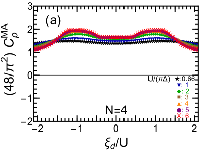
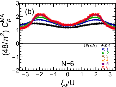
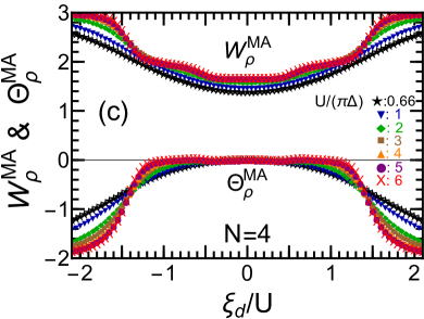
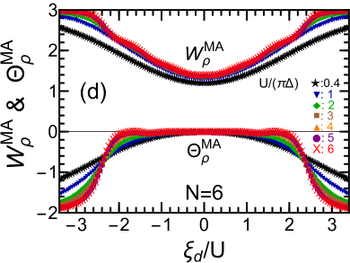
Figure 11: $\xi_{d}$ dependence of $C_{\varrho}^{\mathrm{MA}}=(\pi^{2}/48)(W_{\varrho}^{\mathrm{MA}}+\Theta_{\varrho}^{\mathrm{MA}})$, two-body part $W_{\varrho}^{\mathrm{MA}}$, and three-body part $\Theta_{\varrho}^{\mathrm{MA}}=\Theta_{\mathrm{I}}+\widetilde{\Theta}_{\mathrm{II}}$. Left panels: $N=4$, for $U/(\pi\Delta)=2/3(\star)$, $1(\blacktriangledown)$, $2(\blacklozenge)$, $3(\blacksquare)$, $4(\blacktriangle)$, $5(\bullet)$, $6(\times)$. Right panels: $N=6$, for $U/(\pi\Delta)=2/5(\star)$, $1(\blacktriangledown)$, $2(\blacklozenge)$, $3(\blacksquare)$, $4(\blacktriangle)$, $5(\bullet)$, $6(\times)$.

X.2 $C_{\kappa}^{\mathrm{MA}}$: order $T^{3}$ term of $\kappa_{\mathrm{MA}}$

We next consider the order $T^{3}$ term of thermal conductivity $\kappa_{\mathrm{MA}}$ of the SU($N$) symmetric magnetic alloys. The coefficient $C_{\kappa}^{\mathrm{MA}}$, defined in tables 1 and 2, consists of two-body $W_{\kappa}^{\mathrm{MA}}$ and three-body $\Theta_{\kappa}^{\mathrm{MA}}$ parts:

$$C_{\kappa}^{\mathrm{MA}}\,=\,\frac{\pi^{2}}{64}\,\bigl{(}W_{\kappa}^{\mathrm{MA}}+\Theta_{\kappa}^{\mathrm{MA}}\bigr{)},\qquad\Theta_{\mathrm{\kappa}}^{\mathrm{MA}}\,\equiv\,\Theta_{\mathrm{I}}+\frac{5}{21}\widetilde{\Theta}_{\mathrm{II}}.$$ (90)

Note that $\Theta_{\mathrm{\kappa}}^{\mathrm{MA}}\equiv\Theta_{\mathrm{\kappa}}^{\mathrm{QD}}$, i.e., the three-body part for $C_{\kappa}^{\mathrm{MA}}$ of magnetic alloys is identical to the one for the $T^{3}$ thermal conductance of quantum dots. The NRG results for these coefficients $C_{\kappa}^{\mathrm{MA}}$, $W_{\kappa}^{\mathrm{MA}}$, and $\Theta_{\kappa}^{\mathrm{MA}}$ are shown in Figs. 12(a)–12(d) for $N=4$ and $6$.

The coefficient $C_{\kappa}^{\mathrm{MA}}$ for magnetic alloys is less sensitive to $\xi_{d}$ as compared to $C_{\kappa}^{\mathrm{QD}}$ for for quantum dots. This difference is causes by the contribution of the first term, $(11\pi^{2}/60)\cos^{2}\delta$, in the right-hand side of Eq. (85). The coefficient $C_{\kappa}^{\mathrm{MA}}$ is positive and has a broad peak at $\xi_{d}=0$, the height of which is determined by the two-body contribution $W_{\kappa}^{\mathrm{MA}}$ as three-body part $\Theta_{\kappa}^{\mathrm{MA}}$ vanishes in the electron-hole symmetric case:

$$W_{\kappa}^{\mathrm{MA}}\,\xrightarrow{\,\xi_{d}=0}\,1+\frac{6\widetilde{K}^{2}}{7(N-1)}\,,\qquad\Theta_{\kappa}^{\mathrm{MA}}\xrightarrow{\,\xi_{d}=0\,}0\,.$$ (91)

In the limit of $U\to\infty$, it reaches the maximum possible value $[80/(7\pi^{2})]C_{\kappa}^{\mathrm{MA}}\xrightarrow{\,\xi_{d}=0\,\&\,U\to\infty}9/7$ and $41/35$ for $N=4$ and $6$, respectively.

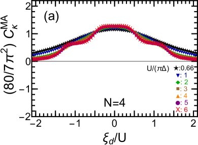
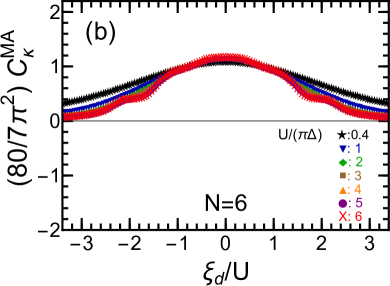
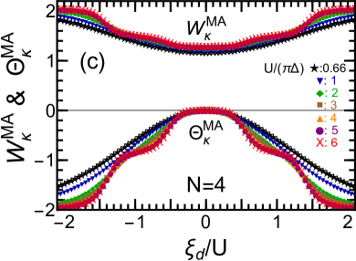
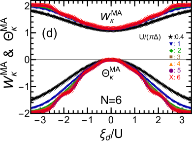
Figure 12: $\xi_{d}$ dependence of $C_{\kappa}^{\mathrm{MA}}=(7\pi^{2}/80)(W_{\kappa}^{\mathrm{MA}}+\Theta_{\kappa}^{\mathrm{MA}})$, two-body part $W_{\kappa}^{\mathrm{MA}}$, and three-body part $\Theta_{\kappa}^{\mathrm{MA}}=\Theta_{\mathrm{I}}+\frac{5}{21}\widetilde{\Theta}_{\mathrm{II}}$. Left panels: $N=4$, for $U/(\pi\Delta)=2/3(\star)$, $1(\blacktriangledown)$, $2(\blacklozenge)$, $3(\blacksquare)$, $4(\blacktriangle)$, $5(\bullet)$, $6(\times)$. Right panels: $N=6$, for $U/(\pi\Delta)=2/5(\star)$, $1(\blacktriangledown)$, $2(\blacklozenge)$, $3(\blacksquare)$, $4(\blacktriangle)$, $5(\bullet)$, $6(\times)$.

In the strong-coupling region $|\xi_{d}|\lesssim(N-1)U/2$, the coefficient $C_{\kappa}^{\mathrm{MA}}$ takes the following form for large $U$,

$$C_{\kappa}^{\mathrm{MA}}\,\simeq\,\frac{\pi^{2}}{240}\left[32+\left(11-\frac{18}{N-1}\right)\,\cos 2\delta\,+\,16\,\Theta_{\mathrm{I}}\right].$$ (92)

This is because, in this region, the rescaled Wilson ratio is almost saturated $\widetilde{K}\simeq 1$ (see Appendix D) and the three-body part is parameterized by a single component, $\Theta_{\kappa}^{\mathrm{MA}}\simeq\frac{16}{21}\,\Theta_{\mathrm{I}}$, due to the property described in Eq. (61). The plateau structures of $C_{\kappa}^{\mathrm{MA}}$, appearing in Figs. 12(a) and 12(b) around the integer filling points $N_{d}=1$, $2$, $\ldots$, $N-1$, are determined by both the $\cos 2\delta$ term in $W_{\kappa}^{\mathrm{MA}}$ and the plateaus occurring in $\Theta_{\kappa}^{\mathrm{MA}}$ seen in Figs. 12(c) and 12(d).

In contrast, at $|\xi_{d}|\gtrsim(N-1)U/2$, the electron filling approaches the empty $N_{d}\simeq 0$ or the fully occupied $N_{d}\simeq N$ states as the impurity level goes very far away from the half filled point. Therefore, the order $T^{3}$ thermal conductivity for magnetic alloys also approaches the noninteracting value in this limit:

$$W_{\kappa}^{\mathrm{MA}}\,\xrightarrow{\,|\xi_{d}|\to\infty}\,\frac{43}{21},\qquad\Theta_{\kappa}^{\mathrm{MA}}\,\xrightarrow{\,|\xi_{d}|\to\infty}\,-2,$$ (93)

and thus $[80/(7\pi^{2})]\,C_{\kappa}^{\mathrm{MA}}\,\xrightarrow{\,|\xi_{d}|\to\infty}1/21$.

X.3 $C_{L}^{\mathrm{MA}}$: order $T^{2}$ term of $L_{\mathrm{MA}}$

The Lorenz number $L_{\mathrm{MA}}\equiv\kappa_{\mathrm{MA}}/(\sigma_{\mathrm{MA}}\,T)$ for magnetic alloys is defined as the ration of the thermal conductivity $\kappa_{\mathrm{MA}}/T$ to electrical conductivity $\sigma_{\mathrm{MA}}$. It takes the universal Wiedemann-Franz value at zero temperature: $L_{\mathrm{MA}}\xrightarrow{T\to 0}\pi^{2}/(3e^{2})$. However, it deviates from this value as the temperature increases, showing the $T^{2}$ dependence described in Eq. (83). The precise expansion formula for the coefficient $C_{L}^{\mathrm{MA}}$ for the order $T^{2}$ term is shown in table 2. It is given by the difference $C_{L}^{\mathrm{MA}}=C_{\varrho}^{\mathrm{MA}}-C_{\kappa}^{\mathrm{MA}}$ between the order $T^{2}$ term of the resistivities $1/\sigma_{\mathrm{MA}}$ and $T/\kappa_{\mathrm{MA}}$, defined by Eqs. (81) and (83). The coefficient $C_{L}^{\mathrm{MA}}$ for magnetic alloys and the quantum-dot counterpart $C_{L}^{\mathrm{QM}}$ are related to each other through Eq. (86): these two coefficients tend to have opposite signs. In Appendix G, we have also provide an analytic formula for $C_{L}^{\mathrm{MA}}$ in the noninteraction case, for comparison.

The NRG results for $C_{L}^{\mathrm{MA}}$ are shown in Figs. 13(a) and 13(b) for $N=4$ and $6$, respectively. Near half filling $|\xi_{d}|\lesssim U/2$, the coefficient $C_{L}^{\mathrm{MA}}$ is determined by the two-body part $W_{L}^{\mathrm{MA}}$ as the three-body part, given by $-16\Theta_{\mathrm{I}}$, vanishes at $\xi_{d}=0$:

$$C_{L}^{\mathrm{MA}}\,\xrightarrow{\,\xi_{d}=0}\,-\frac{\pi^{2}}{30}\left(2+\frac{\widetilde{K}^{2}}{N-1}\right)\ <0\,.$$ (94)

This coefficient takes the greatest possible negative value, $C_{L}^{\mathrm{MA}}\xrightarrow{\xi_{d}=0\,\&\,U=\infty}-0,767\cdots$ for $N=4$, and $-0.723\cdots$ for $N=6$, in the limit of $U\to\infty$ where $\widetilde{K}\to 1$.

In the strong-coupling region $|\xi_{d}|\lesssim(N-1)U/2$, the $C_{L}^{\mathrm{MA}}$ also exhibits the plateau structures around the integer filling points $\xi_{d}/U=0$, $\pm 1$, $\ldots$, $\pm(N-2)/2$ for large $U$, reflecting the structures that appear for both $C_{\varrho}^{\mathrm{MA}}$ and $C_{\kappa}^{\mathrm{MA}}$. In particular, the plateaus at $N_{d}\simeq\frac{N}{2}\pm 1$ fillings, seen in Figs. 13(a) and 13(b) for $U/(\pi\Delta)\gtrsim 3$, take a negative value for both $N=4$ and $N=6$, whereas the other plateaus become positive for $N=6$ as the electrical resistivity dominates, i.e., $C_{\varrho}^{\mathrm{MA}}>C_{\kappa}^{\mathrm{MA}}$.

As the impurity level goes far away from the Fermi level in the region $|\xi_{d}|\gtrsim(N-1)U/2$, the occupation number approaches $N_{d}\simeq 0$ or $N_{d}\simeq N$. In the limit of $|\xi_{d}|\to\infty$, the two-body and three-body parts take the noninteracting values, $W_{L}^{\mathrm{MA}}\xrightarrow{|\xi_{d}|\to\infty}-28$ and $-16\Theta_{\mathrm{I}}\xrightarrow{|\xi_{d}|\to\infty}32$, and the coefficient $C_{L}^{\mathrm{MA}}$ converges to the positive value,

$$C_{L}^{\mathrm{MA}}\,\xrightarrow{\,|\xi_{d}|\to\infty}\,\frac{\pi^{2}}{60}\ =\ 0.164\cdots\ >0\,.$$ (95)

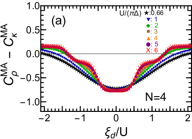
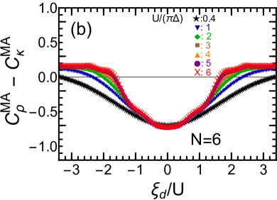
Figure 13: Order $T^{2}$ term $C_{L}^{\mathrm{MA}}=C_{\varrho}^{\mathrm{MA}}-C_{\kappa}^{\mathrm{MA}}$ of Lorenz number $L_{\mathrm{MA}}$ is plotted vs $\xi_{d}$. Left panel: $N=4$, for $U/(\pi\Delta)=2/3(\star)$, $1(\blacktriangledown)$, $2(\blacklozenge)$, $3(\blacksquare)$, $4(\blacktriangle)$, $5(\bullet)$, $6(\times)$. Right panel: $N=6$, for $U/(\pi\Delta)=2/5(\star)$, $1(\blacktriangledown)$, $2(\blacklozenge)$, $3(\blacksquare)$, $4(\blacktriangle)$, $5(\bullet)$, $6(\times)$.

XI Summary

We have presented a comprehensive Fermi-liquid description for nonlinear current and thermoelectric transport through quantum dots and magnetic alloys, which is asymptotically exact at low energies up to the next-leading order terms. Our formulation is based on the multilevel Anderson model and is applicable to arbitrary impurity-level structures $\epsilon_{d\sigma}$ for $\sigma=1$, $2$, $\ldots$, $N$, including the spin degrees of freedom. The coefficients for the next-leading order terms have been shown to be expressed in terms of a set of the correlation functions defined with respect to the equilibrium ground state: the phase shift $\delta_{\sigma}$, the static susceptibilities $\chi_{\sigma_{1},\sigma_{2}}$, and the three-body correlations $\chi_{\sigma_{1},\sigma_{2},\sigma_{3}}^{[3]}$ which emerge when the system does not have both the electron-hole and time-reversal symmetries.

Extending Yamada-Yosida’s field theoretical approach, we have obtained the formulas for the differential conductance $dI/dV$, current noise $S_{\mathrm{noise}}^{\mathrm{QD}}$ and thermal conductance $\kappa_{\mathrm{QD}}$ of quantum dots, and also the electrical resistivity $\varrho_{\mathrm{MA}}$ and thermal conductivity $\kappa_{\mathrm{MA}}$ of dilute magnetic alloys. In the SU($N$) symmetric case, these transport coefficients take simplified forms, as listed in tables 1 and 2, and the three-body correlations can be deduced from the derivatives of the susceptibilities: $\partial\overline{\chi}_{C}/\partial\epsilon_{d}$, $\partial\overline{\chi}_{S}/\partial\epsilon_{d}$, and $\chi_{B}^{[3]}$ through Eqs.  (42)–(45).

We have also calculated the correlation functions for the SU(4) and SU(6) cases, using the NRG approach over a whole region of impurity-electron fillings $N_{d}$, which includes the Kondo and the valence-fluctuation regimes. In the SU($N$) case, the three-body correlations have three linearly independent components that approach each other closely as the Coulomb interaction $U$ increases: $\chi_{\sigma\sigma\sigma}^{[3]}\simeq-(N-1)\chi_{\sigma\sigma^{\prime}\sigma^{\prime}}^{[3]}\simeq\frac{(N-1)(N-2)}{2}\chi_{\sigma\sigma^{\prime}\sigma^{\prime\prime}}^{[3]}$ for $\sigma\neq\sigma^{\prime}\neq\sigma^{\prime\prime}\neq\sigma$, in a wide filling range $1\lesssim N_{d}\lesssim N-1$. This is caused by the suppression of the derivatives of the charge and spin susceptibilities, occurring at large $U$: $|\partial\overline{\chi}_{C}/\partial\epsilon_{d}|\ll(T^{*})^{-2}$ and $|\partial\overline{\chi}_{S}/\partial\epsilon_{d}|\ll(T^{*})^{-2}$, with $T^{*}\equiv 1/(4\chi_{\sigma\sigma})$ the characteristic energy scale of SU($N$) Fermi liquid. This property of three-body correlations is also related to a similar property of linear susceptibilities, $\chi_{\sigma\sigma}\simeq-(N-1)\chi_{\sigma\sigma^{\prime}}$, which reflects the suppression of charge fluctuations, $\overline{\chi}_{C}\simeq 0$, occurring at large $U$.

The coefficients $C$’s for the next-leading order terms can be decomposed into the two-body part $W$’s and the three-body part $\Theta$’s, as listed in table 2. The NRG results show that the three-body part $\Theta_{V}$ of the coefficient $C_{V}$ for the order $(eV)^{2}$ term of $dI/dV$ exhibits the Kondo plateau structures at integer filling points $N_{d}=1$, $2$, $\ldots$, $N-1$ for large $U$. These plateaus of $\Theta_{V}$ complement the two body part $W_{V}$ that decreases away from half filling to form a wide ridge structure in $C_{V}$, which spreads over the region of $1\lesssim N_{d}\lesssim N-1$.

The linear-response term of current noise $S_{\mathrm{noise}}^{\mathrm{QD}}$ is maximized at quarter filling $N_{d}/N=1/4$ and three-quarters $3/4$ filling, and the peaks exhibit flat structures for $N=4$, while they are round for $N=6$. This difference is caused by the fact that, at these fillings, the SU($N$) Kondo effects occur for $N\equiv 0$ (mod $4$), while the intermediate valence fluctuations occur for $N\equiv 2$ (mod $4$). The coefficient $C_{S}$ for the order $|eV|^{3}$ nonlinear term of $S_{\mathrm{noise}}^{\mathrm{QD}}$ has a peak at half filling, which evolves into a plateau as $U$ increases. As the impurity level $\xi_{d}$ deviates from the half filling point, $C_{S}$ decreases rapidly for $N=4$, whereas it varies more modestly for $N=6$. This is mainly due to the higher-harmonic “$\sin 4\delta$” dependence of the three-body part $\Theta_{S}$, which vanishes at the quarter and three-quarters filling points. As $|\xi_{d}|$ increases further, $\Theta_{S}$ has a pronounced negative minimum in the valence fluctuation regions at $\xi_{d}\simeq\pm(N-1)U/2$ for both $N=4$ and $6$, which yield the valley structures appearing in $C_{S}$. This is in marked contrast to the SU(2) case, where the valley structure emerging in $C_{S}$ is caused by the two-body contributions $W_{S}$, instead of $\Theta_{S}$.

We have also studied the coefficient $C_{T}$ for the order $T^{2}$ term of linear conductance $g\equiv\left.dJ/dV\right|_{eV=0}$ and the coefficient $C_{\kappa}^{\mathrm{QD}}$ for the order $T^{3}$ term of thermal conductance $\kappa_{\mathrm{QD}}$, for SU($N$) quantum dots. The three-body part $\Theta_{T}$ of $C_{T}$ is determined solely by the derivatives of charge and spin susceptibilities, i.e., $\partial\overline{\chi}_{C}/\partial\epsilon_{d}$ and $\partial\overline{\chi}_{S}/\partial\epsilon_{d}$, and is independent of $\chi_{B}^{[3]}$. Therefore, $\Theta_{T}$ is significantly suppressed and almost vanishes for strong interactions $U$ in a wide range of the electron filling $1\lesssim N_{d}\lesssim N-1$. In contrast, the three-body part $\Theta_{\kappa}^{\mathrm{QD}}$ for thermal conductance involves $\chi_{B}^{[3]}$ and becomes comparable to the two-body part $W_{\kappa}^{\mathrm{QD}}$, except for the plateau region near half filling. The Lorenz number $L_{\mathrm{QD}}\equiv\kappa_{\mathrm{QD}}/(g\,T)$ for quantum dots takes the universal Wiedemann-Franz value $\pi^{2}/(3e^{2})$ at $T=0$, and shows the $T^{2}$ dependence at low temperatures. The coefficient for the order $T^{2}$ term of $L_{\mathrm{QD}}$ is given by $C_{L}^{\mathrm{QD}}=C_{\kappa}^{\mathrm{QD}}-C_{T}$, i.e., the difference between the next-leading order terms of $\kappa_{\mathrm{QD}}$ and $g$. This coefficient $C_{L}^{\mathrm{QD}}$ also exhibits the Kondo plateau structures at integer filling points $N_{d}=1$, $2$, $\ldots$, $N-1$.

The three-body correlations also play a significant role in the low-energy transport of magnetic alloys. We have investigated the behaviors of the coefficient $C_{\varrho}^{\mathrm{MA}}$ for the order $T^{2}$ resistivity $\varrho_{\mathrm{MA}}$ and $C_{\kappa}^{\mathrm{MA}}$ for the order $T^{3}$ thermal conductivity $\kappa_{\mathrm{MA}}$. In the SU($N$) symmetric case, the three-body parts of these coefficients become identical to the related ones for quantum dots, i.e., $\Theta_{\varrho}^{\mathrm{MA}}\equiv\Theta_{T}$ and $\Theta_{\kappa}^{\mathrm{MA}}\equiv\Theta_{\kappa}^{\mathrm{QD}}$. Therefore, the difference between the coefficients for MA and that for the QD counterparts arises from the two-body parts, more specifically, from the additional $\cos^{2}\delta$ terms appearing in the right-hand side of Eqs. (84) and (85). The additional $\cos^{2}\delta$ terms make the coefficients $C_{\varrho}^{\mathrm{MA}}$ and $C_{\kappa}^{\mathrm{MA}}$ positive definite and less sensitive to the impurity level position $\xi_{d}$, compared to the QD counterparts $C_{T}$ and $C_{\kappa}^{\mathrm{QD}}$. The coefficient $C_{\varrho}^{\mathrm{MA}}$ takes the maximum value at the electron fillings of $N_{d}\simeq 1$ and $N-1$ for $N\geq 4$, while in the SU(2) case $C_{\varrho}^{\mathrm{MA}}$ has a single peak at half filling. The coefficient $C_{L}^{\mathrm{MA}}=C_{\varrho}^{\mathrm{MA}}-C_{\kappa}^{\mathrm{MA}}$ for the order $T^{2}$ term of the Lorenz number $L_{\mathrm{MA}}\equiv\kappa_{\mathrm{MA}}/(\sigma_{\mathrm{MA}}\,T)$ for magnetic alloys also becomes less sensitive to the electron filling $N_{d}$, compared to $C_{L}^{\mathrm{QD}}$ for quantum dots.

The three-body correlation functions can be determined experimentally by measuring the coefficients $C$’s for the next leading order terms. These experimental values can then be used to infer the behaviors of other unmeasured transport coefficients.

Appendix A Fermi-liquid parameters

A.1 Linear and nonlinear static susceptibilities

The ground-state properties and the leading Fermi-liquid corrections due to the low-lying excitations can be described in terms of the occupation number and the linear susceptibilities of the impurity level, derived from the free energy $\Omega\equiv-(1/\beta)\,\log\,\bigl{[}\,\mathrm{Tr}\,e^{-\beta H}\,\bigr{]}$:

$$\bigl{\langle}n_{d\sigma}\bigr{\rangle}\,= \ \frac{\partial\Omega}{\partial\epsilon_{d\sigma}}\,,$$ (96)

$$\chi_{\sigma\sigma^{\prime}}\,\equiv \ -\frac{\partial^{2}\Omega}{\partial\epsilon_{d\sigma}\partial\epsilon_{d\sigma^{\prime}}}\,=\,\int_{0}^{\beta}\!d\tau\,\bigl{\langle}\delta n_{d\sigma}(\tau)\,\delta n_{d\sigma^{\prime}}\bigr{\rangle}\,.$$ (97)

Here, $\delta n_{d\sigma}\equiv n_{d\sigma}-\langle n_{d\sigma}\rangle$, and thermal-equilibrium averages are defined as $\langle O\rangle=\mathrm{Tr}\,\bigl{[}\,e^{-\beta\mathcal{H}}\,\mathcal{O}\,\bigr{]}/\mathrm{Tr}\,e^{-\beta\mathcal{H}}$, with $\beta=1/T$ the inverse temperature.

In addition to the linear susceptibilities, the nonlinear ones $\chi_{\sigma_{1}\sigma_{2}\sigma_{3}}^{[3]}$ are essential to the next-leading-order corrections when the system does not have both the electron-hole and time-reversal symmetries:

$$\chi_{\sigma_{1}\sigma_{2}\sigma_{3}}^{[3]}\,\equiv\,-\frac{\partial^{3}\Omega}{\partial\epsilon_{d\sigma_{1}}\partial\epsilon_{d\sigma_{2}}\partial\epsilon_{d\sigma_{3}}}\,=\,\frac{\partial\chi_{\sigma_{1}\sigma_{2}}}{\partial\epsilon_{d\sigma_{3}}}$$

$$= -\int_{0}^{\beta}\!d\tau_{1}\!\int_{0}^{\beta}\!d\tau_{2}\,\bigl{\langle}T_{\tau}\delta n_{d\sigma_{1}}(\tau_{1})\,\delta n_{d\sigma_{2}}(\tau_{2})\,\delta n_{d\sigma_{3}}\bigr{\rangle}\,.$$ (98)

Here, $T_{\tau}$ is the imaginary-time ordering operator. This correlation function has the permutation symmetry: $\chi_{\sigma_{1}\sigma_{2}\sigma_{3}}^{[3]}=\chi_{\sigma_{2}\sigma_{1}\sigma_{3}}^{[3]}=\chi_{\sigma_{3}\sigma_{2}\sigma_{1}}^{[3]}=\chi_{\sigma_{1}\sigma_{3}\sigma_{2}}^{[3]}=\cdots.$ Specifically, in our formulation we are using the ground state values for $\langle n_{d\sigma}\rangle$, $\chi_{\sigma\sigma^{\prime}}$ and $\chi_{\sigma_{1}\sigma_{2}\sigma_{3}}^{[3]}$, determined at $T=0$.

The occupation number can be related to the phase shift through the Friedel sum rule: $\langle n_{d\sigma}\rangle\xrightarrow{\,T=eV=0\,}\delta_{\sigma}/\pi$, with $\delta_{\sigma}$ defined as the argument of the complex value of Green’s function at $\omega=T=eV=0$, as $G_{\sigma}^{r}(0)=-\left|G_{\sigma}^{r}(0)\right|e^{i\delta_{\sigma}}$.Shiba (1975) Conversely, the value of the spectral function $\rho_{d\sigma}(\omega)$ at $\omega=0$ can be expressed in terms of the phase shift, as

$$\rho_{d\sigma}\,\equiv\,\rho_{d\sigma}(0)\,=\,\frac{\sin^{2}\delta_{\sigma}}{\pi\Delta}\,.$$ (99)

Note that the $\omega$-dependent $\rho_{d\sigma}(\omega)$ is defined with respect to the equilibrium ground state, as

$$\rho_{d\sigma}(\omega)\,\equiv\,A_{\sigma}(\omega)\Big{|}_{T=eV=0}\,,$$ (100)

with $A_{\sigma}(\omega)$ given in Eq. (9).

The derivative of $\rho_{d\sigma}(\omega)$ also plays an important role in the next-leading-order corrections and can be expressed in terms of the diagonal susceptibility $\chi_{\sigma\sigma}$, using Eq. (106), as

$$\rho_{d\sigma}^{\prime}\equiv\left.\frac{\partial\rho_{d\sigma}(\omega)}{\partial\omega}\right|_{\omega=0}=\,-\frac{\partial\rho_{d\sigma}}{\partial\epsilon_{d\sigma}}\ =\ \frac{\chi_{\sigma\sigma}}{\Delta}\,\sin 2\delta_{\sigma}.$$ (101)

One of the most typical Fermi-liquid corrections due to the many-body scatterings emerges in the $T$-linear specific heat $\mathcal{C}_{\mathrm{imp}}^{\mathrm{heat}}$ of the impurity electrons:

$$\mathcal{C}_{\mathrm{imp}}^{\mathrm{heat}}\,=\,\gamma_{\mathrm{imp}}\,T\,,\qquad\gamma_{\mathrm{imp}}\,\equiv\,\frac{\pi^{2}}{3}\sum_{\sigma}\chi_{\sigma\sigma}\,.$$ (102)

The coefficient $\gamma_{\mathrm{imp}}$ can be expressed in terms of the diagonal components of the linear susceptibility $\chi_{\sigma\sigma}$ using the Ward identitiesYamada (1975a); Shiba (1975); Yoshimori (1976), which follow from the relationship between the derivative of the self-energy with respect to $\omega$ and the derivative with respect to $\epsilon_{d\sigma^{\prime}}$, described briefly in the following.

A.2 Ward identities

The local Fermi-liquid state of the quantum impurity systems can microscopically be described using the retarded Green’s function, defined in Eq. (8), which can also be written in the form,

$$G_{\sigma}^{r}(\omega)\,= \ \frac{1}{\omega-\epsilon_{d\sigma}+i\Delta-\Sigma_{\sigma}^{r}(\omega)}\,.$$ (103)

The information about the low-lying energy states can be extracted from the equilibrium self-energy $\Sigma_{\mathrm{eq},\sigma}^{r}(\omega)\equiv\left.\Sigma_{\sigma}^{r}(\omega)\right|_{T=eV=0}$, by expanding it, step by step, around the Fermi energy $\omega=0$. The expansion up to the $\omega$-linear terms describes the renormalized resonance state of the form,

$$G_{\sigma}^{r}(\omega)\,\simeq \ \frac{z_{\sigma}}{\omega-\widetilde{\epsilon}_{d\sigma}+i\widetilde{\Delta}_{\sigma}}\,.$$ (104)

Here, the renormalized parameters are defined by

$$\widetilde{\epsilon}_{d\sigma}\,\equiv \ z_{\sigma}\left[\epsilon_{d\sigma}+\Sigma_{\mathrm{eq},\sigma}^{r}(0)\right]\,=\,\widetilde{\Delta}_{\sigma}\cot\delta_{\sigma}\,,$$

$$\widetilde{\Delta}_{\sigma}\,\equiv \ z_{\sigma}\Delta,\qquad\frac{1}{z_{\sigma}}\,\equiv\ 1-\left.\frac{\partial\Sigma_{\mathrm{eq},\sigma}^{r}(\omega)}{\partial\omega}\right|_{\omega=0}.\rule{0.0pt}{17.07182pt}$$ (105)

The wavefunction renormalization factor $z_{\sigma}$ can be related to the derivative of $\Sigma_{\mathrm{eq},\sigma}^{r}(0)$ with respect to the impurity level $\epsilon_{d\sigma^{\prime}}$, using the Ward identity:Yamada (1975a); Shiba (1975); Yoshimori (1976)

$$\frac{1}{z_{\sigma}}\,=\,\widetilde{\chi}_{\sigma\sigma}\,,\qquad\quad\widetilde{\chi}_{\sigma\sigma^{\prime}}\,\equiv\,\delta_{\sigma\sigma^{\prime}}+\frac{\partial\Sigma_{\mathrm{eq},\sigma}^{r}(0)}{\partial\epsilon_{d\sigma^{\prime}}}\,.$$ (106)

The coefficient $\widetilde{\chi}_{\sigma\sigma^{\prime}}$ determines the extent to which the susceptibility is enhanced at $T=0$:

$$\chi_{\sigma\sigma^{\prime}}\,=\,-\frac{\partial\bigl{\langle}n_{d\sigma}\bigr{\rangle}}{\partial\epsilon_{d\sigma^{\prime}}}\ \xrightarrow{\,T\to 0\,}\ \rho_{d\sigma}\widetilde{\chi}_{\sigma\sigma^{\prime}}\,.$$ (107)

It has recently been clarified that the order $\omega^{2}$ real part of the self-energy can be expressed in terms of the the diagonal component of the three-body correlation function $\chi_{\sigma\sigma\sigma}^{[3]}$, as Filippone et al. (2017); Oguri and Hewson (2018a, b, c)

$$\!\!\!\left.\frac{\partial^{2}}{\partial\omega^{2}}\mathrm{Re}\,\Sigma_{\mathrm{eq},\sigma}^{r}(\omega)\right|_{\omega\to 0}\,=\,\frac{\partial^{2}\Sigma_{\mathrm{eq},\sigma}^{r}(0)}{\partial\epsilon_{d\sigma}^{2}}\,\ \ =\ \frac{\partial\widetilde{\chi}_{\sigma\sigma}}{\partial\epsilon_{d\sigma}}\,.$$ (108)

Physically, this coefficient determines the energy shifts of quasiparticles of order $\omega^{2}$, $T^{2}$ and $(eV)^{2}$, which affect the low-energy transport of the next-leading order.

Appendix B Low-energy asymptotic form of spectral function

The low-energy asymptotic form of the retarded self-energy $\Sigma_{\sigma}^{r}(\omega)$ for multilevel Anderson impurity model has been derived up to terms of order $\omega^{2}$, $T^{2}$, and $(eV)^{2}$ in the previous works.Oguri et al. (2022); Tsutsumi et al. (2023) For symmetric tunnel junctions with $\Gamma_{L}=\Gamma_{R}$ ($=\Delta/2$) and $\mu_{L}=-\mu_{R}$ ($=eV/2$), it takes the form,

$$\mathrm{Im}\,\Sigma_{\sigma}^{r}(\omega)\,= \ -\,\frac{\pi}{2}\,\frac{1}{\rho_{d\sigma}}\sum_{\sigma^{\prime}(\neq\sigma)}\chi_{\sigma\sigma^{\prime}}^{2}\,\left[\,\omega^{2}+\frac{3}{4}\,(eV)^{2}+(\pi T)^{2}\,\right]\ +\,\cdots\,,$$ (109)

$$\epsilon_{d\sigma}+\mathrm{Re}\,\Sigma_{\sigma}^{r}(\omega)\,= \ \ \Delta\,\cot\delta_{\sigma}\,+\bigl{(}1-\widetilde{\chi}_{\sigma\sigma}\bigr{)}\,\omega\,+\frac{1}{2}\,\frac{\partial\widetilde{\chi}_{\sigma\sigma}}{\partial\epsilon_{d\sigma}}\,\omega^{2}\,+\frac{1}{6}\,\frac{1}{\rho_{d\sigma}}\sum_{\sigma^{\prime}(\neq\sigma)}\chi_{\sigma\sigma^{\prime}\sigma^{\prime}}^{[3]}\left[\frac{3}{4}\,(eV)^{2}+\left(\pi T\right)^{2}\right]\ +\,\cdots$$ (110)

Substituting these expansion results into Eq. (103), we obtain the asymptotic form spectral function,

$$\pi\Delta\,A_{\sigma}(\omega)\,= \ \sin^{2}\delta_{\sigma}+\frac{\pi^{2}}{3}\left(\frac{3}{2}\cos 2\delta_{\sigma}\,\sum_{\sigma^{\prime}(\neq\sigma)}\chi_{\sigma\sigma^{\prime}}^{2}-\frac{\sin 2\delta_{\sigma}}{2\pi}\,\sum_{\sigma^{\prime}(\neq\sigma)}\chi_{\sigma\sigma^{\prime}\sigma^{\prime}}^{[3]}\,\right)\left[\,\frac{3}{4}\left(eV\right)^{2}+\left(\pi T\right)^{2}\,\right]$$

$$\ +\pi\sin 2\delta_{\sigma}\,\chi_{\sigma\sigma}\,\omega+\pi^{2}\left[\,\cos 2\delta_{\sigma}\left(\chi_{\sigma\sigma}^{2}+\frac{1}{2}\sum_{\sigma^{\prime}(\neq\sigma)}\chi_{\sigma\sigma^{\prime}}^{2}\right)-\frac{\sin 2\delta_{\sigma}}{2\pi}\,\chi_{\sigma\sigma\sigma}^{[3]}\,\right]\,\omega^{2}\ +\ \cdots.$$ (111)

Correspondingly, the inverse of the spectral function that determines the thermoelectric transport of magnetic alloys takes the following form, up to terms order $\omega^{2}$ and $T^{2}$ at $eV=0$,

$$\frac{1}{\pi\Delta A_{\sigma}(\omega)}\,\simeq \ \frac{1}{\pi\Delta\rho_{d\sigma}}\Biggl{[}1-\frac{1}{6\Delta\rho_{d\sigma}}\left(\,3\pi\cos 2\delta_{\sigma}\sum_{\sigma^{\prime}(\neq\sigma)}\chi_{\sigma\sigma^{\prime}}^{2}-\sin 2\delta_{\sigma}\,\sum_{\sigma^{\prime}(\neq\sigma)}\chi_{\sigma\sigma^{\prime}\sigma^{\prime}}^{[3]}\,\right)\left(\pi T\right)^{2}-\frac{\sin 2\delta_{\sigma}\,\chi_{\sigma\sigma}}{\Delta\rho_{d\sigma}}\,\omega$$

$$\qquad\qquad+\frac{\pi}{\Delta\rho_{d\sigma}}\left\{\,\left(\cos 2\delta_{\sigma}+2\right)\,\chi_{\sigma\sigma}^{2}-\frac{1}{2}\cos 2\delta_{\sigma}\sum_{\sigma^{\prime}(\neq\sigma)}\chi_{\sigma\sigma^{\prime}}^{2}+\frac{\sin 2\delta_{\sigma}}{2\pi}\,\chi_{\sigma\sigma\sigma}^{[3]}\,\right\}\,\omega^{2}\Biggr{]}+\cdots\;.$$ (112)

Appendix C Properties of $\chi_{\sigma_{1}\sigma_{2}\sigma_{3}}^{[3]}$ in SU($N$) case

We briefly describe here some relations between the three-body correlation functions and the derivative of the linear susceptibilities with respect to the center of mass coordinate of the impurity levels, $\epsilon_{d}\equiv(1/N)\sum_{\sigma}\epsilon_{d\sigma}$.

The derivative of the diagonal susceptibility $\chi_{\sigma\sigma}$ can be written as

$$\frac{\partial\chi_{\sigma\sigma}}{\partial\epsilon_{d}} =\ \frac{\partial\chi_{\sigma\sigma}}{\partial\epsilon_{d\sigma}}+\sum_{\sigma^{\prime}(\neq\sigma)}\frac{\partial\chi_{\sigma\sigma}}{\partial\epsilon_{d\sigma^{\prime}}}$$

$$\xrightarrow{\,\mathrm{SU}(N)\,}\,\chi_{\sigma\sigma\sigma}^{[3]}+(N-1)\,\chi_{\sigma\sigma^{\prime}\sigma^{\prime}}^{[3]}\,,$$ (113)

where $\sigma\neq\sigma^{\prime}$. Note that $\chi_{\sigma\sigma\sigma^{\prime}}^{[3]}=\chi_{\sigma\sigma^{\prime}\sigma^{\prime}}^{[3]}$ in the SU($N$) symmetric case. Similarly, the derivative of the off-diagonal susceptibility $\chi_{\sigma\sigma^{\prime}}$ for $\sigma\neq\sigma^{\prime}$ takes the form

$$\frac{\partial\chi_{\sigma\sigma^{\prime}}}{\partial\epsilon_{d}}= \ \frac{\partial\chi_{\sigma\sigma^{\prime}}}{\partial\epsilon_{d\sigma}}+\frac{\partial\chi_{\sigma\sigma^{\prime}}}{\partial\epsilon_{d\sigma^{\prime}}}+\sum_{\sigma^{\prime\prime}(\neq\sigma\atop\neq\sigma^{\prime})}\frac{\partial\chi_{\sigma\sigma^{\prime}}}{\partial\epsilon_{d\sigma^{\prime\prime}}}$$

$$\xrightarrow{\,\mathrm{SU}(N)\,} \ 2\,\chi_{\sigma\sigma^{\prime}\sigma^{\prime}}^{[3]}+(N-2)\,\chi_{\sigma\sigma^{\prime}\sigma^{\prime\prime}}^{[3]}\;,$$ (114)

for $\sigma\neq\sigma^{\prime}\neq\sigma^{\prime\prime}\neq\sigma$. In the SU(2) symmetric case, Eqs. (113) and (114) provide enough information to determine the two independent components $\chi_{\sigma\sigma\sigma}^{[3]}$ and $\chi_{\sigma\sigma^{\prime}\sigma^{\prime}}^{[3]}$ from the two differential coefficients $\partial\chi_{\sigma\sigma}/\partial\epsilon_{d}$ and $\partial\chi_{\sigma\sigma^{\prime}}/\partial\epsilon_{d}$. However, for $N\geq 3$, there are three independent three-body components, i.e., $\chi_{\sigma\sigma\sigma}^{[3]}$, $\chi_{\sigma\sigma^{\prime}\sigma^{\prime}}^{[3]}$, and $\chi_{\sigma\sigma^{\prime}\sigma^{\prime\prime}}^{[3]}$, so that we need additional information to determine all these components.

In order to obtain another independent relation, we consider the derivative of the susceptibilities with respect to the magnetic field $b$, which induces the level splitting in impurity levels $\epsilon_{d\sigma}$ in a such way that $\epsilon_{d,m,\uparrow}=\epsilon_{d}-b$ and $\epsilon_{d,m,\downarrow}=\epsilon_{d}+b$, with $\sigma=(m,s)$ for $m=1,2,\ldots,N/2$ and $s=\uparrow,\downarrow$:

$$\!\!\!\frac{\partial\chi_{m_{1}s_{1},m_{2}s_{2}}}{\partial b}\,=\,\sum_{m_{3}=1}^{N/2}\sum_{s_{3}=\uparrow,\downarrow}\frac{\partial\epsilon_{d,m_{3},s_{3}}}{\partial b}\,\frac{\partial\chi_{m_{1}s_{1},m_{2}s_{2}}}{\partial\epsilon_{d,m_{3},s_{3}}}$$

$$\!\!\!\!=\,-\sum_{m_{3}=1}^{N/2}\,\chi_{m_{1}s_{1},m_{2}s_{2},m_{3}\uparrow}^{[3]}\,+\sum_{m_{3}=1}^{N/2}\chi_{m_{1}s_{1},m_{2}s_{2},m_{3}\downarrow}^{[3]}.$$ (115)

From this derivative, we obtain the following relation, taking $m_{1}=m_{2}\,(\equiv m)$, as

$$\!\!\!\!\!\!\!\!\!\!\!\!\!\!\!\!\!\!\!\!\!\!\!\!\!\!\frac{\partial}{\partial b}\left(\frac{\chi_{m\uparrow,m\uparrow}-\chi_{m\downarrow,m\downarrow}}{2}\right)$$

$$= \ \ -\sum_{m^{\prime}=1}^{N/2}\frac{1}{2}\,\biggl{(}\chi_{m\uparrow,m\uparrow,m^{\prime}\uparrow}^{[3]}-\chi_{m\uparrow,m\uparrow,m^{\prime}\downarrow}^{[3]}$$

$$\qquad\qquad\quad+\chi_{m\downarrow,m\downarrow,m^{\prime}\downarrow}^{[3]}-\chi_{m\downarrow,m\downarrow,m^{\prime}\uparrow}^{[3]}\biggr{)}$$

$$\xrightarrow{\,b\to 0\,} \,-\sum_{m_{3}=1}^{N/2}\left[\,\chi_{m\uparrow,m\uparrow,m_{3}\uparrow}^{[3]}\,-\,\chi_{m\uparrow,m\uparrow,m_{3}\downarrow}^{[3]}\,\right]$$

$$= \ -\left(\chi_{m\uparrow,m\uparrow,m\uparrow}^{[3]}\,-\,\chi_{m\uparrow,m\uparrow,m\downarrow}^{[3]}\right).$$ (116)

Here, we set the magnetic field to be zero, $b=0$, in the last two lines. This relation can also be rewritten into the following form at $b=0$, using the original label $\sigma=(m,s)$, as

$$\chi_{B}^{[3]}\,\equiv\,\frac{\partial}{\partial b}\left(\frac{\chi_{m\uparrow,m\uparrow}-\chi_{m\downarrow,m\downarrow}}{2}\right)_{b=0}=\,-\chi_{\sigma\sigma\sigma}^{[3]}+\chi_{\sigma\sigma^{\prime}\sigma^{\prime}}^{[3]},$$ (117)

for $\sigma^{\prime}\neq\sigma$.

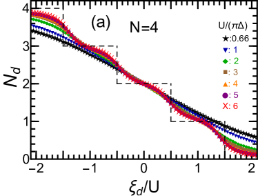
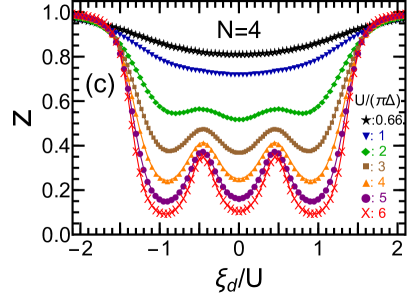
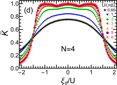
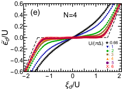
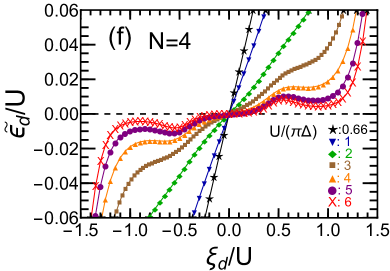
Figure 14: Fermi-liquid parameters for the SU(4) symmetric Anderson model are plotted vs $\xi_{d}$: (a) $N_{d}$, (b) $\sin^{2}\delta$, (c) renormalization factor $z$, (d) $\widetilde{K}=(N-1)(R-1)$. (e) renormalized level $\widetilde{\epsilon}_{d}$, and (f) enlarged view of $\widetilde{\epsilon}_{d}$, Interaction strengths are chosen to be $U/(\pi\Delta)=2/3(\star),1(\blacktriangledown),2(\blacklozenge),3(\blacksquare),4(\blacktriangle),5(\bullet),6(\times)$. The dashed line in (a) represents $N_{d}$ in the atomic limit $\Delta\to 0$.

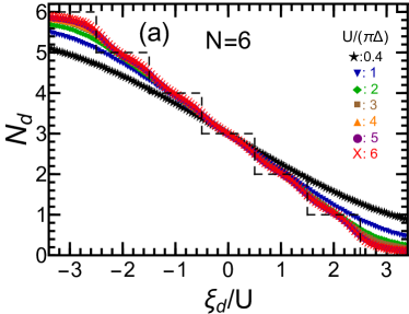
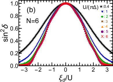
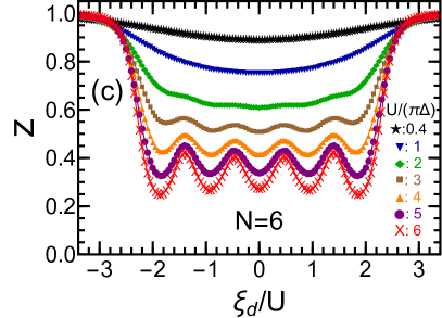
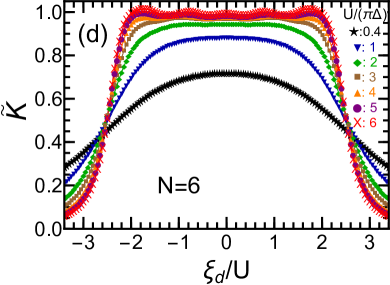
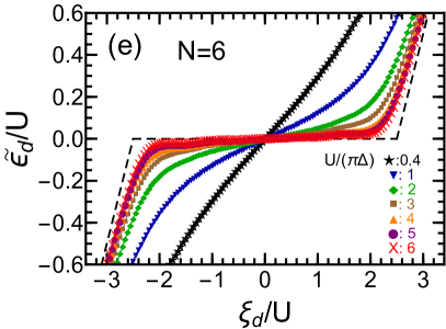
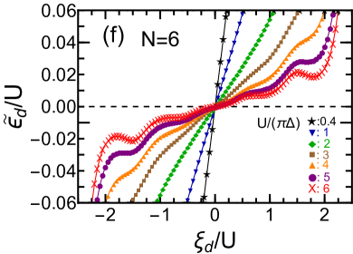
Figure 15: Fermi-liquid parameters for the SU(6) symmetric Anderson model are plotted vs $\xi_{d}$: (a) $N_{d}$, (b) $\sin^{2}\delta$, (c) renormalization factor $z$, (d) $\widetilde{K}=(N-1)(R-1)$. (e) renormalized level $\widetilde{\epsilon}_{d}$, and (f) enlarged view of $\widetilde{\epsilon}_{d}$, Interaction strengths are chosen to be $U/(\pi\Delta)=2/5(\star),1(\blacktriangledown),2(\blacklozenge),3(\blacksquare),4(\blacktriangle),5(\bullet),6(\times)$. The dashed line in (a) represents $N_{d}$ in the atomic limit $\Delta\to 0$.

Appendix D Two-body FL parameters for
SU(4) & SU(6) symmetric cases

We provide a quick overview of the behavior of the renormalized parameters in the SU(4) and SU(6) cases, which can be derived from the phase shift and the linear susceptibilities Nishikawa et al. (2010a, b); Oguri et al. (2011); Oguri (2012). Our discussion here is based on the the NRG results, plotted in Figs. 14 and 15 as functions of the impurity level position $\xi_{d}$, for several different interaction strengths: from weak to strong interactions up to $U/(\pi\Delta)=6.0$.

The SU($N$) Kondo effect occurs for strong interactions when the impurity levels are filled by an integer number of electrons, i.e., at the fillings of $N_{d}=1$, $2$, $\ldots$, $N-1$. It takes place at $\xi_{d}\simeq 0$, $\pm U$, …, $\pm\frac{N-2}{2}U$, and gives an interesting variety in the low-energy properties. As $N$ increases, a greater interaction strength is required to clearly observe the Kondo behavior. This is because the quantum fluctuations caused by the Coulomb interaction are suppressed for large $N$. In particular, the mean-field theory becomes exact in the limit $N\to\infty$ that is taken keeping the scaled interaction $U^{*}\equiv(N-1)U$ constant.Oguri (2012)

Figures 14(a) and 15(a) show the occupation number $N_{d}$ for $N=4$ and $6$, respectively. As $U$ increases, the Coulomb staircase structure emerges: $N_{d}$ varies steeply at $\xi_{d}\simeq\pm U/2$, $\pm 3U/2$, $\ldots$, $\pm(N-1)U/2$. Correspondingly, as $U$ increases, the transmission probability $\sin^{2}\delta$, shown in Figs. 14(b) and 15(b), exhibits a plateau structure that develops around $\xi_{d}\simeq 0$, $\pm U$, $\ldots$, $\pm(N-2)U/2$. In particular, the plateau at the half filling point $\xi_{d}\simeq 0$ reaches the unitary limit value $\sin^{2}\delta=1.0$.

The renormalization factor $z$, shown in Figs. 14(c) and 15(c) for $N=4$ and $6$, exhibits a broad valley structure at $|\xi_{d}|\lesssim(N-1)U/2$, where $1\lesssim N_{d}\lesssim N-1$. The valley becomes deeper as $U$ increases, and the local minima emerge for $U/(\pi\Delta)\gtrsim 3.0$ at the integer-filling points, reflecting the occurrence of the SU($N$) Kondo effects. The renormalization factor also has local maxima at intermediate valence states in between two adjacent local minima. Note that $z$ is significantly suppressed by the strong electron correlations even at these local maxima. Figures 14(d) and 15(d) show the rescaled Wilson ratio $\widetilde{K}\equiv(N-1)(R-1)$. For large interactions, $\widetilde{K}$ exhibits a wide flat structure at $|\xi_{d}|\lesssim(N-1)U/2$, the height of which approaches the saturation value $\widetilde{K}\simeq 1.0$, especially for $U/(\pi\Delta)\gtrsim 3.0$, reflecting the suppression of charge fluctuations in this region of $\xi_{d}$.

Figures 14(e) and 15(e) show the renormalized resonance-level position $\widetilde{\epsilon}_{d}\equiv z\Delta\cot\delta$ for $N=4$ and $6$, respectively, as a function of $\xi_{d}$. For strong interactions, the renormalized level is almost locked at the Fermi level, $\widetilde{\epsilon}_{d}\simeq 0.0$, in the strong-coupling region $|\xi_{d}|\lesssim(N-1)U/2$, which corresponds to the filling range of $1\lesssim N_{d}\lesssim N-1$. Figures 14(f) and 15(f) show an enlarged view of $\widetilde{\epsilon}_{d}$ in the vicinity of the Fermi level. We see that $\widetilde{\epsilon}_{d}$ exhibits a fine structure which reflects the staircase behavior of the phase shift $\delta$ and the oscillatory behavior of the renormalization factor $z$. Outside the strong-coupling region, $\widetilde{\epsilon}_{d}$ approaches the bare value $\widetilde{\epsilon}_{d}\simeq\epsilon_{d}$ at $\xi_{d}\gg(N-1)U/2$, or the Hatree-Fock value $\widetilde{\epsilon}_{d}\simeq\epsilon_{d}+(N-1)U$ at $\xi_{d}\ll-(N-1)U/2$: these asymptotic forms of $\widetilde{\epsilon}_{d}$ are shown as the dashed lines in Figs. 14(e) and 15(e).

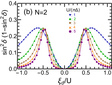
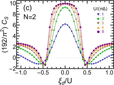
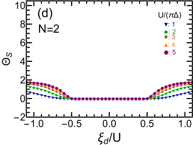
Figure 16: Current noise for SU(2) symmetric quantum dots vs $\xi_{d}$: (a) $\sin^{2}\delta$, (b) linear noise $\sin^{2}\delta\,(1-\sin^{2}\delta)$, (c) $(192/\pi^{2})\,C_{S}=W_{S}+\Theta_{S}$, (d) $\Theta_{S}=-\bigl{(}\Theta_{\mathrm{I}}+3\,\widetilde{\Theta}_{\mathrm{II}}\bigr{)}\cos 2\delta$ (see table 2). Interaction strengths are chosen to be $U/(\pi\Delta)=1(\blacktriangledown),2(\blacklozenge),3(\blacksquare),4(\blacktriangle),5(\bullet)$.

Appendix E Current noise and thermoelectric transport for SU(2) symmetric case

We have discussed the behavior of the current noise and thermo electric transport of the SU(4) and SU(6) Anderson model in Secs. VII, VIII, and X. For comparison, here we briefly describe the corresponding results in the SU(2) case, specifically, the current noise and the thermoelectric transport coefficients are plotted in Figs. 16 and 17, respectively.

We can see in Fig. 16(b) that the linear noise is suppressed in the strong-coupling region $|\xi_{d}|\lesssim U/2$ for large $U$, where the transmission probability exhibits a wide Kondo plateau in Fig. 16(a). However, the linear noise increases and has the peaks, the width of which is of the order of $\Delta$ at valence fluctuation regions near the quarter and three-quarters filling points where the phase reaches $\delta=\pi/4$ or $3\pi/4$. At these filling points, the coefficient $C_{S}$ for the order $|eV|^{3}$ nonlinear current noise has the negative minima, as seen in Fig. 16(c). We see in Fig. 16(d) that the three-body part $\Theta_{S}$ of $C_{S}$, is also suppressed over a wide region $|\xi_{d}|\lesssim U/2$. Therefore, in this strong-coupling region, the nonlinear noise $C_{S}$ is determined solely by the two-body part $W_{S}$ in the SU(2) case:

$$W_{S}\,=\,4(R-1)^{2}+\Bigl{[}\,1+5(R-1)^{2}\Bigr{]}\cos 4\delta\,,$$ (118)

where $R$ is the Wilson ratio. In particular, the dip structures of $C_{S}$ at the quarter and three-quarters fillings reflect the mimina of $\cos 4\delta$ in $W_{S}$. In contrast, at $|\xi_{d}|\gtrsim U/2$, the three-body part $\Theta_{S}$ becomes comparable to $W_{S}$, and contributes to $C_{S}$.

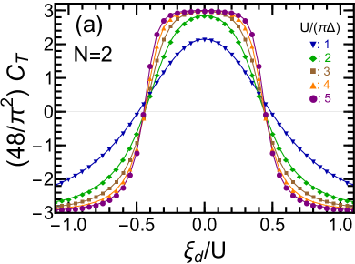
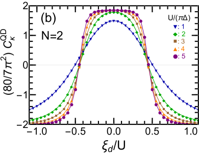
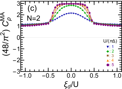
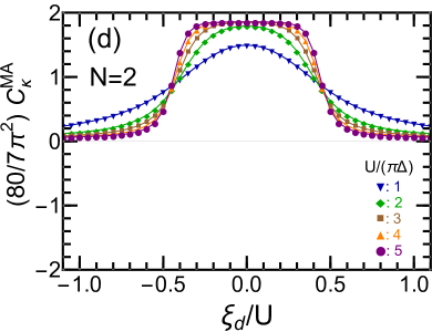
Figure 17: Next-leading order terms of transport coefficients for an SU(2) symmetric Anderson impurity: (a) $(48/\pi^{2})C_{T}$, (b) $[80/(7\pi^{2})]C_{\kappa}^{\mathrm{QD}}$, (c) $(48/\pi^{2})C_{\varrho}^{\mathrm{MA}}$, and (b) $[80/(7\pi^{2})]C_{\kappa}^{\mathrm{MA}}$, defined in table 2. Interaction strengths are chosen to be $U/(\pi\Delta)=1(\blacktriangledown),2(\blacklozenge),3(\blacksquare),4(\blacktriangle),5(\bullet)$.

Figure 17 shows the results for the next-leading order terms of the thermoelectric transport coefficients for the SU(2) quantum dots (a) $C_{T}$ and (b) $C_{\kappa}^{\mathrm{QD}}$, and for SU(2) magnetic alloys (c) $C_{\varrho}^{\mathrm{MA}}$ and (d) $C_{\kappa}^{\mathrm{MA}}$. All these coefficients exhibit the plateau structures due to the Kondo effect in the strong-coupling region $|\xi_{d}|\lesssim U/2$ for large $U$, where the phase shit is locked at $\delta\simeq\pi/2$. In this region, the three-body contributions, $\Theta_{\mathrm{I}}$ and $\widetilde{\Theta}_{\mathrm{II}}$, almost vanish (see Ref. Tsutsumi et al., 2021 for more details), and the height of these plateaus approach the saturation values for $U\to\infty$, i.e., $(48/\pi^{2})C_{T}\to 3$, $(48/\pi^{2})C_{\varrho}^{\mathrm{MA}}\to 3$, $[80/(7\pi^{2})]C_{\kappa}^{\mathrm{QD}}\to 13/7$, and $[80/(7\pi^{2})]C_{\kappa}^{\mathrm{MA}}\to 13/7$. The coefficients $C_{T}$ and $C_{\varrho}^{\mathrm{MA}}$ for charge transport show a similar behavior in the strong-coupling region. Furthermore, in this region, the coefficients for thermal conductivities, $C_{\kappa}^{\mathrm{QD}}$ and $C_{\kappa}^{\mathrm{MA}}$, also show a similar behavior. In contrast, at $|\xi_{d}|\gtrsim U/2$, the coefficients $C_{T}$ and $C_{\kappa}^{\mathrm{QD}}$ for quantum dots change sign and become negative as the occupation number approaches $N_{d}\simeq 0.0$ or $2.0$, whereas the coefficients $C_{\varrho}^{\mathrm{MA}}$ and $C_{\kappa}^{\mathrm{MA}}$ for magnetic alloys remain positive definite.

Appendix F Three-body Fermi-liquid corrections to thermoelectric transport of magnetic alloys

In this appendix, we describe the low-energy asymptotic form of electrical resistivity $\varrho_{\mathrm{MA}}=1/\sigma_{\mathrm{MA}}$, thermopower $\mathcal{S}_{\mathrm{MA}}$, and thermal conductivity $\kappa_{\mathrm{MA}}$ of magnetic alloys:

$$\sigma_{\mathrm{MA}}\ = \ \sigma_{\mathrm{MA}}^{\mathrm{unit}}\,\frac{1}{N}\,\sum_{\sigma}\mathcal{L}_{0,\sigma}^{\mathrm{MA}}\,,$$ (119)

$$\mathcal{S}_{\mathrm{MA}}\ = \ \frac{-1}{|e|T}\frac{\sum_{\sigma}\mathcal{L}_{1,\sigma}^{\mathrm{MA}}}{\sum_{\sigma}\mathcal{L}_{0,\sigma}^{\mathrm{MA}}}\,,$$ (120)

$$\kappa_{\mathrm{MA}}\ = \ \frac{\sigma_{\mathrm{MA}}^{\mathrm{unit}}}{e^{2}T}\,\frac{1}{N}\,\left[\,\sum_{\sigma}\mathcal{L}_{2,\sigma}^{\mathrm{MA}}-\frac{\left(\sum_{\sigma}\mathcal{L}_{1,\sigma}^{\mathrm{MA}}\right)^{2}}{\sum_{\sigma}\mathcal{L}_{0,\sigma}^{\mathrm{MA}}}\,\right].$$ (121)

For magnetic alloys, the response functions $\mathcal{L}_{n,\sigma}^{\mathrm{MA}}$ for $n=0,1$ and $2$ are given by

$$\mathcal{L}_{n,\sigma}^{\mathrm{MA}}=\int_{-\infty}^{\infty}d\omega\,\frac{\omega^{n}}{\pi\Delta A_{\sigma}(\omega)}\left(-\frac{\partial f(\omega)}{\partial\omega}\right).$$ (122)

Equation (119) defines the electrical conductivity relative to its unitary-limit value $\sigma_{\mathrm{MA}}^{\mathrm{unit}}$. Correspondingly, the prefactor for $\kappa_{\mathrm{MA}}$ is defined in such a way that the $T$-linear thermal conductivity should take the form,

$$\lim_{T\to 0}\frac{\kappa_{\mathrm{MA}}}{T}=\frac{\pi^{2}}{3\,e^{2}}\,\sigma_{\mathrm{MA}}^{\mathrm{unit}}\,.$$ (123)

The asymptotic form of $\mathcal{L}_{n,\sigma}^{\mathrm{MA}}$ can be calculated, using the low-energy expansion of the inverse spectral function $1/A_{\sigma}(\omega)$ given in Eq. (112):

$$\mathcal{L}_{0,\sigma}^{\mathrm{MA}}= \ \frac{1}{\sin^{2}\delta_{\sigma}}\left[\,1+\frac{a_{0,\sigma}^{\mathrm{MA}}}{\sin^{2}\delta_{\sigma}}\left(\pi T\right)^{2}\,\right]\ +\ \cdots\,,$$ (124)

$$\mathcal{L}_{1,\sigma}^{\mathrm{MA}}\,= \ -\frac{1}{3}\frac{\rho_{d\sigma}^{\prime}}{\pi\Delta\rho_{d\sigma}^{2}}\,(\pi T)^{2}\ +\ \cdots\,,$$ (125)

$$\mathcal{L}_{2,\sigma}^{\mathrm{MA}}= \ \frac{\left(\pi T\right)^{2}}{3\sin^{2}\delta_{\sigma}}\left[\,1+\frac{a_{2,\sigma}^{\mathrm{MA}}}{\sin^{2}\delta_{\sigma}}\left(\pi T\right)^{2}\,\right]\ +\ \cdots\,.$$ (126)

Here, the coefficients $a_{0,\sigma}^{\mathrm{MA}}$ and $a_{2,\sigma}^{\mathrm{MA}}$ are given by

$$\!\!\!a_{0,\sigma}^{\mathrm{MA}}= \,\frac{\pi^{2}}{3}\Biggl{[}\left(\cos 2\delta_{\sigma}+2\right)\chi_{\sigma\sigma}^{2}-2\cos 2\delta_{\sigma}\,\sum_{\sigma^{\prime}(\neq\sigma)}\chi_{\sigma\sigma^{\prime}}^{2}$$

$$\ \ +\frac{\sin 2\delta_{\sigma}}{2\pi}\,\left(\chi_{\sigma\sigma\sigma}^{[3]}+\sum_{\sigma^{\prime}(\neq\sigma)}\chi_{\sigma\sigma^{\prime}\sigma^{\prime}}^{[3]}\right)\Biggr{]},$$ (127)

$$\!\!\!a_{2,\sigma}^{\mathrm{MA}}= \,\frac{7\pi^{2}}{5}\Biggl{[}\left(\cos 2\delta_{\sigma}+2\right)\chi_{\sigma\sigma}^{2}-\frac{6}{7}\cos 2\delta_{\sigma}\sum_{\sigma^{\prime}(\neq\sigma)}\chi_{\sigma\sigma^{\prime}}^{2}$$

$$\ \ +\frac{\sin 2\delta_{\sigma}}{2\pi}\left(\chi_{\sigma\sigma\sigma}^{[3]}+\frac{5}{21}\sum_{\sigma^{\prime}(\neq\sigma)}\chi_{\sigma\sigma^{\prime}\sigma^{\prime}}^{[3]}\right)\Biggr{]}.$$ (128)

We obtain the low-temperature expressions of $\varrho_{\mathrm{MA}}=1/\sigma_{\mathrm{MA}}$, $\mathcal{S}_{\mathrm{MA}}$ and $1/\kappa_{\mathrm{MA}}$, substituting Eqs. (124)–(126) into Eqs. (119)–(121):

$$\varrho_{\mathrm{MA}}= \,\frac{1}{\sigma_{\mathrm{MA}}^{\mathrm{unit}}}\,\left[\,\bigl{(}\overline{\sin^{2}\delta}\bigr{)}_{\mathrm{HM}}-c_{\varrho}^{\mathrm{MA}}\,\left(\pi T\right)^{2}+\cdots\right],$$ (129)

$$\mathcal{S}_{\mathrm{MA}}= \,\frac{\pi^{2}}{3}\,\frac{\sum_{\sigma}\rho_{d\sigma}^{\prime}}{\sum_{\sigma}\rho_{d\sigma}}\,\frac{T}{|e|}\,+\,\cdots,$$ (130)

$$\frac{1}{\kappa_{\mathrm{MA}}}\,= \,\frac{3\,e^{2}}{\pi^{2}\,\sigma_{\mathrm{MA}}^{\mathrm{unit}}}\,\frac{1}{T}\,\Bigl{[}\,\bigl{(}\overline{\sin^{2}\delta}\bigr{)}_{\mathrm{HM}}\,-\,c_{\kappa}^{\mathrm{MA}}\,\left(\pi T\right)^{2}\,+\,\cdots\,\Bigr{]}.$$ (131)

Here, $\bigl{(}\overline{\sin^{2}\delta}\bigr{)}_{\mathrm{HM}}$ is the harmonic mean (HM) of $\sin^{2}\delta_{\sigma}$, defined by

$$\bigl{(}\overline{\sin^{2}\delta}\bigr{)}_{\mathrm{HM}}\,\equiv\,\frac{1}{\frac{1}{N}\,\sum_{\sigma}\,\frac{1}{\sin^{2}\delta_{\sigma}}}\,.$$ (132)

The coefficients $c_{\varrho}^{\mathrm{MA}}$ and $c_{\kappa}^{\mathrm{MA}}$ of the next leading-order terms are given by

$$c_{\varrho}^{\mathrm{MA}}\,= \,\left\{\bigl{(}\overline{\sin^{2}\delta}\bigr{)}_{\mathrm{HM}}\right\}^{2}\frac{1}{N}\,\sum_{\sigma}\,\frac{a_{0,\sigma}^{\mathrm{MA}}}{\sin^{4}\delta_{\sigma}}\,,$$ (133)

$$c_{\kappa}^{\mathrm{MA}}\,= \,\left\{\bigl{(}\overline{\sin^{2}\delta}\bigr{)}_{\mathrm{HM}}\right\}^{2}\left[\frac{1}{N}\,\sum_{\sigma}\,\frac{a_{2,\sigma}^{\mathrm{MA}}}{\sin^{4}\delta_{\sigma}}\,\right.$$

$$\left.\,-\,\frac{\pi^{2}}{3}\,\bigl{(}\overline{\sin^{2}\delta}\bigr{)}_{\mathrm{HM}}\left\{\frac{1}{N}\,\sum_{\sigma}\,\frac{\sin 2\delta_{\sigma}}{\sin^{4}\delta_{\sigma}}\,\chi_{\sigma\sigma}\right\}^{2}\,\right].$$ (134)

Correspondingly, the electrical conductivity and the thermal conductivity take the following form,

$$\sigma_{\mathrm{MA}}\,= \,\frac{\sigma_{\mathrm{MA}}^{\mathrm{unit}}}{\bigl{(}\overline{\sin^{2}\delta}\bigr{)}_{\mathrm{HM}}}\,\left[\,1\,+\frac{c_{\varrho}^{\mathrm{MA}}}{\bigl{(}\overline{\sin^{2}\delta}\bigr{)}_{\mathrm{HM}}}\,\left(\pi T\right)^{2}\,+\,\cdots\,\right],$$ (135)

$$\mathcal{\kappa}_{\mathrm{MA}}= \,\frac{\pi^{2}\,\sigma_{\mathrm{MA}}^{\mathrm{unit}}}{3\,e^{2}}\,\frac{T}{\bigl{(}\overline{\sin^{2}\delta}\bigr{)}_{\mathrm{HM}}}$$

$$\qquad\times\left[\,1\,+\,\frac{c_{\kappa}^{\mathrm{MA}}}{\bigl{(}\overline{\sin^{2}\delta}\bigr{)}_{\mathrm{HM}}}\,\left(\pi T\right)^{2}\,+\,\cdots\,\right].$$ (136)

Furthermore, the Lorenz number $L_{\mathrm{MA}}\equiv\kappa_{\mathrm{MA}}/(\sigma_{\mathrm{MA}}T)$ can also be deduced up to terms of order $T^{2}$, as

$$L_{\mathrm{MA}}\,\,= \ \frac{\pi^{2}}{3\,e^{2}}\,\left[1\,-\,\frac{c_{L}^{\mathrm{MA}}}{\bigl{(}\overline{\sin^{2}\delta}\bigr{)}_{\mathrm{HM}}}\,\left(\pi T\right)^{2}\ +\ \cdots\,\right],$$ (137)

$$c_{L}^{\mathrm{MA}}\,= \ c_{\varrho}^{\mathrm{MA}}\,-\,c_{\kappa}^{\mathrm{MA}}\,.$$ (138)

In the limit of zero temperature, the Lorenz number takes a constant value $L_{\mathrm{MA}}\xrightarrow{\,T\to 0\,}\frac{\pi^{2}}{3\,e^{2}}$, and the Wiedemann-Franz law holds. However, it deviates as temperature increases, showing the $T^{2}$ dependence.

Appendix G Thermoelectric transport coefficients for noninteracting magnetic alloys

We provide here the noninteracting results for the thermoelectric transport coefficients of magnetic alloys. For $U=0$, the response functions $\mathcal{L}_{n,\sigma}^{\mathrm{MA}}$ for $n=0,1,2$ can be calculated, substituting the explicit form of the spectral function $\pi A_{\sigma}(\omega)\xrightarrow{\,U=0\,}\Delta/[(\omega-\epsilon_{d\sigma})^{2}+\Delta^{2}]$ into Eq. (122):

$$\mathcal{L}_{0,\sigma}^{\mathrm{MA}}\,\xrightarrow{\,U=0\,} \ \left[1+\left(\frac{\epsilon_{d\sigma}}{\Delta}\right)^{2}\right]\,+\,\frac{1}{3}\left(\frac{\pi T}{\Delta}\right)^{2},$$ (139)

$$\mathcal{L}_{1,\sigma}^{\mathrm{MA}}\,\xrightarrow{\,U=0\,} \ \frac{-2\,\epsilon_{d\sigma}}{3}\left(\frac{\pi T}{\Delta}\right)^{2},$$ (140)

$$\mathcal{L}_{2,\sigma}^{\mathrm{MA}}\,\xrightarrow{\,U=0\,} \ \frac{\Delta^{2}}{3}\left[1+\left(\frac{\epsilon_{d\sigma}}{\Delta}\right)^{2}\right]\left(\frac{\pi T}{\Delta}\right)^{2}+\frac{7\Delta^{2}}{15}\left(\frac{\pi T}{\Delta}\right)^{4}.$$ (141)

The transport coefficients, defined in Eqs. (119)–(121), can be deduced from these analytic expressions for $\mathcal{L}_{n,\sigma}^{\mathrm{MA}}$. In particular, in the SU($N$) symmetric case where $\epsilon_{d\sigma}\equiv\epsilon_{d}$, the electrical resistivity $\varrho_{\mathrm{MA}}^{(0)}$ for $U=0$ is given by ,

$$\varrho_{\mathrm{MA}}^{(0)}\,=\,\frac{1}{\sigma_{\mathrm{MA}}^{\mathrm{unit}}}\,\left[\,\sin^{2}\delta_{0}\,-\,C_{\varrho}^{\mathrm{MA}(0)}\,\left(\frac{\pi T}{T^{*}_{0}}\right)^{2}\,\right],$$ (142)

$$\sin^{2}\delta_{0}\,=\,\frac{1}{1+(\epsilon_{d}/\Delta)^{2}}\qquad C_{\varrho}^{\mathrm{MA}(0)}\,=\,\frac{\pi^{2}}{48}\,.$$ (143)

Here, $T_{0}^{*}\equiv\pi\Delta/(4\sin^{2}\delta_{0})$ is the characteristic energy scale in the noninteracting case. The coefficient $C_{\varrho}^{\mathrm{MA}(0)}$ for the $T^{2}$-resistivity is given by a constant $\pi^{2}/48$ ($=0.205\cdots$) as the $\epsilon_{d}$-dependence is absorbed into $T_{0}^{*}$.

The thermopower $\mathcal{S}_{\mathrm{QD}}^{0}$ and thermal resistivity $1/\kappa_{\mathrm{MA}}^{(0)}$ for $U=0$ are given by

$$\mathcal{S}_{\mathrm{MA}}^{(0)}\,=\,\frac{1}{|e|}\,\frac{2\pi^{2}}{3}\,\frac{\epsilon_{d}}{\epsilon_{d}^{2}+\Delta^{2}}\,T\;,$$ (144)

$$\frac{1}{\kappa_{\mathrm{MA}}^{(0)}}\,=\,\frac{3\,e^{2}}{\pi^{2}\,\sigma_{\mathrm{MA}}^{\mathrm{unit}}}\,\frac{1}{T}\,\left[\,\sin^{2}\delta_{0}\,-\,C_{\kappa}^{\mathrm{MA}(0)}\,\left(\frac{\pi T}{T_{0}^{*}}\right)^{2}\,\right],$$ (145)

$$C_{\kappa}^{\mathrm{MA}(0)}\,=\,\frac{7\pi^{2}}{80}\,\frac{1+20\sin^{2}\delta_{0}}{21}\,.$$ (146)

Furthermore, the dimensionless coefficient for the order $T^{2}$ term of the Lorenz number $L_{\mathrm{MA}}$ is given by $C_{L}^{\mathrm{MA}(0)}\equiv C_{\varrho}^{\mathrm{MA}(0)}-C_{\kappa}^{\mathrm{MA}(0)}$ and it takes the form,

$$C_{L}^{\mathrm{MA}(0)}\,=\,\frac{\pi^{2}}{60}\,\left(\,1-5\sin^{2}\delta_{0}\,\right)\,.$$ (147)

These results for the next-leading order terms in the noninterating case are plotted as functions of $\epsilon_{d}$ in Fig.  18. The coefficient $C_{\kappa}^{\mathrm{MA}(0)}$ takes a Lorentzian form with an offset value of $C_{\kappa}^{\mathrm{MA}(0)}\xrightarrow{\,|\epsilon_{d}|\to\infty\,}\pi^{2}/240$ ($=0.041\cdots$). Correspondingly, $C_{L}^{\mathrm{MA}(0)}$ has a dip at $\epsilon_{d}=0$, and vanishes at the points $\epsilon_{d}=\pm 2\Delta$ where $C_{\kappa}^{\mathrm{MA}(0)}$ and $C_{\varrho}^{\mathrm{MA(0)}}$ give equal contributions to the Lonrez number $L_{\mathrm{MA}}$. As the impurity level moves further away from the Fermi level $|\epsilon_{d}|\gg\Delta$, it approaches the value of $C_{L}^{\mathrm{MA}(0)}\xrightarrow{\,|\epsilon_{d}|\to\infty\,}\pi^{2}/60$ ($=0.164\cdots$).

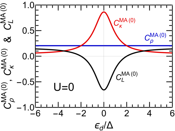
Figure 18: Coefficients $C_{\varrho}^{\mathrm{MA}(0)}$, $C_{\kappa}^{\mathrm{MA}(0)}$, and $C_{L}^{\mathrm{MA}(0)}$ for noninteracting $U=0$ magnetic alloys plotted vs $\epsilon_{d}$.

References

- Kondo (1964) J. Kondo, Prog. Theor. Phys. 32, 37 (1964).
- Hewson (1993) A. C. Hewson, The Kondo Problem to Heavy Fermions (Cambridge University Press, 1993).
- Ono et al. (2019) K. Ono, J. Kobayashi, Y. Amano, K. Sato, and Y. Takahashi, Phys. Rev. A 99, 032707 (2019).
- Yasui and Ozaki (2017) S. Yasui and S. Ozaki, Phys. Rev. D 96, 114027 (2017).
- Nozières (1974) P. Nozières, J. Low Temp. Phys. 17, 31 (1974).
- Yamada (1975a) K. Yamada, Prog. Theor. Phys. 53, 970 (1975a).
- Yamada (1975b) K. Yamada, Prog. Theor. Phys. 54, 316 (1975b).
- Shiba (1975) H. Shiba, Prog. Theor. Phys. 54, 967 (1975).
- Yoshimori (1976) A. Yoshimori, Prog. Theor. Phys. 55, 67 (1976).
- Wilson (1975) K. G. Wilson, Rev. Mod. Phys. 47, 773 (1975).
- Krishna-murthy et al. (1980a) H. R. Krishna-murthy, J. W. Wilkins, and K. G. Wilson, Phys. Rev. B 21, 1003 (1980a).
- Krishna-murthy et al. (1980b) H. R. Krishna-murthy, J. W. Wilkins, and K. G. Wilson, Phys. Rev. B 21, 1044 (1980b).
- Hershfield et al. (1992) S. Hershfield, J. H. Davies, and J. W. Wilkins, Phys. Rev. B 46, 7046 (1992).
- Oguri (2001) A. Oguri, Phys. Rev. B 64, 153305 (2001).
- Mora (2009) C. Mora, Phys. Rev. B 80, 125304 (2009).
- Mora et al. (2009) C. Mora, P. Vitushinsky, X. Leyronas, A. A. Clerk, and K. Le Hur, Phys. Rev. B 80, 155322 (2009).
- Mora et al. (2015) C. Mora, C. P. Moca, J. von Delft, and G. Zaránd, Phys. Rev. B 92, 075120 (2015).
- Filippone et al. (2017) M. Filippone, C. P. Moca, J. von Delft, and C. Mora, Phys. Rev. B 95, 165404 (2017).
- Oguri and Hewson (2018a) A. Oguri and A. C. Hewson, Phys. Rev. Lett. 120, 126802 (2018a).
- Oguri and Hewson (2018b) A. Oguri and A. C. Hewson, Phys. Rev. B 97, 045406 (2018b).
- Oguri and Hewson (2018c) A. Oguri and A. C. Hewson, Phys. Rev. B 97, 035435 (2018c).
- Karki and Kiselev (2017) D. B. Karki and M. N. Kiselev, Phys. Rev. B 96, 121403(R) (2017).
- Karki et al. (2018) D. B. Karki, C. Mora, J. von Delft, and M. N. Kiselev, Phys. Rev. B 97, 195403 (2018).
- Karki and Kiselev (2018) D. B. Karki and M. N. Kiselev, Phys. Rev. B 98, 165443 (2018).
- Moca et al. (2018) C. P. Moca, C. Mora, I. Weymann, and G. Zaránd, Phys. Rev. Lett. 120, 016803 (2018).
- Teratani et al. (2020a) Y. Teratani, R. Sakano, and A. Oguri, Phys. Rev. Lett. 125, 216801 (2020a).
- Oguri et al. (2022) A. Oguri, Y. Teratani, K. Tsutsumi, and R. Sakano, Phys. Rev. B 105, 115409 (2022).
- Tsutsumi et al. (2021) K. Tsutsumi, Y. Teratani, R. Sakano, and A. Oguri, Phys. Rev. B 104, 235147 (2021).
- Tsutsumi et al. (2023) K. Tsutsumi, Y. Teratani, K. Motoyama, R. Sakano, and A. Oguri, Phys. Rev. B 108, 045109 (2023).
- Glazman and Raikh (1988) L. I. Glazman and M. E. Raikh, JETP Lett. 47, 452 (1988).
- Ng and Lee (1988) T. K. Ng and P. A. Lee, Phys. Rev. Lett. 61, 1768 (1988).
- Wingreen and Meir (1994) N. S. Wingreen and Y. Meir, Phys. Rev. B 49, 11040 (1994).
- Meir and Wingreen (1992) Y. Meir and N. S. Wingreen, Phys. Rev. Lett. 68, 2512 (1992).
- Izumida et al. (1998) W. Izumida, O. Sakai, and Y. Shimizu, Journal of the Physical Society of Japan 67, 2444 (1998).
- Izumida et al. (2001) W. Izumida, O. Sakai, and S. Suzuki, J. Phys. Soc. Jpn. 70, 1045 (2001).
- Aligia (2012) A. A. Aligia, Journal of Physics: Condensed Matter 24, 015306 (2012).
- Aligia (2014) A. A. Aligia, Phys. Rev. B 89, 125405 (2014).
- Filippone et al. (2018) M. Filippone, C. P. Moca, A. Weichselbaum, J. von Delft, and C. Mora, Phys. Rev. B 98, 075404 (2018).
- Gogolin and Komnik (2006) A. O. Gogolin and A. Komnik, Phys. Rev. Lett. 97, 016602 (2006).
- Sela et al. (2006) E. Sela, Y. Oreg, F. von Oppen, and J. Koch, Phys. Rev. Lett. 97, 086601 (2006).
- Golub (2006) A. Golub, Phys. Rev. B 73, 233310 (2006).
- Sela and Malecki (2009) E. Sela and J. Malecki, Phys. Rev. B 80, 233103 (2009).
- Sakano et al. (2011) R. Sakano, T. Fujii, and A. Oguri, Phys. Rev. B 83, 075440 (2011).
- Costi et al. (1994) T. A. Costi, A. C. Hewson, and V. Zlatić, J. Phys.: Condens. Matter 6, 2519 (1994).
- Costi (2019) T. A. Costi, Phys. Rev. B 100, 155126 (2019).
- Goldhaber-Gordon et al. (1998a) D. Goldhaber-Gordon, H. Shtrikman, D. Mahalu, D. Abusch-Magder, U. Meirav, and M. A. Kastner, Nature 391, 156 (1998a).
- Goldhaber-Gordon et al. (1998b) D. Goldhaber-Gordon, J. Göres, M. A. Kastner, H. Shtrikman, D. Mahalu, and U. Meirav, Phys. Rev. Lett. 81, 5225 (1998b).
- Cronenwett et al. (1998) S. M. Cronenwett, T. H. Oosterkamp, and L. P. Kouwenhoven, Science 281, 540 (1998).
- van der Wiel et al. (2000) W. G. van der Wiel, S. D. Franceschi, T. Fujisawa, J. M. Elzerman, S. Tarucha, and L. P. Kouwenhoven, Science 289, 2105 (2000).
- V. Borzenets et al. (2020) I. V. Borzenets, J. Shim, J. C. H. Chen, A. Ludwig, A. D. Wieck, S. Tarucha, H.-S. Sim, and M. Yamamoto, Nature 579, 210 (2020).
- Grobis et al. (2008) M. Grobis, I. G. Rau, R. M. Potok, H. Shtrikman, and D. Goldhaber-Gordon, Phys. Rev. Lett. 100, 246601 (2008).
- Scott et al. (2009) G. D. Scott, Z. K. Keane, J. W. Ciszek, J. M. Tour, and D. Natelson, Phys. Rev. B 79, 165413 (2009).
- Zarchin et al. (2008) O. Zarchin, M. Zaffalon, M. Heiblum, D. Mahalu, and V. Umansky, Phys. Rev. B 77, 241303(R) (2008).
- Delattre et al. (2009) T. Delattre, C. Feuillet-Palma, L. G. Herrmann, P. Morfin, J.-M. Berroir, G. FShu ve, B. PlaXun ais, D. C. Glattli, M.-S. Choi, C. Mora, and T. Kontos, Nature Physics 5, 208 (2009).
- Yamauchi et al. (2011) Y. Yamauchi, K. Sekiguchi, K. Chida, T. Arakawa, S. Nakamura, K. Kobayashi, T. Ono, T. Fujii, and R. Sakano, Phys. Rev. Lett. 106, 176601 (2011).
- Ferrier et al. (2016) M. Ferrier, T. Arakawa, T. Hata, R. Fujiwara, R. Delagrange, R. Weil, R. Deblock, R. Sakano, A. Oguri, and K. Kobayashi, Nat. Phys. 12, 230 (2016).
- Hata et al. (2021) T. Hata, Y. Teratani, T. Arakawa, S. Lee, M. Ferrier, R. Deblock, R. Sakano, A. Oguri, and K. Kobayashi, Nature Communications 12, 3233 (2021).
- Hsu et al. (2022) C. Hsu, T. A. Costi, D. Vogel, C. Wegeberg, M. Mayor, H. S. J. van der Zant, and P. Gehring, Phys. Rev. Lett. 128, 147701 (2022).
- Svilans et al. (2018) A. Svilans, M. Josefsson, A. M. Burke, S. Fahlvik, C. Thelander, H. Linke, and M. Leijnse, Phys. Rev. Lett. 121, 206801 (2018).
- Laird et al. (2015) E. A. Laird, F. Kuemmeth, G. A. Steele, K. Grove-Rasmussen, J. Nygård, K. Flensberg, and L. P. Kouwenhoven, Rev. Mod. Phys. 87, 703 (2015).
- Borda et al. (2003) L. Borda, G. Zaránd, W. Hofstetter, B. I. Halperin, and J. von Delft, Phys. Rev. Lett. 90, 026602 (2003).
- Choi et al. (2005) M.-S. Choi, R. López, and R. Aguado, Phys. Rev. Lett. 95, 067204 (2005).
- Eto (2005) M. Eto, Journal of the Physical Society of Japan 74, 95 (2005).
- Sakano and Kawakami (2006) R. Sakano and N. Kawakami, Phys. Rev. B 73, 155332 (2006).
- Anders et al. (2008) F. B. Anders, D. E. Logan, M. R. Galpin, and G. Finkelstein, Phys. Rev. Lett. 100, 086809 (2008).
- Weymann et al. (2018) I. Weymann, R. Chirla, P. Trocha, and C. P. Moca, Phys. Rev. B 97, 085404 (2018).
- Filippone et al. (2014) M. Filippone, C. P. Moca, G. Zaránd, and C. Mora, Phys. Rev. B 90, 121406(R) (2014).
- Mantelli et al. (2016) D. Mantelli, C. P. Moca, G. Zarand, and M. Grifoni, Physica E: Low-dimensional Systems and Nanostructures 77, 180 (2016).
- Teratani et al. (2020b) Y. Teratani, R. Sakano, T. Hata, T. Arakawa, M. Ferrier, K. Kobayashi, and A. Oguri, Phys. Rev. B 102, 165106 (2020b).
- Sasaki et al. (2000) S. Sasaki, S. De Franceschi, J. M. Elzerman, W. G. van der Wiel, M. Eto, S. Tarucha, and L. P. Kouwenhoven, Nature 405, 764 (2000).
- Jarillo-Herrero et al. (2005) P. Jarillo-Herrero, J. Kong, H. S. J. van der Zant, C. Dekker, L. P. Kouwenhoven, and S. De Franceschi, Phys. Rev. Lett. 94, 156802 (2005).
- Babić et al. (2004) B. Babić, T. Kontos, and C. Schönenberger, Phys. Rev. B 70, 235419 (2004).
- Makarovski et al. (2007) A. Makarovski, A. Zhukov, J. Liu, and G. Finkelstein, Phys. Rev. B 75, 241407(R) (2007).
- Cleuziou et al. (2013) J. P. Cleuziou, N. V. N’Guyen, S. Florens, and W. Wernsdorfer, Phys. Rev. Lett. 111, 136803 (2013).
- Kuzmenko et al. (2006) T. Kuzmenko, K. Kikoin, and Y. Avishai, Phys. Rev. B 73, 235310 (2006).
- López et al. (2013) R. López, T. Rejec, J. Martinek, and R. Žitko, Phys. Rev. B 87, 035135 (2013).
- Kuzmenko and Avishai (2014) I. Kuzmenko and Y. Avishai, Phys. Rev. B 89, 195110 (2014).
- Caroli et al. (1971) C. Caroli, R. Combescot, and P. Nozières, Phys. C: Solid State Phys 4, 916 (1971).
- Hershfield (1992) S. Hershfield, Phys. Rev. B 46, 7061 (1992).
- Guttman et al. (1995) G. D. Guttman, E. Ben-Jacob, and D. J. Bergman, Phys. Rev. B 51, 17758 (1995).
- Costi and Zlatić (2010) T. A. Costi and V. Zlatić, Phys. Rev. B 81, 235127 (2010).
- Chirla and Moca (2014) R. Chirla and C. P. Moca, Phys. Rev. B 89, 045132 (2014).
- Pérez Daroca et al. (2018) D. Pérez Daroca, P. Roura-Bas, and A. A. Aligia, Phys. Rev. B 97, 165433 (2018).
- Hewson (2001) A. C. Hewson, J. Phys.: Condens. Matter 13, 10011 (2001).
- Hewson et al. (2004) A. C. Hewson, A. Oguri, and D. Meyer, Eur. Phys. J. B 40, 177 (2004).
- Stadler et al. (2016) K. M. Stadler, A. K. Mitchell, J. von Delft, and A. Weichselbaum, Phys. Rev. B 93, 235101 (2016).
- Oliveira and Oliveira (1994) W. C. Oliveira and L. N. Oliveira, Phys. Rev. B 49, 11986 (1994).
- Nishikawa et al. (2010a) Y. Nishikawa, D. J. G. Crow, and A. C. Hewson, Phys. Rev. B 82, 115123 (2010a).
- Nishikawa et al. (2010b) Y. Nishikawa, D. J. G. Crow, and A. C. Hewson, Phys. Rev. B 82, 245109 (2010b).
- Oguri et al. (2011) A. Oguri, R. Sakano, and T. Fujii, Phys. Rev. B 84, 113301 (2011).
- Oguri (2012) A. Oguri, Phys. Rev. B 85, 155404 (2012).