Machine-learning-inspired quantum control in many-body dynamics
Abstract
Achieving precise preparation of quantum many-body states is crucial for the practical implementation of quantum computation and quantum simulation. However, the inherent challenges posed by unavoidable excitations at critical points during quench processes necessitate careful design of control fields. In this work, we introduce a promising and versatile dynamic control neural network tailored to optimize control fields. We address the problem of suppressing defect density and enhancing cat-state fidelity during the passage across the critical point in the quantum Ising model. Our method facilitates seamless transitions between different objective functions by adjusting the optimization strategy. In comparison to gradient-based power-law quench methods, our approach demonstrates significant advantages for both small system sizes and long-term evolutions. We provide a detailed analysis of the specific forms of control fields and summarize common features for experimental implementation. Furthermore, numerical simulations demonstrate the robustness of our proposal against random noise and spin number fluctuations. The optimized defect density and cat-state fidelity exhibit a transition at a critical ratio of the quench duration to the system size, coinciding with the quantum speed limit for quantum evolution.
I Introduction
Nowadays it is imperative to achieve precise preparation of quantum many-body states due to the urgent demand for applications in various fields, including quantum computation [1, 2] and quantum simulation [3, 4, 5]. In particular, quantum metrology, a rapidly advancing field of quantum information science, is currently experiencing a surge of theoretical developments [6, 7, 8] and experimental breakthroughs [9, 10, 11, 12]. A pivotal focus of a quantum metrology scheme involves the preparation of optimal nonclassical states [13, 14]. Through the utilization of inherent quantum properties, such as entanglement [15, 16, 17], coherence [18] and discord [19, 20], quantum metrology can achieve the sensitivity for estimating unknown parameters that surpasses the constraints imposed by the standard quantum limit of classical strategies 111If there are qubits in separable states, it is known that the uncertainty (that is, the inverse of the sensitivity) scales as , which is called the standard quantum limit, while quantum physics allows the ultimate scalings being , i.e., the Heisenberg scaling, in the absence of noise and in the presence of realistic decoherence. In fact, the enhanced sensitivity may even approach the limits set by the Heisenberg uncertainty principle [22]. To this end, various forms of entangled states have been generated in engineered many-body systems to increase the phase sensitivity [23, 24]. However, a comprehensive understanding of the relationship between quantum features and ultimate scaling sensitivity beyond the standard quantum limit remains elusive.
A widely employed method for the theoretical [25, 26, 27, 28, 29] and experimental [30, 31, 32, 33, 34] preparation of quantum many-body states involves utilizing unitary evolution. This process transforms the initial state, typically the ground state of some simple Hamiltonian , into the ground state of the target Hamiltonian . According to the adiabatic theorem, the unitary transformation can be implemented with arbitrary accuracy by changing the Hamiltonian sufficiently slowly [35, 36]. Nevertheless, the strict requirement of the adiabatic limit dictates infinitely long evolution time, inevitably resulting in system decoherence and the disappearance of entanglement [37]. In particular, crossing a quantum critical point (QCP) in finite time challenges the adiabatic condition due to the closing of the energy gap, which ultimately results in the formation of excitations [38]. Consequently, a trade-off must be considered between the evolution time and the excitations generated by the system. In this context, tremendous efforts have recently been dedicated to achieving an optimal passage through the non-adiabatic evolution, particularly across the QCP, aiming to minimize unwanted excitations [39, 40] or to maximize fidelity [41, 42]. Shortcut to adiabaticity (STA) provides a way of finding fast trajectories that connect the initial and final states by manipulating the system’s parameters in a non-adiabatic fashion while still obtaining results akin to those of an adiabatic process [43, 44, 45, 46, 47]. Given the flexibility in selecting intermediate trajectories, the time-dependent control parameters of a system can be adjusted in various STA protocols [48]. One common method of STA involves introducing counterdiabatic driving to the reference Hamiltonian that effectively compensates for the non-adiabatic behavior. However, implementing this technique in quantum many-body systems remains a challenging task for experimental execution.
Alternatively, a prevalent approach is quantum optimal control [49, 50, 51, 52, 53], where time-dependent control parameters of a system are fine-tuned using optimal control theory. Governed by time-energy uncertainty relations, the characteristic time scales during non-adiabatic evolution are encapsulated by the quantum speed limit [54, 55, 56], which delves into the minimum time required for quantum states to achieve specific predetermined objectives. This is particularly crucial in the field of quantum information, where rapid dynamics are often advantageous [57, 58, 56]. While the quantum optimal control finds widespread applications in various systems, it is of fundamental interest to formulate the control theory in a general framework. Over the past few years, machine-learning technology has become an integral part of the optimization theory and has been proved to be applicable to optimizing the parameters of variational states in a variety of interacting quantum many-body systems [59, 60, 61, 62, 63, 64]. In this work, we propose a promising and generalizable dynamic control neural network (DCNN) to optimize the control field passing through two fixed points of the quantum critical systems that holds potential for testing and comparing approximate methods, as well as bearing implications for condensed matter physics. To demonstrate the power of our method, we focus on suppressing the defect density and improving the cat-state fidelity during the passage across the critical point in the quantum Ising model. Compared to the gradient-based power-law quench [65], the method offers significant advantages over small system size and long-term evolution. We also numerically demonstrate that our proposal is robust against the random noise and the spin number fluctuations. The optimized defect density and cat-state fidelity are uncovered to coincide with the quantum speed limit for quantum evolution.
The rest of the paper is organized as follows. In Sec. II we present the gradients of specific observables with respect to the time-dependent control parameter in the many-body systems that can be transformed into free fermions. Additionally, we introduce the DCNN method in this section. Section III is devoted to the application of the DCNN to the suppression of the defect density in the quantum Ising model. A thorough analysis of achieving the optimized control fields is also discussed. The effectiveness of the protocol, particularly under varying conditions such as random noise and fluctuations in the number of spins, is evaluated through comprehensive numerical simulations. Section IV delves into the improvement of the cat-state fidelity in the quantum Ising model. Finally, the conclusion and outlook are given in Sec. V.
II Dynamical protocol in integrable many-body models
II.1 Quantum Ising-like models
The quantum Ising model has emerged as a prototypical model of quantum many-body systems due to its analytical solvability. It thus serves as a valuable tool for exploring emerging quantum phenomena [66, 67, 68, 69, 70, 71, 72] and as a benchmark for evaluating the effectiveness of state-of-the-art approaches and algorithms [73, 74, 75]. Furthermore, it is an especially compelling option as a versatile platform for quantum simulation [76, 77, 78, 79]. The exact simulation of Ising model has been implemented on quantum computers [80, 81]. Actually, the steps to build quantum circuits at a scale that could provide an advantage for simulating the Ising Hamiltonian follow the same strategy as the analytical solution of the models. Therefore, the method can be extended to other integrable models. To this end, we focus on a class of integrable many-body spin systems that can be mapped into free fermion models. A variety of systems holding quantum phase transitions can be mapped into such kinds of models, including the one-dimensional (1D) quantum Ising model and XY model, which is regarded as one of two canonical quantum critical systems [82], as well as the 1D and two-dimensional Kitaev models [83, 84], etc. These cover a variety of spin models that are of interest in both quantum information science and condensed matter physics.
Consider a closed quantum system which depends on time explicitly through a control field that can be varied arbitrarily with certain constraints. The control field is assumed to enter via a term with some time-independent operator. We consider a quench starting from some fixed initial value and ending up with a fixed final value within the time interval . In this work, we mainly focus on quantum systems that themselves belong to, or can be mapped to, -dimensional free-fermion models. In general, this family of arbitrary-dimensional time-dependent free-fermion Hamiltonians can be written as
| (1) |
where are the Pauli matrices acting on the mode and are certain fermionic operators. The function is determined by specific models and the corresponding norm gives the single-particle dispersion. Equation (1) can be diagonalized directly within each -subspace as with
| (2) |
where is associated with by certain dependent unitary transformation. Note that both the dispersion and the quasi-fermion operators are generally time-dependent through the control field . The sub-ground state of mode satisfies
| (3) |
The sub-excited state with the same fermion number parity as is obviously
| (4) |
We assume that the ground state is always nondegenerate in the process of the quench and the energy gap is closed only at the QCP in the thermodynamic limit. Here, both the global instantaneous ground state and time evolution operator are separable,
| (5) | |||||
| (6) |
where with the time-ordered operator. The time-evolved state is given by , which is also separable, i.e., .
II.2 Controlling observables and their gradients.
Our aim is to minimize or maximize the final expectation value of a general observable . As will be discussed below, a key quantity utilized in the DCNN is the gradient of with respect to the control field [85] (see appendix A),
| (7) |
where is the Heisenberg-picture operator for any operator .
We further assume that the control term can be expressed as a summation over even operators of independent modes
| (8) |
Here we are interested in the following two types of observables, i.e., and . The gradient of has been calculated as (see Appendix A for detail)
where is the evolved sub-excited state of mode . The gradient of can be calculated in a similar way,
| (10) | |||||
II.3 Dynamic control neural network
We then introduce the DCNN method to optimize the observables in many-body dynamics. As an extension of the control neural network 222Zheng Cheng, Meng-Jiao Lyu, Takayuki Myo, Hisashi Horiuchi, Hiroshi Toki, Zhong-Zhou Ren, Masahiro Isaka, Meng-Yun Mao, Hiroki Takemoto, Niu Wan, Wen-Long You, and Qing Zhao, to appear, the DCNN is a neural network with an adaptive dynamic structure and the flexible optimization strategy. This methodology not only allows us to design more diverse control fields but also facilitates the further minimization of specific observables, a capability not fully realized by other methods, e.g., the direct gradient algorithm based on the power-law quench [65]. To be concrete, the DCNN possesses a similar architecture to the conventional neural network, which is composed of input, hidden, and output layers. Two adjacent layers are connected by the weights, biases, and activation function. The distinguishing features of the DCNN lie in its dynamic structure of the network and the learning optimization strategy. The dynamic structure of the network can be effectively executed by increasing the number of units in each hidden layer. We opt for two hidden layers and as the activation function.
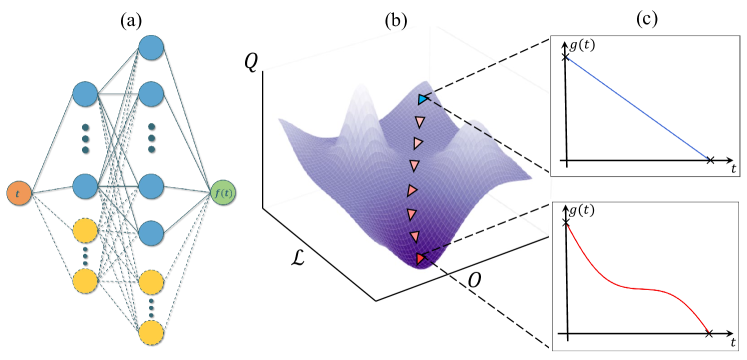
The workflow of the DCNN is illustrated in Fig. 1. The neural network has two hidden layers with units in the first layer and in the second. The parameters of the neural network can be randomly initialized. For simplicity, the parameters can be initialized by training the neural network based on the empirical form of the control field. We then add neurons to the first hidden layers and add to the second. The corresponding parameters of the newly added neurons should be randomly initialized based on the average distribution. The input of the DCNN is and the output is the following specific function
| (11) |
where are weight matrices, are bias matrices, and is the function acting on each elements of the matrix. The output undergoes a linear transformation to produce the control fields . Interestingly, increasing the number of neurons within the neural-network-based approach exhibits a conceptual parallel in model space expansion, akin to the methods employed in traditional optimal control that augment the number of optimization parameters [87, 88]. Nevertheless, the DCNN adaptively and flexibly explores model space, unlike the traditional optimal control method that enhances it by requiring prior knowledge and specific basis functions. The DCNN employs a pareto-optimization-based strategy, adeptly balancing multiple objectives without compromising any particular target. Due to the flexible optimization strategy of the DCNN, we can impose desired constraints on the form of the control field. In our work, the control field has fixed values for initial moment and final moment , which can be evaluated using the loss function
| (12) |
where and are the fixed points of for and , respectively. The other constraint, involving the extremum of the final expectation value of a specific observable .
The DCNN is capable of conducting the optimization for multiple objectives, aligning with approaches in quantum optimal control [89]. To be specific, the classical approach to solve a multi-objective optimization problem is to assign a weight to each normalized objective function so that the problem is converted to a single objective problem with a scalar objective function [90]. In our approach, the objective function is not necessarily normalized. We set to be , where and are two arbitrary real numbers. Notably, the normalization of the individual objective functions is not imperative, given the adaptability provided by the adjustable coefficients ( = 1 , 2). In order to obtain the minimum value of , we adopt the gradient descent algorithm to update all parameters,
| (13) |
for the next variation. Here, the learning rates and are adjustable parameters depending on the impact of the corresponding parameters on .
The gradients of the and with respect to all the parameters are given by
| (14) |
and
The gradients of with respect to its parameters are calculated using the chain rule and are then normalized to mitigate the risk of gradient explosion.
We only update the corresponding parameters of the newly increased neurons according to Eq. (13), while keep the other parameters unchanged. Next, if both the observable and the loss , calculated using the updated parameters, are comparatively smaller than those obtained from the original parameters, we will accept the new neurons as part of the neural network, namely, and . Otherwise, the newly introduced units are reinitialized randomly. We can iterate through the aforementioned steps to obtain the desired control field. Adding more neurons into neural network architectures involves directly with the efficiency and scalability of the model, presenting numerical cost as an interesting aspect that warrants further study [91]. While it is challenging to provide a comprehensive overview due to the complicate interplay between model complexity and computational resources, the current insights suggest that computational time and memory requirements tend to scale nearly linearly with the number of parameters (See more details in appendix B). It is also important to note that, in order to prevent the neural network from getting trapped in potential local minima, we can establish a criterion for the neural network to adjust its architecture after an extended period. Furthermore, we may approve the update even if the observable or the loss , calculated using the updated parameters, is slightly higher than those computed with the original parameters.
III Optimal suppression of defect generation in the quantum Ising model
III.1 Quantum Ising chain and gradient of the observable
In this following, we will concretely apply the DCNN method to physical scenarios, specifically focusing on enhancing the suppression of defect generation and improving the preparation of cat-states during the passage across the QCP of the 1D quantum Ising model. For the sake of numerical simplicity, we employ periodic boundary conditions for the spin chain [40, 43]. While certain local observables, i.e., local longitudinal magnetization, may differ between periodic and open boundary conditions [92], it is expected that the global observables, such as defect density and cat-state fidelity, will demonstrate analogous behavior irrespective of the boundary conditions. The Hamiltonian of a periodic quantum Ising chain with , is given by
| (15) |
where is a global transverse magnetic field that we aim to control, and for simplicity, we assume to be even. This model exhibits a quantum phase transition at between the ferromagnetic phase for and the paramagnetic phase for .
The Hamiltonian can be diagonalized through a standard procedure, which involves applying the Jordan-Wigner transformation followed by the Fourier transformation on the fermionic operators. In this study, we are interested in dynamical protocols starting from the paramagnetic phase with , ensuring that only the subspace with an even fermion number parity is pertinent [93], yielding
| (20) |
where and the ’s are fermionic operators satisfying and . Note that for open boundary conditions, the necessary adjustment to the momentum set involves solving the corresponding transcendental equation [94]. The ground and excitation states of the mode Hamiltonian are given by
| (22) |
where is the vacuum state of and . The angle is determined by , where is the single-particle dispersion with which one has and . In the present problem, the operator gives
| (23) |
Defects or domain walls will be inevitably produced during the transition from the paramagnetic phase to the ferromagnetic phase. The number of defects is measured by the operator
| (24) |
where is represented by the corresponding matrix form
| (25) |
in the two-dimensional space spanned by . According to Eq. (II.2), the gradient of with respect to is
| (26) | |||||
III.2 DCNN guided by the final defect density
We consider a quench from to within the time interval . We focus on a power-law quench characterized by the function , which has been demonstrated to effectively reduce the final defect density, defined as [65]. Notably, this power-law quench strategy surpasses the conventional linear quench [40], the assisted adiabatic passage [43] and the local adiabatic evolution approach [95] in minimizing . To test the DCNN method, we firstly consider the case of and . In the initial neural network, there are two hidden layers with neurons in the first layer and neurons in the second layer. To improve the learning efficiency of the neural network, we employ pre-training based on a gradient-oriented power-law quench to establish the initial parameters. We then set and . These values are adaptable and can be increased throughout the learning process. The parameters for the newly added neurons in these layers are randomly initialized, following a uniform distribution ranging from to . We set the learning rates to be for and . Due to the significant impact of on the , the learning rate of is set at a value tenfold higher than that of the other parameters. The weights assigned to are and , and we ensure the normalization of gradients throughout the learning process.
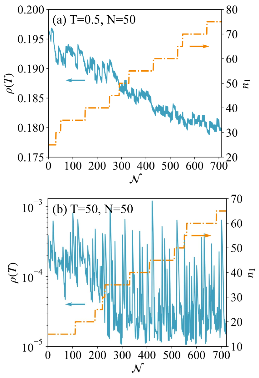
The learning results of the DCNN for and are shown in Fig. 2. The number of neurons in the first layer exhibits a stepwise increase during the learning process. Each step signifies a transformation in the neural network’s scale, leading to an enlargement of the model’s representational space. During these steps, new nodes are introduced with different initializations. The primary objective of this process is to incrementally decrease the value of through successive modifications of facilitated by these additional nodes. The interplay between reducing the final defect density and the system’s evolution through two fixed points presents an intriguing scenario. In certain cases, reducing may result in the control field diverging more substantially from these fixed points. To accelerate the convergence rate of the neural networks, we will selectively abandon the optimized form of the control field, although the trade-off could potentially become less pronounced as the neural network’s learning process advances. In this context, the DCNN exhibits a pronounced ability to navigate multiple objectives and thereby effectively mitigates oscillatory behaviors between competing objectives, fostering a more rapid convergence. In Fig. 2, we observe an oscillatory decrease in with increasing learning iteration number , indicating significant modifications to the neural network due to the introduction of additional modes. Note that outliers resulting from significant modifications in the learning process should not be a concern, as the optimization strategy automatically discards these values. As the learning process progresses in both scenarios, eventually exhibits convergence with minimal fluctuations. Specifically, converges to a finite value for , while for it stabilizes around a minimal value.
III.3 Numerical results and discussions
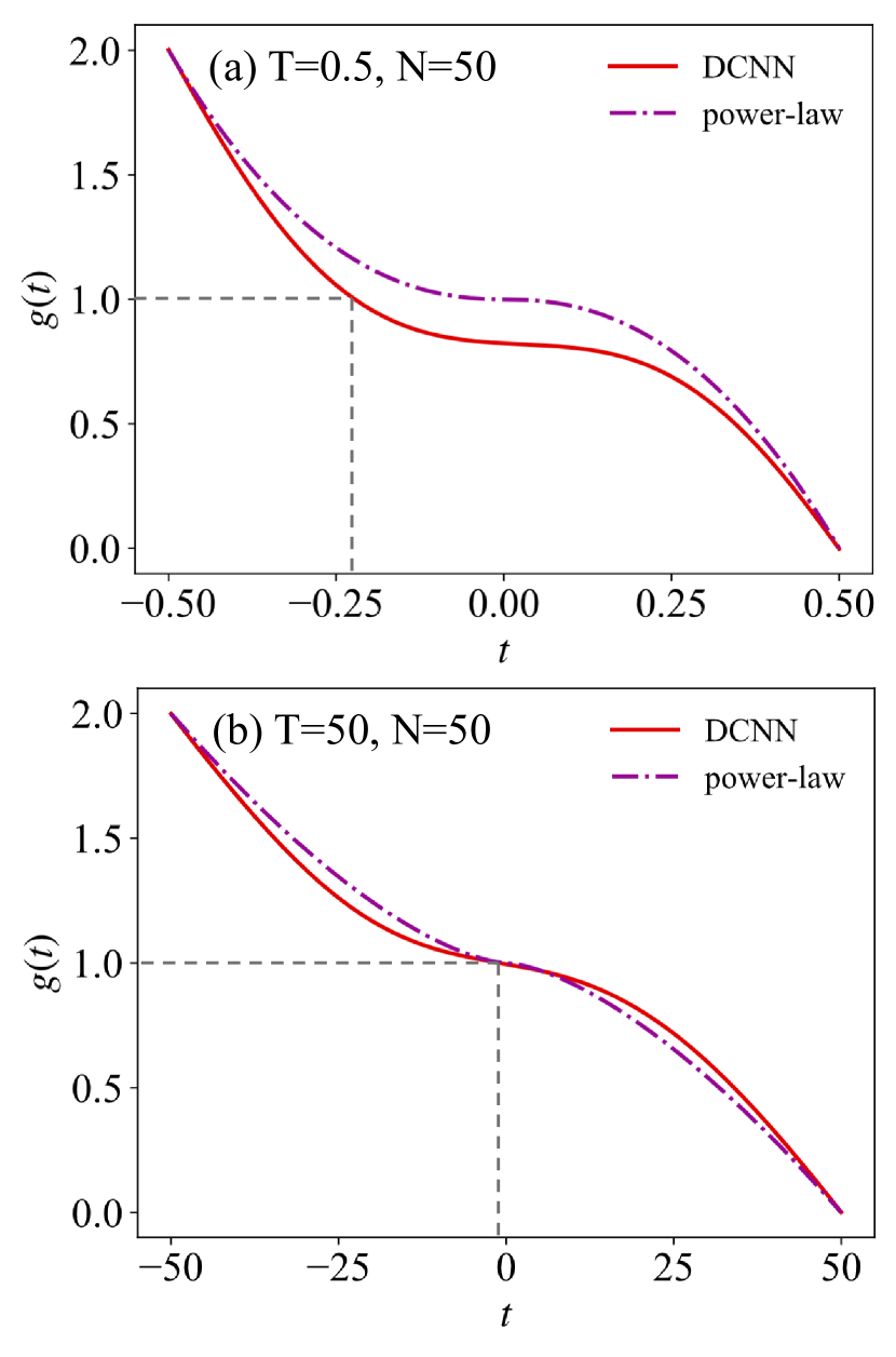
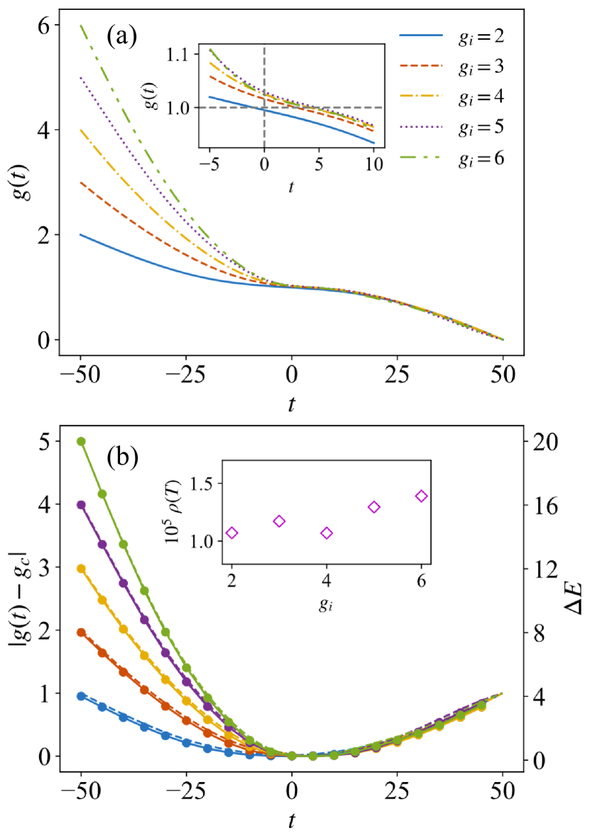
In Fig. 3, we present the optimized control field obtained by both the DCNN method and the gradient-based power-law quench. In contrast to the power-law control, the resulting lacks symmetric structure and passes through the QCP at a specific time . Interestingly, we observe that tends to increase as increases. For the long-term evolution, it remains imperative to navigate through the QCP as slowly as feasible. Nevertheless, in both instances, the slowest rate of change in occurs at . These characteristics of could provide insights into the optimal timing and approach for traversing the critical point, thereby minimizing defect generation in practical pulse design applications. Furthermore, such insights may hold the potential for generalization to state preparation protocols across various quantum critical systems.
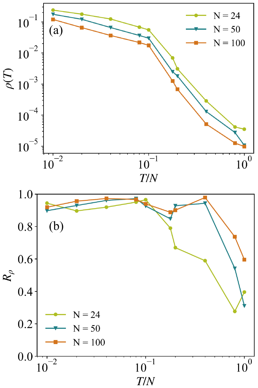
The optimized final defect density using the DCNN is plotted in Fig. 4(a) for various system sizes with ranging from 0.01 to 1. To assess the relative effectiveness of different optimization methods, we plot in Fig. 4(b) the ratio of the defect density optimized by the DCNN to that achieved through the gradient-based power-law quench. We see that the DCNN outperforms the optimal power-law quench across a broad range of parameters, particularly for small-sized systems and in the long-duration limit. Similar to the case of the optimal power-law profile, we observe a crossover in the scaled time beyond which the optimized defect density undergoes a sharp decline. The simultaneous occurrence of this crossover for different values of and suggests that the crossover time is proportional to , contrasting with the Kibble-Zurek scale for the linear quench, where scales as [40]. This occurrence can be ascribed to the implications of the quantum speed limit, which establishes a connection between the maximum speed of evolution and the system’s energy uncertainty and mean energy. Prior studies suggest that the quantum evolution in a many-body model primarily involves two lowest states in the scenario of small excitations [96, 97, 98]. This enables effective mapping into two-level Hamiltonians [99, 100, 101, 102]. In the even subspace of mode in the 1D transverse Ising model, the mode Hamiltonian in Eq. (LABEL:eq:Hk) can be reformulated in a Landau-Zener-type form as with and . There exists an intrinsic quantum speed limit to drive a general initial state to a final desired state [51], expressed by
For the quench with in the present scenario, the lowest mode specified by yields or for sufficiently large , serving as a lower bound for for the entire system, considering all modes .
The gradient-based power-law quench method, which depends on a specific power-law scheme to pass through fixed points, faces limitations in adaptability across varied initial and final state scenarios. This limitation is particularly pronounced when these states do not exhibit symmetry relative to the critical point, thereby complicating the determination of a suitable power-law function. In contrast, the DCNN offers a more adaptable framework, enabling more straightforward modifications to its optimization strategy. This adaptability suggests that the DCNN approach may provide more nuanced and flexible solutions compared to the gradient-based power-law quench method, especially regarding its application across diverse quenching scenarios. We plot the optimized control fields with different initial values of in Fig. 5 (a) for and . It is evident that smoothly passes through the QCP at some around at a relatively slow pace. As increases while keeping constant, mitigating non-adiabatic effects within a finite duration becomes challenging. The optimized control fields strikes a balance between a deliberate traversal of the QCP and avoiding excessive speed in other regions [39]. To investigate the role of the lowest mode in the optimization process, we plot the absolute value of the relative offset of to and the energy gap in Fig. 5 (b). One finds a discernible correlation between the deviation of from and the energy gap associated with the lowest mode, encapsulated by the approximate relation .
To explore potential applications, we assess the robustness of our protocol to spin number fluctuations [50], considering cases with and as examples. In experimental implementations, it is inevitable to encounter discrepancies in the actual number of spins present in the system. We thus introduce a number fluctuation parameter, . The final defect density remains below for and below for , indicating the robustness of our proposal against spin number fluctuations. To delve deeper into the effects of random noise, we examine the additive white Gaussian noise model, denoted as . We incorporate it into the control field using the relation:
| (27) |
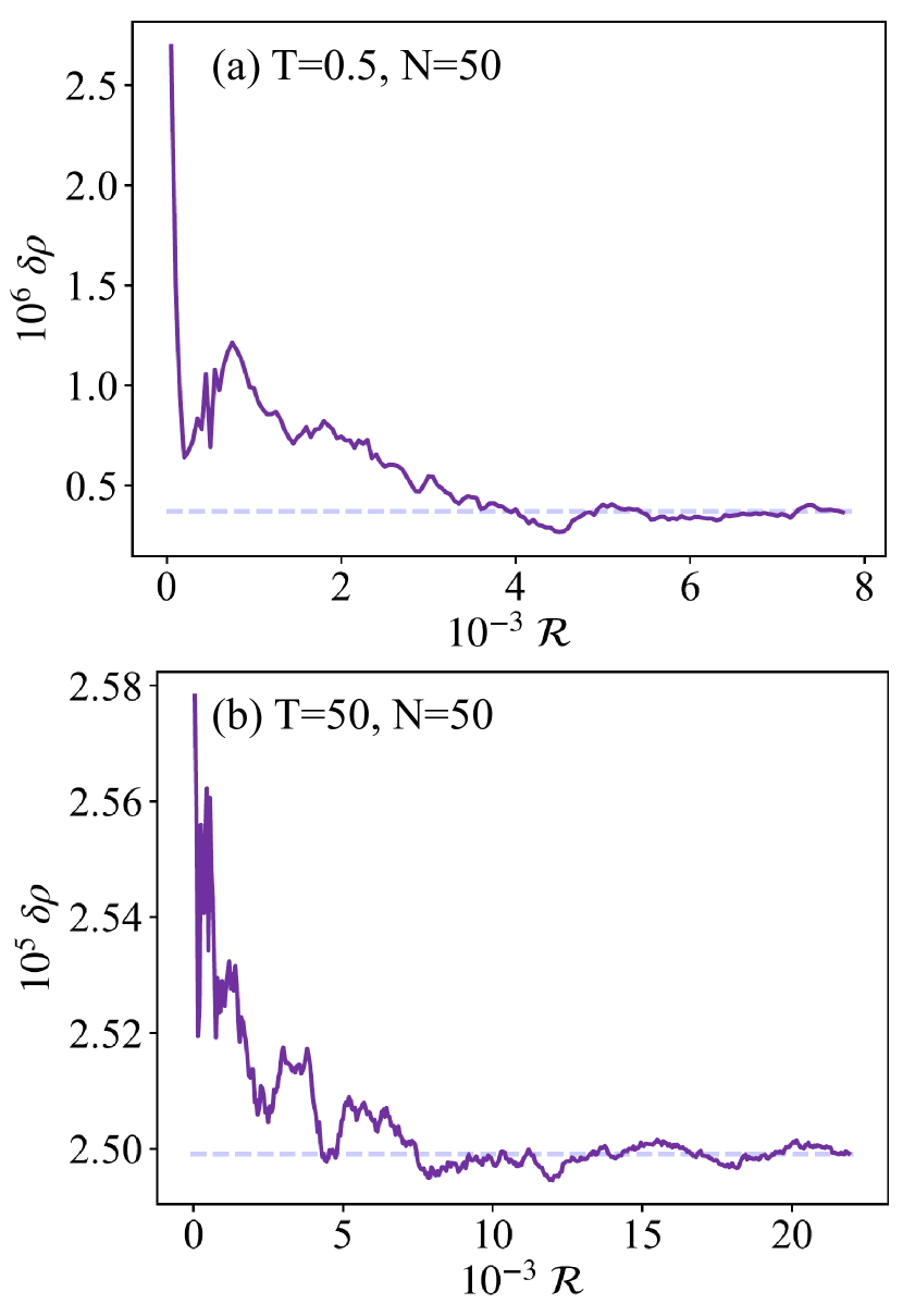
where represents each random generator , with , where and are the power of signal and noise, respectively. We evaluate our protocol’s robustness against white Gaussian noise by analyzing the mean relative offsets, , from the ideal defect densities, conducting numerical simulations with for and . Fig. 6 depicts versus , where is the simulation index, showing convergence of defect densities to and 0.1798 for the respective cases. These results highlight our scheme exhibits a high degree of robustness against random noise.
IV Optimal cat-state preparation in the quantum Ising model
In this section, we employ the DCNN to tackle a more complex task: optimally preparing a cat state in the quantum Ising chain. The Schrödinger cat states have attracted much attention from researchers due to their fundamental implications. The quantum superpositions of two macroscopically distinct states are not only interesting for testing the fundamentals of quantum mechanics such as the quantum-to-classical transition [103, 104], but also a valuable resource for quantum information processing [105, 106, 107]. Noteworthy examples of maximally entangled cat states include the NOON state [108] and Greenberger-Horne-Zeilinger (GHZ) state [109], which can push the estimation precision to the Heisenberg limit [110, 111, 112]. Of particular interest are spin cat states for use in atomic clocks [113] and magnetometers [114] due to the potential applications in diverse fields from materials science to medical diagnostics [115]. However, the realization of cat states in practical experiments faces challenges due to their sensitivity to decoherence and the delicate entanglement properties [116].
The target state we aim to achieve is
| (28) |
which is an equally weighted superposition of the two degenerate fully polarized states and . Our goal is to identify an optimized function that maximizes the final fidelity, defined as
| (29) |
It is important to note that maximizing this fidelity poses a more stringent requirement than simply minimizing the final defect density. This is because any linear combination of and would result in vanishing defects.
It is shown in Ref. [93] that can be written in the momentum space as a product state
| (30) |
with . Therefore, is actually the expectation value of the operator in the final state . From Eq. (10), the dependence of with respect to is delineated as
| (31) | |||||
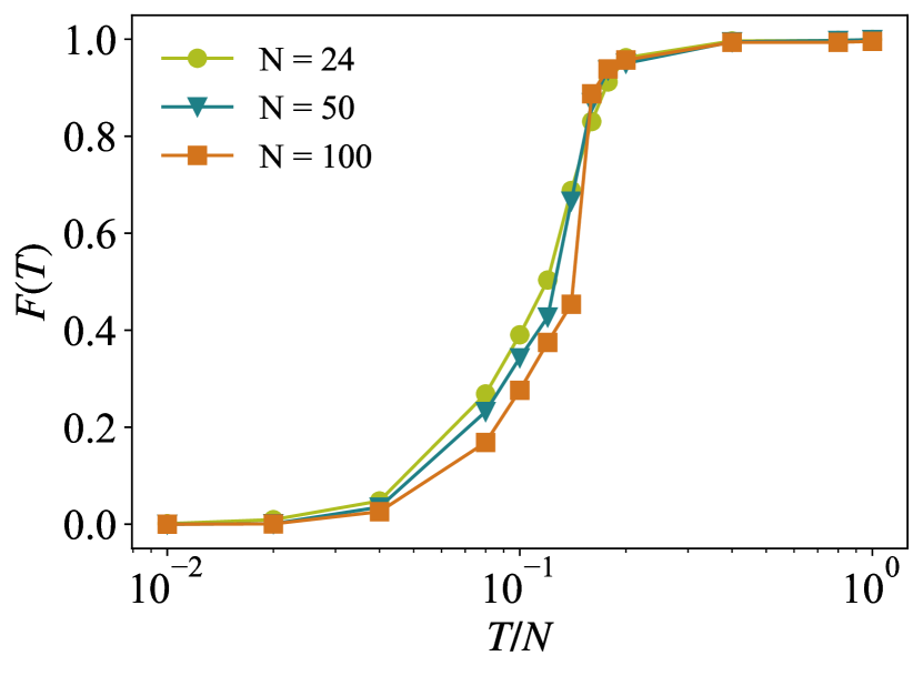
Within the DCNN framework, we also examine the quench from to over the time interval . The objective function is . The update of all parameters given by Eq. (13) will undergo corresponding adjustments to reflect changes in . The optimized fidelity results obtained through the DCNN for sizes and the ratio ranging from 0.01 to 1 are presented in Fig. 7. As expected, the achieved fidelity increases as the duration increases and approaches unity for larger . In the intermediate quench time range, specifically between , a notable surge in is observed, which is accompanied by a marked decrease in final defect density, as illustrated in Fig. 4. It is noteworthy that this rise in becomes more pronounced with the increase in system size. For shorter durations, the fidelity always remains extremely low, a consequence of the inherent constraints imposed by the quantum speed limit.
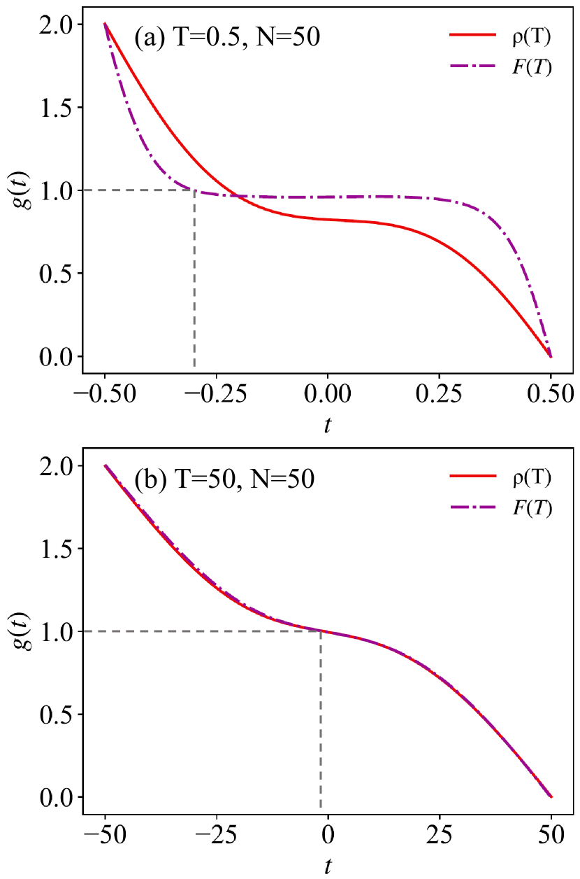
Fig. 8 displays the optimized control fields , obtained either by maximizing cat-state fidelity or by minimizing final defect density . In Fig. 8(a), a notable difference is observed between the two control fields for short durations. Specifically, the that minimizes final defect density leads to considerably lower fidelity. Conversely, for longer durations, the two profiles are nearly identical in Fig. 8(b), with each leading to either very low final defect density or significantly high fidelity. This observation implies a complex relationship between final defect density and state fidelity, indicating that they are not straightforwardly correlated.
V Conclusion and outlook
In this study, we introduce a dynamic control neural network (DCNN) approach to suppress the final defect density during a passage across a quantum critical point (QCP). Utilizing the dynamic architecture of the neural network combined with a strategic control mechanism, we successfully generate control fields that navigate through two fixed points while optimizing the desired objective. By considering various evolution time and system sizes , our method achieves a lower final defect density compared to traditional gradient-based power-law quench methods. Meanwhile, our study reveals that the optimized final defect density undergoes a crossover at a specific critical ratio of quench duration to system size. This transition closely aligns with the quantum speed limit for evolution, which is profoundly influenced by the lowest mode. We numerically demonstrate that our protocol is robust against the random noise and the spin number fluctuations. Additionally, we demonstrate the effectiveness of our method using control fields that are optimized across a range of initial values. By analyzing variational control field forms and comparing them to power-law quench methods, we offer insights for experimental pulse design. The versatility of the DCNN is further highlighted by its application to enhancing cat-state fidelity, providing similar optimized solutions indicative of the quantum speed limit. Our findings reveal a non-one-to-one correspondence between final defect density and fidelity. To attain high-quality quantum many-body states, it is crucial to exceed the critical ratio of quench duration to system size.
Noting that the DCNN method introduced in this study extends beyond the preparation of spin cat states, holding promise for a broad range of applications in quantum technologies. With the rapid advancements in quantum computation [117, 118, 119, 120] and quantum metrology [121, 122, 123, 124], the DCNN’s capability for optimizing complex quantum systems positions it as a valuable tool for enhancing precision in quantum information science. The application of the DCNN method to multi-objective optimization in quantum control demonstrates its potential applicability, especially in complex scenarios such as quantum many-body systems and open quantum systems.
Acknowledgements.
This work is supported by the National Natural Science Foundation of China (NSFC) under Grant No. 12174194 and stable supports for basic institute research under Grant No. 190101. N. W. was supported by the National Key Research and Development Program of China under Grant No. 2021YFA1400803.Appendix A The gradients of with respect to
The gradients of the final expectation value with respect to the control field can be written as
| (32) |
where
| (33) | |||||
Combining Eq. (32) with Eq. (33), we derive the following expression:
| (34) |
For simplicity, the is abbreviated as . We have assumed that the control term can be expressed as a summation over even operators of independent mode . If can be represented as a sum of even operators over independent modes, such that , then it follows that:
| (35) | |||||
In deriving the penultimate line of Eq. (35), we have used the identity
| (36) |
Then, we can obtain Eq. (II.2). If can be expressed as a product over even operators of independent modes , it can be calculated as
| (37) | |||||
We also use the identity in Eq.(36) in the above derivation.
Appendix B The numerical cost in neural network expansion
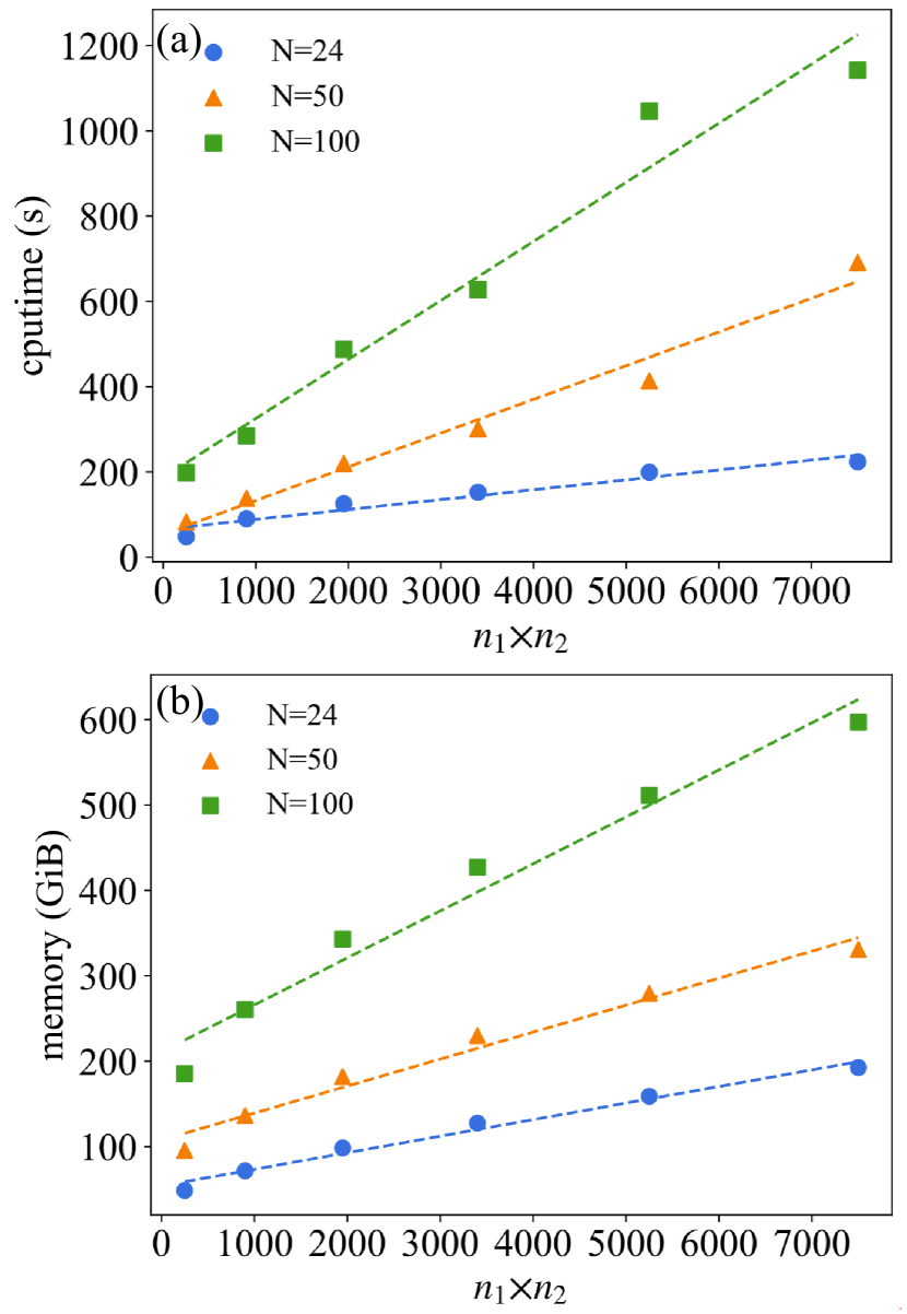
The parameter scale of expanding a DCNN can be quantified as , where represents the number of expanding the neural network as the network approaches convergence. For an intuitive understanding, when the initial network size is substantially smaller than , the parameter growth simplifies to . Conversely, for an initially larger network relative to , the complexity remains closer to . For simplicity, we only consider the computational time and the memory consumption of increasing the neurons one time, transitioning the network from an to an structure. where denotes a network with neurons in the first and in the second hidden layers, respectively. The overall impact on computational time and memory can be approximated by , with representing the number of iterations until successful neuron integration, and capturing the associated time or memory costs. It’s noteworthy that computational duration is subject to a variety of external factors, including CPU performance and specific elements of the matrix. Assuming a constant spin length, the variation in numerical costs linked to different network sizes is illustrated in Fig. 9. With the parameter scale increases, we observe an almost linear surge in computational time, indicative of the added complexity and data processing requirements. Memory usage similarly rises, though its growth trajectory is shallower compared to computational time, which suggests a higher data throughput and computational complexity for larger networks. An extension in spin length further accentuates these resource demands. However, a quantifiable relationship between network size expansion and computational resource consumption requires further investigation.
References
- Farhi et al. [2001] E. Farhi, J. Goldstone, S. Gutmann, J. Lapan, A. Lundgren, and D. Preda, Science 292, 472 (2001).
- Chen et al. [2009] X. Chen, B. Zeng, Z.-C. Gu, B. Yoshida, and I. L. Chuang, Phys. Rev. Lett. 102, 220501 (2009).
- Verstraete et al. [2004] F. Verstraete, J. J. García-Ripoll, and J. I. Cirac, Phys. Rev. Lett. 93, 207204 (2004).
- Sørensen et al. [2010] A. S. Sørensen, E. Altman, M. Gullans, J. V. Porto, M. D. Lukin, and E. Demler, Phys. Rev. A 81, 061603 (2010).
- Ljubotina et al. [2022] M. Ljubotina, B. Roos, D. A. Abanin, and M. Serbyn, PRX Quantum 3, 030343 (2022).
- Shettell and Markham [2020] N. Shettell and D. Markham, Phys. Rev. Lett. 124, 110502 (2020).
- Frérot and Roscilde [2018] I. Frérot and T. Roscilde, Phys. Rev. Lett. 121, 020402 (2018).
- Altherr and Yang [2021] A. Altherr and Y. Yang, Phys. Rev. Lett. 127, 060501 (2021).
- Kessler et al. [2014] E. M. Kessler, I. Lovchinsky, A. O. Sushkov, and M. D. Lukin, Phys. Rev. Lett. 112, 150802 (2014).
- Hudelist et al. [2014] F. Hudelist, J. Kong, C. Liu, J. Jing, Z. Ou, and W. Zhang, Nature Communications 5, 3049 (2014).
- Marciniak et al. [2022] C. D. Marciniak, T. Feldker, I. Pogorelov, R. Kaubruegger, D. V. Vasilyev, R. van Bijnen, P. Schindler, P. Zoller, R. Blatt, and T. Monz, Nature 603, 604 (2022).
- Yin et al. [2023] P. Yin, X. Zhao, Y. Yang, Y. Guo, W.-H. Zhang, G.-C. Li, Y.-J. Han, B.-H. Liu, J.-S. Xu, G. Chiribella, G. Chen, C.-F. Li, and G.-C. Guo, Nature Physics 19, 1122 (2023).
- Tóth and Apellaniz [2014] G. Tóth and I. Apellaniz, Journal of Physics A: Mathematical and Theoretical 47, 424006 (2014).
- Szigeti et al. [2021] S. S. Szigeti, O. Hosten, and S. A. Haine, Applied Physics Letters 118, 140501 (2021).
- Giovannetti et al. [2004] V. Giovannetti, S. Lloyd, and L. Maccone, Science 306, 1330 (2004).
- Giovannetti et al. [2011] V. Giovannetti, S. Lloyd, and L. Maccone, Nature Photonics 5, 222 (2011).
- Huang et al. [2014] J. Huang, S. Wu, H. Zhong, and C. Lee, Annual Review of Cold Atoms and Molecules , 365 (2014).
- Zhang et al. [2019] C. Zhang, T. R. Bromley, Y.-F. Huang, H. Cao, W.-M. Lv, B.-H. Liu, C.-F. Li, G.-C. Guo, M. Cianciaruso, and G. Adesso, Phys. Rev. Lett. 123, 180504 (2019).
- Giorda and Paris [2010] P. Giorda and M. G. A. Paris, Phys. Rev. Lett. 105, 020503 (2010).
- Ollivier and Zurek [2001] H. Ollivier and W. H. Zurek, Phys. Rev. Lett. 88, 017901 (2001).
- Note [1] If there are qubits in separable states, it is known that the uncertainty (that is, the inverse of the sensitivity) scales as , which is called the standard quantum limit, while quantum physics allows the ultimate scalings being , i.e., the Heisenberg scaling, in the absence of noise and in the presence of realistic decoherence.
- Chu and Cai [2022] Y. Chu and J. Cai, Phys. Rev. Lett. 128, 200501 (2022).
- Lücke et al. [2011] B. Lücke, M. Scherer, J. Kruse, L. Pezzé, F. Deuretzbacher, P. Hyllus, O. Topic, J. Peise, W. Ertmer, J. Arlt, L. Santos, A. Smerzi, and C. Klempt, Science 334, 773 (2011).
- Strobel et al. [2014] H. Strobel, W. Muessel, D. Linnemann, T. Zibold, D. B. Hume, L. Pezzè, A. Smerzi, and M. K. Oberthaler, Science 345, 424 (2014).
- Rahmani and Chamon [2011] A. Rahmani and C. Chamon, Phys. Rev. Lett. 107, 016402 (2011).
- Zaletel et al. [2021] M. P. Zaletel, A. Kaufman, D. M. Stamper-Kurn, and N. Y. Yao, Phys. Rev. Lett. 126, 103401 (2021).
- Farooq et al. [2015] U. Farooq, A. Bayat, S. Mancini, and S. Bose, Phys. Rev. B 91, 134303 (2015).
- Reiter et al. [2016] F. Reiter, D. Reeb, and A. S. Sørensen, Phys. Rev. Lett. 117, 040501 (2016).
- Wei et al. [2023] Z.-Y. Wei, D. Malz, and J. I. Cirac, Phys. Rev. Res. 5, L022037 (2023).
- Motta et al. [2020] M. Motta, C. Sun, A. T. K. Tan, M. J. O’Rourke, E. Ye, A. J. Minnich, F. G. S. L. Brandão, and G. K.-L. Chan, Nature Physics 16, 205 (2020).
- Choi et al. [2023] J. Choi, A. L. Shaw, I. S. Madjarov, X. Xie, R. Finkelstein, J. P. Covey, J. S. Cotler, D. K. Mark, H.-Y. Huang, A. Kale, H. Pichler, F. G. S. L. Brandão, S. Choi, and M. Endres, Nature 613, 468 (2023).
- Léonard et al. [2023] J. Léonard, S. Kim, J. Kwan, P. Segura, F. Grusdt, C. Repellin, N. Goldman, and M. Greiner, Nature 619, 495 (2023).
- Bernien et al. [2017] H. Bernien, S. Schwartz, A. Keesling, H. Levine, A. Omran, H. Pichler, S. Choi, A. S. Zibrov, M. Endres, M. Greiner, V. Vuletić, and M. D. Lukin, Nature 551, 579 (2017).
- Maslova et al. [2019] N. S. Maslova, P. I. Arseyev, and V. N. Mantsevich, Scientific Reports 9, 3130 (2019).
- Kato [1950] T. Kato, Journal of the Physical Society of Japan 5, 435 (1950).
- Tabatabaei et al. [2021] S. Tabatabaei, H. Haas, W. Rose, B. Yager, M. Piscitelli, P. Sahafi, A. Jordan, P. J. Poole, D. Dalacu, and R. Budakian, Phys. Rev. Appl. 15, 044043 (2021).
- Xiang-Bin and Keiji [2001] W. Xiang-Bin and M. Keiji, Phys. Rev. Lett. 87, 097901 (2001).
- Dziarmaga [2010] J. Dziarmaga, Advances in Physics 59, 1063 (2010).
- Barankov and Polkovnikov [2008] R. Barankov and A. Polkovnikov, Phys. Rev. Lett. 101, 076801 (2008).
- Dziarmaga [2005] J. Dziarmaga, Phys. Rev. Lett. 95, 245701 (2005).
- Jozsa [1994] R. Jozsa, Journal of Modern Optics 41, 2315 (1994).
- Nielsen and Chuang [2010] M. A. Nielsen and I. Chuang, Quantum computation and quantum information (Cambridge University Press, 2010).
- del Campo et al. [2012] A. del Campo, M. M. Rams, and W. H. Zurek, Phys. Rev. Lett. 109, 115703 (2012).
- Sau and Sengupta [2014] J. D. Sau and K. Sengupta, Phys. Rev. B 90, 104306 (2014).
- Damski [2014] B. Damski, Journal of Statistical Mechanics: Theory and Experiment 2014, P12019 (2014).
- Deffner et al. [2014] S. Deffner, C. Jarzynski, and A. del Campo, Phys. Rev. X 4, 021013 (2014).
- Campbell et al. [2015] S. Campbell, G. De Chiara, M. Paternostro, G. M. Palma, and R. Fazio, Phys. Rev. Lett. 114, 177206 (2015).
- Guéry-Odelin et al. [2019] D. Guéry-Odelin, A. Ruschhaupt, A. Kiely, E. Torrontegui, S. Martínez-Garaot, and J. G. Muga, Rev. Mod. Phys. 91, 045001 (2019).
- Koch et al. [2022] C. P. Koch, U. Boscain, T. Calarco, G. Dirr, S. Filipp, S. J. Glaser, R. Kosloff, S. Montangero, T. Schulte-Herbrüggen, D. Sugny, and F. K. Wilhelm, EPJ Quantum Technology 9, 19 (2022).
- Doria et al. [2011] P. Doria, T. Calarco, and S. Montangero, Phys. Rev. Lett. 106, 190501 (2011).
- Hegerfeldt [2013] G. C. Hegerfeldt, Phys. Rev. Lett. 111, 260501 (2013).
- Caneva et al. [2009] T. Caneva, M. Murphy, T. Calarco, R. Fazio, S. Montangero, V. Giovannetti, and G. E. Santoro, Phys. Rev. Lett. 103, 240501 (2009).
- Giannelli et al. [2022] L. Giannelli, S. Sgroi, J. Brown, G. S. Paraoanu, M. Paternostro, E. Paladino, and G. Falci, Physics Letters A 434, 128054 (2022).
- Giovannetti et al. [2003] V. Giovannetti, S. Lloyd, and L. Maccone, Phys. Rev. A 67, 052109 (2003).
- Levitin and Toffoli [2009] L. B. Levitin and T. Toffoli, Phys. Rev. Lett. 103, 160502 (2009).
- Deffner and Campbell [2017] S. Deffner and S. Campbell, Journal of Physics A: Mathematical and Theoretical 50, 453001 (2017).
- Bukov et al. [2019] M. Bukov, D. Sels, and A. Polkovnikov, Phys. Rev. X 9, 011034 (2019).
- Zhang et al. [2023] M. Zhang, H.-M. Yu, and J. Liu, npj Quantum Information 9, 97 (2023).
- Carleo and Troyer [2017] G. Carleo and M. Troyer, Science 355, 602 (2017).
- Choo et al. [2018] K. Choo, G. Carleo, N. Regnault, and T. Neupert, Phys. Rev. Lett. 121, 167204 (2018).
- Choo et al. [2020] K. Choo, A. Mezzacapo, and G. Carleo, Nature Communications 11, 2368 (2020).
- Zhu et al. [2022] Y. Zhu, Y.-D. Wu, G. Bai, D.-S. Wang, Y. Wang, and G. Chiribella, Nature Communications 13, 6222 (2022).
- Carleo et al. [2018] G. Carleo, Y. Nomura, and M. Imada, Nature Communications 9, 5322 (2018).
- Day et al. [2019] A. G. R. Day, M. Bukov, P. Weinberg, P. Mehta, and D. Sels, Phys. Rev. Lett. 122, 020601 (2019).
- Wu et al. [2015] N. Wu, A. Nanduri, and H. Rabitz, Phys. Rev. B 91, 041115 (2015).
- Mi et al. [2022a] X. Mi, M. Ippoliti, C. Quintana, A. Greene, Z. Chen, J. Gross, F. Arute, K. Arya, J. Atalaya, et al., Nature 601, 531 (2022a).
- Frey and Rachel [2022] P. Frey and S. Rachel, Science Advances 8, eabm7652 (2022).
- Chen et al. [2022] I.-C. Chen, B. Burdick, Y. Yao, P. P. Orth, and T. Iadecola, Phys. Rev. Res. 4, 043027 (2022).
- Mi et al. [2022b] X. Mi, M. Sonner, M. Y. Niu, K. W. Lee, B. Foxen, R. Acharya, I. Aleiner, T. I. Andersen, F. Arute, et al., Science 378, 785 (2022b).
- Turner et al. [2018] C. J. Turner, A. A. Michailidis, D. A. Abanin, M. Serbyn, and Z. Papić, Phys. Rev. B 98, 155134 (2018).
- Wild et al. [2021] D. S. Wild, D. Sels, H. Pichler, C. Zanoci, and M. D. Lukin, Phys. Rev. Lett. 127, 100504 (2021).
- Bravyi et al. [2020] S. Bravyi, A. Kliesch, R. Koenig, and E. Tang, Phys. Rev. Lett. 125, 260505 (2020).
- Kairys et al. [2020] P. Kairys, A. D. King, I. Ozfidan, K. Boothby, J. Raymond, A. Banerjee, and T. S. Humble, PRX Quantum 1, 020320 (2020).
- Schiffer et al. [2022] B. F. Schiffer, J. Tura, and J. I. Cirac, PRX Quantum 3, 020347 (2022).
- Zhang et al. [2021] D.-B. Zhang, G.-Q. Zhang, Z.-Y. Xue, S.-L. Zhu, and Z. D. Wang, Phys. Rev. Lett. 127, 020502 (2021).
- Kraus [2011] B. Kraus, Phys. Rev. Lett. 107, 250503 (2011).
- Schauss [2018] P. Schauss, Quantum Science and Technology 3, 023001 (2018).
- Kim et al. [2010] K. Kim, M.-S. Chang, S. Korenblit, R. Islam, E. E. Edwards, J. K. Freericks, G.-D. Lin, L.-M. Duan, and C. Monroe, Nature 465, 590 (2010).
- Mostame and Schützhold [2008] S. Mostame and R. Schützhold, Phys. Rev. Lett. 101, 220501 (2008).
- Cervera-Lierta [2018] A. Cervera-Lierta, Quantum 2, 114 (2018).
- Kim et al. [2023] Y. Kim, A. Eddins, S. Anand, K. X. Wei, E. van den Berg, S. Rosenblatt, H. Nayfeh, Y. Wu, M. Zaletel, K. Temme, and A. Kandala, Nature 618, 500 (2023).
- Sachdev [1999] S. Sachdev, Physics World 12, 33 (1999).
- Kitaev [2003] A. Kitaev, Annals of Physics 303, 2 (2003).
- Wu [2012] N. Wu, Physics Letters A 376, 3530 (2012).
- Brif et al. [2010] C. Brif, R. Chakrabarti, and H. Rabitz, New Journal of Physics 12, 075008 (2010).
- Note [2] Zheng Cheng, Meng-Jiao Lyu, Takayuki Myo, Hisashi Horiuchi, Hiroshi Toki, Zhong-Zhou Ren, Masahiro Isaka, Meng-Yun Mao, Hiroki Takemoto, Niu Wan, Wen-Long You, and Qing Zhao, to appear.
- Rach et al. [2015] N. Rach, M. M. Müller, T. Calarco, and S. Montangero, Phys. Rev. A 92, 062343 (2015).
- Goetz et al. [2016] R. E. Goetz, M. Merkel, A. Karamatskou, R. Santra, and C. P. Koch, Phys. Rev. A 94, 023420 (2016).
- Chakrabarti et al. [2008] R. Chakrabarti, R. Wu, and H. Rabitz, Phys. Rev. A 78, 033414 (2008).
- Giagkiozis and Fleming [2015] I. Giagkiozis and P. Fleming, Information Sciences 293, 338 (2015).
- Huang et al. [2022a] H.-Y. Huang, R. Kueng, G. Torlai, V. V. Albert, and J. Preskill, Science 377, eabk3333 (2022a).
- Białończyk and Damski [2020] M. Białończyk and B. Damski, Journal of Statistical Mechanics: Theory and Experiment 2020, 013108 (2020).
- Wu [2020] N. Wu, Phys. Rev. E 101, 042108 (2020).
- Cabrera and Jullien [1987] G. G. Cabrera and R. Jullien, Phys. Rev. B 35, 7062 (1987).
- Roland and Cerf [2002] J. Roland and N. J. Cerf, Phys. Rev. A 65, 042308 (2002).
- Wang et al. [2020] Y. Wang, Y. Su, X. Chen, and C. Wu, Phys. Rev. Appl. 14, 044043 (2020).
- Bera et al. [2022] A. K. Bera, S. M. Yusuf, S. K. Saha, M. Kumar, D. Voneshen, Y. Skourski, and S. A. Zvyagin, Nature Communications 13, 6888 (2022).
- Wang et al. [2016] Y. Wang, J. Zhang, C. Wu, J. Q. You, and G. Romero, Phys. Rev. A 94, 012328 (2016).
- Bason et al. [2012] M. G. Bason, M. Viteau, N. Malossi, P. Huillery, E. Arimondo, D. Ciampini, R. Fazio, V. Giovannetti, R. Mannella, and O. Morsch, Nature Physics 8, 147 (2012).
- Cimmarusti et al. [2015] A. D. Cimmarusti, Z. Yan, B. D. Patterson, L. P. Corcos, L. A. Orozco, and S. Deffner, Phys. Rev. Lett. 114, 233602 (2015).
- Li [2023] X. Li, Scientific Reports 13, 14734 (2023).
- Vepsäläinen et al. [2019] A. Vepsäläinen, S. Danilin, and G. S. Paraoanu, Science Advances 5, eaau5999 (2019).
- Schrödinger [1935] E. Schrödinger, Naturwissenschaften 23, 807 (1935).
- Wineland [2013] D. J. Wineland, Rev. Mod. Phys. 85, 1103 (2013).
- Zurek [2001] W. H. Zurek, Nature 412, 712 (2001).
- Ofek et al. [2016] N. Ofek, A. Petrenko, R. Heeres, P. Reinhold, Z. Leghtas, B. Vlastakis, Y. Liu, L. Frunzio, S. M. Girvin, L. Jiang, M. Mirrahimi, M. H. Devoret, and R. J. Schoelkopf, Nature 536, 441 (2016).
- Sun et al. [2021] F.-X. Sun, S.-S. Zheng, Y. Xiao, Q. Gong, Q. He, and K. Xia, Phys. Rev. Lett. 127, 087203 (2021).
- Dowling [2008] J. P. Dowling, Contemporary Physics 49, 125 (2008).
- Huang et al. [2022b] J. Huang, H. Huo, M. Zhuang, and C. Lee, Phys. Rev. A 105, 062456 (2022b).
- Giovannetti et al. [2006] V. Giovannetti, S. Lloyd, and L. Maccone, Phys. Rev. Lett. 96, 010401 (2006).
- Lee [2006] C. Lee, Phys. Rev. Lett. 97, 150402 (2006).
- Pezzé and Smerzi [2009] L. Pezzé and A. Smerzi, Phys. Rev. Lett. 102, 100401 (2009).
- Martin et al. [2013] M. J. Martin, M. Bishof, M. D. Swallows, X. Zhang, C. Benko, J. von Stecher, A. V. Gorshkov, A. M. Rey, and J. Ye, Science 341, 632 (2013).
- Wasilewski et al. [2010] W. Wasilewski, K. Jensen, H. Krauter, J. J. Renema, M. V. Balabas, and E. S. Polzik, Phys. Rev. Lett. 104, 133601 (2010).
- Le Sage et al. [2013] D. Le Sage, K. Arai, D. R. Glenn, S. J. DeVience, L. M. Pham, L. Rahn-Lee, M. D. Lukin, A. Yacoby, A. Komeili, and R. L. Walsworth, Nature 496, 486 (2013).
- Leibfried et al. [2005] D. Leibfried, E. Knill, S. Seidelin, J. Britton, R. B. Blakestad, J. Chiaverini, D. B. Hume, W. M. Itano, J. D. Jost, C. Langer, R. Ozeri, R. Reichle, and D. J. Wineland, Nature 438, 639 (2005).
- Cesa and Pichler [2023] F. Cesa and H. Pichler, Phys. Rev. Lett. 131, 170601 (2023).
- Xia et al. [2023] J. Xia, X. Zhang, X. Liu, Y. Zhou, and M. Ezawa, Phys. Rev. Lett. 130, 106701 (2023).
- Bombín et al. [2023] H. Bombín, C. Dawson, R. V. Mishmash, N. Nickerson, F. Pastawski, and S. Roberts, PRX Quantum 4, 020303 (2023).
- Mueller et al. [2023] N. Mueller, J. A. Carolan, A. Connelly, Z. Davoudi, E. F. Dumitrescu, and K. Yeter-Aydeniz, PRX Quantum 4, 030323 (2023).
- Salvia et al. [2023] R. Salvia, M. Mehboudi, and M. Perarnau-Llobet, Phys. Rev. Lett. 130, 240803 (2023).
- Zhou et al. [2023] S. Zhou, S. Michalakis, and T. Gefen, PRX Quantum 4, 040305 (2023).
- Faist et al. [2023] P. Faist, M. P. Woods, V. V. Albert, J. M. Renes, J. Eisert, and J. Preskill, PRX Quantum 4, 040336 (2023).
- Liu et al. [2023] Q. Liu, Z. Hu, H. Yuan, and Y. Yang, Phys. Rev. Lett. 130, 070803 (2023).