All triangulations have a common stellar subdivision
Abstract.
We address two longstanding open problems, one originating in PL topology, another in birational geometry. First, we prove the weighted version of Oda’s strong factorization conjecture (1978), and prove that every two birational toric varieties are related by a common iterated blowup (at rationally smooth points). Second, we prove that every two PL homeomorphic polyhedra have a common stellar subdivisions, as conjectured by Alexander in 1930.
For Frank, in memory
1. Introduction
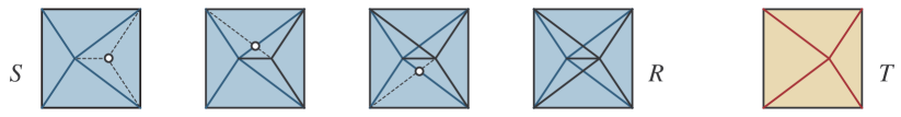
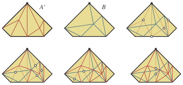
Let be a geometric complex in , and let be a triangulation of . Define a stellar subdivision at point to be a transformation given by adding to cones over all faces in containing (see Figure 3.1). We say that a triangulation can be obtained by stellar subdivisions from a triangulation , if there is a finite sequence of stellar subdivisions which start at and end with . When can be obtained by stellar subdivisions from triangulation and , it is called a common stellar subdivision (see Figure 2.1 below).
Theorem 1.1 (weighted strong factorization theorem).
Every two triangulations of a geometric complex in , have a common stellar subdivision. Moreover, if both and have coordinates in a field extension over , then so does the common stellar subdivision.
Corollary 1.2.
Every two birationally isomorphic toric varieties have a common toric blowup (with blowups at rationally smooth points).
The weak factorization conjecture states that every two triangulations of a geometric complex in are connected by a sequence of stellar subdivisions and their inverses. This was proved in dimension at most three in [Dan83], and in full generality in [Wło97], see also [A+02, IS10].
Morelli claimed the proof of the strong factorization conjecture in [Mor96], which was shown incorrect in [Mat00]. In a positive direction, the conjecture was confirmed in [Mac21] for a very special class of polyhedra. In [DK11], the authors proposed an algorithmic construction, which remains unproven (cf. 7.5). Our approach is notably different, but is also constructive. As an application, we obtain the following result.
Theorem 1.3 (former Alexander’s conjecture).
Every two PL homeomorphic simplicial complexes have combinatorially isomorphic stellar subdivisions.
Alexander [Ale30] was interested in PL homeomorphisms of polyhedral spaces, and the theorem says that every two PL homeomorphic polyhedra have a common stellar subdivision. In this case, we do not have a geometric meaning, but a topological one. In dimension , the conjecture was proved by Ewald [Ewa86]. For the context of Alexander’s conjecture, see e.g. [Lik99, 4].
2. Basic definitions and notation
Let be a polyhedral complex embedded in . We say that is a triangulation if it is simplicial. We use the same terms and notation in both geometric (realized in the Euclidean space) and topological setting (abstract complexes within the PL category), hoping this would not lead to a confusion. We use the terms “geometric triangulation”, “geometric (polyhedral) complex”, etc., when the distinction needs to be emphasized. However, until Section 6, we exclusively work in the geometric setting.
Denote by the set of triangulations of . We write if is a refinement of , where , that is, if every simplex of is contained in a simplex of . We write if can be obtained from by a sequence of stellar subdivisions. In this case we say that is an iterated stellar subdivision of . We will speak of common iterated stellar subdivision of triangulations to mean a triangulation , such that and , see Figure 2.1.
Let be a simplicial subcomplex and let be a face of . The star is the minimal simplicial subcomplex of that contains all faces containing . The link is the boundary of with respect to the intrinsic topology of . We use to denote maximal subcomplex of which does not contain , also called the antistar of in .
3. Planar case
In this and the following two sections we are concerned only with geometric triangulations. In this section, we consider triangulations of a convex polygon. In the next two sections, we consider geometric complexes in higher dimensions.
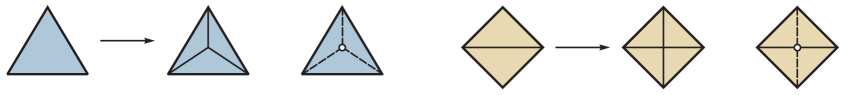
Note that in the plane, there are only two types of stellar subdivisions shown in Figure 3.1 below.111Strictly speaking, there is a third combinatorial type, when the added vertex is on the boundary. To illustrate that, simply delete the bottom triangle from the second type of stellar subdivision. The circle and dashed lines indicate the added vertices and edges. We use this notation throughout the paper (see e.g. Figure 2.1 above).
3.1. Triangulations of polygons
The case of is especially elegant since in this case a triangulation of a convex polygon in the plane is a face to face subdivision into triangles. In this section we present a self-contained proof of the weighted Oda conjecture in the plane.
Let be a convex polygon in the plane, and let be a triangulation of . Let be a point in the relative interior of a triangle in , and let be a triangulation obtained from by adding edges , and . Similarly, let be a point in the relative interior of an edge , and let be a triangulation obtained from by adding edges for all triangles in . A stellar subdivision is an operation in both cases. Clearly, we then have .
Theorem 3.1 (strong factorization for convex polygons).
Suppose triangulations of a convex polygon have at most vertices. Then there is a triangulation which can be obtained by a sequence of at most stellar subdivisions from both and .
The theorem follows from the stellar subdivision algorithm we present below.
3.2. Stellar subdivision of fins
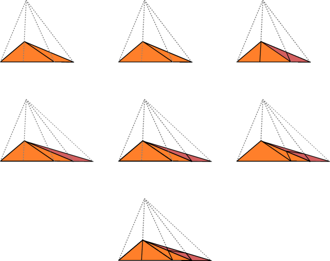
Let be a polygon in the plane, that is, a disk with polygonal boundary, and let be its set of vertices. Fix a vertex which we call an anchor.
We say that is star-shaped at anchor , if for all . We call a strictly star-shaped if for every point in , the line segment from to intersects the boundary of only in and possibly . Denote by the boundary of . For a region , denote by the restriction of triangulation to .
Let be a triangulation of a strictly star-shaped polygon . We call a fin with respect to the anchor . We say a polytope is compatible with a polyhedral complex if restricting to the faces contained in is a subdivision of .
We think of at the set of triangles, and use and to denote vertices and edges in , respectively. We say that is a scaled fin (triangulation) anchored at , if for every vertex , the triangulation is compatible with the line segment from to .
A scaled fin without interior vertices is called a stripe. We also consider the stripe associated to a fin : It is the minimal stripe containing all vertices of . An interesting case is the one when is a scaled fin, and is its stripe.
Lemma 3.2.
Let be a vertex of the polygon which is star-shaped at . Let be scaled fins of anchored at , such that and that is the stripe of . Then .
Proof.
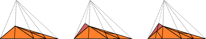
Use induction on the number of vertices in . If has no interior vertices, we have and the result is trivial. In general, suppose is an edge of such that and separates two triangles along the boundary . By going along the boundary, is easy to see that there exists at least one such edge .
There are two cases. First, suppose and separates into a triangle and a polygon . Make a stellar move in by adding the edge to obtain a triangulation of . Since is star-shaped at , this reduced the problem to triangulations and , where .
Second, suppose and separates triangles and in . Now collapse , i.e. let . Make a stellar move in by adding a vertex with edges and , to obtain a triangulation of . Since is star-shaped at , this reduced the problem to triangulations and , where .
Note that in the second case polygon can become connected in only, see Figure 3.2. This does not affect the argument, as one can treat each component separately and proceed by induction. This completes the proof. ∎
Remark 3.3.
The algorithm in the proof will be called the shedding routine. Recall that for a triangulation with vertices, the number of edges and the number of triangles . Thus, the number of stellar subdivisions used by the shedding routine is at most .
3.3. Common stellar triangulations in the plane
To construct a common stellar triangulation, follows a series of steps. Start with triangulations of a convex polygon in the plane. Fix a vertex . Let and , so .
Step 1. Use stellar subdivisions in to construct a scaled fin triangulation that is anchored at . Proceed as follows. For every vertex , let be an interval such that and . We will add such intervals one by one in any order, until the desired scaled fin is obtained.
To add , note that intersects the existing edges . Make a stellar subdivision at points of intersection . Do this in the order from towards . At each subdivision, the first added edge is along while another may be diverge. The last of the intervals to be added is along adjacent to , see Figure 3.3.
Step 2. Use stellar subdivisions in to construct a fin triangulation that is anchored at and refines , i.e. . Proceed as follows. First, add all vertices one by one, by making stellar subdivisions at all such , see Figure 3.4. Then add edges one by one proceeding from to , and making stellar subdivisions at all intersection points as in Step 1. A the end, we obtain a refinement of .
Step 3. Compute a shedding sequence
given by the shedding routine as in the proof of Lemma 3.2, with and a conic triangulation over vertices in . Here is either a triangle or a union of two triangles obtained by collapsing an edge , where .
Note that each region is star-shaped at , that restricted to is a stripe fin anchored at , and that restricted to is a fin anchored at . For in this order, use Lemma 3.2, with and to obtain a stellar subdivision of which coincides with on .
While the stellar subdivision of is constructed by the shedding routine, some stellar subdivisions will be made for vertices on the boundary of both regions. In these cases, new edges are added to . Clearly, the restriction of to remains a stripe fin anchored at . Proceed by induction on to obtain as a stellar subdivision of . At the end, we obtain and , as desired.
3.4. Proof of Theorem 3.1
Note that in Step 1, the number of added intervals is at most . They intersect at most edges, giving the total of at most vertices in . This step uses at most stellar subdivisions. In Step 2, the number of vertices in satisfies
Thus, Step 2 uses at most stellar subdivisions from to .
Finally, the number of stellar subdivisions used in Step 3 is at most . Summing over Steps and , the number of stellar subdivisions from to is at most . This completes the proof of Theorem 3.1. ∎
4. General algorithm, preparation
Let us reintroduce some of the notions of the previous section in a more general form. Since the algorithm involves a rather delicate induction process, we also separate out those parts that are not part of that inductive process. Here both and that are simplicial complexes realized in , triangulating the same polyhedron (or in other words, sharing the same underlying space).
4.1. Anchors, fins, stripes and scales
A polyhedral complex is starshaped if it is starconvex with respect to , which is called the anchor. The horizon of is the subset of defined by points in such that the segment lies within , but no line segment strictly containing is contained in . We call a fin if the horizon is a subcomplex of (or equivalently, if the horizon is closed.)
We denote this horizon by . The complex is called stripe if it coincides with , and the latter complex is also called the stripe of . A related, and central notion is that of scaled fins. A fin is scaled if the radial projection takes every simplex of that is not , to a simplex of .
4.2. Shellings and sheddings
We say a vertex in is exposed if there is an edge of not in such that . We say that this exposed vertex is directed, if the edge is contained in the convex hull of and . We say in this case that has a shedding to , the maximal subcomplex of not containing . The vertex is also called the shedding vertex. We say is sheddable if there is a sequence of sheddings such that the is reduced to a vertex. A useful example is the following.
Example 4.1.
If is a scaled fin whose stripe is a simplex, then it has a shedding.
The following observation is useful:
Proposition 4.2.
Consider a sheddable scaled fin . Then is a stellar subdivision of its stripe.
Proof.
Consider the shedding vertices in their natural order, and perform stellar subdivisions at these vertices in precisely that order. This transforms the stripe into the fin. ∎
We now introduce the notion of semishedding. We say a face of is exposed if there is a face containing as a codimension one face s.t. , and the shedding is directed if lies in the interior of the convex hull of and , or coincides with . We then say has a semishedding to , the maximal subcomplex of not containing . The vertex is also called the semishedding vertex, and is semisheddable if it can be reduced to a vertex using semishedding steps. We say is sheddable if there is a sequence of sheddings such that the is reduced to a vertex.
Recall finally the notion of shellability of a simplicial complex . Let be a facet in and let be the complex consisting of the remaining facets. Suppose and intersect in a subcomplex of of uniform dimension equalling that of the latter. In our case, as we are dealing with simplicial complexes, this is the neighborhood of a face of . A transformation from to is called a shelling step. We say that is shellable if there is a sequence of shelling steps which reduces to a single facet. We have the following fact:
Lemma 4.3.
Consider a subdivision of the simplex , and any generic point in . Then there exists an iterated stellar subdivision of that is shellable, and such that all intermediate complexes are fins with respect to .
Proof.
Recall that after sufficiently many stellar subdivisions, the triangulation becomes regular [AI15], i.e., there is a convex piecewise linear function whose domains of linearity are exactly the faces of the subdivision of . In other words, we can lift to be the boundary of a convex polyhedron.
We now use the following Brugesser–Mani trick in [BM71]. Pick a generic point on this lifted surface, and move it along a half-line to infinity away from the surface (in the apt imagery of [Zie95, 8.2], “launch a rocket upwards”). Record the order of hyperplanes spanned by the facets of encountered along . This order, when seen on , gives the desired shelling that is star-convex with respect to the starting point . ∎
Remark 4.4.
Lemma 4.3 also follows from [AB17, Thm A], which states that the triangulation of becomes shellable after two barycentric subdivisions. Note that in , each barycentric subdivision is a composition of stellar subdivisions: first in all simplices of dimension , then in all simplices of dimension , etc. In fact, it follows from the proof in [AB17], that the resulting shellable triangulation remains strictly star-shaped at throughout the shelling. Since this result is not explicitly stated, we include a simple alternative proof above. However, if one is interested in minimizing the number of stellar subdivisions (see 7.4), this approach is substantially more efficient.
5. General case of the weighted strong factorization theorem
We now finalize the proof of the proof, first making some observations and reductions.
5.1. Preparation: triangulations of simplices
For the weighted factorization theorem, we are interested in two geometric simplicial complexes with the same underlying space. For simplicity, we can assume that the underlying geometric complex is a simplex. Indeed, let be a geometric complex. We can assume that is embedded into a simplex, possibly of larger dimension. We now use the following standard result.
Lemma 5.1 (Bing’s extension lemma, [Bing83, I.2]).
Let is a geometric complex embedded in a simplex. Then there is a triangulation of that contains as a subcomplex.
Let us remark that Bing only states this lemma for -dimensional complexes, but his proof works in general. From this point on, we start with two triangulations of the simplex, and prove that they do, in fact, have a common stellar subdivisions.
5.2. Stripes and scales: Scaling Algorithm
In this section we present an algorithm that scales a fin. It is one of the key issues that is more difficult in higher dimensions compared to the planar case, though the algorithm also works in the planar case. Formally, we prove the following technical result:
Proposition 5.2.
Let be a triangulation of a -simplex , and let be a generic interior point of . Then has an iterated stellar subdivision that is also a scaled fin anchored at . Moreover, we can choose so that it has a shedding with respect to that anchor.
In here and what follows, the genericity of is the one that guaranteed to exist by Lemma 4.3. Let us introduce an important notion in form of a lemma.
Lemma 5.3 (Refining scalings and ray-centric subdivisions).
If is a scaled fin with anchor , and its horizon, and if furthermore is any stellar subdivision of , then some stellar subdivision of has horizon . Moreover, if has a shedding, then can be chosen to have a shedding as well.
Proof.
We may assume that is obtained from by a single stellar subdivision, introducing a vertex to . Consider the line segment . Consider the faces of it intersects transversally, that is, in a set of dimension , and order them from to . Perform stellar subdivisions at these points in this order and observe that this process preserves sheddability. ∎
The proof above defines a subdivision which we call the ray-centric subdivision of at the segment .
Let us now introduce the following notion of partial scalings. A subcomplex of with anchor is scaled if the radial projection of to has the property that if the relative interiors of and intersect for any two faces and of , then they coincide.
Equally useful is the notion of the upward scaling of : If in the above setting, and have intersecting relative interiors, then is in the convex hull of and or vice versa.
The notions of sheddings and semisheddings extend as follows. We call a halfstar with anchor if every line through intersects in a convex subset, and horizon is the collection of points in these sets furthest away from . The shore is on the other hand those points closest to . We call a halffin if both sets are closed. We call a halffin sheddable (resp., semisheddable) if shore and horizon coincide, or there exists a sheddable (resp., semisheddable) face in the horizon and its removal results in a sheddable (resp., semisheddable) complex.
We now present an algorithm that proves Proposition 5.2.
Scaling Algorithm.
Input: A triangulation of a simplex and generic interior point .
Output: A striped stellar subdivision of .
Step 1. As observed in the proof of Lemma 4.3 can assume that is shellable in such a way that the intermediate complexes are strictly convex with respect to . In particular, all simplices are in general position with respect to : a simplex of positive codimension does not contain in its affine hull.
Subroutine: Upper subdivision of a simplex. Consider a simplex -simplex contained in the -simplex , but not intersecting . It is not upward scaled usually, but we can force this easily:
The part of facing (the light side illuminated by the light source ), and the part facing away, project to the same set in along . The common subdivision of those two images contains a unique vertex that is not a vertex of (if not, is already upward scaled).
Consider the preimage of in . Perform a stellar subdivision of at . We call this the upper stellation of at the upper center .
If intersects , then it contains , and the upward stellar subdivision is simply the stellar subdivision at .
Step 2. We iterate over . Let denote the complex of the first facets in the shelling of . Assume that we already know, by induction on , how to find stellar subdivisions to make scaled and sheddable, turning it into a new complex . Record the stellar subdivision steps in a list . We now find a new series of subdivision steps to make scaled as follows.
Let denote the next facet in the shelling. First, perform an upper stellation of . Next, perform the subdivision steps in the list , one by one, applied to . We examine the steps one by one, injecting more stellar subdivisions if needed:
If the subdivision is in , then this may introduce simplices in that are not upward scaled. Pick a simplex that is no longer upward scaled. Let be the upper center, and perform a ray-centric subdivision with respect to the segment . Otherwise, if the subdivision is not in , do nothing, that is, proceed to examining the next element of .
Repeat this for all simplices whose upward scaling is now violated. The new triangulation is upward scaled: restricted to the underlying set of , it coincides with .
Observe in addition that it is semisheddable if was: We can remove using shedding steps until we reach the subdivision of the new facet , which we deformed using an upper stellation, and upper stellations in general position are semisheddable. After this, we performed ray-centric subdivisions, which preserve semisheddability.
Step 3. We now make the following observation:
Lemma 5.4.
Any upward scaled triangulation has a scaled stellar subdivision (with the same stripe). If the complex was semisheddable, the resulting complex can be chosen to be sheddable.
Proof.
Consider a maximal simplex of a simplicial complex in that is not scaled, but such that there is no simplex of strictly contained in the convex hull of and with the same property. Then there is a vertex in the relative interior of whose radial projection to is not a vertex of the latter. Perform a stellar subdivision of at . The result is still upward scaled, but the restriction to is now scaled as well. Repeat until a scaled stellar subdivision is obtained. ∎
We use the algorithm in the proof of this lemma to turn the upward scaling into a scaling. This gives subdivision steps to scale . Repeat Steps 2 and 3 until is scaled. This finishes the description of the scaling algorithm and proves Proposition 5.2.
5.3. Common stellar subdivisions in the simplex: Injection algorithm
We now can finalize the proof of the weighted strong factorization theorem (Theorem 1.1). We provide the following algorithm
FinStar Algorithm.
Input:
is a shellable simplicial complex of dimension , and is a refinement of .
Output:
A common iterated stellar subdivision of and .
Description of the FinStar Algorithm. By Lemma 4.3, we can assume that is subdivided to be shellable. Moreover, we may assume that refines .
Now, order the facets one by one, in their shelling order. Let moreover be generic interior points in each .
Step 1. Perform stellar subdivisions in at the points .
Step 2. Pick the largest such that when restricted to the complex of the first facets in the shelling order, the triangulations and coincide.
Consider the facet . Restricted to this facet, is a stripe. Use the scaling algorithm to make a sheddable, scaled fin with anchor .
Consider now the horizons and By induction on the dimension, they have a common stellar subdivision. Hence, we can apply Lemma 5.3 and apply stellar subdivisions until is the stripe of the scaled fin .
Step 3. Use Proposition 4.2, applied to , to find a stellar subdivision of that coincides with . Now, the triangulations and coincide on . Return to Step 2 and repeat until a common subdivision it obtained.
Proof of Theorem 1.1.
Now, recall we may assume that and refine a simplex (by Lemma 5.1), and that is shellable by Lemma 4.3, and that refines . Apply the FinStar algorithm.
Combining the algorithms, routines and subroutines, we obtain the first part of the theorem. For the second part, note that if all vertices have coordinated over , then so do all hyperplanes and their intersections. This implies that the whole construction is defined over , as desired. ∎
6. Proof of Alexander’s conjecture
It was shown in [AM03], that Theorem 1.3 follows from Theorem 1.1. We include a short proof for completeness.
Proof. Let and be two simplicial complexes, and let be a PL homeomorphism. Observe that by pulling back the triangulation of to , we can find a subdivision of such that is linear on every face of .
Observe now that if is a stellar subdivision of that refines , then is linear as well. Hence, we can think of as a geometric simplicial complex, and as a geometric subcomplex. Apply the strong factorization theorem (Theorem 1.1), to obtain a common stellar subdivision of and , and therefore of and . ∎
7. Final remarks and open problems
7.1. Unweighted Oda’s conjecture
Now that the weighted Oda conjecture is settled (Corollary 1.2), is natural to ask about the unweighted Oda conjecture [Oda78]. This conjecture concerns lattice fans in an ambient lattice .
Consider two simplicial, unimodular fans with the same support. Here by unimodular we mean that the fan is generated by lattice vectors, and that the lattice points in each defining ray of a simplicial cone , span the sublattice generated by . Consider now only smooth stellar subdivisions of simplices: where as in stellar subdivisions we introduced a new vertex at arbitrary coordinates, here we only allow to introduce the lattice point , where the summation is over defining ray of , and is the lattice point in generating .
Question 7.1.
Consider two unimodal fans of the same support. Are there two common iterated stellar subdivisions at smooth centers?
The algorithm as present does not give this result. It is easy to see that the Scaling algorithm can be modified to work with respect to the restrictions to smooth subdivisions. Unfortunately, we do not know how to modify the FinStar algorithm.
7.2. Toroidalization and general varieties
It is natural to ask whether the Oda’s program for toric varieties extends to general varieties connected by birational maps. This is an open problem, and subject of the toroidalization conjecture [AMR99]. Without getting technical, the question is whether a birational morphism of varieties can be turned, after blowups at smooth centers, into a morphism of toric varieties. Thanks to the work of Cutkosky [Cut07], this is illuminated for varieties up to dimension .
7.3. Distance between topological triangulations
For PL manifolds in dimensions , the problem of homeomorphism is undecidable [Mar58]. This implies that the number of stellar subdivisions needed in Theorem 1.3 is not computable. We refer to [AFW15, Lac22] for detailed surveys of decidability and complexity of the homeomorphism and related problems.
7.4. Distance between geometric triangulations
There are few results on distances between geometric triangulations under different types of flips. We refer to [San06] for a survey on bistellar flips when the graph is disconnected in dimension (when new vertices cannot be added). When both stellar flips and reverse stellar flips are added, a recent upper bound in [KP21] is exponential in and polynomial in the number of simplices (for fixed ). Our preliminary calculations show that for triangulations of simplices, the bound we give is roughly of the same order.
7.5. Da Silva and Karu’s algorithm
Note that our choices of stellar subdivisions are asymmetric with respect to triangulations and uses a delicate ordering given by the shedding routine. In [DK11], the authors proposed an algorithm for common stellar subdivision and conjectured that it works in finite time. It would be interesting to see if our proof of Theorem 1.1 helps to resolve the conjecture. Note that this would simultaneously give a positive answer to Question 7.1, since the algorithm of Da Silva and Karu uses only smooth stellar subdivisions.
7.6. Dissections
For dissections of polyhedra, there is a natural notion of elementary dissection which consists of dividing a simplex into two. Motivated by applications to scissors congruence, Sah claimed in [Sah79, Lemma 2.2] without a proof, that every two dissections of a geometric complex have a common dissection obtained as composition of elementary dissections. It would be interesting to see if the approach in this paper can be extended to prove this result.
Note that both stellar subdivisions and bistellar flips are compositions of elementary dissections and their inverses; these are called elementary moves. Ludwig and Reitzner proved in [LR06] that all dissections of a geometric complex are connected by elementary moves. For convex polygons in the plane, see a self-contained presentation of the proof in [Pak10, 17.5]. We refer to [LR06] also for an overview of the previous literature, and for applications to valuations.
Acknowledgements
We are grateful to Dan Abramovich, Sergio Da Silva, Joaquin Moraga, Nikolai Mnëv and Tadao Oda for helpful remarks. The first author is supported by the ISF, the Centre National de Recherche Scientifique, and the ERC. The second author is partially supported by the NSF.
References
- [AMR99] Dan Abramovich, Kenji Matsuki and Suliman Rashid, A note on the factorization theorem of toric birational maps after Morelli and its toroidal extension, Tohoku Math. J. 51 (1999), 489–537.
- [A+02] Dan Abramovich, Kalle Karu, Kenji Matsuki and Jarosław Włodarczyk, Torification and factorization of birational maps, J. AMS 15 (2002), 531–572.
- [A+23] Dan Abramovich, Anne Frühbis-Krüger, Michael Temkin and Jarosław Włodarczyk, Open problems, in New techniques in resolution of singularities, Springer, Cham, 2023, 319–326.
- [AB17] Karim A. Adiprasito and Bruno Benedetti, Subdivisions, shellability, and collapsibility of products, Combinatorica 37 (2017), 1–30.
- [AI15] Karim A. Adiprasito and Ivan Izmestiev, Derived subdivisions make every PL sphere polytopal, Israel J. Math. 208 (2015), 443–450.
- [Ale30] James W. Alexander, The combinatorial theory of complexes, Annals of Math. 31 (1930), 292–320.
- [AM03] Laura Anderson and Nikolai Mnëv, Triangulations of manifolds and combinatorial bundle theory: an announcement, J. Math. Sci. (N.Y.) 113 (2003), 755–758.
- [AFW15] Matthias Aschenbrenner, Stefan Friedl and Henry Wilton, Decision problems for -manifolds and their fundamental groups, in Interactions between low-dimensional topology and mapping class groups, Geom. Topol. Publ., Coventry, UK, 2015, 201–236.
- [Bing83] R. H. Bing, The geometric topology of -manifolds, AMS, Providence, RI, 1983, 238 pp.
- [BM71] Heinz Bruggesser and Peter Mani, Shellable decompositions of cells and spheres, Math. Scand. 29 (1971), 197–205.
- [Cut07] Steven D. Cutkosky, Toroidalization of dominant morphisms of -folds, Mem. AMS 890 (2007), 222 pp.
- [DK11] Sergio Da Silva and Kalle Karu, On Oda’s strong factorization conjecture, Tohoku Math. J. 63 (2011), 163–182.
- [Dan83] Vladimir I. Danilov, Birational geometry of toric -folds, Math. USSR-Izv. 21 (1983), 269–280.
- [Ewa86] Günter Ewald, Über stellare Unterteilung von Simplizialkomplexen (in German), Arch. Math. 46 (1986), 153–158.
- [Gla70] Leslie C. Glaser, Geometrical combinatorial topology, Vol. I, Van Nostrand Reinhold, New York, 1970, 161 pp.
- [IS10] Ivan Izmestiev and Jean-Marc Schlenker, Infinitesimal rigidity of polyhedra with vertices in convex position, Pacific J. Math. 248 (2010), 171–190.
- [KP21] Tejas Kalelkar and Advait Phanse, An upper bound on Pachner moves relating geometric triangulations, Discrete Comput. Geom. 66 (2021), 809–830.
- [Lac22] Marc Lackenby, Algorithms in -manifold theory, in Surveys in -manifold topology and geometry, Int. Press, Boston, MA, 2022, 163–213.
- [Lik99] William B. R. Lickorish, Simplicial moves on complexes and manifolds, in Geom. Topol. Monogr. 2 (1999), 299–320.
- [LR06] Monika Ludwig and Matthias Reitzner, Elementary moves on triangulations, Discrete Comput. Geom. 35 (2006), 527–536.
- [LN16] Frank H. Lutz and Eran Nevo, Stellar theory for flag complexes, Math. Scand. 118 (2016), 70–82.
- [Mac21] John Machacek, Strong factorization and the braid arrangement fan, Tohoku Math. J. 73 (2021), 99–104.
- [Mar58] Andrey A. Markov, Insolubility of the problem of homeomorphy (in Russian), Dokl. Akad. Nauk SSSR 121 (1958), 218–220.
- [Mat00] Kenji Matsuki, Correction on [AMR99], Tohoku Math. J. 52 (2000), 629–631.
- [Mor96] Robert Morelli, The birational geometry of toric varieties, J. Algebraic Geom. 5 (1996), 751–782.
- [Oda78] Tadao Oda, Torus embeddings and applications, Based on joint work with Katsuya Miyake, Tata Institute of Fundamental Research, Bombay, Springer, Berlin, 1978, 175 pp.
- [Pac91] Udo Pachner, P.L. homeomorphic manifolds are equivalent by elementary shellings, European J. Combin. 12 (1991), 129–145.
- [Pak10] Igor Pak, Lectures on Discrete and Polyhedral Geometry, monograph draft (2010), 442 pp.; available at math.ucla.edu/pak/book.htm
- [Sah79] Chih-Han Sah, Hilbert’s third problem: scissors congruence, Pitman, Boston, MA, 1979, 188 pp.
- [San06] Francisco Santos, Geometric bistellar flips: the setting, the context and a construction, in Proc. ICM, Vol. III, EMS, Zürich, 2006, 931–962.
- [Wło97] Jarosław Włodarczyk, Decomposition of birational toric maps in blow-ups and blow-downs, Trans. AMS 349 (1997), 373–411.
- [Zee63] Erik C. Zeeman, Seminar on combinatorial topology, Paris, IHÉS, 1963, Ch. 1-6.
- [Zie95] Günter M. Ziegler, Lectures on polytopes, Springer, New York, 1995, 370 pp.