Seebeck Effect of Dirac Electrons in Organic Conductors under Hydrostatic Pressure Using a Tight-Binding Model Derived from First Principles

Abstract

The Seebeck coefficient is examined for two-dimensional Dirac electrons in the three-quarter filled organic conductor $\alpha$-(BEDT-TTF)₂I₃ [BEDT-TTF denotes bis(ethylenedithio)tetrathiafulvalene] under hydrostatic pressure, where the Seebeck coefficient $S$ is proportional to the ratio of the thermoelectric conductivity $L_{12}$ to the electrical conductivity $L_{11}$, i.e., $S=L_{12}/TL_{11}$ with $T$ being the temperature. We present an improved tight-binding model in two dimensions with transfer energies determined from first-principles density functional theory calculations with an experimentally determined crystal structure. The $T$ dependence of the Seebeck coefficient is calculated by adding impurity and electron–phonon scatterings. Noting a zero-gap state due to the Dirac cone, which results in a competition from contributions between the conduction and valence bands, we show positive $S_{x}$ and $S_{y}$ at finite temperatures and analyze them in terms of spectral conductivity. The relevance of the calculated $S_{x}$ (perpendicular to the molecular stacking axis) to the experiment is discussed.

1 Introduction

Two-dimensional massless Dirac fermions with linear spectra from Dirac points have been studied extensively. Among them, a bulk material has been found in an organic conductor, [1] $\alpha$-(BEDT-TTF)₂I₃, where BEDT-TTF denotes bis(ethylenedithio)tetrathiafulvalene.[2] This material exhibits a zero-gap state (ZGS)[3] and the transport properties are understood from the density of states (DOS), which reduces linearly to zero at the Fermi energy.[4] The explicit band structure of the Dirac cone was calculated using a tight-binding (TB) model, where transfer energies under various pressures are estimated by the extended Hückel method.[5, 6] Furthermore, Dirac electrons in the organic conductor were examined using a two-band model. [7, 8]

A first-principles calculation based on density functional theory (DFT) confirmed the existence of the Dirac cone in $\alpha$-(BEDT-TTF)₂I₃ at ambient pressure.[9] Later, a DFT band structure was calculated [10] from the crystal structure determined by X-ray diffraction measurements under a hydrostatic pressure of 1.76GPa. [6] Despite these investigations, the impact of pressure on the transfer energies calculated through first-principles methods has not been explored.

Characteristic properties of Dirac fermions appear in the temperature ($T$) dependences of various physical quantities. The $T$-linear behavior of the magnetic susceptibility[11, 12] and the sign change of the Hall coefficient,[13] have been well understood by theories using the four-band model[14] and the two-band model[15], respectively. However, an almost $T$-independent conductivity[16, 17, 18, 19, 20] cannot be understood in a model with only impurity scattering.[21] If we consider the effect of the electron–phonon (e–p) interaction, a nearly constant conductivity can be understood using a simple two-band model of the Dirac cone without tilting.[22] Since the energy band in the actual organic conductor shows a deviation from a linear spectrum, [23] we have also examined the conductivity using the TB model with the transfer energies obtained from $\alpha$-(BEDT-TTF)₂I₃.[24]

In this paper, we examine theoretically the Seebeck coefficient of $\alpha$-(BEDT-TTF)₂I₃, which has been observed experimentally under hydrostatic pressure,[25, 26] along the $x$-direction (perpendicular to the molecular stacking axis). The formula of Seebeck effects has been established using a linear response theory. [27, 28, 29] In $\alpha$-(BEDT-TTF)₂I₃, the Seebeck coefficient was studied using an extended Hubbard model with transfer energies at ambient pressure and Coulomb interactions. [30] However, the calculated Seebeck coefficient was not along the $x$-direction. Recently, we have examined the Seebeck coefficient along the $x$-direction, [31] i.e., the same direction as that in an experiment by taking a uniaxial pressure. Although qualitatively the same $T$ dependence as that in the experiment has been obtained, the case of hydrostatic pressure remained as a problem. A model calculation using the transfer energies obtained by the extended Hückel method [6] and by a previous first-principles calculation at ambient pressure[9] gives a negative Seebeck coefficient, [31] whereas experimental results show a positive Seebeck coefficient at finite temperatures.[25, 26] Therefore, in this paper, we perform first-principles DFT calculations using the experimentally obtained crystal structure at 1.76 GPa[6] and derive an $ab$ $initio$ tight-binding model. Then, we reexamine the Seebeck coefficient using this improved model.

In Sect. 2, the model and the energy band of the ZGS in $\alpha$-(BEDT-TTF)₂I₃ are given. The $T$ dependence of the chemical potential is shown by calculating the DOS. In Sect. 3, the $T$ dependence of the Seebeck coefficients for both the $x$- and $y$-directions is demonstrated and analyzed in terms of spectral conductivity. The electric conductivity is also shown. In Sect. 4, a summary is given and the present calculations are compared with experimental results.

2 Model and Electronic States

2.1 Model Hamiltonian

We consider a two-dimensional Dirac electron system per spin, which is given by

$$H=H_{0}+H_{\rm p}+H_{\rm e-p}+H_{\rm imp}\;.$$ (1)

Here, $H_{0}$ describes a TB model of the organic conductor consisting of four molecules per unit cell. The second term denotes the harmonic phonon given by $H_{\rm p}=\sum_{\bm{q}}\omega_{\bm{q}}b_{\bm{q}}^{\dagger}b_{\bm{q}}$ with $\omega_{\bm{q}}=v_{s}|\bm{q}|$ and $\hbar$ =1. The third term is the e–p interaction with a coupling constant $g_{\bm{q}}$,

$$H_{\rm e-p}=\sum_{\bm{k},\gamma}\sum_{\bm{q}}g_{\bm{q}}c_{\gamma}(\bm{k}+\bm{q})^{\dagger}c_{\gamma}(\bm{k})(b_{\bm{q}}+b_{-\bm{q}}^{\dagger})\;,$$ (2)

with $c_{\gamma}(\bm{k})=\sum_{\alpha}d_{\alpha\gamma}a_{\alpha}(\bm{k})$, which is obtained by the diagonalization of $H_{0}$ as shown later. The e–p scattering is considered within the same band (i.e., intraband) owing to the energy conservation with $v\gg v_{s}$, [22] where $v$ denotes the average velocity of the Dirac cone. The last term of Eq. (1), $H_{\rm imp}$, denotes a normal impurity scattering.

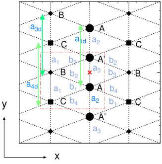
Figure 1: (Color online) Crystal structure of $\alpha$-(BEDT-TTF)₂I₃. There are four molecules A, A’, B, and C in a unit cell (dot-dashed line). The unit cell forms a square lattice, whereas each molecule is located on the triangular lattice. Transfer energies are given as $a_{1},\cdots,b_{4}$ for the nearest-neighbor (NN) sites and $a_{1d}$, $a_{3d}$, and $a_{4d}$ for the next-nearest-neighbor (NNN) sites. The cross denotes an inversion center between A and A’. $x$ ($y$) denotes a coordinate perpendicular to (along) a molecular stacking direction.

The TB model $H_{0}$ without spin degrees of freedom is expressed as

$$H_{0} = \sum_{i,j=1}^{N}\sum_{\alpha,\beta}t_{i,j;\alpha,\beta}a^{\dagger}_{i,\alpha}a_{j,\beta},$$ (3)

where $t_{i,j;\alpha,\beta}$ depicts the taransfer energy. $N$ is the total number of unit cells and $a^{\dagger}_{i,\alpha}$ denotes a creation operator of an electron on a molecule $\alpha$ in the $i$-th unit cell. Figure 1 shows a crystal structure of $\alpha$-(BEDT-TTF)₂I₃ used in the TB model. In the unit cell, there are four BEDT-TTF molecules $\alpha$ [= A(1), A’(2), B(3), and C(4)].

2.2 Transfer energies of TB model obtained by DFT

We derive the quantity $t_{i,j;\alpha,\beta}$ in Eq. (3) from first-principles DFT calculations. The explicit expression for the transfer energy is provided by

$$t_{\alpha,\beta}(\mathbf{R})=\langle\phi_{\alpha,0}|H_{k}|\phi_{\beta,\mathbf{R}}\rangle,$$ (4)

where $H_{k}$ is the one-body part of the ab initio Hamiltonian for $\alpha$-(BEDT-TTF)₂I₃. [9] $\phi_{\alpha,\mathbf{R}}$ denotes the maximally localized Wannier function (MLWF) spread over the BEDT-TTF molecule with $\alpha$ ($\beta$) representing distinct MLWFs and $\mathbf{R}$ indicating the location of the $j$-th unit cell relative to the $i$-th unit cell [32]. The crystal structure employed in our calculations is based on an experimental structure measured at 1.76 GPa [6], with structural optimization performed for hydrogen positions.

Equation (4) reveals that $t_{i,j;\alpha,\beta}$ relies not on the respective site but solely on the difference between the $i$-th and $j$-th sites. Subsequent to acquiring Bloch functions through the DFT calculations,[33, 34] the MLWFs were constructed utilizing the wannier90 code [35, 36]. Transfer energies were then computed on the basis of the overlaps between the four MLWFs. It is noteworthy that the center of each MLWF is positioned at the midpoint of the central C = C bonds in each BEDT-TTF molecule. The present DFT calculations are based on a pseudopotential technique and plane wave basis sets via the projected augmented plane wave method,[37] as implemented in the Vienna ab initio simulation package (VASP).[38, 39] The exchange-correlation functional used in this work is the generalized gradient approximation (GGA) proposed by Perdew, Burke, and Ernzerhof (PBE).[40] We set the cutoff energies to 400 and 645 eV for plane waves and augmentation charge, respectively. We employed a 4 x 4 x 2 uniform $\bm{k}$-point mesh with a Gaussian smearing method during self-consistent loops.

The obtained transfer energies $a_{1},\cdots,b_{4}$, $a_{1d},a_{3d}$, and $a_{4d}$ in Fig. 1 are listed in Table LABEL:table_1. The quantities $t_{\rm AA}$, $t_{\rm A^{\prime}A^{\prime}}$, $t_{\rm BB}$, and $t_{\rm CC}$ denote the diagonal elements corresponding to the on-site potential energy. Since the origin of energy is arbitrary, we take only the on-site potentials $V_{\rm B}$ and $V_{\rm C}$ measured from that of A and A’, which are defined by $V_{\rm B}\equiv t_{\rm BB}-t_{\rm AA}$ and $V_{\rm C}\equiv t_{\rm CC}-t_{\rm AA}$, with $t_{\rm AA}=t_{\rm A^{\prime}A^{\prime}}$ . The unit of energy is taken as eV.

Table 1: First-principles TB model parameters in eV, which are obtained from Eq. (4).

$t_{i,j;\alpha,\beta}(i\not=j)$
$a1$	$-0.0122$
$a2$	$-0.0239$
$a3$	0.0520
$b1$	0.1508
$b2$	0.1335
$b3$	0.0568
$b4$	0.0194
$a_{1d}$	0.0130
$a_{3d}$	0.0032
$a_{4d}$	0.0185

$t_{i,i;\alpha,\alpha}$
$t_{\rm AA}$	4.744677
$t_{\rm A^{\prime}A^{\prime}}$	4.744677
$t_{\rm BB}$	4.693977
$t_{\rm CC}$	4.678874

2.3 Electronic states

$H_{0}$ is diagonalized by $H_{0}|\gamma>=E_{\gamma}|\gamma>$, i.e.,

$$\sum_{\beta}h_{\alpha,\beta}(\bm{k})d_{\beta\gamma(\bm{k})} = E_{\gamma}(\bm{k})d_{\alpha\gamma}(\bm{k})\;,$$ (5)

where $h_{\alpha,\beta}(\bm{k})$ is the Fourier transform of Eq. (3) given in Appendix A. $E_{\gamma}(\bm{k})$ $(\gamma=1,\cdots,4)$ denotes the energy in the descending order. The Dirac point ($\bm{k}_{\rm D}$) is obtained from

$$E_{1}(\bm{k}_{\rm D})=E_{2}(\bm{k}_{\rm D})=\epsilon_{\rm D}\;,$$ (6)

where $E_{1}(\bm{k})$ denotes the conduction band and $E_{2}(\bm{k})$ denotes the valence band. The ZGS is found when $\epsilon_{\rm D}$ becomes equal to the chemical potential $\mu$. From the three-quarter-filled condition, $\mu$ is calculated by

$$\frac{1}{N}\sum_{\bm{k}}\sum_{\gamma}f(E_{\gamma}(\bm{k}))=3\;,$$ (7)

where $f(\epsilon)=1/(\exp[(\epsilon-\mu)/k_{\rm B}T]+1)$ with $T$ being temperature and the Boltzmann constant taken as $k_{\rm B}=1$.

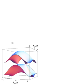
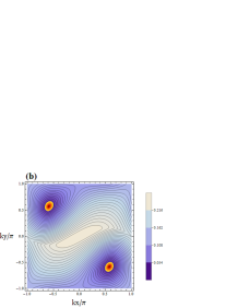
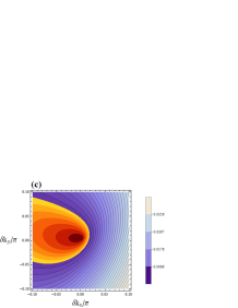
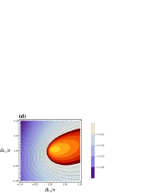
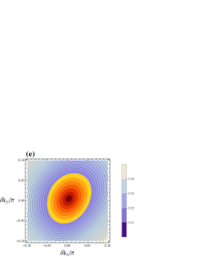
Figure 2: (Color online) (a) Conduction and valence bands given by $E_{1}(\bm{k})$ (upper band) and $E_{2}(\bm{k})$ (lower band). (b) Contour plots of $E_{1}(\bm{k})-E_{2}(\bm{k})$, where the yellow region including the Dirac point $\bm{k}_{\rm D}$ is given by $0<E_{1}(\bm{k})-E_{2}(\bm{k})<0.03$. (c) Contour plots of $E_{1}(\bm{k})$ around $\bm{k}_{\rm D}$, where $\delta\bm{k}=\bm{k}-\bm{k}_{\rm D}$. The yellow region corresponds to $0<E_{1}(\bm{k})-\epsilon_{\rm D}<0.005$. (d) Contour plots of $E_{2}(\bm{k})$ around $\bm{k}_{\rm D}$. The yellow region corresponds to $-0.005<E_{2}(\bm{k})-\epsilon_{\rm D}<0$. (e) Contour plots of $E_{1}(\bm{k})-E_{2}(\bm{k})$ around $\bm{k}_{\rm D}$. The yellow region corresponds to $0<E_{1}(\bm{k})-E_{2}(\bm{k})<0.02$.

Using the TB model with transfer energies given in Table LABEL:table_1, we examine the energy bands obtained from Eq. (5). The site potentials measured from that at A and A’ are given as $V_{B}=-0.0507$ and $V_{C}=-0.0650$. In the following, two bands of $E_{1}(\bm{k})$ and $E_{2}(\bm{k})$ are examined since $E_{3}(\bm{k})$ and $E_{4}(\bm{k})$ are located far below the chemical potential. The calculated energy bands are shown in Figs. 2(a)–2(e).

Figure 2(a) shows $E_{1}(\bm{k})$ (upper band) and $E_{2}(\bm{k})$ (lower band) for $\alpha$-(BEDT-TTF)₂I₃, which contact at the Dirac points $\pm\bm{k}_{\rm D}=\pm(-0.58,0.57)\pi$ with the energy $\epsilon_{\rm D}$ forming the ZGS. Figure 2(b) shows contour plots of $E_{1}(\bm{k})-E_{2}(\bm{k})$ providing $\pm\bm{k}_{\rm D}$.[41] Figures 2(c) and 2(d) show contour plots of the conduction band $E_{1}(\bm{k})$ and the valence band $E_{2}(\bm{k})$, respectively, with $\delta\bm{k}=\bm{k}-\bm{k}_{\rm D}$. Figure 2(e) shows magnified contour plots of $E_{1}(\bm{k})-E_{2}(\bm{k})$ around $\bm{k}_{\rm D}$. The ellipsoid of the contour suggests an anisotropy of the velocity of the Dirac cone with $v_{x}>v_{y}$.

Using $E_{\gamma}(\bm{k})$, we calculate DOS as

$$D(\omega)=\frac{1}{N}\sum_{\bm{k}}\sum_{\gamma}\delta(\omega-E_{\gamma}(\bm{k})),$$ (8)

which is shown in Fig. 3 as a function of $\omega-\mu_{0}$ with $\mu_{0}$ being $\mu$ at $T=0$. There is an asymmetry of DOS around $\omega=\mu_{0}$; DOS for the conduction band ($\omega>\mu_{0}$) is slightly larger than that for the valence band ($\omega<\mu_{0}$). The inset shows the $T$ dependence of the chemical potential $\mu$. Owing to the asymmetry of DOS, $\mu$ becomes smaller than $\mu_{0}$ at finite temperatures.

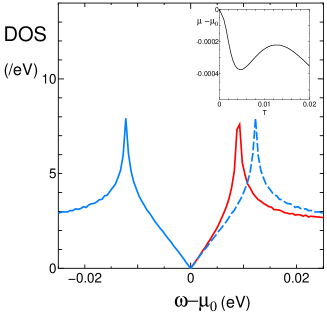
Figure 3: (Color online ) DOS as a function of $\omega-\mu_{0}$, where $\mu_{0}=\epsilon_{\rm D}=0.1679$ is $\mu$ at $T=0$. The blue dashed line denotes the symmetrized DOS using $D(\omega)$ with $\omega<\mu_{0}$. For the fixed $|\omega-\mu_{0}|(<0.01)$, DOS with $\omega>\mu_{0}$ (red solid line) is larger than that with $\omega<\mu_{0}$ (blue line). The inset denotes $\mu-\mu_{0}$ as a function of $T$.

3 Seebeck Effects

3.1 Seebeck coefficient

Using the linear response theory, [27, 28] the electric current density $\bm{j}=(j_{x},j_{y})$ is obtained from the electric field $\bm{E}=(E_{x},E_{y})$ and the temperature gradient $\nabla T$ as

$$j_{\nu}=L_{11}^{\nu}E_{\nu}-L_{12}^{\nu}\nabla_{\nu}T/T\;,\quad{\rm for}\ \nu=x,y\;,$$ (9)

where $L_{11}^{\nu}$ is the electrical conductivity $\sigma_{\nu}$[23] and $L_{12}^{\nu}$ is the thermoelectric conductivity in the $\nu$-direction. From Eq. (9), the Seebeck coefficient $S_{\nu}$ is given by

$$S_{\nu}(T) = \frac{L_{12}^{\nu}}{TL_{11}^{\nu}}\;.$$ (10)

We calculate $L_{11}^{\nu}$ and $L_{12}^{\nu}$ using the Sommerfeld–Bethe relation in the same way as we performed in the case of uniaxial pressure.[31] Details are shown in Appendix B.[29] The quantities $L_{11}^{\nu}$ and $L_{12}^{\nu}$ are calculated from the spectral conductivity $\sigma_{\nu}(\epsilon,T)$ defined by

$$\sigma_{\nu}(\epsilon,T) \equiv \frac{e^{2}}{\pi\hbar N}\sum_{\gamma,\gamma^{\prime}}\sum_{\bm{k}}v^{\nu}_{\gamma\gamma^{\prime}}(\bm{k})^{*}v^{\nu}_{\gamma^{\prime}\gamma}(\bm{k})$$

$$\times \frac{\Gamma_{\gamma}}{(\epsilon-E_{\gamma}(\bm{k}))^{2}+\Gamma_{\gamma}^{2}}\times\frac{\Gamma_{\gamma^{\prime}}}{(\epsilon-E_{\gamma^{\prime}}(\bm{k}))^{2}+\Gamma_{\gamma^{\prime}}^{2}}\;,$$

with $v^{\nu}_{\gamma\gamma^{\prime}}(\bm{k})=\sum_{\alpha\beta}$ $d_{\alpha\gamma}(\bm{k})^{*}(\partial h_{\alpha\beta}/\partial k_{\nu})d_{\beta\gamma^{\prime}}(\bm{k}).$ $\Gamma_{\gamma}$ denotes the damping of electrons in the $\gamma$ band. $h=2\pi\hbar$ and $e(>0)$ are Planck’s constant and the electric charge, respectively.

Since the spectral conductivity can be decomposed into intraband and interband contributions, the conductivity [23] and the Seebeck coefficient are also expressed as

$$\sigma_{\nu}(T) = \sum_{\gamma,\gamma^{\prime}}\sigma_{\nu}^{\gamma\gamma^{\prime}}(T)\;,$$ (12a)

$$S_{\nu}(T) = \sum_{\gamma,\gamma^{\prime}}S_{\nu}^{\gamma\gamma^{\prime}}(T)\;,$$ (12b)

with $(\gamma,\gamma^{\prime})$=(1,1), (1,2), (2,1), and (2,2), where $\gamma,\gamma^{\prime}=$ 1 and 2 correspond to the energy bands with $E_{1}(\bm{k})$ and $E_{2}(\bm{k})$, respectively ( See Appendix B).

To calculate the spectral conductivity, we need the $T$ dependence of $\Gamma_{\gamma}$. As in a previous paper,[31] we assume

$$\Gamma_{\gamma}=\Gamma+\Gamma_{\rm ph}^{\gamma}\;,$$ (13)

where $\Gamma$ comes from impurity scattering and $\Gamma_{\rm ph}^{\gamma}$ from phonon scattering:

$$\Gamma_{\rm ph}^{\gamma} = C_{0}R\times T|\xi_{\gamma,\bm{k}}|\;,$$ (14a)

$$R = \frac{\lambda}{\lambda_{0}}\;,$$ (14b)

where $\lambda=|g_{\bm{q}}|^{2}/\omega_{\bm{q}}$, $\xi_{\gamma,\bm{k}}=E_{\gamma}(\bm{k})-\mu$, $C_{0}=6.25\lambda_{0}/(2\pi v^{2})$, and $\lambda_{0}/2\pi v=0.1$. [22] $\lambda_{0}$ corresponds to $\lambda$ for an organic conductor[42, 43] and $\lambda$ becomes independent of $|\bm{q}|$ for a small $|\bm{q}|$. $R$ is taken as a parameter. We take $\Gamma=0.0005$ and $R=1$ in the present numerical calculation. [24, 31]

Figure 4(a) shows the $T$ dependence of $\sigma_{\nu}^{\gamma\gamma^{\prime}}$. We can see that the component of (2,2) coming from the valence band is larger than that of (1,1) from the conduction band, whereas the interband contribution (1,2) is much smaller. This is understood from the DOS of Dirac electrons, which is inversely proportional to the velocity of the Dirac cone. As shown in Fig. 3, the DOS of the valence band $(\omega<\mu_{0})$ is lower than that of the conduction band $(\omega>\mu_{0})$. Thus, the velocity of the valence band is higher than that of the conduction band, leading to $\sigma_{\nu}^{22}(T)>\sigma_{\nu}^{11}(T)$. Figure 4(b) shows the $T$ dependence of $S_{\nu}^{\gamma\gamma^{\prime}}$. It is natural that the component of (1,1) is negative since it comes from the conduction band (or electrons), whereas that of (2,2) is positive since it comes from the valence band (or holes). The interband contribution (1,2) is much smaller than the others. Thus, $S_{\nu}(T)\simeq S_{\nu}^{11}(T)+S_{\nu}^{22}(T)$ suggests a competition from contributions between the conduction and valence bands. Note that $S_{\nu}^{22}(T)>|S_{\nu}^{11}(T)|$, which is compatible with $\sigma_{\nu}^{22}(T)>\sigma_{\nu}^{11}(T)$.

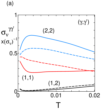
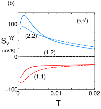
Figure 4: (Color online ) $T$ dependence of the components $(\gamma,\gamma^{\prime})$ of the (a) conductivity and (b) Seebeck coefficient. The solid and dashed lines correspond to $\nu=x$ and $\nu=y$, respectively.

Next, we examine the $T$ dependence of the Seebeck coefficients $S_{x}$ and $S_{y}$ as shown in Fig. 5. It is shown that both $S_{x}$ and $S_{y}$ are positive at finite temperatures and take a maximum at $T=0.002$ and $T=0.006$, respectively. The positive $S_{\nu}$ originates from $S_{\nu}^{22}(T)>|S_{\nu}^{11}(T)|$ as discussed above. This is also understood from the behavior of $\mu(T)$ in the inset of Fig. 3, which shows that $\mu(T)$ is lower than $\mu_{0}$, leading to the hole-like behavior at finite temperatures. Noting that the decrease in $\mu(T)-\mu_{0}\simeq-0.0002$ at $T=0.002$, it is suggested that a very small amount of electron doping gives rise to $S_{\nu}<0$.

Figure 5 also shows the corresponding conductivities, $\sigma_{x}$ and $\sigma_{y}$. Both $\sigma_{x}$ and $\sigma_{y}$ remain finite at $T=0$ owing to a quantum effect [44] and take a maximum around $T\simeq 0.003$. At lower temperatures, the increase in $\sigma_{\nu}$ originates from the Dirac cone, which gives a linear increase in DOS measured from the chemical potential. At higher temperatures, the decrease in $\sigma_{\nu}$ originates from the enhancement of the phonon scattering [Eq. (14a)]. The relation $\sigma_{x}>\sigma_{y}$ comes from the anisotropy of the Dirac cone,[44] which gives $v_{x}>v_{y}$, as shown in Fig. 2(e). There is a similarity of the $T$ dependence between $S_{\nu}$ and $\sigma_{\nu}$ since both quantities depend on the spectral conductivity. However, there is a difference in origin between $S_{\nu}$ and $\sigma_{\nu}$. $S_{\nu}$ is determined by the effects of competition between the valence and conduction bands, whereas $\sigma_{\nu}$ is obtained from the additive effects of the valence and conduction bands.

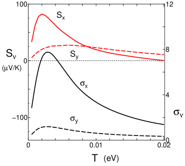
Figure 5: (Color online ) $T$ dependence of the Seebeck coefficients $S_{x}$ and $S_{y}$ (left axis) and the corresponding conductivities $\sigma_{x}$ and $\sigma_{y}$ (right axis). The unit of $\sigma_{\nu}$ is taken as $e^{2}/\hbar$. These quantities are calculated using $\mu(T)$ shown in the inset of Fig. 3.

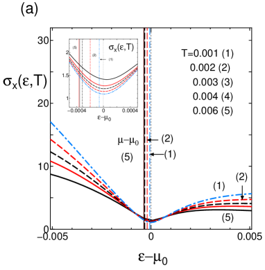
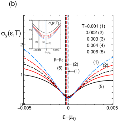
Figure 6: (Color online) $T$ dependence of the spectral conductivities $\sigma_{x}(\epsilon,T)$  (a) and $\sigma_{y}(\epsilon,T)$  (b) as a function of $\epsilon-\mu_{0}$ with fixed temperatures $T=$ 0.001 (1), 0.002 (2), 0.003 (3), 0.004 (4) and 0.006 (5). The vertical line shows $\mu-\mu_{0}$ for the corresponding temperatures. The inset denotes the respective $\sigma_{\nu}(\epsilon,T)$ with a magnified scale.

3.2 Spectral conductivity

Here, let us examine the sign of $S_{\nu}$ using the spectral conductivity $\sigma_{\nu}(\epsilon,T)$. When we expand $\sigma_{\nu}(\epsilon,T)$ as

$$\sigma_{\nu}(\epsilon,T) = \sigma_{\nu}(\mu,T)+\sigma^{\prime}_{\nu}(\mu,T)(\epsilon-\mu)$$ (15)

$$+\frac{1}{2}\sigma^{\prime\prime}_{\nu}(\mu,T)(\epsilon-\mu)^{2}+\cdots,$$

the thermoelectric conductivity $L_{12}^{\nu}(T)$ is given by [31]

$$eL_{12}^{\nu}(T) = -\frac{\pi^{2}}{3}\sigma^{\prime}_{\nu}(\mu,T)T^{2}-\frac{7\pi^{4}}{90}\sigma^{\prime\prime\prime}_{\nu}(\mu,T)T^{4}$$ (16)

$$+\cdots.$$

Note that the first term corresponds to the Mott formula when $T\rightarrow 0$, [45] and it indicates that $S_{\nu}(T)<0$ ($S_{\nu}(T)>0$) when $\sigma^{\prime}_{\nu}(\mu,T)>0$ ($\sigma^{\prime}_{\nu}(\mu,T)<0$).

Figures 6(a) and 6(b) show the spectral conductivities $\sigma_{x}(\epsilon,T)$  and $\sigma_{y}(\epsilon,T)$, resprctively as a function of $\epsilon-\mu_{0}$ at several temperatures. They show a common feature that the minimum of $\sigma_{\nu}(\epsilon,T)\;$($\nu=x$ and $y$) is found at $\epsilon-\mu_{0}\simeq 0$. The effect of temperature is seen for $|\epsilon-\mu_{0}|>0.001$. There is a small deviation of the minimum of $\sigma_{\nu}(\epsilon,T)\;$from $\mu_{0}$. It can be shown analytically that $\sigma_{\nu}(\epsilon,T)\;$takes the minimum at $\epsilon=\mu_{0}$ in the two-band model with the linear dispersion regardless of the tilting. Thus, the deviation of the minimum of $\sigma_{x}(\epsilon,T)$  from $\epsilon=\mu_{0}$ is ascribed to the energy band around the Dirac point, which deviates from the linear dispersion. The vertical lines denote $\epsilon=\mu(T)$ for the respective temperatures, which reads the tangent of $\sigma_{\nu}(\epsilon,T)\;$at $\epsilon=\mu(T)$. Since $\mu(T)<\mu_{0}$, $\sigma^{\prime}_{\nu}(\epsilon,T)<0$ at $\epsilon=\mu(T)$, suggesting $S_{\nu}(T)>0$ at any temperature. We can see that $\sigma_{x}(\epsilon,T)$  $>$ $\sigma_{y}(\epsilon,T)$, which is consistent with $v_{x}>v_{y}$ as discussed above. Furthermore, we find that the anisotropy of $\sigma_{x}(\epsilon,T)$  with respect to $\epsilon-\mu_{0}$ is larger than that of $\sigma_{y}(\epsilon,T)$. This can be understood from the energy bands shown in Figs. 2(c) and 2(d), where anisotropy along $\delta k_{x}$ is much larger than that along $\delta k_{y}$ owing to the tilting of the Dirac cone along the $k_{x}$ direction. Finally, the magnitude of $\sigma_{\nu}(\epsilon,T)\;$for $\epsilon-\mu_{0}<0$ is larger than $\sigma_{\nu}(\epsilon,T)\;$for $\epsilon-\mu_{0}>0$, which is consistent with the asymmetry of DOS as discussed in Fig. 4(a).

4 Summary and Discussion

We have examined the $T$ dependence of the Seebeck coefficient for the Dirac electrons in $\alpha$-(BEDT-TTF)₂I₃  under hydrostatic pressure using the improved TB model obtained from the first-principles DFT calculations with the experimentally determined crystal structure. To the best of our knowledge, the TB model presented in this paper is unique for explaining the Seebeck coefficient of the present organic conductor. Main results of this study are as follows: (i) The Seebeck coefficient is positive in both $x$- and $y$-directions, i.e., $S_{x}>0$ and $S_{y}>0$, indicating the hole-like behavior, which is consistent with $\mu(T)-\mu_{0}<0$. However, note that the sign of the Seebeck coefficient is determined not only from the sign of $\mu(T)-\mu_{0}$ but also from the difference between the energy dispersions of the conduction and valence bands. Although the quantitative understanding of such competition between the conduction and valence bands is complicated, it is demonstrated that an effective method of comprehending the sign of the Seebeck coefficient is to examine the energy derivative of the spectral conductivity, $\sigma_{\nu}(\epsilon,T)$, at $\epsilon=\mu(T)$. (ii) Another result obtained from the transfer energies of the present model is $\sigma_{x}>\sigma_{y}$ as seen from the behavior of the Dirac cone [Fig. 2(e)]. This is in sharp contrast to that of the model of the extended Hückel method, which shows $\sigma_{y}>\sigma_{x}$. [24] (iii) The analysis of the spectral conductivity suggests that $S_{\nu}<0$ can be realized by a small amount of electron doping, i.e., $\mu-\mu_{0}\simeq 0.0001$.

Let us compare our calculation result of $S_{\nu}$ with the experimental results of $\alpha$-(BEDT-TTF)₂I₃ under hydrostatic pressures. So far, two experiments have been reported. [26, 25] One is a measurement at $P$ = 1.5 GPa, [26] which shows that the positive $S_{\nu}$ has a small peak at around 50 K and then decreases as the temperature decreases up to 2 K. No sign change at low temperatures is predicted. This is consistent with our theoretical results of $S_{x}>0$ and $S_{y}>0$. Moreover, the existence of a maximum of $S_{\nu}$ is also consistent with our results. Another experiment is a measurement performed at $P$ = 1.9 GPa, where a sign change of $S_{x}$ occurs at around 3 K and the positive $S_{x}$ shows a peak at high temperatures. Such a sign change depends on the choice of samples, and we speculate that this sign change can be understood by assuming a small amount of electron doping, since the variation of the chemical potential is $\sim 0.0001$ for $T=0.001$ as discussed in this paper. Thus, the present TB model obtained from the DFT calculations explains successfully the Seebeck coefficient obtained from the experiments of $\alpha$-(BEDT-TTF)₂I₃, which depend on the doping amount. Finally, we comment on the anisotropy of the conductivities shown in Fig. 5, where $\sigma_{x}$ is much larger that $\sigma_{y}$. The experimental results show that $\sigma_{x}$ is about twice as much as $\sigma_{y}$ and their ratio is expected to increase for a clean sample.[46]

Appendix A Matrix elements in the TB model

The TB model $H_{0}$ in Eq. (3) is expressed as

$$H_{0} = \sum_{\bm{k}}\sum_{\alpha,\beta}h_{\alpha,\beta}(\bm{k})a^{\dagger}_{\alpha}(\bm{k})a_{\beta}(\bm{k})\;.$$ (17)

The Fourier transform for the operator $a_{j,\alpha}$ is defined as $a_{j,\alpha}=1/N^{1/2}\sum_{\bm{k}}a_{\alpha}(\bm{k})\exp[i\bm{k}\cdot\bm{r}_{j}]$, where $\bm{k}=(k_{x},k_{y})$ for the 2D case with $-\pi<k_{x},k_{y}\leq\pi$ and the lattice constant is taken as unity. Using a basis of four molecules in the unit cell ($\alpha$ = 1, 2, 3, and 4), we write the matrix element $h_{\alpha,\beta}(\bm{k})$ as

$$h_{12}(\bm{k}) = a_{3}+a_{2}Y\;,$$ (18a)

$$h_{13}(\bm{k}) = b_{3}+b_{2}X\;,$$ (18b)

$$h_{14}(\bm{k}) = b_{4}Y+b_{1}XY\;,$$ (18c)

$$h_{23}(\bm{k}) = b_{2}+b_{3}X\;,$$ (18d)

$$h_{24}(\bm{k}) = b_{1}+b_{4}X\;,$$ (18e)

$$h_{34}(\bm{k}) = a_{1}+a_{1}Y\;,$$ (18f)

$$h_{11}(\bm{k}) = t_{22}(\bm{k})=a_{1d}(Y+\bar{Y})\;,$$ (18g)

$$h_{33}(\bm{k}) = a_{3d}(Y+\bar{Y})+V_{\rm B}\;,$$ (18h)

$$h_{44}(\bm{k}) = a_{4d}(Y+\bar{Y})+V_{\rm C}\;,$$ (18i)

and $h_{\alpha,\beta}(\bm{k})=h_{\beta,\alpha}^{*}(\bm{k})$, where $X=\exp[ikx]=\bar{X}^{*}$ and $Y=\exp[iky]=\bar{Y}^{*}$. $k_{x}$ corresponds to the direction perpendicular to the molecular stacking axis.

Appendix B Spectral conductivity and Seebeck coefficient

The electrical and thermoelectric conductivities are respectively written as

$$L_{11}^{\nu} = \sigma_{\nu}(T)=\int_{-\infty}^{\infty}d\epsilon\left(-\frac{\partial f(\epsilon)}{\partial\epsilon}\right)\times\sigma_{\nu}(\epsilon,T)\;,$$

$$L_{12} = \frac{-1}{e}\int_{-\infty}^{\infty}d\epsilon\left(-\frac{\partial f(\epsilon)}{\partial\epsilon}\right)\times(\epsilon-\mu)\sigma_{\nu}(\epsilon,T)\;.$$

The spectral conductivity $\sigma_{\nu}(\epsilon,T)$ with $\nu=x$ and $y$ is calculated as [31]

$$\sigma_{\nu}(\epsilon,T) = \sum_{\gamma,\gamma^{\prime}}\sigma_{\nu}^{\gamma\gamma^{\prime}}(\epsilon,T)\;,$$ (21)

where

$$\sigma_{\nu}^{\gamma\gamma^{\prime}}(\epsilon,T) = \frac{e^{2}}{\pi\hbar N}\sum_{\bm{k}}v^{\nu}_{\gamma\gamma^{\prime}}(\bm{k})^{*}v^{\nu}_{\gamma^{\prime}\gamma}(\bm{k})$$

$$\times \frac{\Gamma_{\gamma}}{(\epsilon-E_{\gamma}(\bm{k}))^{2}+\Gamma_{\gamma}^{2}}\times\frac{\Gamma_{\gamma^{\prime}}}{(\epsilon-E_{\gamma^{\prime}}(\bm{k}))^{2}+\Gamma_{\gamma^{\prime}}^{2}}\;.$$

$v^{\nu}_{\gamma\gamma^{\prime}}(\bm{k})$ denotes a matrix element of the velocity given by $v^{\nu}_{\gamma\gamma^{\prime}}(\bm{k})=\sum_{\alpha\beta}$ $d_{\alpha\gamma}(\bm{k})^{*}(\partial h_{\alpha\beta}/\partial k_{\nu})d_{\beta\gamma^{\prime}}(\bm{k}).$ Using $\sigma_{\nu}^{\gamma\gamma^{\prime}}(\epsilon,T)$, we obtain the Seebeck coefficient $S_{\nu}$ by

$$S_{\nu}(T)=\frac{L_{12}^{\nu}}{TL_{11}^{\nu}}=\sum_{\gamma,\gamma^{\prime}}S_{\nu}^{\gamma\gamma^{\prime}}(T)$$ (23)

where

$$S_{\nu}^{\gamma\gamma^{\prime}}(T) = \frac{1}{TL_{11}^{\nu}}\times$$

$$\frac{-1}{e}\int_{-\infty}^{\infty}d\epsilon\left(-\frac{\partial f(\epsilon)}{\partial\epsilon}\right)\times(\epsilon-\mu)\sigma_{\nu}^{\gamma\gamma^{\prime}}(\epsilon,T)\;,$$

References

- [1] K. Kajita, Y. Nishio, N. Tajima, Y. Suzumura, and A. Kobayashi, J. Phys. Soc. Jpn. 83, 072002 (2014).
- [2] T. Mori, A. Kobayashi, Y. Sasaki, H. Kobayashi, G. Saito, and H. Inokuchi, Chem. Lett. 13, 957 (1984).
- [3] S. Katayama, A. Kobayashi, and Y. Suzumura, J. Phys. Soc. Jpn. 75, 054705 (2006).
- [4] A. Kobayashi, S. Katayama, K. Noguchi, and Y. Suzumura, J. Phys. Soc. Jpn. 73, 3135 (2004).
- [5] R. Kondo, S. Kagoshima, and J. Harada, Rev. Sci. Instrum. 76, 093902 (2005).
- [6] R. Kondo, S. Kagoshima, N. Tajima, and R. Kato, J. Phys. Soc. Jpn. 78, 114714 (2009).
- [7] A. Kobayashi, S. Katayama, Y. Suzumura, and H. Fukuyama, J. Phys. Soc. Jpn. 76, 034711 (2007).
- [8] M. O. Goerbig, J.-N. Fuchs, G. Montambaux, and F. Pichon, Phys. Rev. B 78, 045415 (2008).
- [9] H. Kino and T. Miyazaki, J. Phys. Soc. Jpn. 75, 034704 (2006).
- [10] P. Alemany, J.-P. Pouget, and E. Canadel, Phys. Rev. B 85 195118 (2012).
- [11] Y. Takano, K. Hiraki, Y. Takada, H. M. Yamamoto, and T. Takahashi, J. Phys. Soc. Jpn. 79, 104704 (2010).
- [12] M. Hirata, K. Ishikawa, K. Miyagawa, M. Tamura, C. Berthier, D. Basko, A. Kobayashi, G. Matsuno, and K. Kanoda, Nat. Commun. 7, 12666 (2016).
- [13] N. Tajima, R.. Kato, S. Sugawara, Y. Nishio, and K. Kajita, Phys. Rev. B 85, 033401 (2012).
- [14] S. Katayama, A. Kobayashi, and Y. Suzumura, Eur. Phys. J. B 67, 139 (2009).
- [15] A. Kobayashi, Y. Suzumura, and H. Fukuyama, J. Phys. Soc. Jpn. 77, 064718 (2008).
- [16] K. Kajita, T. Ojiro, H. Fujii, Y. Nishio, H. Kobayashi, A. Kobayashi, and R. Kato, J. Phys. Soc. Jpn. 61, 23 (1992).
- [17] N. Tajima, M. Tamura, Y. Nishio, K. Kajita, and Y. Iye, J. Phys. Soc. Jpn. 69, 543 (2000).
- [18] N. Tajima, A. Ebina-Tajima, M. Tamura, Y. Nishio, and K. Kajita, J. Phys. Soc. Jpn. 71, 1832 (2002).
- [19] N. Tajima, S. Sugawara, M. Tamura, R. Kato, Y. Nishio, and K. Kajita, EPL 80, 47002 (2007).
- [20] D. Liu, K. Ishikawa, R. Takehara, K. Miyagawa, M. Tanuma, and K. Kanoda, Phys. Rev. Lett. 116, 226401 (2016).
- [21] N. M. R. Peres, F. Guinea, and A. H. Castro Neto, Phys. Rev. B 83,125411 (2006).
- [22] Y. Suzumura and M. Ogata, Phys. Rev. B 98, 161205 (2018).
- [23] S. Katayama, A. Kobayashi, and Y. Suzumura, J. Phys. Soc. Jpn. 75, 023708 (2006).
- [24] Y. Suzumura and M. Ogata, J. Phys. Soc. Jpn. 90, 044709 (2021).
- [25] R. Kitamura, N. Tajima, K. Kajita, R. Reizo, M. Tamura, T. Naito, and Y. Nishio, JPS Conf. Proc. 1, 012097 (2014); N. Tajima, private communication.
- [26] T. Konoike, M. Sato, K. Uchida, and T. Osada, J. Phys. Soc. Jpn. 82, 073601 (2013).
- [27] R. Kubo, J. Phys. Soc. Jpn. 12, 570 (1957).
- [28] J. M. Luttinger, Phys. Rev. 135, A1505 (1964)
- [29] M. Ogata and H. Fukuyama, J. Phys. Soc. Jpn. 88, 074703 (2019).
- [30] D. Ohki, Y. Omori, and A. Kobayashi. Phys. Rev. B 101, 245201 (2020): They examined the Sebeck coefficient along the -direction using the transfer energies obtained by DFT [9] and employing an interpolation between low and and high temperatures, where the former case corresponds to Ref. \citenKatayama_EPJ. In this case, is slightly larger than . [24]
- [31] Y. Suzumura and M. Ogata, Phys. Rev. B 107, 195416 (2023).
- [32] T. Tsumuraya and Y. Suzumura, Eur. Phys. J.B, 94, 17 (2021).
- [33] P. Hohenberg and W. Kohn, Phys. Rev. 136, B864 (1964).
- [34] W. Kohn and L. J. Sham, Phys. Rev. 140, A1133 (1965).
- [35] N. Marzari and D. Vanderbilt, Phys. Rev. B 56, 12847 (1997).
- [36] I. Souza, N. Marzari, and D. Vanderbilt, Phys. Rev. B 65, 035109 (2001).
- [37] P. E. Blöchl, Phys. Rev. B 50, 17953 (1994).
- [38] G. Kresse and J. Furthmüller, Phys. Rev. B 54 11169 (1996).
- [39] G. Kresse and D. Joubert, Phys. Rev. B 59, 1758 (1999).
- [40] J. P. Perdew, K. Burke, and M. Ernzerhof, Phys. Rev. Lett. 77, 3865 (1996).
- [41] F. Piéchon, Y. Suzumura, and T. Morinari, J. Phys: Conf. Series 603, 012010 (2015). The location of a pair of Dirac points depends on the choice of the sign of transfer energies, where another choice corresponds to repaced by .
- [42] M. J. Rice, L. Pietronero, and P. Brüesh, Solid State Commun. 21, 757 (1977).
- [43] H. Gutfreund, C. Hartzstein, and M. Weger, Solid State Commun. 36, 647 (1980).
- [44] Y. Suzumura, I. Proskurin, and M. Ogata, J. Phys. Soc. Jpn. 83, 023701 (2014).
- [45] M. Jonson and G.D. Mahan, Phys. Rev. B 21, 4223 (1980).
- [46] N. Tajima, private communication.