Planet Formation by Gas-Assisted Accretion of Small Solids

Abstract

We compute the accretion efficiency of small solids, with radii $1\,\mathrm{cm}\leq R_{s}\leq 10\,\mathrm{m}$, on planets embedded in gaseous disks. Planets have masses $3\leq\mbox{$M_{p}$}\leq 20$ Earth masses ($M_{\oplus}$) and orbit within $10\,\mbox{au}$ of a solar-mass star. Disk thermodynamics is modeled via three-dimensional radiation-hydrodynamic calculations that typically resolve the planetary envelopes. Both icy and rocky solids are considered, explicitly modeling their thermodynamic evolution. Maximum efficiencies of $1\leq R_{s}\leq 100\,\mathrm{cm}$ particles are generally $\lesssim 10$%, whereas $10\,\mathrm{m}$ solids tend to accrete efficiently or be segregated beyond the planet’s orbit. A simplified approach is applied to compute the accretion efficiency of small cores, with masses $\mbox{$M_{p}$}\leq 1\,\mbox{$M_{\oplus}$}$ and without envelopes, for which efficiencies are approximately proportional to $M_{p}^{2/3}$. The mass flux of solids, estimated from unperturbed drag-induced drift velocities, provides typical accretion rates $d\mbox{$M_{p}$}/dt\lesssim 10^{-5}\,\mathrm{\mbox{$M_{\oplus}$}\,yr^{-1}}$. In representative disk models with an initial gas-to-dust mass ratio of $70$–$100$ and total mass of $0.05$–$0.06\,\mbox{$M_{\odot}$}$, solids’ accretion falls below $10^{-6}\,\mathrm{\mbox{$M_{\oplus}$}\,yr^{-1}}$ after $1$–$1.5\,\mbox{Myr}$. The derived accretion rates, as functions of time and planet mass, are applied to formation calculations that compute dust opacity self-consistently with the delivery of solids to the envelope. Assuming dust-to-solid coagulation times of $\approx 0.3\,\mbox{Myr}$ and disk lifetimes of $\approx 3.5\,\mbox{Myr}$, heavy-element inventories in the range $3$–$7\,\mbox{$M_{\oplus}$}$ require that $\approx 90$–$150\,\mbox{$M_{\oplus}$}$ of solids cross the planet’s orbit. The formation calculations encompass a variety of outcomes, from planets a few times $M_{\oplus}$, predominantly composed of heavy elements, to giant planets. Peak luminosities during the epoch of solids’ accretion range from $\approx 10^{-7}$ to $\approx 10^{-6}\,L_{\odot}$.

—

1 Introduction

Classic theories of planet formation assume that initial growth proceeds by collisions with planetesimals, bodies ranging in size from a fraction to hundreds of kilometers (e.g., Lissauer, 1993). Relict populations of these bodies are found in the asteroid and Kuiper belts (e.g., Bourdelle de Micas et al., 2022; Morbidelli & Nesvorný, 2020). The path to formation of planetesimals around stars remains mysterious, but conventional wisdom generally assumes that they are assembled from aggregates of much smaller particles, which are collected through some hydrodynamical process (in the circumstellar gas) and eventually clump together under their own gravity (see, e.g., Weiss et al., 2023, and references therein). These smaller particles, whose presence can be inferred from observations of protoplanetary disks (e.g., Natta et al., 2007; Andrews, 2020), would form through coagulation of primordial dust grains entrained in the gas.

This scenario for planetesimal formation has led to the suggestion that swarms of “small particles” orbiting a star in a protoplanetary disk may directly supply solid material to emerging planetary embryos and planets, determining their heavy-element inventories (Ormel & Klahr, 2010; Lambrechts & Johansen, 2012). Over the past decade, such delivery mode of solids has been referred to as “pebble accretion”. However, despite the terminology, these solids are unrelated to clastic rocks and are not required to fulfill the geological definition (Gary et al., 1972). In fact, they are not characterized by size or composition but rather by drag interaction with circumstellar gas, corresponding to Stokes numbers (see below) in the range between $\sim 10^{-3}$ and $\approx 1$ (Drazkowska et al., 2023). These numbers quantify the coupling timescale, in units of the orbital time (i.e., the inverse of the Keplerian frequency), between particle and gas dynamics. The Stokes number is proportional to the radius and material density of a particle, and inversely proportional to the gas density. Therefore, according to current terminology, astrophysical pebbles orbiting in a solar-nebula type of disk, between $\approx 1$ and $\approx 10\,\mbox{au}$, can range from sub-mm silicate grains (i.e., astrophysical dust, D’Alessio et al., 2001) to meter-size ice blocks. At larger distances, as gas density lowers, smaller particles would be considered as astrophysical pebbles (and the opposite would occur closer to the star). An overview of typical outcomes from pebble accretion calculations can be found in, e.g., Johansen & Lambrechts (2017), Drazkowska et al. (2023) and references therein.

Herein, we build first-principle numerical models of gas and solids thermodynamics. Since Stokes numbers cannot be constrained in the calculations (because they depend on primitive variables), we consider specific particle sizes (from $1\,\mathrm{cm}$ to $10\,\mathrm{m}$) and compositions (SiO₂ and H₂O), and will refer to these particles simply as “small solids”. Overlap with the domain of astrophysical pebbles varies according to local gas conditions.

The largest difference between planetesimals and small-solids accretion scenarios rests on their dynamics as they evolve in circumstellar gas. On the one hand, drag forces only provide a correction to the Keplerian orbits of the large bodies (Whipple, 1973). The drag-induced drifting timescale of $1\,\mathrm{km}$ planetesimals is $\sim 10^{6}$ orbital periods (in the $1$–$10\,\mbox{au}$ region), hence radial mobility due to aerodynamic drag can be largely ignored during planet formation. The accretion rate on a planet is determined by the local surface density of solids and by a characteristic cross-section for collisions, which can be enhanced by gravitational focusing and atmospheric drag (see, e.g., Pollack et al., 1996; Inaba & Ikoma, 2003). On the other hand, drag forces strongly affect the motion of small solids (Weidenschilling, 1977). Radial drift occurs on much shorter timescales than those of planetesimals. Hence, accretion is a non-local process. Global transport of solids through the disk determines the availability of supply and gas thermodynamics at and below the orbital length-scale determines the probability of accretion. The former cannot be evaluated without a global model of the circumstellar gas. The latter requires modeling tidal interactions between the planet and the disk (e.g., Morbidelli & Nesvorny, 2012) and gas dynamics in proximity of the planet (e.g., Picogna et al., 2018; Popovas et al., 2018). Therefore, any outcome of a planet formation calculation based on small-solids accretion is bound to depend on both local and remote gas thermodynamics. The applicability of generic formulations of accretion rates, found in the literature, is obviously limited by underlying assumptions (see, e.g., Lambrechts & Johansen, 2012; Drazkowska et al., 2023).

Planetesimal accretion proceeds as long as there is material in a region, the “feeding zone”, spanning a few Hill radii on either side of the planet’s orbit. Once this zone is depleted, accretion is much reduced and limited to the resupply rate into the region (e.g., Pollack et al., 1996; D’Angelo et al., 2014). Small-solids accretion can proceed as long as there is transport of material across the planet’s orbit, which can be hindered by overall depletion of solids, dissipating gas, and disk-planet tidal interactions.

In terms of interior compositions, the heavy-element inventory provided by the two accretion scenarios may differ since solids are accreted locally in one case and (effectively) remotely in the other. However, if planetesimals form out of small solids, which have drifted considerable distances prior to clumping together, planetesimals too can have (largely or to some extent) non-local compositions. Hence, diversity in compositions may not discriminate between the two scenarios. Differences in heavy-element stratification may also be difficult to ascertain. Clearly, small and large solids may coexist (e.g., Kessler & Alibert, 2023), although mass partitioning would depend on the mechanism that converts one population into the other (see, e.g., Drazkowska et al., 2023; Weiss et al., 2023, and references therein).

Herein, we present direct calculations of small-solids accretion, based on three-dimensional radiation-hydrodynamics calculations of disks with embedded planets that resolve the planetary envelope. Models also account for the thermal evolution of the particles. We focus on planet masses between $3$ and $20\,\mbox{$M_{\oplus}$}$. These calculations provide the accretion efficiency (or probability) of the particles on the planets at different orbital locations ($1$ to $10\,\mbox{au}$) and disk conditions. The accretion efficiency is the fraction of the local accretion rate of solids intercepted by the planet. The results are complemented with those obtained from a simpler approach, adopted to compute the accretion efficiency of bare cores (i.e., without a gaseous envelope) less massive than one Earth mass. The global transport of small solids, computed from drag-induced drift velocities in unperturbed disks, is combined with the accretion efficiencies to provide the accretion rates of the planets. These rates are then applied to actual formation and structure calculations, which compute dust opacity in the planet’s envelope self-consistently with the delivery of solids. These latter calculations are intended as demonstration of the framework provided herein and do not target any specific planet.

In the following, the orbital dynamics of small solids in unperturbed and perturbed disks is described in Section 2. The radiation-hydrodynamics models and accretion efficiencies of envelope-bearing planets are presented in Section 3; the accretion efficiencies of small, bare-core planets are discusses in Section 4. The formation calculations are presented in Section 5. Finally, our conclusions are summarized in Section 6.

2 Drag-Induced Orbital Decay of Solids

2.1 Dynamics in Unperturbed Disks

Small solids orbiting a star in a smooth unperturbed disk may experience strong drag forces exerted by the gas, and thus undergo rapid orbital decay. Assuming that the solids’ mass is locally much smaller than the gas mass, the time required for the velocity of a solid particle, $\boldsymbol{u}_{s}$, to converge toward the gas velocity, $\boldsymbol{u}_{g}$, is

$$\tau_{s}=\frac{|\boldsymbol{u}_{g}-\boldsymbol{u}_{s}|}{|\boldsymbol{a}_{D}|},$$ (1)

where $\boldsymbol{a}_{D}$ is the drag acceleration. The time $\tau_{s}$ is referred to as the “stopping time” of the particle (Whipple, 1973; Weidenschilling, 1977). Indicating with $\rho_{g}$ and $\rho_{s}$ respectively the gas and solid density, $R_{s}$ the particle radius, and $a_{s}$ its orbital distance, Equation (1) becomes (Whipple, 1973; Weidenschilling, 1977)

$$\tau_{s}=\frac{8}{3}\left(\frac{1}{C_{D}}\right)\left(\frac{\rho_{s}}{\rho_{g}}\right)\left(\frac{R_{s}}{|\boldsymbol{u}_{g}-\boldsymbol{u}_{s}|}\right).$$ (2)

The drag coefficient, $C_{D}$, is a function of the thermodynamic properties of both gas and solids. In the free-molecular flow regime (i.e., for very small particles), $C_{D}|\boldsymbol{u}_{g}-\boldsymbol{u}_{s}|$ tends to a constant, hence $\tau_{s}\propto R_{s}$.

The rotation rate of the gas, $\Omega_{g}$, is generally different from the Keplerian rate, $\Omega_{\mathrm{K}}$, and depends on the radial gradient of the gas pressure, $P_{g}$, typically a function of gas density and temperature, $T_{g}$. By requiring conservation of the gas linear momentum in the disk’s radial direction $r$, it can be approximated as

$$\Omega_{g}^{2}\approx\frac{1}{r}\left(\frac{\partial\Phi}{\partial r}\right)+\frac{1}{r\rho_{g}}\left(\frac{\partial P_{g}}{\partial r}\right),$$ (3)

$\Phi$ being the gravitational potential in the disk. Neglecting gas self-gravity, $\partial\Phi/\partial r=r\Omega^{2}_{\mathrm{K}}$ and Equation (3) applied to the mid-plane reduces to

$$\Omega_{g}\approx\Omega_{\mathrm{K}}\sqrt{1-\eta\left(\frac{H_{g}}{a_{s}}\right)^{2}},$$ (4)

where $H_{g}$ is the disk’s pressure scale-height at the mid-plane. The quantity $\eta$ depends on the normalized gradients $\partial\ln{\rho_{g}/\partial\ln{r}}$ and $\partial\ln{T_{g}/\partial\ln{r}}$ (see, e.g., Takeuchi & Lin, 2002; Tanaka et al., 2002), and is of order unity. Hereafter, $\eta$ is included in the ratio $H_{g}/a_{s}$. For typical protoplanetary disks, $(\Omega_{\mathrm{K}}-\Omega_{g})/\Omega_{\mathrm{K}}\approx(H_{g}/a_{s})^{2}/2$ is on the order of a percent or less (e.g., D’Alessio et al., 1998).

The mid-plane (non-transient) velocity of a particle subject to drag can be approximated to (e.g., Chiang & Youdin, 2010, and references therein)

$$\dot{a}_{s} \approx -\frac{a_{s}\Omega^{2}_{\mathrm{K}}(H_{g}/a_{s})^{2}\tau_{s}}{1+(\tau_{s}\Omega_{\mathrm{K}})^{2}}$$ (5)

$$\dot{\phi}_{s} \approx \Omega_{\mathrm{K}}-\left(\frac{1}{2}\right)\frac{\Omega_{\mathrm{K}}(H_{g}/a_{s})^{2}}{1+(\tau_{s}\Omega_{\mathrm{K}})^{2}},$$ (6)

$\phi_{s}$ being the azimuth angle of the particle. Equations (5) and (6) assume a negligible radial component of $\boldsymbol{u}_{g}$. Quantity $\tau_{s}\Omega_{\mathrm{K}}$ is referred to as the Stokes number of the particle. For $\tau_{s}\Omega_{\mathrm{K}}\gg 1$, the orbital decay timescale is $\tau_{D}=a_{s}/|\dot{a}_{s}|\approx(a_{s}/H_{g})^{2}\tau_{s}$ ($\gg\tau_{s}$). For $\tau_{s}\Omega_{\mathrm{K}}=1$, the decay timescale attains its minimum, $\tau_{D}\approx 2(a_{s}/H_{g})^{2}/\Omega_{\mathrm{K}}$. For $\tau_{s}\Omega_{\mathrm{K}}\ll 1$, the limit of a fully-coupled solid, $|\dot{a}_{s}|/a_{s}\approx\Omega^{2}_{\mathrm{K}}(H_{g}/a_{s})^{2}\tau_{s}$ and the radial displacement converges to that of the gas.

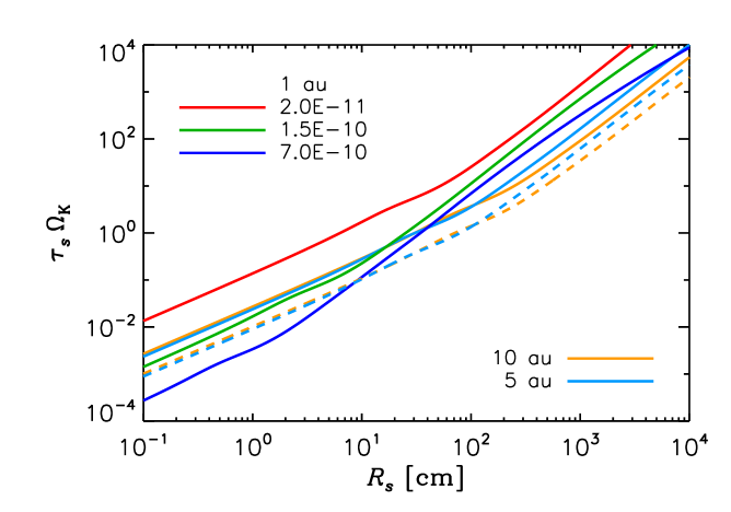
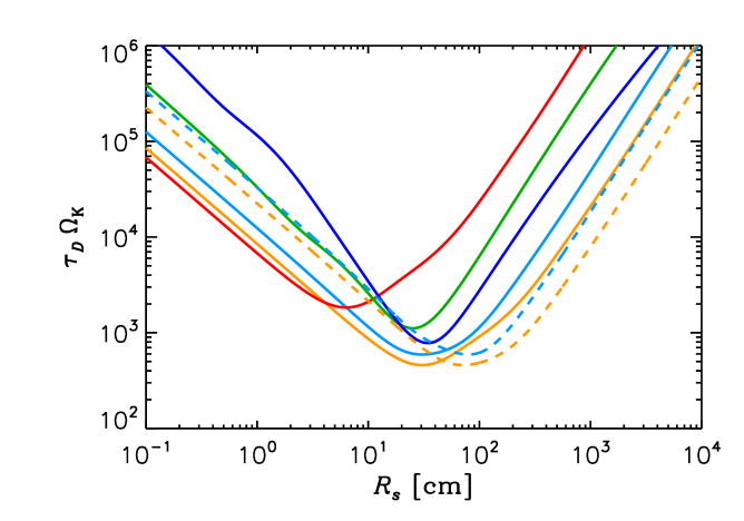
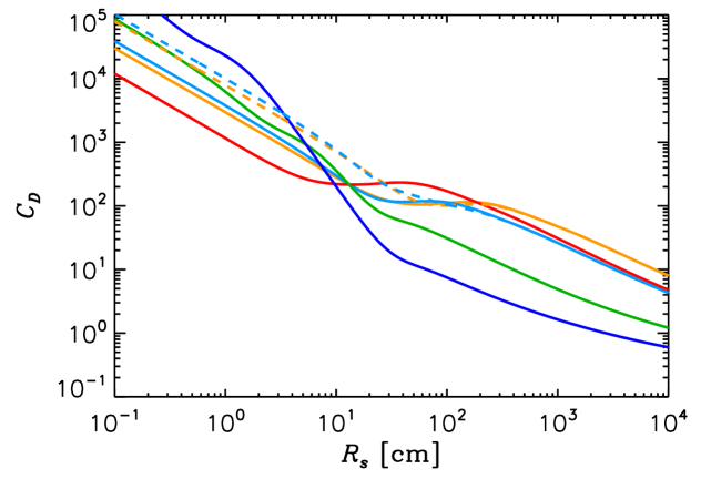
Figure 1: Stopping time $\tau_{s}$ (top) and orbital decay time $\tau_{D}$ (middle) of rocky (solid lines) and icy (dashed lines) particles of radius $R_{s}$, orbiting in a smooth and unperturbed protoplanetary disk. Time $\tau_{s}$ is computed by inverting Equation (2) and $\tau_{D}=a_{s}/|\dot{a}_{s}|$ (see Equation (5)). The drag coefficient $C_{D}$ (DP15) is also shown (bottom). Different lines refer to different disk locations and/or gas densities (as indicated in $\mathrm{g\,cm}^{-3}$) and temperatures (see also Table 1).

Using the coefficient $C_{D}$ reported in D’Angelo & Podolak (2015, hereafter DP15), which depends on $|\boldsymbol{u}_{g}-\boldsymbol{u}_{s}|$ and hence on $\tau_{s}$, Equation (2) can be inverted to provide a function $\tau_{s}=\tau_{s}(R_{s})$, plotted in Figure 1 (top panel). Through Equation (5), one can then recover the timescale for drag-induced orbital decay, $\tau_{D}$ (middle panel). For reference, $C_{D}$ is plotted in the bottom panel. The results in Figure 1 are based on disk thermodynamic conditions relevant to the radiation-hydrodynamics calculations described in Section 3, also detailed in Table 1. Under such conditions, $\tau_{s}\Omega_{\mathrm{K}}\approx 1$ when $R_{s}$ is a few times $10$ to $\approx 100\,\mathrm{cm}$. Smaller particles may satisfy the condition $\tau_{s}\Omega_{\mathrm{K}}\approx 1$ in a low density disk. The timescale $\tau_{D}$ has a minimum of a few hundred orbital periods, or less, and diverges as $R_{s}\rightarrow 0$ ($\tau_{s}\Omega_{\mathrm{K}}\rightarrow 0$) because the drift velocity $|\dot{a}_{s}|\propto\Omega^{2}_{\mathrm{K}}\tau_{s}a_{s}$ approaches zero. In this limit, however, $\dot{a}_{s}$ converges to the radial velocity of the gas, $u^{r}_{g}$, which cannot be neglected. In such cases, a corrected version of Equation (5) is (see, e.g., Takeuchi & Lin, 2002)

$$\dot{a}_{s}\approx\frac{u^{r}_{g}-a_{s}\Omega^{2}_{\mathrm{K}}(H_{g}/a_{s})^{2}\tau_{s}}{1+(\tau_{s}\Omega_{\mathrm{K}})^{2}}.$$ (7)

In the classic theory of accretion disks (e.g., Lynden-Bell & Pringle, 1974; Pringle, 1981),

$$u^{r}_{g}=-\frac{3}{2}\frac{\nu_{g}}{r}\left[1+2\frac{\partial\ln{(\nu_{g}\Sigma_{g})}}{\partial\ln{r}}\right],$$ (8)

in which $\nu_{g}$ and $\Sigma_{g}$ are respectively the kinematic viscosity and surface density of the gas. Writing the kinematic viscosity as $\nu_{g}=\alpha_{g}H^{2}_{g}\Omega_{\mathrm{K}}$ (Shakura & Sunyaev, 1973), if $\partial\ln{(\nu_{g}\Sigma_{g})}/{\partial\ln{r}}\ll 1$ then the bracket in Equation (8) is $\approx 1$, and the correction term in Equation (7) is negligible as long as $\tau_{s}\Omega_{\mathrm{K}}\gg\alpha_{g}$.

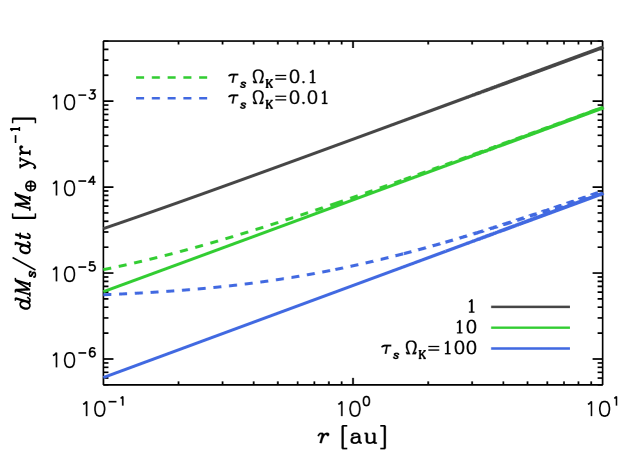
Figure 2: Accretion rate of solids through a disk according to Equation (9), with $u^{r}_{g}\approx-(3/2)\nu_{g}/r$ (see text), for particles of different stopping times, $\tau_{s}$, as indicated. The disk’s gas scale-height is $H_{g}\propto r^{9/7}$ (Chiang & Youdin, 2010). A reference surface density of solids of $\Sigma_{s}=1\,\mbox{$\mathrm{g\,cm}^{-2}$}$ is applied throughout ($dM_{s}/dt\propto\Sigma_{s}$).

Indicating with $\Sigma_{s}$ the solids’ surface density, the mass accretion rate of solids through an unperturbed disk is $dM_{s}/dt=-2\pi\Sigma_{s}a_{s}\dot{a}_{s}$. Applying Equation (7), the accretion rate becomes

$$\frac{dM_{s}}{dt}\approx 2\pi\!\left[\frac{(H_{g}/a_{s})^{2}\Omega_{\mathrm{K}}\tau_{s}-u^{r}_{g}/(a_{s}\Omega_{\mathrm{K}})}{1+(\tau_{s}\Omega_{\mathrm{K}})^{2}}\right]\!a^{2}_{s}\Sigma_{s}\Omega_{\mathrm{K}}.$$ (9)

Neglecting the term in $u^{r}_{g}$, maximum accretion occurs for $\tau_{s}\Omega_{\mathrm{K}}\approx 1$, when $dM_{s}/dt\approx\pi a^{2}_{s}\Sigma_{s}\Omega_{\mathrm{K}}(H_{g}/a_{s})^{2}$. At this rate, a mass of solids equal to $\pi a^{2}_{s}\Sigma_{s}$ would be transported through the radius $r=a_{s}$ in a timescale $(a_{s}/H_{g})^{2}/\Omega_{\mathrm{K}}$, or $\sim 10^{3}$ years at $r=10\,\mbox{au}$. In the de-coupled regime, $\tau_{s}\Omega_{\mathrm{K}}\gg 1$, $dM_{s}/dt\approx 2\pi a^{2}_{s}\Sigma_{s}\Omega_{\mathrm{K}}(H_{g}/a_{s})^{2}/(\tau_{s}\Omega_{\mathrm{K}})$ whereas in the opposite limit, $\tau_{s}\Omega_{\mathrm{K}}\ll 1$, $dM_{s}/dt\approx 2\pi a^{2}_{s}\Sigma_{s}\Omega_{\mathrm{K}}(H_{g}/a_{s})^{2}\tau_{s}\Omega_{\mathrm{K}}$. In the well-coupled regime, if $\tau_{s}\Omega_{\mathrm{K}}\lesssim\alpha_{g}$, the term in $u^{r}_{g}$ cannot be neglected and Equation (9) implies possible stalling or outward transport of solids in expanding disk regions (where $u^{r}_{g}>0$, Lynden-Bell & Pringle, 1974) or in transition regions (see Equation (8)).

Equation (9) is plotted in Figure 2, for a radially constant value of $\Sigma_{s}=1\,\mbox{$\mathrm{g\,cm}^{-2}$}$ and $u^{r}_{g}\approx-(3/2)\nu_{g}/r$, in which $\nu_{g}$ is constant and corresponds to $\alpha_{g}\approx 0.005$ at $1\,\mbox{au}$ ($H_{g}\propto r^{9/7}$). The effect of $u^{r}_{g}$ can be seen when $\tau_{s}\Omega_{\mathrm{K}}\lesssim\alpha_{g}$ ($\alpha_{g}$ is roughly proportional to $1/r$). The curves in the figure should only be interpreted as the value at $r$ for the imposed $\Sigma_{s}$. In fact, if $\partial\dot{M}_{s}/\partial r\neq 0$, mass conservation requires that

$$\frac{\partial\Sigma_{s}}{\partial t}=\frac{1}{2\pi r}\frac{\partial\dot{M}_{s}}{\partial r}+\Lambda(t,r),$$ (10)

where $\Lambda$ includes source/sink terms to account for, e.g., ongoing coagulation of solids from dust.

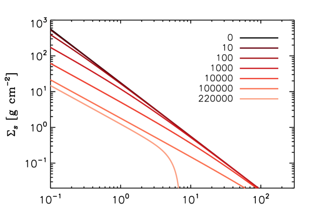
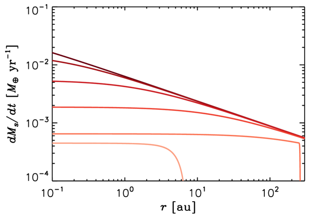
Figure 3: Top: Solution of Equation (10) by imposing $\tau_{s}\Omega_{\mathrm{K}}=1$ in Equation (9) and the initial gaseous nebula model of Chiang & Youdin (2010) (see text for details). Times in the legend are in years. The disk’s gas scale-height $H_{g}$ is constant in time. Bottom: Accretion rate of solids corresponding to the evolution of $\Sigma_{s}$ in the top panel.

A solution of Equation (10) is plotted in Figure 3, requiring that $\tau_{s}\Omega_{\mathrm{K}}=1$ in Equation (9). The initial conditions are based on the nebula model of Chiang & Youdin (2010), with a total gas mass of $0.055\,\mbox{$M_{\odot}$}$ ($\Sigma_{g}\propto r^{-3/2}$ and gas temperature $T_{g}\propto r^{-3/7}$) and a total solids’ mass of $\approx 183\,\mbox{$M_{\oplus}$}$ (for an initial gas-to-solids mass ratio of $100$). Conversion of dust into the larger particles is assumed to have occurred at $t=0$, with no further growth or fragmentation (i.e., $\Lambda=0$). Over the first $\approx 10^{5}$ years, the disk loses $\approx 120\,\mbox{$M_{\oplus}$}$ of solids to the star, with the remainder removed during the next $\approx 1.2\times 10^{5}$ years. For comparison, the condition $\tau_{s}\Omega_{\mathrm{K}}=0.1$ removes $\approx 90\,\mbox{$M_{\oplus}$}$ in $\approx 3\times 10^{5}$ years and the entire reservoir of solids within $\approx 10^{6}$ years, whereas the condition $\tau_{s}\Omega_{\mathrm{K}}=0.01$ causes a depletion of $\approx 50\,\mbox{$M_{\oplus}$}$ in $\approx 10^{6}$ years. Clearly, these numbers are determined by the initial mass and distribution of solids. Provided that $H_{g}$ remains roughly constant in time, the condition $\tau_{s}\Omega_{\mathrm{K}}=\mathrm{constant}$ allows one to ignore the disk’s gas evolution. However, due to the changing thermodynamic properties of the gas, this condition does not characterize any single solid’s size but it rather corresponds to a changing $R_{s}$, in space and time.

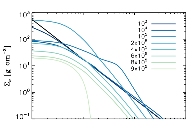
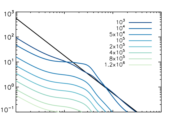
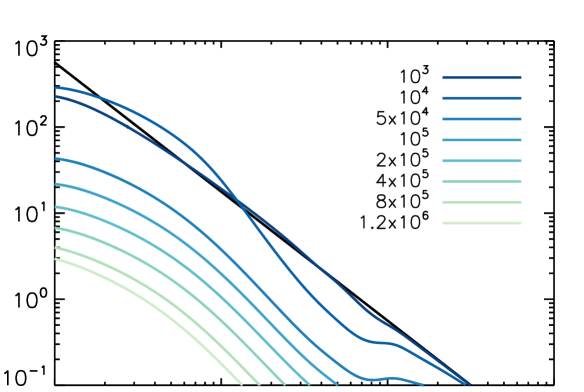
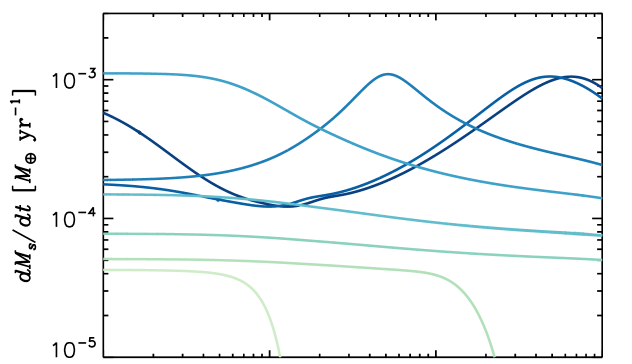
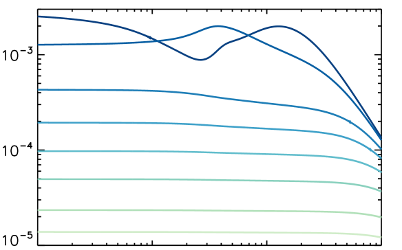
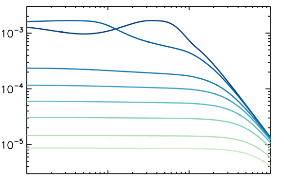
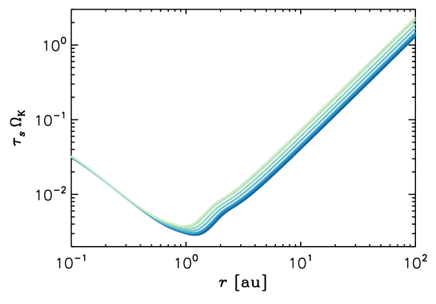
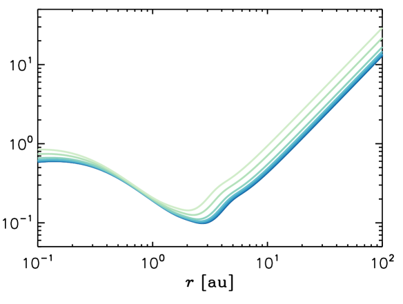
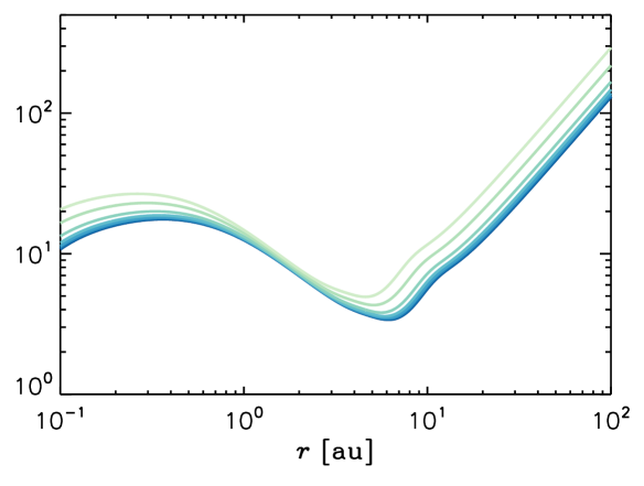
Figure 4: Solutions of Equation (10) for rocky solids of radius $R_{s}$, equal to $1$ (left), $10$ (center), and $100\,\mathrm{cm}$ (right). From top to bottom, panels show $\Sigma_{s}$, $dM_{s}/dt$, and $\tau_{s}\Omega_{\mathrm{K}}$. Times in the legends are in years. The black curves in the top panels represent the initial distribution of solids. See text for further details.

The evolution of solids of a particular size can be obtained by solving Equation (10) for a fixed $R_{s}$. In this case $\tau_{s}\Omega_{\mathrm{K}}$ is a function of both $t$ and $r$, and Equation (2) must be inverted at any time and distance in order to self-consistently determine $\dot{a}_{s}$ and $\tau_{s}$. The evolution of the disk’s gas cannot be neglected in this case. Thus, it is assumed that gas is depleted via accretion on the star and through photo-evaporation by hard radiation from the star. The gas kinematic viscosity is taken as $\nu_{g}\propto 1/\Sigma_{g}$ ($\alpha_{g}\approx 10^{-3}$ at $1\,\mbox{au}$), so that $d(\nu_{g}\Sigma_{g})/dr=0$ and Equation (8) reduces to $u^{r}_{g}=-(3/2)\nu_{g}/r$. For simplicity, the time evolution of $\Sigma_{g}$ is obtained by re-scaling the initial condition (the same as in Figure 3) according to the current gas mass ($\partial\ln{\Sigma_{g}}/\partial\ln{r}$ is constant in time). The disk’s gas is entirely depleted in $\approx 3.5\,\mbox{Myr}$ (e.g., Weiss et al., 2021).

Figure 4 illustrates the evolution for rocky solids of $1$ (left), $10$ (center), and $100\,\mathrm{cm}$ (right) radius. The initial inventory of solids, $\approx 183\,\mbox{$M_{\oplus}$}$, is entirely removed within $\approx 9\times 10^{5}$ years for the case shown in the left panels. The reason is that maximal accretion ($\tau_{s}\Omega_{\mathrm{K}}\approx 1$) is initially sustained at distances of several tens of au, rapidly transferring large amounts of solids toward the star (see top-left and middle-left panels). Consequently, two-thirds of the initial mass is removed in $\approx 3\times 10^{5}$ years. For particles with $R_{s}=10$ and $100\,\mathrm{cm}$, respectively $\approx 60$ and $\approx 110\,\mbox{$M_{\oplus}$}$ are left at $1\,\mbox{Myr}$, but $\lesssim 1\,\mbox{$M_{\oplus}$}$ remains inside $20\,\mbox{au}$. At $t\approx 5\times 10^{5}$ years, $dM_{s}/dt$ inside $100\,\mbox{au}$ ranges from a few to several $10^{-5}\,\mathrm{\mbox{$M_{\oplus}$}\,yr^{-1}}$, dropping below $10^{-5}\,\mathrm{\mbox{$M_{\oplus}$}\,yr^{-1}}$ after $1\,\mbox{Myr}$.

An experiment conducted with $R_{s}=10\,\mathrm{m}$ rocks indicates that over $75$% of the initial solids’ mass survives after $3\,\mbox{Myr}$ (because $\tau_{s}\Omega_{\mathrm{K}}\gg 1$), but only $\approx 5\,\mbox{$M_{\oplus}$}$ orbit within $10\,\mbox{au}$, where $dM_{s}/dt\lesssim 10^{-5}\,\mathrm{\mbox{$M_{\oplus}$}\,yr^{-1}}$ after $10^{5}$ years. Beyond $20\,\mbox{au}$, $dM_{s}/dt$ never exceeds $\approx 10^{-5}\,\mathrm{\mbox{$M_{\oplus}$}\,yr^{-1}}$ during the disk’s evolution.

The bottom panels of Figure 4 indicate that, for $0.1<r<100\,\mbox{au}$, $\tau_{s}\Omega_{\mathrm{K}}$ can vary by up to three orders of magnitude for $R_{s}=1$ and $10\,\mathrm{cm}$ particles and by over an order of magnitude for $R_{s}=1\,\mathrm{m}$ (and $10\,\mathrm{m}$) bodies. The largest particles also display a significant increase of $\tau_{s}$, at any given $r$, as the disk’s gas dissipates. Clearly, the condition $\tau_{s}\Omega_{\mathrm{K}}=\mathrm{constant}$ is only indicative of a particle size for a given gas state. In these examples, $\tau_{s}\Omega_{\mathrm{K}}=1$ corresponds to $R_{s}\approx 1\,\mathrm{cm}$ particles between $r\approx 50$ and $\approx 80\,\mbox{au}$, and to $R_{s}\approx 10\,\mathrm{cm}$ particles between $r\approx 10$ and $\approx 20\,\mbox{au}$. Larger particles (in the $\approx 10$–$100\,\mathrm{cm}$ range) would satisfy this condition inside $10\,\mbox{au}$.

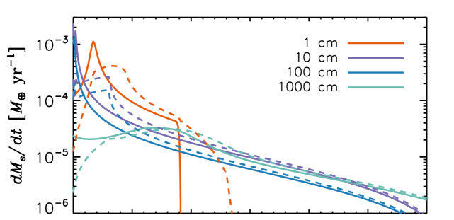
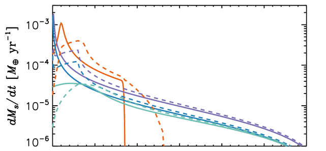
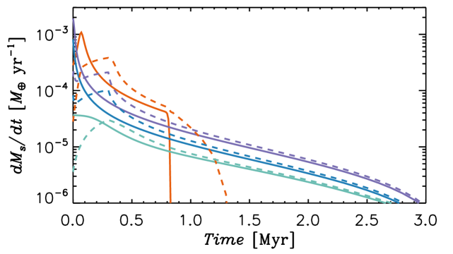
Figure 5: Solutions of Equation (10) for solids of radius $R_{s}$, as indicated, for the accretion rate through the disk, $dM_{s}/dt$. The panels illustrate the evolution at distance $r=1$ (top), $5$ (center), and $10\,\mbox{au}$ (bottom). Solid lines represent results from the disk model in Figure 4. Dashed lines indicate results from similar models with a source term, $\Lambda$ (see text for details).

Figure 5 shows $dM_{s}/dt$ versus time at $r=1$ (top), $5$, and $10\,\mbox{au}$ (bottom), for calculations presented in Figure 4 (solid lines). For the first few $10^{5}$ years, $dM_{s}/dt$ can be $\gtrsim 10^{-4}\,\mathrm{\mbox{$M_{\oplus}$}\,yr^{-1}}$, but it becomes $\lesssim 10^{-5}\,\mathrm{\mbox{$M_{\oplus}$}\,yr^{-1}}$ by $\approx 1\,\mbox{Myr}$. The same calculations were executed applying the source term $\Lambda(t,r)=0.9\,\Sigma_{s}(0,r)/\tau_{c}$ in Equation (10), with a “coagulation time” $\tau_{c}=3\times 10^{5}\,\mathrm{yr}$ (Voelkel et al., 2020) and $\Lambda=0$ for $t>\tau_{c}$. At $t=0$, $10$% of the initial solids’ mass is already in the form of particles of radius $R_{s}$. These latter results are illustrated in Figure 5 as dashed lines. Compared to the solid curves, peaks in $dM_{s}/dt$ are lower and broader, but differences become small after $\approx 0.5\,\mbox{Myr}$. Results presented in Figures 3-5 are approximate but representative of the evolution of the solids’ density and accretion rates in an unperturbed disk.

2.2 Dynamics in Perturbed Disks

In the presence of a perturbing body, e.g., a planet, Equation (9) can be interpreted as the rate at which solids can be supplied to the proximity of its orbit, thus determining the maximum rate of solids’ accretion on the planet. Assume that the thickness of the disk of solids, $H_{s}$, is infinitesimal, then the accretion rate on a small planet is essentially two-dimensional and can be approximated by

$$\frac{d\mbox{$M_{p}$}}{dt}\approx\frac{1}{\pi}\left(\frac{R_{\mathrm{eff}}}{a_{p}}\right)\frac{dM_{s}}{dt},$$ (11)

in which $M_{p}$ and $a_{p}$ are the planet mass and orbital radius, respectively. This expression assumes that the mass flux of solids in the radial direction can be approximated as azimuth-independent, so that the fraction of the integrated flux intercepted by the planet is given by the ratio of the planet “effective” size to the orbit circumference. This approximation is useful when working in one-dimensional, radial disks. Corrections due to azimuthal variations of the solid’s transport can be accounted for in the definition of the planet’s effective radius for accretion. In fact, the radius $R_{\mathrm{eff}}$ can be much larger than the planet’s physical radius, $R_{p}$ (the two-dimensional assumption implies that $R_{\mathrm{eff}}>H_{s}$).

Applying a formalism developed for the accretion of planetesimals in the two-body problem framework (see, e.g., Lissauer, 1987), the effective radius for capture of solids can be written as $R_{\mathrm{eff}}\approx R_{p}(u_{\mathrm{esc}}/u_{\mathrm{rel}})$, if $u_{\mathrm{esc}}\gg u_{\mathrm{rel}}$ (otherwise $R_{\mathrm{eff}}\approx R_{p}$), where $u_{\mathrm{esc}}=\sqrt{2G\mbox{$M_{p}$}/R_{p}}$ is the escape velocity from the planet surface and $u_{\mathrm{rel}}$ is the relative velocity (in magnitude) between the planet and the solids. This relation originates from conservation of relative energy and angular momentum of the approaching particle. If $\tau_{s}\Omega_{\mathrm{K}}\gg\alpha_{g}$, the relative velocity can be obtained directly from Equations (5) and (6),

$$u_{\mathrm{rel}}\approx\left(\frac{H_{g}}{a_{p}}\right)^{2}\frac{\sqrt{1/4+(\tau_{s}\Omega_{\mathrm{K}})^{2}}}{1+(\tau_{s}\Omega_{\mathrm{K}})^{2}}\Omega_{\mathrm{K}}a_{p},$$ (12)

assuming that planet is on circular orbit.

The efficiency, or probability, of accretion of solids onto a planet is defined as

$$\zeta=\frac{\dot{M}_{p}}{\dot{M}_{s}},$$ (13)

where $\dot{M}_{s}$ is the accretion rate of solids toward the planet, in the proximity of its orbit (and $\dot{M}_{p}\leq\dot{M}_{s}$ by assumption). Inserting the effective radius given above in Equation (11), we find

$$\zeta\approx\frac{\sqrt{2}}{\pi}\!\left(\frac{a_{p}}{H_{g}}\right)^{2}\!\!\frac{1+(\tau_{s}\Omega_{\mathrm{K}})^{2}}{\sqrt{1/4+(\tau_{s}\Omega_{\mathrm{K}})^{2}}}\sqrt{\!\left(\frac{\mbox{$M_{p}$}}{\mbox{$M_{\star}$}}\right)\!\!\left(\frac{R_{p}}{a_{p}}\right)},$$ (14)

in which $M_{\star}$ is the stellar mass. For $\tau_{s}\Omega_{\mathrm{K}}\gtrsim 1$, Equation (14) scales with planet mass and stopping time as the accretion probability estimated by Kary et al. (1993) in the “non-gravitating” planet limit, $\zeta\propto\tau_{s}\Omega_{\mathrm{K}}\mbox{$M_{p}$}^{2/3}\propto\tau_{s}\Omega_{\mathrm{K}}(\mbox{$R_{\mathrm{H}}$}/a_{p})^{2}$, where $R_{\mathrm{H}}$ is the Hill radius of the planet. Maximum values of the large-scale transport of solids, i.e., $dM_{s}/dt$ in Equation (9), occur when $\tau_{s}\Omega_{\mathrm{K}}\approx 1$, at which $\zeta\approx(4/\pi)(a_{p}/H_{g})^{2}\sqrt{(2/5)(\mbox{$M_{p}$}/\mbox{$M_{\star}$})(R_{p}/a_{p})}$. For a Moon-size planetary embryo orbiting at $5\,\mbox{au}$, the efficiency would be $\approx 10^{-4}$. Therefore, the values of $dM_{s}/dt$ reported in Figure 5 would result in $d\mbox{$M_{p}$}/dt<10^{-7}\,\mbox{$M_{\oplus}$}\,\mathrm{yr^{-1}}$, and in a mass-doubling timescale exceeding $10^{5}$ years.

Alternatively, the effective radius for the capture of solids can be estimated by equating the gravitational and relative kinetic energies (Lambrechts & Johansen, 2012), a condition required for escape, resulting in $R_{\mathrm{eff}}\approx 2G\mbox{$M_{p}$}/u^{2}_{\mathrm{rel}}$. By using Equation (12), this approximation yields an efficiency

$$\zeta\approx\frac{2}{\pi}\!\left(\frac{a_{p}}{H_{g}}\right)^{4}\frac{\left[1+(\tau_{s}\Omega_{\mathrm{K}})^{2}\right]^{2}}{1/4+(\tau_{s}\Omega_{\mathrm{K}})^{2}}\left(\frac{\mbox{$M_{p}$}}{\mbox{$M_{\star}$}}\right).$$ (15)

In this case, a Moon-size embryo orbiting at $5\,\mbox{au}$ would have $\zeta\approx 10^{-2}$ at maximum values of $dM_{s}/dt$ ($\tau_{s}\Omega_{\mathrm{K}}\approx 1$), hence $d\mbox{$M_{p}$}/dt\lesssim 10^{-5}\,\mbox{$M_{\oplus}$}\,\mathrm{yr^{-1}}$, much larger than the previous assessment. However, both approximations for the effective radius neglect stellar gravity, which implies that in neither case $R_{\mathrm{eff}}$ can exceed $\approx\mbox{$R_{\mathrm{H}}$}$, hence $\zeta\lesssim(\mbox{$R_{\mathrm{H}}$}/a_{p})/\pi$. The accretion efficiency of a Moon-mass body would therefore be limited to $\approx 10^{-3}$. The remainder of the difference between the estimates provided by Equation (14) and (15) can be resolved by applying a more appropriate evaluation of $u_{\mathrm{rel}}$ close to the planet, as explained below.

If $R_{\mathrm{eff}}\lesssim H_{s}$, the two-dimensional approximation for accretion of solids breaks down and the right-hand side of Equation (11), hence the efficiency $\zeta$ (see Equation (13)), must be multiplied by $(\pi/4)(R_{\mathrm{eff}}/H_{s})$. In the small-particle regime, the thickness $H_{s}$ can be affected by turbulent stirring. If the kinematic viscosity $\nu_{g}$ is written in terms of $\alpha_{g}$, then (Dubrulle et al., 1995)

$$\frac{H_{s}}{H_{g}}\approx\sqrt{\frac{\alpha_{g}}{\alpha_{g}+2\tau_{s}\Omega_{\mathrm{K}}}},$$ (16)

where the numerical factor depends on the nature of turbulence (and may be somewhat different from $2$, see discussion in Dubrulle et al., 1995). Typical values of the turbulence parameter $\alpha_{g}\sim 10^{-4}$–$10^{-2}$ would result in $H_{s}/H_{g}\sim 0.01$–$0.1$ for $\tau_{s}\Omega_{\mathrm{K}}\approx 1$ (see also Lambrechts & Johansen, 2012). Since gas temperatures in planet-forming regions correspond to $H_{g}/a_{p}\sim 0.01$–$0.1$ (e.g., D’Alessio et al., 1998), the relative thickness of the solid layer would be $H_{s}/a_{p}\sim 10^{-4}$–$10^{-2}$. Thus, in the two-dimensional accretion regime (i.e., $R_{\mathrm{eff}}>H_{s}$) $\zeta>(1/\pi)H_{s}/a_{p}$, and thus, $\gtrsim 10^{-5}$–$10^{-3}$ for $\tau_{s}\Omega_{\mathrm{K}}\approx 1$.

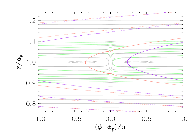
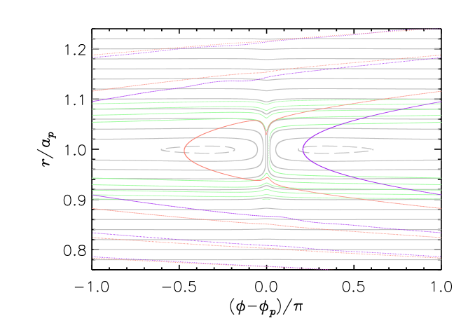
Figure 6: Trajectories in the rotating frame of the planet of $R_{s}=1$ (green), $10$ (orange), and $100\,\mathrm{cm}$ (purple) particles, orbiting in a disk perturbed by a $5$ (top) and a $15\,\mbox{$M_{\oplus}$}$ planet (bottom) on circular orbits. The trajectory of the smallest particle is initiated as the others but a smaller portion is plotted. Gray lines represent streamlines of the perturbed gas. The unperturbed disk properties are as in Figure 1 at $5\,\mbox{au}$ (see also Table 1).

Equations (14) and (15) neglect the gravitational perturbations exerted by the planetary body, which alter the dynamics of both solids and gas, i.e., $u_{\mathrm{rel}}$ is different from the unperturbed expression derived from Equations (5) and (6). An approximation to the perturbed rotation rate of the gas is still given by Equation (3), in which $\Phi$ must comprise the contributions due to the planet, including non-inertial terms (if applicable), i.e.,

$$\Phi=-\frac{G\mbox{$M_{\star}$}}{r}-\frac{G\mbox{$M_{p}$}}{|\boldsymbol{r}-\boldsymbol{r}_{p}|}+\frac{G\mbox{$M_{p}$}}{r_{p}^{3}}\,\boldsymbol{r}\!\boldsymbol{\cdot}\!\boldsymbol{r}_{p},$$ (17)

where $\boldsymbol{r}$ and $\boldsymbol{r}_{p}$ are the generic and planet position vectors. Neglecting contributions from gas pressure variations along the azimuthal direction around the star, the perturbed radial component of the gas velocity is (Ogilvie & Lubow, 2006)

$$u^{r}_{g}\approx-\left(\frac{2}{r\Omega_{\mathrm{K}}}\right)\frac{\partial\Phi}{\partial\phi},$$ (18)

in which $\phi$ is the azimuthal angle. The radial velocity arising from global transport, Equation (8), should be added to the right-hand side of Equation (18), if relevant. Given the importance of gas drag, corrections to the gas flow introduced by Equations (3), (17) and (18) can have non-trivial effects on the dynamics of small solids.

The perturbed gas velocity can be used to integrate the trajectories of solid particles through the disk (see, e.g., DP15, ). Some examples are shown in Figure 6, in a frame co-rotating with the planet, for $R_{s}=1$ (green line), $10$ (orange line), and $100\,\mathrm{cm}$ rocky particle (purple line) drifting through the gas perturbed by $5$ (top) and $15\,\mbox{$M_{\oplus}$}$ planets (bottom) on circular orbits. The gray lines represent perturbed gas streamlines. The particle motion is altered by the planet’s gravity and by drag forces due to the perturbed gas velocity field, invalidating the approximations applied in deriving Equations (5) and (6). Those equations remain valid only sufficiently far from the orbit of the planet. Note that this approach does not account for planet-induced tidal perturbations on the gas density, and hence pressure, which can also affect particle dynamics, as discussed later, and are expected to become increasingly important as $M_{p}$ grows.

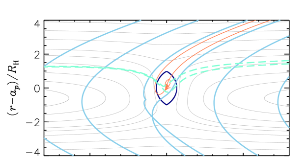
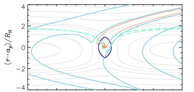
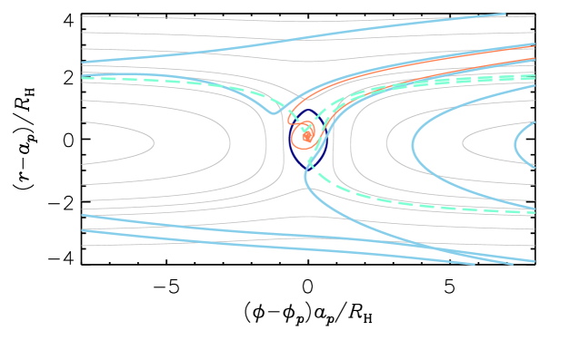
Figure 7: Trajectories of $R_{s}=1$ (dashed lines) and $30\,\mathrm{cm}$ (solid lines) rocky particles in the proximity of $0.01$ (top), $0.1$, and $1\,\mbox{$M_{\oplus}$}$ (bottom) planets, orbiting at $a_{p}=5\,\mbox{au}$ on circular orbits. Trajectories are represented in a frame co-rotating with the planet. Gray lines represent gas streamlines. The planet’s Roche lobe is also shown. The unperturbed disk properties are as in Figure 1 at $5\,\mbox{au}$ ($\tau_{s}\Omega_{\mathrm{K}}\approx 1$ for $R_{s}=30\,\mathrm{cm}$ and $\approx 10^{-2}$ for $R_{s}=1\,\mathrm{cm}$).

Figure 7 illustrates results from similar experiments, at lower masses: $\mbox{$M_{p}$}=0.01$ (top), $0.1$, and $1\,\mbox{$M_{\oplus}$}$ (bottom) at $a_{p}=5\,\mbox{au}$. The particle radius is $R_{s}=1$ (dashed lines) and $30\,\mathrm{cm}$ (solid lines), corresponding respectively to $\tau_{s}\Omega_{\mathrm{K}}\approx 0.01$ and $\approx 1$ for the disk conditions at $5\,\mbox{au}$ in Figure 1. Gas streamlines are also plotted, along with the Roche lobe contours in the disk mid-plane. The calculation of the Roche lobe contours neglects modifications induced by gas drag (Murray, 1994). The numerical results indicate that the estimate of $R_{\mathrm{eff}}$ used in Equation (14) may be a reasonable approximation in these cases. Although the accretion stream entering the Roche lobe is asymmetric with respect to the planet (see orange trajectories), an average size of $R_{\mathrm{eff}}$ can be estimated as a few tenths of $R_{\mathrm{H}}$. An outcome similar to that of the $R_{s}=30\,\mathrm{cm}$ particles is obtained from the trajectory of $R_{s}=100\,\mathrm{cm}$ particles (not shown). In these experiments, the particle trajectories are integrated until they impact the planet, assumed to be a condensed object. As argued below, an atmosphere could extend at most over some fraction of the Bondi radius, $\lesssim 0.2\,\mbox{$R_{\mathrm{H}}$}$ in the $\mbox{$M_{p}$}=1\,\mbox{$M_{\oplus}$}$ case (and much less in the other cases), a length $\lesssim R_{\mathrm{eff}}$.

It must be pointed out that, in the presence of a perturbing body, the unperturbed relative velocity provided by Equation (12), which is independent of the distance $\widetilde{r}$ from the perturbing object and of its mass $M_{p}$, is appropriate for use only far away from the perturber. However, both Equation (14) and Equation (15) neglect three-body effects, and therefore the relative velocity should be sampled where the gravity field of the planetary body dominates, that is, where gravitational perturbations on $u_{\mathrm{rel}}$ are non-negligible. If $\tau_{s}\Omega_{\mathrm{K}}\ll 1$, the perturbed relative velocity can be estimated from Equations (3), (17) and (18), and depends on $M_{p}$, $\widetilde{r}$, and the direction of approach. At a distance $\widetilde{r}\approx\mbox{$R_{\mathrm{H}}$}$, its magnitude is roughly $\propto\mbox{$R_{\mathrm{H}}$}$ and, for Moon-mass bodies, it is several times as large as the unperturbed velocity predicted by Equation (12). For finite (non-zero) values of the particle stopping time, analytical derivations of the perturbed velocity are more involved, but it can be easily evaluated through numerical integration of trajectories (as in Figure 7). For $\tau_{s}\Omega_{\mathrm{K}}\approx 1$, such experiments indicate that particles approaching a Moon-mass body can achieve relative velocities many times (up to a factor of ten) as large as Equation (12) at distances $\widetilde{r}\lesssim\mbox{$R_{\mathrm{H}}$}$. Applying this correction, the efficiencies predicted by Equation (14) and (15) become similar.

2.3 Simple Estimates of Accretion Efficiencies

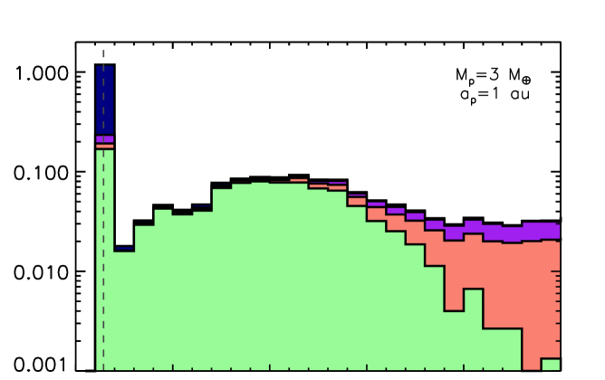
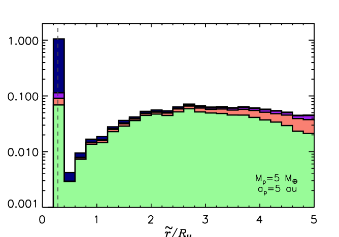
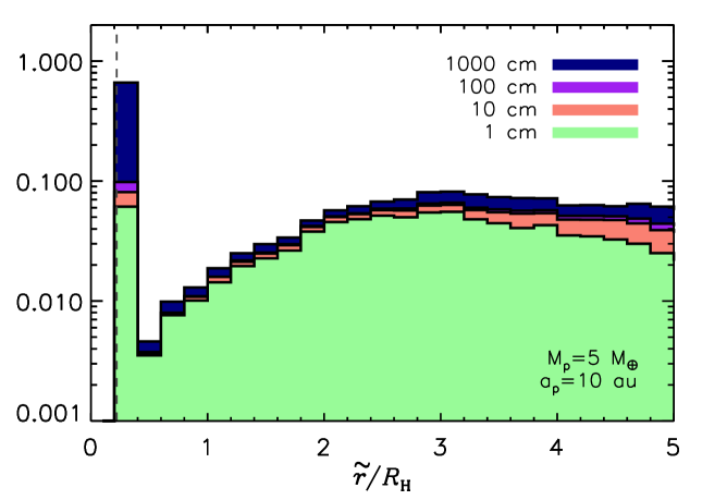
Figure 8: Histograms of the closest approach, in units of the planet’s Hill radius, along the trajectories of $R_{s}=1$, $10$, $100$, and $1000\,\mathrm{cm}$ particles (as indicated). Each bin is normalized by the total mass used in the experiment for the given particle size. Bins are stacked in order of increasing $R_{s}$, rendered by different colors. The dashed line indicates the planet’s Bondi radius. The unperturbed disk properties correspond to those of Figure 1, according to $a_{p}$. The case at $1\,\mbox{au}$ (top panel) uses the highest gas density in Figure 1.

The approach used for the trajectory integration in Figures 6 and 7 is applied to conduct experiments on the accretion of particles, with radii of $1$, $10$, $100$, and $1000\,\mathrm{cm}$, on $\mbox{$M_{p}$}=3$ and $5\,\mbox{$M_{\oplus}$}$ planets orbiting at $a_{p}=1$, $5$, and $10\,\mbox{au}$. These experiments provide a statistical estimate of the accretion efficiency $\zeta$ for the simplified gas flow given by Equations (3), (17) and (18). The gas density is axisymmetric around the star and proportional to a power of $r$. A summary of the results is displayed in Figure 8. Histograms of the closest approach distance along the particles’ trajectories for the $\mbox{$M_{p}$}=3\,\mbox{$M_{\oplus}$}$ planet at $a_{p}=1\,\mbox{au}$ (top panel) and for the $\mbox{$M_{p}$}=5$ planets at $a_{p}=5$ and $10\,\mbox{au}$ (center and bottom panels, respectively, see also figure’s caption). The gas densities are those quoted in Figure 1 (see also Table 1), according to the planet’s orbital radius (at $a_{p}=1\,\mbox{au}$, $\Sigma_{g}\approx 1100\,\mbox{$\mathrm{g\,cm}^{-2}$}$). All trajectories begin as random circles at radial distances beyond the 2:3 mean-motion resonance with the planet, out to a distance somewhat beyond the 1:2 resonance (in the orbital plane of the planet). These experiments assume equal masses of icy and rocky particles, in each size bin, at $a_{p}=5$ and $10\,\mbox{au}$, and only rocks at $a_{p}=1\,\mbox{au}$. Accretion is occurs if a particle enters the planetary envelope, $\widetilde{r}<R_{p}$ and $R_{p}$ is taken as the Bondi radius, Equation (19). For a solid to be permanently captured, its relative velocity in the envelope must not exceed the escape velocity, $u_{\mathrm{esc}}$. These experiments do not account for such requirement, which is generally irrelevant for the small particles considered here (as confirmed by the calculations discussed in Section 3).

The closest approach distance from the planet in Figure 8 is in units of $R_{\mathrm{H}}$. For a given particle radius, the histogram bins are normalized to indicate the fraction of the initial mass of the solids with radius $R_{s}$ considered in the experiment. Bins are then overlaid in order of increasing solid size. The vertical dashed line indicates the distance $\widetilde{r}=\mbox{$R_{\mathrm{B}}$}$, the assumed envelope radius. Consistently with the results of Figure 7, the histograms show that particles of all sizes can enter the planet’s Hill sphere without necessarily being captured. The pile-up in the bin interior to or overlapping $R_{p}$ is caused by particles flagged as accreted. Since each color represents a normalized mass, the innermost bin in each panel provides a measure of the efficiency $\zeta$, estimated here as the accreted mass divided by the mass of solids approaching and interacting with the planet.

Particles with an initial $\tau_{s}\Omega_{\mathrm{K}}\sim 1$ have $R_{s}\approx 10$–$100\,\mathrm{cm}$. For both planet masses, the efficiency ranges from a few to several percent. For $1\,\mathrm{cm}$ particles ($\tau_{s}\Omega_{\mathrm{K}}\lesssim 10^{-2}$ initially), $\zeta$ ranges from a few to $\approx 15$%. The largest, $1000\,\mathrm{cm}$ particles ($\tau_{s}\Omega_{\mathrm{K}}>10^{2}$ initially) can accrete efficiently: $\zeta>50$% in these experiments. For the two $\mbox{$M_{p}$}=5\,\mbox{$M_{\oplus}$}$ cases, $\zeta$ is comparable across the entire range of particle sizes.

An estimate of the accretion rate of solids, $\dot{M}_{p}=\zeta\dot{M}_{s}$, can be obtained by combining the results in Figures 5 and 8. The mass flux of $R_{s}=1\,\mathrm{cm}$ particles is sustained over the first $\approx 0.5\,\mbox{Myr}$ ($\dot{M}_{s}\sim 10^{-4}\,\mathrm{\mbox{$M_{\oplus}$}\,yr^{-1}}$), producing values of $\dot{M}_{p}$ in the range $10^{-6}$–$10^{-5}\,\mathrm{\mbox{$M_{\oplus}$}\,yr^{-1}}$. Particles with $R_{s}=10$–$100\,\mathrm{cm}$ have low $\zeta$ which, compounded with $\dot{M}_{s}\sim 10^{-5}\,\mathrm{\mbox{$M_{\oplus}$}\,yr^{-1}}$ over the first $1\,\mbox{Myr}$, would result in $\dot{M}_{p}$ of order $10^{-7}$–$10^{-6}\,\mathrm{\mbox{$M_{\oplus}$}\,yr^{-1}}$. During the first $1\,\mbox{Myr}$, $R_{s}=1000\,\mathrm{cm}$ solids also have $\dot{M}_{s}\sim 10^{-5}\,\mathrm{\mbox{$M_{\oplus}$}\,yr^{-1}}$, which would generate values of $\dot{M}_{p}$ up to $\sim 10^{-5}\,\mathrm{\mbox{$M_{\oplus}$}\,yr^{-1}}$. It is important to notice that high values of $\zeta$ for a particular solid size imply an efficient removal of these solids, which then cannot significantly contribute to the growth of other planets orbiting closer to the star.

A number of effects are neglected in these experiments. Gas density perturbations driven by the planet’s tidal field can impact the drag forces exerted on the particles, possibly causing a size-dependent segregation effect. Additionally, the complex three-dimensional flow circulation in the proximity of the planet can alter the balance of forces and change the outcome of the capture process. Moreover, for the icy solids, variations of the gas temperature close to the planet can promote ablation and vaporize some fraction of the local mass of solids. These effects, which require more realistic disk-planet interaction models and more sophisticated calculations of the solids’ evolution in disks, are included in the simulations discussed below.

3 Radiation-Hydrodynamics Calculations of Solids’ Accretion

3.1 Gas Thermodynamics

Table 1: Properties of Planets and Disks in the RHD Models

$a_{p}$ [au]	$\mbox{$M_{p}$}/\mbox{$M_{\oplus}$}$	$\mbox{$R_{\mathrm{B}}$}/a_{p}$	$R_{p}/\mbox{$R_{\mathrm{B}}$}$	$R_{p}/\mbox{$R_{\mathrm{H}}$}$	$\langle T_{g}\rangle$ [$\mathrm{K}$]	$\langle\rho_{g}\rangle$ [$\mathrm{g\,cm}^{-3}$]
$10$	0$5$	$0.0038$	$0.69$	$0.15$	0$80$	$5.0\times 10^{-12}$
$10$	$10$	$0.0075$	$0.48$	$0.17$
$10$	$15$	$0.0113$	$0.40$	$0.18$
0$5$	0$5$	$0.0050$	$0.92$	$0.27$	$124$	$1.3\times 10^{-11}$
0$5$	$10$	$0.0097$	$0.67$	$0.30$
0$5$	$15$	$0.0150$	$0.64$	$0.39$
0$1$	0$3$	$0.0091$	$1.00$	$0.61$	$200$	$2.0\times 10^{-11}$
0$1$	0$3$	$0.0055$	$1.00$	$0.37$	$330$	$1.5\times 10^{-10}$
0$1$	0$3$	$0.0039$	$1.00$	$0.26$	$470$	$6.7\times 10^{-10}$
0$1$	$20$	$0.0602$	$0.32$	$0.70$	$200$	$2.0\times 10^{-11}$
0$1$	$20$	$0.0365$	$0.52$	$0.70$	$330$	$1.5\times 10^{-10}$
0$1$	$20$	$0.0256$	$0.74$	$0.70$	$470$	$6.7\times 10^{-10}$

During the relatively rapid motion of small particles through the disk, disk’s gas can be assumed to be in a quasi-steady state, so that its thermodynamic fields, e.g., velocity $\boldsymbol{u}_{g}$, temperature $T_{g}$, and density $\rho_{g}$, remain nearly constant in time when described in a reference frame co-rotating with an embedded planet on a circular orbit. This assumption is based on the fact that global disk evolution is mainly driven by viscous transport during the stages considered here. This study uses the thermodynamic steady-state fields $(\boldsymbol{u}_{g},\rho_{g},T_{g})$ from the models of D’Angelo & Bodenheimer (2013, hereafter DB13), who performed global three-dimensional (3D) radiation-hydrodynamics (RHD) calculations of planets embedded in disks. They modeled planets of mass $\mbox{$M_{p}$}=5$, $10$, and $15\,\mbox{$M_{\oplus}$}$ on circular orbits at $a_{p}=5$ and $10\,\mbox{au}$ from a solar-mass star. In all cases, the envelope mass was a small fraction of $M_{p}$. Table 1 lists some properties of these models.

Briefly, DB13 adopted a spherical polar discretization of the disk, with coordinates $\{r,\theta,\phi\}$, solving the Navier-Stokes equations for a compressible and viscous fluid in a reference frame rotating about the star at the same angular velocity as the planet’s orbital frequency. They applied a numerical method that is effectively second-order accurate in both space and time (see, e.g., Boss & Myhill, 1992). The disks extended in radius from $0.5\,a_{p}$ to $2\,a_{p}$, about $15^{\circ}$ in the meridional direction, and $2\pi$ radians in azimuth around the star. The energy equation accounted for advection of gas and radiation energy, work done by gas and radiation pressure, viscous dissipation, radiation transport, and energy released by accreted solids. Radiative transfer was approximated via flux-limited diffusion (Levermore & Pomraning, 1981; Castor, 2007) and solved by means of an implicit algorithm second-order accurate in both space and time (an approach recently validated by Bailey et al., 2023). The gas equation of state was that of a mixture of hydrogen and helium in solar proportions that accounted for ionization of atomic species, dissociation of molecular hydrogen, and for the translational, rotational, and vibrational energy states of H₂.

Once a thermodynamic quasi-steady state has been achieved, as in the models of DB13, the disk evolution proceeds on the viscous timescale, $\sim r^{2}/\nu_{g}$. The calculations adopted a turbulent viscosity parameter $\alpha_{g}\approx 10^{-3}$, corresponding to a viscous timescale several $10^{4}$ orbital periods at $r=a_{p}$. This level of turbulence is in accord with observational estimates (e.g., Flaherty et al., 2018). Toward the end of a disk’s lifetime, when gas density is very low, evolution is mainly driven by stellar photo-evaporation and the gas is cleared inside-out (e.g., Gorti et al., 2009; Ercolano & Pascucci, 2017).

For the purposes of this study, an important aspect of DB13’s models is that they are global (disks extend many au in radius), and resolve the actual envelopes of the planetary cores. They did so by applying hierarchies of nested grids with finest resolutions comparable to the condensed core radii. In fact, a detailed comparison was performed between 3D envelopes and one-dimensional, spherically symmetric envelopes obtained from planet structure and evolution calculations. The high resolution of the models allows the trajectories of solids to be integrated until they enter the actual planetary envelopes.

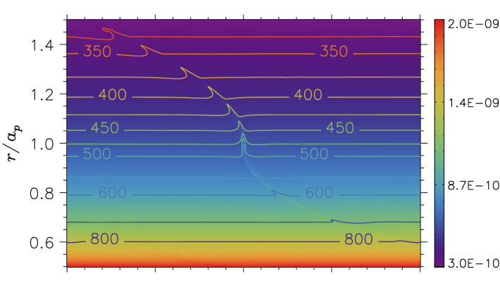
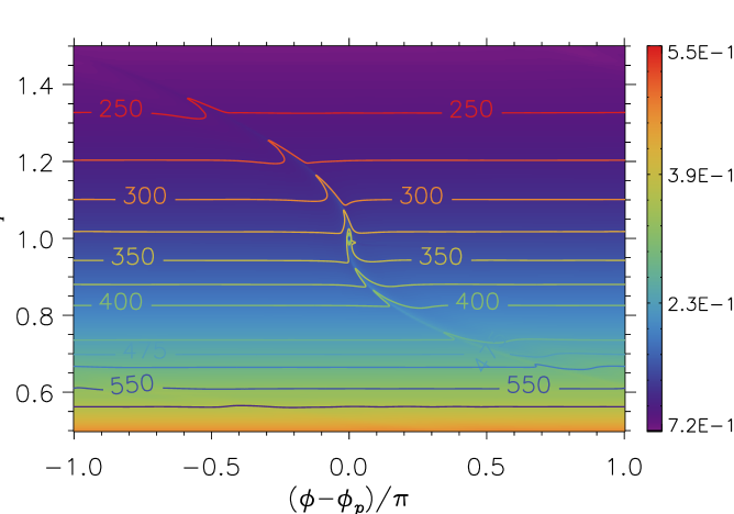
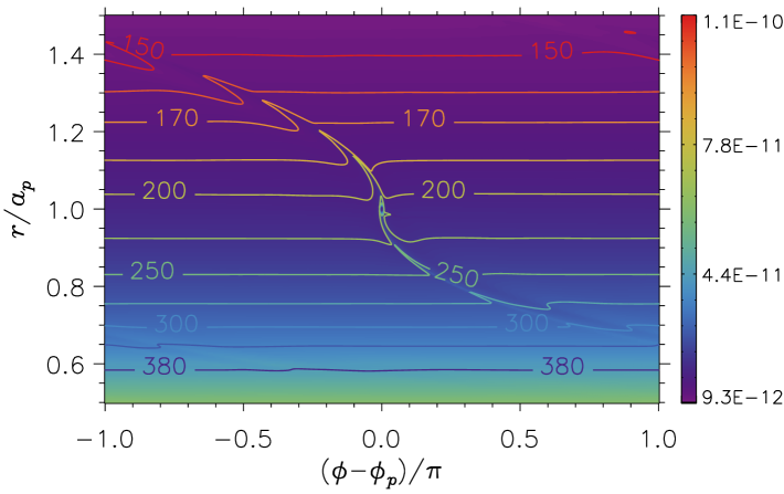
Figure 9: Steady-state gas density (color scale) and temperature (contour lines) at the disk’s mid-plane, perturbed by a (circular-orbit) $3\,\mbox{$M_{\oplus}$}$ planet located at $r/a_{p}=1$ and $\phi=\phi_{p}$. The density is in units of $\mathrm{g\,cm}^{-3}$ and the temperature in kelvin. The azimuthally-averaged surface density at $r=a_{p}$ is $\Sigma_{g}\approx 1100$ (top), $\approx 220$ (center), and $\approx 20\,\mbox{$\mathrm{g\,cm}^{-2}$}$ (bottom). See also Table 1.

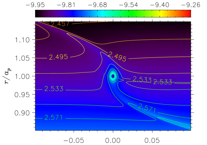
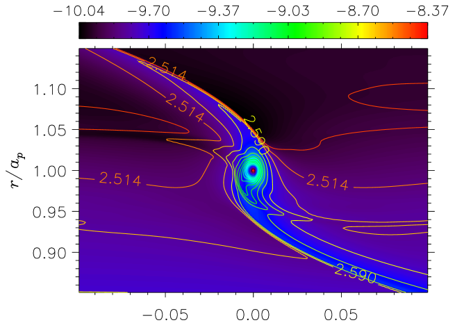
Figure 10: Close-up of $\log{\rho_{g}}$ (color scale) and $\log{T_{g}}$ (contour lines), at the disk’s mid-plane, for the $3$ (top) and $20\,\mbox{$M_{\oplus}$}$ planet (bottom) located at $a_{p}=1\,\mbox{au}$. Gas density and temperature are in units of $\mathrm{g\,cm}^{-3}$ and $\mathrm{K}$, respectively. The unperturbed surface density at $r=a_{p}$ is $\Sigma_{g}\approx 220\,\mbox{$\mathrm{g\,cm}^{-2}$}$.

Models with planets at $a_{p}=5$ and $10\,\mbox{au}$ are complemented by additional RHD calculations of $\mbox{$M_{p}$}=3$ and $20\,\mbox{$M_{\oplus}$}$ planets orbiting at $a_{p}=1\,\mbox{au}$ from a $1\,\mbox{$M_{\odot}$}$ star. In these cases, however, the gas density is varied to mimic different epochs of the disk’s evolution. Values of $\Sigma_{g}$ at $r=a_{p}$ vary from $\approx 20$ to $\approx 1100\,\mbox{$\mathrm{g\,cm}^{-2}$}$ (see Table 1). Steady-state gas density and temperature in the disk’s mid-planes of $a_{p}=1\,\mbox{au}$ models are illustrated in Figure 9. Contrary to the calculations of DB13, these models do not resolve in detail possible gaseous envelopes bound to the cores. Therefore, the planetary cores are assumed to bear an envelope whose radius is the smaller of $R_{\mathrm{B}}$ and $R_{\mathrm{H}}$. Under this assumption, $R_{p}$ in these six models ranges from two to ten times the linear resolution of the grid. A close-up around the planets is illustrated in Figure 10. As a reference, $\mbox{$R_{\mathrm{H}}$}/a_{p}\approx 0.015$ and $0.027$ in the top and bottom panel, respectively.

When the envelope volume is determined by an energy balance rather than by gravity, $R_{p}$ is comparable to the Bondi radius (see Table 1). This distance is found by equating the thermal velocity of the gas around the planetary core and its escape velocity from the core,

$$\mbox{$R_{\mathrm{B}}$}=\left(\frac{\pi}{4}\right)\frac{G\mbox{$M_{p}$}\mu_{g}m_{\mathrm{H}}}{k_{\mathrm{B}}\langle T_{g}\rangle},$$ (19)

where $m_{\mathrm{H}}$ and $k_{\mathrm{B}}$ are standard physical constants, $\mu_{g}$ is the mean molecular weight of the gas mixture, and $\langle T_{g}\rangle$ is the average gas temperature at the disk’s mid-plane and $r=a_{p}$. Equation (19) is valid when the energy of the gas is dominated by thermal energy. However, in the $20\,\mbox{$M_{\oplus}$}$ planet models, $R_{\mathrm{B}}$ is similar (warmest disk model) or exceeds $R_{\mathrm{H}}$. Therefore, in those three cases, it is assumed that $R_{p}=0.7\mbox{$R_{\mathrm{H}}$}$, the mean volume radius of the Roche lobe (Eggleton, 1983). The planetary radii in the models, compared to $R_{\mathrm{B}}$ and $R_{\mathrm{H}}$, are reported in Table 1 (see also Kuwahara & Kurokawa, 2024, for a comparison).

The approach of simulating the evolution of the solids in the gas steady-state fields is dictated by the computational cost of these RHD calculations, which can hardly be executed along with the thermodynamic evolution of solids for the required timescales. Nonetheless, the validity of this approach is tested in Appendix A, where results from two RHD calculations are compared. In the first calculation, a population of small solids evolves in the 3D steady-state fields $(\boldsymbol{u}_{g},\rho_{g},T_{g})$ of a disk, as described in this section. In the second, the same population evolves together with the disk’s gas, starting from the steady-state fields used in the first calculation. As discussed in the Appendix, the outcomes of the two approaches are statistically consistent, with relative differences in accretion rates $\lesssim 10$% and typically hovering around a few percent.

3.2 Thermodynamics of Solids

The physical model for the thermodynamic evolution of the solids is described in DP15. Briefly, the equations of motion of a solid particle are written in terms of its linear and absolute angular momenta per unit mass. The particle is subjected to gravitational forces by the star and the planet, to non-inertial forces, to aerodynamic drag, and to the effect of mass loss due to ablation. The particle temperature, $T_{s}$, is determined through an energy equation that takes into account the work done by gas drag, the energy absorbed from the radiation field of the ambient gas, and black body emission from the particle’s surface. The energy equation also accounts for the energy removed/supplied during phase transitions of the particle’s outer layers. Details on the numerical methods and tests can be found in DP15.

Two types of material are considered here: ice (H₂O) and rock (SiO₂). Particles can lose mass by ablation. In this study, the saturated vapor pressure, $P_{v}$, of SiO₂ is upgraded to that reported by Melosh (2007)

$$\ln\left(\frac{P_{v}}{P_{\mathrm{cr}}}\right)=A\left(1-\frac{T_{\mathrm{cr}}}{T_{s}}\right),$$ (20)

where the critical pressure is $P_{\mathrm{cr}}=1.89\times 10^{9}\,\mathrm{dyne\,cm^{-2}}$, the critical temperature is $T_{\mathrm{cr}}=5398\,\mbox{$\mathrm{K}$}$ and $A=10.675270434$. The temperature of the solid $T_{s}$ is defined in DP15. Ablation in the disk’s gas is important for ice (or an admixture of ice and rock), but much less for rock owing to low gas temperatures. Ablation of rock becomes significant only inside the planetary envelopes, when particles are already accreted.

3.3 Distributions and Segregation of Solids

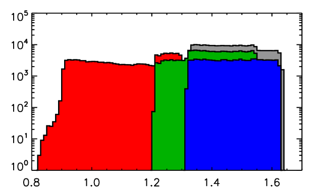
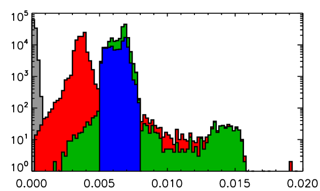
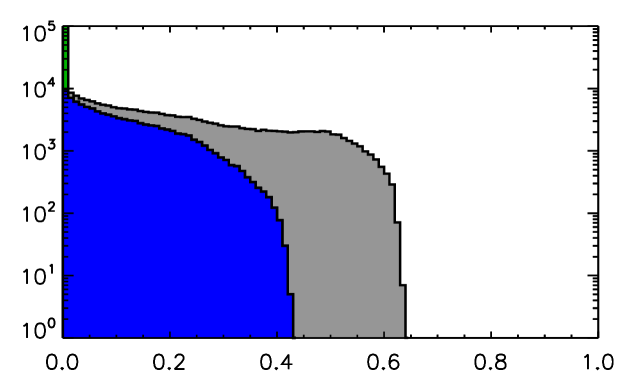
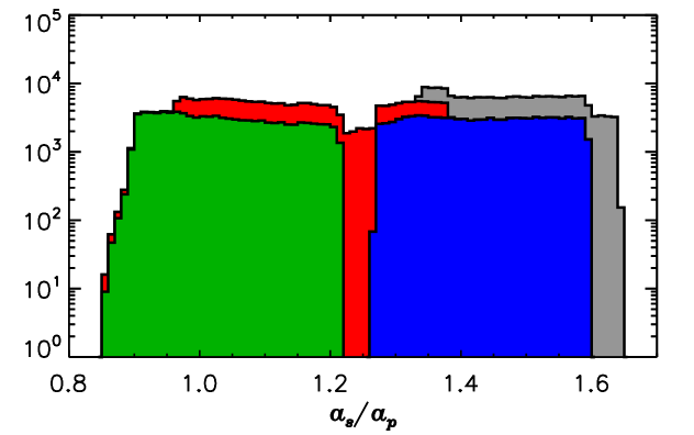
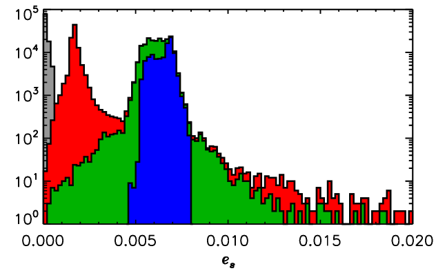
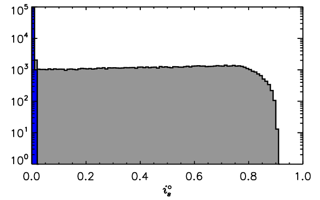
Figure 11: Histograms of the particles’ semi-major axes (left), eccentricities (center) and inclinations (right) as they approach and cross the planet’s orbit ($a_{p}=5\,\mbox{au}$ and $\mbox{$M_{p}$}=5\,\mbox{$M_{\oplus}$}$). Top and bottom rows refer to icy and rocky solids, respectively. The gray histograms include all particles ($R_{s}\leq 10\,\mathrm{m}$); the red histograms include particles with radii $R_{s}\leq 100\,\mathrm{cm}$; the green histograms include particles with radii $R_{s}\leq 10\,\mathrm{cm}$; the blue histograms include particles with radii $R_{s}\leq 1\,\mathrm{cm}$.

Four size bins are initially populated with $10^{5}$ particles each, with initial radii $R_{s}=1$, $10$, $100$, and $1000\,\mathrm{cm}$. The initial (circular) orbits of the solids are randomly distributed between $a_{s}=1.35$ and $1.65\,a_{p}$, with orbital inclinations varying between $i_{s}=0$ and $1.7^{\circ}$ and random longitudes of the ascending node. Separate calculations are carried out for icy and rocky particles.

The normalized stopping time at deployment differs little between cases at $a_{p}=5$ and $10\,\mbox{au}$, ranging from $\tau_{s}\Omega_{\mathrm{K}}\sim 10^{-2}$ ($R_{s}\approx 1\,\mathrm{cm}$) to $\sim 10^{2}$ ($R_{s}\approx 1000\,\mathrm{cm}$). The range is wider at $a_{p}=1\,\mbox{au}$ (see Figure 1). Figure 11 shows the distributions of the orbital properties of solids approaching and crossing the orbit of a $\mbox{$M_{p}$}=5\,\mbox{$M_{\oplus}$}$ planet at $5\,\mbox{au}$. Histograms of different colors include particles grouped by a range of sizes, as specified in the caption. Particles of $10$ and $100\,\mathrm{cm}$ in radius drift inward the fastest (see left panels). As discussed later, in either case only a small fraction of these solids is actually accreted. The orbital eccentricity, $e_{s}$, remains small during the evolution, efficiently damped by gas drag, and so does orbital inclination (middle and right panels, respectively). The inclination of the largest particles and of the smallest icy particles is also damped to small values, $i_{s}\lesssim 0.1^{\circ}$, by the end of the simulations. Similarly small values for $e_{s}$ and $i_{s}$, to those in Figure 11, are also found in the other models, with somewhat longer tails in the eccentricity distributions of higher-mass planet models.

As particles radially drift inward, they cross mean-motion resonances with the planet. At those locations, resonant perturbations tend to raise a particle’s semi-major axis whereas gas drag tends to lower it, which may lead to capture in a stable orbit. Weidenschilling & Davis (1985) found that capture is possible for a range of the parameter

$$K=\frac{3}{8}C_{D}\left(\frac{\rho_{g}}{\rho_{s}}\right)\left(\frac{a_{p}}{R_{s}}\right).$$ (21)

It can be shown (see Peale, 1993) that, in an unperturbed disk, the rate of change of $a_{s}$ of a solid on a near-circular orbit is

$$\frac{da_{s}}{dt}=-\left(\frac{K}{2}\right)\left(\frac{H_{g}}{a_{s}}\right)^{4}a_{s}\Omega_{\mathrm{K}}.$$ (22)

If $K$ exceeds some critical value, the particle can break through the resonance and inward migration continues. Weidenschilling & Davis (1985) quantified this critical value in the limit of small deviations from Keplerian orbits, i.e., for $\tau_{s}\Omega_{\mathrm{K}}\gtrsim 2\pi$. (Note that, in Equation (21), their original definition is multiplied by $a_{p}$ so to render the parameter non-dimensional.) Kary et al. (1993) performed numerical experiments of particles’ capture in exterior resonances, with both planets and smaller planetary embryos, and determined values of $K$ for which capture is likely. For example, they found that a $\mbox{$M_{p}$}\approx 0.3\,\mbox{$M_{\oplus}$}$ planet orbiting at $a_{p}=5\,\mbox{au}$ in a Minimum Mass Solar Nebula ($\rho_{g}\sim 10^{-10}\,\mbox{$\mathrm{g\,cm}^{-3}$}$) can trap $R_{s}\sim 100\,\mathrm{m}$ rocky bodies into resonances. Since resonant perturbations increase with $M_{p}$, smaller particles (i.e., larger $K$) can in principle be trapped by larger planets (see Kary et al., 1993). In fact, for quasi-Keplerian orbits, the critical value of $K$ for resonance capture scales as $(\mbox{$M_{p}$}/\mbox{$M_{\star}$})(a_{p}/H_{g})^{2}$ (Weidenschilling & Davis, 1985).

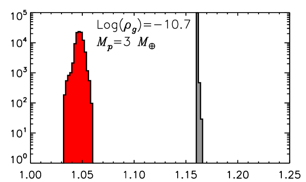
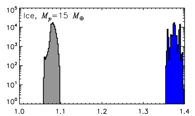
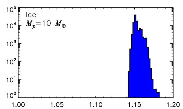
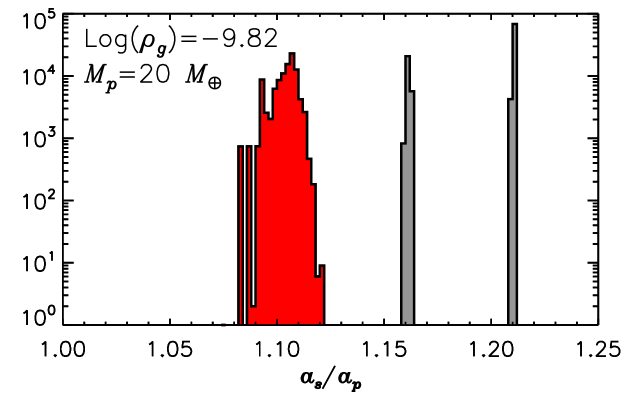
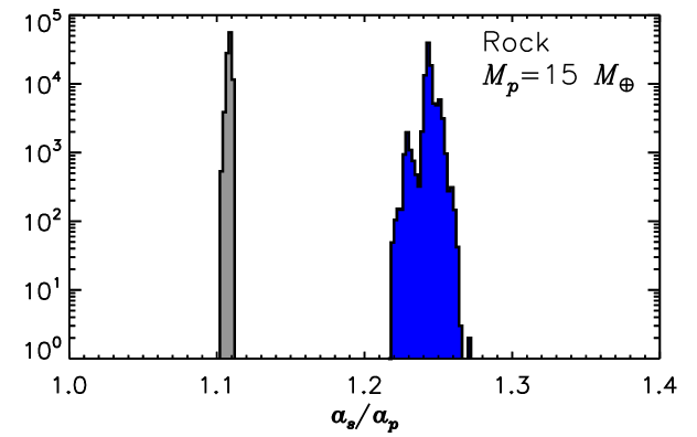
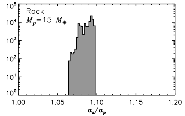
Figure 12: Semi-major axis distributions of segregated particles for models with $a_{p}=1$ (left), $5$ (center), and $10\,\mbox{au}$ (right). In the left panels, $\rho_{g}$ represents the unperturbed gas density at $r=a_{p}$, in units of $\mathrm{g\,cm}^{-3}$. Blue, red, and gray histograms refer to $R_{s}=1$, $100$, and $1000\,\mathrm{cm}$ particles, respectively. Segregation also occurs in other models not shown.

In the two cases shown in Figure 11 (icy and rocky particles), $K$ is large enough for gas drag to overcome the resonant forcing so that the simulated particles can drift inward, inside the planet’s orbit. Other models, however, do result in particles segregated in exterior orbits (over the course of the calculation). Some examples are illustrated in Figure 12. The trapped particles in the figure have orbits basically co-planar with the planet and their eccentricities are typically small, $e_{s}\lesssim H_{g}/a_{s}$. The semi-major axis distribution of the $10\,\mathrm{m}$ solids (gray histograms) can be very narrow, indicating segregation at locations of mean-motion resonances with the planet. Such are the cases shown in the left panels ($4:5$ and $3:4$ mean-motion resonances) and in the bottom-middle panel ($6:7$ mean-motion resonance), but other instances occur. The equilibrium eccentricities of solids trapped in mean-motion resonances are $\lesssim H_{g}/(2a_{s})$, in accord with the estimate of Weidenschilling & Davis (1985).

The minimum distance $\Delta r=r-a_{p}$ at which particles can be trapped at resonant locations depends on resonance overlap, which may lead to chaotic orbits (Wisdom, 1980). Duncan et al. (1989) found that a limit for resonance overlap is given by $|a_{s}-a_{p}|/a_{p}\approx 1.5(\mbox{$M_{p}$}/\mbox{$M_{\star}$})^{2/7}$, ranging from $\approx 0.06$ to $\approx 0.09$ for the cases illustrated in Figure 12. Kary et al. (1993) found an additional limit related to orbital energy dissipation by gas drag and estimated that orbital stability is possible as long as $|a_{s}-a_{p}|/a_{p}\gtrsim 1.6[(H_{g}/a_{p})(\mbox{$M_{p}$}/\mbox{$M_{\star}$})]^{2/9}$, whose value is comparable to Duncan et al.’s limit in the RHD calculations. The semi-major axis distributions of $10\,\mathrm{m}$ particles trapped in mean-motion resonances satisfy these theoretical limits.

The distributions of smaller particles in Figure 12 tend to be much broader, indicating that their segregation radii are associated to orbital locations where $\langle\Omega_{g}\rangle$ exceeds its unperturbed value. In the proximity but interior to these radii, drag torques tend to push solids outward. A planetary-mass body exerts a positive tidal torque on the exterior disk, transferring angular momentum and hence augmenting the gas rotation rate relative to that of an unperturbed disk. The torque density per unit disk mass is $\propto(\mbox{$M_{p}$}/\mbox{$M_{\star}$})^{2}(a_{p}/\Delta r)^{4}$ (Lin & Papaloizou, 1986) and peaks for $\Delta r\approx H_{g}$ when $\mbox{$R_{\mathrm{H}}$}\leq H_{g}$ (D’Angelo & Lubow, 2010). When integrated over the disk mass exterior to the planet, one finds the well-known result that the one-sided torque exerted by the planet is $\propto(\mbox{$M_{p}$}/\mbox{$M_{\star}$})^{2}(a_{p}/H_{g})^{3}$ (see, e.g., Lubow & Ida, 2010). Since the torque density function has a peak of finite width, particles well-coupled to the gas can attain minimum trapping distances $a_{s}-a_{p}\sim H_{g}$ (if $\mbox{$R_{\mathrm{H}}$}\leq H_{g}$). Angular momentum transfer beyond $|\Delta r|\approx 3H_{g}$ becomes more inefficient (D’Angelo & Lubow, 2010), even though tidal perturbations in the gas can extend farther (see Figure 9). Gas density perturbations become increasingly prominent as $M_{p}$ grows, eventually leading to gap formation, which begins when tidal torques exceed viscous torques, i.e., when $(\mbox{$M_{p}$}/\mbox{$M_{\star}$})^{2}\gtrsim 3\pi\alpha_{g}(H_{g}/a_{p})^{5}$. In the models presented herein only the $\mbox{$M_{p}$}=20\,\mbox{$M_{\oplus}$}$ cases at $1\,\mbox{au}$ (marginally) satisfy this condition in the two coldest disks (see Table 1).

The $10\,\mathrm{m}$ particles too can stop at equilibrium locations dictated by disk-planet tidal perturbations, as suggested by the broad distributions of $a_{s}$ in, e.g., the top-middle and bottom-right panels of Figure 12. In fact, the values of $K$ are comparable in these two cases, as is the width $\Delta r$ of the confinement region.

Segregation would prevent accretion, isolating the planet from the solids. Lambrechts et al. (2014) argued that isolation can be achieved when $\mbox{$M_{p}$}/\mbox{$M_{\oplus}$}\approx 20\,[H_{g}/(0.05a_{p})]^{3}$. Dipierro & Laibe (2017) found a comparable limit for $\tau_{s}\Omega_{\mathrm{K}}\sim 1$, while Bitsch et al. (2018) estimated a mass larger by $\approx 25$% for the conditions realized in the RHD calculations. In the models with $a_{p}=5$ and $10\,\mbox{au}$, these “isolation” masses ($\approx 30\,\mbox{$M_{\oplus}$}$ and $\approx 50\,\mbox{$M_{\oplus}$}$, respectively) would be much larger than the planet masses modeled herein. Indeed, in none of the models, $10$–$100\,\mathrm{cm}$ particles are trapped in exterior orbits. However, at $5$ and $10\,\mbox{au}$, $R_{s}=1\,\mathrm{cm}$ and $10\,\mathrm{m}$ particles can be segregated by smaller, $10\,\mbox{$M_{\oplus}$}$ planets (see Figure 12).

At $a_{p}=1\,\mbox{au}$, the proposed isolation limit would range from $\approx 8\,\mbox{$M_{\oplus}$}$ (coldest, least dense disk) to $\approx 22\,\mbox{$M_{\oplus}$}$ (warmest, most dense disk). At least two of the $20\,\mbox{$M_{\oplus}$}$ models should thus show segregation of solids. At the lowest density ($\rho_{g}=2.0\times 10^{-11}\,\mbox{$\mathrm{g\,cm}^{-3}$}$), $R_{s}=1\,\mathrm{cm}$ solids are efficiently accreted while $R_{s}\geq 10\,\mathrm{cm}$ are segregated. At the intermediate density ($\rho_{g}\approx 10^{-10}\,\mbox{$\mathrm{g\,cm}^{-3}$}$), $R_{s}\leq 10\,\mathrm{cm}$ particles are efficiently accreted, whereas larger ones are segregated. At the largest density, $1\,\mathrm{cm}$ and $10\,\mathrm{m}$ solids are segregated. Nonetheless, even $3\,\mbox{$M_{\oplus}$}$ planets can segregate solids under appropriate conditions, as shown in the top-left panel of Figure 12.

Continued accumulation of solids at segregation sites may enhance collisional comminution, possibly releasing some of the mass in the form of smaller particles, which may drift inward. Coagulation into larger bodies may also reactivate accretion of heavy elements on the planet.

3.4 Accretion Efficiencies

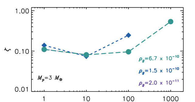
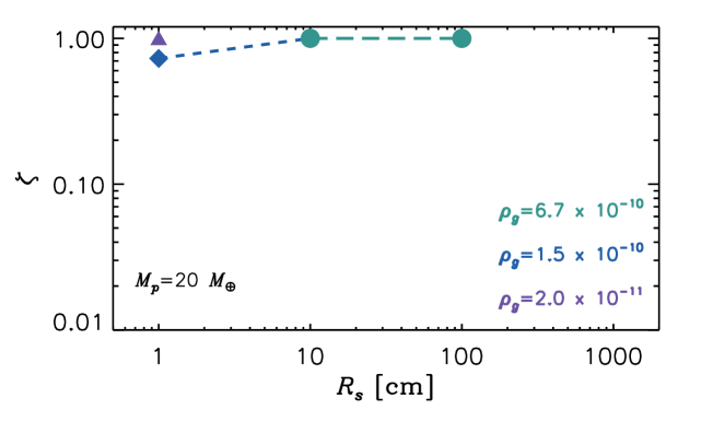
Figure 13: Accretion efficiencies versus particle radius, obtained from the RHD calculations at $a_{p}=1\,\mbox{au}$, for an $\mbox{$M_{p}$}=3$ (top) and $20\,\mbox{$M_{\oplus}$}$ planet (bottom). Different colors/symbols refer to different values of the reference gas density, as indicated (see also Table 1). Non-accreted solids are either segregated in exterior orbits or drift toward the star. Missing symbols indicate $\zeta=0$. In the top panel, efficiencies are comparable, at all three values of the gas density, for $R_{s}=1$ and $10\,\mathrm{cm}$ particles.

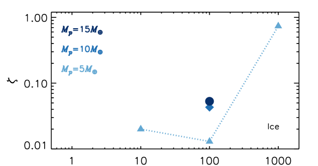
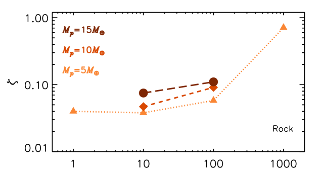
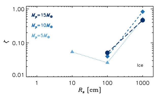
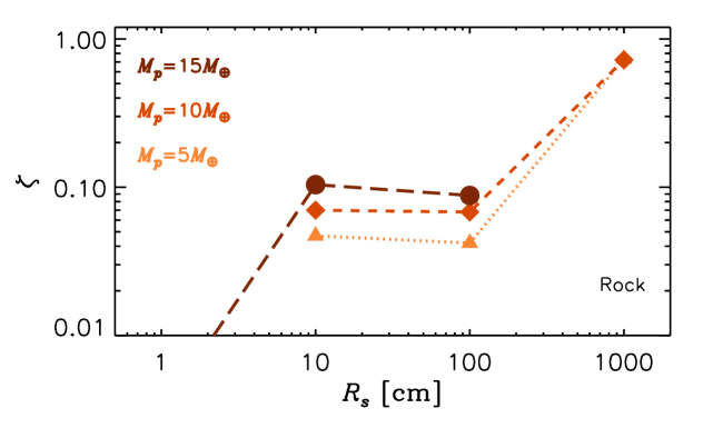
Figure 14: Accretion efficiencies obtained from the RHD calculations at $a_{p}=5$ (top) and $10\,\mbox{au}$ (bottom). Icy and rocky solids are represented on the left and right, respectively. Different colors/symbols refer to different planet masses, as indicated. Different line styles connect symbols of the same type and color. Missing symbols indicate $\zeta=0$. Non-accreted solids are segregated on exterior orbits or drift toward the inner disk. Icy particles can also evaporate.

The efficiency or probability of accretion, $\zeta$, in these models is computed as the ratio of the solids’ mass accreted by the planet to the solids’s mass interacting with the planet, as they drift inward. Interacting particles can be accreted, transferred to inner orbits, or segregated in the outer disk. Scattering out of the computational domain is possible but rare.

Icy particles can undergo ablation. In the models with $a_{p}=5\,\mbox{au}$, all particles drifting inward of $r\approx 4\,\mbox{au}$ ($T_{g}\approx 150\,\mbox{$\mathrm{K}$}$) are consumed to some extent. For a fixed particle temperature $T_{s}$, the ablation timescale is $\propto R_{s}$ (DP15). At $T_{s}\approx 150\,\mbox{$\mathrm{K}$}$, this time is in excess of $10^{4}$ years for $10\,\mathrm{m}$ solids, but much shorter for $\mathrm{cm}$-size particles. Since gas temperature in the proximity of a planet is higher than the average disk temperature at $r=a_{p}$ (DB13), particles can shed mass before being accreted. This process does indeed occur, typically reducing the accreted mass by $\lesssim 15$% at $a_{p}=5\,\mbox{au}$ and by $\lesssim 7$% at $a_{p}=10\,\mbox{au}$. The ablated mass is expected to increase in warmer disks and as $M_{p}$ increases.

The accretion efficiencies obtained from the RHD calculations are plotted in Figures 13 and 14. At $a_{p}=1\,\mbox{au}$, the $\mbox{$M_{p}$}=3\,\mbox{$M_{\oplus}$}$ planet typically accretes rocks with efficiencies $\lesssim 10$%, with few exceptions (Figure 13, top panel). The largest, $10\,\mathrm{m}$ particles can also be segregated, more often in the $\mbox{$M_{p}$}=20\,\mbox{$M_{\oplus}$}$ planet cases (see bottom panel). In these latter models, when particles accrete, they do so at high efficiency.

At $a_{p}=5$ and $10\,\mbox{au}$, there are some similarities among the models in terms of accretion efficiency (see Figure 14). Particles of $1\,\mathrm{cm}$ in radius are accreted inefficiently (a few percent or less). Missing symbols in the figure indicate zero efficiency, but not necessarily segregation in exterior orbits. Solids of $10$ and $100\,\mathrm{cm}$ in radius are generally accreted with $\zeta$ of a few to several percent, with peaks of $\approx 10$%. The $10\,\mathrm{m}$ particles are accreted efficiently, when accreted, with $0.5\lesssim\zeta\lesssim 0.8$. However, in a number of cases ($\mbox{$M_{p}$}\geq 10\,\mbox{$M_{\oplus}$}$), $10\,\mathrm{m}$ icy and rocky solids are segregated in the exterior disk (see also Figure 12).

Overall, the results in Figures 13 and 14 are in general accord with those from the simplified calculations shown in Figure 8. The values of $\zeta$ for $1$, $10$, and $100\,\mathrm{cm}$ solids are comparable. The typically large efficiency for the accretion of $10\,\mathrm{m}$ particles (when not segregated) is also in reasonable agreement.

Morbidelli & Nesvorny (2012) estimated small solid’s accretion on $\mbox{$M_{p}$}=1$ and $5\,\mbox{$M_{\oplus}$}$ planets with $a_{p}=0.8\,\mbox{au}$. They found efficiencies ranging from a few to several percent for $R_{s}\approx 10$–$100\,\mathrm{cm}$ particles. They also found that $10\,\mathrm{m}$ solids have much larger accretion efficiencies, in excess of $\approx 50$%. These predictions are generally consistent with those shown in Figures 13 and 14. Although they used an unperturbed surface density twice as large as the largest density applied in the RHD calculations (see Figure 9), the value of $\tau_{s}\Omega_{\mathrm{K}}$ for these particles was comparable, $\approx 0.1$–$100$.

Picogna et al. (2018) estimated particle accretion efficiencies from hydrodynamics calculations of laminar and turbulent disks. In models of $5$ and $10\,\mbox{$M_{\oplus}$}$ planets, they found $\zeta\approx 0.2$ at $\tau_{s}\Omega_{\mathrm{K}}\approx 0.01$ and $\approx 0.4$ at $\tau_{s}\Omega_{\mathrm{K}}\approx 100$, with a minimum around a few percent at $\tau_{s}\Omega_{\mathrm{K}}\sim 1$. Their results are similar to those presented in Figure 14 in the range $0.1\lesssim\tau_{s}\Omega_{\mathrm{K}}\lesssim 10$, although $\zeta$ is somewhat larger for $\approx 1\,\mathrm{cm}$ particles and somewhat smaller for $\approx 10\,\mathrm{m}$ particles than reported herein.

At an accretion rate of $\dot{M_{s}}\sim 10^{-5}\,\mathrm{\mbox{$M_{\oplus}$}\,yr^{-1}}$ (see Figure 5) and $\zeta\approx 0.1$, a $3\,\mbox{$M_{\oplus}$}$ planet at $1\,\mbox{au}$ would double its mass in $\sim 10^{6}\,\mathrm{yr}$, whereas a $20\,\mbox{$M_{\oplus}$}$ planet could grow by up to $1\,\mbox{$M_{\oplus}$}$ every $10^{5}\,\mathrm{yr}$ ($\zeta\approx 1$), if not isolated. At $5$ and $10\,\mbox{au}$, by accreting either icy or rocky $R_{s}\leq 100\,\mathrm{cm}$ solids, the accretion rate of a $5\,\mbox{$M_{\oplus}$}$ planet would be $\dot{M}_{p}\lesssim 10^{-6}\,\mathrm{\mbox{$M_{\oplus}$}\,yr^{-1}}$, but it could be many times as large if it accreted $10\,\mathrm{m}$ particles, resulting in a mass-doubling timescale of several times $10^{5}\,\mathrm{yr}$. More massive, $10$–$15\,\mbox{$M_{\oplus}$}$ planets would accrete at comparable rates, although the interaction with $10\,\mathrm{m}$ solids would typically lead to segregation rather than to accretion.

4 Accretion Efficiency of Bare Cores

Kary et al. (1993) found that the accretion efficiency is inversely proportional to the radial velocity of a particle, defined by Equation (22), in units of Hill radius per synodic period (at $\Delta r=2\sqrt{3}\mbox{$R_{\mathrm{H}}$}$), i.e.,

$$\zeta_{\mathrm{KLG}}\propto\frac{1}{K}\left(\frac{a_{p}}{H_{g}}\right)^{4}\left(\frac{\mbox{$R_{\mathrm{H}}$}}{a_{p}}\right)^{2},$$ (23)

hence $\zeta_{\mathrm{KLG}}\propto 1/K$ (see Equation (21)), for given planet and disk conditions, and proportional to $R_{s}/C_{D}$ for a given material. Their calculations and those presented in Sections 2.2 and 2.3 are most appropriate in the case of small tidal perturbations by the planet, i.e., when

$$\left(\frac{\mbox{$M_{p}$}}{\mbox{$M_{\star}$}}\right)^{2}<3\pi\alpha_{g}\left(\frac{H_{g}}{a_{p}}\right)^{5}.$$ (24)

If $\alpha_{g}\approx 10^{-3}$ and $H_{g}/a_{p}=0.022(a_{p}/\mbox{au})^{2/7}$, this limit would require $\mbox{$M_{p}$}/\mbox{$M_{\star}$}<2\times 10^{-5}$, or $\approx 6\,\mbox{$M_{\oplus}$}$ at $5\,\mbox{au}$ from a solar-mass star.

A set of calculations, similar to those discussed in Section 2.2, were performed to evaluate the accretion efficiency of $R_{s}=1$, $10$, $100$, and $1000\,\mathrm{cm}$ rocky/icy solids on small cores, $\mbox{$M_{p}$}\leq 1\,\mbox{$M_{\oplus}$}$, orbiting at $a_{p}=1$, $5$, and $10\,\mbox{au}$ from a $1\,\mbox{$M_{\odot}$}$ star. The nebula model is based on that of Chiang & Youdin (2010). The cores are “bare” in the sense that they do not bear a bound atmosphere, an appropriate approximation at such low masses (see, e.g., Kuwahara & Kurokawa, 2024). Therefore, these planets are assumed to be composed entirely of condensible materials and solids accrete when they hit the condensed surface of the planet. Although there is no local enhancement of the gas density close to the planet, gas drag operates all the way down to its surface, thus mimicking a low-density atmosphere.

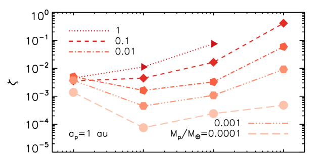
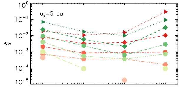
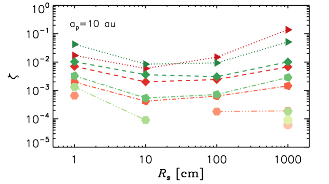
Figure 15: Accretion efficiencies of bare cores (i.e., without an atmosphere), versus particle radius, for rocky (red colors) and icy particles (green colors). The planet’s semi-major axis is $a_{p}=1$ (top), $5$ (center), and $10\,\mbox{au}$ (bottom) and the mass is indicated in the legend. The disk model is the same as that in Figure 4. Missing symbols indicate $\zeta=0$.

Results from these calculations are illustrated in Figure 15. The efficiency $\zeta$ is plotted as a function of $R_{s}$, for each core mass (see legend of the top panel). Missing symbols indicate that no collision was detected ($\zeta=0$). The largest particles tend to accrete more efficiently, although they can become trapped in exterior mean-motion resonances (see top panel, $\mbox{$M_{p}$}=1\,\mbox{$M_{\oplus}$}$ case). The mass scaling in Figure 15 agrees reasonably well with the predictions of Equations (14) and (23), $\zeta\propto M_{p}^{2/3}$, at $a_{p}=5$ and $10\,\mbox{au}$ ($\zeta/\mbox{$M_{p}$}^{2/3}$ varies by a factor $\lesssim 10$). At $a_{p}=1\,\mbox{au}$, this scaling is restricted to particles with $\tau_{s}\Omega_{\mathrm{K}}\gtrsim 0.1$.

5 Formation and Structure Models

The flow rate of $1$–$1000\,\mathrm{cm}$ solids through a disk, $\dot{M}_{s}=\dot{M}_{s}(t,R_{s})$, obtained from Equation (10) (see, e.g., Figure 5) and the efficiencies illustrated in Figure 13, 14, and 15 (appropriately interpolated in planet mass), $\zeta=\zeta(\mbox{$M_{p}$},R_{s})$, are combined to provide a size-integrated accretion rate,

$$\dot{M}_{Z}(\mbox{$M_{p}$},t)=\int\zeta(\mbox{$M_{p}$},R_{s})\,d\dot{M}_{s}(t,R_{s}),$$ (25)

to formation calculations at $1$, $5$, and $10\,\mbox{au}$. Accretion of rocks ($a_{p}=1$, $5\,\mbox{au}$) and ice ($a_{p}=5$, $10\,\mbox{au}$) is considered in separate models. The total mass of the disk is $\approx 0.055\,\mbox{$M_{\odot}$}$ at $t=0$. The initial gas-to-solids mass ratio is $100$ and $71.5$ (Pollack et al., 1994) in the rocky and icy disk, respectively. Formation starts from $\mbox{$M_{p}$}=10^{-2}\,\mbox{$M_{\oplus}$}$ embryos at $t=1000$ orbits (at each distance). Assuming mass equipartition among particle sizes, these embryos take $\approx 0.25$ to $\approx 0.55\,\mbox{Myr}$ to attain $\approx 1\,\mbox{$M_{\oplus}$}$, when structure calculations begin ($\dot{M}_{p}=\dot{M}_{Z}$ at smaller masses).

Planet evolution is modeled as in D’Angelo et al. (2014), by solving the structure equations in spherical symmetry (Kippenhahn et al., 2013), including mass and energy deposited by incoming solids and gas, particle break-up and ablation. Dust opacity in the envelope is computed self-consistently with sedimentation and coagulation of grains released by accreted gas and solids (Movshovitz et al., 2010). Dissolution and mixing of heavy elements in H-He gas (e.g., Bodenheimer et al., 2018) is neglected and all heavy elements settle to the condensed core. When the planet is in contact with the nebula, its radius $R_{p}$ is evaluated as in Lissauer et al. (2009), and depends on both the Bondi and Hill radius. Mass loss is enabled when the envelope overflows its boundary. Disk-limited accretion of gas is accounted for as in D’Angelo & Bodenheimer (2016). Disk evolution is modeled as outlined in Section 2.1 (see Figure 4). Formation continues until gas dispersal, at $t\approx 3.5\,\mbox{Myr}$.

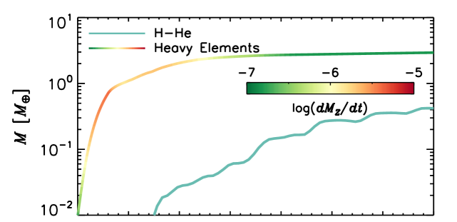
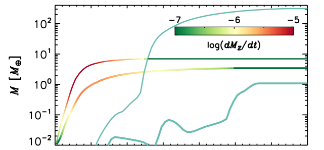
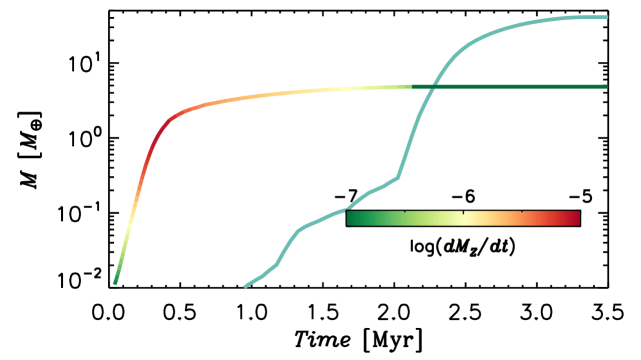
Figure 16: Heavy-element and H-He masses obtained from formation models at $a_{p}=1$ (top), $5$, and $10\,\mbox{au}$ (bottom). The heavy-element mass is color-coded by the solids’ accretion rate, in units of $\mbox{$M_{\oplus}$}\,\mathrm{yr}^{-1}$. Thinner lines in the middle panel refer to planets accreting icy particles.

The heavy-element and H-He masses of the planets are shown in Figure 16. Models at $1$ and $5\,\mbox{au}$ accreting silicates achieve masses $M_{Z}\approx 3$ and $3.4\,\mbox{$M_{\oplus}$}$, and H-He inventories contributing respectively $12$ and $24$% of the total masses. Instead, models accreting ice become gas giants, $\mbox{$M_{p}$}=321\,\mbox{$M_{\oplus}$}$ ($M_{Z}=6.9\,\mbox{$M_{\oplus}$}$) at $5\,\mbox{au}$ and $\mbox{$M_{p}$}=46\,\mbox{$M_{\oplus}$}$ ($M_{Z}=4.8\,\mbox{$M_{\oplus}$}$) at $10\,\mbox{au}$. For an initial gas-to-solids mass ratio equal to $100$, the heavy-element inventory at this latter distance would be limited to $\approx 1$ or $2.5\,\mbox{$M_{\oplus}$}$ by accreting rocks or ice, respectively.

The different outcomes at $5\,\mbox{au}$ can be attributed to the different amounts of solids transported across the planet’s orbit during formation: $\approx 150\,\mbox{$M_{\oplus}$}$ in the case of ice and $\approx 90\,\mbox{$M_{\oplus}$}$ in the case of rocks. Had the initial gas-to-solids mass ratio in the former case been $100$ (as in the rocky disk), this mass would have been $\approx 107\,\mbox{$M_{\oplus}$}$. The cumulative accretion efficiency, i.e., $M_{Z}$ divided by the amount of solids crossing the orbit of the planet, also contributes, with that of icy particles ($\approx 0.046$) exceeding by about $20$% that of rocky particles. In both models, most of the heavy-element mass ($\approx 70$%) is delivered by $10\,\mathrm{m}$ boulders/ice blocks. Only $10$–$15$% of $M_{Z}$ is supplied by $10$–$100\,\mathrm{cm}$ solids.

In the models at $1$ and $10\,\mbox{au}$, the total solid mass crossing the planet’s orbit is $\approx 103$ and $136\,\mbox{$M_{\oplus}$}$, respectively, corresponding to cumulative accretion efficiencies of $0.03$ and $0.04$. In these two calculations, about half of $M_{Z}$ is delivered by $100\,\mathrm{cm}$ boulders, at $1\,\mbox{au}$, and by $10\,\mathrm{m}$ ice blocks, at $10\,\mbox{au}$. Note that a $50/50$ solid mixture (by mass) of ice and silicates would have a material density closer to that of ice and, therefore, is expected to behave somewhat closer to ice than to silicates in terms of transport and accretion.

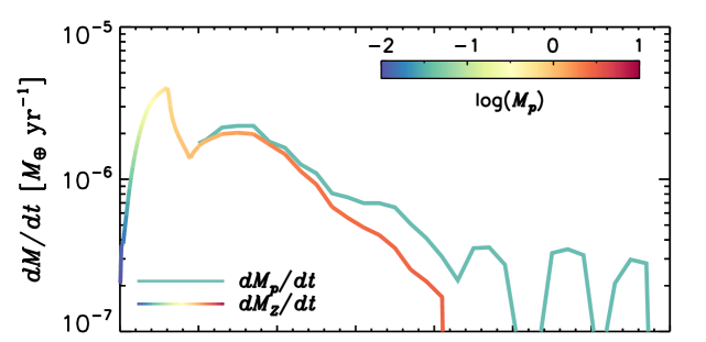
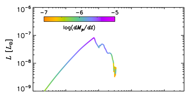
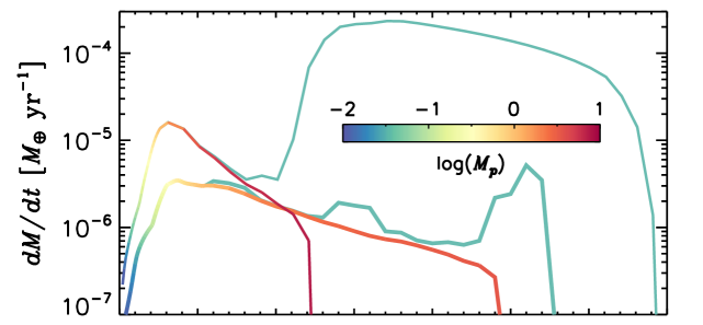
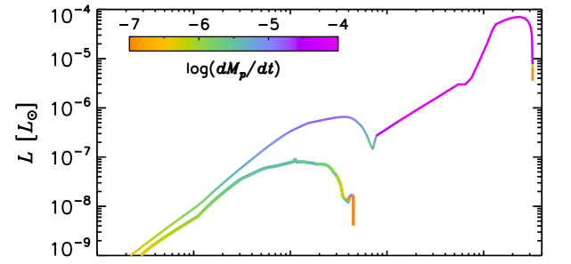
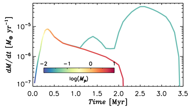
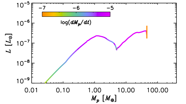
Figure 17: Accretion rates versus time (left) and luminosity versus mass (right) from formation models at $a_{p}=1$ (top), $5$, and $10\,\mbox{au}$ (bottom). The accretion rate of solids is color-coded by the planet mass (in units of $M_{\oplus}$) and the luminosity by total accretion rate (in units of $\mbox{$M_{\oplus}$}\,\mathrm{yr}^{-1}$). Thinner lines in the middle panels refer to planets accreting icy particles.

The H-He mass at the beginning of the structure calculations, $\approx 10^{-5}\,\mbox{$M_{\oplus}$}$, is negligible and remains so for $\sim 1\,\mbox{Myr}$ (see Figure 16). In fact, the total accretion rate $\dot{M}_{p}$ remains close to $\dot{M}_{Z}$ for a large part of the formation epoch (see left panels of Figure 17). The maximum of $\dot{M}_{Z}$ is achieved between $\mbox{$M_{p}$}=0.5$ and $1\,\mbox{$M_{\oplus}$}$ when heavy elements are supplied by silicates, and between $\mbox{$M_{p}$}=1$ and $2\,\mbox{$M_{\oplus}$}$ when they are supplied by ice. At $1\,\mbox{au}$, the accretion rate of gas exceeds $50$% that of solids only after $1.6\,\mathrm{Myr}$, when $\dot{M}_{Z}\lesssim 4\times 10^{-7}\,\mathrm{\mbox{$M_{\oplus}$}\,yr^{-1}}$. The planet accreting rocks at $5\,\mbox{au}$ first reaches this condition around $1.5\,\mathrm{Myr}$ ($\dot{M}_{Z}\approx 10^{-6}\,\mathrm{\mbox{$M_{\oplus}$}\,yr^{-1}}$, see middle panel), and then again when $\dot{M}_{Z}\lesssim 4\times 10^{-7}\,\mathrm{\mbox{$M_{\oplus}$}\,yr^{-1}}$. Mass loss by overflow is significant in this case during the first $\approx 2\,\mbox{Myr}$. During the formation of gas giants, the accretion rate of gas exceeds $\dot{M}_{Z}$ after $\approx 1\,\mathrm{Myr}$, when $M_{Z}$ has nearly attained its final value (see Figure 16).

Instead of mass equipartition, if all of the initial mass had been carried by particles of a single size, in general $M_{Z}$ would have been largest by accreting $R_{s}=1$–$10\,\mathrm{m}$ boulders/ice blocks. However, the final heavy-element inventory of a planet is not only determined by the mass distribution of particles but also by accretion of gas, since $\zeta$ is a function of $M_{p}$.

The luminosity during formation is shown in the right panels of Figure 17. Prior to beginning the structure calculations ($\mbox{$M_{p}$}\lesssim 1\,\mbox{$M_{\oplus}$}$), the luminosity is computed as $L=GM_{Z}\dot{M}_{Z}/\mbox{$R_{p}$}$, where $R_{p}$ is the radius of the condensed core. The curves are color-coded by the total accretion rate. The first luminosity peak corresponds to the maximum of $\dot{M}_{Z}$. For the gas giants, a second peak occurs around the maximum of the gas accretion rate. Although the planet accreting silicates at $5\,\mbox{au}$ exhibits a maximum in gas accretion around $2.6\,\mbox{Myr}$, the corresponding luminosity peak is smaller than the first because of the larger planet radius. In fact, both lower-mass planets remain in contact with the disk until it completely disperses. Therefore, their envelopes remain extended throughout formation. The gas giants, instead, detach from the disk when $t\approx 1.2$ and $2.2\,\mbox{Myr}$ at $5$ and $10\,\mbox{au}$, respectively. They undergo disk-limited accretion thereafter.

Dissolution of heavy elements in the interior of the planets may produce a stratification in composition and possibly affect energy transport and temperatures (e.g., Bodenheimer et al., 2018; Stevenson et al., 2022). Although heavy-element deposition resulting from accretion of small solids can differ from that resulting from planetesimal accretion, the radial composition of an interior may not provide distinctive information on the original carriers after sustained mixing. Moreover, the deposition of refractory material may not differentiate between accretion of small and large solids, as deposition patterns can overlap (see Appendix B).

6 Discussion and Conclusions

Accretion of small solids ($10^{-2}\lesssim\tau_{s}\Omega_{\mathrm{K}}\lesssim 10^{2}$) on a planet depends on the transport of solids through the disk, $dM_{s}/dt$, and on the efficiency of accretion, $\zeta$ (see Equation (25)). The former quantity is non-local, and determined by the global evolution of disk’s gas, the initial distribution of solids, coagulation and fragmentation. The latter quantity (i.e., the fraction of $dM_{s}/dt$ at $a_{p}$ that is accreted by the planet) is determined by multiple processes, at orbital or smaller scales. Small cores without an envelope allow for relatively straightforward calculations of $\zeta$, including planet-induced velocity perturbations on the gas (see Section 4). However, as the planet grows larger, the computation of $\zeta$ becomes increasingly complex. In fact, tidal interactions between the planet and the disk have important effects on solids dynamics. Close-range, 3D gas thermodynamics is also expected to significantly affect $\zeta$. Tidal segregation (and capture in mean-motion resonances) can impede the flux of solids through the planet’s orbit, a process that depends on solid size and composition, planet mass, and on the gas thermal state (and, therefore, on disk age and mass). The epoch of accretion is also limited by the duration of solids’ transport across the planet forming region. Boulder-size solids tend to accrete more efficiently than smaller solids, unless they become segregated. A disk of initial mass $0.055\,\mbox{$M_{\odot}$}$ in gas and $\approx 260\mbox{$M_{\oplus}$}$ in solids would provide typical accretion rates of heavy elements (in the $1$–$10\,\mbox{au}$ region) between $10^{-6}$ and $10^{-5}\,\mathrm{\mbox{$M_{\oplus}$}\,yr^{-1}}$, for the first $1$–$1.5\,\mbox{Myr}$ of evolution, and $\lesssim 10^{-6}\,\mathrm{\mbox{$M_{\oplus}$}\,yr^{-1}}$ thereafter (see Figure 17).

The results presented in Figures 4 and 5 are specific to the applied (global) disk conditions but appropriate solutions can be found by integrating Equations  9 and 10 in relevant gaseous disks. The efficiencies of accretion presented in Figures 13 and 14 are more general, since they only depend on local quantities, and can be used as long as gas densities and temperatures are comparable to those assumed in the RHD calculations (see Table 1). The same considerations apply to the efficiencies of small cores with no envelope reported in Figure 15.

The formation calculations presented herein apply accretion rates of solids based on simple, but consistent, models of gas and solids disk evolution and first-principle determinations of accretion efficiencies. Structure calculations include detailed computations of grain opacity as solids travel through the envelope and release material. Outcomes encompass a broad range, from low-mass, heavy-element dominated planets to H-He gas giants. Heavy-element masses from $3$ to $7\,\mbox{$M_{\oplus}$}$ require an amount of solids from $\approx 90$ to $150\,\mbox{$M_{\oplus}$}$ to cross the planet’s orbit. The maximum luminosity emitted during the epoch of solids’ accretion ranges from $\approx 10^{-7}$ to $\approx 10^{-6}\,L_{\odot}$.

Cumulative efficiencies of accretion in the formation calculations are below $5$%. Multiple planets may form if solids can drift inward, past a planet. Heavy elements would be delivered during the epoch when $d{M}_{s}/dt$ at a given distance is non-negligible. As outer planets remove solids, lesser amounts would be available to inner planets. Higher efficiency of accretion in a size range implies lower availability to planets downstream. Because of segregation, a planet large enough (a few to several times $M_{\oplus}$, see Figure 12) could hinder or terminate the supply of solid (in some size range) to inner planets. In summary, predictions on heavy-element delivery (to one or more planets) require accounting for both local and remote processes, over the disk lifetime. Considerations on the evolving size distribution of solids are also necessary, including at segregation sites, where enhanced comminution and/or growth may release solids and promote further accretion.

Appendix A Evolution of Solids in Quasi-Steady State Gas Fields

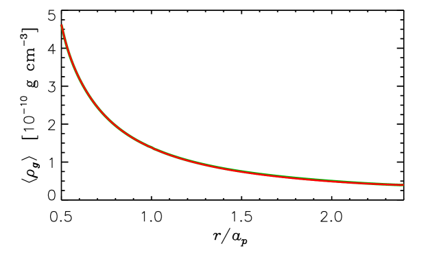
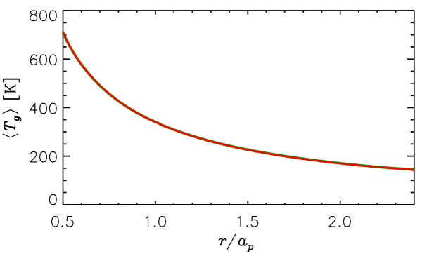
Figure 18: Azimuthal averages (around the star) versus radial distance of the mid-plane gas density (left) and mid-plane gas temperature (right) at the quasi-steady state $\mathcal{S}_{i}$ (green) and at the end of the test calculation (red), several hundred planet’s orbits later. Curves at the two epochs overlap one another in both panels (for better visibility, green curves are thicker than red curves).

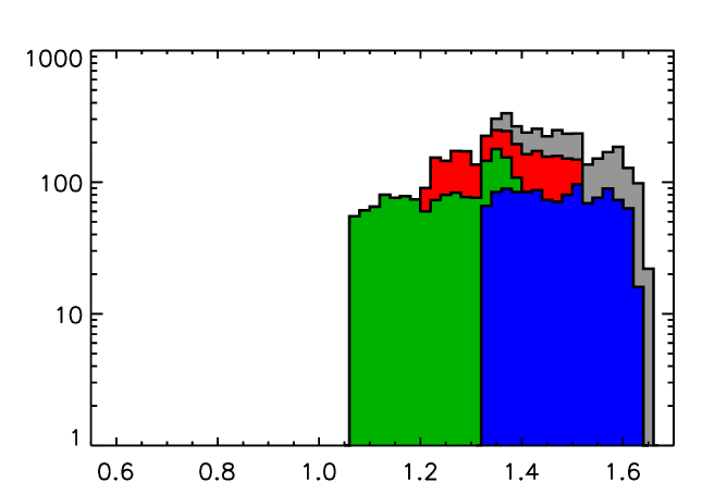
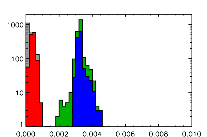
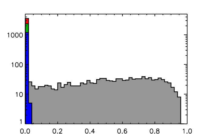
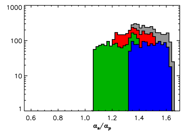
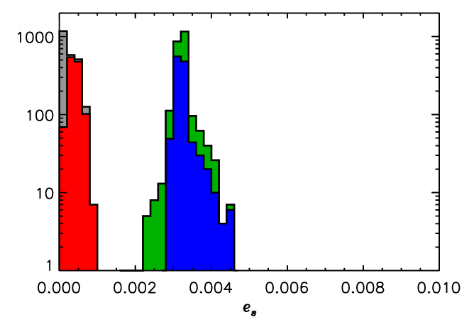
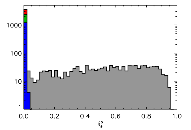
Figure 19: Histograms of the particles’ semi-major axes (left), eccentricities (center) and inclinations (right) as they approach the planet’s orbit. The top panel refers to the model in which the evolution of both the gas and the solids is calculated. In the bottom panel, the gas quasi-steady state $\mathcal{S}_{i}$ (defined in the text) is applied. The gray histograms include all particles; the red, green, and blue histograms include particles with radii $R_{s}\leq 100\,\mathrm{cm}$, $R_{s}\leq 10\,\mathrm{cm}$, and $R_{s}=1\,\mathrm{cm}$, respectively.

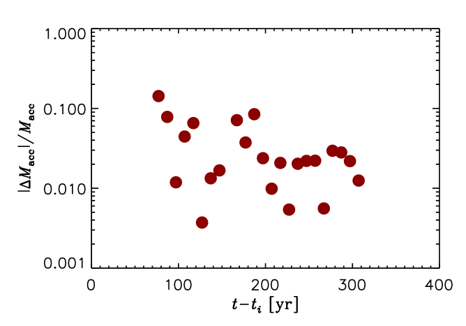
Figure 20: Normalized relative difference in the accretion rate of solids on the planet versus time, since the reference time of state $\mathcal{S}_{i}$ (defined in the text), between the two calculations described in the text. Accretion first involves $R_{s}=10\,\mathrm{cm}$ and then $R_{s}=100\,\mathrm{cm}$ particles.

The results of the RHD calculations presented in Section 3 rely on the assumption that the evolution of the disk’s gas can be neglected while the solids evolve through the gas. The assumption is justified by the fact that the gas fields $(\boldsymbol{u}_{g},\rho_{g},T_{g})$ are in a near-steady state in the frame co-rotating with the planet and do not change significantly over the course of the calculations. The approach is intended to mitigate the computational requirements of those RHD models and render the problem more tractable. Here a test is presented on the validation of this approach.

An RHD calculation of a $3\,\mbox{$M_{\oplus}$}$ planet, embedded in a disk at $r=a_{p}=1\,\mbox{au}$ from a $1\,\mbox{$M_{\odot}$}$ star, is performed and evolved until the system attains a state of quasi-equilibrium, hereafter referred to as state $\mathcal{S}_{i}$. The setup of the model is equivalent to that of the models with $a_{p}=1\,\mbox{au}$ discussed in Section 3 (reference density $\langle\rho_{g}\rangle=1.5\times 10^{-10}\,\mbox{$\mathrm{g\,cm}^{-3}$}$), but at a somewhat lower grid resolution. The planet radius is assumed to be approximately equal to $R_{\mathrm{B}}$. Four size bins, $R_{s}=1$, $10$, $100$, and $1000\,\mathrm{cm}$, are populated with equal numbers of rocky particles. They are deployed outside the planet’s orbit by applying the same random process as described in Section 3.3. The calculation is then continued, from state $\mathcal{S}_{i}$, by evolving both the gas and the solids for several hundred orbits of the planet. During this time, the disk’s gas density and temperature (red curves) do not deviate significantly from those of state $\mathcal{S}_{i}$ (green curves), as illustrated in Figure 18 (in which curves basically overlap). In another calculation, the same distribution of solids evolves in the gas fields provided by state $\mathcal{S}_{i}$.

The stopping times of the solids at deployment range from $\tau_{s}\Omega_{\mathrm{K}}\approx 10^{-2}$ ($R_{s}=1\,\mathrm{cm}$) to $\tau_{s}\Omega_{\mathrm{K}}\approx 10^{3}$ ($R_{s}=1000\,\mathrm{cm}$). Intermediate size particles ($0.1\lesssim\tau_{s}\Omega_{\mathrm{K}}\lesssim 10$) drift toward the planet relatively quickly. For solids in the various size ranges, Figure 19 shows the histograms of the particles’ semi-major axes (left), orbital eccentricities (center), and inclinations (right) during the approaching phase (see figure’s caption for further details). The orbits remain nearly circular, although the smallest particles are somewhat more eccentric than the largest ones (see also Figure 11). The inclination with respect to the mid-plane is basically zero, except for that of the largest particles, which is damped over a longer timescale ($\propto R_{s}$, Adachi et al., 1976). In statistical terms, the orbital elements of the solids in the two calculations remain quantitatively similar. By the end of the simulations, the $R_{s}=10$ and $100\,\mathrm{cm}$ particles have either accreted on the planet or moved toward interior orbits, whereas the smallest and largest particles continue drifting toward the planet.

In order to gauge variations in the accretion rates of solids on the planet, Figure 19 shows the relative difference of the accreted mass versus time, since state $\mathcal{S}_{i}$, between the two calculations. The $R_{s}=10\,\mathrm{cm}$ particles intercept the planet’s orbit first, followed by the $R_{s}=100\,\mathrm{cm}$ particles. The differences in accreted mass are below $\approx 10$%, and typically at the level of a few percent on average. The accretion efficiencies $\zeta$ are also in close agreement, within $\approx 1$%. The fact that the accretion rates of the particles are statistically consistent during close encounters with the planet implies that particle dynamics is indeed similar in the two simulated scenarios, even during the phases of the evolution preceding accretion.

Appendix B Dissolution of Solids in Planetary Envelopes

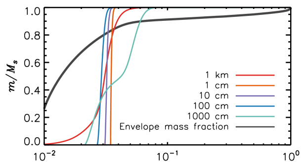
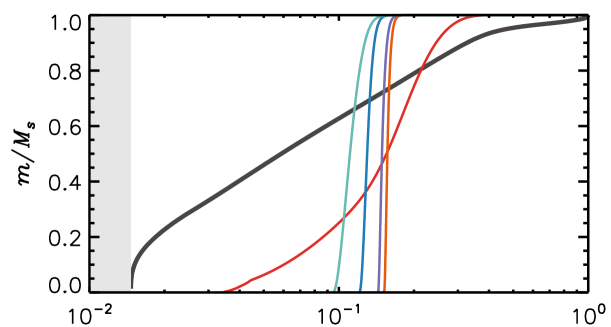
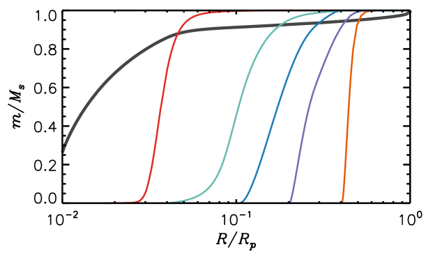
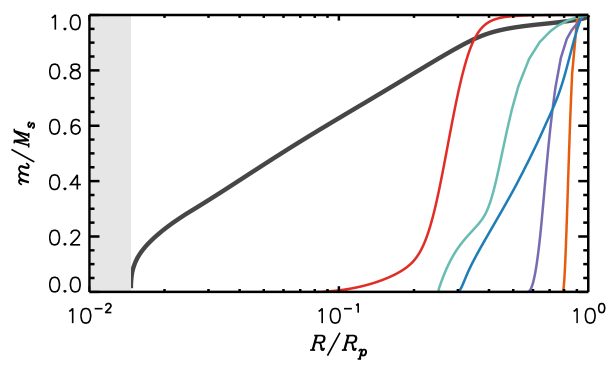
Figure 21: Mass evolution of rocky (SiO₂, top) and icy solids (bottom), versus planet radius, as they ablate while descending in a low-mass ($0.15\,\mbox{$M_{\oplus}$}$, left) and high-mass envelope ($6.9\,\mbox{$M_{\oplus}$}$, right). Interior structures are taken from the giant planet model at $5\,\mbox{au}$, discussed in Section 5. Solids have different initial sizes, as indicated in the legend of the top-left panel. Quantity $M_{s}$ refers to the initial mass entering the envelope. The thick gray lines indicate the envelope mass fraction. The shaded area in the right panels represents the condensed core region. See text for further details.

Solid bodies moving through an atmosphere warm up and ablate, disseminating heavy elements along their path. This process can affect the composition of planetary interiors. We performed experiments of solids’ dissolution in planetary envelopes taken from the giant planet formed at $5\,\mbox{au}$ and presented in Section 5. The envelopes refer to times at which their masses are $0.15\,\mbox{$M_{\oplus}$}$ ($\mbox{$M_{p}$}=6.8\,\mbox{$M_{\oplus}$}$) and $6.9\,\mbox{$M_{\oplus}$}$ ($\mbox{$M_{p}$}=13.8\,\mbox{$M_{\oplus}$}$). To circumvent segregation issues, solids were deployed around the planet’s $L_{2}$ point (or close enough to allow for accretion). The spread of the results due to possible differences in entry velocities was not assessed. Outside of the envelope, the disk is modeled as in the planet structure calculation (see Section 5).

The energy budget of a particle includes heating by frictional work and by the ambient thermal field of the envelope, and cooling by black-body radiation at the surface temperature and by latent heat release through phase change. Above the critical temperature of the material, all energy input drives mass loss (see DP15, for details). A body can break-up when subjected to a dynamical pressure larger than the compressive strength of the material, although break-up did not occur in these experiments.

The heavy-element deposition profiles of the rocky (SiO₂, top) and icy solids (H₂O, bottom) are illustrated in Figure 21. The high-mass envelope planet is shown on the right (shaded areas represent the condensed core region). Upon entry in the envelope, and prior to significant phase change, the surface temperature of $R_{s}\lesssim 10\,\mathrm{cm}$ particles tends to attain values similar to gas temperatures. In these cases, significant ablation begins only after envelope temperatures rise above some value, dictated by the vapor pressure curve of the material. When frictional heating exceeds warming by the local thermal field, deposition may begin at lower envelope temperatures. In the top panels of Figure 21, because of the contribution of frictional heating, $1\,\mathrm{km}$ planetesimals can disseminate heavy elements over a broad range of depths, including layers in which small solids would ablate. At all sizes, about $50$% of the input silicate mass would be released in the outer $15$–$20\%$ (top-left) and outer $25$–$35$% (top-right) of the envelope mass. Small icy solids (bottom panels) would be disseminated further up in the planet, compared to $1\,\mathrm{km}$ planetesimals. Nonetheless, for all sizes shown in the figure, $50\%$ of the accreted ice mass would be dispersed in the outer $5$–$15$% of the envelope mass. Thus, in all cases shown in Figure 21, most of the accreted solids would not settle to the core, as assumed in Section 5, but would result in an envelope enriched in heavy elements.

References

- Adachi et al. (1976) Adachi, I., Hayashi, C., & Nakazawa, K. 1976, Progress of Theoretical Physics, 56, 1756
- Andrews (2020) Andrews, S. M. 2020, ARA&A, 58, 483, doi: 10.1146/annurev-astro-031220-010302
- Bailey et al. (2023) Bailey, A., Stone, J., & Fung, J. 2023, arXiv e-prints, arXiv:2310.03116, doi: 10.48550/arXiv.2310.03116
- Bitsch et al. (2018) Bitsch, B., Morbidelli, A., Johansen, A., et al. 2018, A&A, 612, A30, doi: 10.1051/0004-6361/201731931
- Bodenheimer et al. (2018) Bodenheimer, P., Stevenson, D. J., Lissauer, J. J., & D’Angelo, G. 2018, ApJ, 868, 138, doi: 10.3847/1538-4357/aae928
- Boss & Myhill (1992) Boss, A. P., & Myhill, E. A. 1992, ApJS, 83, 311, doi: 10.1086/191739
- Bourdelle de Micas et al. (2022) Bourdelle de Micas, J., Fornasier, S., Avdellidou, C., et al. 2022, A&A, 665, A83, doi: 10.1051/0004-6361/202244099
- Castor (2007) Castor, J. I. 2007, Radiation Hydrodynamics (Cambridge, UK: Cambridge University Press)
- Chiang & Youdin (2010) Chiang, E., & Youdin, A. N. 2010, Annual Review of Earth and Planetary Sciences, 38, 493, doi: 10.1146/annurev-earth-040809-152513
- D’Alessio et al. (2001) D’Alessio, P., Calvet, N., & Hartmann, L. 2001, ApJ, 553, 321, doi: 10.1086/320655
- D’Alessio et al. (1998) D’Alessio, P., Canto, J., Calvet, N., & Lizano, S. 1998, ApJ, 500, 411, doi: 10.1086/305702
- D’Angelo & Bodenheimer (2013) D’Angelo, G., & Bodenheimer, P. 2013, ApJ, 778, 77, doi: 10.1088/0004-637X/778/1/77
- D’Angelo & Bodenheimer (2016) —. 2016, ApJ, 828, 33, doi: 10.3847/0004-637X/828/1/33
- D’Angelo & Lubow (2010) D’Angelo, G., & Lubow, S. H. 2010, ApJ, 724, 730, doi: 10.1088/0004-637X/724/1/730
- D’Angelo & Podolak (2015) D’Angelo, G., & Podolak, M. 2015, ApJ, 806, 203, doi: 10.1088/0004-637X/806/2/203
- D’Angelo et al. (2014) D’Angelo, G., Weidenschilling, S. J., Lissauer, J. J., & Bodenheimer, P. 2014, Icarus, 241, 298, doi: 10.1016/j.icarus.2014.06.029
- Dipierro & Laibe (2017) Dipierro, G., & Laibe, G. 2017, MNRAS, 469, 1932, doi: 10.1093/mnras/stx977
- Drazkowska et al. (2023) Drazkowska, J., Bitsch, B., Lambrechts, M., et al. 2023, in Astronomical Society of the Pacific Conference Series, Vol. 534, Protostars and Planets VII, ed. S. Inutsuka, Y. Aikawa, T. Muto, K. Tomida, & M. Tamura, 717, doi: 10.48550/arXiv.2203.09759
- Dubrulle et al. (1995) Dubrulle, B., Morfill, G., & Sterzik, M. 1995, Icarus, 114, 237, doi: 10.1006/icar.1995.1058
- Duncan et al. (1989) Duncan, M., Quinn, T., & Tremaine, S. 1989, Icarus, 82, 402, doi: 10.1016/0019-1035(89)90047-X
- Eggleton (1983) Eggleton, P. P. 1983, ApJ, 268, 368, doi: 10.1086/160960
- Ercolano & Pascucci (2017) Ercolano, B., & Pascucci, I. 2017, Royal Society Open Science, 4, 170114, doi: 10.1098/rsos.170114
- Flaherty et al. (2018) Flaherty, K. M., Hughes, A. M., Teague, R., et al. 2018, ApJ, 856, 117, doi: 10.3847/1538-4357/aab615
- Gary et al. (1972) Gary, M., McAfee, R. J., & Wolf, C. L. 1972, Glossary of Geology (Washington, D.C.: American Geological Institute)
- Gorti et al. (2009) Gorti, U., Dullemond, C. P., & Hollenbach, D. 2009, ApJ, 705, 1237, doi: 10.1088/0004-637X/705/2/1237
- Inaba & Ikoma (2003) Inaba, S., & Ikoma, M. 2003, A&A, 410, 711, doi: 10.1051/0004-6361:20031248
- Johansen & Lambrechts (2017) Johansen, A., & Lambrechts, M. 2017, Annual Review of Earth and Planetary Sciences, 45, 359, doi: 10.1146/annurev-earth-063016-020226
- Kary et al. (1993) Kary, D. M., Lissauer, J. J., & Greenzweig, Y. 1993, Icarus, 106, 288, doi: 10.1006/icar.1993.1172
- Kessler & Alibert (2023) Kessler, A., & Alibert, Y. 2023, A&A, 674, A144, doi: 10.1051/0004-6361/202245641
- Kippenhahn et al. (2013) Kippenhahn, R., Weigert, A., & Weiss, A. 2013, Stellar Structure and Evolution (Stellar Structure and Evolution: Astronomy and Astrophysics Library, ISBN 978-3-642-30255-8. Springer-Verlag Berlin Heidelberg, 2013), doi: 10.1007/978-3-642-30304-3
- Kuwahara & Kurokawa (2024) Kuwahara, A., & Kurokawa, H. 2024, A&A, 682, A14, doi: 10.1051/0004-6361/202347530
- Lambrechts & Johansen (2012) Lambrechts, M., & Johansen, A. 2012, A&A, 544, A32, doi: 10.1051/0004-6361/201219127
- Lambrechts et al. (2014) Lambrechts, M., Johansen, A., & Morbidelli, A. 2014, A&A, 572, A35, doi: 10.1051/0004-6361/201423814
- Levermore & Pomraning (1981) Levermore, C. D., & Pomraning, G. C. 1981, ApJ, 248, 321, doi: 10.1086/159157
- Lin & Papaloizou (1986) Lin, D. N. C., & Papaloizou, J. 1986, ApJ, 309, 846, doi: 10.1086/164653
- Lissauer (1987) Lissauer, J. J. 1987, Icarus, 69, 249, doi: 10.1016/0019-1035(87)90104-7
- Lissauer (1993) —. 1993, ARA&A, 31, 129, doi: 10.1146/annurev.aa.31.090193.001021
- Lissauer et al. (2009) Lissauer, J. J., Hubickyj, O., D’Angelo, G., & Bodenheimer, P. 2009, Icarus, 199, 338, doi: 10.1016/j.icarus.2008.10.004
- Lubow & Ida (2010) Lubow, S. H., & Ida, S. 2010, Planet Migration, ed. S. Seager (Exoplanets, edited by S. Seager. Tucson, AZ: University of Arizona Press), 347–371
- Lynden-Bell & Pringle (1974) Lynden-Bell, D., & Pringle, J. E. 1974, MNRAS, 168, 603, doi: 10.1093/mnras/168.3.603
- Melosh (2007) Melosh, H. J. 2007, Meteoritics & Planetary Science, 42, 2079, doi: 10.1111/j.1945-5100.2007.tb01009.x