Numerical validation of scaling laws for stratified turbulence

Abstract

Recent theoretical progress using multiscale asymptotic analysis has revealed various possible regimes of stratified turbulence. Notably, buoyancy transport can either be dominated by advection or diffusion, depending on the effective Péclet number of the flow. Two types of asymptotic models have been proposed, which yield measurably different predictions for the characteristic vertical velocity and length scale of the turbulent eddies in both diffusive and non-diffusive regimes. The first, termed a ‘single-scale model’, is designed to describe flow structures having large horizontal and small vertical scales, while the second, termed a ‘multiscale model’, additionally incorporates flow features with small horizontal scales, and reduces to the single-scale model in their absence. By comparing predicted vertical velocity scaling laws with direct numerical simulation data, we show that the multiscale model correctly captures the properties of strongly stratified turbulence within spatiotemporally-intermittent turbulent patches. Meanwhile its single-scale reduction accurately describes the more orderly layer-like flow outside those patches.

1 Introduction

Owing to the associated enhanced rates of irreversible scalar mixing, stratified turbulence is a critical process in the Earth’s atmosphere and oceans, impacting both weather and climate, and in the interiors of stars and gaseous planets, affecting their long-term evolution. Assuming that the buoyancy of the fluid is controlled by a single scalar field, which could be temperature or the concentration of a single solute, the dimensionless Boussinesq equations governing the fluid motions are

$$\frac{\partial\boldsymbol{u}}{\partial t}+\boldsymbol{u}\cdot\boldsymbol{\nabla}\boldsymbol{u} =-\nabla p+\frac{b}{Fr^{2}}\boldsymbol{e}_{z}+\frac{1}{Re}\nabla^{2}\boldsymbol{u}+\boldsymbol{F}_{h},$$ (1a)

$$\frac{\partial b}{\partial t}+\boldsymbol{u}\cdot\boldsymbol{\nabla}b+w =\frac{1}{Pe}\nabla^{2}b,$$ (1b)

$$\boldsymbol{\nabla}\cdot\boldsymbol{u} =0,$$ (1c)

where $\boldsymbol{u}=(u,v,w)$ is the velocity field expressed in units of $U$ (where $U$ is a characteristic horizontal velocity of the large-scale flow), $t$ is the time variable in units of $L/U$ (where $L$ is a characteristic large horizontal scale of the flow), $p$ is the pressure fluctuation away from hydrostatic equilibrium in units of $\rho_{m}U^{2}$ (where $\rho_{m}$ is the mean density of the fluid), and $b$ is the deviation of the buoyancy field away from a linearly stratified background, expressed in units of $LN^{2}$ (where $N$ is the buoyancy frequency of the stable stratification). The flow is assumed to be driven by a non-dimensional divergence-free horizontal force ${\boldsymbol{F}}_{h}$, which only varies on large spatial scales and long time scales. The unit vector $\boldsymbol{e}_{z}$ points in the direction opposite to gravity.

The usual dimensionless governing parameters of the flow emerge; namely, the Reynolds number $Re=UL/\nu$, the Péclet number $Pe=UL/\kappa$ and the Froude number $Fr=U/NL$, where $\nu$ is the kinematic viscosity, and $\kappa$ is the buoyancy diffusivity, while the Prandtl number, $Pr=\nu/\kappa=Pe/Re$ is a property of the fluid. Typically, $Pr\sim O(1)$ in air and water, but is very small in astrophysical fluids (of order $10^{-2}$ in degenerate plasmas and liquid metals, and much smaller in non-degenerate stellar plasmas, see Lignières,, 2020).

As the stratification increases ($Fr\rightarrow 0$), vertical motions are increasingly suppressed and restricted to small characteristic vertical scales $l_{z}=O(\alpha L)$, where the emergent aspect-ratio $\alpha$ is an increasing function of $Fr$ but could also depend on $Re$ and $Pe$. In the limit $(\alpha,Fr)\rightarrow 0$, asymptotic analysis has successfully been used to derive reduced equations for stratified turbulence and to gain insight into its properties. Brethouwer et al., (2007), following Billant and Chomaz, (2001), proposed an asymptotic reduction in which the vertical coordinate $z$ is rescaled as $\zeta=z/\alpha$ (with $\alpha\ll 1$), while the horizontal coordinates ${\boldsymbol{x}}_{h}=(x,y)$ remain of order unity. Accordingly, all dependent variables $q$ are expressed as $q({\boldsymbol{x}}_{h},\zeta,t;\alpha)$. As in Klein, (2010), we refer to this type of model, which is designed to capture the essence of a scale-specific process, as a single-scale asymptotic (SSA) model. This vertical rescaling, when used in (1), reveals the importance of the emergent buoyancy Reynolds and Péclet numbers, defined as

$$Re_{b}=\alpha^{2}Re\quad\mbox{ and }\quad Pe_{b}=\alpha^{2}Pe,$$ (2)

respectively. Brethouwer et al., (2007) showed that balancing the mass continuity equation in the limit $\alpha\rightarrow 0$ requires $w=O(\alpha)$. When $Re_{b}$ and $Pe_{b}$ are at least $O(1)$, dominant balance in the buoyancy equation implies $b=O(\alpha)$. Finally, the vertical component of the momentum equation reduces to hydrostatic equilibrium when $\alpha\rightarrow 0$, yielding $\alpha=Fr$, as first argued in the inviscid and non-diffusive case by Billant and Chomaz, (2001).

More recently, Shah et al., (2024) noted that in the limit of $Pr\ll 1$, it is possible to have a regime in which $Pe_{b}\ll 1\leq Re_{b}$. They demonstrated that in this case, the SSA model and corresponding asymptotic expansion reveal instead that $w=O(\alpha)$ and $b=O(\alpha Pe_{b})$, with $\alpha=(Fr^{2}/Pe)^{1/4}$ (see also Lignières,, 2020; Skoutnev,, 2023).

Crucial to the SSA theory is the notion that every component of the flow is strongly anisotropic, with large horizontal scales and a small vertical scale. In this model, therefore, the vertical fluid motions are primarily driven by the divergence of the horizontal flow, as illustrated schematically in figure 1. Chini et al., (2022), however, noted that the SSA theory ignores the possibility that isotropic motions with small horizontal scales may also exist and, in fact, are commonly seen in numerical simulations of stratified turbulence at sufficiently large $Re_{b}$ (cf. Maffioli and Davidson,, 2016; Cope et al.,, 2020; Garaud,, 2020). They proposed a new asymptotic reduction that explicitly incorporates two horizontal scales and two time scales, such that all dependent variables are expressed as

$$q({\boldsymbol{x}}_{f},\,{\boldsymbol{x}}_{s},\,\zeta,t_{f},t_{s};\alpha),\,\mbox{ }\mbox{where }{\boldsymbol{x}}_{s}={\boldsymbol{x}},\,{\boldsymbol{x}}_{f}={\boldsymbol{x}}/\alpha,\,t_{s}=t,\,t_{f}=t/\alpha,$$ (3)

and where the subscripts $s$ and $f$ are used to denote slow and fast scales, respectively. Again following Klein, (2010), we refer to the resulting reduced equations as a multiscale asymptotic (MSA) model. Chini et al., (2022) showed that these definitions imply that the large-scale motions remain strongly anisotropic with an aspect ratio $\alpha$, as in the SSA model, but can coexist with isotropic small-scale motions that evolve on the fast time scale $t_{f}$, and vary on the small vertical coordinate $\zeta$ and the ‘fast’ horizontal coordinate ${\boldsymbol{x}}_{f}$. These small-scale motions are self-consistently driven by an instability of the local vertical shear emergent from the larger-scale horizontal flow structures (see figure 1), and are gradually stabilized as the stratification increases at fixed $Re$. They essentially disappear beyond a certain threshold, at which point the MSA model naturally recovers the SSA model and its predicted scalings. For the sake of clarity, however, we refer in what follows to the SSA model and its scalings whenever small horizontal scales are ignored, and to the MSA model and its scalings whenever they are taken into account, even though the MSA model does in fact naturally cover both cases.

In the asymptotic limit where $Re_{b}\geq O(1)$ and $Pe_{b}\geq O(1)$, Chini et al., (2022) found that $w=O(\alpha^{1/2})$, $b=O(\alpha)$ and $\alpha=Fr$ when $\alpha\rightarrow 0$. Their scaling prediction for $w$ thus deviates substantially from that of Brethouwer et al., (2007), but recovers that of Riley and Lindborg, (2012) albeit using different arguments (for details see Shah et al.,, 2024). That scaling has been tentatively validated by Maffioli and Davidson, (2016) in run-down direct numerical simulations (DNS) of stratified turbulence.

Extending the MSA theory to the low $Pr$ case, Shah et al., (2024) recovered the results of Chini et al., (2022) when $Pe_{b}\geq\mathit{O}(1)$. They also found that $\alpha=Fr$ and $w=O(\alpha^{1/2})$ both continue to hold in an ‘intermediate’ regime where $O(\alpha)\leq Pe_{b}\ll 1$. However, when $Pe_{b}\ll\alpha$, a new fully diffusive regime emerges in which $w=O(\alpha^{1/2})$, $b=O(Pe_{b}\alpha^{1/2})$ and $\alpha=(Fr^{2}/Pe)^{1/3}$. As for the $Pr=\mathit{O}(1)$ scenario, the scaling predictions of the MSA theory differ substantially from those emerging from the low $Pe_{b}$ limit of the SSA theory (Shah et al.,, 2024) but recover them when small scales are absent. The various theories and their predicted scalings for $Re_{b}\geq O(1)$, with $Pe_{b}\geq O(\alpha)$ or $Pe_{b}\ll\alpha$, respectively, are summarized in figure 1.

Therefore, an interesting question is whether evidence for these scaling laws can be found in DNS data. Recently, two series of DNS were presented by Cope et al., (2020) and Garaud, (2020), respectively, which solved equations (1) with $\boldsymbol{F}_{h}=\sin(y)\boldsymbol{e}_{x}$ (where $\boldsymbol{e}_{x}$ is a unit vector in the streamwise, i.e. $x$, direction; see §2 for further details). In their $Pe<1$ simulations (where by construction $Pe_{b}\ll\alpha$), Cope et al., (2020) found that the vertical length scale of the turbulent motions scales as $\alpha=(Fr^{2}/Pe)^{1/3}$, validating the predictions of Shah et al., (2024) in that limit. This scaling, however, was not as clearly evident in the high $Pe$ but low $Pe_{b}$ data of Garaud, (2020). One potential explanation is that $Re_{b}$ is relatively low in these simulations (which have $Pr=0.1$, so $Re_{b}=10Pe_{b}$), implying viscous effects are not necessarily negligible. In the limit of high $Pe_{b}$, Garaud, (2020) was unable to find evidence for the $\alpha=Fr$, $w=O(Fr)$ scaling of Brethouwer et al., (2007) and was unaware at the time of the scaling $w=O(Fr^{1/2})$ obtained by Chini et al., (2022), proposing instead on empirical grounds that $w\propto\alpha=Fr^{2/3}$ provides the best fit to the data. The apparent discrepancy between Garaud’s data and previous models therefore prompts us to analyze some new DNS results and to revisit the available data from Cope et al., (2020) and Garaud, (2020) in the light of the MSA models of stratified turbulence recently derived by Chini et al., (2022) and Shah et al., (2024).

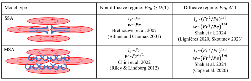
Figure 1: Illustrations and summary of the SSA and MSA model predictions for $w$ and $l_{z}$ in both the non-diffusive and diffusive regimes. Horizontal eddies are shown in red, and vertical eddies are shown in blue.

2 Comparison of theory with DNS

The SSA and MSA theories differ primarily in their predictions for the characteristic vertical length scale of the flow (or equivalently, $\alpha$) and for the characteristic vertical velocity. We are therefore interested in comparing these predictions to the data. In practice, however, the characteristic vertical length scale is a relatively difficult quantity to extract from the DNS, as there is no unique and universally-accepted definition. Consequently, we focus solely on comparing the theoretical predictions for the characteristic vertical velocity of the flow to the root-mean-square (rms) of the $w$ field because that quantity is both well-defined and easy to compute.

In what follows, we extend and re-analyze the datasets presented in Cope et al., (2020) and Garaud, (2020). Both studies performed DNS of the set of non-dimensional equations (1) with $\boldsymbol{F}_{h}=\sin(y)\boldsymbol{e}_{x}$ in a triply-periodic domain of size $4\pi\times 2\pi\times 2\pi$ using the PADDI code (Traxler et al.,, 2011). We focus on their highest Reynolds number simulations, which were performed for $Re=600$. Note that in this paper, Cope et al., (2020) and Garaud, (2020), $Re$ is defined using the inverse wavenumber of the forcing, and thus is a factor of $2\pi$ smaller than that of simulations which use the box size as the unit of length instead. Cope et al., (2020) presented a range of DNS for $Pe\leq 0.1$ and low $Fr$ (using the parameter $B=Fr^{-2}$ to characterize the stratification). They also ran a few simulations in the asymptotically low $Pe$ regime (Lignières,, 1999), called the LPN regime hereafter, where the buoyancy equation is replaced by $w=Pe^{-1}\nabla^{2}b$. Garaud, (2020) presented DNS with $Re=600$, $Pe=60$ (i.e. $Pr=0.1$) and low $Fr$. Each simulation was integrated until a statistically-stationary state was reached, lasting at least 100 time units. In some cases, we had to further extend the original DNS from Cope et al., (2020) or Garaud, (2020) to have a sufficiently long stationary time series. The quantity $w_{rms}=\langle w^{2}\rangle_{t}^{1/2}$, where $\langle\cdot\rangle_{t}$ denotes a volume and time average, was then measured in that statistically stationary state using the extended data.

To complement this dataset, we have run additional simulations at $Re=1000$, $Pe=100$. These DNS have twice the spatial resolution of those of Cope et al., (2020) and Garaud, (2020) and, thus, have only been integrated for up to 50 time units in the statistically stationary regime. In addition, the full fields are too large to be saved regularly, so we have saved two-dimensional slices through the data in the $(x,y)$, $(y,z)$ and $(x,z)$ planes. These simulations are only used for visualizations and to assess the influence of viscosity by comparison with the $Re=600$ results.

We compare the $w_{rms}$ data and the various theories in the top row of figure 2. The left panel shows $w_{rms}$ as a function of $Fr^{-1}$, measured for the $Pe=60$, $Re=600$ runs (green symbols), and for the $Pe=100$, $Re=1000$ runs (orange symbols). Note that $Pr=0.1$ in both cases. We refer to these simulations as ‘non-diffusive’ runs because $Pe$ is large. The fact that the measured values of $w_{rms}$ are identical for the two sets of simulations at different $Re$ demonstrates that viscous effects are negligible, at least for $Fr^{-1}\leq 20$. The right panel shows the results of the suite of experiments at $Pe=0.1$, $Re=600$ (purple symbols), for which $Pr=0.1/600$. We refer to these simulations as ‘diffusive’ runs, because $Pe$ is small. Note that some of these runs were actually integrated using the LPN regime equations instead (square symbols). In that case, the relevant input parameters are $Re$ and $\chi=Pe/Fr^{2}$ ($=BPe$ in the notation of Cope et al.,, 2020). To obtain the corresponding value of $Fr$ for a given $\chi$, simply note that $Fr=\sqrt{Pe/\chi}$ for a given $Pe$. Illustrated as well in the same plots are the various theoretical predictions for the vertical velocity: the red line in each panel corresponds to the SSA theory, while the blue line corresponds to the MSA theory.

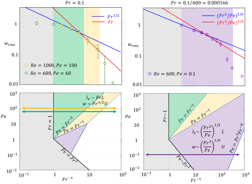
Figure 2: Top row: Comparison between the model predictions and the data for non-diffusive simulations with $Pr=0.1$ and two different values of $Re$ (left) and diffusive simulations with $Re=600$, $Pe=0.1$ (right). Symbols show $w_{rms}$ extracted from the DNS and errorbars show the standard deviation of its temporal variability. Squares on the right panel denote LPN simulations (see main text for details). The blue and red lines in each panel show the MSA and SSA scaling predictions, respectively. Bottom row: Regime diagrams for stratified turbulence at $Pr=0.1$ (left) and $Pr=0.1/600\simeq 0.00017$ (right), adapted from Shah et al., (2024). Grey regions support isotropic motions. White regions are viscously controlled ($Re_{b}\leq 1$). Green regions support non-diffusive anisotropic stratified turbulence ($Pe_{b}\geq\mathit{O}(1)$), and purple regions support diffusive anisotropic stratified turbulence ($Pe_{b}\ll\alpha$). The yellow regions are in the ‘intermediate’ regime of Shah et al., (2024) ($\mathit{O}(\alpha)\leq Pe_{b}\ll 1$). Horizontal arrows show the transects through the regimes corresponding to the panels above.

The bottom row of figure 2 shows for comparison the expected regime diagrams for the corresponding values of $Pr$ in each case, based on the asymptotic theory of Shah et al., (2024). The coloured horizontal arrows show the transect taken through parameter space for each series of DNS shown in the top row. The background colours show the expected regime: isotropic motions with $\alpha\simeq 1$ (grey), non-diffusive anisotropic turbulence (green), intermediate regime (yellow), diffusive anisotropic turbulence (violet) and viscous regime (white). The same background colours in the top row show the expected regime transitions as a function of $Fr^{-1}$ at the value of $Pe$ corresponding to the transect taken. We note that while Shah et al., (2024) distinguished the non-diffusive and intermediate regimes, these have the same predicted scalings for $\alpha$ and $w$; in any case, the intermediate regime does not span a large region of parameter space at $Pr=0.1$ and would be difficult to identify even if the scaling laws differed.

Examination of the top panels confirms that none of the theories applies when the stratification is weak so the flow is isotropic on all scales ($\alpha\simeq 1$, grey region), or in the viscous regime (white region), where $Re_{b}\leq 1$. This is, of course, as expected. However, we also see that neither the SSA nor the MSA model predictions fit the data in the entire region where they are supposedly valid (i.e. the green/yellow regions in the non-diffusive case, and the purple region in the diffusive case). Instead, we find that the MSA predictions appear to be better at weaker stratifications (higher $Fr$) while the SSA predictions appear to be better at higher stratification (lower $Fr$), when $Re$ is fixed.

3 The effects of intermittency

To gain insight into the applicability of the predicted scalings, we examine the actual flow field more closely. Figure 3 shows snapshots of $u$ and $w$ in two different high-resolution DNS at $Pe=100$ and $Re=1000$. The left panels show a more weakly stratified case with $Fr\simeq 0.18$ and the right panels show a more strongly stratified case with $Fr\simeq 0.058$. It is clear that while the $Fr\simeq 0.18$ case is fully turbulent, the more strongly stratified case is not, but exhibits instead spatial intermittency in as much as the turbulence is localized to small ‘patches’ (see e.g. the regions of high $|w|$ in the bottom right panel). Similar findings were reported by Cope et al., (2020) in their low $Pe$ simulations in the regime that they named ‘stratified intermittent’ (see their figure 6).

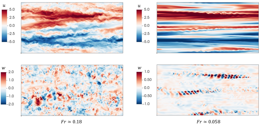
Figure 3: DNS snapshots of $u$ (top row) and $w$ (bottom row) in the $y=0$ plane for $Re=1000$, $Pe=100$. The left column shows a more weakly stratified simulation with $Fr=30^{-1/2}\simeq 0.18$ and the right column shows a more strongly stratified simulation with $Fr=300^{-1/2}\simeq 0.058$. Note the spatially intermittent nature of the turbulence in the latter.

These snapshots demonstrate two very important aspects of strongly stratified turbulence that have direct implications for asymptotic analyses. First, they illustrate the coexistence of large and small horizontal scales, with $u$ dominated by large scales with subdominant small scales, and $w$ dominated by small scales with subdominant large scales (cf. Riley and Lindborg,, 2012). This ordering is a cornerstone of the MSA theories of Chini et al., (2022) and Shah et al., (2024). Secondly, they show in the more strongly stratified case that these small horizontal scales are only dominant within the turbulent patches, and essentially disappear outside of these patches. As such, the distinct MSA model scalings are only expected to apply within the turbulent patches. In the more orderly layer-like flow outside of those patches, the SSA scalings—which coincide with the MSA model predictions in regions where small scales are not excited—should hold.

To verify this interpretation quantitatively, we sought to identify a reliable diagnostic for the turbulent patches, i.e. regions where the flow exhibits small horizontal scales. It is common to use the enstrophy $|{\boldsymbol{\omega}}|^{2}$ as a diagnostic for turbulence, where $\boldsymbol{\omega}=\nabla\times{\bf u}$ is the flow vorticity. Indeed, the turbulent cascade to small scales implies that enstrophy must be large within the patches. However, enstrophy turns out to be an inappropriate diagnostic for our purpose because it can also be large in the layer-like regions of strong vertical shear outside of the turbulent patches, such as the ones described by the SSA model. This fact is illustrated in figure 4(a), which shows the enstrophy field in a particular snapshot of a strongly stratified simulation, and can be understood as follows. According to Chini et al., (2022) and Shah et al., (2024), ${\boldsymbol{u}}=\bar{\boldsymbol{u}}+{\boldsymbol{u}}^{\prime}$ where $\bar{\boldsymbol{u}}$ can be thought of as the large-scale anisotropic component of the flow, which varies on the $O(1)$ horizontal scales and $O(\alpha)$ vertical scale, as in the SSA model. Meanwhile ${\boldsymbol{u}}^{\prime}$ can be thought of as the small-scale isotropic and turbulent component of the flow, which varies on $O(\alpha)$ scales in all directions, as in the MSA model. Furthermore, these authors show that $\bar{u}\sim\bar{v}\sim O(1)$, while $\bar{w}\sim O(\alpha)$, and $u^{\prime}\sim v^{\prime}\sim w^{\prime}\sim O(\alpha^{1/2})$. Accordingly, we find that the horizontal vorticity components are dominated by the contribution from $\bar{\boldsymbol{u}}$, namely $\omega_{x}\sim\bar{\omega}_{x}\sim\omega_{y}\sim\bar{\omega}_{y}\sim O(Fr^{-1})$, while the vertical vorticity component is dominated by the contributions from ${\boldsymbol{u}}^{\prime}$, with $\omega_{z}\sim\omega^{\prime}_{z}\sim O(Fr^{-1/2})$. As a result, we argue that $\omega_{z}^{2}$ is a more reliable diagnostic of the small-scale turbulence than the enstrophy. This assertion is confirmed in figure 4(b), which shows $\omega_{z}^{2}$ for the same snapshot depicted in figure 4(a). We see that the regions of high $\omega_{z}^{2}$ only highlight the turbulent patches of the flow.

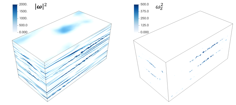
Figure 4: Snapshots of enstrophy (left) and vertical vorticity squared (right) from a simulation at $Re=600$, $Pe=60$, and $Fr=0.05$. The latter is a better diagnostic of the turbulent patches.

In what follows, we therefore define the following quantities:

$$w^{\rm turb}_{rms}=\frac{\langle w^{2}\omega_{z}^{2}\rangle_{t}^{1/2}}{\langle\omega_{z}^{2}\rangle_{t}^{1/2}},\quad\mbox{ and }\quad w^{\rm noturb}_{rms}=\frac{\langle w^{2}\omega_{z}^{-2}\rangle_{t}^{1/2}}{\langle\omega_{z}^{-2}\rangle_{t}^{1/2}}.$$ (4)

The first can essentially be viewed as the root-mean-square of $w$ taken over the turbulent patches, where the distinct MSA scalings should apply. The second can be viewed as the rms of $w$ taken everywhere other than the turbulent patches, where the SSA scalings should apply. Note that the computation of $w^{\rm turb}_{rms}$ and $w^{\rm noturb}_{rms}$ requires integrals of $w^{2}$, $\omega_{z}^{2}$, and their product or ratio over the entire volume, which was not one of the simulation diagnostics originally saved. As such, we are unable to extract these quantities from the $Re=1000$ simulations. However, we can compute them from the full-data snapshots regularly saved in the $Re=600$ simulations in both high and low $Pe$ datasets (of which there are usually between 50 and 100 depending on the simulation). The variance is naturally larger than for the $w_{rms}$ data, owing to the intermittency of the turbulence.

We present the results in figure 5, with the non-diffusive $Re=600,Pe=60$ simulations on the left and the diffusive $Re=600,Pe=0.1$ simulations on the right. The background colours are the same as in figure 2. The $w_{rms}$ data from figure 2 is again shown in green and purple symbols. We plot the $w^{\rm turb}_{rms}$ data using blue symbols in both cases, and the MSA scalings for turbulent regions using a blue line for comparison. Similarly, we plot the $w^{\rm noturb}_{rms}$ data using red symbols and the SSA scalings using a red line. We see, quite clearly, that each theory fits the data in its respective region of validity—the distinct MSA scalings being valid in the turbulent patches, and the SSA scalings only being valid outside of the turbulent patches. This shows that the transition observed in figure 2, from simulations that appear to satisfy the turbulent MSA scalings better at low stratification to simulations that appear to fit the SSA scalings better at high stratification, primarily is a consequence of the decrease in the volumetric fraction of the domain occupied by the turbulent patches when $Fr^{-1}$ increases.

As the stratification continues to increase, the buoyancy Reynolds number $Re_{b}=\alpha^{2}Re$ eventually decreases below a critical value $Re_{b,{\rm crit}}=O(1)$, where viscous effects become dominant. Assuming $Re_{b,{\rm crit}}=1$, we show this transition in figure 2 as the line separating the coloured area from the white region, for the MSA model. In the non-diffusive case (left panel), $\alpha=Fr$, so $Re_{b}=1$ is equivalent to $Pe=PrFr^{-2}$, which is the edge of the yellow region. We see that the data are consistent with this prediction: beyond the viscous transition, $w_{rms}$ rapidly drops to very low values consistent with a viscously-dominated flow. For the diffusive case (right panel), $\alpha=(Fr^{2}/Pe)^{1/3}$ in the MSA model so $Re_{b}=1$ is equivalent to $Pe=Pr^{3}Fr^{-4}$, which corresponds to the edge of the purple region. We see that the effects of viscosity appear to become important at slightly weaker stratification than predicted assuming $Re_{b,{\rm crit}}=1$, but plausibly attribute this discrepancy to missing $O(1)$ constants in the estimates for $\alpha$ and/or $Re_{b,{\rm crit}}$.

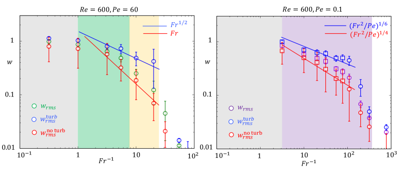
Figure 5: Comparison between models and data for the characteristic vertical velocity at $Re=600$, $Pe=60$ (left) and at $Re=600$, $Pe=0.1$ (right). Green and purple symbols show $w_{rms}$ in the left and right panels, respectively. In both panels, blue symbols show $w^{\rm turb}_{rms}$ and should be compared with the turbulent MSA scalings (blue lines), while red symbols show $w^{\rm noturb}_{rms}$ and should be compared with the corresponding SSA scalings (red lines).

4 Conclusion

In this paper, we have presented a detailed comparison of DNS data with various theoretical predictions for the characteristic vertical velocity of fluid motions in forced stratified turbulence. In particular, we have studied both moderate and low Prandtl number regimes, resulting in a wide range of Péclet numbers at fixed Reynolds number. When buoyancy diffusion is negligible, our results notably provide compelling evidence for the $w\propto Fr^{1/2}$ scaling law for stratified turbulence first proposed by Riley and Lindborg, (2012) using heuristic arguments and rigorously derived by Chini et al., (2022) using multiscale asymptotic analysis. In the latter investigation, this scaling law is intrinsically tied to the existence of small-scale isotropic flow motions driven by the emergent vertical shear between larger-scale primarily horizontal eddies, as corroborated by the results from the DNS presented here. The vertical shear instability is gradually stabilized as the buoyancy Reynolds number decreases towards a critical value of order unity, and the small-scale isotropic component of the turbulence becomes spatio-temporally intermittent rather than domain filling. Outside of the turbulent patches, small horizontal scales disappear, and we find that $w\propto Fr$ instead, consistent with the model of Billant and Chomaz, (2001) and Brethouwer et al., (2007). In this intermittent regime, therefore, the rms vertical velocity of the flow computed from an average over the whole domain differs from either of these scaling laws, and additionally depends on the volume filling factor of the small-scale turbulence, whose dependence on stratification will be the subject of future work. This intermittency also explains the incorrect conclusion reached by Garaud, (2020) regarding the possible existence of another regime of stratified turbulence where $w\propto Fr^{2/3}$. In hindsight, we understand her empirically-inferred scaling simply as a consequence of the decrease in the volume filled by turbulent patches with increasing stratification at fixed $Re$.

At low $Pr$, Shah et al., (2024) revised the predictions of Brethouwer et al., (2007) and Chini et al., (2022) to account for the effects of buoyancy diffusion. They showed that the presence of small isotropic motions implies that $w\propto(Fr^{2}/Pe)^{1/6}$, consistent with an early model and DNS data by Cope et al., (2020), while in their absence $w\propto(Fr^{2}/Pe)^{1/4}$, consistent with predictions from Lignières, (2020) and Skoutnev, (2023). Revisiting the very low $Pr$ DNS of Cope et al., (2020) in this new light, we have confirmed both scaling laws within and outside of the turbulent patches, respectively. Finally, the models of Chini et al., (2022) and Shah et al., (2024) also predict where in parameter space viscous effects become important. We have confirmed these predictions, too, with our DNS data.

In summary, this investigation demonstrates that the combination of rigorous multiscale analysis (Chini et al.,, 2022; Shah et al.,, 2024) with idealized DNS (Cope et al.,, 2020; Garaud,, 2020, and new simulations presented here) can be a powerful tool to identify and validate scaling laws for stratified turbulence across different regions of parameter space. In future work, we will incorporate the effects of rotation and magnetic fields, which must be taken into account for a more realistic description of stratified turbulence in geophysical and astrophysical settings.

Declaration of Interests

The authors report no conflict of interest.

References

- Billant and Chomaz, (2001) Billant, P. and Chomaz, J.-M. (2001). Self-similarity of strongly stratified inviscid flows. Phys. Fluids, 13(6):1645–1651.
- Brethouwer et al., (2007) Brethouwer, G., Billant, P., Lindborg, E., and Chomaz, J.-M. (2007). Scaling analysis and simulation of strongly stratified turbulent flows. J. Fluid Mech., 585:343–368.
- Chini et al., (2022) Chini, G., Michel, G., Julien, K., Rocha, C., and Caulfield, C. (2022). Exploiting self-organized criticality in strongly stratified turbulence. J. Fluid Mech., 933:A22.
- Cope et al., (2020) Cope, L., Garaud, P., and Caulfield, C. (2020). The dynamics of stratified horizontal shear flows at low Péclet number. J. Fluid Mech., 903:A1.
- Garaud, (2020) Garaud, P. (2020). Horizontal shear instabilities at low Prandtl number. Astrophys. J., 901(2).
- Klein, (2010) Klein, R. (2010). Scale-dependent models for atmospheric flows. Annu. Rev. Fluid Mech., 42:249–274.
- Lignières, (1999) Lignières, F. (1999). The small-Péclet-number approximation in stellar radiative zones. Astro. Astrophys., 348:933–939.
- Lignières, (2020) Lignières, F. (2020). Turbulence in stably stratified radiative zone. In Multi-Dimensional Processes In Stellar Physics, pages 111–140.
- Maffioli and Davidson, (2016) Maffioli, A. and Davidson, P. (2016). Dynamics of stratified turbulence decaying from a high buoyancy Reynolds number. J. Fluid Mech., 786:210–233.
- Riley and Lindborg, (2012) Riley, J. J. and Lindborg, E. (2012). Recent Progress in Stratified Turbulence in Ten Chapters in Turbulence, ed. Davidson, P. A., Kaneda, Y. & Sreenivasan, K. R. , page 269–317. Cambridge University Press.
- Shah et al., (2024) Shah, K., Chini, G. P., Caulfield, C. P., and Garaud, P. (2024). Regimes of stratified turbulence at low Prandtl number. submitted to J. Fluid Mech.
- Skoutnev, (2023) Skoutnev, V. (2023). Critical balance and scaling of strongly stratified turbulence at low Prandtl number. J. Fluid Mech., 956:A7.
- Traxler et al., (2011) Traxler, A., Stellmach, S., Garaud, P., Radko, T., and Brummell, N. (2011). Dynamics of fingering convection. Part 1 Small-scale fluxes and large-scale instabilities. J. Fluid Mech., 677:530–553.