Learning Heuristics for Transit Network Design and Improvement with Deep Reinforcement Learning

Abstract

Transit agencies world-wide face tightening budgets. To maintain quality of service while cutting costs, efficient transit network design is essential. But planning a network of public transit routes is a challenging optimization problem. The most successful approaches to date use metaheuristic algorithms to search through the space of possible transit networks by applying low-level heuristics that randomly alter routes in a network. The design of these low-level heuristics has a major impact on the quality of the result. In this paper we use deep reinforcement learning with graph neural nets to learn low-level heuristics for an evolutionary algorithm, instead of designing them manually. These learned heuristics improve the algorithm’s results on benchmark synthetic cities with 70 nodes or more, and obtain state-of-the-art results when optimizing operating costs. They also improve upon a simulation of the real transit network in the city of Laval, Canada, by as much as 54% and 18% on two key metrics, and offer cost savings of up to 12% over the city’s existing transit network.

1 INTRODUCTION

The COVID-19 pandemic resulted in declines in transit ridership in cities worldwide (Liu et al., 2020). This has led to a financial crisis for municipal transit agencies, putting them under pressure to reduce transit operating costs (Kar et al., 2022). But if cost-cutting leads to reduced quality of service, ridership may be harmed further, leading to a downward spiral of service quality and income. Agencies find themselves having to do more with less. Thus, the layout of transit networks is key, as a well-planned layout can cut operating costs and improve service quality. But changes to a transit network are not to be made lightly. For rail transit, it can require infrastructural changes that may be prohibitive. And even for bus transit, network redesigns can be costly and disruptive for users and bus drivers. So it is vital to agencies that they get network design or modification right the first time. Good algorithms for the transit network design problem (NDP) can therefore be very useful to transit agencies.

The NDP is the problem of designing a set of transit routes for a city that satisfy one or more objectives, such as meeting all travel demand and minimizing operating costs. It is an NP-complete problem that has commonalities with the travelling salesman problem (TSP) and vehicle routing problem (VRP), but is more complex than these famously-challenging problems. Since real-world cities typically have hundreds or even thousands of possible stop locations, analytical optimization approaches are infeasible. For this reason, the most successful approaches to the NDP to-date have been metaheuristic algorithms. Most such algorithms work by repeatedly applying one or more low-level heuristics that randomly modify a network, guiding this random walk towards better networks over many iterations by means of a metaheuristic such as natural selection (as in evolutionary algorithms) or metallic annealing (as in simulated annealing). Many different metaheuristics for guiding the search have been proposed, as have a range of low-level heuristics for transit network design specifically. While these algorithms can find good solutions in many cases, real-world transit networks are still commonly designed by hand (Durán-Micco and Vansteenwegen, 2022).

The different low-level heuristics used in these metaheuristic algorithms make different kinds of alterations: one heuristic may randomly select a stop on an existing route and remove it from the route, while another may randomly add a stop at one end of a route, and another may select two stops on a route at random and exchange them. What most low-level heuristics have in common is that they are uniformly random: no aspect of the particular network or city affects the heuristic’s likelihood making one change versus another. We here wish to consider whether a machine learning system could act as a more intelligent heuristic, by learning to use information about the city and the current transit network to make only the most promising changes.

In our prior work (Holliday and Dudek, 2023), we trained a graph neural net (GNN) to plan a transit network from scratch, and showed that using this to generate an initial transit network improved the quality of networks found by two metaheuristic algorithms. That policy assembled transit routes by concatenating shortest paths in the city’s street network that share end-points, using the neural net to select the next shortest path to be included at each step. By repeating this process for each route that is needed, it assembled a complete transit network.

Our subsequent work (Holliday and Dudek, 2024) built on this by considering whether the GNN can benefit a metaheuristic algorithm by serving as a learned low-level heuristic. To test this, we modified an existing evolutionary algorithm (Nikolić and Teodorović, 2013), replacing one of its low-level heuristics with a heuristic that applies the GNN to plan one new route. We found that this learned heuristic considerably improved the algorithm’s performance on cities with 70 nodes or more.

In the present work, we expand on those results in several ways. We present new results obtained with an improved GNN model and an improved evolutionary algorithm. We also perform ablation studies to analyze the importance of different components of our neural-evolutionary hybrid algorithm. As part of these ablations, we consider a novel unlearned low-level heuristic, where shortest paths with common end-points are joined uniformly at random instead of according to the GNN’s output. Interestingly, we find that in the narrow case where we are only concerned with minimizing passenger travel time, this heuristic outperforms both the baseline heuristics of Nikolić and Teodorović (2013) and our GNN heuristic; in most other cases, however, our GNN heuristic performs better.

We compare the performance of our learned and unlearned heuristics with other results on the widely-used Mandl (Mandl, 1980) and Mumford (Mumford, 2013a) benchmark cities. We find that the unlearned heuristic obtains results comparable to the state of the art when minimizing only the passengers’ travel time, while the GNN heuristic outperforms the previous state of the art by as much as 13% when minimizing only the cost to operators.

Finally, we go beyond our earlier work by applying our heuristics to real data from the city of Laval, Canada, a very large real-world problem instance. We show that our learned heuristic can be used to plan transit networks for Laval that, in simulation, exceed the performance of the city’s existing transit system by a wide margin, for three distinct optimization goals. These results show that learned GNN heuristics may allow transit agencies to offer better service at less cost.

2 BACKGROUND AND RELATED WORK

2.1 Deep Learning for Optimization Problems

Deep learning refers to machine learning techniques that involve “deep” artificial neural nets - that is, neural nets with many hidden layers. Deep reinforcement learning refers to the use of deep neural nets in reinforcement learning (RL). RL is a branch of machine learning in which a learning system, such as a neural net, chooses actions and receives a numerical “reward” for each action, and learns to choose actions that maximize total reward. As documented by  Bengio et al. (2021), there is growing interest in the application of deep learning, and deep RL specifically, to combinatorial optimization (CO) problems such as the TSP.

Vinyals et al. (2015) proposed a deep neural net model called a Pointer Network, and trained it via supervised learning to solve TSP instances. Subsequent work, such as that of Dai et al. (2017), Kool et al. (2019), and Sykora et al. (2020), has built on this. These works use similar neural net models, in combination with reinforcement learning algorithms, to train neural nets to construct CO solutions. These have attained impressive performance on the TSP, the VRP, and other CO problems. More recently, Mundhenk et al. (2021) train an recurrent neural net (RNN) via RL to construct a starting population of solutions to a genetic algorithm, the outputs of which are used to further train the RNN. Fu et al. (2021) train a model on small TSP instances and present an algorithm that applies the model to much larger instances. Choo et al. (2022) present a hybrid algorithm of Monte Carlo Tree Search and Beam Search that draws better sample solutions for the TSP and Capacitated (CVRP) from a neural net policy like that of Kool et al. (2019).

These approaches all belong to the family of “construction” methods, which solve a CO problem by starting with an “empty” solution and adding to it until it is complete - for example, in the TSP, this would mean constructing a path one node at a time, starting with an empty path and stopping once the path includes all nodes. The solutions from these neural construction methods come close to the quality of those from specialized algorithms such as Concorde (Applegate et al., 2001), while requiring much less run-time to compute (Kool et al., 2019).

By contrast with construction methods, “improvement” methods start with a complete solution and repeatedly modify it, searching through the solution space for improvements. In the TSP example, this might involve starting with a complete path, and swapping pairs of nodes in the path at each step to see if the path is shortened. Improvement methods are generally more computationally costly than construction methods but can yield better results. Evolutionary algorithms belong to this category.

Some work has considered training neural nets to choose the search moves to be made at each step of an improvement method (Hottung and Tierney, 2019; Chen and Tian, 2019; d O Costa et al., 2020; Wu et al., 2021; Ma et al., 2021), and Kim et al. (2021) train one neural net to construct a set of initial solutions, and another to modify and improve them. This work has shown impressive performance on the TSP and other CO problems. Our work belongs to this family, in that we train a neural net to solve instances of the transit network design problem, and then use it to modify solutions within an improvement method.

In most of the above work, the neural net models used are graph neural nets, a type of neural net model that is designed to operate on graph-structured data (Bruna et al., 2013; Kipf and Welling, 2016; Defferrard et al., 2016; Duvenaud et al., 2015). These have been applied in many other domains, including the analysis of large web graphs (Ying et al., 2018), the design of printed circuit boards (Mirhoseini et al., 2021), and the prediction of chemical properties of molecules (Duvenaud et al., 2015; Gilmer et al., 2017). An overview of GNNs is provided by Battaglia et al. (2018). Like many CO problems, the transit network design problem lends itself to being described as a graph problem, so we use GNN models here as well.

In most CO problems, it is difficult to find globally optimal solutions but easier gauge the quality of a given solution. As  Bengio et al. (2021) note, this makes reinforcement learning a natural fit to CO problems. Most of the work cited in this section uses RL methods to train neural net models. We do the same here, applying a method similar to that of Kool et al. (2019) to the NDP.

2.2 Optimization of Public Transit

The NDP is an NP-complete problem (Quak, 2003), meaning that it is impractical to find optimal solutions for most cases. While analytical optimization and mathematical programming methods have been successful on small instances (van Nes, 2003; Guan et al., 2006), they struggle to realistically represent the problem (Guihaire and Hao, 2008; Kepaptsoglou and Karlaftis, 2009). Metaheuristic approaches, as defined by Sörensen et al. (2018), have thus been more widely applied.

The most widely-used metaheuristics for the NDP have been genetic algorithms, simulated annealing, and ant-colony optimization, along with hybrids of these methods (Guihaire and Hao, 2008; Kepaptsoglou and Karlaftis, 2009; Durán-Micco and Vansteenwegen, 2022; Yang and Jiang, 2020; Hüsselmann et al., 2023). Recent work has also shown other metaheuristics can be used with success, such as sequence-based selection hyper-heuristics (Ahmed et al., 2019), beam search (Islam et al., 2019), and particle swarms (Lin and Tang, 2022). Many different low-level heuristics have been applied within these metaheuristic algorithms, but most have in common that they select among possible neighbourhood moves uniformly at random.

One exception is Hüsselmann et al. (2023). For two heuristics, the authors design a simple model of how each change the heuristic could make would affect solution quality. They use this model to give the different changes different probabilities of being selected. The resulting heuristics obtain state-of-the-art results. However, their simple model ignores passenger trips involving transfers, and the impact of the user’s preferences over different parts of the cost function. By contrast, the method we propose learns a model of changes’ impacts to assign probabilities to those changes, and does so based on a richer set of inputs.

While neural nets have often been used for predictive problems in urban mobility (Xiong and Schneider, 1992; Rodrigue, 1997; Chien et al., 2002; Jeong and Rilett, 2004; Çodur and Tortum, 2009; Li et al., 2020) and for other transit optimization problems such as scheduling, passenger flow control, and traffic signal control (Zou et al., 2006; Ai et al., 2022; Yan et al., 2023; Jiang et al., 2018; Wang et al., 2024), they have not often been applied to the NDP, and neither has RL. Two recent examples are Darwish et al. (2020) and Yoo et al. (2023). Both use RL to design routes and a schedule for the Mandl benchmark (Mandl, 1980), a single small city with just 15 transit stops, and both obtain good results. Darwish et al. (2020) use a GNN approach inspired by Kool et al. (2019); in our own work we experimented with a nearly identical approach to Darwish et al. (2020), but found it did not scale beyond very small instances. Meanwhile, Yoo et al. (2023) use tabular RL, a type of approach which is practical only for small problem sizes. Both of these approaches also require a new model to be trained on each problem instance. Our approach, by contrast, is able to find good solutions for NDP instances of more than 600 nodes, and can be applied to instances unseen during model training.

3 TRANSIT NETWORK DESIGN PROBLEM

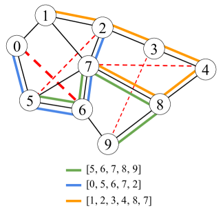
Figure 1: An example city graph with ten numbered nodes and three routes. Street edges are black, routes are in colour, and demands are shown by dashed red lines. The edges of the three routes form a subgraph of the street graph $(\mathcal{N},\mathcal{E}_{s})$. All node-pairs with demand are connected by this subgraph, so the three routes form a valid transit network. The demand between nodes 2 and 5 and between 0 and 6 can be satisfied directly by riding on the blue line, and the demand from 7 to 4 by the orange line. But the demand from 3 to 9 requires one transfer: passengers must ride the orange line from node 3 to 8, and then the green line from node 8 to 9.

In the transit network design problem, one is given an augmented graph that represents a city:

$$\mathcal{C}=(\mathcal{N},\mathcal{E}_{s},D)$$ (1)

This is comprised of a set $\mathcal{N}$ of $n$ nodes, representing candidate stop locations; a set $\mathcal{E}_{s}$ of street edges $(i,j,\tau_{ij})$ connecting the nodes, with weights $\tau_{ij}$ indicating drive times on those streets; and an $n\times n$ Origin-Destination (OD) matrix $D$ giving the travel demand, in number of trips, between every pair of nodes in $\mathcal{N}$. The goal is to propose a transit network, which is a set of routes $\mathcal{R}$ that minimizes a cost function $C:\mathcal{C},\mathcal{R}\rightarrow\mathbb{R}^{+}$, where each route $r\in\mathcal{R}$ is a sequence of nodes in $\mathcal{N}$. The transit network $\mathcal{R}$ is subject to the following constraints:

1. $\mathcal{R}$ must satsify all demand, providing some path over transit between every pair of nodes $(i,j)\in\mathcal{N}$ for which $D_{ij}>0$.

2. $\mathcal{R}$ must contain exactly $S$ routes ($|\mathcal{R}|=S$), where $S$ is a parameter set by the user.

3. All routes $r\in\mathcal{R}$ must obey the same limits on its number of stops: $MIN\leq|r|\leq MAX$, where $MIN$ and $MAX$ are parameters set by the user.

4. Routes $r\in\mathcal{R}$ must not contain cycles; each node $i\in\mathcal{N}$ can appear in $r$ at most once.

We here deal with the symmetric NDP, meaning that all demand, streets, and routes are the same in both directions. This means $D=D^{\top}$, $(i,j,\tau_{ij})\in\mathcal{E}_{s}$ iff. $(j,i,\tau_{ij})\in\mathcal{E}_{s}$, and all routes are traversed both forwards and backwards by vehicles on them. An example city graph with a transit network is shown in Figure 1.

3.1 Markov Decision Process Formulation

A Markov Decision Process (MDP) is a formalism commonly used to define problems in RL (Sutton and Barto, 2018, Chapter 3). In an MDP, an agent interacts with an environment over a series of timesteps $t$, starting at $t=0$. At each timestep $t$, the environment is in a state $s_{t}\in\mathcal{S}$, and the agent observes the state and takes some action $a_{t}\in\mathcal{A}_{t}$, where $\mathcal{A}_{t}$ is the set of available actions at that timestep. The environment then transitions to a new state $s_{t+1}\in\mathcal{S}$ according to the state transition distribution $P(s_{t+1}|s_{t},a_{t})$, and the agent receives a numerical reward $R_{t}\in\mathbb{R}$ according to the reward distribution $P(R_{t}|s_{t},a_{t},s_{t+1})$. The agent chooses actions according to its policy $\pi(a_{t}|s_{t})$, which is a probability distribution over $\mathcal{A}_{t}$ given $s_{t}$. In RL, the goal is usually to learn a policy $\pi$ that maximizes the return $G_{t}$, defined as a time-discounted sum of rewards:

$$G_{t}=\sum^{t_{\text{end}}}_{t^{\prime}=t}\gamma^{t^{\prime}-t}R_{t^{\prime}}$$ (2)

Where $\gamma\in[0,1]$ is a parameter that discounts rewards farther in the future, and $t_{\text{end}}$ is the final time-step of the MDP. The sequence of states visited, actions taken, and rewards received from $t=0$ to $t_{\text{end}}$ constitutes one episode of the MDP.

We here describe the MDP we use to represent a construction approach to the transit network design problem. As shown in Equation 3, the state $s_{t}$ is composed of the set of finished routes $\mathcal{R}_{t}$, and an in-progress route $r_{t}$ which is currently being planned.

$$s_{t}=(\mathcal{R}_{t},r_{t})$$ (3)

The starting state is $s_{0}=(\mathcal{R}_{0}=\{\},r_{0}=[])$. At a high level, the MDP alternates at every timestep between two modes: on odd-numbered timesteps, the agent selects an extension to the route $r_{t}$ that it is currently planning; on even-numbered timesteps, the agent chooses whether or not to stop extending $r_{t}$ and add it to the set of finished routes.

On odd-numbered timesteps, the available actions are drawn from SP, the set of shortest paths between all pairs of nodes in $\mathcal{C}$. If $r_{t}=[]$, then:

$$\mathcal{A}_{t}=\{a\;|\;a\in\textup{SP},|a|\leq MAX\}$$ (4)

Otherwise, $\mathcal{A}_{t}=\text{EX}_{r_{t}}$, where $\text{EX}_{r_{t}}$ is the set of paths $a\in\textup{SP}$ that satisfy all of the following conditions:

• $(i,j,\tau_{ij})\in\mathcal{E}_{s}$, where $i$ is the first node of $a$ and $j$ is the last node of $r_{t}$, or vice-versa

• $a$ and $r_{t}$ have no nodes in common

• $|a|\leq MAX-|r_{t}|$

Once a path $a_{t}\in\mathcal{A}_{t}$ is chosen, $r_{t+1}$ is formed by appending $a_{t}$ to the beginning or end of $r_{t}$ as appropriate.

On even-numbered timesteps, the action space depends on the number of stops in $r_{t}$:

$$\mathcal{A}_{t}=\begin{cases}\{\textup{continue}\}&\text{if}|r_{t}|<MIN\\ \{\textup{halt}\}&\text{if}|r_{t}|=MAX\text{ or }|\text{EX}_{r_{t}}|=0\\ \{\textup{continue},\textup{halt}\}&\text{otherwise}\end{cases}$$ (5)

If $a_{t}=\textup{halt}$, $r_{t}$ is added to $\mathcal{R}_{t}$ to get $\mathcal{R}_{t+1}=\mathcal{R}_{t}\cup\{r_{t}\}$, and $r_{t+1}=[]$ is a new empty route. If $a_{t}=\textup{continue}$, then $\mathcal{R}_{t+1}=\mathcal{R}_{t}$ and $r_{t+1}=r_{t}$.

The episode ends when the $S$-th route is added to $\mathcal{R}$: that is, if $|\mathcal{R}_{t+1}|=S$, the episode ends at timestep $t$. The output transit network is set to $\mathcal{R}=\mathcal{R}_{t+1}$, and the final reward is $R_{t_{\text{end}}}=-C(\mathcal{C},\mathcal{R})$. At all prior steps, $R_{t}=0$.

This MDP formalization imposes some helpful biases on the space of solutions. First, it requires any route connecting $i$ and $j$ to stop at all nodes along some path between $i$ and $j$, biasing planned routes towards covering more nodes. Second, it biases routes towards directness by forcing them to be composed of shortest paths. While an agent may construct arbitrarily indirect routes by choosing paths with length 2 at every step, this is unlikely because in a realistic street graph, the majority of paths in SP are longer than two nodes. Third, the alternation between deciding to continue or halt a route and deciding how to extend the route means that the probability of halting does not depend on how many different extensions are available; so a policy learned in environments with fewer extensions should generalize more easily to environments with more, and vice versa.

3.2 Cost Function

Our NDP cost function has three components. The cost to passengers, $C_{p}$, is the average passenger trip time over the network:

$$C_{p}(\mathcal{C},\mathcal{R})=\frac{\sum_{i,j}D_{ij}\tau_{\mathcal{R}ij}}{\sum_{i,j}D_{ij}}$$ (6)

Where $\tau_{\mathcal{R}ij}$ is the time of the shortest transit trip from $i$ to $j$ given $\mathcal{R}$, including a time penalty $p_{T}$ for each transfer the rider must make between routes.

The operating cost is the total driving time of the routes, or total route time:

$$C_{o}(\mathcal{C},\mathcal{R})=\sum_{r\in\mathcal{R}}\tau_{r}$$ (7)

Where $\tau_{r}$ is the time needed to completely traverse a route $r$ in one direction.

To enforce the constraints on $\mathcal{R}$, we use a third term $C_{c}$, which is the fraction of node pairs $(i,j)$ with $D_{ij}>0$ that are not connected by $\mathcal{R}$, plus a measure of by how many stops $|r|>MAX$ or $|r|<MIN$ across all routes. The cost function is then:

$$C(\mathcal{C},\mathcal{R})=\alpha w_{p}C_{p}+(1-\alpha)w_{o}C_{o}+\beta C_{c}$$ (8)

The weight $\alpha\in[0,1]$ controls the trade-off between passenger and operating costs, while $\beta$ is the penalty assigned for each constraint violation. $w_{p}$ and $w_{o}$ are re-scaling constants chosen so that $w_{p}C_{p}$ and $w_{o}C_{o}$ both vary roughly over the range $[0,1)$ for different $\mathcal{C}$ and $\mathcal{R}$; this is done so that $\alpha$ will properly balance the two, and to stabilize training of the GNN policy. The values used are $w_{p}=(\max_{i,j}T_{ij})^{-1}$ and $w_{o}=(S\max_{i,j}T_{ij})^{-1}$, where $T$ is an $n\times n$ matrix of shortest-path driving times between every node pair.

4 NEURAL NET HEURISTICS

4.1 Learning to Construct a Network

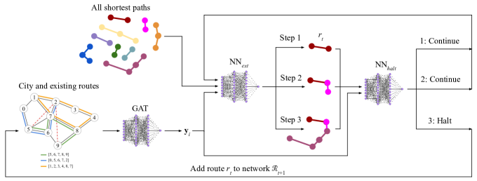
Figure 2: A schematic of our proposed route-planning method, outlining the route-construction MDP and showing the role of the policy network’s three components: the GAT backbone, $\textup{NN}_{ext}$, and $\textup{NN}_{halt}$.

In order to learn heuristics for transit network design, we first train a GNN policy $\pi_{\theta}(a|s)$, parameterized by $\theta$, to maximize the cumulative return $G_{t}$ on the construction MDP described in subsection 3.1. By then following this learned policy on the MDP for some city $\mathcal{C}$, stochastically sampling $a_{t}$ at each step with probabilities given by $\pi(\cdot|s_{t})$, we can obtain a transit network $\mathcal{R}$ for that city. We refer to this construction algorithm using the learned policy as “learned construction”. Because learned construction stochastically samples actions, we can run it multiple times to generate multiple networks for a city, and then pick the lowest-cost one. We will often do this by running learned construction 100 times and choosing the best network; we denote this procedure “LC-100”.

The central component of the policy net is a graph attention net (GAT) (Brody et al., 2021) which treats the city as a fully-connected graph on the nodes $\mathcal{N}$. Each node has an associated feature vector $\mathbf{x}_{i}$, and each edge a feature vector $\mathbf{e}_{ij}$, containing information about location, demand, existing transit connections, and the street edge (if one exists) between $i$ and $j$. We note that a graph attention net operating on a fully-connected graph has close parallels to a Transformer model (Vaswani et al., 2017), but unlike a Transformer, this architecture enables the use of edge features that describe known relationships between elements.

The GAT outputs node embeddings $\mathbf{y}_{i}$, which are operated on by one of two “head” neural nets, depending on the timestep: $\textup{NN}_{ext}$ for choosing among extensions when the timestep $t$ is odd, and $\textup{NN}_{halt}$ for deciding whether to halt when $t$ is even. Figure 2 is a schematic illustration of the function of each of these three components in the route-planning MDP. The full details of the neural architecture are presented in Appendix A. We have released the code for our method and experiments to the public.

4.1.1 Training

Following the work of Kool et al. (2019), we train the policy net using REINFORCE with baseline, a policy gradient method proposed by Williams (1992), and set $\gamma=1$. Since, by construction, the reward $R_{t}=0$ except at $t_{\text{end}}$, this implies the return $G_{t}$ is the same for all steps:

$$G_{t}=\sum^{t_{\text{end}}}_{t^{\prime}}R_{t^{\prime}}=-C(\mathcal{C},\mathcal{R})$$ (9)

The learning signal for each action $a_{t}$ is $L_{t}=G_{t}-b(s_{t})$, where the baseline $b(s_{t})$ is a learned quantity that estimates the average $G_{t}$ achieved by $\pi_{\theta}$ starting in state $s_{t}$. Differing from Kool et al. (2019), we compute the baseline at each step using a small Multi-Layer Perceptron (MLP) neural net that is separate from the $\pi_{\theta}$. This baseline net is trained to predict $G_{t}$ based on the cost weight parameter $\alpha$ and statistics of the city $\mathcal{C}$.

We train the policy net on a dataset of synthetic cities. We sample a different $\alpha\sim[0,1]$ for each city, while holding $S,MIN,MAX$, and the constraint weight $\beta$ constant across training. The values of these parameters used are presented in Table 7. At each iteration, a full MDP episode is run on a “batch” of cities from the dataset, $C(\mathcal{C},\mathcal{R})$, $b(s_{t})$ and $L_{t}$ are computed across the batch, and back-propagation and parameter updates are applied to both the policy net (taking the gradient with respect to $-L_{t}\ln\pi_{\theta}$) and the baseline net (taking the gradient with respect to the mean squared error between $G_{t}$ and $b(s_{t})$).

To construct a synthetic city for the training dataset, we first generate its nodes and street network using one of these processes chosen at random:

• $4$-nn: Sample $n$ random 2D points uniformly in a square to give $\mathcal{N}$. Add street edges to each node $i$ from its four nearest neighbours.

• 4-grid: Place $n$ nodes in a rectangular grid as close to square as possible. Add edges between all horizontal and vertical neighbour nodes.

• 8-grid: The same as 4-grid, but also add edges between diagonal neighbour nodes.

• Voronoi: Sample $m$ random 2D points in a square, and compute their Voronoi diagram (Fortune, 1995). Take the shared vertices and edges of the resulting Voronoi cells as $\mathcal{N}$ and $\mathcal{E}_{s}$. $m$ is chosen so $|\mathcal{N}|=n$.

For each process except Voronoi, each edge in $\mathcal{E}_{s}$ is then deleted with probability $\rho$. If the resulting street graph is not strongly connected, it is discarded and the process is repeated.

To generate our training dataset, we set $n=20$ and $\rho=0.3$, sample nodes (or the $m$ points for Voronoi) in a $30\textup{km}\times 30\textup{km}$ square, and assume a fixed vehicle speed of $v=15\textup{m/s}$ to compute street edge weights $\tau_{ij}=||(x_{i},y_{i})-(x_{j},y_{j})||_{2}/v$. Finally, we generate the OD matrix $D$ by setting diagonal demands $D_{ii}=0$, uniformly sampling above-diagonal elements $D_{ij}$ in the range $[60,800]$, and then setting below-diagonal elements $D_{ji}=D_{ij}$ to make $D$ symmetric. The dataset is composed of $2^{15}=32,768$ synthetic cities generated in this way.

During training, we make a 90:10 split of this dataset into training and validation sets. Training progresses in “epochs”, where one epoch corresponds to running learned construction with the policy net on one MDP episode over each city in the training set. After each epoch, we run learned construction with the policy net on each city in the validation set, and the average cost of the resulting networks is recorded. At the end of training, the parameters $\theta$ from the epoch with the lowest average validation cost are returned, giving the final policy $\pi_{\theta}$.

All neural net inputs are normalized so as to have unit variance and zero mean across the entire dataset during training. The scaling and shifting normalization parameters are saved as part of the policy net and are applied to new data presented to $\pi_{\theta}$ after training.

4.2 Evolutionary Algorithm

We wish to consider whether our learned policy $\pi_{\theta}$ can be effective as a low-level heuristic in a metaheuristic algorithm. We test this by comparing a simple evolutionary algorithm to a variant of the algorithm where we replace one of its low-level heuristics with one that uses our learned policy. In this section we describe the baseline evolutionary algorithm and our variant of it.

Our baseline evolutionary algorithm is based on that of Nikolić and Teodorović (2013), with several modifications that we found improved its performance. We chose this algorithm because its ease of implementation and short running times (with appropriate parameters) aided prototyping and experimentation, but we note that our learned policies can in principle be used as heuristics in a wide variety of metaheuristic algorithms.

The algorithm operates on a population of $B$ solutions $\mathcal{B}=\{\mathcal{R}_{b}|1\leq b\leq B\}$, and performs alternating stages of mutation and selection. In the mutation stage, the algorithm applies two “mutators” (ie. low-level heuristics), type 1 and type 2, to equally-sized subsets of the population chosen at random; if the mutated network $\mathcal{R}^{\prime}_{b}$ has lower cost than its “parent” $\mathcal{R}_{b}$, it replaces its parent in $\mathcal{B}$: $\mathcal{R}_{b}\leftarrow\mathcal{R}^{\prime}_{b}$. This is repeated $E$ times in the stage. Then, in the selection stage, solutions either “die” or “reproduce”, with probabilities inversely related to their cost $C(\mathcal{C},\mathcal{R}_{b})$. After $IT$ repetitions of mutation and selection, the algorithm returns the best network found over all iterations.

Both mutators begins by selecting, uniformly at random, a route $r$ in $\mathcal{R}_{b}$ and a terminal node $i$ on that route. The type-1 mutator then selects a random node $j\neq i$ in $\mathcal{N}$, and replaces $r$ with the shortest path between $i$ and $j$, $\text{SP}_{ij}$. The probability of choosing each node $j$ is proportional to the amount of demand directly satisfied by $\text{SP}_{ij}$. The type-2 mutator chooses with probability $p_{d}$ to delete $i$ from $r$; otherwise, it adds a random node $j$ in $i$’s street-graph neighbourhood to $r$ (before $i$ if $i$ is the first node in $r$, and after $i$ if $i$ is the last node in $r$), making $j$ the new terminal. Following Nikolić and Teodorović (2013), we set the deletion probability $p_{d}=0.2$ in our experiments.

The initial population of solutions is constructed by making $B$ copies of a single initial solution, $\mathcal{R}_{0}$. In our prior work (Holliday and Dudek, 2023), we found that using learned construction to plan $\mathcal{R}_{0}$ outperformed other methods, so we use this technique here. Specifically, we use LC-100 to generate $\mathcal{R}_{0}$.

The parameters of this algorithm are the population size $B$, the number of mutations per mutation stage $E$, and the number of iterations of mutation and selection stages $IT$. In addition to these, the algorithm takes as input the city $\mathcal{C}$ being planned over, the set of shortest paths through the city’s street graph SP, and the cost function $C$. The full procedure is given in Algorithm 1. We refer to this algorithm as “EA”.

Algorithm 1 Evolutionary Algorithm

1:Input: $\mathcal{C}=(\mathcal{N},\mathcal{E}_{s},D),\textup{SP},C,B,IT,E$

2:Construct initial network $\mathcal{R}_{0}\leftarrow\text{LC-100}(\mathcal{C},C)$

3:$\mathcal{R}_{b}\leftarrow\mathcal{R}_{0}\;\forall\;b\in\text{integers }1\text{ through }B$

4:$\mathcal{R}_{\textup{best}}\leftarrow\mathcal{R}_{0}$

5:for $i=1$ to $IT$ do

6:     // Mutation stage

7:     for $j=1$ to $E$ do

8:         for $b=1$ to $B$ do

9:              if $b\leq B/2$ then

10:                  $\mathcal{R}^{\prime}_{b}\leftarrow$ type_1_mut($\mathcal{R}_{b}$)

11:              else

12:                  $\mathcal{R}^{\prime}_{b}\leftarrow$ type_2_mut($\mathcal{R}_{b}$)               

13:              if $C(\mathcal{C},\mathcal{R}^{\prime}_{b})<C(\mathcal{C},\mathcal{R}_{b})$ then

14:                  $\mathcal{R}_{b}\leftarrow\mathcal{R}^{\prime}_{b}$                        

15:         Randomly shuffle network indices $b$      

16:     // Selection stage

17:     $C_{max}\leftarrow\max_{b}C(\mathcal{C},\mathcal{R}_{b})$

18:     $C_{min}\leftarrow\min_{b}C(\mathcal{C},\mathcal{R}_{b})$

19:     for $b=1$ to $B$ do

20:         if $C(\mathcal{C},\mathcal{R}_{b})<C(\mathcal{C},\mathcal{R}_{\textup{best}})$ then

21:              $\mathcal{R}_{\textup{best}}\leftarrow\mathcal{R}_{b}$          

22:         // Select surviving networks

23:         $O_{b}\leftarrow\frac{C_{max}-C_{b}}{C_{max}-C_{min}}$

24:         $s_{b}\sim\textup{Bernoulli}(1-e^{-O_{b}})$

25:         // Set survivor reproduction probabilities

26:         $p_{b}\leftarrow\frac{O_{b}s_{b}}{\sum_{b^{\prime}}O_{b^{\prime}}s_{b^{\prime}}}$      

27:     if $\exists\;b\in[1,B]$ s.t. $s_{b}=1$ then

28:         // Replace non-survivors with survivors’ offspring

29:         for $b=1$ to $B$ do

30:              if $s_{b}=0$ then

31:                  $k\sim P(K)$, where $P(K=b^{\prime})=p_{b^{\prime}}$

32:                  $\mathcal{R}_{b}=\mathcal{R}_{k}$                             

33:return $\mathcal{R}_{\textup{best}}$

We note that Nikolić and Teodorović (2013) describe theirs as a “bee colony optimization” algorithm. As noted in Sörensen (2015), “bee colony optimization” is merely a relabelling of the components of one kind of evolutionary algorithm. It is mathematically identical to this older, well-established metaheuristic. To avoid confusion and the spread of unnecessary terminology, we here describe the algorithm as an evolutionary algorithm.

Our neural evolutionary algorithm (NEA) differs from EA only in that the type-1 mutator is replaced with a “neural mutator”. This mutator selects a route $r\in\mathcal{R}_{b}$ at random, deletes it from $\mathcal{R}_{b}$, and then rolls out learned construction with $\pi_{\theta}$ starting from $\mathcal{R}_{b}\setminus r$. Because it starts from $\mathcal{R}_{b}\setminus r$, and $|\mathcal{R}_{b}\setminus r|=S$, this produces just one new route $r^{\prime}$, which then replaces $r$ in $\mathcal{R}_{b}$. The algorithm is otherwise unchanged. We replace the type-1 mutator because its space of changes (replacing one route by a shortest path) is similar to that of the neural mutator (replacing one route by a new route composed of shortest paths), while the type-2 mutator’s space of changes is quite different (lengthening or shortening a route by one node). In this way we leverage $\pi_{\theta}$, which was trained as a construction policy, to aid in an improvement method.

5 MUMFORD EXPERIMENTS

We first evaluated our method on the Mandl (1980) and Mumford (2013b) city datasets, two popular benchmarks for evaluating NDP algorithms (Mumford, 2013a; John et al., 2014; Kılıç and Gök, 2014; Ahmed et al., 2019). The Mandl dataset is one small synthetic city, while the Mumford dataset consists of four synthetic cities, labelled Mumford0 through Mumford3, and gives values of $S$, $MIN$, and $MAX$ to use when benchmarking on each city. The values $n$, $S$, $MIN$, and $MAX$ for Mumford1, Mumford2, and Mumford3 are taken from three different real-world cities and their existing transit networks, giving the dataset a degree of realism. Details of these benchmarks, and the parameters we use when evaluating on them, are given in Table 1.

Table 1: Statistics of the five benchmark problems used in our experiments.

City	# nodes $n$	# street edges $|\mathcal{E}_{s}|$	# routes $S$	$MIN$	$MAX$	Area (km2)
Mandl	15	20	6	2	8	352.7
Mumford0	30	90	12	2	15	354.2
Mumford1	70	210	15	10	30	858.5
Mumford2	110	385	56	10	22	1394.3
Mumford3	127	425	60	12	25	1703.2

In all of our experiments, we set the transfer penalty $p_{T}$ used to compute average trip time $C_{p}$ to $p_{T}=300$s (five minutes). This value is a reasonable estimate of a passenger’s preference for avoiding transfers versus saving time; it is widely used by other methods when evaluating on these benchmarks (Mumford, 2013a), so using this same value of $p_{T}$ allows us to directly compare our results with other results on these benchmarks.

5.1 Comparison with Baseline Evolutionary Algorithm

We run each algorithm under consideration on all five of these synthetic cities over eleven different values of $\alpha$, ranging from $0.0$ to $1.0$ in increments of $0.1$. This lets us observe how well the different methods perform under a range of possible preferences, from the extremes of the operator perspective ($\alpha=0.0$, caring only about $C_{o}$) and passenger perspective ($\alpha=1.0$, caring only about $C_{p}$) to a range of intermediate perspectives. The constraint weight is set as $\beta=5.0$ in all experiments, the same value used in training the policies. We found that this was sufficient to prevent any of the constraints in section 3 from being violated by any transit network produced in our experiments.

Because these algorithms are stochastic, for each city we perform ten runs of each algorithm with ten different random seeds. For algorithms that make use of a learned policy, ten separate policies were trained with the same set of random seeds (but using the same training dataset), and each was used when running algorithms with the corresponding random seed. The values reported are statistics computed over the ten runs.

We first compared our neural evolutionary algorithm (NEA) with our baseline evolutionary algorithm (EA). We also compare both with the initial networks from LC-100, to see how much improvement each algorithm makes over the initial networks. In the EA and NEA runs, the same parameter settings of $B=10,IT=400,E=10$ were used, following the values used in Nikolić and Teodorović (2013).

Table 2 displays the mean and standard deviation of the cost $C(\mathcal{C},\mathcal{R})$ achieved by each algorithm on the Mandl and Mumford benchmarks for the operator perspective ($\alpha=0.0$), the passenger perspective ($\alpha=1.0$), and a balanced perspective ($\alpha=0.5$). We see that on Mandl, the smallest of the five cities, EA and NEA perform virtually identically for the operator and passenger perspectives, while NEA offers a slight improvement for the balanced perspective. But for the larger cities of the Mumford dataset, NEA performs considerably better than EA for both the operator and balanced perspectives. On Mumford3, the largest of the five cities, NEA solutions have 14% lower average cost for the operator perspective and 6% lower for the balanced perspective than EA.

For the passenger perspective NEA’s advantage over EA is smaller, but it still outperforms EA on Mumford1 and Mumford3 and performs comparably on Mumford2. NEA’s solutions have 1% lower average cost on Mumford3 than EA’s, but the average costs of NEA and EA are within one standard deviation of each other.

Table 2: Final cost $C(\alpha,\mathcal{C},\mathcal{R})$ achieved baseline experiments for three different $\alpha$ values. Values are averaged over ten random seeds; the $\pm$ value is the standard deviation of $C(\alpha,\mathcal{C},\mathcal{R})$ over the seeds.

$\alpha$	Method	Mandl	Mumford0	Mumford1	Mumford2	Mumford3
	LC-100	0.677 $\pm$ 0.014	0.801 $\pm$ 0.020	1.950 $\pm$ 0.028	1.523 $\pm$ 0.067	1.560 $\pm$ 0.065
0.0	EA	0.675 $\pm$ 0.010	0.747 $\pm$ 0.012	1.757 $\pm$ 0.052	1.140 $\pm$ 0.056	1.140 $\pm$ 0.071
	NEA	0.675 $\pm$ 0.010	0.744 $\pm$ 0.019	1.430 $\pm$ 0.044	1.030 $\pm$ 0.057	0.999 $\pm$ 0.047
	LC-100	0.551 $\pm$ 0.008	0.895 $\pm$ 0.015	1.335 $\pm$ 0.012	1.100 $\pm$ 0.015	1.095 $\pm$ 0.017
0.5	EA	0.545 $\pm$ 0.007	0.843 $\pm$ 0.015	1.242 $\pm$ 0.026	0.936 $\pm$ 0.024	0.928 $\pm$ 0.031
	NEA	0.541 $\pm$ 0.007	0.835 $\pm$ 0.009	1.103 $\pm$ 0.012	0.896 $\pm$ 0.018	0.878 $\pm$ 0.025
	LC-100	0.333 $\pm$ 0.007	0.725 $\pm$ 0.025	0.597 $\pm$ 0.012	0.539 $\pm$ 0.020	0.511 $\pm$ 0.014
1.0	EA	0.317 $\pm$ 0.002	0.607 $\pm$ 0.008	0.556 $\pm$ 0.009	0.509 $\pm$ 0.009	0.492 $\pm$ 0.008
	NEA	0.318 $\pm$ 0.004	0.615 $\pm$ 0.008	0.548 $\pm$ 0.005	0.510 $\pm$ 0.009	0.487 $\pm$ 0.007

Figure 3 displays the average trip time $C_{p}$ and total route time $C_{o}$ achieved by each algorithm on the three largest Mumford cities, the three which are each based on a real city’s statistics, over eleven $\alpha$ values evenly spaced over the range $[0,1]$ in increments of 0.1. There is a necessary trade-off between $C_{p}$ and $C_{o}$, and as we would expect, as $\alpha$ increases, $C_{o}$ increases and $C_{p}$ decreases for each algorithm’s output. We also observe that for intermediate values of $\alpha$, NEA pushes $C_{o}$ much lower than LC-100, at the cost of increases in $C_{p}$. This behaviour is desirable, because as the figure shows, NEA achieves an overall larger range of outcomes than LC-100 - for any network $\mathcal{R}$ from LC-100, there is some value of $\alpha$ for which NEA produces a network $\mathcal{R}^{\prime}$ which dominates $\mathcal{R}$. Figure 3 also shows results for an additional algorithm, LC-40k, which we discuss in subsection 5.2.

On all three of Mumford1 through Mumford3, we observe a common pattern: EA and NEA perform very similarly at $\alpha=1.0$ (the leftmost point on each curve), but a significant performance gap forms as $\alpha$ decreases - consistent with what we see in Table 2. We also observe that LC-100 favours reducing $C_{p}$ over $C_{o}$, with its points clustered higher and more leftwards than most of the points with corresponding $\alpha$ values on the other curves. Both EA and NEA achieve only very small decreases in $C_{p}$ on LC-100’s initial solutions at $\alpha=1.0$, and they do so by increasing $C_{o}$ considerably.

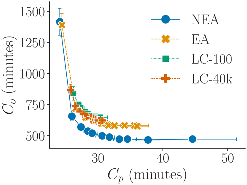
(a) Mumford1

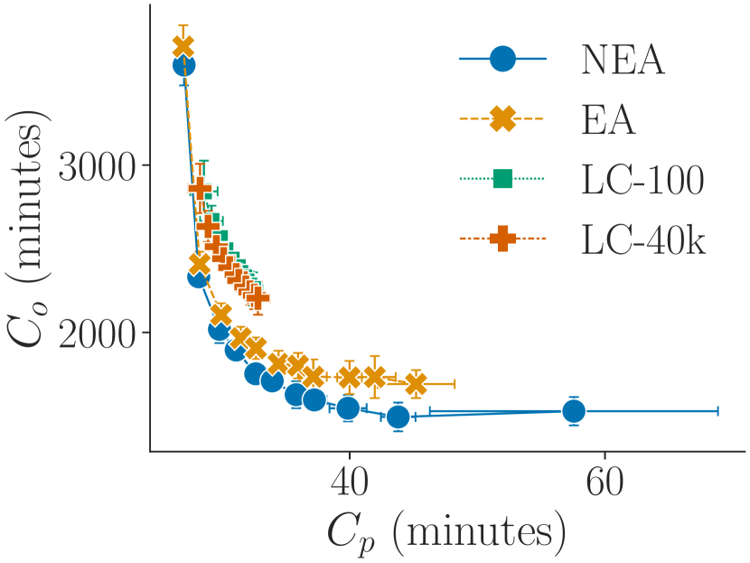
(b) Mumford2

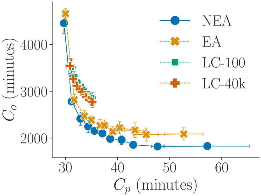
(c) Mumford3

Figure 3: Trade-offs between average trip time $C_{p}$ (on the x-axis) and total route time $C_{o}$ (on the y-axis), across values of $\alpha$ over the range $[0,1]$ in increments of $0.1$, from $\alpha=0.0$ at lower-right to $1.0$ at upper-left, for transit networks from LC-100, LC-40k, EA, and NEA. Each point shows the mean $C_{p}$ and $C_{o}$ over 10 random seeds for one value of $\alpha$, and bars around each point indicate one standard deviation on each axis. Lines linking pairs of points indicate that they represent consecutive $\alpha$ values. Lower values of $C_{o}$ and $C_{p}$ are better, so the down-and-leftward direction in each plot represents improvement.

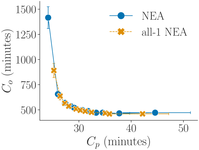
(a) Mumford1

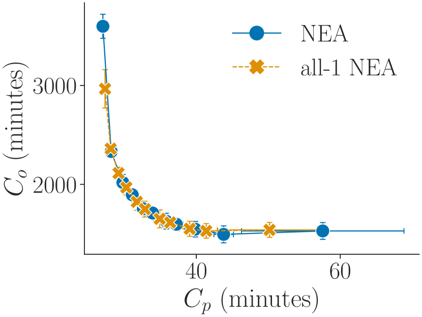
(b) Mumford2

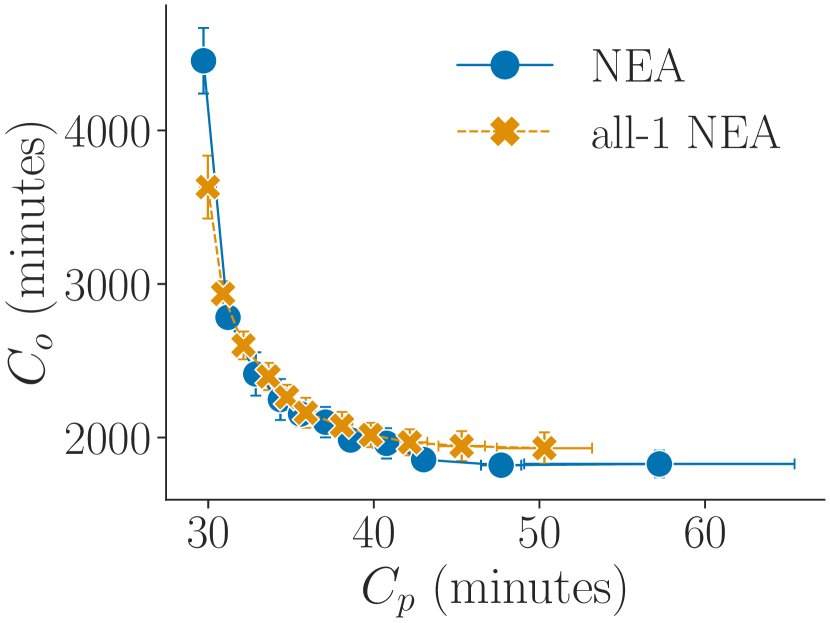
(c) Mumford3

Figure 4: Trade-offs between average trip time $C_{p}$ (on the x-axis) and total route time $C_{o}$ (on the y-axis) achieved by all-1 NEA, plotted along with NEA (repeated from Figure 3) for comparison.

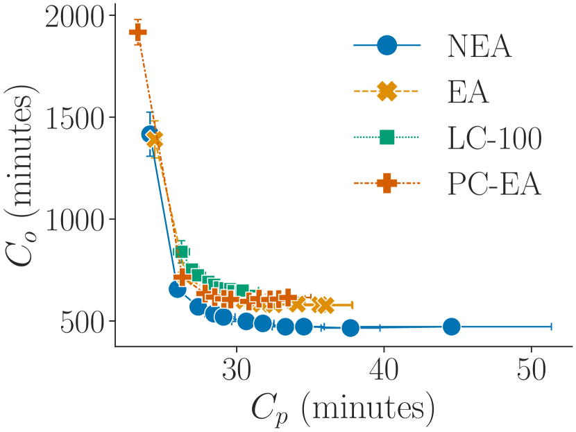
(a) Mumford1

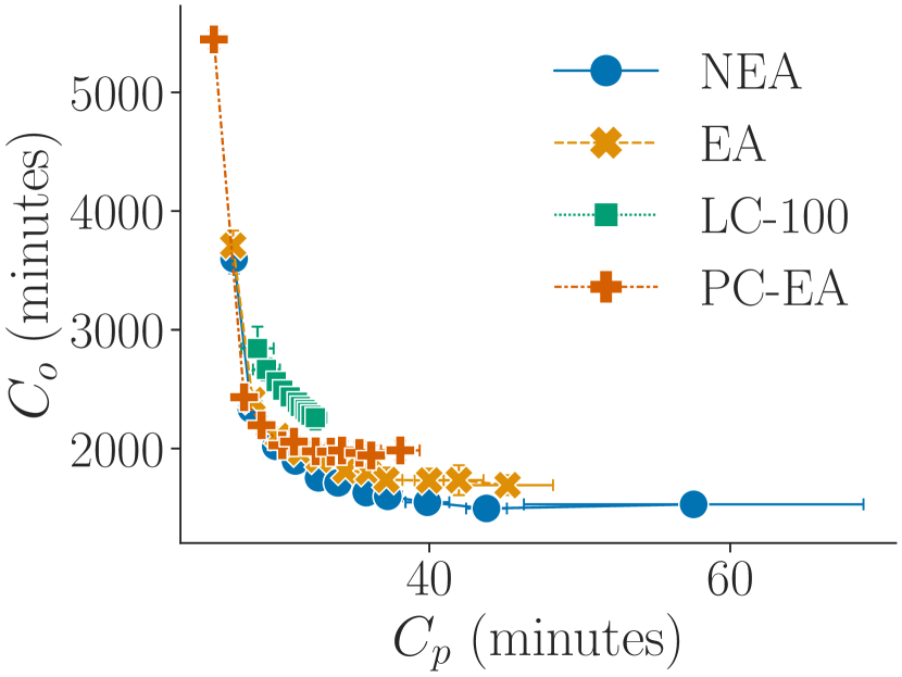
(b) Mumford2

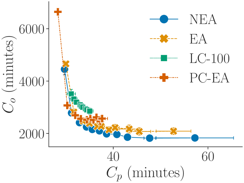
(c) Mumford3

Figure 5: Trade-offs between average trip time $C_{p}$ (on the x-axis) and total route time $C_{o}$ (on the y-axis) achieved by PC-EA, plotted along with LC-100, EA, and NEA (repeated from Figure 3) for comparison.

5.2 Ablation Studies

To better understand the contribution of various components of our method, we performed three sets of ablation studies. These were conducted over the three realistic Mumford cities (1, 2, and 3) and over eleven $\alpha$ values evenly spaced over the range $[0,1]$ in increments of 0.1.

5.2.1 Effect of number of samples

We note that over the course of the evolutionary algorithm, with our parameter settings $B=10,IT=400,E=10$, a total of $B\times IT\times E=40,000$ different transit networks are considered. By comparison, LC-100 only considers 100 networks. It could be that NEA’s superiority to LC-100 is only due to its considering more networks. To test this, we ran LC-40k, in which we sample $40,000$ networks from the learned-construction algorithm, and pick the lowest-cost network. Comparing LC-100 and LC-40k in Figure 3, we see that across all three cities and all values of $\alpha$, LC-40k performs very similarly to LC-100, improving on it only slightly in comparison with the larger improvements given by EA or NEA. From this we conclude that the number of networks considered is not on its own an important factor in EA’s and NEA’s performance: much more important is the evolutionary algorithm that guides the search of possible networks.

5.2.2 Contribution of type-2 mutator

We next considered the impact of the type-2 mutator heuristic on NEA. This low-level heuristic is the same between EA and NEA and is not a learned function. To understand how important it is to NEA’s performance, we ran “all-1 NEA”, a variant of NEA in which only the neural mutator is used, and not the type-2 mutator. The results are shown in Figure 4, along with the curve for NEA as in Figure 3, for comparison. It is clear that NEA and all-1 NEA perform very similarly in most scenarios. The differences are most notable at the extreme values of $\alpha$ (at either end of each curve), where we see that all-1 NEA underperforms NEA, achieving higher values of the relevant cost function component; but at intermediate $\alpha$ values on Mumford1 and Mumford2, NEA and all-1 NEA’s trip-time-versus-operating-cost curves overlap. It appears that the minor adjustments to existing routes made by the type-2 mutator are more important at extremes of $\alpha$, where the neural net policy has been pushed to the extremes of its behaviour.

On Mumford3, we observe that the curves do not overlap as cleanly; particularly for $\alpha\leq 0.5$, NEA seems to slightly outperform all-1 NEA. So the contribution of the type-2 mutator appears to grow as the city gets larger and more challenging. This may be because as the city gets larger, the space of possible routes grows larger, so the neural mutator’s changes get more dramatic in comparison with the single-node adjustments of the type-2 mutator. The type-2 mutator’s class of changes becomes more distinct from those of the neural mutator, possibly making it more important.

While the type-2 mutator’s contribution is small, it does help performance in some cases. We conclude that it is a useful component of the algorithm.

5.2.3 Importance of learned heuristics

We note that the type-1 mutator used in EA and the neural mutator used in NEA differ in the space of changes each is capable of making. The type-1 mutator can only add shortest paths as routes, while the neural mutator may compose multiple shortest paths into its new routes. It may be that this structural difference, as opposed to the quality of heuristics learned by the policy $\pi_{\theta}$, is part of NEA’s advantage over EA.

To test this conjecture, we ran a variant of NEA in which the learned policy $\pi_{\theta}$ is replaced by a policy $\pi_{\text{random}}$ that chooses actions uniformly at random:

$$\pi_{\text{random}}(a|s_{t})=\frac{1}{|\mathcal{A}_{t}|}\;\forall\;a\in\mathcal{A}_{t}$$

We call this variant the path-combining evolutionary algorithm (PC-EA). Since we wanted to gauge the performance of this variant in isolation from the learned policy, we did not use LC-100 with $\pi_{\theta}$ to generate the initial network $\mathcal{R}_{0}$. Instead, we used $\pi_{\text{random}}$ in LC-100 to generate $\mathcal{R}_{0}$ for PC-EA.

The results are shown in Figure 5, along with the same LC-100, EA, and NEA curves as in Figure 3. For most values of $\alpha$, PC-EA performs less well than both EA and NEA. But at the extreme of $\alpha=1.0$ it performs better than both NEA and EA, decreasing average trip time $C_{p}$ by between one and two minutes versus NEA on each city - an improvement of about 5% on Mumford1 and Mumford3 and about 3.5% on Mumford2.

PC-EA’s poor performance at low $\alpha$ makes sense: its ability to replace routes with composites of shortest paths biases it towards making longer routes, moreso than EA, and unlike $\pi_{\theta}$, $\pi_{\text{random}}$ cannot learn to prefer halting early in such cases. This is an advantage over EA at $\alpha=1.0$ but a disadvantage at $\alpha$ less than about $0.8$. It is interesting, though, that PC-EA outperforms NEA at $\alpha=1.0$, as these two share the same space of possible actions. We would expect that the neural net policy used in NEA should be able to learn to reach that performance of PC-EA simply by learning to choose actions uniformly at random. Yet somehow it fails to do so.

Nonetheless, NEA performs better overall than PC-EA, and so we leave the exploration of this mystery to future work. For now we merely note that composing shortest paths is a good heuristic for route construction at high $\alpha$, but is worse than simply choosing shortest paths at low $\alpha$; so the advantage of NEA comes primarily from what the policy $\pi_{\theta}$ learns during training.

5.3 Comparisons with prior work

While conducting the experiments of subsection 5.1, we observed that after 400 iterations the cost of NEA’s best-so-far network $\mathcal{R}_{\text{best}}$ was still decreasing from one iteration to the next. In order to make a fairer comparison with other methods from the literature on the Mandl and Mumford benchmarks, we performed a further set of experiments where we ran NEA with $IT=4,000$ instead of $400$, for the operator perspective ($\alpha=0.0$) and the passenger perspective ($\alpha=1.0$). In addition, because we observed better performance from PC-EA for $\alpha$ near $1.0$, we also ran PC-EA with $IT=4,000$ for $\alpha=1.0$, and we include these results in the comparison.

Table 3 and Table 4 present the results of these experiments on the Mandl and Mumford benchmarks, alongside results reported on these benchmarks in comparable recent work. As elsewhere, the results we report for NEA and PC-EA are averaged over ten runs with different random seeds; the same set of ten trained policies used in the experiments of subsection 5.1 and subsection 5.2 are used here in NEA. Results from other work are as reported in that work. In addition to the average trip time $C_{p}$ and total route time $C_{o}$, the tables present metrics of how many transfers between routes were required by the networks. These are labelled $d_{0}$, $d_{1}$, $d_{2}$, and $d_{un}$. $d_{i}$ with $i\in\{0,1,2\}$ is the percentage of all passenger trips that required $i$ transfers between routes; while $d_{un}$ is the percentage of trips that require more than 2 transfers ($d_{un}=100-(d_{0}+d_{1}+d_{2})$).

In these comparisons, we do not include results from Ahmed et al. (2019). While they reported results that set a new state of the art on these benchmarks, they do not provide the values used for the two parameters to their algorithm. In our earlier work Holliday and Dudek (2023), theirs was one of several methods we implemented in order to test our proposed initialization scheme. We discovered parameter values on our own that gave results comparable to other work up to 2019. But unfortunately, after much effort and correspondence with one of the authors of that work, we were unable to replicate their new state-of-the-art results. For this reason, we do not include their reported results here.

Before discussing these results, a brief word should be said about computation time. On a desktop computer with a 2.4 GHz Intel i9-12900F processor and an NVIDIA RTX 3090 graphics processing unit (used to accelerate our neural net computations), NEA takes about 3 hours for each run on Mumford3, the largest environment, while the PC-EA runs take about 2.5 hours. By comparison, John et al. (2014) and Hüsselmann et al. (2023) both use a variant of NSGA-II, a genetic algorithm, with a population of 200 networks, which in both cases takes more than two days to run on Mumford3. Hüsselmann et al. (2023)’s DBMOSA variant, meanwhile, takes 7 hours and 52 minutes to run on Mumford3. Kılıç and Gök (2014) report that their procedure takes eight hours just to construct the initial network for Mumford3, and don’t report the running time for the subsequent optimization.

These reported running times are not directly comparable as the experiments were not run on identical hardware, but the differences are broadly indicative of the differences in speed of these methods. The running times of these methods is mainly a function of the metaheuristic algorithm used, rather than the low-level heuristics used in the algorithm. Genetic algorithms like NSGA-II, with large populations as used in some of these methods, are very time-consuming because of the large number of networks they must modify and evaluate at each step. But their search of solution space is correspondingly more exhaustive than single-solution methods such as simulated annealing, or an evolutionary algorithm with a small population ($B=10$) as we use in our own experiments. It is therefore to be expected that they would achieve lower final costs in exchange for their greater run-time. We are interested here in the quality of the low-level heuristics we propose, rather than the metaheuristic algorithm, and this must be kept in mind as we discuss the results of this section.

City	Method	$C_{p}\downarrow$	$C_{o}\downarrow$	$d_{0}\uparrow$	$d_{1}$	$d_{2}$	$d_{un}\downarrow$
Mandl	Mumford (2013a)	10.27	221	95.38	4.56	0.06	0
	John et al. (2014)	10.25	212	-	-	-	-
	Kılıç and Gök (2014)	10.29	216	95.5	4.5	0	0
	Hüsselmann et al. (2023) DBMOSA	10.27	179	95.94	3.93	0.13	0
	Hüsselmann et al. (2023) NSGA-II	10.19	197	97.36	2.64	0	0
	NEA	10.42	185	92.49	7.24	0.27	0
	PC-EA	10.32	194	94.15	5.74	0.11	0
Mumford0	Mumford (2013a)	16.05	759	63.2	35.82	0.98	0
	John et al. (2014)	15.4	745	-	-	-	-
	Kılıç and Gök (2014)	14.99	707	69.73	30.03	0.24	0
	Hüsselmann et al. (2023) DBMOSA	15.48	431	65.5	34.5	0	0
	Hüsselmann et al. (2023) NSGA-II	14.34	635	86.94	13.06	0	0
	NEA	15.84	559	52.19	42.41	5.35	0.05
	PC-EA	14.96	722	63.21	36.36	0.43	0
Mumford1	Mumford (2013a)	24.79	2038	36.6	52.42	10.71	0.26
	John et al. (2014)	23.91	1861	-	-	-	-
	Kılıç and Gök (2014)	23.25	1956	45.1	49.08	5.76	0.06
	Hüsselmann et al. (2023) DBMOSA	22.31	1359	57.14	42.63	0.23	0
	Hüsselmann et al. (2023) NSGA-II	21.94	1851	62.11	37.84	0.05	0
	NEA	24.08	1414	33.58	45.44	18.51	2.47
	PC-EA	23.01	1924	39.57	49.66	10.46	0.32
Mumford2	Mumford (2013a)	28.65	5632	30.92	51.29	16.36	1.44
	John et al. (2014)	27.02	5461	-	-	-	-
	Kılıç and Gök (2014)	26.82	5027	33.88	57.18	8.77	0.17
	Hüsselmann et al. (2023) DBMOSA	25.65	3583	48.07	51.29	0.64	0
	Hüsselmann et al. (2023) NSGA-II	25.31	4171	52.56	47.33	0.11	0
	NEA	26.63	3973	32.42	48.89	17.48	1.21
	PC-EA	25.45	5536	41.18	52.96	5.84	0.02
Mumford3	Mumford (2013a)	31.44	6665	27.46	50.97	18.79	2.81
	John et al. (2014)	29.5	6320	-	-	-	-
	Kılıç and Gök (2014)	30.41	5834	27.56	53.25	17.51	1.68
	Hüsselmann et al. (2023) DBMOSA	28.22	4060	45.07	54.37	0.56	0
	Hüsselmann et al. (2023) NSGA-II	28.03	5018	48.71	51.1	0.19	0
	NEA	29.27	5155	30.36	51.01	17.43	1.2
	PC-EA	28.09	6830	38.6	57.02	4.35	0.03

Table 3: Passenger-perspective results. $C_{p}$ is the average passenger trip time. $C_{o}$ is the total route time. $d_{i}$ is the percentage of trips satisfied with number of transfers $i$, while $d_{un}$ is the percentage of trips satsified with 3 or more transfers. Arrows next to each quantity indicate which of increase or decrease is desirable. Bolded values in $C_{p}$, $d_{0}$, and $d_{un}$ columns are the best on that environment.

5.3.1 Passenger-perspective results

Table 3 shows the passenger perspective results alongside results from other work. On each city except Mumford1, the NSGA-II variant of Hüsselmann et al. (2023) has the best final performance; it is also among the most time-consuming of the algorithms reported on here. PC-EA and NEA both perform poorly on the smallest two cities, Mandl and Mumford0, but their relative performance improves as the size of the city increases. On both Mumford2 and Mumford3, PC-EA’s performance is very close to that of Hüsselmann et al. (2023)’s NSGA-II, and better than all other methods listed, despite the relatively under-powered metaheuristic that drives it.

PC-EA also outperforms Hüsselmann et al. (2023)’s DBMOSA, which uses the same low-level heuristics as their NSGA-II with a faster but less-exhaustive metaheuristic. That PC-EA exceeds DBMOSA’s performance on Mumford2 and Mumford3 is evidence that the low-level heuristics used in PC-EA are better for the passenger perspective than those proposed by Hüsselmann et al. (2023). This is especially the case given that DBMOSA is still a more sophisticated metaheuristic algorithm than ours, with ten different low-level heuristics and a hyper-heuristic that adapts the rate at which each low-level heuristic is applied over the run.

NEA does not perform as well as PC-EA on the passenger perspective (aligning with what we observed in subsection 5.2), but still shows good performance on Mumford2 and 3, outperforming all of these methods that were published prior to 2022.

5.3.2 Operator-perspective results

Table 4 shows the operator-perspective results alongside results from other work. Kılıç and Gök (2014) do not report results for the operator perspective and as such we do not include their work in Table 4. Similarly to the passenger-perspective results, our methods underperform on the smallest cities (Mandl and Mumford0) but perform well on larger ones. Strikingly, NEA achieves the lowest value of total route time $C_{o}$ out of all methods on Mumford1, 2, and 3, improving even on Hüsselmann et al. (2023)’s NSGA-II. Evidently, the learned policy functions very well as a low-level heuristic at low values of $\alpha$, where the premium is on keeping routes short.

City	Method	$C_{o}\downarrow$	$C_{p}$	$d_{0}\uparrow$	$d_{1}$	$d_{2}$	$d_{un}\downarrow$
Mandl	Mumford (2013a)	63	15.13	70.91	25.5	2.95	0.64
	John et al. (2014)	63	13.48	-	-	-	-
	Hüsselmann et al. (2023) DBMOSA	63	13.55	70.99	24.44	4.00	0.58
	Hüsselmann et al. (2023) NSGA-II	63	13.49	71.18	25.21	2.97	0.64
	NEA	67	14.19	56.80	32.02	10.66	0.53
Mumford0	Mumford (2013a)	111	32.4	18.42	23.4	20.78	37.40
	John et al. (2014)	95	32.78	-	-	-	-
	Hüsselmann et al. (2023) DBMOSA	98	27.61	22.39	31.27	18.82	27.51
	Hüsselmann et al. (2023) NSGA-II	94	27.17	24.71	38.31	26.77	10.22
	NEA	116	29.47	14.83	31.74	29.12	24.31
Mumford1	Mumford (2013a)	568	34.69	16.53	29.06	29.93	24.66
	John et al. (2014)	462	39.98	-	-	-	-
	Hüsselmann et al. (2023) DBMOSA	511	26.48	25.17	59.33	14.54	0.96
	Hüsselmann et al. (2023) NSGA-II	465	31.26	19.70	42.09	33.87	4.33
	NEA	448	43.22	14.15	22.44	23.53	39.87
Mumford2	Mumford (2013a)	2244	36.54	13.76	27.69	29.53	29.02
	John et al. (2014)	1875	32.33	-	-	-	-
	Hüsselmann et al. (2023) DBMOSA	1979	29.91	22.77	58.65	18.01	0.57
	Hüsselmann et al. (2023) NSGA-II	1545	37.52	13.48	36.79	34.33	15.39
	NEA	1446	62.27	8.14	14.60	16.65	60.60
Mumford3	Mumford (2013a)	2830	36.92	16.71	33.69	33.69	20.42
	John et al. (2014)	2301	36.12	-	-	-	-
	Hüsselmann et al. (2023) DBMOSA	2682	32.33	23.55	58.05	17.18	1.23
	Hüsselmann et al. (2023) NSGA-II	2043	35.97	15.02	48.66	31.83	4.49
	NEA	1788	56.04	8.74	15.81	19.86	55.58

Table 4: Operator perspective results. $C_{p}$ is the average passenger trip time. $C_{o}$ is the total route time. $d_{i}$ is the percentage of trips satisfied with number of transfers $i$, while $d_{un}$ is the percentage of trips satsified with 3 or more transfers. Arrows next to each quantity indicate which of increase or decrease is desirable. Bolded values in $C_{o}$, $d_{0}$ and $d_{un}$ columns are the best on that environment.

The metrics $d_{0}$ to $d_{un}$ reveal that both PC-EA and NEA favour higher numbers of transfers relative to most of the other methods, particularly Hüsselmann et al. (2023). This is true for both the passenger and operator perspectives. For the operator perspective, this matches our intuitions: shorter routes will deliver fewer passengers directly to their destinations. But we were surprised to observe this in the passenger perspective case as well.

Compared to Hüsselmann et al. (2023)’s DBMOSA, PC-EA achieves lower average trip time $C_{p}$ on Mumford2 and Mumford3 for the passenger perspective, despite the fact that it requires more passenger trips to make 1 and 2 transfers. Still, PC-EA does give fewer transfers overall than NEA, which matches our intuition that fewer transfers should result in lower average trip time $C_{p}$. It seems that the process of compositing shortest paths to form routes biases those routes towards directness and efficiency, to a degree that outweighs the cost imposed by having more transfers. Each transfer is less impactful on riders if the routes they’re transferring between are more direct.

Meanwhile, since both the learned heuristic of NEA and the unlearned heuristic of PC-EA suffer from high transfer counts, it seems the difference between these and the other results from the literature may be a result of the evolutionary algorithm itself. At any rate, these results are not out of line with those of Mumford (2013a) and Kılıç and Gök (2014) on the largest cities, so we do not consider this a major strike against our learned heuristics. Indeed, we expect that these results could be improved by explicitly including $d_{0}$ in the reward function used to train the policy $\pi_{\theta}$, and this would reduce the number of transfers required by NEA’s networks.

6 LAVAL EXPERIMENTS

To assess our method in a realistic problem instance, we applied it to data from the city of Laval in Quebec, Canada. Laval is a suburb of the major Canadian city of Montreal. As of the 2021 census, it had a total population of 429,555 (Statistics Canada, 2023). Public transit in Laval is provided primarily by the bus network of the Société de Transport de Laval; additionally, one line of the Montreal underground metro system has three stops in Laval.

6.1 Representing Laval

To apply our learned policy $\pi_{\theta}$ to Laval, we first had to assemble a realistic city graph $\mathcal{C}=(\mathcal{N},\mathcal{E}_{s},D)$ representing Laval from the data sources that were available to us. Our model of the city of Laval is based on several sources: geographic data on census dissemination areas for 2021 from Statistics Canada (Statistics Canada, 2021), a GIS representation of the road network of Laval provided to us by the Société de Transport de Laval, an OD dataset (Agence métropolitaine de transport, 2013) provided by Quebec’s Agence Métropolitaine de Transport, and publicly-available GTFS data from 2013 (STL, ) that describes Laval’s existing transit system.

6.1.1 Street graph

The street graph $(\mathcal{N},\mathcal{E}_{s})$ was derived from the 2021 census data by taking the centroid of each CDA within Laval to be a node in $\mathcal{N}$, and adding a street edge $(i,j,t_{ij})$ for node pair $(i,j)$ if their corresponding CDAs shared a border. To compute drive times $t_{ij}$, we found all points in the road network within the CDAs of $i$ and $j$, computed the shortest-path driving time over the road network from each of $i$’s road-network points to each of $j$’s, and set $t^{\prime}_{ij}$ as the median of these driving times. We did this so that $t^{\prime}_{ij}$ would reflect the real drive times given the existing road network. By this approach, $t^{\prime}_{ij}\neq t^{\prime}_{ji}$ in general, but as our method treats cities as undirected graphs, it expects that $t_{ij}=t_{ji}\;\forall\;i,j\in\mathcal{N}$. To enforce this, as a final step we set:

$$t_{ij}=t_{ji}=\max(t^{\prime}_{ij},t^{\prime}_{ji})\;\forall\;i,j\in\mathcal{N}$$ (10)

6.1.2 Existing transit

The existing transit network in Laval has 43 bus routes that operate during morning rush hour from 7 to 9 AM. To compare networks from our algorithm to the this network, we had to translate it to a network that runs over $(\mathcal{N},\mathcal{E}_{s})$ as defined in subsection 6.1.1. To do this, we mapped each stop on an existing bus route to a node in $\mathcal{N}$ based on which CDA contains the stop. We will refer to this translated transit system as the STL network, after the city’s transit agency, the Société de Transport de Laval.

The numbers of stops on the routes in the STL network range from 2 to 52. To ensure a fair comparison, we set $MIN=2$ and $MAX=52$ when running our algorithm. Unlike the routes in our algorithm’s networks, many of STL’s routes are not symmetric (that is, they follow a different path in each direction between terminals), and several are unidirectional (they go only one way between terminals). We maintained the constraints of symmetry and bidirectionality on our own algorithm, but did not enforce them upon the STL network. The only modification we made is that when reporting total route time $C_{o}$ in this section, we calculated it for bidirectional routes by summing the travel times of both directions, instead of just one direction as in the preceding sections.

In addition, there is an underground metro line, the Montreal Orange Line, which has three stops in Laval. As with the existing bus lines, we mapped these three stops to their containing CDAs and treat them as forming an additional route. We added this metro route to both the STL network and the networks $\mathcal{R}$ produced by our algorithm when evaluating them, to reflect that unlike the bus routes, it is not feasible to change the metro line and so it represents a constant of the city.

6.1.3 Demand matrix

Finally we assembled the demand matrix $D$ from the OD dataset. The entries in the OD dataset correspond to trips reported by residents of Laval who were surveyed about their recent travel behaviour. Each entry has (lat,lon) coordinates $l_{o}$ and $l_{d}$ for the trip’s approximate origin and destination, as well as an “expansion factor” $e$ giving the estimated number of actual trips corresponding to that surveyed trip. It also indicates the mode of travel, such as car, bicycle, or public transit, that was used to make the trip.

Many entries in the OD dataset refer to trips that begin or end in Montreal. For our purposes, we “redirected” all trips made by public transit that enter or leave Laval to one of several “crossover points” that we defined. These crossover points are the locations of the three Orange Line metro stations in Laval, and the locations of the last or first stop in Laval of each existing bus route that goes between Laval and Montreal.

For each trip between Laval and Montreal, we identified the crossover point that has the shortest distance to either of $l_{o}$ or $l_{d}$, and overwrote the Montreal end-point of the trip by this crossover point. This process was automated with a simple computer script. The idea is that if the Laval end of the trip is close to a transit stop that provides access to Montreal, the rider will choose to cross over to the Montreal transit system as soon as possible, as most locations in Montreal will be easier to access once in the Montreal transit system. Trips that go between Laval and Montreal by means other than public transit were not included in $D$, as we judge that most such trips cannot be induced to switch modes to transit.

Having done this remapping, we initialized $D$ with all entries set to 0. Then for each entry in the OD dataset, we found the CDAs that contain $l_{o}$ and $l_{d}$, associated them with the matching nodes $i$ and $j$ in $\mathcal{N}$, and updated $D_{ij}\leftarrow D_{ij}+e$. $D$ then had the estimated demand between every pair of CDAs. To enforce symmetric demand, we then assigned $D_{ij}\leftarrow\max(D_{ij},D_{ji})\;\forall\;i,j\in\mathcal{N}$. The resulting demand matrix $D$ contains 548,159 trips, of which 63,104 are trips between Laval and Montreal that we redirected.

We then applied a final filtering step. The STL network does not provide a path between all node-pairs $i,j$ for which $D_{ij}>0$, and so it violates constraint 1 of section 3. This is because $D$ at this point includes all trips that were made within Laval by any mode of transport, including to and from areas that are not served by the STL network. These areas may be unserved because they are populated by car owners unlikely to use transit if it were available. To ensure a fair comparison between the STL network and our algorithm’s networks, we set to 0 all entries of $D$ for which the STL network does not provide a path. We expected this to cause our system to output transit networks that are “closer” to the existing transit network, in that they satisfy the same travel demand as before. This should reduce the scope of the changes required to go from the existing network to a new one proposed by our system.

Table 5 contains the statistics of, and parameters used for, the Laval scenario.

Table 5: Statistics and parameters of the Laval scenario

# nodes $n$	# street edges $|\mathcal{E}_{s}|$	# demand trips	# routes $S$	$MIN$	$MAX$	Area (km2)
632	4,544	548,159	43	2	52	520.1

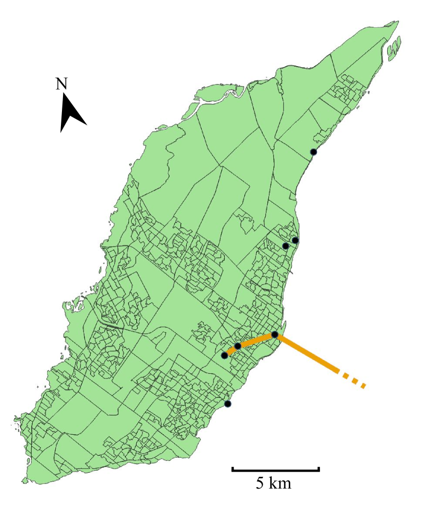
(a) Census dissemination areas

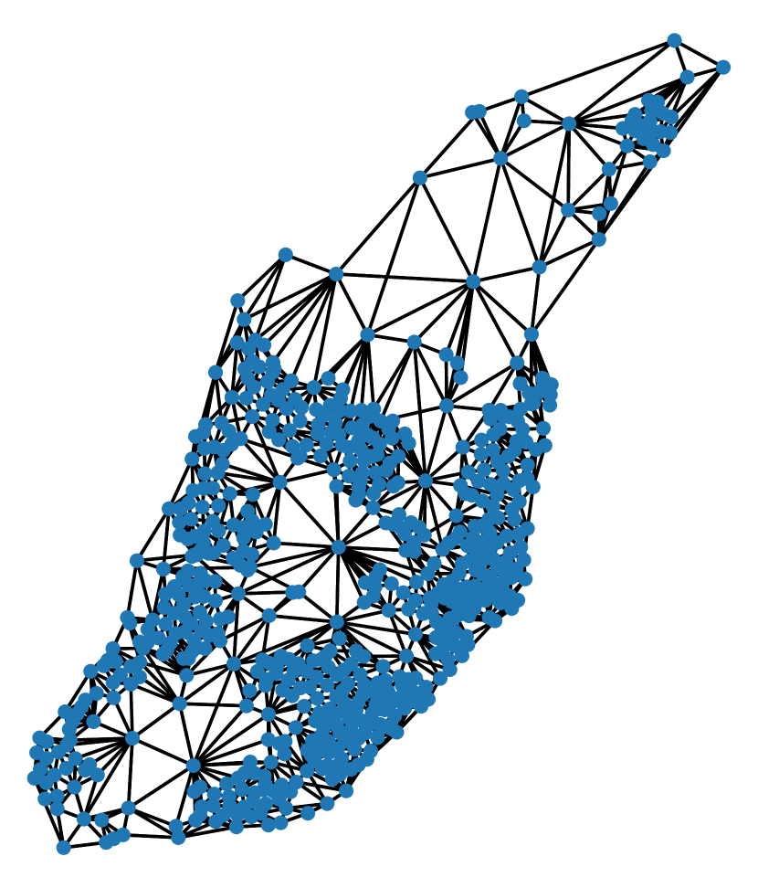
(b) Street graph

Figure 6: 6(a) shows a map of the census dissemination areas of the city of Laval, with “crossover points” used to remap inter-city demands shown as black circles, and the Montreal Metro Orange Line shown in orange. 6(b) shows the street graph constructed from these dissemination areas.

6.2 Enforcing constraint satisfaction

In the experiments on the Mandl and Mumford benchmark cities described in section 5, the EA and NEA algorithms never produced networks violated any of the constraints on networks outlined in section 3. However, Laval’s city graph, with 632 nodes, is considerably larger than even the largest Mumford city, which has only 127 nodes. In our initial experiments on Laval, we found that both EA and NEA consistently produced networks that violated constraint 1, providing no transit path for some node pairs $(i,j)$ for which $D_{ij}>0$.

To remedy this, we modified the MDP described in subsection 3.1 to enforce reduction of unsatisfied demand. Let $c_{1}(\mathcal{C},\mathcal{R})$ be the number of node-pairs $i,j$ with $D_{ij}>0$ for which network $\mathcal{R}$ provides no transit path, and let $\mathcal{R}^{\prime}_{t}=\mathcal{R}_{t}\cup\{r_{t}\}$, the network formed from the finished routes and the in-progress route $r_{t}$. We applied the following changes to the action space $\mathcal{A}_{t}$ whenever $c_{1}(\mathcal{R}_{t})>0$:

• When the timestep $t$ is even and $\mathcal{A}_{t}$ would otherwise be $\{\textup{continue},\textup{halt}\}$, the halt action is removed from $\mathcal{A}_{t}$. This means that if $c_{1}(\mathcal{C},\mathcal{R}^{\prime}_{t})>0$, the current route must be extended if it is possible to do so without violating another constraint.

• When $t$ is odd, if $\mathcal{A}_{t}$ contains any paths that would reduce $c_{1}(\mathcal{C},\mathcal{R}^{\prime}_{t})$ if added to $r_{t}$, then all paths that would not reduce $c_{1}(\mathcal{C},\mathcal{R}^{\prime}_{t})$ are removed from $\mathcal{A}_{t}$. This means that if it is possible to connect some unconnected trips by extending $r_{t}$, then not doing so is forbidden.

With these changes to the MDP, we found that both LC-100 and NEA produced networks that connected all desired passenger trips, with no constraint violations - even when the policy $\pi_{\theta}$ was trained without these changes. The results reported in this section are obtained using this variant of the MDP.

6.3 Experiments

We performed experiments evaluating both the NEA and PC-EA algorithms on the Laval city graph. Three sets of experiments were performed with different $\alpha$ values representing different perspectives: the operator perspective ($\alpha=0.0$), the passenger perspective ($\alpha=1.0$), and a balanced perspective ($\alpha=0.5$). As in section 5, we perform ten runs of each experiment with ten different random seeds and ten different learned policies $\pi_{\theta}$, and report statistics over these ten runs; the same per-seed parameters $\theta$ are used as in the experiments of section 5. We also run the STL network on the Laval city graph $\mathcal{C}$ in the same way that we run the networks from our other algorithms to measure their performance, but since the STL network is a single, pre-determined network that does not depend on $\alpha$, we run it only once.

Some trial runs we performed with $IT=4,000$ showed that the network cost stopped decreasing after $2,700$ iterations, so to save time we ran our final NEA and PC-EA experiments on Laval with $IT=3,000$. The other parameters of the algorithm were the same as in the Mumford experiments: $B=10$, $E=10$, and transfer penalty $p_{T}=300$s.

6.3.1 Results

The results of the Laval experiments are shown in Table 6. The results for the initial networks produced by LC-100 are presented as well, to show how much improvement the NEA makes over its initial networks. Figure 7 highlights the trade-offs each method achieves between average trip time $C_{p}$ and total route time $C_{o}$, and how they compare to the STL network.

$\alpha$	Method	$C_{p}\downarrow$	$C_{o}\downarrow$	$d_{0}\uparrow$	$d_{1}$	$d_{2}$	$d_{un}\downarrow$
N/A	STL	124.61	23954	14.48	22.8	20.88	41.83
	LC-100	88.83 $\pm$ 11.53	21893 $\pm$ 5096	14.19 $\pm$ 1.28	23.45 $\pm$ 3.97	23.58 $\pm$ 2.71	38.78 $\pm$ 7.52
0.0	NEA	96.65 $\pm$ 12.10	19624 $\pm$ 2455	14.22 $\pm$ 0.97	23.57 $\pm$ 3.67	23.63 $\pm$ 2.41	38.57 $\pm$ 6.39
	PC-EA	67.67 $\pm$ 1.37	31907 $\pm$ 1295	16.56 $\pm$ 0.65	32.94 $\pm$ 1.09	29.06 $\pm$ 0.92	21.44 $\pm$ 2.04
	LC-100	79.32 $\pm$ 8.27	24124 $\pm$ 7736	14.88 $\pm$ 1.98	24.87 $\pm$ 5.22	24.53 $\pm$ 1.85	35.72 $\pm$ 8.49
0.5	NEA	82.55 $\pm$ 7.11	20978 $\pm$ 3424	14.40 $\pm$ 1.35	24.44 $\pm$ 4.16	24.76 $\pm$ 2.17	36.41 $\pm$ 7.00
	PC-EA	67.40 $\pm$ 1.23	31784 $\pm$ 1171	16.33 $\pm$ 0.62	33.35 $\pm$ 0.75	28.99 $\pm$ 0.75	21.33 $\pm$ 1.21
	LC-100	66.49 $\pm$ 4.12	32270 $\pm$ 8551	16.35 $\pm$ 1.89	29.77 $\pm$ 3.30	26.04 $\pm$ 2.15	27.85 $\pm$ 5.37
1.0	NEA	59.23 $\pm$ 0.86	45382 $\pm$ 2627	20.99 $\pm$ 0.91	34.48 $\pm$ 2.48	26.71 $\pm$ 0.52	17.82 $\pm$ 3.30
	PC-EA	57.42 $\pm$ 0.41	49016 $\pm$ 822	22.89 $\pm$ 0.60	39.39 $\pm$ 0.75	26.33 $\pm$ 0.72	11.38 $\pm$ 0.93

Table 6: Performance of networks from LC-100, NEA, and PC-EA at three $\alpha$ values, as well as the STL network. Bolded values are best for the corresponding $\alpha$. $C_{p}$ is the average passenger trip time. $C_{o}$ is the total route time. $d_{i}$ is the percentage of trips satisfied with number of transfers $i$, while $d_{un}$ is the percentage of trips satsified with 3 or more transfers. All values are averaged over ten random seeds, with one standard deviation following “$\pm$”, except for those in the STL row.

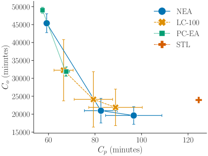
Figure 7: Average trip time $C_{p}$ versus total route time $C_{o}$ achieved by LC-100, NEA, and PC-EA, for $\alpha=0.0$ (bottom-right), 0.5 (middle), and 1.0 (top-left), as well as for the STL network itself (independent of $\alpha$). Except for STL, each point is a mean value over 10 random seeds, and bars show one standard deviation. Note that PC-EA’s $\alpha=0.0$ and 0.5 have nearly identical values (as shown in Table 6), so the corresponding points are stacked in this figure and appear as one point.

We see that for each value of $\alpha$, NEA’s network outperforms the STL network: it achieves 54% lower $C_{p}$ at $\alpha=1.0$, 18% lower $C_{o}$ at $\alpha=0.0$, and at $\alpha=0.5$, 34% lower $C_{p}$ and 12% lower $C_{o}$. At both $\alpha=0.0$ and $\alpha=0.5$, NEA strictly dominates both lower $C_{p}$ and lower $C_{o}$ than the existing transit system.

Comparing NEA’s results to LC-100, we see that at $\alpha=0.0$, NEA decreases $C_{o}$ and increases $C_{p}$ relative to LC-100; and for $\alpha=1.0$, the reverse is true. In both cases, NEA improves over the initial network on the objective being optimized, at the cost of the other, as we would expect. In the balanced case ($\alpha=0.5$), we see that NEA decreases $C_{o}$ by 13% while increasing $C_{p}$ by 4%. This matches what we observed in Figure 3, as discussed in subsection 5.1.

Looking at the transfer percentages $d_{0}$, $d_{1}$, $d_{2}$, and $d_{un}$, we see that as $\alpha$ increases, the overall number of transfers shrinks, with $d_{1}$ growing and $d_{un}$ shrinking. This is as expected, since fewer transfers usually means shorter passenger travel times. By the same token, PC-EA performs best on these metrics, as it does on average trip time $C_{p}$. Notably though, at $\alpha=0.0$ NEA’s $d_{0}$, $d_{1}$, and $d_{2}$ are only slightly worse than the STL network’s - the largest increase is in $d_{2}$, by 13% of STL’s value - while $d_{un}$ is less than the STL network’s, meaning that NEA’s output networks let more passengers reach their destination in 2 or fewer transfers than the STL network. In fact, the very small decrease in $d_{0}$ implies that the larger increases in $d_{1}$ and $d_{2}$ mostly come from trips that were in $d_{un}$ in the STL network; NEA has thus decreased the average number of transfers. This is a significant improvement, given that at $\alpha=0.0$ the algorithm is unconcerned with minimizing passenger travel time.

At $\alpha=0.5$, NEA’s $d_{un}$ decreases further and $d_{0}$, $d_{1}$, and $d_{2}$ correspondingly increase further. Then from $\alpha=0.5$ to $1.0$, NEA’s $d_{un}$ drops by more than half, and its $d_{0}$, $d_{1}$, and $d_{2}$ are all markedly increased, especially $d_{0}$ which is 31% greater than STL’s $d_{0}$. NEA improves on the STL network by a considerable margin at all three $\alpha$ values, even though PC-EA outperforms NEA at $\alpha=1.0$.

The likely aim of Laval’s transit agency is to reduce costs while improving service quality, or at least not harming it too much. The “balanced” case, where $\alpha=0.5$, is most relevant to that aim. In this balanced case, we find that NEA proposes networks that reduce total route time by 13% versus the existing STL transit network. Some simple calculations can help understand the savings this represents. The approximate cost of operating one of Laval’s buses is 200 Canadian dollars (CAD) per hour. Suppose that each route has the same headway (time between bus arrivals) $H$. Then, the number of buses $N_{r}$ required by route $r$ is the ceiling of the route’s driving time $\tau_{r}$ divided by the headway, $\left\lceil\frac{\tau_{r}}{H}\right\rceil$. The total number of buses $N_{\mathcal{R}}$ required for a transit network $\mathcal{R}$ is then:

$$N_{\mathcal{R}}=\sum_{r\in\mathcal{R}}N_{r}\approx\frac{1}{H}\sum_{r\in\mathcal{R}}\tau_{r}=\frac{C_{o}}{H}$$

The total cost of the system is 200 CAD$\times N_{\mathcal{R}}$. Assuming a headway of 15 minutes on all routes, that gives a per-hour operating cost of 319,387 CAD for the STL network, while the average operating cost of networks from NEA with $\alpha=0.5$ is 279,707 CAD. So, under these simplifying assumptions, NEA could save the Laval transit agency on the order of 40,000 CAD per hour - savings of more than 12% of costs. This is only a rough estimate: in practice, headways differ between routes, and there may be additional costs involved in altering the routes from the current system, such as from moving or building bus stops. But it shows that NEA, and neural heuristics more broadly, may offer practical savings to transit agencies.

In addition, NEA’s balanced-case networks reduce the average passenger trip time by 34% versus the STL network, and reduce the number of transfers that passengers have to make, especially reducing the percentage of trips that require three or more transfers from 41.83% to 36.41%. Trips requiring three or more transfers are widely regarded as being so unattractive that riders will not make them (but note that these trips are still included in the calculation of $C_{p}$). So NEA’s networks may even increase overall transit ridership. This not only makes the system more useful to the city’s residents, but also increases the agency’s revenue from fares.

We also note that PC-EA achieves lower average trip time $C_{p}$ than both STL and NEA for all three $\alpha$ values, but at the cost of worsening total route time $C_{o}$ versus STL in each case. Furthermore, at $\alpha=1.0$ where we disregard $C_{o}$, it achieves only 3% lower $C_{p}$ than NEA. This supports our conclusions in subsection 5.2.3 and subsection 5.3 that the learned heuristics of the neural net policies $\pi_{\theta}$ are the main driver of NEA’s performance, rather than simply the process of assembling routes from shortest paths.

In these experiments, the nodes of the graph represent census dissemination areas instead of existing bus stops. In order to be used in reality, the proposed routes would need to be fitted to the existing locations of bus stops in the CDAs, likely making multiple stops within each CDAs. To minimize the cost of the network redesign, it would be necessary to keep stops at most or all stop locations that have shelters, as constructing or moving these may cost tens of thousands of dollars, while stops with only a signpost at their locations can be moved at the cost of only a few thousand dollars. An algorithm for translating our census-level routes to real-stop-level routes, in a way that minimizes cost, is an important next step for making this work applicable. We leave this for future work.

7 CONCLUSIONS

The choice of low-level heuristics has a major impact on the effectiveness of a metaheuristic algorithm, and our results show that using deep reinforcement learning to learn heuristics can offer substantial benefits when used alongside human-engineered heuristics. They also show that learned heuristics may be useful in complex real-world transit planning scenarios. They can improve on an existing transit system in multiple dimensions, in a way sensitive to the planner’s preference over these dimensions, and so may enable transit agencies to offer better service at reduced cost.

Our heuristic-learning method has several limitations. One is that the construction MDP on which our neural net policies are trained differs from the evolutionary algorithm - an improvement process - in which it is deployed. Another is that it learns just one type of heuristic, that for constructing a route from shortest paths, though we note that the neural net may be learning multiple distinct heuristics for how to do this under different circumstances. Natural next steps would be to learn a more diverse set of heuristics, perhaps including route-lengthening and -shortening operators, and to train our neural net policies directly in the context of an improvement process, which may yield learned heuristics that are better-suited to that process.

A remaining question is why the random path-combining heuristic used in the PC-EA experiments outperforms the learned heuristic in the extreme of the passenger perspective. As noted in subsection 5.2.3, in principle the neural net should be able to learn whatever policy the random path-combiner is enacting: in the limit, it could learn to give the same probability to all actions when $\alpha=1.0$. We wish to explore in more depth why this does not occur, and whether changes to the policy architecture or learning algorithm might allow the learned heuristic’s performance to match or exceed that of the random policy.

The evolutionary algorithm in which we use our learned heuristic was chosen for its speed and simplicity, which aided in implementation and rapid experimentation. But as noted in subsection 4.2, other more costly state-of-the-art algorithms, like NSGA-II, may allow still better performance to be gained from learned heuristics. Future work should attempt to use learned heuristics like ours in more varied metaheuristic algorithms.

Another promising place where machine learning can be applied is to learn hyper-heuristics for a metaheuristic algorithm. A typical hyper-heuristic, as used by Ahmed et al. (2019) and Hüsselmann et al. (2023), adapts the probability of using each low-level heuristic based on its performance, while the algorithm is running. It would be interesting to train a neural net policy to act as a hyper-heuristic to select among low-level heuristics, given details about the scenario and previous steps taken during the algorithm.

Our aim in this paper was to show whether learned heuristics can be used in a lightweight metaheuristic algorithm to improve its performance. Our results show that they can, and in fact that they give performance competitive with, and in some cases better than, state-of-the-art algorithms using human-engineered heuristics. This is compelling evidence that they may help transit agencies substantially reduce operating costs while delivering better service to riders in real-world scenarios.

Appendix A Neural Net Architecture

In this appendix, we give a detailed description of the architecture of the neural net used in our GNN policy $\pi_{\theta}$.

A.1 Input Features

The policy net operates on three inputs: an $n\times 4$ matrix of node feature vectors $X$, an $n\times n\times 13$ tensor of edge features $E$, and a global state vector $\mathbf{s}$.

A node feature $x_{i}$ is composed of the $(x,y)$ coordinates of the node and its in-degree and out-degree in the street graph.

An edge feature $\mathbf{e}_{ij}$ is composed of the following elements:

• $D_{ij}$, the demand between the nodes

• $s_{ij}=1$ if $(i,j,\tau_{ij})\in\mathcal{E}_{s}$, $0$ otherwise

• $\tau_{ij}$ if $s_{ij}=1$, $0$ otherwise

• $c_{ij}=1$ if $\mathcal{R}$ links $i$ to $j$, $0$ otherwise

• $c_{0ij}=1$ if $j$ can be reached from $i$ over $\mathcal{R}$ with no transfers, $0$ otherwise

• $c_{1ij}=1$ if one transfer is needed to reach $j$ from $i$ over $\mathcal{R}$, $0$ otherwise

• $c_{2ij}=1$ if two transfers are needed to reach $j$ from $i$ over $\mathcal{R}$, $0$ otherwise

• $\textup{self}=1$ if $i=j$, $0$ otherwise

• $\tau_{\mathcal{R}ij}$ if $c_{ij}=1$, $0$ otherwise

• $\tau_{rij}$ if $c_{0ij}=1$ where $r$ the route that provides the shortest direct trip between $i$ and $j$, $0$ otherwise

• $T_{ij}$, the shortest-path driving time between the nodes

• $\alpha$ and $1-\alpha$, the weights of the two components of the cost function $C$

The global state vector $\mathbf{s}$ is composed of:

• Average passenger trip time given current route set, $C_{p}(\mathcal{C},\mathcal{R})$

• Total route time given current route set, $C_{o}(\mathcal{C},\mathcal{R})$

• number of routes planned so far, $|\mathcal{R}|$

• number of routes left to plan, $S-|\mathcal{R}|$

• fraction of node pairs with demand $d_{ij}>0$ that are not connected by $\mathcal{R}$

• $\alpha$ and $1-\alpha$, the weights of the two components of the cost function $C$

Note that $\alpha$ and $1-\alpha$ are included in both $\mathbf{s}$ and $\mathbf{e}_{ij}$.

A.2 Policy Network Architecture

The policy $\pi_{\theta}$ is a neural net with three components: a GAT “backbone”, a halting module $\textup{NN}_{halt}$, and an extension module $\textup{NN}_{ext}$. The halting and extension modules both operate on the outputs from the GNN. All nonlinearities are ReLU functions. A common embedding dimension of $d_{\text{embed}}=64$ is used throughout; unless otherwise specified, each component of the system outputs vectors of this dimension.

A.2.1 Backbone network

The backbone is a graph attention net composed of five GATv2(Brody et al., 2021) multi-head graph attention layers separated by ReLU nonlinearities. 4 heads are used in each multi-head attention layer. The network takes as input the node feature collection $X$ and the edge features $E$, and the final layer outputs a collection of node embeddings $Y=\{\mathbf{y}_{i}\;\forall i\in\mathcal{N}\}$. These node embeddings are used by the two policy heads to compute action probabilities.

A.2.2 Halting module

$\textup{NN}_{halt}$ is a simple feed-forward MLP with 2 hidden layers. It takes as input the concatenation of the node embeddings of the first and last nodes on the current route, $\mathbf{s}_{t}$ and $\tau_{r_{t}}$. It outputs a scalar $h$. We apply the sigmoid function to $h$ get the halting policy:

$$\pi(\textup{halt}|s_{t}) =\sigma(h)=\frac{1}{1+e^{-h}}$$ (11)

$$\pi(\textup{continue}|s_{t}) =1-\sigma(h)$$ (12)

A.2.3 Extension module

The extension module $\textup{NN}_{ext}$ is finely tuned to the structure of the cost function. Consider first the case where $\alpha=1$. The benefit of a candidate route $r$ is then solely a function of the edges $(i,j,\tau_{rij})$ that it adds to the set $\mathcal{E}_{\mathcal{R}}$ of direct-transit-connection edges, where $\tau_{rij}$ denotes the time to get from $i$ to $j$ on route $r$. Therefore, for each path $a\in\textup{SP}$ that we consider as an extension of $r$, a reasonable heuristic is to compute a scalar score $o_{ij}$ for each edge $(i,j,\tau_{aij})$, and let the path’s score $o_{a}$ be the sum of the scores of all pairs of nodes that are connected by that path.

Following this intuition, for each node pair $(i,j)$, we concatenate $[\mathbf{y}_{i},\mathbf{y}_{j},\mathbf{e}_{ij},\tau_{(r+a)ij}]$ into a vector and apply an MLP to to compute the scalar $o_{ij}$. For each path $a\in\textup{SP}$, we sum these node-pair scores to get path scores: $o_{a}=\sum_{i,j\in a}o_{ij}$.

If $\alpha<1$, then the quality of $r$ still depends on the edges it adds to $\mathcal{E}_{\mathcal{R}}$, but also on its driving time, and whether it is a good choice to extend $r$ by $a$ depends generally on the state $\mathcal{S}$. So, we concatenate $[o_{a},\tau_{a},\mathbf{s}_{t}]$ and apply another MLP with 2 hidden layers to obtain a final score $\hat{o}_{a}$ for each candidate path. The extension policy is then the softmax of these values:

$$\pi(a)=\frac{e^{\hat{o}_{a}}}{\sum_{a^{\prime}\in\mathcal{A}}e^{\hat{o}_{a^{\prime}}}}$$ (13)

A.3 Baseline Network

The baseline function used to compute the learning signal $G_{t}-b(s_{t})$ during training is an MLP with 2 hidden layers of dimension 36. As the return $G_{t}$ is the same for all $t$ by construction, the baseline need only depend on the details of the problem instance, namely $\alpha$ and $\mathcal{C}$. The input to $b(s_{t})$ is a vector composed of $\alpha$ and several statistics of $\mathcal{C}$: the average of the node features $\frac{\sum_{i}\mathbf{x}_{i}}{n}$, the total demand $\sum_{i,j}D_{ij}$, the means and standard deviations of the elements of $D$ and $T$, and the cost component weights $\alpha$ and $1-\alpha$.

A.4 Training Hyper-Parameters

Training was performed using the well-known Adam optimizer Kingma and Ba (2015). Table 7 gives the hyper-parameters used during training. In each epoch of training, we augment the training dataset by applying a set of random transformations. These include rescaling the node positions by a random factor uniformly sampled in the range $[0.4,1.6]$, rescaling the demand magnitudes by a random factor uniformly sampled in the range $[0.8,1.2]$, mirroring node positions about the $y$ axis with probability $0.5$, and revolving the node positions by a random angle in $[0,2\pi)$ about their geometric center.

We also randomly sample $\alpha$ separately for each training city in each epoch. Each time alpha is sampled, it has equal probability of being set to $0.0$, set to $1.0$, and sampled uniformly in the range $[0,1]$. This is to encourage the policy to learn both to handle intermediate cases, and the extreme cases of the passenger perspective and operator perspective.

This data augmentation lends greater variety to the finite dataset, increasing the performance of the resulting policy on new environments not seen during training.

Table 7: Training Hyper-Parameters

Hyper-Parameter	Value
Baseline model learning rate	$5\times 10^{-4}$
Baseline model weight decay	0.01
Policy learning rate	0.0016
Policy weight decay	$8.4\times 10^{-4}$
Number of training epochs	5
Constraint weight $\beta$	5.0
$S$	10
$MIN$	2
$MAX$	12
Adam $\alpha$	0.001
Adam $\beta_{1}$	0.9
Adam $\beta_{2}$	0.999

AV

autonomous vehicle

TSP

travelling salesman problem

VRP

vehicle routing problem

CVRP

Capacitated VRP

NDP

transit network design problem

FSP

Frequency-Setting Problem

DFSP

Design and Frequency-Setting Problem

SP

Scheduling Problem

TP

Timetabling Problem

NDSP

Network Design and Scheduling Problem

HH

hyperheuristic

SA

Simulated Annealing

ACO

ant colony optimization

MoD

Mobility on Demand

AMoD

Autonomous Mobility on Demand

IMoDP

Intermodal Mobility-on-Demand Problem

OD

Origin-Destination

CSA

Connection Scan Algorithm

CO

combinatorial optimization

NN

neural net

RNN

recurrent neural net

ML

Machine Learning

MLP

Multi-Layer Perceptron

RL

reinforcement learning

DRL

deep reinforcement learning

GAT

graph attention net

GNN

graph neural net

MDP

Markov Decision Process

DQN

Deep Q-Networks

ACER

Actor-Critic with Experience Replay

PPO

Proximal Policy Optimization

ARTM

Metropolitan Regional Transportation Authority

CDA

census dissemination area

References

- Agence métropolitaine de transport (2013) Agence métropolitaine de transport, “Enquête origine-destination 2013,” 2013, montreal, QC.
- Ahmed et al. (2019) L. Ahmed, C. Mumford, and A. Kheiri, “Solving urban transit route design problem using selection hyper-heuristics,” European Journal of Operational Research, vol. 274, no. 2, pp. 545–559, 2019.
- Ai et al. (2022) G. Ai, X. Zuo, G. Chen, and B. Wu, “Deep reinforcement learning based dynamic optimization of bus timetable,” Applied Soft Computing, vol. 131, p. 109752, 2022.
- Applegate et al. (2001) D. Applegate, R. E. Bixby, V. Chvátal, and W. J. Cook, “Concorde tsp solver,” 2001. [Online]. Available: https://www.math.uwaterloo.ca/tsp/concorde/index.html
- Battaglia et al. (2018) P. W. Battaglia, J. B. Hamrick, V. Bapst, A. Sanchez-Gonzalez, V. Zambaldi, M. Malinowski, A. Tacchetti, D. Raposo, A. Santoro, R. Faulkner et al., “Relational inductive biases, deep learning, and graph networks,” arXiv preprint arXiv:1806.01261, 2018.
- Bengio et al. (2021) Y. Bengio, A. Lodi, and A. Prouvost, “Machine learning for combinatorial optimization: a methodological tour d’horizon,” European Journal of Operational Research, vol. 290, no. 2, pp. 405–421, 2021.
- Brody et al. (2021) S. Brody, U. Alon, and E. Yahav, “How attentive are graph attention networks?” 2021. [Online]. Available: https://arxiv.org/abs/2105.14491
- Bruna et al. (2013) J. Bruna, W. Zaremba, A. Szlam, and Y. LeCun, “Spectral networks and locally connected networks on graphs,” arXiv preprint arXiv:1312.6203, 2013.
- Chen and Tian (2019) X. Chen and Y. Tian, “Learning to perform local rewriting for combinatorial optimization,” Advances in Neural Information Processing Systems, vol. 32, 2019.
- Chien et al. (2002) S. I.-J. Chien, Y. Ding, and C. Wei, “Dynamic bus arrival time prediction with artificial neural networks,” Journal of transportation engineering, vol. 128, no. 5, pp. 429–438, 2002.
- Choo et al. (2022) J. Choo, Y.-D. Kwon, J. Kim, J. Jae, A. Hottung, K. Tierney, and Y. Gwon, “Simulation-guided beam search for neural combinatorial optimization,” Advances in Neural Information Processing Systems, vol. 35, pp. 8760–8772, 2022.
- d O Costa et al. (2020) P. R. d O Costa, J. Rhuggenaath, Y. Zhang, and A. Akcay, “Learning 2-opt heuristics for the traveling salesman problem via deep reinforcement learning,” in Asian conference on machine learning. PMLR, 2020, pp. 465–480.
- Dai et al. (2017) H. Dai, E. B. Khalil, Y. Zhang, B. Dilkina, and L. Song, “Learning combinatorial optimization algorithms over graphs,” arXiv preprint arXiv:1704.01665, 2017.
- Darwish et al. (2020) A. Darwish, M. Khalil, and K. Badawi, “Optimising public bus transit networks using deep reinforcement learning,” in 2020 IEEE 23rd International Conference on Intelligent Transportation Systems (ITSC). IEEE, 2020, pp. 1–7.
- Defferrard et al. (2016) M. Defferrard, X. Bresson, and P. Vandergheynst, “Convolutional neural networks on graphs with fast localized spectral filtering,” CoRR, vol. abs/1606.09375, 2016. [Online]. Available: http://arxiv.org/abs/1606.09375
- Durán-Micco and Vansteenwegen (2022) J. Durán-Micco and P. Vansteenwegen, “A survey on the transit network design and frequency setting problem,” Public Transport, vol. 14, no. 1, pp. 155–190, 2022.
- Duvenaud et al. (2015) D. K. Duvenaud, D. Maclaurin, J. Iparraguirre, R. Bombarell, T. Hirzel, A. Aspuru-Guzik, and R. P. Adams, “Convolutional networks on graphs for learning molecular fingerprints,” Advances in neural information processing systems, vol. 28, 2015.
- Fortune (1995) S. Fortune, “Voronoi diagrams and delaunay triangulations,” Computing in Euclidean geometry, pp. 225–265, 1995.
- Fu et al. (2021) Z.-H. Fu, K.-B. Qiu, and H. Zha, “Generalize a small pre-trained model to arbitrarily large tsp instances,” in Proceedings of the AAAI conference on artificial intelligence, vol. 35, no. 8, 2021, pp. 7474–7482.
- Gilmer et al. (2017) J. Gilmer, S. S. Schoenholz, P. F. Riley, O. Vinyals, and G. E. Dahl, “Neural message passing for quantum chemistry,” in Proceedings of the 34th International Conference on Machine Learning, ser. Proceedings of Machine Learning Research, D. Precup and Y. W. Teh, Eds., vol. 70. PMLR, 06–11 Aug 2017, pp. 1263–1272. [Online]. Available: https://proceedings.mlr.press/v70/gilmer17a.html
- Guan et al. (2006) J. Guan, H. Yang, and S. Wirasinghe, “Simultaneous optimization of transit line configuration and passenger line assignment,” Transportation Research Part B: Methodological, vol. 40, pp. 885–902, 12 2006.
- Guihaire and Hao (2008) V. Guihaire and J.-K. Hao, “Transit network design and scheduling: A global review,” Transportation Research Part A: Policy and Practice, vol. 42, no. 10, pp. 1251–1273, 2008.
- Holliday and Dudek (2023) A. Holliday and G. Dudek, “Augmenting transit network design algorithms with deep learning,” in 2023 26th IEEE International Conference on Intelligent Transportation Systems (ITSC). IEEE, 2023.
- Holliday and Dudek (2024) ——, “A neural-evolutionary algorithm for autonomous transit network design,” in presented at 2024 IEEE International Conference on Robotics and Automation (ICRA). IEEE, 2024.
- Hottung and Tierney (2019) A. Hottung and K. Tierney, “Neural large neighborhood search for the capacitated vehicle routing problem,” arXiv preprint arXiv:1911.09539, 2019.
- Hüsselmann et al. (2023) G. Hüsselmann, J. H. van Vuuren, and S. J. Andersen, “An improved solution methodology for the urban transit routing problem,” Computers & Operations Research, p. 106481, 2023.
- Islam et al. (2019) K. A. Islam, I. M. Moosa, J. Mobin, M. A. Nayeem, and M. S. Rahman, “A heuristic aided stochastic beam search algorithm for solving the transit network design problem,” Swarm and Evolutionary Computation, vol. 46, pp. 154–170, 2019.
- Jeong and Rilett (2004) R. Jeong and R. Rilett, “Bus arrival time prediction using artificial neural network model,” in Proceedings. The 7th international IEEE conference on intelligent transportation systems (IEEE Cat. No. 04TH8749). IEEE, 2004, pp. 988–993.
- Jiang et al. (2018) Z. Jiang, W. Fan, W. Liu, B. Zhu, and J. Gu, “Reinforcement learning approach for coordinated passenger inflow control of urban rail transit in peak hours,” Transportation Research Part C: Emerging Technologies, vol. 88, pp. 1–16, 2018. [Online]. Available: https://www.sciencedirect.com/science/article/pii/S0968090X18300111
- John et al. (2014) M. P. John, C. L. Mumford, and R. Lewis, “An improved multi-objective algorithm for the urban transit routing problem,” in Evolutionary Computation in Combinatorial Optimisation, C. Blum and G. Ochoa, Eds. Berlin, Heidelberg: Springer Berlin Heidelberg, 2014, pp. 49–60.
- Kar et al. (2022) A. Kar, A. L. Carrel, H. J. Miller, and H. T. Le, “Public transit cuts during covid-19 compound social vulnerability in 22 us cities,” Transportation Research Part D: Transport and Environment, vol. 110, p. 103435, 2022.
- Kepaptsoglou and Karlaftis (2009) K. Kepaptsoglou and M. Karlaftis, “Transit route network design problem: Review,” Journal of Transportation Engineering, vol. 135, no. 8, pp. 491–505, 2009.
- Kim et al. (2021) M. Kim, J. Park et al., “Learning collaborative policies to solve np-hard routing problems,” Advances in Neural Information Processing Systems, vol. 34, pp. 10 418–10 430, 2021.
- Kingma and Ba (2015) D. P. Kingma and J. Ba, “Adam: A method for stochastic optimization,” in ICLR, 2015.
- Kipf and Welling (2016) T. N. Kipf and M. Welling, “Semi-supervised classification with graph convolutional networks,” arXiv preprint arXiv:1609.02907, 2016.
- Kool et al. (2019) W. Kool, H. V. Hoof, and M. Welling, “Attention, learn to solve routing problems!” in ICLR, 2019.
- Kılıç and Gök (2014) F. Kılıç and M. Gök, “A demand based route generation algorithm for public transit network design,” Computers & Operations Research, vol. 51, pp. 21–29, 2014. [Online]. Available: https://www.sciencedirect.com/science/article/pii/S0305054814001300
- Li et al. (2020) C. Li, L. Bai, W. Liu, L. Yao, and S. T. Waller, “Graph neural network for robust public transit demand prediction,” IEEE Transactions on Intelligent Transportation Systems, 2020.
- Lin and Tang (2022) H. Lin and C. Tang, “Analysis and optimization of urban public transport lines based on multiobjective adaptive particle swarm optimization,” IEEE Transactions on Intelligent Transportation Systems, vol. 23, no. 9, pp. 16 786–16 798, 2022.
- Liu et al. (2020) L. Liu, H. J. Miller, and J. Scheff, “The impacts of covid-19 pandemic on public transit demand in the united states,” Plos one, vol. 15, no. 11, p. e0242476, 2020.
- Ma et al. (2021) Y. Ma, J. Li, Z. Cao, W. Song, L. Zhang, Z. Chen, and J. Tang, “Learning to iteratively solve routing problems with dual-aspect collaborative transformer,” Advances in Neural Information Processing Systems, vol. 34, pp. 11 096–11 107, 2021.
- Mandl (1980) C. E. Mandl, “Evaluation and optimization of urban public transportation networks,” European Journal of Operational Research, vol. 5, no. 6, pp. 396–404, 1980.
- Mirhoseini et al. (2021) A. Mirhoseini, A. Goldie, M. Yazgan, J. W. Jiang, E. Songhori, S. Wang, Y.-J. Lee, E. Johnson, O. Pathak, A. Nazi et al., “A graph placement methodology for fast chip design,” Nature, vol. 594, no. 7862, pp. 207–212, 2021.
- Mumford (2013b) C. L. Mumford, “Supplementary material for: New heuristic and evolutionary operators for the multi-objective urban transit routing problem, cec 2013,” https://users.cs.cf.ac.uk/C.L.Mumford/Research%20Topics/UTRP/CEC2013Supp.zip, 2013, accessed: 2023-03-24.
- Mumford (2013a) ——, “New heuristic and evolutionary operators for the multi-objective urban transit routing problem,” in 2013 IEEE congress on evolutionary computation. IEEE, 2013, pp. 939–946.
- Mundhenk et al. (2021) T. N. Mundhenk, M. Landajuela, R. Glatt, C. P. Santiago, D. M. Faissol, and B. K. Petersen, “Symbolic regression via neural-guided genetic programming population seeding,” arXiv preprint arXiv:2111.00053, 2021.
- Nikolić and Teodorović (2013) M. Nikolić and D. Teodorović, “Transit network design by bee colony optimization,” Expert Systems with Applications, vol. 40, no. 15, pp. 5945–5955, 2013.
- Quak (2003) C. Quak, “Bus line planning,” A passenger-oriented approach of the construction of a global line network and an efficient timetable. Master’s thesis, Delft University, Delft, Netherlands, 2003.
- Rodrigue (1997) J.-P. Rodrigue, “Parallel modelling and neural networks: An overview for transportation/land use systems,” Transportation Research Part C: Emerging Technologies, vol. 5, no. 5, pp. 259–271, 1997. [Online]. Available: https://www.sciencedirect.com/science/article/pii/S0968090X97000144
- Sörensen (2015) K. Sörensen, “Metaheuristics—the metaphor exposed,” International Transactions in Operational Research, vol. 22, no. 1, pp. 3–18, 2015.
- Sörensen et al. (2018) K. Sörensen, M. Sevaux, and F. Glover, “A history of metaheuristics,” in Handbook of heuristics. Springer, 2018, pp. 791–808.
- Statistics Canada (2023) Statistics Canada, “Census profile, 2021 census of population,” 2023, accessed: 2023-10-25. [Online]. Available: https://www12.statcan.gc.ca/census-recensement/2021/dp-pd/prof/details/page.cfm
- Statistics Canada (2021) ——, “Census dissemination area boundary files,” 2021, accessed: 2023-07-01. [Online]. Available: https://www150.statcan.gc.ca/n1/en/catalogue/92-169-X
- (54) STL, “Stl gtfs,” retreived 2020. [Online]. Available: https://transitfeeds.com/p/societe-de-transport-de-laval/38/1383528159
- Sutton and Barto (2018) R. S. Sutton and A. G. Barto, Reinforcement learning: An introduction. MIT press, 2018.
- Sykora et al. (2020) Q. Sykora, M. Ren, and R. Urtasun, “Multi-agent routing value iteration network,” in International Conference on Machine Learning. PMLR, 2020, pp. 9300–9310.
- van Nes (2003) R. van Nes, “Multiuser-class urban transit network design,” Transportation Research Record, vol. 1835, no. 1, pp. 25–33, 2003. [Online]. Available: https://doi.org/10.3141/1835-04
- Vaswani et al. (2017) A. Vaswani, N. Shazeer, N. Parmar, J. Uszkoreit, L. Jones, A. N. Gomez, Ł. Kaiser, and I. Polosukhin, “Attention is all you need,” in Advances in neural information processing systems, 2017, pp. 5998–6008.
- Vinyals et al. (2015) O. Vinyals, M. Fortunato, and N. Jaitly, “Pointer networks,” arXiv preprint arXiv:1506.03134, 2015.
- Wang et al. (2024) T. Wang, Z. Zhu, J. Zhang, J. Tian, and W. Zhang, “A large-scale traffic signal control algorithm based on multi-layer graph deep reinforcement learning,” Transportation Research Part C: Emerging Technologies, vol. 162, p. 104582, 2024. [Online]. Available: https://www.sciencedirect.com/science/article/pii/S0968090X24001037
- Williams (1992) R. J. Williams, “Simple statistical gradient-following algorithms for connectionist reinforcement learning,” Machine learning, vol. 8, no. 3, pp. 229–256, 1992.
- Wu et al. (2021) Y. Wu, W. Song, Z. Cao, J. Zhang, and A. Lim, “Learning improvement heuristics for solving routing problems,” IEEE transactions on neural networks and learning systems, vol. 33, no. 9, pp. 5057–5069, 2021.
- Xiong and Schneider (1992) Y. Xiong and J. B. Schneider, “Transportation network design using a cumulative genetic algorithm and neural network,” Transportation Research Record, vol. 1364, 1992.
- Yan et al. (2023) H. Yan, Z. Cui, X. Chen, and X. Ma, “Distributed multiagent deep reinforcement learning for multiline dynamic bus timetable optimization,” IEEE Transactions on Industrial Informatics, vol. 19, pp. 469–479, 2023.
- Yang and Jiang (2020) J. Yang and Y. Jiang, “Application of modified nsga-ii to the transit network design problem,” Journal of Advanced Transportation, vol. 2020, pp. 1–24, 2020.
- Ying et al. (2018) R. Ying, R. He, K. Chen, P. Eksombatchai, W. L. Hamilton, and J. Leskovec, “Graph convolutional neural networks for web-scale recommender systems,” CoRR, vol. abs/1806.01973, 2018. [Online]. Available: http://arxiv.org/abs/1806.01973
- Yoo et al. (2023) S. Yoo, J. B. Lee, and H. Han, “A reinforcement learning approach for bus network design and frequency setting optimisation,” Public Transport, pp. 1–32, 2023.
- Zou et al. (2006) L. Zou, J.-m. Xu, and L.-x. Zhu, “Light rail intelligent dispatching system based on reinforcement learning,” in 2006 International Conference on Machine Learning and Cybernetics, 2006, pp. 2493–2496.
- Çodur and Tortum (2009) M. Y. Çodur and A. Tortum, “An artificial intelligent approach to traffic accident estimation: Model development and application,” Transport, vol. 24, no. 2, pp. 135–142, 2009.