Rapid and Precise Topological Comparison with Merge Tree Neural Networks

Abstract

Merge trees are a valuable tool in the scientific visualization of scalar fields; however, current methods for merge tree comparisons are computationally expensive, primarily due to the exhaustive matching between tree nodes. To address this challenge, we introduce the Merge Tree Neural Networks (MTNN), a learned neural network model designed for merge tree comparison. The MTNN enables rapid and high-quality similarity computation. We first demonstrate how graph neural networks, which emerged as effective encoders for graphs, can be trained to produce embeddings of merge trees in vector spaces for efficient similarity comparison. Next, we formulate the novel MTNN model that further improves the similarity comparisons by integrating the tree and node embeddings with a new topological attention mechanism. We demonstrate the effectiveness of our model on real-world data in different domains and examine our model’s generalizability across various datasets. Our experimental analysis demonstrates our approach’s superiority in accuracy and efficiency. In particular, we speed up the prior state-of-the-art by more than $100\times$ on the benchmark datasets while maintaining an error rate below $0.1\%$.

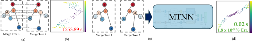
(a) Merge tree distances, where trees are matched and edited, are computationally heavy and slow to compute. This leads to analyses that can be a bottleneck in scientific workflows. (b) Here, we show an MDS visualization of a test dataset and the significant runtime necessary to produce a pair-wise distance matrix. (c) Rather than directly compute tree distances, we treat merge tree comparison as a learning task using our novel Merge Tree Neural Networks (MTNN) to calculate the similarity. (d) MDS of the same data as (b) using MTNN. This reduces comparison times by orders of magnitude (5, here) with extremely low error added compared to the state-of-the-art merge tree distance.

Introduction

A fundamental challenge in scientific visualization is analyzing and visualizing data, such as scalar fields, at speeds that support real-time exploration. Consider Topological Data Analysis (TDA) [17], which is now a critical component in many visualization pipelines due to its ability to extract and succinctly summarize structural information from complex datasets. TDA has been shown to effectively visualize [11, 23] and analyze a wide range of applications in chemistry [21, 9], neuroscience [30], social networks [2], material science [23], energy [39], and medical domains [27, 31, 49], to name a few. However, TDA approaches can be quite slow to compute due to their computational expense. Therefore, they are difficult to use in scenarios where a quick answer is needed for an analysis.

In particular, Merge Trees (MTs)[8, 17] serve as expressive topological descriptors that capture the complex structure of data, encoding the evolution of topological features with a history that records how their components merge. Despite being a powerful tool in various domains, the computational cost associated with distance calculations for merge trees has been a significant limitation. This is due to the core operation of computing the distance on merge trees needs to compare the optimal matching between each node of the merge trees. This matching is known to be NP-hard[1, 10]. Given the importance, yet great difficulty, of computing merge tree distances, a variety of metrics and pseudo-metrics have been proposed, such as functional distortion distance [8], edit distance [44], interleaving distance [20, 32], and distances based on branch decomposition and matching [40]. While many of these distance metrics are computationally challenging, it is worth noting that they are not universally NP-Hard [8]. Some metrics may have polynomial-time algorithms under specific conditions. However, these methods usually require complicated design and implementation based on discrete optimizations. Despite not being exponential, the time complexity is usually still polynomial or sub-exponential in the number of nodes in the merge trees.

In this work, we take a different approach. To address the challenge of fast comparisons, we re-frame it as a learning task. Once the similarities of merge trees become learnable, we can reduce the comparison runtime by avoiding the need to compute matchings between two MTs. To do so, we first need an encoder to map merge trees into a vector space, and learn this embedding model to position similar merge trees closely and dissimilar ones far apart in this space. We focus our investigation on Graph Neural Networks (GNNs) as our primary encoder, a technique extensively studied for graph embeddings yet unexplored for merge trees.

In the following, we introduce the first Merge Tree Neural Networks (MTNN) that uses GNNs to learn merge tree similarity. In particular, we design a neural network model that maps a pair of merge trees into a similarity score. At the training stage, the parameters involved in this model are learned by minimizing the difference between the predicted similarity scores and a ground truth, where each training data point is a pair of merge trees with their true similarity score. At the test stage, we can obtain a predicted similarity score by feeding the learned model with any pair of unseen merge trees.

To effectively learn both the structural and topological information of merge trees, we need to design the neural network architecture carefully. Traditional GNNs can only encode structural information of graphs, not merge trees. We introduce two key strategies to address this gap: firstly, we employ the Graph Isomorphism Network (GIN) as our encoder, which excels in identifying structural distinctions in merge trees due to its design for graph isomorphism tasks. Secondly, we develop an innovative topological attention mechanism designed to identify and highlight important nodes within a merge tree. This mechanism re-weight nodes based on their ground truth MT distance and nodes’ topological significance (persistence).

We conduct our experiments on five datasets: a synthetic point cloud, two datasets from time-varying flow simulations, one from a repeating pattern flow simulation, and one of 3D shapes. On all datasets, MTNN significantly enhances efficiency, accelerating the runtime by over 100 times while maintaining a low error rate when compared to a target MT similarity metric [51].

Our contributions can be summarized as follows:

• The first neural network model for merge tree similarity, called MTNN;

• A novel topological-based attention mechanism for GNNs;

• An evaluation that shows MTNN’s extremely precise($<0.1\%$ mean squared error) and fast ($>100\times$ speedup) similarity measures;

• An evaluation of the generalizability of trained models; and

• An open-source implementation for reproducibility .

The paper is organized as follows: Section 1 discusses related work, focusing on the computation of distance between merge trees and the application of learning methods for graph similarity. Section 2 provides the necessary preliminary background. In Section 3, we examine the using GNNs for merge trees. Our proposed model, MTNN, is detailed in Section 4. Section 5 presents our results, and Section 6 concludes the paper.

1 Related Work

Our approach is informed by two main areas of research: (1) the computation of distances between merge trees and (2) learning graph similarity using Graph Neural Networks (GNNs).

1.1 Merge Trees Distance

Many distances on merge trees exist: interleaving [32, 20], edit distance [16, 7], functional distortion [8], and the universal distance [6]. While these distances are valuable for their stability and discriminatory capabilities, computing these distances often becomes impractical due to their NP-Hard nature [1, 10].

Recent efforts aim to define more computationally feasible distances for merge trees. For instance, the edit distance on merge trees, as discussed in [44, 45], identifies the optimal edit operations between merge trees and has been experimentally shown to be more discriminative than both the bottleneck and one-Wasserstein [17] distances. The latter reference [45] introduced the local merge tree edit distance, specifically designed to analyze local similarities within merge trees. Despite the work in [47] demonstrating greater discriminative power than the previously proposed edit distances for merge trees, by employing a new set of improved edit operations, the computational cost is significantly higher, which hinders their practical application.

The interleaving distance requires an initial labeling of the merge trees, followed by the identification of the optimal matching between the labeled merge trees. This process, which establishes a computable metric known as the labeled interleaving distance, is introduced in [20]. Yan et al. [52] adapted this distance for practical use and incorporated geometric information into the labeling strategy in [51]. Similarly, Curry et al. [15] employed the Gromov–Wasserstein distance to label merge trees and compute the labeled interleaving distance.

Branch decomposition trees (BDTs) represent another method that first converts merge trees into BDTs (i.e., transferring edges of merge trees as nodes in a new tree), and then finds pairwise matching between these transformed trees [8, 40, 41, 48, 35, 34]. This process adds extra computational steps, further increasing complexity.

Applications utilizing merge trees distances, such as sketching [28] or encoding merge trees [35, 34], primarily operate in the original space, necessitating optimal matching between merge trees or their BDT variants. Machine learning has been used for merge trees in the work of Pont et al. [34], who applied neural networks to merge trees for compression and dimensionality reduction. Our work focuses on fast comparison. The previous work also uses a novel but classic auto-encoder with merge trees and BDTs as input, requiring a transformation step. In addition, their model is not designed to be generalizable across datasets, and their use of Wasserstein distance in training is computationally more intensive than our approach.

In summary, existing work either proposes a rigorous definition of distance with theoretical guarantees but with NP-Hard computation or describes a similarity measure with practical applications that still require optimal matching between merge trees. No existing work focuses on mapping merge trees into vector space for efficient comparison. The closest approach is the work of Qin et al. [38] who map topological persistence diagrams to a hash for fast comparison. Merge trees are a more expressive and more complex topological abstraction than these diagrams.  In our work, we utilize GNNs to map the merge trees into a vector space and re-frame merge tree comparison as a learning task.

1.2 Learning Graph Similarity

Graph similarity computation is a fundamental problem in graph theory. The graph edit distance (GED) [19] is a widely recognized metric for graph similarity, defining the minimum number of edit operations required to transform one graph into another. Despite its popularity, GED is known to be an NP-Hard problem [53].

With the advancements in Graph Neural Networks (GNNs), it is now possible to encode graphs into vector spaces effectively [26, 24, 50]. This capability allows GNNs to transform the GED into a similarity score quickly, employing an end-to-end framework to learn the graph representation that maps the given two graphs to their similarity score. In this context, a graph similarity problem involves mapping two graphs with a known similarity metric (e.g., GED) to their respective similarity score.

A common approach in this area is the use of a Siamese neural network architecture [14], which processes each graph independently, but in parallel, to aggregate information. A feature fusion mechanism then captures the inter-graph similarities, and a Multi-layer Perceptron (MLP) is applied for regression analysis. This method is typically trained in a supervised manner using the Mean Square Error (MSE) loss against a ground truth similarity scores.

Many GNN-based approaches for learning graph similarity have great promise due to the competitive performance in both efficiency and efficacy [29, 4, 5, 37]. For example, the Graph Matching Network (GMN) [29] is the first deep graph similarity model, which computes the similarity between two given graphs by a cross-graph attention mechanism. SimGNN [4] turned the graph similarity task into a regression task, and leveraged the GCN layers with self-attention-based mechanism on the model.

However, despite the growing popularity of GNN-based methods for graph similarity, their application to topological descriptors like merge trees has not been explored. Our research establishes the initial connection between GNNs and merge trees, potentially laying the groundwork for future developments in machine learning and TDA.

2 Preliminaries

In this section, we outline the foundational concepts of this work, beginning with merge trees induced by scalar fields and the common distances used for topological comparisons. Then, we describe Graph Neural Networks (GNNs), which serves as the core architecture for encoding merge trees for topological comparison.

2.1 Scalar Fields and Merge Trees

Consider a dataset represented as $(\mathbb{X},f)$, where $\mathbb{X}$ denotes a topological space, and $f:\mathbb{X}\rightarrow\mathbb{R}$ denotes a scalar function, which is a continuous real-valued function. This function $f$ assigns a real number to each point in $\mathbb{X}$, reflecting a characteristic of interest within the dataset. This is often referred to as a scalar field.

An equivalence relation $\sim_{f}$ is defined on $\mathbb{X}$, where $x\sim_{f}y$ if both $x$ and $y$ belong to the same connected component of the sub-level set $\mathbb{X}_{a}$ for a threshold value $a$ in $f$. Consequently, two points are equivalent under $\sim_{f}$ if they exhibit a shared characteristic under the threshold $a$.

This leads to the definition of $\mathcal{T}_{f}^{-}:=(\mathbb{X}_{a},f)$ as the join tree for the dataset $(\mathbb{X},f)$. The join tree encapsulates how dataset components merge as the threshold $a$ varies. The split tree $\mathcal{T}_{f}^{+}:=(\mathbb{X}_{a},f)$ is similarly constructed using super-level set to depict component splits with changing thresholds. Each of these two trees is called a merge tree $\mathcal{T}_{f}:=(\mathbb{X}_{a},f)$, illustrating the evolution of topological features in relation to $f$. In this work, we use join trees to capture the connectivity of sub-level sets, with the global maximum being the tree’s root. Example join tree for a 1D functions are shown in Fig. 1.

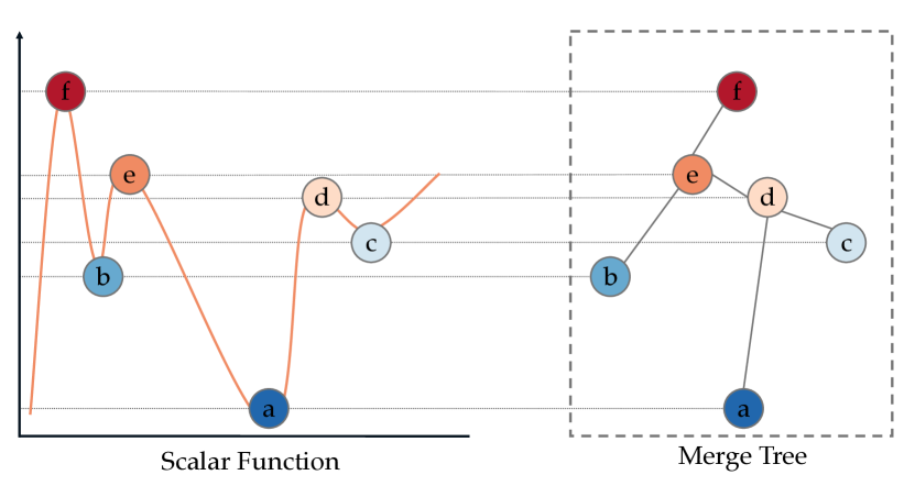
Figure 1: An illustration of merge trees. From left to right, critical points in the scalar function are connected by an orange line, showcasing how these points merge and connect topologically. Right, presenting the corresponding merge trees of sub-level set filtration.

Persistence

Persistence is a quantity derived from persistent homology [17] that tracks the lifetime of a topological feature. This is often important in analysis. For instance, low persistence features are often deemed to be noise, while high persistence features are considered to encode important topological properties. In the context of our work, persistence will be used to track the evolution of connected components of a sub-level set of a scalar function. A persistence pair ($b,d$) represents a topological feature that is born in the sub-level set $\mathbb{X}_{b}$ and dies in the sub-level set $\mathbb{X}_{d}$. $b$ and $d$ correspond to the critical points $m$ and $s$ where $b=f(m)$ and $d=f(s)$. In our join trees, a feature will be born at a minimum and dies when it merges with an older, in terms of $f$, feature. The persistence of such a pair is defined as the difference in function value at the two critical points, $d-b$.

2.2 Distance on Merge Trees and Graphs

Below, we first define graph edit distance, which GCNs primarily focus on reproducing. We then describe how edit distance on merge trees differs. Finally, we describe the distance we use as our ground truth, interleaving distance.

Graph Edit Distance

The Graph Edit Distance (GED) [19] between two graphs $G_{1}=(V_{1},E_{1})$ and $G_{2}=(V_{2},E_{2})$ is the minimum cost of transforming $G_{1}$ into $G_{2}$ using node and edge insertions, deletions, and substitutions. It’s defined as:

$$D_{e}(G_{1},G_{2}):=\min_{S\in O}\left\{\sum_{op\in S}c(op)\right\},$$

where $O$ represents the set of all valid sequences of graph edit operations that transform $G_{1}$ into $G_{2}$, $S$ is a specific sequence of graph edit operations from $O$, and $c(op)$ is the cost function that assigns a non-negative real number to each edit operation $op$ in the sequence $S$. This operation could be the insertion, deletion, or substitution of a node or an edge.

Each operation $op$ has an associated cost, and $\sum_{op\in S}$, the total cost of a sequence $S$, is the sum of the costs of its individual operations. The GED is then determined by finding the sequence $S$ with the minimum total cost that transforms $G_{1}$ into $G_{2}$.

Edit Distance on Merge Trees

The edit distance between merge trees builds on tree edit distance, which is a specific case of GED where the cost operation is only on nodes. Given two merge trees, denoted as $\mathcal{T}_{1}$ and $\mathcal{T}_{2}$, it is defined as [44]:

$$D_{e}(\mathcal{T}_{1},\mathcal{T}_{2}):=\min_{S\in O}\{\delta(S)\},$$

where $O$ represents the set of valid tree edit operations, and $S$ represents a sequence of these tree edit operations that transform $\mathcal{T}_{1}$ into $\mathcal{T}_{2}$. The cost function $\delta$ assigns a non-negative real number to each edit operation, which is defined as [44]:

$$\begin{array}[]{lll}\delta(m\rightarrow s)=\min\left\{\begin{array}[]{cc}\max(|b_{m}-b_{s}|,|d_{m}-d_{s}|),\\ \frac{(|d_{m}-b_{m}|+|d_{s}-b_{s}|)}{2}\end{array}\right\}\\ \delta(m\rightarrow\lambda)=\frac{|d_{m}-b_{m}|}{2}\\ \delta(\lambda\rightarrow s)=\frac{|d_{s}-b_{s}|}{2}\end{array}$$

where $\lambda$ denotes the empty set. $m$ and $s$ are node $m\in\mathcal{T}_{1}$ and $s\in\mathcal{T}_{2}$, The first cost is for a node relabel operation from $m$ to $s$. Next is deleting a node $m$. The last cost is adding a node $s$.

This is similar to GED, but the cost is formulated to account for topological persistence. Consider nodes $m\in\mathcal{T}_{1}$ and $s\in\mathcal{T}_{2}$, each node encodes a topological feature, $(b_{m},d_{m})$ and $(b_{s},d_{s})$. In particular, $b_{m}$ is the function value where $m$ is born. $d_{m}$ is the function value where $m$ dies. For sublevel sets, $b_{m}<d_{m}$. This distance computation is shown in Fig. 2.

Interleaving Distance on Merge Trees

To compute the interleaving distance on merge trees, the trees need to be labeled first. A labeled merge tree, denoted as $T=(\mathcal{T},\pi)$, including a merge tree $\mathcal{T}$ with a labeling $\pi:[a]\rightarrow V_{\mathcal{T}}$ where $[a]$ is the set of labels, $\{1,...,a\}$, and $V_{\mathcal{T}}$ is the set of merge tree vertices [20]. $\pi$ only needs to be surjective since a vertex can have multiple labels. The interleaving distance on labeled merge trees is calculated based on the induced matrix $T_{M}(\mathcal{T},\pi)$. This matrix also can be referred to as the least common ancestor (LCA) matrix and defined as:

$$T_{M}(i,j)=f(LCA(\pi(i),\pi(j)),$$

where $f(LCA(\cdot))$ denotes the function value of LCA of a pair of vertices with labels $i$ and $j$, $1\leq i,j\leq a$. Given two labeled merge trees $T_{1}=(\mathcal{T}_{1},\pi_{1})$ and $T_{2}=(\mathcal{T}_{2},\pi_{2})$ that share the same set of labels, $[a]$, the interleaving distance between labeled merge trees is defined as:

$$D_{i}(T_{1},T_{2})=\|T_{M}^{1}-T_{M}^{2}\|_{\infty},$$

where $\|T_{M}\|=\max_{ij}|T_{Mij}|$ is the $L_{\infty}$ norm. In [51], they proposed geometry-aware labeling strategies and for brevity, we refer the reader to their paper for those details. But, at a high level, their labeling minimizes a cost function that accounts for the geometric structure of the tree along with the function value differences between nodes in the tree. In this way, topological persistence is encoded into the labeling strategy. Interleaving distance is used as the ground-truth merge tree distance in our training.

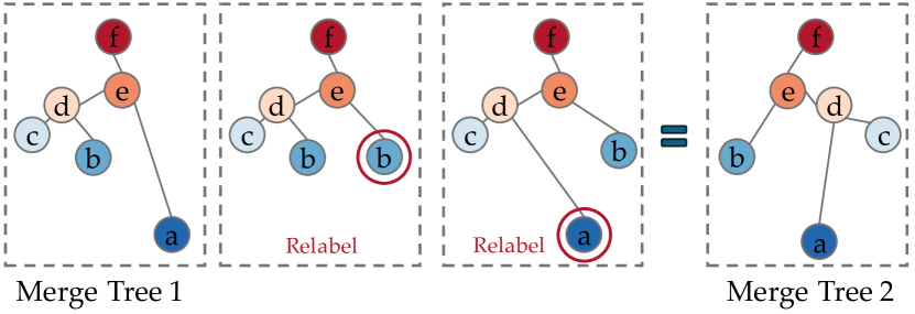
Figure 2: Edit distance on merge trees example. The transformation from merge tree 1 to merge tree 2 needs two node relabel operations, where the relabeled node is highlighted in the red circle.

2.3 Graph Neural Networks (GNNs)

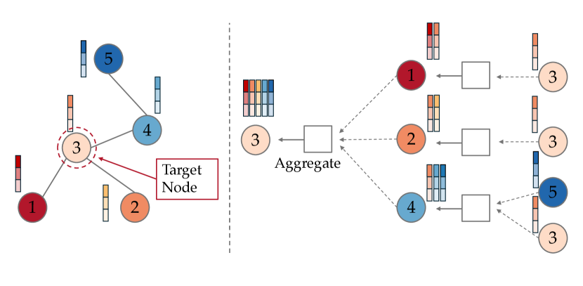
Figure 3: Example of the GNNs process for a single node. Left: a graph with node features. Right: message function and update function for the target node 3. This node receives information from its directly connected neighbors — nodes 1, 2, and 4. Notably, node 4 further communicates a message from its adjacent node 5. In the end, the feature of node 3 is updated by aggregating all incoming messages.

Given a graph $G=(V,E)$ with nodes $V$ and edges $E$, where each node $v\in V$ has an initial feature vector $h_{v}^{(0)}$, GNNs update the feature representation of each node by leveraging the structural context provided by the graph [24]. In particular, each node aggregates features from its neighbors (Message Function), updates its own features (Update Function), and finally produces an embedding (Embedding) that represents either the node’s or the entire graph’s comprehensive features. As Fig. 3 shows, the message function is responsible for aggregating information from a node’s neighbors, which is then integrated into the node’s feature vectors through the update function.

Message Function: The message function aggregates features from neighboring nodes. For a node $v$, the message function $M$ can be defined as:

$$m^{(l+1)}_{v}=\sum_{u\in\mathcal{N}(v)}M(h^{(l)}_{v},h^{(l)}_{u},e_{vu}),$$

where $h^{(l)}_{v}$ is the feature vector of node $v$ at layer $l$, $\mathcal{N}(v)$ denotes the neighbors of $v$, and $e_{vu}$ represents the edge features between nodes $v$ and $u$.

Update Function: The update function $U$ integrates the aggregated messages with the node’s current state to compute its new state:

$$h^{(l+1)}_{v}=U(h^{(l)}_{v},m^{(l+1)}_{v}),$$

where $h^{(l+1)}_{v}$ is the updated feature vector of node $v$ at layer $l+1$.

Embedding: After processing through $L$ layers of the GNN, the final embedding $z_{v}$ for a node $v$ is obtained, which can be used for downstream tasks like classification or clustering:

$$z_{v}=h^{(L)}_{v}.$$

For a whole graph embedding, an aggregation function (e.g., sum, mean, or max) is applied over all node embeddings to produce a single vector representing the entire graph. Through these mechanisms, GNNs offer a powerful framework for learning from graph-structured data, which we adapt to the context of merge trees for our topological comparison.

3 GNNs Meet Merge Trees

This section describes our methodology for adapting GNNs to merge trees. While GNNs have demonstrated effectiveness in learning on graph-structured data, the application to merge trees is not directly translatable due to unique topological characteristics inherent to merge trees. See Fig. 4. To address this, we enrich the node features with topological information. Specifically, we assign an attribute to each node derived from its scalar function value. Moreover, our objective goes beyond learning the structure of merge trees; we are focused on a more complicated task, learning merge tree distance. To this end, we employ GCN similarity [4], a model initially designed for graph similarity learning, adapting it to the context of merge trees. This adaptation allows us to establish a baseline for our approach. More details are given below.

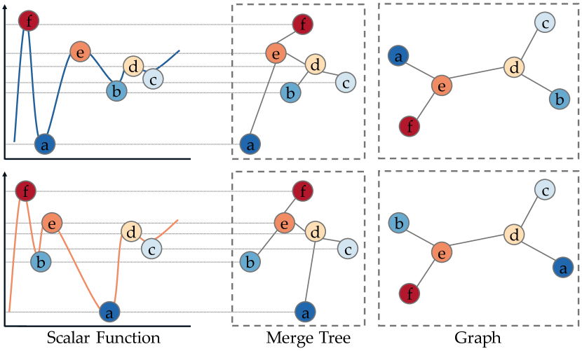
Figure 4: An illustration of two merge trees and their graph structure. From left to right: critical points (dots) in two scalar functions, showcasing how these points merge and connect topologically. In the middle are corresponding merge trees, highlighting structural differences. Finally, the graph structure of the two merge trees is identical but differs in function value labels.

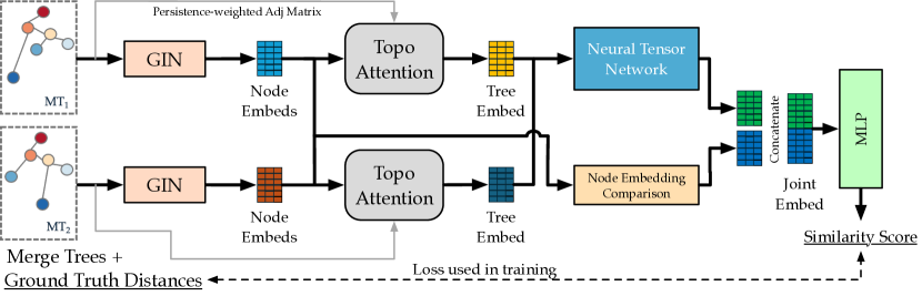
Figure 5: The architecture of our Merge Tree Neural Networks (MTNN) operating on a pair of merge trees ($MT_{1,2}$). First, adjacency matrices for each merge tree with node feature are weighted by function value and are fed into a GIN. This produces node embeddings for both. Next, our topological attention produces tree embeddings from the node embeddings. A persistence-weighted adjacency matrix is an additional input for this step. The node embeddings are then compared, and tree embeddings are fed into a neural tensor network. These outputs are concatenated to form a joint embedding. This joint embedding is fed into a multi-layered perceptron (MLP) to produce a similarity score. This score is compared to the ground truth distance (normalized) in the training loss function.

3.1 Graph Convolutional Network (GCN) Similarity

Following [4], the computation of the merge tree similarity has the following steps: (1) a GNN transforms the node of each tree into a vector, this is called node embedding; (2) a tree embedding is computed using attention-based aggregation; (3) a joint embedding is obtained by comparing node and tree-level embeddings to capture a comprehensive similarity between the merge trees. (4) Finally, the joint embedding is fed into a fully connected neural network to get the final similarity score. Below, we provide more details on these steps.

Initialization

The inputs to our approach are merge trees, stored as adjacency matrices. A nodes of a merge tree are weighted with the normalized ($[0,1]$) function value. The ground truth distance is also normalized.

Node Embedding Computation

For the first step, we compute a node embedding using a Graph Convolutional Network (GCN)[26], a type of GNN that updates the node features by aggregating features from their neighbors. The formula for node level updates in a GCN can be expressed as:

$$h_{v}^{(l+1)}=\sigma\left(\sum_{u\in\mathcal{N}(v)\cup\{v\}}\frac{1}{\sqrt{\hat{d_{v}}\hat{d_{u}}}}h_{u}^{(l)}W^{(l)}+b^{(l)}\right)$$

where $h_{v}^{(l+1)}$ is the feature vector of node $v$ at layer $l+1$; $\sigma$ is a non-linear activation function, such as ReLU$(x)=max(0,x)$; $\hat{d_{v}}$ is the degree of node $v$, plus 1 for self-loops; $W^{(l)}$ is the weight matrix at layer $l$; and $b^{(l)}$ is the bias at layer $l$. Given a pair of merge trees $\mathcal{T}_{i},\mathcal{T}_{j}$, We obtain the node embedding $h_{iv}$ and $h_{jv}$ for each node of $\mathcal{T}_{i}$ and $\mathcal{T}_{j}$ via the GCN.

Tree Embedding

For tree embeddings, we use attention-based aggregation. Attention-based aggregation is designed to assign weights to each node based on a given similarity metric. $h_{n}\in\mathbb{R}^{m}$ is the embedding of $n$-th node, where $m$ is the size of embedding. The global context $c\in\mathbb{R}^{m}$ is obtained as

$$c=\tanh(\frac{1}{|V|}\sum_{n=1}^{|V|}h_{n}W_{c}),$$

where $|V|$ is the number of nodes and $W_{c}\in\mathbb{R}^{m\times m}$ is a learnable weight matrix. Next, each node should receive attention relative to this global context. The attention-weight embedding for a node is calculated as

$$h^{*}_{n}=\sum_{n=1}^{|V|}\mu(h_{n}^{T}c)h_{n}$$

where $\mu(\cdot)$ is the sigmoid function. The tree-level embedding $H^{*}$ is aggregated from all re-weighted node embeddings, $h^{*}$.

Joint Embedding Computation

For step three, the joint embedding is obtained by comparing both tree-level and node-level embeddings. We first describe how to compare the tree-level embedding using Neural Tensor Networks (NTN) following [42]:

$$D_{tree}(H_{i}^{*},H_{j}^{*})=\sigma(H_{i}^{*T}W_{t}^{[1:K]}H_{j}^{*}+V_{w}[H_{i}^{*}\cdot H_{j}^{*}]+b_{t})$$

where $D_{tree}$ is the tree-level vector that encodes similarity, $\sigma(\cdot)$ is an activation function, $W_{t}^{[1:K]}\in\mathbb{R}^{m\times m\times K}$ is a weight tensor, $[H_{i}^{*}\cdot H_{j}^{*}]$ is concatenation operation between $H_{i}^{*},H_{j}^{*}$, $V_{w}\in\mathbb{R}^{K\times 2m}$ is a weight vector, and $b_{t}\in\mathbb{R}^{K}$ is a bias vector. Here $K$ is a hyperparameter for the size of $D_{tree}$. In summary, the NTN provides a measure of similarity between two tree embeddings.

To assess node-level similarities, we compare the node embeddings from two trees, $\mathcal{T}_{i}$ and $\mathcal{T}_{j}$. Letting $N_{i}$ and $N_{j}$ be the number of nodes in $\mathcal{T}_{i}$ and $\mathcal{T}_{j}$, respectively, this comparison yields an $N_{i}\times N_{j}$ similarity matrix. Specifically, the similarity matrix $D_{node}$ is calculated as $D_{node}=\sigma(H_{i}H_{j}^{T})$, where $H_{i}\in\mathbb{R}^{N_{i}\times m}$ and $H_{j}\in\mathbb{R}^{N_{j}\times m}$ are each the matrix of node embeddings for trees $\mathcal{T}_{i}$ and $\mathcal{T}_{j}$. $\sigma(\cdot)$ is an activation function that normalizes the scores into the same range, $(0,1)$. To address the discrepancy in node counts between trees, we zero-pad the trees with fewer nodes. This step ensures that the size difference between trees is factored into the similarity assessment.

While the size between trees is the same for each pair, the size between pairs does differs. Following the methodology in [4], we convert this matrix into a histogram $\text{hist}(D_{node})\in\mathbb{R}^{B}$, where $B$ is a predefined number of bins. This histogram representation standardizes the similarity matrix’s size, facilitating comparison across tree pairs.

Final

In the final step, we combine the tree-level similarity $D_{tree}(H_{i}^{*},H_{j}^{*})$ with the histogram $\text{hist}(D_{node})$ as the joint embedding. A fully connected neural network then processes this embedding to produce the ultimate similarity score between the merge trees pair in the $[0,1]$ range. This approach serves as the baseline model in our study, with its performance detailed in Section 5.

3.2 Graph Isomorphism Network (GIN) Similarity

While our results with GCN similarity on merge tree comparison are encouraging, the variation in the number of nodes between two merge trees plays a significant role in distinguishing them. To emphasize the differences in node count, we further improved the model by replacing the standard GCN with a Graph Isomorphism Network (GIN) for the node embedding computation. As presented in [50], GIN is adept at capturing distinct graph structures. For instance, it can reproduce the Weisfeiler-Lehman test for graph isomorphism.

The update rule for a GIN is:

$$h^{(l+1)}_{v}=\text{MLP}^{(l)}\left((1+\epsilon^{(l)})\cdot h^{(l)}_{v}+\sum_{u\in\mathcal{N}(v)}h^{(l)}_{u}\right)$$

where $h^{(l+1)}_{v}$ is node $v$’s feature vector at layer $l+1$, $\text{MLP}^{(l)}$ denotes a multi-layer perceptron, and $\epsilon^{(l)}$ is a tunable parameter that balances the node’s own features with its neighbors’. The summation aggregates the features of node $v$’s neighbors, enhancing the representation with local structural information.

By deploying a GIN, we enriched the model with a more complicated understanding of node differences across merge trees. In our work, we incorporated three GIN layers to optimize node feature learning and report the performance in Section 5. The result shows that this approach improves performance significantly over the GCN model.

However, it’s crucial to note that GIN’s capacity for graph isomorphism may not fully capture the subtleties of MT comparisons. For instance, two merge trees might be structurally the same yet distinct in a topological sense. We extend GIN into a more customized network for merge trees to address this. This is our final approach, called a Merge Tree Neural Network (MTNN).

4 Merge Tree Neural Networks (MTNN) Similarity

As mentioned earlier, effectively capturing the topological characteristics of merge trees is crucial for learning their similarities using GNNs. We have previously incorporated the function value for the nodes in a merge tree. However, we haven’t yet addressed the inclusion of another important topological measure: the persistence of features in merge trees. To integrate this persistence information, we use a persistence-weighted adjacency matrix for tree embedding, which we detail in Section 4.1. Following that, in Section 4.2, we describe how to apply this weighted matrix in our model effectively, and we outline the learning process in Section 4.3. An overview of the model is provided in Fig. 5.

4.1 From Persistence to Edge Features

In the context of a merge tree, $\mathcal{T}$, each edge connecting nodes $s$ and $m$ represents a persistence pair, denoted as $(f(s),f(m))$, which we utilize as an edge feature in our model. This approach, while useful, captures only incomplete topological information, as certain topological features span across multiple edges forming a path in the merge tree. To summarize the full topological characteristics of a merge tree, we introduce a persistence-weighted edge adjacency matrix $\hat{E}$. This matrix is formulated by considering the function value differences between connected nodes, encompassing connections to neighbors. This enhancement allows us to extend our analysis from direct pairs like $(f(s),f(m))$ to broader connections, capturing $(f(s),f(\mathcal{D}(m))\cup f(m))$, which includes node $m$ and its descendants, $\mathcal{D}(m)$. Fig. 6 illustrates how we accomplish this construction.

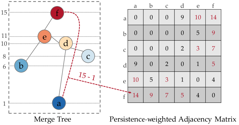
Figure 6: An example of our persistence-weighted adjacency matrix. All edges are weighted by persistence. Values in red denote values for nodes not directly connected in the merge tree.

To integrate this persistence-weighted matrix, we tested two methods: (1) Incorporating it into GNN architectures like GIN or GCN; (2) Utilizing it in an attention-based aggregation to map node embeddings to tree embeddings.

Option (1) introduces modified edges (referred to as "pseudo" edges) to include persistence information. Consequently, this approach updates node features by utilizing neighbor features via the adjacency matrix. However, this modification changes the original merge tree structure in the message updates function of GNNs due to the introduction of pseudo edges.

To preserve the original merge tree structure while incorporating persistence information, we choose method (2). This approach leverages the persistence-weighted matrix in an attention-based aggregation process, mapping node embeddings to tree embeddings. Here, node re-weighting is informed by their persistence, but not exclusively so. We train the weight matrix to consider both the persistence information and the overall merge tree distance, ensuring a balanced integration of topological features.

4.2 Topological Attention

This section outlines the design of topological attention, leveraging the persistence-weighted adjacency matrix $\hat{E}$.

Building on the attention-based aggregation discussed in Section 3.1’s Tree Embedding, we reformulate the global context vector $c$. We integrate the topological information as:

$$Norm=\sum_{k=1}^{|V|}\sum_{l\in\mathcal{N}(k)}\hat{e}_{kl},$$

$$c=\tanh\left(\frac{1}{|V|}\sum_{n=1}^{|V|}\left(\frac{\sum_{u\in\mathcal{N}(n)}\hat{e}_{un}}{Norm}\right)h_{n}W_{c}\right)$$

where $u\in\mathcal{N}(n)$ is the neighbor node of $n$, $\hat{e}_{un}\in\hat{E}$ is the persistence-weighted edge feature of $u$ and $n$, $h_{n}$ is the embedding of $n$-th node, $|V|$ is the number of nodes, and $W_{c}$ is a learnable weight matrix . To further break down the the formula above, we have the local weighting factor for each node $v$, the sum $\sum_{u\in\mathcal{N}(v)}\hat{e}_{uv}$ computes the total edge weight connected to $v$. By dividing this sum by the normalization term $Norm$, we normalize the local weighting with respect to the total edge weights in the tree, ensuring the scale of the features remains consistent. Then, we use the same calculation as the previous attention-based aggregation.

4.3 MTNN Learning

Training of the MTNN uses a Siamese network architecture, utilizing GINs as encoders to transform input merge trees into node embeddings. We generate joint embeddings by combining node and tree embeddings, where the tree embedding is derived using a topological attention-based aggregation. This aggregation reweights nodes according to their topological features. Subsequently, we employ an MLP-based regression network to map the joint embedding to the ground-truth similarity score between the merge trees. The model is trained to minimize the Mean Squared Error (MSE) loss, defined as:

$$L=\frac{1}{D}\sum_{i,j\in D}(\text{MLP}(H_{ij}^{*})-s_{ij})^{2}$$

Here, MLP denotes the MLP-based regression network, and $D$ is the set of all training merge trees pairs, $H_{ij}^{*}$ is the joint embedding and $s_{ij}$ is the ground-truth MT distance.

Table 1: Number of merge trees (MTs), $\tau$ used, and their range in node counts after simplification.

Dataset	# of MTs	$\tau$	# of Nodes
MT2k	2000	0.1	[8,191]
Corner Flow	1500	0.2	[24,30]
Heated Flow	2000	0.06	[12,27]
Vortex Street	1000	0.05	[56,62]
TOSCA	400	0.01	[12,78]

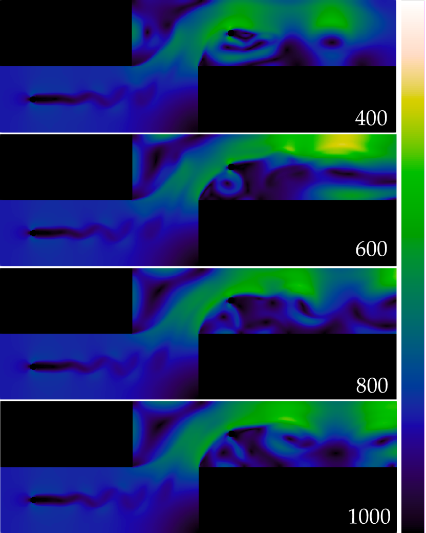
Figure 7: Time steps of the 2D viscous Corner Flow simulation dataset.

5 Results

While our proposed approach can be generalized to different merge tree distances, we have chosen the state-of-the-art distance metric from [51] as our ground truth. This metric is noted for its efficient computation and is accompanied by an accessible open-source implementation. As mentioned, this distance is normalized to fall within the $[0,1]$ range to coincide with a similarity score. To compare the quality of our MTNN similarity in reproducing [51], we use Mean Squared Error (MSE) as our evaluation metric.

5.1 Datasets

We evaluate MTNN on five datasets: MT2k, Corner Flow, Heated Flow, Vortex Street, and TOSCA. All datasets, except MT2k, were chosen because they have previously been used in merge tree distance research [51, 44]. Interestingly enough, three [51] are from a similar domain: 2D flow simulations. This allows us to test the general applicability of a trained MTNN model across the same domain. Following the previous work, each we de-noise each merge tree for a pre-determined threshold $\tau$ as follows: given a node pair $(s,m)$, where $s$ is a local minimum and $m$ is its emerging saddle point, the persistence is computed for each pair, $p=f(m)-f(s)$, where $f(s)$ and $f(m)$ are the function values at node $s$ and $m$, respectively. If $p$ is less than $\tau$, then node $s$ and its connecting edge are removed with the children of $s$ being directly connected to $m$. Nodes are processed in reverse order of persistence. This results in the merge tree having fewer nodes and edges, with only the significant features remaining. More information on merge tree simplification can be found in [17, 51, 44]. The number of merge trees and range of node counts after simplification for each are summarized in Table 1.

As mentioned, all merge trees used are join trees., although the approach could have also easily used split trees. Finally, we used the standard random split, $80\%$ and $20\%$, of all the merge trees as training and testing sets for each dataset.

MT2k

This dataset is 2000 synthetic 3D point clouds with two distinct classes. The first features three noisy tori, and the second class contains three noisy tori plus one noisy sphere. Each point cloud is constructed by synthetically sampling 100 points from the respective geometric shapes. Random noise is added during the sampling to ensure the uniqueness of each data point. Corresponding merge trees are constructed for each point cloud to represent their topological features. We apply a persistence threshold ($\tau=0.1$) in the merge tree simplification process.

Corner Flow

This dataset is 1500 time steps from a simulation of 2D viscous flow around two cylinders [36, 3]. Following [51], we generate a set of merge trees from the vertical component of the velocity vector fields. We also use the same persistence threshold ($\tau=0.2$) for merge tree simplification as the previous work.

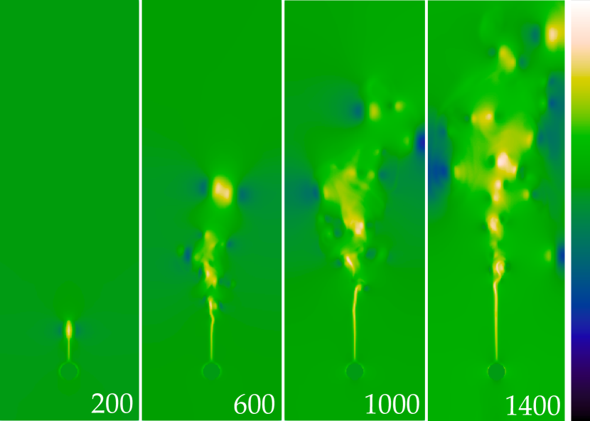
Figure 8: Time steps of the 2D Heated Flow simulation dataset.

Heated Flow

This dataset is from a simulation of the 2D flow created by a heated cylinder using a Boussinesq Approximation [36, 22]. Following [51], we convert each time instance of the flow into a scalar field using the magnitude of the velocity vector. The persistence simplification threshold used here is ($\tau=0.06$), the same as the previous work.

Vortex Street

This is an ensemble of 2D regular grids [36, 22], each with a scalar function defined on the vertices to represent flow turbulence behind a wing, creating a 2D von-Kármán vortex street. Following [51], we use the velocity magnitude field to generate merge trees and apply a persistence simplification with the threshold ($\tau=0.05$) to the merge trees. See Fig. 10.

TOSCA

This dataset [12] contains a collection of different, non-rigid shapes of animals and humans. Following [44], we compute the average geodesic distance field on the surface mesh. Like the previous work, persistence simplification is used with the threshold ($\tau=0.01$).

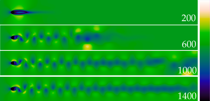
Figure 9: Time steps of the 2D von-Kármán Vortex Street dataset.

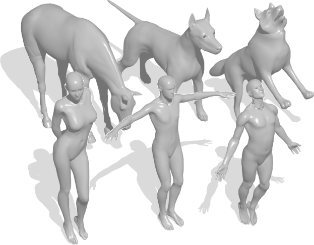
Figure 10: Example 3D models from the TOSCA dataset.

5.2 Implementation Details

Merge trees are computed using TTK [46] and Paraview [43] is used for dataset visualization. Our implementation utilizes PyTorch [33]. We employ a 3-layer GIN [50] as the encoder network with ReLU activation function with all weights initialized randomly. The output dimensions for the 1st, 2nd, and 3rd GIN layers are 64, 32, and 16, respectively. In the NTN layer, we specify $K=16$. Following the approach in [4], we use 16 histogram bins for pairwise node embedding comparisons. For training, we choose the Adam optimizer [25], setting the learning rate to $0.001$ and the weight decay to $0.0005$. The model is trained with a batch size of $128$ over 100 epochs. All datasets are converted into standard dataloaders compatible with PyTorch Geometric (PyG) [18] for GNN processing. To present each technique in the best light, we computed all timings for our ground truth distance [51] on a machine with a 16-Core (8P/8E) Intel I9-12900K CPU @ 5/4 GHz with 32 GB memory, as the approach benefits most from multiple cores. MTNN timings are computed on a machine equipped with a 6-core Intel i7-6800K CPU @ 3.50GHz, 68GB of memory, and an Nvidia 3090Ti GPU, since it benefits most from a better GPU.

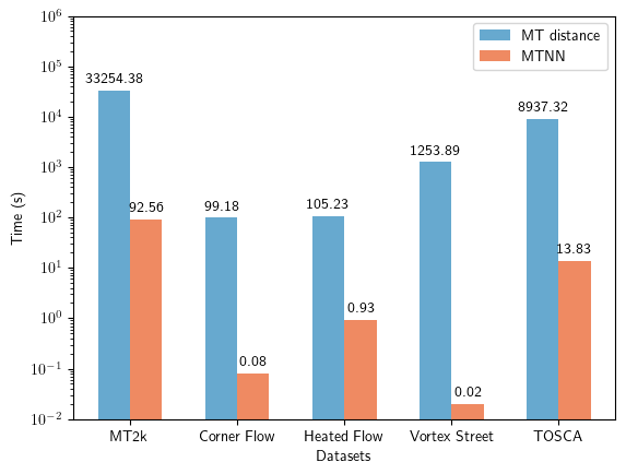
Figure 11: Comparison of computational times for merge tree distance [51] and MTNN across different datasets. Times are presented in log scale. (Runtime for merge tree distance is computed with 16 cores)

5.3 Evaluation Results

We evaluate the proposed approach from two perspectives: effectiveness and efficiency. For effectiveness, we compute the distance between the predicted similarity and our ground truth distance [51] using Mean Squared Error (MSE), the standard for learned graph similarity validation. For efficiency, we record the wall time needed to compute the full pairwise similarity matrix for the testing set.

Effectiveness

Table 2 provides quality results for our machine learning approaches. This includes the initial GCN, improved GIN, and our final MTNN model with topological attention. This study focused on models trained and tested on the same (split) dataset. For readability, we have scaled each by $10^{3}$. Since both our ground truth and similarity output are in the $[0,1]$ range, the error is $<0.1\%$. Therefore the MSE between our approach and the ground truth is extremely low. The table also shows that the GIN model consistently outperforms our initial GCN model. Finally, our MTNN model in this scenario is comparable to or better than our GIN formulation. Our MTNN approach outperforms GIN in cases of higher GIN error, but has diminishing returns as the error lowers.

Table 2: MSE error for test datasets for GCN, GIN, and our MTNN networks. Each dataset was trained on a standard split of the source data. All results are scaled by $10^{3}$ for readability, as our errors are extremely low. This means that all trained networks reproduce the similarity very close to the ground truth. Our MTNN network improves on the quality of the reproduction, but not in cases where GIN error is already extremely low.

Dataset	GCN	GIN	MTNN
MT2k	0.53819	0.18996	0.10408
Corner Flow	65.23393	0.00145	0.00312
Heated Flow	36.36125	0.00468	0.00263
Vortex Street	470.82582	0.00008	0.00018
TOSCA	12.60986	0.01542	0.00986

Table 3 explores the generalizability of our models. As before, all error results are scaled by $10^{3}$ for readability. First, we tested the quality of our similarity measure in a scenario where the model is trained on merge trees from one data type but is applied to other types. For this, we used a model trained on the synthetic MT2k dataset. The table shows that the error is quite low even though we use merge trees from a 3D point cloud on very different data (i.e., 2D flows and 3D shapes). MT2k is also a fairly limited and constrained data source. The quality of these results shows that the MTNN model has the potential to be generally applied.

Table 3: MSE error for our datasets on models trained on other data. On the left is the error of applying the MT2k-trained model. On the right is a new model trained with a mix of Corner Flow, Heated Flow, and Vortex Street. Our topological attention are most effective in this scenario, leading to the lowest error values for each model (bold). Our synthetic MT2k performs best on the 3D shape dataset, while the model trained on the 3 separate flow datasets is best for the flow data (underlined). All results are scaled by $10^{3}$ for readability, so all models return a low error with most $<0.1\%$.

	Trained on MT2k			Trained on CF + HF + VS
	GCN	GIN	MTNN	GCN	GIN	MTNN
Corner Flow	83.93713	0.03507	0.01795	17.20086	1.60534	0.00862
Heated Flow	57.93813	0.16013	0.00501	32.83913	0.23754	0.00573
Vortex Street	541.03814	113.24254	3.78652	178.93201	63.92713	0.17532
TOSCA	27.9381	3.17674	0.2016	37.8729	8.03914	1.63408

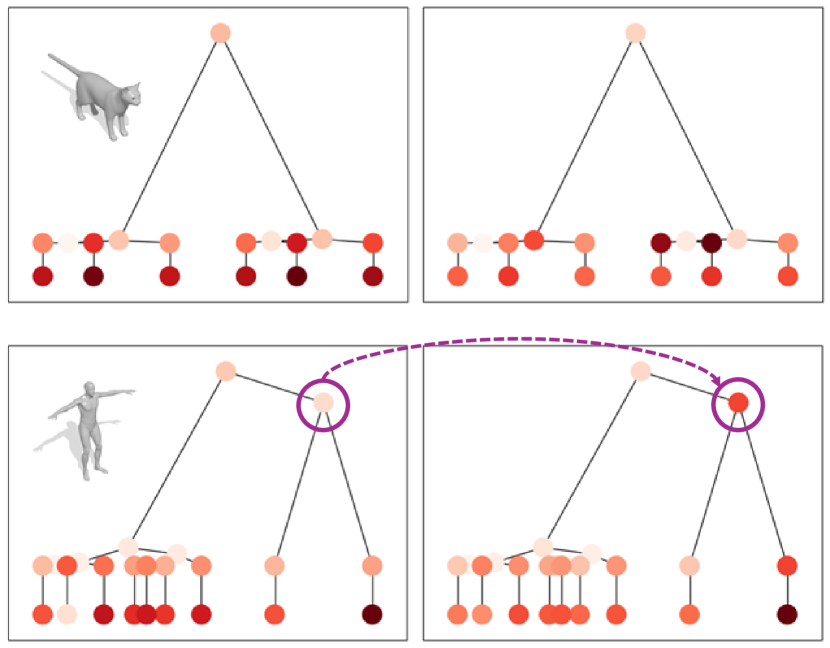
Figure 12: Topological attention on two merge trees from the TOSCA dataset. Left: node importance without topological attention, using the GIN model. The node colors indicate their relative importance when comparing the two examples. Right: node importance with topological attention using the MTNN model. The GIN model already emphasizes structural differences between the two merge trees. But, the introduction of topological attention further emphasizes these differences, re-weighing the nodes in the high persistence feature highlighted in purple.

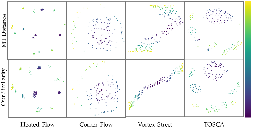
Figure 13: Results from multidimensional scaling (MDS) analysis. Two MDS maps represent each dataset. On the top are the maps created using a similarity matrix based on the ground truth merge tree (MT) distance [51]. On the bottom are maps generated from a similarity matrix of MTNN. The coloring indicates the mean distance, showing how close or far points are from each other in the MDS space. Comparing the two maps shows similar patterns in colors and point arrangements. This similarity indicates that MTNN effectively learns and reflects the relationships between points.

Next we tested how a model trained on a mix of like data performs. In this scenario, we trained on the combination of the Corner Flow, Heated Flow, and Vortex Street training sets, each sampled equally by 800. This model was then applied to our test sets. As is shown, the error is very low for our vector field datasets. This means that our model seems to generalize well across fields from this domain. In addition, it performs quite well on the 3D shape dataset but not as well as the MT2k-trained model. This makes intuitive sense since TOSCA and MT2k are both geometric 3D datasets. Therefore, with these results, we can postulate that this model can be generalized with low error. However, for the lowest error possible, it is best to train on data in the same domain but not necessarily from the same source (e.g., simulation).

Efficiency

As stated in Sec. Rapid and Precise Topological Comparison with Merge Tree Neural Networks, this work aims to create an approach that can compute merge tree similarity, not only faster than the state-of-the-art, but also at speeds that could potentially support real-time analysis. Fig. 11 provides our runtimes compared to the fast merge tree distance calculation of [51]. Also, as detailed in the introduction to this section, we chose machines from our available hardware on which each technique performs best (i.e., more cores vs. a better GPU). Timings are based on the total time to compute all pairwise distances for each test dataset. Note that the times are plotted in log scale. As this figure shows, not only are we significantly faster, we are orders of magnitude faster ([2-5], 3 median). In addition, the time to compute similarity for a single pair of merge trees is so small that it can be considered negligible. Therefore MTNNs can potentially support interactive queries.

5.4 Further Analysis and Visualization

To further assess our method, we visualize the effect our topological attention mechanism has on merge trees. Fig. 12 gives an example pair from TOSCA. Attention weights on merge tree nodes are displayed in red, with the intensity indicating the weight magnitude — the darker the red, the higher the weight. This figure shows node importance with (left) and without (right) our topological attention mechanism. As highlighted in purple, the high persistence feature in the human model increases in weight due to our attention approach, which makes intuitive sense.

The extremely low error, as detailed in Table 2, demonstrates that our method accurately learns pairwise similarities, motivating us to explore how well it reproduces the entire similarity matrix. We applied multidimensional scaling (MDS) [13] to the similarity matrix constructed from our ground-truth merge tree distance [51] and the matrix formed from MTNN. MDS maps these matrices into 2D space, which we can visualize side-by-side. We assigned colors to each point in the MDS plots based on their average distance to other points. If MTNN captures the similarity of our ground truth, we would expect to see similar color patterns and point arrangements. While there are some differences in the visualization, on the whole, as demonstrated in Fig. 13, the structures and patterns are indeed similar.

6 Conclusion

In this study, we addressed the challenge of topological comparison, focusing specifically on merge trees. By reconceptualizing this problem as a learning task, we introduced Merge Tree Neural Networks (MTNN) that employ graph neural networks (GNNs) for comparisons. Our approach is both fast and precise leading to comparisons that are orders of magnitude faster and extremely low in added error when compared to the state-of-the-art.

While our method represents a significant advancement in merge tree comparisons, it also presents challenges, such as the need for data to train. However, our experiments demonstrate the model’s potential for generalization, which can mitigate this issue in its practical application. In addition, our test datasets only needed training sets of size in the hundreds or low thousands, which is relatively low for accurately trained models.

Future directions for our work include applying our merge tree comparisons to various analytical tasks in scalar field analysis, like fast topological clustering or error assessment in approximated scalar functions. Our work opens up a new direction at the intersection of machine learning and topological data analysis. We believe that our work will encourage further investigations and developments in this emerging field, driving advancements in both theoretical understanding and practical applications.

References

- [1] P. K. Agarwal, K. Fox, A. Nath, A. Sidiropoulos, and Y. Wang. Computing the gromov-hausdorff distance for metric trees. ACM Transactions on Algorithms (TALG), 14(2):1–20, 2018.
- [2] K. Almgren, M. Kim, and J. Lee. Extracting knowledge from the geometric shape of social network data using topological data analysis. Entropy, 19(7):360, 2017.
- [3] I. Baeza Rojo and T. Günther. Vector field topology of time-dependent flows in a steady reference frame. IEEE Transactions on Visualization and Computer Graphics (Proc. IEEE Scientific Visualization), 2019.
- [4] Y. Bai, H. Ding, S. Bian, T. Chen, Y. Sun, and W. Wang. Simgnn: A neural network approach to fast graph similarity computation. In Proceedings of the twelfth ACM international conference on web search and data mining, pp. 384–392, 2019.
- [5] Y. Bai, H. Ding, K. Gu, Y. Sun, and W. Wang. Learning-based efficient graph similarity computation via multi-scale convolutional set matching. In Proceedings of the AAAI conference on artificial intelligence, vol. 34, pp. 3219–3226, 2020.
- [6] U. Bauer, X. Ge, and Y. Wang. Measuring distance between reeb graphs. In Proceedings of the thirtieth annual symposium on Computational geometry, pp. 464–473, 2014.
- [7] U. Bauer, C. Landi, and F. Mémoli. The reeb graph edit distance is universal. Foundations of Computational Mathematics, pp. 1–24, 2021.
- [8] K. Beketayev, D. Yeliussizov, D. Morozov, G. H. Weber, and B. Hamann. Measuring the distance between merge trees. Springer, 2014.
- [9] H. Bhatia, A. G. Gyulassy, V. Lordi, J. E. Pask, V. Pascucci, and P.-T. Bremer. Topoms: Comprehensive topological exploration for molecular and condensed-matter systems. Journal of Computational Chemistry, 39(16):936–952, 2018.
- [10] B. Bollen, P. Tennakoon, and J. A. Levine. Computing a stable distance on merge trees. IEEE Transactions on Visualization and Computer Graphics, 29(1):1168–1177, 2022.
- [11] P.-T. Bremer, G. Weber, J. Tierny, V. Pascucci, M. Day, and J. Bell. Interactive exploration and analysis of large-scale simulations using topology-based data segmentation. IEEE Transactions on Visualization and Computer Graphics, 17(9):1307–1324, 2010.
- [12] A. M. Bronstein, M. M. Bronstein, and R. Kimmel. Numerical geometry of non-rigid shapes. Springer Science & Business Media, 2008.
- [13] J. D. Carroll and P. Arabie. Multidimensional scaling. Measurement, judgment and decision making, pp. 179–250, 1998.
- [14] D. Chicco. Siamese neural networks: An overview. Artificial neural networks, pp. 73–94, 2021.
- [15] J. Curry, H. Hang, W. Mio, T. Needham, and O. B. Okutan. Decorated merge trees for persistent topology. Journal of Applied and Computational Topology, 6(3):371–428, 2022.
- [16] B. Di Fabio and C. Landi. The edit distance for reeb graphs of surfaces. Discrete & Computational Geometry, 55:423–461, 2016.
- [17] H. Edelsbrunner and J. Harer. Computational Topology: An Introduction. American Mathematical Soc., 2010.
- [18] M. Fey and J. E. Lenssen. Fast graph representation learning with pytorch geometric. arXiv preprint arXiv:1903.02428, 2019.
- [19] X. Gao, B. Xiao, D. Tao, and X. Li. A survey of graph edit distance. Pattern Analysis and applications, 13:113–129, 2010.
- [20] E. Gasparovic, E. Munch, S. Oudot, K. Turner, B. Wang, and Y. Wang. Intrinsic interleaving distance for merge trees. arXiv preprint arXiv:1908.00063, 2019.
- [21] D. Günther, R. A. Boto, J. Contreras-Garcia, J.-P. Piquemal, and J. Tierny. Characterizing molecular interactions in chemical systems. IEEE Transactions on Visualization and Computer Graphics, 20(12):2476–2485, 2014.
- [22] T. Günther, M. Gross, and H. Theisel. Generic objective vortices for flow visualization. ACM Transactions on Graphics (Proc. SIGGRAPH), 36(4):141:1–141:11, 2017.
- [23] A. Gyulassy, P.-T. Bremer, R. Grout, H. Kolla, J. Chen, and V. Pascucci. Stability of dissipation elements: A case study in combustion. Computer Graphics Forum, 33(3):51–60, 2014.
- [24] W. Hamilton, Z. Ying, and J. Leskovec. Inductive representation learning on large graphs. Advances in neural information processing systems, 30, 2017.
- [25] D. P. Kingma and J. Ba. Adam: A method for stochastic optimization. arXiv preprint arXiv:1412.6980, 2014.
- [26] T. N. Kipf and M. Welling. Semi-supervised classification with graph convolutional networks. arXiv preprint arXiv:1609.02907, 2016.
- [27] P. Lawson, A. B. Sholl, J. Q. Brown, B. T. Fasy, and C. Wenk. Persistent homology for the quantitative evaluation of architectural features in prostate cancer histology. Scientific Reports, 9(1):1–15, 2019.
- [28] M. Li, S. Palande, L. Yan, and B. Wang. Sketching merge trees for scientific visualization. In 2023 Topological Data Analysis and Visualization (TopoInVis), pp. 61–71. IEEE, 2023.
- [29] Y. Li, C. Gu, T. Dullien, O. Vinyals, and P. Kohli. Graph matching networks for learning the similarity of graph structured objects. In International conference on machine learning, pp. 3835–3845. PMLR, 2019.
- [30] D. Maljovec, B. Wang, P. Rosen, A. Alfonsi, G. Pastore, C. Rabiti, and V. Pascucci. Topology-inspired partition-based sensitivity analysis and visualization of nuclear simulations. Proc. of IEEE PacificVis, 2016.
- [31] Z. Meng, D. V. Anand, Y. Lu, J. Wu, and K. Xia. Weighted persistent homology for biomolecular data analysis. Scientific Reports, 10(1):1–15, 2020.
- [32] D. Morozov, K. Beketayev, and G. Weber. Interleaving distance between merge trees. Discrete and Computational Geometry, 49(22-45):52, 2013.
- [33] A. Paszke, S. Gross, F. Massa, A. Lerer, J. Bradbury, G. Chanan, T. Killeen, Z. Lin, N. Gimelshein, L. Antiga, et al. Pytorch: An imperative style, high-performance deep learning library. Advances in neural information processing systems, 32, 2019.
- [34] M. Pont and J. Tierny. Wasserstein auto-encoders of merge trees (and persistence diagrams). IEEE Transactions on Visualization and Computer Graphics, 2023.
- [35] M. Pont, J. Vidal, and J. Tierny. Principal geodesic analysis of merge trees (and persistence diagrams). IEEE Transactions on Visualization and Computer Graphics, 29(2):1573–1589, 2022.
- [36] S. Popinet. Free computational fluid dynamics. ClusterWorld, 2(6), 2004.
- [37] C. Qin, H. Zhao, L. Wang, H. Wang, Y. Zhang, and Y. Fu. Slow learning and fast inference: Efficient graph similarity computation via knowledge distillation. Advances in Neural Information Processing Systems, 34:14110–14121, 2021.
- [38] Y. Qin, B. T. Fasy, C. Wenk, and B. Summa. A domain-oblivious approach for learning concise representations of filtered topological spaces for clustering. IEEE Transactions on Visualization and Computer Graphics, 28(1):302–312, 2021.
- [39] Y. Qin, G. Johnson, and B. Summa. Topological guided detection of extreme wind phenomena: Implications for wind energy. In 2023 Workshop on Energy Data Visualization (EnergyVis), pp. 16–20. IEEE, 2023.
- [40] H. Saikia, H.-P. Seidel, and T. Weinkauf. Extended branch decomposition graphs: Structural comparison of scalar data. In Computer Graphics Forum, vol. 33, pp. 41–50. Wiley Online Library, 2014.
- [41] H. Saikia and T. Weinkauf. Global feature tracking and similarity estimation in time-dependent scalar fields. In Computer Graphics Forum, vol. 36, pp. 1–11. Wiley Online Library, 2017.
- [42] R. Socher, D. Chen, C. D. Manning, and A. Ng. Reasoning with neural tensor networks for knowledge base completion. Advances in neural information processing systems, 26, 2013.
- [43] A. H. Squillacote, J. Ahrens, C. Law, B. Geveci, K. Moreland, and B. King. The paraview guide, vol. 366. Kitware Clifton Park, NY, 2007.
- [44] R. Sridharamurthy, T. B. Masood, A. Kamakshidasan, and V. Natarajan. Edit distance between merge trees. IEEE transactions on visualization and computer graphics, 26(3):1518–1531, 2018.
- [45] R. Sridharamurthy and V. Natarajan. Comparative analysis of merge trees using local tree edit distance. IEEE Transactions on Visualization and Computer Graphics, 29(2):1518–1530, 2021.
- [46] J. Tierny, G. Favelier, J. A. Levine, C. Gueunet, and M. Michaux. The topology toolkit. IEEE transactions on visualization and computer graphics, 24(1):832–842, 2017.
- [47] F. Wetzels, M. Anders, and C. Garth. Taming horizontal instability in merge trees: On the computation of a comprehensive deformation-based edit distance. In 2023 Topological Data Analysis and Visualization (TopoInVis), pp. 82–92. IEEE, 2023.
- [48] F. Wetzels, H. Leitte, and C. Garth. Branch decomposition-independent edit distances for merge trees. In Computer Graphics Forum, vol. 41, pp. 367–378. Wiley Online Library, 2022.
- [49] K. Xia and G.-W. Wei. Persistent homology analysis of protein structure, flexibility, and folding. International journal for numerical methods in biomedical engineering, 30(8):814–844, 2014.
- [50] K. Xu, W. Hu, J. Leskovec, and S. Jegelka. How powerful are graph neural networks? arXiv preprint arXiv:1810.00826, 2018.
- [51] L. Yan, T. B. Masood, F. Rasheed, I. Hotz, and B. Wang. Geometry aware merge tree comparisons for time-varying data with interleaving distances. IEEE Transactions on Visualization and Computer Graphics, 2022.
- [52] L. Yan, Y. Wang, E. Munch, E. Gasparovic, and B. Wang. A structural average of labeled merge trees for uncertainty visualization. IEEE transactions on visualization and computer graphics, 26(1):832–842, 2019.
- [53] Z. Zeng, A. K. Tung, J. Wang, J. Feng, and L. Zhou. Comparing stars: On approximating graph edit distance. Proceedings of the VLDB Endowment, 2(1):25–36, 2009.