Optimal robust exact first-order differentiators with Lipschitz continuous output

Abstract

The signal differentiation problem involves the development of algorithms that allow to recover a signal’s derivatives from noisy measurements. This paper develops a first-order differentiator with the following combination of properties: robustness to measurement noise, exactness in the absence of noise, optimal worst-case differentiation error, and Lipschitz continuous output where the output’s Lipschitz constant is a tunable parameter. This combination of advantageous properties is not shared by any existing differentiator. Both continuous-time and sample-based versions of the differentiator are developed and theoretical guarantees are established for both. The continuous-time version of the differentiator consists in a regularized and sliding-mode-filtered linear adaptive differentiator. The sample-based, implementable version is then obtained through appropriate discretization. An illustrative example is provided to highlight the features of the developed differentiator.

I Introduction

The online estimation of a signal’s derivative from noisy measurements is a fundamental problem in control theory for its application in fault diagnosis, identification, observation [1], and control. Different strategies, typically known as differentiators, have been proposed based on the information about the signal and the noise. In this paper, we are interested in the case where the only available information is that the second-order derivative of the signal has a known bound $L$ and that an unknown constant $N$ bounds the noise signal. For this scenario, different approaches have been proposed in the literature, such as high-gain linear algorithms [2], algorithms based on unbounded Time-Varying Gains (TVGs) [3, 4], and algorithms based on sliding-mode control [5, 6, 7], such as the so-called supertwisting algorithm [5].

Qualitative properties and quantitative metrics can assess the performance of a differentiator to evaluate its suitability for a specific application. Two important qualitative properties are exactness and robustness [5, 8]. A differentiator is exact if, in the absence of noise, its output converges in finite-time to the actual signal’s derivative. A differentiator is robust if the behavior in the presence of noise uniformly converges to the behavior in the absence of noise, as the noise magnitude tends to zero.

A related essential feature of a differentiator is the class of convergence to the actual signal’s derivative in the noise-free case, which can be asymptotic, in a finite time, in a fixed time (a finite-time uniformly bounded for every initial condition), and from the beginning (except at the initial time). Moreover, an essential quantitative metric is the differentiator’s worst-case accuracy, which, in general, cannot be better than $2\sqrt{NL}$ and in the case of an exact differentiator, cannot be better than $2\sqrt{2NL}$ [8].

Algorithms based on unbounded TVGs are exact and fixed-time convergent, with convergence time prescribed by the user [3, 4], but they are not robust and exhibit unbounded worst-case accuracy [9]. The so-called super-twisting algorithm [5] is robust and exact and features finite-time convergence, where the convergence time grows unbounded as a function of the initial condition, and worst-case accuracy proportional to $\sqrt{NL}$. However, it cannot reach the optimal worst-case accuracy $2\sqrt{2NL}$ and, moreover, tuning it to improve its worst-case accuracy reduces its convergence speed [10]. Linear high-gain differentiators are robust but not exact. They can converge to the actual signal’s derivative only when the bound on its second-order derivative is $L=0$ and only asymptotically. The algorithms in [6, 11] are robust, exact, and fixed-time convergent; their approach is based on algorithms that are homogeneous in the bi-limit, and achieve the worst-case accuracy of the super-twisting differentiator but for “small signals”. Finally, the algorithms proposed in [7, 12] are robust, exact, and fixed-time convergent, but their worst-case accuracy has yet to be analyzed.

The only exact differentiator known to achieve the optimal worst-case accuracy $2\sqrt{2NL}$ was proposed recently in [8]; this differentiator is exact from the beginning and robust almost from the beginning. The approach is based on a single-parameter adaptation of a finite-difference differentiator [13, 14]. However, in contrast to the Lipschitz-continuous output of the super-twisting algorithm [5] and to the smooth output in [2], the output of the differentiator in [8] features a direct feed-through from the noise that causes the estimate to inherit the noise’s discontinuous nature. When the derivative estimate is used for control, the latter feature may be detrimental by inducing high-frequency vibrations in the actuator [15, 16]. Moreover, this differentiator lacks robustness at the initial time instant, which may lead to an unbounded initial output signal.

Implementing a differentiator on a digital computer requires developing discrete-time algorithms based on sampling the signal of interest. One approach is to develop the algorithm by directly considering the information in the sampled signal, as in [17]. Another approach is discretizing a continuous-time algorithm, as in [18, 19, 20, 8], which is a challenging problem when the algorithm is based on sliding-mode control; for these cases, an implicit (backward) Euler discretization [18] results in better accuracy and lower numerical chattering than an explicit (forward) Euler discretization [18]. Optimal worst-case accuracy for the sample-based case was addressed in [17] and [8]. Whereas the differentiator in [17] provides the optimal worst-case accuracy after a fixed number of discrete-time measurements for the case when the bound $N$ is known, the differentiator in [8] provides optimal worst-case accuracy for the case of unknown bound $N$. Still, it inherits its associated continuous-time algorithm’s highly noisy output feature.

This paper develops a robust and exact differentiator that has a Lipschitz continuous output and achieves the optimal worst-case accuracy, thus overcoming the limitations of [8]. This combination of features is not shared by any existing differentiator. The proposed differentiator is obtained by combining the differentiator in [8] with a first-order sliding-mode filter to obtain robustness and a Lipschitz continuous output while retaining the optimal accuracy of [8]. The proposed differentiator’s tuning is very simple: in addition to the knowledge of the signal’s second-order derivative bound $L$, an additional single parameter $\gamma>L$ has to be selected. The parameter $\gamma$ limits the differentiator’s output’s Lipschitz constant and hence trades (fixed-time) convergence speed for output “smoothness”, but does not otherwise impact the differentiation accuracy. The main features of the developed differentiator, namely fixed-time convergence, robustness and optimal worst-case accuracy, are theoretically established and illustrated using an example.

Compared to the conference version [21], this paper formally analyses the settling time and robustness of the proposed differentiator and offers a novel sample-based implementation. Moreover, whereas the algorithm proposed in [21] converges to the optimal accuracy in a finite time which is an unbounded function of the initial condition, in this work, we introduce a modification that yields a uniformly bounded, with respect to the initial conditions, settling-time function, commonly known as fixed-time convergence. The sample-based implementation provided in this work is based on an implicit discretization of a sliding mode filter; the worst-case accuracy and the convergence speed of the resulting discrete algorithm are analyzed, exhibiting analogous properties as in continuous-time.

The rest of the paper is organized as follows. Section II introduces the problem statement and recalls the differentiator proposed in [8]. Based on such a differentiator, Section III proposes a continuous-time differentiator with Lipschitz continuous output, whereas a sample-based implementation is given in Section IV. An illustrative example is given in Section V, comparing the performance against the differentiator in [8] and the super-twisting differentiator in [5]. Finally, Section VI presents the conclusions and the future work.

Notation: ${\mathbb{R}}_{>0}$, ${\mathbb{R}}_{\geq 0}$ and ${\mathbb{R}}$ denote the postive, the nonnegative, and the whole real numbers, respectively; $\mathbb{N}$ denotes the natural numbers. $\lceil a\rceil$ denotes the least integer not less than $a\in{\mathbb{R}}$. One-sided limits of a function $f$ at time instant $T$ from above are written as $\lim_{t\to T^{+}}f(t)$, $\limsup_{t\to T^{+}}f(t)$, and $\liminf_{t\to T^{+}}f(t)$. If $\alpha\in{\mathbb{R}}$, then $|\alpha|$ denotes its absolute value. ‘Almost everywhere’ is abbreviated as ‘a.e.’.

II Preliminaries

In this section, we introduce the performance-related definitions of worst-case error, exactness, and accuracy, which are recalled from [8] for the most part. Moreover, the differentiator in [8] is presented as a basis for subsequent developments. Furthermore, the problem statement to be addressed in this work is introduced.

II-A Performance Measures for Differentiators

Denote with $\mathcal{F}$ the set of differentiable functions $f:{\mathbb{R}}_{\geq 0}\to{\mathbb{R}}$ with Lipschitz continuous derivative $\dot{f}$ on all ${\mathbb{R}}_{\geq 0}$. We are interested in the differentiation of functions $f\in\mathcal{F}$ using noisy measurements $u=f+\eta$ where $\eta$ is a uniformly bounded noise signal. Henceforth, the classes of signals to consider, from which measurements are generated, are given by:

$$\mathcal{F}_{L}=\{f\in\mathcal{F} :\left|\ddot{f}(t)\right|\leq L\text{ a.e. on }{\mathbb{R}}_{\geq 0}\}$$ (1a)

$$\mathcal{E}_{N}=\{\eta\in\mathcal{E} :\left|\eta(t)\right|\leq N\text{ for all }t\geq 0\}.$$ (1b)

where $\mathcal{E}$ denotes the set of all uniformly bounded functions $\eta:{\mathbb{R}}_{\geq 0}\to{\mathbb{R}}$ on ${\mathbb{R}}_{\geq 0}$. Write $\mathcal{F}_{L}+\mathcal{E}_{N}=\{f+\eta:f\in\mathcal{F}_{L},\eta\in\mathcal{E}_{N}\}$ for the set of inputs $u$ with fixed $L$ and $N$. Hence, the following set contains all possible inputs to be considered for the differentiator:

$$\mathcal{U}=\bigcup_{\begin{subarray}{c}L\geq 0\\ N\geq 0\end{subarray}}(\mathcal{F}_{L}+\mathcal{E}_{N}).$$ (2)

A differentiator is a causal operator $\mathcal{D}:\mathcal{U}\to({\mathbb{R}}_{\geq 0}\to{\mathbb{R}})$ mapping a signal $u\in\mathcal{U}$ to an estimate $\mathcal{D}u$ for the derivative of $f$. For future reference, for every $R\geq 0$, define the class of signals with a bounded second derivative that, in addition, have a bounded initial value and initial derivative

$$\mathcal{F}_{L}^{R}:=\{f\in\mathcal{F}_{L}:|f(0)|\leq R,|\dot{f}(0)|\leq R\}.$$ (3)

The next definitions recall concepts that are useful to describe the features required for a differentiator in this work.

Definition 1 (Worst-case error [8]).

Let $L,N,R\in{\mathbb{R}}_{\geq 0}$. A differentiator $\mathcal{D}$ is said to have worst-case error $M_{N}^{L,R}(t)$ from time $t\geq 0$ over the signal class $\mathcal{F}_{L}^{R}$ with noise bound $N$ if

$$M_{N}^{L,R}(t)=\sup_{\begin{subarray}{c}f\in\mathcal{F}_{L}^{R}\\ \eta\in\mathcal{E}_{N}\end{subarray}}\sup_{\tau\geq t}\big{|}\dot{f}(\tau)-[\mathcal{D}(f+\eta)](\tau)\big{|}.$$ (4)

Definition 2 (Exactness [8]).

A differentiator $\mathcal{D}$ is said to be exact in finite time over $\mathcal{F}_{L}$, if for each $R\in{\mathbb{R}}_{\geq 0}$ there exists $\hat{\mathcal{T}}(R)\in{\mathbb{R}}_{>0}$ such that $M_{0}^{L,R}(\hat{\mathcal{T}}(R))=0$. The differentiator is said to be exact in fixed time, if there exists $\hat{\mathcal{T}}\in\mathbb{R}_{>0}$ such that $M_{0}^{L,R}(\hat{\mathcal{T}})=0$ for all $R\in\mathbb{R}_{\geq 0}$.

Definition 3 (Robustness [8]).

A differentiator $\mathcal{D}$ is said to be robust from the beginning over $\mathcal{F}_{L}$ if

$$Q_{N}^{L,R}(t)=\sup_{\begin{subarray}{c}f\in\mathcal{F}_{L}^{R}\\ \eta\in\mathcal{E}_{N}\end{subarray}}\sup_{\tau\geq t}\big{|}[\mathcal{D}f](\tau)-[\mathcal{D}(f+\eta)](\tau)\big{|}$$ (5)

$$Q^{L,R}(t)=\limsup_{N\to 0^{+}}Q_{N}^{L,R}(t)$$

fulfills $Q^{L,R}(0)=0$ for all $R\geq 0$. In addition, $\mathcal{D}$ is robust almost from the beginning if $Q^{L,R}(t)=0$ for all $R\geq 0$ and all $t>0$.

The time $\hat{\mathcal{T}}$ in Definition 2 is called a convergence time bound of the differentiator and relates to the case without measurement noise. In the following, the notion of convergence-time functions in the presence of noise is introduced, based on bounds for the asymptotic accuracy $C_{L}$ as defined in [8, Definition 3.6]. Loosely speaking, such a function bounds from above the time after which the differentiator with noisy input achieves the corresponding accuracy.

Definition 4 (Accuracy).

A differentiator $\mathcal{D}$ is said to have accuracy bound $\hat{C}_{L,\overline{N}}\in{\mathbb{R}}_{\geq 0}$ for signals in $\mathcal{F}_{L}$ with noise bounds less than $\overline{N}\in{\mathbb{R}}_{>0}$, if there exists a function $\hat{\mathcal{T}}:{\mathbb{R}}_{\geq 0}\times[0,\overline{N})\to{\mathbb{R}}_{\geq 0}$ that is continuous in its second argument such that

$$M_{N}^{L,R}[\hat{\mathcal{T}}(R,N)]\leq\hat{C}_{L,\overline{N}}\sqrt{NL}$$ (6)

holds for all $N\in[0,\overline{N})$ and $R\geq 0$. In this case, $\hat{\mathcal{T}}$ is called a convergence time function in the presence of noise for $\hat{C}_{L,\overline{N}}$.

Remark 1.

Note that any accuracy bound as defined above is an upper bound for the asymptotic accuracy $C_{L}$ defined in [8, Definition 3.6], i.e., $C_{L}\leq\hat{C}_{L,\overline{N}}$. Hence, according to [8, Proposition 3.10], the lowest possible (i.e., optimal) value of $\hat{C}_{L,\overline{N}}$ is given by $2\sqrt{2}$.

II-B Optimal exact differentiation

In this section, we recall the differentiator from [8] with parameter $\overline{\gamma}=1$, which has the advantageous features of being optimal and exact. This differentiator, denoted here by $\mathcal{D}_{\mathrm{w}}$ with output $y_{\mathrm{w}}=\mathcal{D}_{\mathrm{w}}u$, is given by

$$y_{\mathrm{w}}(t)=\begin{cases}0&\text{if }t=0\\ \lim_{T\to 0^{+}}\dfrac{u(t)-u(t-T)}{T}&\text{if }t>0,\hat{T}(t)=0\\ \dfrac{u(t)-u(t-\hat{T}(t))}{\hat{T}(t)}&\text{if }t>0,\hat{T}(t)>0\end{cases}$$ (7a)

with time difference $$\hat{T}(t)$$ adapted according to

$$\hat{T}(t)=\min\biggl{\{}t,\overline{T},2\sqrt{\frac{\hat{N}(t)}{L}}\biggr{\}}$$ (7b)

where $$\hat{N}(t) u$$ is an estimate for the noise amplitude that is determined from the measurement according to

$$\hat{N}(t)=\frac{1}{2}\sup_{\begin{subarray}{c}T\in(0,\overline{T}]\\ T\leq t\\ \sigma\in[0,T]\end{subarray}}\biggl{(}\left|Q(t,T,\sigma)\right|-\frac{L\sigma(T-\sigma)}{2}\biggr{)}$$ (7c)

with $$Q(t,T,\sigma)$$ defined as

$$Q(t,T,\sigma)=u(t-\sigma)-u(t)+\frac{u(t)-u(t-T)}{T}\sigma.$$ (7d)

The differentiator is characterized by the window-length parameter $\overline{T}\in\mathbb{R}_{\geq 0}$ indicating the extent of $u$’s historical data used in output calculation.

In [8], it is proven that $y_{\mathrm{w}}(t)$ is well-defined for every $t\geq 0$ and for any $u\in\mathcal{U}$. This also ensures that the limit in (7a) exists. Additionally, this differentiator is exact from the beginning and achieves the optimal asymptotic accuracy bound $\hat{C}_{L,\overline{N}}=2\sqrt{2}$ for all $\overline{N}\in[0,L\overline{T}^{2}/2)$, with the convergence time function $\hat{\mathcal{T}}(R,N)=\sqrt{2N/L}$. Nonetheless, the output of this differentiator may lack continuity under certain noise features. The reason for this is that the noise $\eta$, which may be discontinuous, is directly incorporated into the formula for $y_{\mathrm{w}}(t)$ in (7a) via the input term $u=f+\eta$.

The following result provides an additional auxiliary bound on the differentiation error $\dot{f}-\mathcal{D}_{\mathrm{w}}u$, which is important for subsequent developments in this work.

Lemma 1.

Let $L\in{\mathbb{R}}_{>0}$ and consider the differentiator $\mathcal{D}_{\mathrm{w}}$ defined in (7) with parameter $\bar{T}\in{\mathbb{R}}_{>0}\cup\{\infty\}$. Then, for all $u\in\mathcal{U}$ with noise bounds less than $\overline{N}=\frac{L\overline{T}^{2}}{2}$ and all $t>0$, the differentiator output $y_{\mathrm{w}}=\mathcal{D}_{\mathrm{w}}u$ satisfies

$$|y_{\mathrm{w}}(t)-\dot{f}(t)|\leq\begin{cases}2\sqrt{2NL}&t\geq\sqrt{2N/L}\\ Lt+\frac{2N}{t}&\text{otherwise}\\ \end{cases}$$ (8)

The proofs for all lemmata are given in the appendix.

II-C Problem statement

The problem addressed in this paper is the following. Let $L>0$ be known. Design a differentiator $\mathcal{D}$ with the following features:

1. $\mathcal{D}$ has Lipschitz continuous output;

2. $\mathcal{D}$ is robust from the beginning;

3. $\mathcal{D}$ has optimal accuracy bound $\hat{C}_{L,\overline{N}}=2\sqrt{2}$ with an $\overline{N}$ that can be made arbitrarily large by appropriate tuning;

4. $\mathcal{D}$ is exact in fixed time over $\mathcal{F}_{L}$;

and provide a sample-based implementation of that differentiator that retains the above features to the largest extent possible.

Existing exact sliding-mode differentiators, such as the super-twisting differentiator [5] and its variants, do not fulfill item iii as shown in [10, Proposition 3.1], whereas the optimal exact differentiator from [8] does not fulfill item i.

In this work, we present a differentiator complying with all the previous features. A similar problem statement was studied in [21], with the difference that here, we are interested in robustness and fixed-time convergence instead of finite-time. In addition, different to [21], we discuss a discrete-time implementation for the proposed differentiator, with analogous features to those exhibited in continuous-time.

III Differentiator with Lipschitz continuous output

Upon comparing the characteristics of the differentiator $\mathcal{D}_{\mathrm{w}}$ as outlined in (7) with the requirements specified in our problem statement, it becomes evident that the goal is to balance a decrease in the speed of achieving exactness (opting for finite time rather than immediate exactness) against the advantage of having a Lipschitz continuous output. The fundamental strategy involves filtering the output $y_{\mathrm{w}}=\mathcal{D}_{\mathrm{w}}u$ using a first-order sliding-mode system. To facilitate this, a modified version of the differentiator, $\mathcal{D}_{\mathrm{m}}$, is introduced as a regularization of $\mathcal{D}_{\mathrm{w}}$ in Section III-A. Following this, the proposed differentiator $\mathcal{D}$, designed to produce a Lipschitz continuous output, is detailed in Section III-B.

III-A Differentiator output regularization

The output of the differentiator $\mathcal{D}_{\mathrm{w}}$ of (7), namely $y_{\mathrm{w}}$ in (7a), may lack not only continuity but also (Lebesgue) measurability. To ensure that a filter that takes $y_{\mathrm{w}}$ as input has a well-defined solution, $y_{\mathrm{w}}$ must be (at least) a measurable function. One of the main reasons for this lack of measurability is the fact that the supremum in (7c) is taken over an uncountable set, apart from the fact that the noise $\eta$ is assumed to be Lebesgue measurable in the present paper. To ensure measurability, we introduce the following regularization. For any function $v:\mathbb{R}_{\geq 0}\to\mathbb{R}$, its regularization $v^{\ddagger}:\mathbb{R}_{\geq 0}\to\mathbb{R}\cup\{-\infty,\infty\}$ is defined as

$$v^{\ddagger}(t)=\begin{cases}v(0)&\text{if $t=0$}\\ \frac{\limsup_{\varepsilon\to 0^{+}}{v}(t-\varepsilon)+\liminf_{\varepsilon\to 0^{+}}{v}(t-\varepsilon)}{2}&\text{if $t>0$}\end{cases}$$ (9)

with $\infty+(-\infty):=0$ in case both limits are infinite. It was proven in [21, Lemma 2] that if $v:{\mathbb{R}}_{\geq 0}\to{\mathbb{R}}$ is locally bounded on ${\mathbb{R}}_{>0}$, then $v^{{\ddagger}}$ in (9) takes only finite values, is locally bounded on ${\mathbb{R}}_{>0}$, and is Lebesgue measurable.

Define a new, intermediate differentiator $\mathcal{D}_{\mathrm{m}}$ whose output $y_{\mathrm{m}}=\mathcal{D}_{\mathrm{m}}u$ is a regularized version of $y_{\mathrm{w}}$, namely

$$y_{\mathrm{m}}(t)=y_{\mathrm{w}}^{\ddagger}(t).$$ (10)

The following result is an extension of [21, Proposition 1], ensuring some advantageous features of $\mathcal{D}_{\mathrm{m}}$.

Proposition 1.

Let $L\in{\mathbb{R}}_{>0}$ and consider the differentiator $\mathcal{D}_{\mathrm{m}}$ with output $y_{\mathrm{m}}=\mathcal{D}_{\mathrm{m}}u$ defined by (7) and (10), with parameter $\overline{T}\in{\mathbb{R}}_{>0}\cup\{\infty\}$. Then, the following statements are true:

1. the output $\mathcal{D}_{\mathrm{m}}u$ is Lebesgue measurable for all $u\in\mathcal{U}$;

2. the worst-case differentiation error of $\mathcal{D}_{\mathrm{m}}$ fulfills

   $$M_{N}^{L,R}(t)\leq\begin{cases}Lt+\frac{2N}{t}&\text{if }t\in(0,\sqrt{2N/L})\\ 2\sqrt{2NL}&t\geq\sqrt{2N/L}\end{cases}$$

   for all $N\in[0,L\overline{T}^{2}/2)$.

3. The differentiator $\mathcal{D}_{\mathrm{m}}$ is robust almost from the beginning.

Proof.

For item a, note that every $u\in\mathcal{U}$ is locally bounded on ${\mathbb{R}}_{\geq 0}$. Lemma 1 then implies that $y_{\mathrm{w}}=\mathcal{D}_{\mathrm{w}}u$ is locally bounded on ${\mathbb{R}}_{>0}$, which allows to conclude Lebesgue measurability of $\mathcal{D}_{\mathrm{m}}u=y_{\mathrm{w}}^{{\ddagger}}$ using [21, Lemma 2].

Regarding item b, Lemma 1 ensures that the output $y_{\mathrm{w}}=\mathcal{D}_{\mathrm{w}}(f+\eta)$ of $\mathcal{D}_{\mathrm{w}}$ satisfies (8) for all $f\in\mathcal{F}_{L}$, $\eta\in\mathcal{E}_{N}$. Note that $\limsup_{\varepsilon\to 0^{+}}\dot{f}(\tau-\varepsilon)=\dot{f}(\tau)$ since $\dot{f}$ is Lipschitz continuous. Therefore, it follows that

$$\big{|}\dot{f}(\tau)-\limsup_{\varepsilon\to 0^{+}}y_{\mathrm{w}}(\tau-\varepsilon)\big{|}$$ (11)

$$=\left|\limsup_{\varepsilon\to 0^{+}}\left(\dot{f}(\tau-\varepsilon)-y_{\mathrm{w}}(\tau-\varepsilon)\right)\right|$$

$$\leq\begin{cases}Lt+\frac{2N}{t}&\text{if }t\in(0,\sqrt{2N/L})\\ 2\sqrt{2NL}&t\geq\sqrt{2N/L}\end{cases}$$

for $\tau\geq t$ since $L\tau+\frac{2N}{\tau}$ is decreasing for $\tau\in(0,\sqrt{2N/L})$. The same conclusion applies to $\liminf_{\varepsilon\to 0^{+}}y_{\mathrm{w}}(t-\varepsilon)$ and in turn to $y_{\mathrm{m}}(t)$, completing the proof for this item.

For item c, note that $Q_{N}^{L,R}(t)\leq M_{N}^{L,R}(t)+M_{0}^{L,R}(t)$. Robustness almost from the beginning follows from the fact that $\lim_{N\to 0^{+}}M_{N}^{L,R}(t)=0$ for all $t>0$ due to item b. ∎

III-B Exact differentiator with Lipschitz continuous output

Define the output of the proposed differentiator as the Filippov [22] solution to

$$\dot{y}(t)=-\gamma\,\mathrm{sign}(y(t)-y_{\mathrm{m}}(t)),\quad y(t_{0})=y_{\mathrm{m}}(t_{0}),$$ (12a)

and as

$$y(t)=0\qquad\text{for $t\in[0,t_{0})$}$$ (12b)

with two design parameters $\gamma>0$ and $t_{0}\geq 0$, i.e., by applying a first-order sliding-mode filter to the output $y_{\mathrm{m}}$ of the regularization. Note that $y_{\mathrm{m}}$ may be unbounded in a right-neighborhood of $t=0$; nevertheless, the right-hand side of (12) is uniformly bounded by virtue of the sign function and Lebesgue measurable as a consequence of $y_{\mathrm{m}}$ being Lebesgue measurable according to Proposition 1-a. The proposed differentiator is then defined by (7), (10), and (12).

The following establishes some properties of the proposed differentiator, which, different to [21], is extended to allow an arbitrary initialization time $t_{0}\geq 0$ in (12) that may be different to that used in the previous stage $\mathcal{D}_{\mathrm{m}}$. In addition, it ensures that the proposed differentiation is robust from the beginning.

Theorem 1.

Let $L>0,N\geq 0$ and consider the differentiator $\mathcal{D}$ with output $y=\mathcal{D}u$ defined by (7), (10), and (12) with parameters $\overline{T}\in{\mathbb{R}}_{>0}\cup\{\infty\}$, and $\gamma>L$. Then, the following statements are true:

1. the output of $\mathcal{D}$ is Lipschitz continuous on $[t_{0},\infty)$ as well as on $[0,t_{0})$ for any $u\in\mathcal{U}$.

2. if $t_{0}=0$, then $\mathcal{D}$ is exact in finite time and has accuracy bound $\hat{C}_{L,\overline{N}}=2\sqrt{2}$ for signals in $\mathcal{F}_{L}$ with noise bounds less than $\overline{N}=\frac{L\overline{T}^{2}}{2}$, with corresponding convergence time function in the presence of noise given by

   $$\hat{\mathcal{T}}(R,N)=2\sqrt{\frac{2N}{L}}+\frac{R}{\gamma-L}.$$ (13)

3. if $t_{0}>0$, then $\mathcal{D}$ is exact in fixed time with $\hat{C}_{L,\overline{N}}=2\sqrt{2}$ with convergence time function in presence of noise

   $$\hat{\mathcal{T}}(R,N)=\begin{cases}t_{0}&N\leq\frac{Lt_{0}^{2}}{2}\\ 2\sqrt{\frac{2N}{L}}+\frac{\frac{2N}{t_{0}}-\gamma t_{0}}{\gamma-L}&\text{otherwise}\end{cases}$$ (14)

4. $\mathcal{D}$ is robust from the beginning.

Remark 2.

Items a and d of Theorem 1 relate to the objectives i and ii from the problem statement. In addition, items b and c of Theorem 1 ensure that objective iii is complied for the proposed differentiator. Note that fixed time convergence is guaranteed for $t_{0}>0$ by Theorem 1-b, complying with the goal iv from the problem statement. The case with $t_{0}=0$ can only ensure finite time convergence, and is provided here for completeness in the characterization of the proposal.

Proof.

Item a follows by noting that $\dot{y}(t)$ exists almost everywhere and is bounded by $\gamma$. Therefore, $y(t)$ is Lipschitz.

Item b is already proven in [21, Theorem 1, item b)]; because of its relevance for item c, we recall the proof for completeness. Let $f\in\mathcal{F}_{L}^{R}$, $\eta\in\mathcal{E}_{N}$ with $N<\overline{N}$, and define the differentiation error $e(t)=y(t)-\dot{f}(t)$ with $y=\mathcal{D}(f+\eta)$. From (12), $e$ satisfies

$$\dot{e}(t)=-\gamma\,\mathrm{sign}(e(t)-\eta_{\mathrm{m}}(t))-\ddot{f}(t)$$ (15)

and $|e(0)|=|y(0)-\dot{f}(0)|=|\dot{f}(0)|\leq R$, with $\eta_{\mathrm{m}}=y_{\mathrm{m}}-\dot{f}=\mathcal{D}_{\mathrm{m}}f-\dot{f}$ being Lebesgue measurable according to Proposition 1-a and bounded by

$$|\eta_{\mathrm{m}}(t)|\leq 2\sqrt{2NL}$$ (16)

for all $t>\tilde{\mathcal{T}}(N):=\sqrt{2N/L}$ according to Proposition 1-b. For $t\in[0,\tilde{\mathcal{T}}(N)]$ it follows from $|\dot{e}|\leq\gamma+L$ that

$$|e(t)|\leq(\gamma+L)t+|e(0)|\leq(\gamma+L)\tilde{\mathcal{T}}(N)+R$$ (17)

holds. For $t>\tilde{\mathcal{T}}(N)$, consider $V(e)=|e|$ as a Lyapunov function. Then, $V=|e|>2\sqrt{2NL}$ implies that its time derivative $\dot{V}$ along (15) satisfies

$$\dot{V}=-\gamma\,\mathrm{sign}(e)\,\mathrm{sign}(e-\eta_{\mathrm{m}}(t))-\ddot{f}(t)\,\mathrm{sign}(e)\leq-\gamma+L$$ (18)

since $\,\mathrm{sign}(e-\eta_{\mathrm{m}})=\,\mathrm{sign}(e)$ due to (16). Noting that $V(e(\tilde{\mathcal{T}}(N)))\leq(\gamma+L)\tilde{\mathcal{T}}(N)+R$, it will now be shown using the comparison principle that $V(e(t))\leq 2\sqrt{2NL}$ holds for all $t\geq\hat{\mathcal{T}}(R,N)$, proving the claim that the worst-case error satisfies $M_{L}^{R,N}(\hat{\mathcal{T}}(R,N))\leq 2\sqrt{2NL}=\hat{C}_{L,\overline{N}}\sqrt{NL}$ with $\hat{C}_{L,\overline{N}}=2\sqrt{2}$. To see this, suppose to the contrary that $V(e(t))>2\sqrt{2NL}$ holds for some $t\geq\hat{\mathcal{T}}(R,N)$. Then, the differential inequality (18) may be integrated backward in time to obtain $V(e(t))>2\sqrt{2NL}$ for all $t\in[\tilde{\mathcal{T}}(N),\hat{\mathcal{T}}(R,N)]$ along with the contradiction

$$V(e(\tilde{\mathcal{T}}(N)))$$

$$\geq V(e(\hat{\mathcal{T}}(R,N)))+(\gamma-L)(\hat{\mathcal{T}}(R,N)-\tilde{\mathcal{T}}(N))$$

$$>2\sqrt{2NL}+(\gamma-L)\tilde{\mathcal{T}}(N)+R$$

$$=(\gamma+L)\tilde{\mathcal{T}}(N)+R,$$ (19)

because $2\sqrt{2NL}=2L\tilde{\mathcal{T}}(N)$.

For item c, if $N\leq Lt_{0}^{2}/2$, then $|\eta_{\mathrm{m}}(t)|\leq 2\sqrt{2NL}$ for all $t\geq t_{0}\geq\tilde{\mathcal{T}}(N)$ due to Proposition 1-b. Hence, $|e(t_{0})|=|y(t_{0})-\dot{f}(t_{0})|=|y_{\mathrm{m}}(t_{0})-\dot{f}(t_{0})|\leq 2\sqrt{2NL}$. Using the same reasoning as in item b), $|e(t)|\leq 2\sqrt{2NL}$ remains invariant for all $t\geq t_{0}=\hat{\mathcal{T}}(R,N)$.

Now, consider the case with $N\geq Lt_{0}^{2}/2>0$. Then,

$$|e(t_{0})|=|\eta_{\mathrm{m}}(t_{0})|\leq\frac{2N}{t_{0}}+Lt_{0}$$

due to Lemma 1. Similarly, as in the proof of item b), for $t\in[t_{0},\tilde{\mathcal{T}}(N)]$ it follows from $|\dot{e}|\leq L+\gamma$ that

$$|e(t)| \leq(\gamma+L)(t-t_{0})+|e(t_{0})|$$

$$\leq(\gamma+L)(t-t_{0})+\frac{2N}{t_{0}}+Lt_{0}$$

$$\leq(\gamma+L)t+\frac{2N}{t_{0}}-\gamma t_{0}$$

Henceforth, (17) follows for all $t\in[t_{0},\tilde{\mathcal{T}}(N)]$ replacing $R$ by $\frac{2N}{t_{0}}-\gamma t_{0}$. Therefore, $V(\tilde{\mathcal{T}}(N))\leq(\gamma+L)\tilde{\mathcal{T}}(N)+\left(\frac{2N}{t_{0}}-\gamma t_{0}\right)$. The proof follows in the same way as the rest of the proof for item b, with such replacement for $R$.

Finally, we show item d. Let $f\in\mathcal{F}_{L}^{R}$, $\eta\in\mathcal{E}_{N}$ for $N\leq\overline{N}$ and denote with $y_{0}(t)=[\mathcal{D}_{\mathrm{m}}f](t)$ the output of (12) with $N=0$, which complies $y_{0}(t)=y(t)$ for $t\in[0,t_{0}]$ with $t_{0}\geq 0$. Moreover, according to item b, $y_{0}$ fulfills $y_{0}(t)=\dot{f}(t)$ for all $t\geq\hat{\mathcal{T}}(R,0)$. For $t>\hat{\mathcal{T}}(R,N)\geq\hat{\mathcal{T}}(R,0)$, it follows that

$$|y_{0}(t)-y(t)|=|y(t)-\dot{f}(t)|\leq M_{N}^{L,R}(t)\leq 2\sqrt{2NL}.$$ (20)

For $t\in[t_{0},\max(\tilde{\mathcal{T}}(N),t_{0})]$,

$$|y_{0}(t)-y(t)|\leq 2\gamma(t-t_{0})\leq 2\gamma\max(\sqrt{2N/L}-t_{0},0)$$ (21)

holds by nature of (12). For $t\in(\max(\tilde{\mathcal{T}}(N),t_{0}),\hat{\mathcal{T}}(R,N)]$, finally, note that $y_{0}$ satisfies $\dot{y}_{0}=-\gamma\,\mathrm{sign}(y_{0}-\dot{f})$, because $\mathcal{D}_{\mathrm{m}}f=\dot{f}$, and that (12) on that interval is a perturbed version of that system with the perturbation of initial condition and right-hand side bounded according to

$$|y_{0}(\sqrt{2N/L})-y(\sqrt{2N/L})| \leq 2\gamma\max(\sqrt{2N/L}-t_{0},0),$$ (22a)

$$|\dot{f}(t)-y_{\mathrm{m}}(t)| \leq 2\sqrt{2NL}$$ (22b)

Hence, it follows from continuous dependence of solutions [22, Theorem 1, page 87] that for every $\epsilon>0$ there exist an $N>0$ such that

$$|y_{0}(t)-y(t)|\leq\epsilon$$ (23)

holds for all $t\in[\max(\sqrt{2N/L}-t_{0},0),\hat{\mathcal{T}}(R,N)]$. As a consequence of the three considered cases,

$$\limsup_{N\to 0^{+}}\sup_{\tau\geq 0}|y_{0}(\tau)-y(\tau)|=0$$ (24)

holds, completing the proof. ∎

IV Sample-based implementation

Consider the case that only noisy samples $u_{k}=f(t_{k})+\eta_{k}$ of the signal $f$ are available at times $t_{k}=k\Delta$ that are integer multiples of a sampling time $\Delta$. For this case, a sample-based implementation of the proposed differentiator will be constructed based on the implicit discretization, cf. e.g. [18], of the sliding-mode filter (12) and the results from [8, Section 7].

Consider the implicit discretization

$$y_{k}=y_{k-1}-\gamma\Delta\,\mathrm{sign}(y_{k}-y_{\mathrm{s},k}),\quad y_{k_{0}}=y_{\mathrm{s},k_{0}}$$ (25)

of (12) initialized at sample $k_{0}$, wherein $y_{\mathrm{s},k}$ denotes the output of the sample-based implementation of the regularized differentiator (10) to be defined in the following, and $y_{k}$ is the proposed estimate of $\dot{f}(k\Delta)$.

Since sampled signals (i.e., sequences) cannot lack Lebesgue measurability, the sample-based implementation of the regularized differentiator (10) coincides with the sample-based implementation of the base differentiator (7). Selecting the minimal possible value for $\gamma_{k}$ in the results from [8, Section 7, eq. (52)], a corresponding sample-based implementation for $k\geq 1$ is given by

$$y_{\mathrm{s},k}=\frac{u_{k}-u_{k-\hat{\ell}_{k}}}{\Delta\hat{\ell}_{k}}$$ (26a)

with the adaptive time difference in samples $$\hat{\ell}_{k}$$ according to

$$\hat{\ell}_{k}=\begin{cases}1&\hat{N}_{k}=0\\ \min\left\{k,\overline{k},\left\lceil\frac{2}{\Delta}\sqrt{\frac{\hat{N}_{k}}{L}}\right\rceil\right\}&\hat{N}_{k}>0\end{cases}$$ (26b)

with noise amplitude estimate $$\hat{N}_{k} \hat{N}_{1}=0$$ defined as and

$$\hat{N}_{k}=\frac{1}{2}\max_{\begin{subarray}{c}\ell\in\{2,\ldots,\overline{k}\}\\ \ell\leq k\\ j\in\{1,\ldots,\ell\}\end{subarray}}\left(|Q_{k,\ell,j}|-\frac{L\Delta^{2}j(\ell-j)}{2}\right)$$ (26c)

for $$k\geq 2$$, wherein the abbreviation

$$Q_{k,\ell,j}=u_{k-j}-u_{k}+(u_{k}-u_{k-\ell})\frac{j}{\ell}$$ (26d)

is used. By solving the implicit equation (25) for $$y_{k}$$, the corresponding explicit implementation of the implicitly discretized sliding-mode filter is finally obtained as

$$y_{k}=\begin{cases}0&\text{if $k<k_{0}$ or $k=0$}\\ y_{\mathrm{s},k_{0}}&\text{if $k=k_{0}$ and $k\geq 1$}\\ y_{k-1}+\operatorname{sat}_{\gamma\Delta}(y_{\mathrm{s},k}-y_{k-1})&\text{if $k>k_{0}$}\end{cases}$$ (26e)

with $$k_{0}\in\mathbb{N}_{0}$$ and the saturation function

$$\operatorname{sat}_{M}(x)=\begin{cases}x&\text{if $|x|\leq M$}\\ M\,\mathrm{sign}(x)&\text{otherwise}.\end{cases}$$ (26f)

In order to study the accuracy of $y_{k}$, denote with $\mathcal{D}_{\Delta}$ the proposed sample-based differentiator, i.e. the operator $[\mathcal{D}_{\Delta}u](k\Delta)=y_{k}$. Then, an equivalent definition for worst-case error in the sampled case is borrowed from [8, Definition 6.1]:

Definition 5.

Let $L,N\in\mathbb{R}_{\geq 0}$ and $\Delta>0$. A sample-based differentiator $\mathcal{D}_{\Delta}$ is said to have worst-case error $M_{N}^{L,R}(t)$ from time $t=k\Delta,k\in\mathbb{N}_{0}$, over the signal class $\mathcal{F}_{L}^{R}$ with noise bound $N$ if

$$M_{N}^{L,R}(k\Delta)=\sup_{\begin{subarray}{c}u=f+\eta\\ \eta\in\mathcal{E}_{N}\\ f\in\mathcal{F}_{L}^{R}\end{subarray}}\sup_{\begin{subarray}{c}\ell\in\mathbb{N}_{0}\\ l\geq k\end{subarray}}\left|\dot{f}(\ell\Delta)-[\mathcal{D}_{\Delta}u](\ell\Delta)\right|$$

Lemma 2.

Let $\Delta>0,L>0,N\geq 0$ and consider the sample-based differentiator $\mathcal{D}_{\mathrm{m},\Delta}$ with output $y_{\mathrm{s},k}=\mathcal{D}_{\mathrm{m},\Delta}u$ defined by (26) with parameter $\overline{k}\in\mathbb{N}\cup\{\infty\}$, $\overline{k}\geq 2$. Let $\overline{N}=L\Delta^{2}(\overline{k}-1)^{2}/2$. Then, for all $N\leq\overline{N}$ and for all $k\in\mathbb{N}$ it holds that:

$$|y_{\mathrm{s},k}-\dot{f}(k\Delta)|\leq\begin{cases}2\sqrt{2NL}+\frac{L\Delta}{2}&k\Delta\geq\sqrt{2N/L}\\ L\Delta k+\frac{2N}{\Delta k}&\text{otherwise}\end{cases}$$

Theorem 2.

Let $\Delta>0,L>0,N\geq 0$ and consider the sample-based differentiator $\mathcal{D}_{\Delta}$ with output $y=\mathcal{D}_{\Delta}u$ defined by (25), (26) with parameters $\overline{k}\in\mathbb{N}\cup\{\infty\},\overline{k}\geq 2$, and $\gamma>L$. Let $\overline{N}=L\Delta^{2}(\overline{k}-1)^{2}/2$. Then, for signals in $\mathcal{F}_{L}$ with noise bound $N<\overline{N}$ the worst-case error bound

$$M_{N}^{L,R}(k\Delta)\leq 2\sqrt{2NL}+\frac{L\Delta}{2}$$

holds for all $k\in\mathbb{N}$ with $k\Delta\geq\hat{\mathcal{T}}(R,N)$ wherein

$$\hat{\mathcal{T}}(R,N)=2\sqrt{\frac{2N}{L}}+\frac{R}{\gamma-L}+3\Delta\frac{\gamma-\frac{L}{2}}{\gamma-L}$$ (27)

in case $k_{0}=0$ or in the case of $k_{0}>0$:

$$\hat{\mathcal{T}}(R,N)=\begin{cases}\frac{k_{0}}{\Delta}&N\leq\frac{L(\Delta k_{0})^{2}}{2}\\ 2\sqrt{\frac{2N}{L}}+\frac{\frac{2N}{\Delta k_{0}}-\gamma\Delta k_{0}}{\gamma-L}+3\Delta\frac{\gamma-\frac{L}{2}}{\gamma-L}&\text{otherwise}\end{cases}$$ (28)

Proof.

For the case $k_{0}=0$, let $f\in\mathcal{F}_{L}^{R}$, $\eta\in\mathcal{E}_{N}$ with $N\leq\overline{N}$, and define the differentiation error $e_{k}=y_{k}-\dot{f}(k\Delta)$ with $y_{k}=\mathcal{D}_{\Delta}(f(k\Delta)+\eta_{k})$ and $\eta_{k}=\eta(k\Delta)$. From (25), $e_{k}$ satisfies

$$e_{k}=e_{k-1}-\gamma\Delta\,\mathrm{sign}(e_{k}-\eta_{\mathrm{m},k})+g_{k}$$ (29)

with $g_{k}:=\dot{f}((k-1)\Delta)-\dot{f}(k\Delta)$, $|e(0)|=|y(0)-\dot{f}(0)|=|\dot{f}(0)|\leq R$, with $\eta_{\mathrm{m},k}=y_{\mathrm{s},k}-\dot{f}(k\Delta)=[\mathcal{D}_{\mathrm{m},\Delta}f-\dot{f}](k\Delta)$. Note that $|g_{k}|\leq\Delta L$ and thus, $|e_{k}-e_{k-1}|\leq\Delta(\gamma+L)$ which, given $|e_{0}|=|\dot{f}(0)|\leq R$, results in

$$|e_{k}|\leq R+k\Delta(\gamma+L)$$ (30)

for all $k\geq 0$. Lemma 2 implies that $|\eta_{\mathrm{m},k}|\leq 2\sqrt{2NL}+{L\Delta}/{2}$ for all $k\Delta\geq\tilde{\mathcal{T}}(N)=\sqrt{2N/L}$. Now, set $V(e_{k})=|e_{k}|$ as a Lyapunov function candidate to obtain:

$$V(e_{k})-V(e_{k-1})=|e_{k}|-|e_{k}+\gamma\Delta\,\mathrm{sign}(e_{k}-\eta_{\mathrm{m},k})-g_{k}|$$ (31)

Consider $k\Delta\geq\tilde{\mathcal{T}}(N)$ and $|e_{k}|>2\sqrt{2NL}+{L\Delta}/{2}$. Then, (31) implies:

$$V(e_{k})-V(e_{k-1}) \leq|e_{k}|-|e_{k}+\gamma\Delta\,\mathrm{sign}(e_{k})-g_{k}|$$ (32)

$$=|e_{k}|-||e_{k}|+\gamma\Delta-g_{k}\,\mathrm{sign}(e_{k})|$$

$$\leq|e_{k}|-\left(|e_{k}|+\gamma\Delta-|g_{k}|\right)$$

$$\leq-\Delta(\gamma-L)$$

Set $k_{1}=\lceil\tilde{\mathcal{T}}(N)/\Delta\rceil$ such that $V(e_{k_{1}})\leq R+k_{1}\Delta(\gamma+L)$ and assume $V(e_{k_{2}})>2\sqrt{2NL}+L\Delta/2$ with $k_{2}:=\lceil\hat{\mathcal{T}}(R,N)/\Delta\rceil$. Then, noting that $k_{1}\Delta\leq\tilde{\mathcal{T}}(N)+\Delta$, the contradiction

$$V(e_{k_{1}}) \geq V(e_{k_{2}})+(k_{2}-k_{1})\Delta(\gamma-L)$$

$$>2\sqrt{2NL}+\frac{L\Delta}{2}+(\hat{\mathcal{T}}(R,N)-\tilde{\mathcal{T}}(N)-2\Delta)(\gamma-L)$$

$$=R+(\gamma+L)(\tilde{\mathcal{T}}(N)+\Delta)$$

$$\geq R+k_{1}\Delta(\gamma+L)$$ (33)

proves that $|e_{k_{2}}|\leq 2\sqrt{2NL}+L\Delta/2$ holds. Now, given $|e_{k-1}|\leq 2\sqrt{2NL}+L\Delta/2$, assume $|e_{k}|\geq 2\sqrt{2NL}+L\Delta/2$. Thus, similarly as before:

$$|e_{k-1}|=|e_{k}+\gamma\Delta\text{sign}(e_{k})-g_{k}|\geq|e_{k}|\geq 2\sqrt{2NL}+L\Delta/2$$

which is a contradiction, and thus, $|e_{k}|\leq 2\sqrt{2NL}+L\Delta/2$ is maintained invariant for all $k\geq k_{2}$.

For the case $k_{0}>0$, if $N\leq L(k_{0}\Delta)^{2}/2$, then $|\eta_{\mathrm{m},k}|\leq 2\sqrt{2NL}+L\Delta/2$ for all $k\geq k_{0}\geq\tilde{\mathcal{T}}(N)/\Delta$ due to Lemma 2. Hence, $|e_{k_{0}}|=|y_{k_{0}}-\dot{f}(k_{0}\Delta)|=|y_{\mathrm{m},k_{0}}-\dot{f}(t_{0}\Delta)|\leq 2\sqrt{2NL}+L\Delta/2$. Using the same reasoning as in the case $k_{0}=0$, $|e_{k}|\leq 2\sqrt{2NL}+L\Delta/2$ remains invariant for all $k\Delta\geq k_{0}=\hat{\mathcal{T}}(R,N)$. Now, consider the case with $N\geq L(\Delta k_{0})^{2}/2>0$. Then,

$$|e_{k_{0}}|=|\eta_{\mathrm{m},k_{0}}|\leq\frac{2N}{\Delta k_{0}}+\Delta Lk_{0}$$

due to Lemma 2. Similarly as in the proof for the case $k_{0}=0$, for $k\in[k_{0},\tilde{\mathcal{T}}(N)/\Delta]$ it follows from $|e_{k}-e_{k-1}|\leq\Delta(L+\gamma)$ that

$$|e_{k}| \leq\Delta(\gamma+L)(k-k_{0})+|e_{k_{0}}|$$

$$\leq\Delta(\gamma+L)(k-k_{0})+\frac{2N}{\Delta k_{0}}+\Delta Lk_{0}$$

$$\leq\Delta(\gamma+L)k+\frac{2N}{\Delta k_{0}}-\gamma\Delta k_{0}$$

Henceforth, (30) follows for all $k\in[k_{0},\tilde{\mathcal{T}}(N)/\Delta]$ replacing $R$ by $\frac{2N}{\Delta k_{0}}-\gamma\Delta k_{0}$. The proof follows in the same way as the rest of the proof for the case $k_{0}=0$, with such $R$.

∎

V Simulation results

For illustration purposes, the proposal in (25) is compared to its non-Lipschitz continuous version in (26) as well as with the sliding-mode based Robust Exact Differentiator (RED). A signal to be differentiated is chosen to be $f(t)=Lt^{2}/2+Rt$. The differentiators are implemented in discrete time with sampling period $\Delta=0.01$. For the RED, we follow the same implementation details as described in [8] with two parameter sets $\lambda_{1}=1.5,\lambda_{2}=1.1$ and $\lambda_{1}=2.8,\lambda_{2}=1.96$. For the proposal (25), we selected $\gamma=1.96$ and the two cases $k_{0}=0$ and $k_{0}=50$. In addition, we selected $R=L=1$ and $\overline{N}=N=0.08$. Using these parameters, we limit computational complexity by choosing $\overline{k}=\left\lceil\frac{2\overline{N}}{L\Delta^{2}}+1\right\rceil$ according to Theorem 2. The noise is obtained by sampling uniformly distributed random numbers in the interval $[-N,N]$.

Figure 1 shows the simulation results for each case. It can be observed that the worst performance under such persistent random noise is obtained by the non-filtered differentiator in (26). In contrast, it is clear the filtered differentiator obtained by applying (25) results in a considerably smoother output. On the other hand, while the proposed differentiator and both versions of the RED obtain similar accuracy levels after a transient, our proposal obtains consistently lower error when compared to the RED. Moreover, unlike RED, the proposed differentiator provides optimal worst-case accuracy guarantees not achievable with RED [10]. Finally, it is observed that our proposal with $k_{0}=50$ improves the settling time as a consequence of its fixed-time convergent property, while retaining the same accuracy as with $k_{0}=0$.

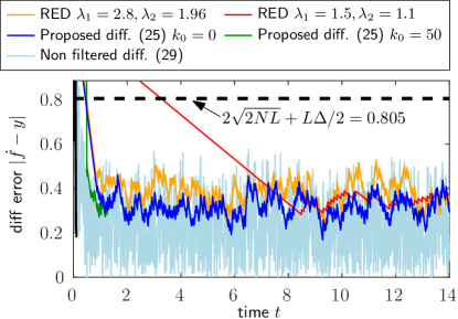
Figure 1: Simulation results with sampling time $\Delta=0.01$, comparing the RED, the non-filtered differentiator in (26) and the proposed differentiator (25) with $L=1,N=0.08$, using $k_{0}=0$ and $k_{0}=50$. The plots show the differentiation error $|\dot{f}-y|$ in each case.

VI Conclusions

A first-order exact differentiator that guarantees optimal worst-case accuracy in a fixed time while being robust to measurement noise and having Lipschitz continuous output was introduced. The latter combination of properties makes this differentiator unique in comparison with other existing differentiators. The fact that the differentiator is exact means that its output converges to the true derivative in the absence of measurement noise. The maximum Lipschitz constant of the differentiator’s output is a tunable parameter that allows to trade convergence rate for “smoothness”: the higher this constant, the faster the convergence but the more “noisy” the output. Both continuous-time and sample-based versions of the differentiator are developed, the latter being the digitally implementable one. The theoretical guarantees are given for both differentiator versions.

Appendix A Auxiliary lemmata

Lemma 3.

[8, Adapted from Lemmas 5.7 and 5.8] Let $L\geq 0$, suppose that $u\in\mathcal{U}$, and consider a fixed $t>0$ such that $\hat{N}(t)=0$ with $\hat{N}(t)$ defined in (7). Let $\mu\in(0,t]$ and suppose $Q$ as defined in (7d) satisfies

$$|Q(t,T,\sigma)|\leq\frac{L\sigma(T-\sigma)}{2}$$ (34)

for all $T\in(0,\mu]$ and all $\sigma\in[0,T]$. Then, the limit $\beta:=\lim_{T\to 0^{+}}(u(t)-u(t-T))/T$ exists. Moreover,

$$|u(t-{\sigma})-u(t)+\beta{\sigma}|\leq\frac{L{\sigma}^{2}}{2}$$ (35)

holds for all $\sigma\in[0,\mu]$.

Lemma 4.

[8, Lemma 5.9] Let $L,\hat{N}>0,\hat{T}\geq 2\sqrt{\hat{N}/L},u\in\mathcal{U}$. Let $\beta:=(u(t)-u(t-\hat{T}))/\hat{T}$ and suppose

$$|Q(t,\hat{\sigma},\hat{T})|\leq 2\hat{N}+\frac{L\hat{T}(\hat{\sigma}-\hat{T})}{2}$$ (36)

if fulfilled for some $\hat{\sigma}\in[\hat{T},t]$. Then, (35) holds for $\sigma=\hat{\sigma}$.

Lemma 5.

[8, Lemma 4.1] Let $L\geq 0,f\in\mathcal{F}_{L}$. Then,

$$|f(t-\sigma)-f(t)+\dot{f}(t)\sigma|\leq\frac{L\sigma^{2}}{2}$$ (37)

holds for all $t\geq 0$ and all $\sigma\in[0,t]$.

Appendix B Proofs of all Lemmata

Proof of Lemma 1.

For $t\geq\sqrt{2N/L}$, the result follows from [8, Theorem 5.1]. Now, consider $t\in(0,\sqrt{2N/L})$. Note that $\hat{T}(t)=\overline{T}$ leads to the contradiction $t\geq\hat{T}(t)=\overline{T}=\sqrt{2\overline{N}/L}\geq\sqrt{2N/L}$ and for $\hat{T}(t)=t$ the result follows from [8, Lemma 5.4]. Distinguish two remaining cases as i) $\hat{T}(t)=0$ and ii) $\hat{T}(t)=2\sqrt{\hat{N}(t)/L}\in(0,t)$. For these cases, we show that (35) holds for $\sigma=t$ with $\beta=y_{\mathrm{w}}(t)$.

Case i) implies $\hat{N}(t)=0$ which in turn implies that (34) is fulfilled for all $T\in(0,\mu],\sigma\in[0,T]$ and $\mu=\min\{t,\overline{T}\}=t$ due to (7c). Applying Lemma 3 with $\mu=t$, it follows that $y_{\mathrm{w}}(t)=\beta$ and that (35) holds for ${\sigma}=t$.

In case ii), $\hat{T}(t)\in(0,t)$ and (36) is fulfilled for $\hat{\sigma}=t$, $\hat{N}=\hat{N}(t)$, $\hat{T}=\hat{T}(t)$ due to the construction of $\hat{N}(t)$ in (7c) (see [8, Remark 5.10]). Thus, applying Lemma 4 yields that (35) holds for ${\sigma}=t$ with $\beta=y_{\mathrm{w}}(t)$.

In both cases, $|f(0)-f(t)+y_{\mathrm{w}}(t)t|\leq\frac{Lt^{2}}{2}+2N$ is obtained due to $|\eta(t)|\leq N$. Combine this inequality with (37) from Lemma 5, setting $\sigma=t$, to obtain $|y_{\mathrm{w}}(t)t-\dot{f}(t)t|\leq Lt^{2}+2N.$ Division by $t$ proves the claim. ∎

Proof of Lemma 2.

The case $k\Delta\geq\sqrt{2N/L}$ follows from [8, Theorem 7.1]. In the other case, $\hat{\ell}_{k}=k$ allows to apply [8, Lemma 5.4] with $\hat{T}=\Delta\hat{\ell}_{k}$, and $\hat{\ell}_{k}=\overline{k}$ implies the contradiction $\overline{k}\Delta\leq k\Delta<\sqrt{2N/L}\leq\sqrt{2\overline{N}/L}=(\overline{k}-1)\Delta$. The remaining case is $\hat{\ell}_{k}=\left\lceil\frac{2}{\Delta}\sqrt{\frac{\hat{N}_{k}}{L}}\right\rceil\in[1,k)$. In that case, apply Lemma 4 with $t=\hat{\sigma}=k\Delta$, $\hat{T}=\hat{\ell}_{k}\Delta$ while noting that $|Q(k\Delta,k\Delta,\hat{\ell}_{k}\Delta)|=|Q_{k,k,\hat{\ell}_{k}}|\leq 2\hat{N}_{k}+L\Delta^{2}\hat{\ell}_{k}(k-\hat{\ell}_{k})/2$ is fulfilled due to (26d), (7d), and (26c). That lemma yields $|u_{0}-u_{k}+\beta k\Delta|\leq Lk^{2}\Delta^{2}/2$ with $\beta=y_{\mathrm{s},k}$, implying $|f_{0}-f_{k}+y_{\mathrm{s},k}k\Delta|\leq Lk^{2}\Delta^{2}/2+2N$ due to $|\eta_{k}|\leq N$ and yielding $|y_{\mathrm{s},k}k\Delta-\dot{f}(k\Delta)k\Delta|\leq Lk^{2}\Delta^{2}+2N$ after combining with the statement of Lemma 5. Finally, divide by $k\Delta$. ∎

References

- [1] L. Fraguela, M. T. Angulo, J. A. Moreno, and L. Fridman, “Design of a prescribed convergence time uniform Robust Exact Observer in the presence of measurement noise,” in Proc. IEEE Conf. on Decis. and Control, 2012, pp. 6615–6620.
- [2] L. K. Vasiljevic and H. K. Khalil, “Differentiation with high-gain observers the presence of measurement noise,” in Conference on Decision and Control. IEEE, 2006, pp. 4717–4722.
- [3] J. Holloway and M. Krstic, “Prescribed-time observers for linear systems in observer canonical form,” IEEE Trans. Autom. Control, vol. 64, no. 9, pp. 3905–3912, 2019.
- [4] Y. Orlov, R. I. Verdes Kairuz, and L. T. Aguilar, “Prescribed-Time Robust Differentiator Design Using Finite Varying Gains,” IEEE Control Syst. Lett., vol. 6, pp. 620–625, 2022.
- [5] A. Levant, “Robust Exact Differentiation via Sliding Mode Technique,” Automatica, vol. 34, no. 3, pp. 379–384, 1998.
- [6] E. Cruz-Zavala, J. A. Moreno, and L. M. Fridman, “Uniform robust exact differentiator,” IEEE Trans. Autom. Control, vol. 56, no. 11, pp. 2727–2733, 2011.
- [7] R. Seeber, H. Haimovich, M. Horn, L. M. Fridman, and H. De Battista, “Robust exact differentiators with predefined convergence time,” Automatica, vol. 134, p. 109858, 2021.
- [8] R. Seeber and H. Haimovich, “Optimal robust exact differentiation via linear adaptive techniques,” Automatica, vol. 148, p. 110725, 2023.
- [9] R. Aldana-López, R. Seeber, H. Haimovich, and D. Gómez-Gutiérrez, “On inherent limitations in robustness and performance for a class of prescribed-time algorithms,” Automatica, vol. 158, p. 111284, 2023.
- [10] R. Seeber, “Worst-case error bounds for the super-twisting differentiator in presence of measurement noise,” Automatica, vol. 152, p. 110983, 2023.
- [11] J. A. Moreno, “Arbitrary-order fixed-time differentiators,” IEEE Trans. Autom. Control, vol. 67, no. 3, pp. 1543–1549, 2021.
- [12] R. Aldana-López, R. Seeber, D. Gómez-Gutiérrez, M. T. Angulo, and M. Defoort, “A redesign methodology generating predefined-time differentiators with bounded time-varying gains,” International Journal of Robust and Nonlinear Control, vol. 33, no. 15, pp. 9050–9065, 2023.
- [13] S. Diop, J. Grizzle, and F. Chaplais, “On numerical differentiation algorithms for nonlinear estimation,” in Proceedings of the 39th IEEE Conference on Decision and Control (Cat. No. 00CH37187), vol. 2. IEEE, 2000, pp. 1133–1138.
- [14] A. Levant, “Finite differences in homogeneous discontinuous control,” IEEE Trans. Autom. Control, vol. 52, no. 7, pp. 1208–1217, 2007.
- [15] ——, “Chattering analysis,” IEEE Trans. Autom. Control, vol. 55, no. 6, pp. 1380–1389, 2010.
- [16] V. Utkin, “Discussion aspects of high-order sliding mode control,” IEEE Trans. Autom. Control, vol. 61, no. 3, pp. 829–833, 2015.
- [17] H. Haimovich, R. Seeber, R. Aldana-López, and D. Gómez-Gutiérrez, “Differentiator for noisy sampled signals with best worst-case accuracy,” IEEE Control Systems Letters, vol. 6, pp. 938–943, 2021.
- [18] B. Brogliato and A. Polyakov, “Digital implementation of sliding-mode control via the implicit method: A tutorial,” International Journal of Robust and Nonlinear Control, vol. 31, no. 9, pp. 3528–3586, 2021.
- [19] J. E. Carvajal-Rubio, J. D. Sánchez-Torres, M. Defoort, M. Djemai, and A. G. Loukianov, “Implicit and explicit discrete-time realizations of homogeneous differentiators,” International Journal of Robust and Nonlinear Control, vol. 31, no. 9, pp. 3606–3630, 2021.
- [20] A. Hanan, A. Levant, and A. Jbara, “Low-chattering discretization of homogeneous differentiators,” IEEE Trans. Autom. Control, vol. 67, no. 6, pp. 2946–2956, 2021.
- [21] R. Aldana-López, R. Seeber, H. Haimovich, and D. Gómez-Gutiérrez, “Exact differentiator with Lipschitz continuous output and optimal worst-case accuracy under bounded noise,” in 2023 62nd IEEE Conference on Decision and Control (CDC). IEEE, 2023, pp. 7874–7880.
- [22] A. F. Filippov, Differential equations with discontinuous righthand sides, ser. Mathematics and its Applications (Soviet Series). Dordrecht: Kluwer Academic Publishers Group, 1988, vol. 18, translated from the Russian.