Entanglement entropy in lattices with non-abelian gauge groups

Abstract

Entanglement entropy, taken here to be geometric, requires a geometrically separable Hilbert space. In lattice gauge theories, it is not immediately clear if the physical Hilbert space is geometrically separable. In a previous paper we have shown that the physical Hilbert space in pure gauge abelian lattice theories exhibits some form of geometric scaling with the lattice volume, which suggest that the space is locally factorizable and, therefore, geometrically separable. In this paper, we provide strong evidence that indicates that this scaling is not present when the group is non-abelian. We do so by looking at the scaling of the dimension of the physical Hilbert space of theories with certain discrete groups. The lack of an appropriate scaling implies that the physical Hilbert space of such a theory does not admit a local factorization. We then extend the reasoning, as sensibly possible, to $SU(2)$ and $SU(N)$ to reach the same conclusion. Lastly, we show that the addition of matter fields to non-abelian lattice gauge theories makes the resulting physical Hilbert space locally factorizable.

I Introduction

There has been considerable debate Buividovich and Polikarpov (2008); Casini et al. (2014); Aoki et al. (2015); Radicevic (2014); Donnelly (2012); Ghosh et al. (2015); Lin and Radicevic (2020) about how entanglement entropy can be defined in the context of lattice gauge theories. This stems from difficulties in reasoning about the physical Hilbert space of such theories when seen through the lens of a constrained unphysical space. For example, the unphysical Hilbert space of a pure lattice gauge theory is the space of group-valued degrees of freedom (d.o.f.) on the links of a lattice. However, constraining the unphysical space in order to obtain the physical one leads to a physical Hilbert space of lower dimension, and, consequently, fewer d.o.f.. It follows that there would not be enough physical d.o.f. for every link in the lattice and one must think of the physical d.o.f. as being associated with different geometrical objects if they are to remain on the same lattice. In two spatial dimensions and when the gauge group is abelian, the objects with which physical d.o.f. are associated are the plaquettes. Of course, one does not simply make that choice. Instead, one looks at how the physical Hilbert space scales with the lattice size, typically using discrete groups, and finds that this scaling depends only on the number of plaquettes (see Fig. 1). With this ansatz, one can derive the precise algebra and form of the physical space. A natural question then arises: does this general scheme also apply to non-abelian theories? For pure gauge theories, this paper shows that the answer is negative. Nonetheless, when matter fields are introduced, the non-commutativity of the group elements becomes irrelevant, thus allowing for a similar factorization to what is possible with abelian gauge groups when coupled with matter.

II An overview of the problem

In order to straightforwardly define an entanglement entropy in a quantum theory, it is generally necessary for the Hilbert space of the theory to exhibit a tensor product structure such that the total space can be expressed as a tensor product of local Hilbert spaces Lin and Radicevic (2020); Ghosh et al. (2015); Aoki et al. (2015) The local Hilbert spaces form the local d.o.f. of the theory. Naively, this appears to be the case for lattice theories, in which space is discretized and fields are associated with lattice objects, such as vertices, links, plaquettes, etc.. In pure gauge Kogut-Susskind Hamiltonian lattice theories Kogut and Susskind (1975), one starts with unphysical gauge fields having local unphysical Hilbert spaces associated with links in the lattice. Gauge constraints are then imposed on the total unphysical Hilbert space to obtain the physical Hilbert space as a subspace of the unphysical space. It is generally clear that one cannot construct an isomorphism between the unphysical and physical spaces on a finite and discrete lattice with discrete groups, since the physical space is a strict subspace of the unphysical one.

What is less obvious is that, when imposing the specific constraints of gauge theory, one also cannot generally construct an isomorphism between the set of unphysical local Hilbert spaces and the set of physical ones. In other words, the physical space will have fewer d.o.f. than the unphysical space. This can be seen easily if one works with a $Z_{2}$ gauge group, which results in local Hilbert spaces of dimension $2$, the minimally viable dimension of what could be considered a d.o.f.. Any reduction in the dimension of the total Hilbert space then implies that the number of d.o.f. must decrease. The immediate implication is that local physical spaces, if they exist at all, cannot generally be associated with the same lattice objects as the unphysical ones on a finite lattice. A necessary condition for the local physical Hilbert spaces to exist is for the dimension of the physical Hilbert space to scale appropriately with lattice size. Conversely, a lack of such scaling implies that the total Hilbert space cannot be factored into local Hilbert spaces. We will use this to show the impossibility of having local physical Hilbert spaces in certain non-abelian pure gauge lattice theories.

Figure 1: Illustration of the scaling of the physical Hilbert space in abelian theories with discrete groups on lattices in two spatial dimensions. Both lattices have the same number of plaquettes, but lattice (a) has 13 links, whereas lattice (b) has 12 links. It can be shown that the physical Hilbert space of both lattices has the same dimension.

Before moving to the more general lattice problem and entanglement entropy, it may be useful to look at some simple systems to illustrate some of the abstract points above, as well as to provide a brief overview of some of the more significant Hilbert space factorization issues found in literature. We use this opportunity to introduce some notation, as well as terminology and basic assumptions. We start with a quantum system whose physical space is described by a single quantum spin. That is, the physical Hilbert space of this system, $\mathcal{H}^{1}$, is the space of vectors of the form

$$\ket{\psi}=\alpha\ket{\uparrow}+\beta\ket{\downarrow}.$$ (1)

A generating set for the von Neumann algebra of this Hilbert space is

$$\mathcal{S}=\{I,\sigma^{z},\sigma^{x}\}.$$ (2)

That is, the von Neumann algebra of the Hilbert space is the smallest von Neumann algebra containing $\mathcal{S}$, and we write this algebra as $\mathcal{A}(\mathcal{S})$. The operator $I$ is the identity operator, while $\sigma^{z}$ and $\sigma^{x}$ are the familiar Pauli operators satisfying $\sigma^{z}\ket{\uparrow}=\ket{\uparrow},\sigma^{z}\ket{\downarrow}=-\ket{\downarrow}$, $\sigma^{x}\ket{\uparrow}=\ket{\downarrow}$, and $\sigma^{x}\ket{\downarrow}=\ket{\uparrow}$. However, for consistency with lattice notation and clarity, we will relabel the operators as $U\equiv\sigma^{x}$ and $L\equiv\sigma^{z}$. The operators $L$ and $U$ are reminiscent here of canonical variables in the sense that they can be used to completely describe the state of the local system at a given time. With that understanding, we will call them canonical pairs. The algebra generated by canonical pairs, together with the identity operator, cannot be factored into a tensor product of algebras. We will use the term local algebra for such an algebra, which is generated by a maximal set of linearly independent non-commuting operators, together with the identity, and which cannot be factored. A local algebra, together with the local Hilbert space it acts on, is colloquially termed degree of freedom (d.o.f.). For simplicity, we will consider the identity operator as implied when referring to generating sets. An algebraic factor, and therefore a local algebra, satisfies $\mathcal{A}\cap\mathcal{A}^{\prime}=\{cI\}$, where $\mathcal{A}^{\prime}$ is the commutant of $\mathcal{A}$ (the set of all operators that commute with all operators in $\mathcal{A}$) and $c$ is an arbitrary constant. The set $\mathcal{A}\cap\mathcal{A}^{\prime}=Z_{\mathcal{A}}$ is called the center of $\mathcal{A}$. Algebras that satisfy $Z_{\mathcal{A}}=\{cI\}$ are said to have a trivial center and are factors. Local algebras, as defined above, are factors by construction.

We can, at this point, consider a larger system, which is formed by taking the direct product of two single spin spaces, $\mathcal{H}^{2}=\mathcal{H}^{1}_{L}\otimes\mathcal{H}^{1}_{R}$, where the subscripts L and R are used to distinguish the two subspaces. The most general state on this space takes the form

$$\ket{\psi}_{LR}=\alpha\ket{\uparrow_{L}\uparrow_{R}}+\beta\ket{\uparrow_{L}\downarrow_{R}}+\delta\ket{\downarrow_{L}\uparrow_{R}}+\gamma\ket{\downarrow_{L}\downarrow_{R}},$$ (3)

with the standard normalization condition $\alpha^{2}+\beta^{2}+\delta^{2}+\gamma^{2}=1$.

A set of local algebras for this space is $\mathcal{A}^{1}_{L}=\mathcal{A}(\{L_{L}\otimes I_{R},U_{L}\otimes I_{R}\})\equiv\mathcal{A}(\{L_{L},U_{L}\})$ , $\mathcal{A}^{1}_{R}=\mathcal{A}(\{L_{R},U_{R}\})$, and we omit the multiplication with the identity where it can be inferred from the context. This decomposition is only unique up to unitary equivalence, and since all Hilbert spaces of the same finite dimension are unitarily equivalent, the relevant quantity here is the dimension of $\mathcal{H}^{2}$. The total algebra of the system $\mathcal{A}^{2}$ is the closure of the local algebras or the smallest von Neumann algebra that contains both $\mathcal{A}^{1}_{L}$ and $\mathcal{A}^{1}_{R}$, and we write $\mathcal{A}^{2}=\mathcal{A}^{1}_{R}\otimes\mathcal{A}^{1}_{L}$. The existence of a tensor product factorization of $\mathcal{H}^{2}$ or of a factorization of $\mathcal{A}^{2}$ do not imply that all subalgebras of $\mathcal{A}^{2}$ have trivial centers. Conversely, the existence of algebras with a non-trivial center does not preclude a factorization of the Hilbert space or the algebra. For example, the Hilbert space $\mathcal{H}^{2}$ can be factorized by construction (i.e., it is a tensor product of two Hilbert spaces). However, the algebra

$$\mathcal{A}_{Z}=\mathcal{A}(\{L_{L},U_{L},L_{R}\}),$$ (4)

which is a subalgebra of $\mathcal{A}^{2}$, has a non-trivial center since $\mathcal{A}_{Z}^{\prime}=\mathcal{A}(\{L_{R}\})$ and, therefore, $\mathcal{A}_{Z}\cap\mathcal{A}_{Z}^{\prime}=\{cL_{R}\}$. Even simpler, all algebras of the form $\mathcal{A}(\{A\})$ have a non-trivial center for some operator $A$ not proportional to the identity.

The space $\mathcal{H}^{2}$ is the same space as the unphysical Hilbert space of a pure gauge $Z_{2}$ $1+1$ dimensional Kogut-Susskind Hamiltonian lattice with two links. In the gauge theory, one imposes a gauge constraint that restricts the physical states to states of the form

$$\ket{\psi}_{LR}^{{}^{\text{phys.}}}=\alpha\ket{\uparrow\uparrow}+\beta\ket{\downarrow\downarrow},$$ (5)

where we omitted some of the L and R subscripts. The dimension of the resulting physical Hilbert space, which we denote by $\mathcal{H}^{2}_{{}^{\text{phys.}}}$, is now the same as that of $\mathcal{H}^{1}$. The physical Hilbert space has only one d.o.f. and this d.o.f. cannot be meaningfully assigned to the two links in the lattice. The gauge constraints act as a cutoff, leading to a change in scale. Imposing the constraint that all states take the form in Eq. (5) means that some operators in the initial algebra become unphysical, in the sense that they do not preserve this form. For example:

$$U_{L}(\alpha\ket{\uparrow\uparrow}+\beta\ket{\downarrow\downarrow})=\alpha\ket{\downarrow\uparrow}+\beta\ket{\uparrow\downarrow}.$$ (6)

The operators in $\mathcal{A}^{2}$ that preserve the physical form of states are generated by the set $S^{2}_{{}^{\text{phys.}}}=\{L_{L},L_{R},U_{L}U_{R}\}$. The operators in $\mathcal{A}(S^{2}_{{}^{\text{phys.}}})$ are called physical operators. The operators $L_{L}$ and $L_{R}$ are only distinct when they act on unphysical states. For any physical state $\ket{\psi}_{LR}^{{}^{\text{phys.}}}$, $L_{L}\ket{\psi}_{LR}^{{}^{\text{phys.}}}=L_{R}\ket{\psi}_{LR}^{{}^{\text{phys.}}}$, and we write $L_{L}\mathrel{\overset{\makebox[0.0pt]{\mbox{\tiny P}}}{=}}L_{R}$. To be clear, if we postulate that the physical world consists of only physical or gauge invariant states, the operators $L_{L}$ and $L_{R}$ are the same matrix (i.e., they are the same operator). This highlights an important aspect: certain statements about operators in $\mathcal{A}(S^{2}_{{}^{\text{phys.}}})$ are different when the operators act on the unphysical Hilbert space from when they act on the physical subspace. Furthermore, the physical algebra cannot resolve more details than can be distinguished through the physical Hilbert space. In other words, the subset of operators in $\mathcal{A}^{2}$ that are physical cannot create or measure more states than are available in the physical Hilbert space. That is, there is no L and R in $\mathcal{H}^{2}_{{}^{\text{phys.}}}$, no more more than there would be in $\mathcal{H}^{1}$. We, again, arrive at the idea that the dimension of the physical Hilbert space is a significant quantity.

Figure 2: A two plaquette lattice. The numbers label the links.

A more pertinent example to lattice gauge theory is the two-plaquette $2+1$ dimensional $Z_{2}$ pure gauge lattice, shown in Fig. 2. The unphysical Hilbert space of this theory associates a $Z_{2}$ element, which is equivalent to a basis of $\mathcal{H}^{1}$, to every link in the lattice. The total unphysical Hilbert space is a tensor product of $\mathcal{H}^{1}$ spaces: $\mathcal{H}^{7}=\mathcal{H}^{1}_{1}\otimes\ldots\otimes\mathcal{H}^{1}_{7}$, where the subscripts label the local spaces and correspond to the numbering of the links in Fig. 2. One can, at this point, proceed to (partially) fix the gauge using a variation of maximal tree gauge fixing Creutz (1983) by fixing a set of links to a certain vector (e.g., $\ket{\uparrow}$) as long as the fixed links do not form any loops. This has the effect of reducing the dimension of the unphysical Hilbert space, from $\dim(\mathcal{H}^{7})=2^{7}$ to anything of the form $\dim(\mathcal{H})=2^{n},$ with $n\in\{2,\ldots,6\}$, the lower bound being the dimension of the physical space, obtained when a maximal set of links has been fixed. The physical space is isomorphic to $\mathcal{H}^{2}$, which is a well known duality Wegner (1971). The physical states are of the form

$$\ket{\psi}_{7}^{{}^{\text{phys.}}}=\alpha\ket{\uparrow\uparrow\uparrow\uparrow\uparrow\uparrow\uparrow}+\beta\ket{\downarrow\downarrow\downarrow\uparrow\uparrow\uparrow\downarrow}+\gamma\ket{\uparrow\uparrow\uparrow\downarrow\downarrow\downarrow\uparrow}+\delta\ket{\uparrow\uparrow\uparrow\uparrow\uparrow\uparrow\downarrow},$$ (7)

and we can identify the unphysical basis as the basis of electric fluxes through links. A more illuminating way of writing the physical states is

$$\ket{\psi}_{7}^{{}^{\text{phys.}}}=\alpha\ket{\vbox{\hbox{\includegraphics[height=6.45831pt]{symb/dplaq0000000}}}}+\beta\ket{\vbox{\hbox{\includegraphics[height=6.45831pt]{symb/dplaq1111000}}}}+\gamma\ket{\vbox{\hbox{\includegraphics[height=6.45831pt]{symb/dplaq0001111}}}}+\delta\ket{\vbox{\hbox{\includegraphics[height=6.45831pt]{symb/dplaq1110111}}}},$$ (8)

where the thick lines correspond to $\ket{\downarrow}$ states on the respective links. We can see that the space of physical states is isomorphic to an $\mathcal{H}^{2}$ space with $\ket{\vbox{\hbox{\includegraphics[height=6.45831pt]{symb/dplaq0000000}}}}=\ket{\uparrow\uparrow},\ket{\vbox{\hbox{\includegraphics[height=6.45831pt]{symb/dplaq1111000}}}}=\ket{\downarrow\uparrow},\ket{\vbox{\hbox{\includegraphics[height=6.45831pt]{symb/dplaq0001111}}}}=\ket{\uparrow\downarrow}$, and $\ket{\vbox{\hbox{\includegraphics[height=6.45831pt]{symb/dplaq1110111}}}}=\ket{\downarrow\downarrow}$. A relevant observation is that we cannot associate the two $\mathcal{H}^{1}$ factors of $\mathcal{H}^{2}$ with links in the lattice in any sort of uniform way. Once again, gauge constrains act as a cutoff that requires a (slight) change of scale. If one proceeds to investigate the physical Hilbert space of larger lattices with the same group (and with free boundary conditions), one finds that the physical Hilbert space has dimension $\dim(\mathcal{H}_{{}^{\text{phys.}}})=2^{n}$, where $n$ is the number of plaquettes in the lattice. It is then natural to interpret the physical d.o.f. as fluxes through plaquettes rather than through links.

In terms of algebras, the unphysical algebra can be written as $\mathcal{A}^{7}=\mathcal{A}^{1}_{1}\otimes\ldots\otimes\mathcal{A}^{1}_{7}$, where the subscripts label the links. The subset of operators of $\mathcal{A}^{7}$ that are physical is generated by

$$S^{7}_{{}^{\text{phys.}}}=\{L_{i},U_{1}U_{2}U_{3}U_{7},U_{1}U_{2}U_{3}U_{7}\},$$ (9)

where $i\in\{1,\ldots,7\}$. However, as was the case before, $S^{7}_{{}^{\text{phys.}}}$ contains redundancies such as

$$L_{1} \mathrel{\overset{\makebox[0.0pt]{\mbox{\tiny P}}}{=}}L_{2}\mathrel{\overset{\makebox[0.0pt]{\mbox{\tiny P}}}{=}}L_{3},$$

$$L_{4} \mathrel{\overset{\makebox[0.0pt]{\mbox{\tiny P}}}{=}}L_{5}\mathrel{\overset{\makebox[0.0pt]{\mbox{\tiny P}}}{=}}L_{6},$$

$$L_{7} \mathrel{\overset{\makebox[0.0pt]{\mbox{\tiny P}}}{=}}L_{3}L_{4}.$$ (10)

From an algebraic perspective, the question is whether $\mathcal{A}(S^{7}_{{}^{\text{phys.}}})$ can be factored, and if so, how. The problem is typically Buividovich and Polikarpov (2008); Casini et al. (2014) approached by attempting to assign the operators in $S^{7}_{{}^{\text{phys.}}}$ into two sets, one for each of the left and right sides of the lattice. This can naively run into a number of issues. Specifically, Buividovich and Polikarpov (2008) attempts to factor operators such as $U_{1}U_{2}U_{3}U_{7}$ into $U_{1}U_{2}U_{3}I_{7}$ and $I_{1}I_{2}I_{3}U_{7}$, with $I_{n}$ being identity operators on the respective subspaces, noting that the factored operators cease to act exclusively in the physical subspace (i.e., they are not gauge invariant). A slightly different attempt is made in Casini et al. (2014), which notes operator identities similar to those in Eq. (II) and concludes that a choice of algebra such as $\mathcal{A}_{EC}=\mathcal{A}(\{L_{3},L_{4},L_{7},U_{4}U_{5}U_{6}U_{7}\})$ has $L_{4}$ as a center, since $L_{4}$ commutes with all other operators in $\mathcal{A}_{EC}$. This is indeed the case, as it was the case with Eq. (4). However, this does not imply that all factorization choices result in algebras with center. Specifically, $\mathcal{A}_{L}=\mathcal{A}(\{L_{3},U_{1}U_{2}U_{3}U_{7}\})$ and $\mathcal{A}_{R}=\mathcal{A}(\{L_{4},U_{4}U_{5}U_{6}U_{7}\})$ are both factors and satisfy $\mathcal{A}(S^{7}_{{}^{\text{phys.}}})=\mathcal{A}_{L}\otimes\mathcal{A}_{R}$. Consequently, we can relabel the generating set operators as $L_{A}\equiv L_{3},U_{L}\equiv U_{1}U_{2}U_{3}U_{7},L_{B}\equiv L_{4},$ and $U_{R}=U_{4}U_{5}U_{6}U_{7}$ such that the subalgebras can now be written as $\mathcal{A}_{L}=\mathcal{A}(\{L_{L},U_{L}\}),\mathcal{A}_{R}=\mathcal{A}(\{L_{R},U_{R}\})$, which matches what one would expect by looking at the dimension of the physical Hilbert space.

The change in geometry resulting from the reduction in the dimension of the Hilbert space has additional implications to the locality of operators: local operators in the physical space are not necessarily local in the unphysical space nor are unphysical operators necessarily local in the physical space. For example, in the two plaquette lattice, $L_{7}\mathrel{\overset{\makebox[0.0pt]{\mbox{\tiny P}}}{=}}L_{L}L_{R}$ and $U_{L}=U_{1}U_{2}U_{3}U_{7}$. Both of these equivalences represent matrix expressions and, without further constraints, the only meaningful measure of locality is the form that a particular matrix takes in a given basis. A more meaningful notion of locality arises when dynamics are introduced through a Hamiltonian. If the theory being modeled is one that is expected to approximate physical reality, then this Hamiltonian should be such that correlations do not violate causality, which usually implies that the terms in the Hamiltonian are, by construction, local. One may take things a step further by noting that it is the dynamics that give the underlying Hilbert space a topology. In more specific but perhaps less general terms, the topology and geometry of the space are fully given by the way that rays of light propagate and the propagation of rays of light is governed by dynamics. The relevance to geometric entanglement entropy and Hilbert space tensor product structures is that one must be careful when using the locality of operators as a fundamental assumption, especially when constraints are involved or when used with theories that are not causal.

II.1 Entanglement Entropy and Unphysical Hilbert Spaces

Entanglement entropy gives a quantitative measure of the extent to which parts of a state belonging to complementary subspaces of a Hilbert space are correlated. But physical states in gauge theories, whose Hilbert spaces are defined as subspaces of unphysical/extended Hilbert spaces, can appear as entangled states in the unphysical space. For example, the state with $\alpha=\beta=1/\sqrt{2}$ in Eq. (5) is a Bell pair with perfect entanglement despite the physical space being that of a single spin, for which the notion of entanglement seems absurd. There exist arguments Donnelly (2012); Buividovich and Polikarpov (2008) in literature that suggest that such entanglement is indeed a legitimate physical phenomenon. In particular, for states of the form found in Eq. (5), one finds that

$$S_{1}^{\prime} =-\operatorname{tr}\rho_{1}\log\rho_{1}=-\alpha^{2}\log\alpha^{2}-\beta^{2}\log\beta^{2},$$ (11)

which is Donnelly (2012) a classical Shannon entropy term of the distribution of basis vectors and where

$$\rho_{1} =\operatorname{tr}_{2}\left[\alpha^{2}\ket{\uparrow}_{1}\otimes\ket{\uparrow}_{2}\bra{\uparrow}_{2}\otimes\bra{\uparrow}_{1}+\beta^{2}\ket{\downarrow}_{1}\otimes\ket{\downarrow}_{2}\bra{\downarrow}_{2}\otimes\bra{\downarrow}_{1}+\cdots\right]$$

$$=\alpha^{2}\ket{\uparrow}_{1}\bra{\uparrow}_{1}+\beta^{2}\ket{\downarrow}_{1}\bra{\downarrow}_{1}$$ (12)

is the reduced density matrix.

The need to use unphysical Hilbert spaces to calculate the entanglement entropy stems from the assumption that it is impossible to partition the physical Hilbert space of lattice gauge theories, an assumption that we have shown Hategan (2018) to be unnecessary in $2+1$ dimensional abelian pure gauge theories (briefly illustrated in the previous section) and in abelian gauge theories when coupled with matter fields. Furthermore, if we assume that the physical Hilbert space is the only accurate representation of physical reality, an entanglement entropy calculated on an extended Hilbert space can only be valid to the extent that it leads to the same result on any extended Hilbert space that starts from the physical space, similar to how the outcome of renormalization does not depend on the details of the renormalization scheme. However, this is clearly not so with entanglement entropy as we will show in the following paragraphs.

With Eq. (5), which we repeat here for clarity, we chose to extend the physical Hilbert space such that physical states are of the form

$$\ket{\psi}_{LR}^{{}^{\text{phys.}}}=\alpha\ket{\uparrow\uparrow}+\beta\ket{\downarrow\downarrow}.$$ (13)

Since there is no physics that can constrain the construction of the unphysical space, this is simply a choice of two orthogonal vectors in a two-spin space. Consequently, we could have chosen the unphysical space such that physical states are of the form

$$\ket{\psi^{\prime\prime}}=\dfrac{\alpha}{\sqrt{2}}\big{(}\ket{\uparrow\uparrow}+\ket{\downarrow\downarrow}\big{)}+\dfrac{\beta}{\sqrt{2}}\big{(}\ket{\uparrow\uparrow}-\ket{\downarrow\downarrow}\big{)},$$ (14)

for which we would obtain

$$S_{1}^{\prime\prime}=-\dfrac{(\alpha+\beta)^{2}}{2}\log\dfrac{(\alpha+\beta)^{2}}{2}-\dfrac{(\alpha-\beta)^{2}}{2}\log\dfrac{(\alpha-\beta)^{2}}{2}.$$ (15)

We recognize Eq. (15) as similar to a momentum-space version of Eq. (13) and, if the spins in Eq. (13) were associated with different physical regions of space, there would be a preferential geometrical basis that would favor Eq. (13) or a local unitary transformation of it which would preserve the entanglement entropy. However the fact that Eq. (13) and Eq. (15) are related by a unitary transformation that acts exclusively in an unphysical subspace, one cannot use physical arguments to elevate one choice above the other.

The example physical Hilbert space in Eq. (13) can be extended in ways that can lead to arbitrarily parameterized entanglement entropies:

$$\ket{\psi^{\prime\prime}}=\alpha\big{(}\gamma\ket{\uparrow\uparrow}_{1}\otimes\ket{\uparrow\uparrow}_{2}+\delta\ket{\downarrow\downarrow}_{1}\otimes\ket{\downarrow\downarrow}_{2}\big{)}+\beta\big{(}\gamma\ket{\uparrow\downarrow}_{1}\otimes\ket{\uparrow\downarrow}_{2}+\delta\ket{\downarrow\uparrow}_{1}\otimes\ket{\downarrow\uparrow}_{2}\big{)},$$ (16)

with an entanglement entropy of

$$S_{1}^{\prime\prime} =-\alpha^{2}\gamma^{2}\log\alpha^{2}\gamma^{2}-\alpha^{2}\delta^{2}\log\alpha^{2}\delta^{2}-\beta^{2}\gamma^{2}\log\beta^{2}\gamma^{2}-\beta^{2}\delta^{2}\log\beta^{2}\delta^{2}$$

$$=-\alpha^{2}\log\alpha^{2}-\beta^{2}\log\beta^{2}-\gamma^{2}\log\gamma^{2}-\delta^{2}\log\delta^{2},$$ (17)

where $\gamma$ can be varied arbitrarily, up to normalization.

Buividovich and Polikarpov Buividovich and Polikarpov (2008) argue that a “minimal” extension of the Hilbert space is justified. However, it is unclear what “minimal” means and whether it can lead to an unambiguous solution. If “minimal” refers to the dimension of the extended Hilbert space, then it does not unambiguously specify a solution, as evidenced by Eq. (14) and Eq. (15).

These arguments suggest that unphysical Hilbert spaces are unsuitable in defining an entanglement entropy, since the results depend on the choice of unphysical space and cannot be falsified. This work takes as fundamental the assumption that either a definition of entanglement entropy be based exclusively on physical aspects of the theory or that the definition is such that unphysical aspects can be removed from the final result. Nonetheless, when discussing field theories, and, in particular, lattice theories, it is not always clear that this is possible, for reasons that we will outline shortly.

II.2 Geometric Entanglement Entropy and Lattice Theories

Until this point in the discussion, we focused mostly on a generic form of Entanglement Entropy, which applies to any bipartition of the Hilbert space, giving little weight to the geometry of the underlying space. However, we are often interested in geometric entanglement entropy, which implies a geometric bipartition of the Hilbert space in which each subspace belongs to a well defined geometric region. In order to be able to talk about subspaces associated with arbitrary geometric regions (up to a certain cutoff), the dimension of the Hilbert space becomes insufficient. Instead, one must look at how this dimension correlates with the volume of such geometric regions.

In field theory, fields are associated with every point in space. We will call a local field theory a field theory for which homogeneous local algebras are associated with every point in bulk space in a translation-invariant way. The local algebras can take many forms, and can exhibit additional geometrical or internal structure. More generally, one would also allow for algebras associated with points on the boundaries of space as well as “central” algebras, whose operators commute with all other operators in the theory, but are not clearly associated with any bulk geometrical objects. The discussion can be made significantly more tractable if we enforce two restrictions, of which the first is to discretize the space, such as in Hamiltonian lattice gauge theories Kogut and Susskind (1975). This allows us to bypass some of the difficulties found in the continuum and treat the problem as a quantum mechanical one, with the local algebras acting on local Hilbert spaces, as we have done in the previous sections. The second restriction is to focus on local Hilbert spaces of finite dimension, which allows us to use simple counting arguments. With these assumptions, one expects the total Hilbert space of the theory to take the form of a tensor product of the following form:

$$\mathcal{H}=\bigotimes_{\phi;x\in\mathcal{V}}\mathcal{H}_{\phi,x}^{\text{bulk}}\otimes\bigotimes_{\psi;y\in\mathcal{B}}\mathcal{H}_{\psi,y}^{\text{boundary}}\otimes\bigotimes_{\chi}\mathcal{H}_{\chi}^{\text{central}},$$ (18)

where $\mathcal{V}$ represents the bulk of the space, $\mathcal{B}$ the boundary, $\phi,\psi$, and $\chi$ run over all the possible fields, and $\mathcal{H}_{\phi,\psi,\chi}$ represent local Hilbert spaces on which the respective local algebras faithfully act on. For most of what follows, it is also sufficient to restrict the discussion to single fields. Then, one can write:

$$\log\dim(\mathcal{H}) =V\log\dim(\mathcal{H}_{x}^{\text{bulk}})+B\log\dim(\mathcal{H}_{y}^{\text{boundary}})+\log\mathcal{H}^{\text{central}}$$

$$=aV+bB+c,$$ (19)

where $a,b,c\geq 0$ are constants representing the log dimension of the local Hilbert spaces and $V$ and $B$ are the volume of the bulk and area of the boundary, respectively. The reason why Eq. (II.2) is useful is that one does not need to know what the factorization in Eq. (18) is. One can simply look at the scaling of the log-dimension of the Hilbert space with the geometrical space. The existence of an appropriate scaling does not necessarily guarantee that the algebra of a theory can be factored into a local field theory in an obvious or elegant way. On the other hand, if we can count the dimension of the physical Hilbert space of a lattice theory and find that it does not scale according to Eq. (II.2), we can conclude that it is not a local theory in the sense of Eq. (18).

The existence of the factorization in Eq. (18), sans the central and boundary sectors, enables a textbook definition for entanglement entropy. The boundary sector, while not commonly dealt with, is uninteresting if the entire geometric space is compact: a subset of the geometric space takes the form $S=\mathcal{V}^{\prime}\cup\mathcal{B}^{\prime}$, with $\mathcal{V}^{\prime}\subseteq\mathcal{V}$, $\mathcal{B}^{\prime}\subseteq\mathcal{B}$, and its associated Hilbert space is then $\mathcal{H}_{S}=\bigotimes_{\phi,x\in\mathcal{V}^{\prime}}\mathcal{H}_{\phi,x}^{\text{bulk}}\otimes\bigotimes_{\psi,y\in\mathcal{B}^{\prime}}\mathcal{H}_{\psi,y}^{\text{boundary}}$.. It is less clear, on the other hand, what one should do with the central sector and whether one can meaningfully talk about entanglement entropy if $c\neq 0$. Surprisingly enough, a more interesting situation arises when the log-dimension of the Hilbert space of a theory follows the general form of Eq. (18), but with $c<0$. This represents a global constraint on the Hilbert space, which yields a topological entanglement entropy Kitaev and Preskill (2006). We will come back to this point shortly.

Figure 3: Lattice in one spatial dimension.

The issue of Hilbert space scaling is largely a trivial issue in theories where the physical Hilbert space is postulated, such as scalar theories of which the simplest are various quantum spin/Ising models. The more intriguing scenario arises in gauge theories, where one starts with an unphysical space satisfying the factorization Eq. (18) with $c=0$ and $V$ representing the number of links in the lattice. When gauge constraints are imposed, however, $\dim(\mathcal{H}^{\text{phys.}})<\dim(\mathcal{H}^{\text{unphys.}})$ and the geometric scaling of the log-dimension of the physical Hilbert space cannot generally be the same as that of the unphysical one. This is immediately apparent if we look at a $1+1$ dimensional lattice gauge theory (see Fig. 3) with a $Z_{2}$ group, which shares the algebra seen earlier in Eq. (2). In such a lattice, unphysical $Z_{2}$ local algebras $\mathcal{A}_{i}$ are associated with every link connecting two nearest vertices. The algebras $\mathcal{A}_{i}$ act on local unphysical Hilbert spaces, $\mathcal{H}_{i}$ whose vectors are denoted by $\ket{u_{i}}$. The field basis for each of the local Hilbert spaces consists of vectors corresponding to each group element, which we will denote here by $\ket{\rightarrow}$ and $\ket{\leftarrow}$, for reasons that will become apparent shortly. A gauge transformation would then simultaneously switch basis vectors $\ket{\rightarrow}\leftrightarrow\ket{\leftarrow}$ for all links connected to a particular vertex, $i$. Ignoring for a moment the remaining links, the most general state invariant under such a transformation is:

$$\ket{\psi_{i}}=\dfrac{\gamma}{\sqrt{2}}\big{[}\ket{\rightarrow}_{i-1}\ket{\rightarrow}_{i}+\ket{\leftarrow}_{i-1}\ket{\leftarrow}_{i}\big{]}+\dfrac{\delta}{\sqrt{2}}\big{[}\ket{\rightarrow}_{i-1}\ket{\leftarrow}_{i}+\ket{\leftarrow}_{i-1}\ket{\rightarrow}_{i}\big{]}.$$ (20)

If we make a local basis change defined by $\ket{\uparrow}=\dfrac{1}{\sqrt{2}}\left(\ket{\leftarrow}+\ket{\rightarrow}\right)$ and $\ket{\downarrow}=\dfrac{1}{\sqrt{2}}\left(\ket{\leftarrow}-\ket{\rightarrow}\right)$, we obtain:

$$\ket{\psi_{i}}=\dfrac{\gamma+\delta}{\sqrt{2}}\ket{\uparrow}_{i-1}\ket{\uparrow}_{i}+\dfrac{\gamma-\delta}{\sqrt{2}}\ket{\downarrow}_{i-1}\ket{\downarrow}_{i}.$$ (21)

But this is precisely the form of the state in Eq. (5) with $\gamma=(\alpha+\beta)/\sqrt{2}$ and $\delta=(\alpha-\beta)/\sqrt{2}$, which we restate:

$$\ket{\psi^{\prime}}=\alpha\ket{\uparrow}_{i-1}\ket{\uparrow}_{i}+\beta\ket{\downarrow}_{i-1}\ket{\downarrow}_{i}.$$ (22)

This equation is Gauss’ law (for the $Z_{2}$ group): in the absence of charges, whatever we measure for the electric field on link $i-1$ will also be measured on link $i$. If we further require gauge invariance at every vertex in the lattice, we arrive at a general form for physical states on a $1+1$ dimensional $Z_{2}$ lattice:

$$\ket{\psi}_{\text{phys.}}=\alpha\big{(}\cdots\otimes\ket{\uparrow}_{0}\otimes\ket{\uparrow}_{1}\otimes\cdots\otimes\ket{\uparrow}_{5}\otimes\cdots\big{)}+\beta\big{(}\cdots\ket{\downarrow}_{0}\otimes\ket{\downarrow}_{1}\otimes\cdots\otimes\ket{\downarrow}_{5}\otimes\cdots\big{)},$$ (23)

or, more compactly,

$$\ket{\psi}_{\text{phys.}}=\alpha\ket{\cdots\uparrow\uparrow\cdots\uparrow\cdots}+\beta\ket{\cdots\downarrow\downarrow\cdots\downarrow\cdots}.$$ (24)

As expected, we end up with a physical space that is of a lower dimension than the unphysical space. Whereas the unphysical space satisfied $\log\dim\mathcal{H}^{\text{unphys.}}=V\log 2$, the physical one follows $\log\dim\mathcal{H}^{\text{phys.}}=\log 2$. This is significant because it implies that we cannot associate a physical $Z_{2}$ algebra with every link in the lattice, nor can we split the physical Hilbert space in a way that would allow us to associate portions of it with every link. It should be noted that, since the physical algebra cannot be used to create or measure states that are outside of the physical Hilbert space, there is no intrinsic metric that would allow us to distinguish a finer geometry than what the dimension of the physical Hilbert space allows. In other words, one cannot meaningfully speak of geometric entanglement entropy below the distance cutoff of the theory, which, in this case, is the whole lattice.

There is little to be learned from the one dimensional case for lattices in higher dimensional pure gauge theories. In two or more dimensions, bulk vertices connect more than two links, making Gauss’ law more complex. In two dimensions, the physical Hilbert space can be described in terms of closed electric curves, but the precise details depend on the boundary conditions Hategan (2018). With free boundary conditions, the dimension of the physical Hilbert space scales exactly with the area of the lattice expressed as the number of plaquettes. Since all states consist of superpositions of closed electric loops, one can more readily describe the physical space as the space of magnetic fluxes going through plaquettes. This is the simple case. When the boundary conditions are such that the lattice acquires the topology of a closed surface, one encounters the magnetic Gauss’ law, which imposes a global constraint on the now unphysical Hilbert space of magnetic fluxes through plaquettes. For example, consider the Hilbert space of magnetic fluxes through tiles of a sphere for some tiling of the sphere. A vector in this basis is fully described by the fluxes through all but one tile, a tile which can be chosen at random. The flux through this tile can be obtained through the magnetic Gauss’ law. However, with a tile removed, the spherical symmetry (or a polyhedral approximation of it) is lost. It is not immediately clear if this Hilbert space has a spherically symmetric formulation which would allow it to be interpreted as a field theory in which independent local algebras are associated with every unit of area or tile. If one now considers a state such as

$$\ket{\psi}_{c}=K\sum_{m_{i}\in\mathcal{B}_{\text{mag.}}(\mathcal{H})}\ket{m_{i}},$$ (25)

where $K$ is a normalization constant and $\mathcal{B}_{\text{mag.}}(\mathcal{H})$ is the basis of magnetic fluxes through plaquettes such that all $m_{i}\in\mathcal{B}_{\text{mag.}}(\mathcal{H})$ satisfy Gauss’ law, one obtains a constant entanglement entropy that does not depend on the size or shape of the entanglement region. The resulting entanglement entropy is called Kitaev and Preskill (2006) topological entanglement entropy. The state in Eq. (25) is often called the low coupling ground state, for reasons that we will not discuss here.

It is notable that, in the sphere example, topological entanglement entropy is also independent of scale, provided that the state remains one in which there is no entanglement entropy when calculated on the unconstrained space (i.e., the low coupling ground state). One can use progressively finer tilings and obtain the same result. It can then be asked whether this property is preserved when the continuum limit is taken. In the continuum limit, the tile in A would have a vanishing area. In Callan and Wilczek (1994), it is argued that the field at a single point would have zero integration measure and be irrelevant to the calculation. Naively extending that reasoning would suggest that the continuum limit of the entanglement entropy of the low coupling ground state of the magnetic theory on a sphere should be zero, in apparent conflict with the scale independence of the topological entanglement entropy. A similar observation can be found in Delcamp et al. (2016).

There is an important conclusion that can be drawn at this point which is that, despite certain difficulties with the log-dimension scaling of the physical Hilbert space related to non-zero coefficients for boundary and central algebras in Eq. (II.2), abelian gauge theories exhibit a linear scaling with bulk volume, which suggests that, in many cases, their physical algebra can be factored as a local algebra. This appears to be fundamentally different from non-abelian pure gauge theories. In the next section, we will provide evidence that non-abelian theories have a complex bulk scaling which prevents such a factorization. We have shown in Hategan (2018) that coupling to matter fields elegantly solves the factorization problem in abelian theories. It does so regardless of dimension and boundary conditions: given any graph (in the graph theoretical sense) with electric fluxes on edges/links, one can always find the necessary charges at vertices to satisfy Gauss’ law. In Sec. IV, we will show that, unlike with pure non-abelian gauge fields, the factorization carries over to non-abelian gauge theories when coupled to matter fields.

III Pure non-abelian gauge theories

The main goal of this section is to investigate the scaling of the log-dimension of the physical Hilbert space with lattice size in pure non-abelian lattice gauge theories. The Hilbert space dimension is, unfortunately, only well defined for discrete groups. However, we provide some evidence that suggests that the primary conclusion that can be derived from discrete groups, the non-existence of a local factorization of the algebra of the theory, likely extends to continuous groups. We discuss how this lack of factorization relates to the familiar ways of looking at the Hilbert space of nonabelian lattice gauge theories.

The counting of degrees of freedom is complicated by the existence of local gauge transformations. In order to make the problem tractable, we will use maximal tree gauge fixing Creutz (1983), which, in nonabelian theories, reduces the degeneracy to a global gauge symmetry.

III.1 Preliminaries

We start by introducing the basic formalism that we will use when working with Hamiltonian lattice theories. For the derivation of Hamiltonian lattice theory from Wilson’s lattice theory, see, for example, Kogut and Susskind (1975) and Creutz (1977). The vertices in the lattice are denoted as points $x$ with coordinates

$$x_{i}=an_{i},a\in\mathbb{R},n_{i}\in\mathbb{N},$$ (26)

where $a$ represents the unit spacing of the lattice, and $i$ labels spatial dimensions. We will generally use lattice units $a=1$ and not explicitly mention $a$.

Matter fields are associated with vertices, and are denoted by a standard Greek letter and a vertex, such as $\phi(x)$. The local unphysical Hilbert space of the matter fields $\mathcal{H}_{\phi}(x)$ is the space of square integrable functions on $\phi(x)$ and vectors in the possibly non-normalizable field basis are denoted by, e.g., $\ket{\phi(x)}$.

Gauge fields are associated with links connecting nearest-neighboring vertices. They are denoted by $u_{i}(x)\in G$, where $x$ represents a vertex at one end of the link, $i$ is the spatial direction in which the other end of the link is to be found, and $G$ is the gauge group. That is, the field $u_{i}(x)$ connects the vertices at $x$ and $x+\hat{i}$. The local unphysical Hilbert space of the gauge field $\mathcal{H}_{u_{i}(x)}$ is the space of square integrable functions of unit norm on $G$ and vectors in the field basis are denoted by $\ket{u_{i}(x)}$.

We define the operators $\Phi(x)$ and $U_{i}(x)$ that are diagonal in the field basis of the matter and gauge fields, respectively:

$$\Phi(x)\ket{\phi(x)} =\phi(x)\ket{\phi(x)}$$ (27)

$$U_{i}(x)\ket{u_{i}(x)} =u_{i}(x)\ket{u_{i}(x)}$$ (28)

$$U_{-i}(x+\hat{i})\ket{u_{i}(x)} =u^{\dagger}_{i}(x)\ket{u_{i}(x)},$$ (29)

The values $\phi(x)$ and $u_{i}(x)$ outside the kets are to be understood as abstract objects whose multiplication with the kets is not always well defined. They can be used to construct states only when appropriate wavefunctions from their domain to the complex numbers are specified. The total unphysical Hilbert space is obtained as a tensor product of all local Hilbert spaces:

$$\mathcal{H}=\mathcal{H}_{\phi}\otimes\mathcal{H}_{u}=\left(\bigotimes_{x}\mathcal{H}_{\phi(x)}\right)\otimes\left(\bigotimes_{x^{\prime},i}\mathcal{H}_{u_{i}(x^{\prime})}\right),$$ (30)

where $x^{\prime}$ and $i$ are such that links do not extend past the boundary of the lattice, if such a boundary exists.

Gauge transformations are families of operators $\mathcal{G}[g(x)],g(x)\in G$ that associate a group element with each vertex, where we used the square brackets to indicate that $\mathcal{G}[]$ depends on the $g(x)$ for all $x$. The fields transform as follows under gauge transformations:

$$\mathcal{G}[g(x)]\ket{\phi(x)} =\ket{g(x)\phi(x)}$$ (31)

$$\mathcal{G}[g(x)]\ket{u_{i}(x)} =\ket{g(x)u_{i}(x)g^{-1}(x+\hat{i})}.$$ (32)

A local gauge transformation is a gauge transformation $\mathcal{G}[I,I,\ldots,g(x_{0}),\ldots,I]$ for which all except one $g(x_{0})$ are set to the group identity. Local gauge transformations are, therefore, associated with a single vertex.

The physical Hilbert space of the theory is the space of vectors invariant under all gauge transformations:

$$\mathcal{H}^{\text{phys.}}=\big{\{}\ket{\psi}=\ket{\psi}_{\phi}\otimes\ket{\psi}_{u}\in\mathcal{H}\,\big{|}\,\mathcal{G}[g(x)]\ket{\psi}=\ket{\psi},\forall g(x)\in G\big{\}}.$$ (33)

The gauge orbit of $\ket{\psi}$ is the set of vectors obtained by applying all possible gauge transformations to it:

$$O[\psi]=\big{\{}\ket{\psi^{\prime}}\in\mathcal{H}\big{|}\ket{\psi^{\prime}}=\mathcal{G}[g(x)]\ket{\psi},\forall g(x)\in G\big{\}}.$$ (34)

The space of gauge orbits and $\mathcal{H}^{\text{phys.}}$ are isomorphic. Consequently, one can find the dimension of the physical Hilbert space by finding a maximal set of vectors in the field basis of the unphysical space such that no two vectors in the set can be related by a gauge transformation.

In pure gauge theories, there is no matter field and $\mathcal{H}=\mathcal{H}_{u}$ in Eq. (30), with gauge transformations being described exclusively by Eq. (32).

A useful class of operators is that of Wilson loops, which are constructed from products of operators $U_{i}(x)$ taken around closed loops:

$$U_{\mathcal{C}} =U_{i_{1}}(x_{1})U_{i_{2}}(x_{2})\cdots U_{i_{n}}(x_{n}),$$ (35)

where

$$x_{k+1} =x_{k}+\hat{i_{k}}$$ (36)

$$x_{1} =x_{n}+\hat{i_{n}},$$ (37)

with $x_{k}$ being vertices along the closed curve $\mathcal{C}$. By applying $U_{\mathcal{C}}$ to gauge transformed fields from Eq. (32), one obtains its transformation properties under a gauge transformation:

$$U_{\mathcal{C}}\bigotimes_{k,y}\ket{u^{\prime}_{k}(y)} =U_{i_{1}}(x_{1})U_{i_{2}}(x_{2})\cdots U_{i_{n}}(x_{n})\bigotimes_{k,y}\ket{g(y)u_{k}(y)g^{-1}(y+\hat{k})}$$

$$=g(x_{1})u_{i_{1}}(x_{1})g^{-1}(x_{1}+\hat{i}_{1})g(x_{2})u_{i_{2}}(x_{2})g^{-1}(x_{2}+\hat{i}_{2})\cdots$$

$$\quad\quad\quad g(x_{n})u_{i_{n}}(x_{n})g^{-1}(x_{n}+\hat{i}_{n})\bigotimes_{k,y}\ket{g(y)u_{k}(y)g^{-1}(y+\hat{k})}.$$ (38)

Applying Eq. (36) and Eq. (37), we obtain

$$U_{\mathcal{C}}\bigotimes_{k,y}\ket{u^{\prime}_{k}(y)}=g(x_{1})u_{i_{1}}(x_{1})u_{i_{2}}(x_{2})\cdots u_{i_{n}}(x_{n})g^{-1}(x_{1})\bigotimes_{k,y}\ket{u^{\prime}_{k}(y)}.$$ (39)

We can then take any function $f_{c}:G\rightarrow\mathbb{C}$ that satisfies $f_{c}(gug^{-1})=f_{c}(u),\forall g,u\in G$ (i.e., a class function on $G$) and verify that

$$\mathcal{G}^{-1}f_{c}(U_{\mathcal{C}})\mathcal{G}\bigotimes_{k,y}\ket{u_{k}(y)} =f_{c}(U_{\mathcal{C}})\bigotimes_{k,y}\ket{u_{k}(y)},$$ (40)

hence $f_{c}(U_{\mathcal{C}})$ is a gauge invariant operator. The most common $f_{c}$ is the trace of a group element in some representation of the group and the operator $\operatorname{tr}(U_{\mathcal{C}})$ is a Wilson loop.

III.2 Electric states

The physical space of gauge theories is often described in terms of states of definite electric flux constrained by Gauss’ law. It can be shown that these states must take the form

$$\ket{\psi^{l}}=\dfrac{1}{\sqrt{|G|}}\sum_{g\in G}\lambda^{l}(g)\ket{g},$$ (41)

where $\lambda^{l}$ is a one-dimensional representation of the group labeled by the electric flux $l$ and $|G|$ is the dimension of the group. For continuous groups, the sum is replaced by a Haar integral. Given two links with a shared vertex (i.e., a one-dimensional theory), gauge invariance at that vertex implies that

$$\mathcal{G}[h]\ket{\psi^{l}}\otimes\ket{\psi^{m}} =\mathcal{G}[h]\dfrac{1}{|G|}\sum_{g_{1},g_{2}\in G}\lambda^{l}(g_{1})\lambda^{m}(g_{2})\ket{g_{1}}\otimes\ket{g_{2}}$$

$$=\dfrac{1}{|G|}\sum_{g_{1},g_{2}\in G}\lambda^{l}(g_{1})\lambda^{m}(g_{2})\ket{g_{1}h^{-1}}\otimes\ket{hg_{2}}$$

$$=\dfrac{1}{|G|}\sum_{g_{1}^{\prime},g_{2}^{\prime}\in G}\lambda^{l}(g_{1}^{\prime})\lambda^{l}(h)\lambda^{m}(h^{-1})\lambda^{m}(g_{2}^{\prime})\ket{g_{1}^{\prime}}\otimes\ket{g_{2}^{\prime}}$$

$$=\dfrac{1}{|G|}\sum_{g_{1}^{\prime},g_{2}^{\prime}\in G}\lambda^{l}(g_{1}^{\prime})\lambda^{m}(g_{2}^{\prime})\ket{g_{1}^{\prime}}\otimes\ket{g_{2}^{\prime}}.$$ (42)

This can only be true if $\lambda^{l}(h)\lambda^{m}(h^{-1})=1$ for all $h$, which implies $l=m$. In other words, physical states are states in which the electric flux must be conserved. This is Gauss’ law. For finite abelian groups, the number of orthogonal one-dimensional representations equals the dimension of the group. Consequently, electric states on links form a basis for the unphysical space. The physical space can then obtained by imposing Gauss’ law on the electric states. For non-abelian groups, the number of one-dimensional representations is equal to the number of conjugacy classes, which is less than the dimension of the group. This makes it impossible to use constrained electric states as a basis for physical states in non-abelian theories. We will give a slightly more detailed version of this statement when talking about the Quaternion group.

III.3 Maximal Tree Gauge Fixing

Figure 4: A maximal tree on a 2-d lattice. Thick links are set to the identity. In two dimensions with free boundary conditions, there are as many remaining links as there are plaquettes.

Maximal tree gauge fixing (see Creutz (1983)) involves fixing a set of links in the lattice to a specific vector, which is most conveniently taken to be $\ket{I}$, where $I\in G$ is the identity element of the group. The set of links is such that they form a maximal tree, which, by definition, is a set of links to which the addition of any other link would result in the creation of a loop. An example of a maximal tree is shown in Fig. 4. For nonabelian gauge theories, this type of gauge fixing leaves an ancillary global gauge transformation, $\mathcal{G}[g,g,\ldots,g]$ (or $\mathcal{G}[g]$, in short). Under such a gauge transformation, link vectors in the field basis transform as

$$\ket{u_{i}(x)}\rightarrow\ket{gu_{i}(x)g^{-1}}.$$ (43)

It is clear that links for which $u_{i}(x)=g_{z},g_{z}\in Z(G)$, where $Z(G)$ is the center of the group, remain invariant under such transformations. When $g$ spans $G$ in Eq. (43), the remaining links span the respective conjugacy classes of the group. Naively, one might be led to the conclusion that the physical Hilbert space is isomorphic to the space obtained from the tensor product of the local spaces of the group conjugacy classes $\operatorname{Cl}(G)$ on every unfixed link. However, as will be shown, this is not generally true.

When considering electric states on maximal tree gauge fixed lattices, each unfixed link can be treated independently and there is no Gauss’ law to enforce in either abelian or non abelian theories. This is because a global gauge transformation acts on electric states as follows:

$$\mathcal{G}[h]\dfrac{1}{\sqrt{|G|}}\sum_{g\in G}\lambda^{l}(g)\ket{g} =\dfrac{1}{\sqrt{|G|}}\sum_{g\in G}\lambda^{l}(g)\ket{hgh^{-1}}$$

$$=\dfrac{1}{\sqrt{|G|}}\sum_{g^{\prime}\in G}\lambda^{l}(h^{-1}g^{\prime}h)\ket{g^{\prime}}$$

$$=\dfrac{1}{\sqrt{|G|}}\sum_{g^{\prime}\in G}\lambda^{l}(g^{\prime})\ket{g^{\prime}},$$ (44)

where we used the fact that $\lambda^{l}$ is a one-dimensional representation to commute $g^{\prime}$ and $h$. Consequently, electric states are automatically invariant under global gauge transformations. This implies that if electric states form a basis for local physical states, one could express the total Hilbert space as a tensor product of electric states on unfixed links in a maximal tree gauge fixed lattice.

III.4 The Quaternion Group

The quaternion group ($\mathcal{Q}_{8}$) is one of the simplest nonabelian groups. One way to represent it is with the familiar Pauli matrices:

$$\mathcal{Q}_{8}=\{\pm I,\pm i\sigma_{a}\},a\in\{1,2,3\},$$ (45)

with $I$ being the $2\times 2$ identity matrix. It has five conjugacy classes:

$$\operatorname{Cl}(\mathcal{Q}_{8})=\big{\{}\{+I\},\{-I\},\{+i\sigma_{a},-i\sigma_{a}\}\big{\}},a\in\{1,2,3\}.$$ (46)

Figure 5: Illustration of physical states on a non abelian single plaquette lattice with maximal tree gauge fixing. Dotted links are fixed to the identity group element. A global gauge transformation by some element $g$ at all vertices is still possible.

One can construct an algebra diagonal in the conjugacy classes of the group by following the general idea behind Wilson loops. In the above representation, a set of operators generating this algebra is:

$$S_{\mathcal{A}_{U}}=\big{\{}U_{\mathcal{C}}^{0}\equiv\frac{1}{2}\operatorname{tr}U_{\mathcal{C}},U_{\mathcal{C}}^{a}\equiv\frac{1}{4}\operatorname{tr}^{2}(i\sigma_{a}U_{\mathcal{C}})\big{\}},a\in\{1,2,3\},$$ (47)

where $\mathcal{C}$ represents ordered links forming a closed curve. On a one-plaquette lattice, the dimension of the physical Hilbert space is five, corresponding to the number of conjugacy classes of the group:

$$\mathcal{H}^{\text{phys.}}_{\vbox{\hbox{\includegraphics[height=4.52083pt]{symb/plaq1111}}}}=\operatorname{span}\mathcal{B}_{\vbox{\hbox{\includegraphics[height=4.52083pt]{symb/plaq1111}}},U}^{\text{phys.}}=\operatorname{span}\big{\{}\ket{+I},\ket{-I},\frac{1}{\sqrt{2}}(\ket{+i\sigma_{a}}+\ket{-i\sigma_{a}})\big{\}},a\in\{1,2,3\},$$ (48)

where the square symbol denotes a quantity belonging to a single plaquette. This is illustrated in Fig. 5, which fixes the gauge by setting three of the four plaquette links to $\ket{I}$. A remaining global gauge transformation by some group element $g\in\mathcal{Q}_{8}$ leaves the identity links ($1,2,$ and $3$) unchanged, while rotating the remaining link through its conjugacy class. However, if the state of the unfixed link is in $\mathcal{H}^{\text{phys.}}_{\vbox{\hbox{\includegraphics[height=4.52083pt]{symb/plaq1111}}}}$, all links remain invariant under all gauge transformations.

The action of $S_{\mathcal{A}_{\vbox{\hbox{\includegraphics[height=3.22916pt]{symb/plaq1111}}}}}$ on states of the form $\ket{g},g\in\mathcal{Q}_{8}$ attached to the unfixed link of a plaquette (e.g., Fig. 5), with the square symbol denoting the conter-clockwise curve formed by the links of the plaquette, is:

$$U_{\vbox{\hbox{\includegraphics[height=4.52083pt]{symb/plaq1111}}}}^{0}\ket{\pm I} =\pm\ket{\pm I},$$

$$U_{\vbox{\hbox{\includegraphics[height=4.52083pt]{symb/plaq1111}}}}^{0}\ket{\pm i\sigma_{a}} =0,a\in\{1,2,3\},$$

$$U_{\vbox{\hbox{\includegraphics[height=4.52083pt]{symb/plaq1111}}}}^{b}\ket{\pm I} =0,$$

$$U_{\vbox{\hbox{\includegraphics[height=4.52083pt]{symb/plaq1111}}}}^{b}\ket{\pm i\sigma_{a}} =\delta_{ab}\ket{\pm i\sigma_{a}},a\in\{1,2,3\}.$$ (49)

Figure 6: Illustration of physical states on a non abelian two-plaquette lattice with maximal tree gauge fixing. Dotted links are fixed to the identity group element.

On a two-plaquette lattice (see Fig. 6), maximal tree gauge fixing leads to two free links. One would, therefore, expect that $\dim\mathcal{H}^{\text{phys.}}=\left(\mathcal{H}^{\text{phys.}}_{\vbox{\hbox{\includegraphics[height=4.52083pt]{symb/plaq1111}}}}\right)^{2}=25$. A careful count of the gauge orbits, however, reveals that there are three additional states. These states arise from the fact that the single plaquette orbits are not necessarily separable, resulting in the following states being distinct physical states:

$$\ket{\psi_{1,a}} =\dfrac{1}{\sqrt{2}}\left(\ket{+i\sigma_{a}}_{(L)}\ket{+i\sigma_{a}}_{(R)}+\ket{-i\sigma_{a}}_{(L)}\ket{-i\sigma_{a}}_{(R)}\right),$$

$$\ket{\psi_{2,a}} =\dfrac{1}{\sqrt{2}}\left(\ket{+i\sigma_{a}}_{(L)}\ket{-i\sigma_{a}}_{(R)}+\ket{-i\sigma_{a}}_{(L)}\ket{+i\sigma_{a}}_{(R)}\right),$$ (50)

and we omitted the range of $a$, which is as before. One can see that the two are distinct states by acting on them with $U_{\vbox{\hbox{\includegraphics[height=4.52083pt]{symb/dplaq1110111}}}}^{0}$, which is $U_{\mathcal{C}}^{0}$ with $\mathcal{C}$ going around both plaquettes:

$$U_{\vbox{\hbox{\includegraphics[height=4.52083pt]{symb/dplaq1110111}}}}^{0}\ket{\psi_{1,a}} =\dfrac{1}{\sqrt{2}}\left[\frac{1}{2}\operatorname{tr}(-\sigma_{a}^{2})\ket{+i\sigma_{a}}\ket{+i\sigma_{a}}+\frac{1}{2}\operatorname{tr}(-\sigma_{a}^{2})\ket{-i\sigma_{a}}\ket{-i\sigma_{a}}\right]$$

$$=-\ket{\psi_{1,a}},$$

$$U_{\vbox{\hbox{\includegraphics[height=4.52083pt]{symb/dplaq1110111}}}}^{0}\ket{\psi_{2,a}} =\dfrac{1}{\sqrt{2}}\left[\frac{1}{2}\operatorname{tr}(\sigma_{a}^{2})\ket{+i\sigma_{a}}\ket{-i\sigma_{a}}+\frac{1}{2}\operatorname{tr}(\sigma_{a}^{2})\ket{-i\sigma_{a}}\ket{+i\sigma_{a}}\right]$$

$$=+\ket{\psi_{2,a}}.$$ (51)

As can be easily verified, these states are indistinguishable using local physical operators $U_{\vbox{\hbox{\includegraphics[height=4.52083pt]{symb/dplaq1111000}}}}^{0},U_{\vbox{\hbox{\includegraphics[height=4.52083pt]{symb/dplaq0001111}}}}^{0},U_{\vbox{\hbox{\includegraphics[height=4.52083pt]{symb/dplaq1111000}}}}^{a},U_{\vbox{\hbox{\includegraphics[height=4.52083pt]{symb/dplaq0001111}}}}^{a}$ which go around either of the plaquettes. Alternatively, and with some matrix arithmetic which we will not reproduce here, one can see that the two families of states do not mix under the ancillary global gauge transformation. It is quite clear that the $28$ physical states in the two plaquette lattice cannot belong to a homogeneous tensor product (i.e., a tensor product in which all factors have the same dimension). Even if the physical degrees of freedom were not associated with plaquettes, it remains clear that the number $28$ is not an integral power of any integer and cannot represent the dimension of a tensor product of homogeneous local Hilbert spaces.

The physical Hilbert space on the one plaquette lattice, as seen above, can be described in terms of the conjugacy classes of the group. We can separate the classes into the “poles”, $P=\operatorname{span}\big{\{}\ket{I},\ket{-I}\big{\}}$ and the “bulk“, $B=\operatorname{span}\big{\{}\frac{1}{\sqrt{2}}(\ket{+i\sigma_{a}}+\ket{-i\sigma_{a}}\big{\}},a\in\{1,2,3\}$. Then, $\mathcal{H}^{\text{phys.}}_{\vbox{\hbox{\includegraphics[height=4.52083pt]{symb/plaq1111}}}}=P\oplus B$. On two plaquettes, we can classify the states based on the action of the Wilson loop operators on the plaquettes as well as around both of the plaquettes. With a factorizable space, we would expect $\mathcal{H}^{\text{phys.}}_{\vbox{\hbox{\includegraphics[height=4.52083pt]{symb/dplaq1110111}}}}=(P\otimes P)\oplus(B\otimes P)\oplus(P\otimes B)\oplus(B\otimes B)$. However, we have seen that some of the states in $B\otimes B$ acquire a splitting and the last term becomes isomorphic to $(B\otimes B)\oplus X$, for some $X$. Using counting arguments alone, it would still be possible to factorize such an enlarged space. However, since the two plaquette space is larger than the product of single plaquette spaces, homogeneous factors would also have to be larger than $\mathcal{H}^{\text{phys.}}_{\vbox{\hbox{\includegraphics[height=4.52083pt]{symb/plaq1111}}}}$. The smallest such factors would be of dimension $\dim\mathcal{H}^{\text{phys.}}_{\vbox{\hbox{\includegraphics[height=4.52083pt]{symb/plaq1111}}}}+1$, which implies that $\dim X>2\dim\mathcal{H}^{\text{phys.}}_{\vbox{\hbox{\includegraphics[height=4.52083pt]{symb/plaq1111}}}}$. This is not the case for the quaternion group, since $\dim X=3\ngtr 10=2\dim\mathcal{H}^{\text{phys.}}_{\vbox{\hbox{\includegraphics[height=4.52083pt]{symb/plaq1111}}}}$.

Numerical calculations of the Hilbert space dimension are shown in Table III.4 and, graphically, in Fig. 7. One can infer that the dimension of the physical Hilbert space takes the form $\dim\mathcal{H}^{\text{phys.}}=4^{n_{p}-1}\times(2^{n_{p}}+3)$ hence

$$\log\dim\mathcal{H}^{\text{phys.}}=(n_{p}-1)\log 4+\log(2^{n_{p}}+3).$$ (52)

This scaling cannot be fit in the context of what one would expect from a theory with a geometric tensor product structure, as suggested by Eq. (II.2), which requires a linear scaling of the log-dimension of $\mathcal{H}^{\text{phys.}}$ with lattice size.

[ tabular = c r r r, table head = # of plaquettes. & $\dim\mathcal{H}^{\text{phys.}}$ $\dim\mathcal{H}^{\text{abel.}}$ $\dim\mathcal{H}^{\text{unphys.}}$
, late after line =
, head = false ]plots/dof-scaling-q8.csv

Table 1: This table shows the scaling of the physical Hilbert space ($\mathcal{H}^{\text{phys.}}$) of a two-dimensional lattice gauge theory with a quaternion group. For comparison purposes, also shown are the scaling of the dimension of the unphysical Hilbert space ($\mathcal{H}^{\text{unphys.}}$) on a maximal tree gauge fixed lattice and the scaling of the dimension of $\mathcal{H}^{\text{abel.}}$, a physical Hilbert space with an abelian group having a dimension equal to the dimension of the single-plaquette quaternion physical space (i.e., $Z_{5}$).

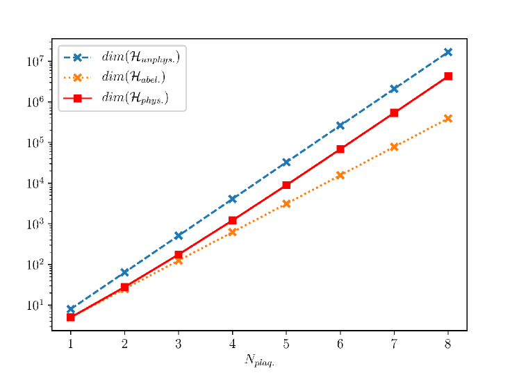
Figure 7: A plot of the data in Table III.4. As the number of plaquettes increases, the non-local physical states become dominant.

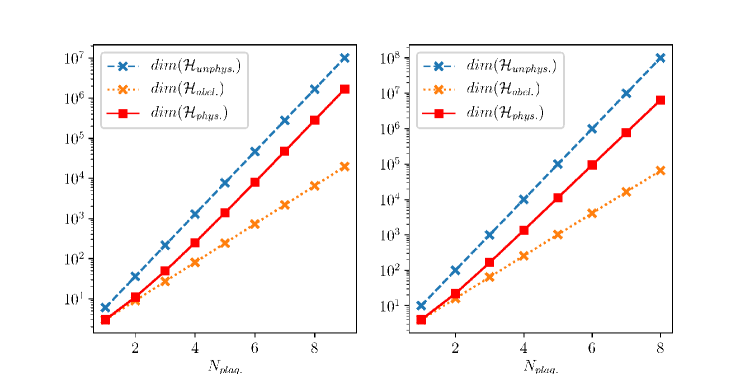
Figure 8: Scaling of the physical Hilbert space in a two-dimensional lattice gauge theory with the dihedral groups $D_{3}$ (left) and $D_{5}$ (right).

An identical scaling as with the quaternion group is obtained with the dihedral group $D_{4}$, which shares the order and number of conjugacy classes with $\mathcal{Q}_{8}$. Similar results are obtained with the dihedral groups $D_{3}$ and $D_{5}$, and the scaling of the corresponding Hilbert spaces can be seen in Fig. 8.

It can be noted that a number of solutions proposed in literature that attempt to address the geometric non-separability of the physical Hilbert space of lattice gauge theories do not address the existence of the non-local states seen here. Gauge fixing by setting links at the boundary of the entanglement region to the group identity, as suggested in Casini et al. (2014), does not change any of the arguments above if the boundary of the entanglement region is part of the maximal tree used in gauge fixing. The non-local states are not restricted to neighbouring plaquettes, and this issue is not addressed by various Hilbert space extensions schemes at the boundary Buividovich and Polikarpov (2008); Radicevic (2014). To see this, one can consider two arbitrarily space-separated gauge links, in a lattice with maximal tree gauge fixing and states in which all remaining links except the two are set to the group identity, as in Fig. 9. Then, one can consider the states in Eq. (III.4), apply the same reasoning as for the two plaquette lattice and arrive at the same conclusion: local Wilson loops cannot be used to distinguish between non-local states; one needs a Wilson loop that goes through both of the non-identity links in order to distinguish the two physical states.

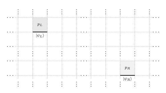
Figure 9: A geometrically inseparable state on a lattice with a non abelian gauge group. The state is such that all the links except the two labeled ones are set to the group identity.

The difficulty of expressing states on lattices with the quaternion group is also apparent when we look at electric states. The quaternion group has five representations, but only four are one-dimensional, which is insufficient to construct a local electric basis for the physical states. This does not mean that the quaternion group gauge theory, and nonabelian theories in general, do not have electric states, but only that such states are not all expressible as a tensor product of electric states on individual links. Specifically, we can always create electric states by applying Wilson loop operators on the electric vacuum $\ket{0}$, which is the electric state corresponding to the trivial representation. However, doing so with extended loops in nonabelian theories can result in inseparable states. For example, we can apply a properly normalized version of the two-plaquette loop operator using the fixed lattice in Fig. 6:

$$2U_{\vbox{\hbox{\includegraphics[height=4.52083pt]{symb/dplaq1110111}}}}^{0}\ket{0} =tr(U_{L}U_{R})\dfrac{1}{|G|}\sum_{g_{L},g_{R}\in G}\ket{g_{L}g_{R}}$$

$$=\dfrac{1}{8}\Big{(}\ket{+I}\ket{+I}+\ket{-I}\ket{-I}-\ket{+I}\ket{-I}-\ket{-I}\ket{+I}$$

$$+\sum_{a\in\{1,2,3\}}\ket{+i\sigma_{a}}\ket{-i\sigma_{a}}+\ket{-i\sigma_{a}}\ket{+i\sigma_{a}}-\ket{+i\sigma_{a}}\ket{+i\sigma_{a}}-\ket{-i\sigma_{a}}\ket{-i\sigma_{a}}\Big{)},$$ (53)

which is a state that cannot be factorized. By contrast, for a $Z_{2}$ abelian group, one would obtain:

$$U_{\vbox{\hbox{\includegraphics[height=4.52083pt]{symb/dplaq1110111}}}}^{0}\ket{0} =tr(U_{L}U_{R})\dfrac{1}{2}\Big{(}\ket{\rightarrow}\ket{\rightarrow}+\ket{\rightarrow}\ket{\leftarrow}+\ket{\leftarrow}\ket{\rightarrow}+\ket{\leftarrow}\ket{\leftarrow}\Big{)}$$

$$=\dfrac{1}{2}\Big{(}\ket{\rightarrow}\ket{\rightarrow}-\ket{\rightarrow}\ket{\leftarrow}-\ket{\leftarrow}\ket{\rightarrow}+\ket{\leftarrow}\ket{\leftarrow}\Big{)}$$

$$=\dfrac{1}{\sqrt{2}}\Big{(}\ket{\rightarrow}-\ket{\leftarrow}\Big{)}\otimes\dfrac{1}{\sqrt{2}}\Big{(}\ket{\rightarrow}-\ket{\leftarrow}\Big{)},$$ (54)

where the states $\ket{\rightarrow}$ and $\ket{\leftarrow}$ are eigenstates of $U$ with eigenvalues $+1$ and $-1$, respectively.

In principle, one could attempt to fully fix the gauge in the field basis by constraining the ancillary global gauge transformation. In order to do so, one must impose some condition on the gauge fields. Looking at the states in Eq. (III.4), the two terms in each state are related by a global gauge transformation and therefore part of the same gauge orbit. However, both states are symmetric under a $(L)\leftrightarrow(R)$ exchange, and one can conclude that a gauge fixing condition cannot be local, since a local condition, applicable equally to both factors, cannot select a single term in both states. One is left with non local conditions. Furthermore, even non local conditions that are invariant to link exchanges, such as conditions of the form $\max_{g}\sum_{x,\mu}O[gu_{x,\mu}g^{-1}]$ which maximize some functional that only has local terms, $O$, over all global gauge transformationsMandula and Ogilvie (1990) can fail to fix the gauge, since they would also fail to select a single term in either of the states in Eq. (III.4). These difficulties are reminiscent of the Gribov ambiguity from the continuum.

III.5 $SU(N)$

For continuous groups, the dimension of the local Hilbert space (physical or unphysical) is not finite. This makes the exact form of counting arguments that were used for discrete groups impossible to use. Instead, the natural extension to continuous groups is to attempt to construct a map from pairs of physical basis states on two regions of a lattice to physical basis states on the whole lattice. Or, conversely, show that such a construction is impossible because the whole lattice can support multiple physical states for a single pair of physical states on the smaller regions, when those regions are taken separately from the rest of the lattice. In other words, one can show that larger lattices support physically distinct states that are indistinguishable using local physical operators or products of local physical operators. Specifically, one can show that $\exists g_{a},g_{b}^{1},g_{b}^{2}\in SU(N)$ with

$$g_{b}^{1} \cong g_{b}^{2},$$

$$g_{a}g_{b}^{1} \ncong g_{a}g_{b}^{2},$$ (55)

where “$\cong$” denotes class equivalence. The physical meaning of that statement is that one could take the two-plaquette lattice in Fig. 6 and states

$$\ket{\psi_{1}}=\int_{G}\mathop{}\!\mathrm{d}u\ket{ug_{a}u^{-1}}_{\vbox{\hbox{\includegraphics[height=4.52083pt]{symb/dplaq1111000}}}}\ket{ug_{b}^{1}u^{-1}}_{\vbox{\hbox{\includegraphics[height=4.52083pt]{symb/dplaq0001111}}}},$$

$$\ket{\psi_{2}}=\int_{G}\mathop{}\!\mathrm{d}u\ket{ug_{a}u^{-1}}_{\vbox{\hbox{\includegraphics[height=4.52083pt]{symb/dplaq1111000}}}}\ket{ug_{b}^{2}u^{-1}}_{\vbox{\hbox{\includegraphics[height=4.52083pt]{symb/dplaq0001111}}}},$$ (56)

where we labeled the kets inside the integral as belonging to the left or right plaquette and $\mathop{}\!\mathrm{d}u$ is the Haar measure. As mentioned before, gauge invariant operators diagonal in the field basis take the form $f_{c}(U_{\mathcal{C}})$, where $\mathcal{C}$ is a closed curve of links on the lattice and $f_{c}$ is a class function. Assume $W_{\mathcal{C}}$ is such an operator with some $f_{c}$ injective over conjugacy classes. That is, $f_{c}(g_{1})=f_{c}(g_{2})$ if and only if $g_{1}\cong g_{2}$. Applying $W_{\vbox{\hbox{\includegraphics[height=4.52083pt]{symb/dplaq1111000}}}}$ and $W_{\vbox{\hbox{\includegraphics[height=4.52083pt]{symb/dplaq0001111}}}}$ to the states $\ket{\psi_{1}}$ and $\ket{\psi_{2}}$ in Eq. (III.5), we obtain:

$$W_{\vbox{\hbox{\includegraphics[height=4.52083pt]{symb/dplaq1111000}}}}\ket{\psi_{1}} =f_{c}(g_{a})\ket{\psi_{1}},$$

$$W_{\vbox{\hbox{\includegraphics[height=4.52083pt]{symb/dplaq0001111}}}}\ket{\psi_{1}} =f_{c}(g_{b}^{1})\ket{\psi_{1}},$$

$$W_{\vbox{\hbox{\includegraphics[height=4.52083pt]{symb/dplaq1111000}}}}\ket{\psi_{2}} =f_{c}(g_{a})\ket{\psi_{2}},$$

$$W_{\vbox{\hbox{\includegraphics[height=4.52083pt]{symb/dplaq0001111}}}}\ket{\psi_{2}} =f_{c}(g_{b}^{2})\ket{\psi_{2}}.$$ (57)

Since $f_{c}(g_{b}^{1})=f_{c}(g_{b}^{2})$, it follows that $W_{\vbox{\hbox{\includegraphics[height=4.52083pt]{symb/dplaq1111000}}}}\ket{\psi_{1}}=W_{\vbox{\hbox{\includegraphics[height=4.52083pt]{symb/dplaq1111000}}}}\ket{\psi_{2}},W_{\vbox{\hbox{\includegraphics[height=4.52083pt]{symb/dplaq0001111}}}}\ket{\psi_{1}}=W_{\vbox{\hbox{\includegraphics[height=4.52083pt]{symb/dplaq0001111}}}}\ket{\psi_{2}}$, and the two states are indistinguishable using the $W_{\vbox{\hbox{\includegraphics[height=4.52083pt]{symb/dplaq1111000}}},\vbox{\hbox{\includegraphics[height=4.52083pt]{symb/dplaq0001111}}}}$ operators. However, $W_{\vbox{\hbox{\includegraphics[height=4.52083pt]{symb/dplaq1110111}}}}$, the operator associated with the curve that goes around both plaquettes (without crossing), when applied to the two states above yields:

$$W_{\vbox{\hbox{\includegraphics[height=4.52083pt]{symb/dplaq1110111}}}}\ket{\psi_{1}} =f_{c}(g_{a}g_{b}^{1})\ket{\psi_{1}},$$

$$W_{\vbox{\hbox{\includegraphics[height=4.52083pt]{symb/dplaq1110111}}}}\ket{\psi_{2}} =f_{c}(g_{a}g_{b}^{2})\ket{\psi_{2}},$$ (58)

which are different by the assumption $g_{a}g_{b}^{1}\ncong g_{a}g_{b}^{2}$. The existence of group elements satisfying Eq. (III.5) can be shown explicitly for $SU(N)$:

$$g_{a}=g_{b}^{1} =\begin{pmatrix}\makebox[25.00003pt]{$e^{i\theta}$}&&&\\ &\makebox[25.00003pt]{$e^{-i\theta}$}&&\\ &&\makebox[25.00003pt]{$1$}&\\ &&&\ddots\end{pmatrix}$$

$$g_{b}^{2} =\begin{pmatrix}\makebox[25.00003pt]{$e^{-i\theta}$}&&&\\ &\makebox[25.00003pt]{$e^{i\theta}$}&&\\ &&\makebox[25.00003pt]{$1$}&\\ &&&\ddots\end{pmatrix},$$ (59)

with the dots being ones and $\theta\in(0,\pi)$. The two are conjugate since $g_{b}^{2}=hg_{b}^{1}h^{-1}$, with

$$h=\begin{pmatrix}\makebox[25.00003pt]{$0$}&\makebox[25.00003pt]{$1$}&\makebox[25.00003pt]{$$}&\\ -1&0&&\\ &&1&\\ &&&\ddots\end{pmatrix}.$$ (60)

However, $g_{a}g_{b}^{1}$ and $g_{a}g_{b}^{2}$ are clearly not conjugate, since their characters in the fundamental representation are different:

$$\operatorname{tr}(g_{a}g_{b}^{1}) =\operatorname{tr}\begin{pmatrix}\makebox[25.00003pt]{$e^{2i\theta}$}&\makebox[25.00003pt]{$$}&\makebox[25.00003pt]{$$}&\\ &e^{-2i\theta}&&\\ &&1&\\ &&&\ddots\end{pmatrix}=(N-2)+2\cos(2\theta)$$

$$\operatorname{tr}(g_{a}g_{b}^{2}) =\operatorname{tr}\begin{pmatrix}\makebox[25.00003pt]{$1$}&\makebox[25.00003pt]{$$}&\makebox[25.00003pt]{$$}&\\ &1&&\\ &&1&\\ &&&\ddots\end{pmatrix}=N.$$ (61)

Going further into a general treatment for $SU(N)$ is difficult, but one can gain more insight by restricting the discussion to $SU(2)$. Conjugacy classes in $SU(2)$ are fully described by the character of the fundamental representation. That implies that classes can be parameterized as $\operatorname{Cl}_{\theta}\stackrel{{\scriptstyle\text{def}}}{{=}}\operatorname{Cl}(\operatorname{d}(\theta))$ with $\theta\in[0,\pi]$, where we define $\operatorname{d}(\theta)=\operatorname{diag}(e^{i\theta},e^{-i\theta})$. Without loss of generality, we can pick $g_{a}=\operatorname{d}(\theta_{a}),g_{b}^{1}=\operatorname{d}(\theta_{b})$ in Eq. (III.5). We then want to see what conjugacy class $g_{a}g_{b}^{2}$ belongs to as $g_{b}^{2}$ spans $\operatorname{Cl}(g_{b}^{1})$. To do so, we pick an arbitrary $SU(2)$ element $h=\begin{pmatrix}\makebox[25.00003pt]{$\alpha$}&\makebox[25.00003pt]{$\beta$}\\ -\beta^{*}&\alpha^{*}\end{pmatrix}$, with $|\alpha|^{2}+|\beta|^{2}=1$ and calculate $\operatorname{tr}(g_{a}hg_{b}^{1}h^{\dagger})$ to obtain:

$$\operatorname{tr}(g_{a}hg_{b}^{1}h^{\dagger})=2|\alpha|^{2}\cos(\theta_{a}+\theta_{b})+2(1-|\alpha|^{2})\cos(\theta_{a}-\theta_{b}).$$ (62)

It follows that the the field basis of physical states on two plaquettes is described by three parameters: $\theta_{a},\theta_{b}\in[0,\pi]$, and $|\alpha|^{2}\equiv x\in[0,1]$. The later corresponds to distinct physical states only if $\cos(\theta_{a}+\theta_{b})\neq\cos(\theta_{a}-\theta_{b})$ which is equivalent to $\theta_{a},\theta_{b}\in(0,\pi)$. This is equivalent to the statement that a basis for physical states on a two-plaquette $SU(2)$ lattice consist of simultaneous eigenstates of Wilson loop operators $U_{\vbox{\hbox{\includegraphics[height=4.52083pt]{symb/dplaq1111000}}}},U_{\vbox{\hbox{\includegraphics[height=4.52083pt]{symb/dplaq0001111}}}},U_{\vbox{\hbox{\includegraphics[height=4.52083pt]{symb/dplaq1110111}}}}$, where $U_{\mathcal{C}}$ are like $W_{\mathcal{C}}$ above, but with $f_{c}=\operatorname{tr}$, the remaining operator, $U_{\vbox{\hbox{\includegraphics[height=4.52083pt]{symb/dplaqX}}}}$, being related Watson (1994) to the other three by the following $SU(2)$ Mandelstam constraint:

$$U_{\vbox{\hbox{\includegraphics[height=4.52083pt]{symb/dplaqX}}}}=U_{\vbox{\hbox{\includegraphics[height=4.52083pt]{symb/dplaq1111000}}}}U_{\vbox{\hbox{\includegraphics[height=4.52083pt]{symb/dplaq0001111}}}}-U_{\vbox{\hbox{\includegraphics[height=4.52083pt]{symb/dplaq1110111}}}}.$$ (63)

We can, therefore, express the physical Hilbert space on a two-plaquette $SU(2)$ lattice as

$$\mathcal{H}^{\text{phys.}}_{\vbox{\hbox{\includegraphics[height=4.52083pt]{symb/dplaq1110111}}}}=(P\otimes P)\oplus(P\otimes B)\oplus(B\otimes P)\oplus(B\otimes B\otimes X),$$ (64)

where $P=\operatorname{span}\big{\{}\ket{\operatorname{d}(0)},\ket{\operatorname{d}(\pi)}\big{\}}$, $B=\operatorname{span}\big{\{}\ket{\operatorname{Cl}_{\theta}}|\;\theta\in(0,\pi)\big{\}}$, and $X=\operatorname{span}\big{\{}\ket{x}|\;x\in[0,1]\big{\}}$. This shows a similar structure to the physical space of the two plaquette lattice with a Quaternion group, but where $X$ enters as a factor in a term rather than being a term in a direct sum. For simplicity, in the discussion that follows, we will focus only on the last term of Eq. (64). It is, in principle, possible to write $X$ as a product of two factors in the sense that one may be able to find $\mathcal{H}^{\text{phys.}}_{1}$ and $\mathcal{H}^{\text{phys.}}_{2}$ such that there is a one-to-one mapping $(\theta_{a},\theta_{b},x)\overset{f}{\longleftrightarrow}(u_{1},u_{2})$, with field basis vectors $\ket{u_{1}}\in\mathcal{H}^{\text{phys.}}_{1},\ket{u_{2}}\in\mathcal{H}^{\text{phys.}}_{2}$ and with $u_{1},u_{2}$ taking values in some connected subspace of $\mathbb{R}$ such that $u_{i}$ have the appearance of fields. However, this cannot be done while preserving certain properties of the mapping. For example, if we wanted to analytically relate the algebras of $\mathcal{H}^{\text{phys.}}_{i}$ with the algebra of $\mathcal{H}^{\text{phys.}}_{\vbox{\hbox{\includegraphics[height=4.52083pt]{symb/dplaq1110111}}}}$, $f$ would need to be analytic and thus continuous. That is, we would need to find a bijective and continuous function from a connected subspace $A=\{(\theta_{a},\theta_{b},x)\}\subset\mathbb{R}^{3}$ to a connected subspace $B=\{(u_{1},u_{2})\}\subset\mathbb{R}^{2}$, which is impossible, as can be seen from the following argument: Consider a closed curve $\mathcal{C}\subset B$. Then $B\setminus\mathcal{C}$ is disconnected. By continuity of $f$, the pre-image $A\setminus\mathcal{S}=f^{-1}(B\setminus\mathcal{C})$, where $\mathcal{S}=f^{-1}(\mathcal{C})$, should also be disconnected, which implies that $\mathcal{S}$ is a surface in $A$. The surface $\mathcal{S}$ is connected since $\mathcal{C}$ is connected by construction. Let $x_{1},x_{2}\in\mathcal{S}$ be two distinct points. The set $\mathcal{S}^{\prime}=\mathcal{S}\setminus\{x_{1},x_{2}\}$ remains connected. However, the image of $\mathcal{S}^{\prime}$ is now $\mathcal{C}^{\prime}=\mathcal{C}\setminus\{f(x_{1}),f(x_{2})\}$ and the points $f(x_{1})$ and $f(x_{2})$ divide $\mathcal{C}$ into two disconnected curve segments. Thus, we arrive at a contradiction, since $\mathcal{S}^{\prime}$ is connected, but its image $\mathcal{C}^{\prime}$ through a continuous function is not.

We can also prove a less general but possibly more illuminating statement: there is no way to construct the function $f$ such that it does not mix the subspaces of $\theta_{a}$ and $\theta_{b}$. That is, if $(u,v)=f(\theta_{a},\theta_{b},x)$ and $f$ is bijective, there is no bijective $g$ such that

$$u =g(\theta_{a},x)$$

$$v =g(\theta_{b},x).$$ (65)

To see this, take $x_{1}\neq x_{2}$ such that $(u_{1},v_{1})=f(\theta_{a},\theta_{b},x_{1})$ and $(u_{2},v_{2})=f(\theta_{a},\theta_{b},x_{2})$. Then $u_{1}=g(\theta_{a},x_{1}),v_{2}=g(\theta_{b},x_{2})$. Since $(u_{1},v_{1}),(u_{2},v_{2})\in\mathcal{H}^{\text{phys.}}_{1}\otimes\mathcal{H}^{\text{phys.}}_{2}$ then also $(u_{1},v_{2})\in\mathcal{H}^{\text{phys.}}_{1}\otimes\mathcal{H}^{\text{phys.}}_{2}$. This implies that $\exists(\theta_{a}^{\prime},\theta_{b}^{\prime},x^{\prime})$ such that $(u_{1},v_{2})=f(\theta_{a}^{\prime},\theta_{b}^{\prime},x^{\prime})$. But that implies that $g(\theta_{a},x_{1})=g(\theta_{a}^{\prime},x^{\prime})$, which, by the bijective condition of $g$ implies that $\theta_{a}=\theta_{a}^{\prime},x_{1}=x^{\prime}$. Similarly, we obtain that $\theta_{b}=\theta_{b}^{\prime},x_{2}=x^{\prime}$ and thus $x_{1}=x_{2}$, which is a contradiction.

While the existence of the condition in Eq. (III.5) exists for higher $SU(N)$, the one-to-one mapping between the character in the fundamental representation and the conjugacy class does not necessarily hold. For example, in $SU(4)$, $\operatorname{diag}(1,-1,1,-1)$ and $\operatorname{diag}(i,-i,i,-i)$ have the same trace, but are not in the same conjugacy class. The resulting complexity is beyond the scope of this paper.

IV The role of matter fields

We now turn to theories where both matter and gauge fields are present. In contrast with pure gauge theories, the addition of matter fields results in the ability to factor the Hilbert space locally. For a somewhat related discussion, please see Harlow (2015).

We use a similar strategy as with pure gauge lattices: fix the gauge in order to understand how the physical space looks like, then construct, from the unphysical algebra, gauge invariant operators that generate gauge invariant states which span a space isomorphic to the gauge fixed space. The arguments presented here hold in a general sense, being applicable to general groups and sets they act on. However, for simplicity, we restrict the discussion to matter fields that take the form of vectors.

We assume a matter field that transforms in the familiar way (Eq. (31)) under gauge transformations, which we repeat here:

$$\ket{\phi(x)} \rightarrow\ket{\phi^{\prime}(x)}=\ket{g(x)\phi(x)}.$$ (66)

We fix the gauge as before, by setting links to the group identity on a maximal tree. As before, we are left with a global gauge transformation, which leaves the identity links unchanged. However, matter fields at vertices attached to those links are not invariant under the global gauge transformation, and we cannot simply discard all but the unfixed links from the gauge-fixed space. We are left with d.o.f. corresponding to the unfixed links as well as those corresponding to matter fields at the vertices. The global gauge transformation now amounts to an overall phase of the matter fields. We can fix the global gauge by rotating everything such that the field on one chosen vertex $x_{0}$ points in a gauge direction of our choice. Specifically, field basis vectors for the matter fields can be written as

$$\ket{\phi(x)} =\ket{v(x)1_{\phi}\tilde{\phi}(x)},$$ (67)

with $v(x)$ being gauge group $G$ valued, $1_{\phi}$ being a representative vector that elements in $G$ act on faithfully, and $\tilde{\phi}(x)$ being a scalar. We assume, for simplicity, that the space of the kets in the RHS of Eq. (67) can be factored as $\ket{v(x)1_{\phi}\tilde{\phi}(x)}=\ket{v(x)}\otimes\ket{\tilde{\phi}(x)}$. We fix the gauge fully by picking a $x_{0}$ and using a global gauge transformation

$$\ket{v(x)}\otimes\ket{\tilde{\phi}(x)}\rightarrow\ket{v(x_{0})^{-1}v(x)}\otimes\ket{\tilde{\phi}(x)},$$ (68)

which implies

$$\ket{v(x_{0})}\otimes\ket{\tilde{\phi}(x_{0})}\rightarrow\ket{I_{G}}\otimes\ket{\tilde{\phi}(x_{0})},$$ (69)

where $I_{G}$ is the gauge group identity. We now have $N_{V}-1$ group-valued d.o.f., where $N_{V}$ is the number of vertices in the lattice, corresponding to the gauge portion of the matter fields at all vertices except for $x_{0}$. From graph theory, we know that a maximal tree always has $N_{V}-1$ edges, which implies that we are also left with $N_{L}-(N_{V}-1)$ unfixed link d.o.f.. The total number of gauge-valued d.o.f. is then

$$N_{G}=N_{V}-1+N_{L}-(N_{V}-1)=N_{L}.$$ (70)

That is, after full gauge fixing, we have precisely as many gauge-valued d.o.f. as we have links in the lattice and as many scalar valued d.o.f. as we have vertices. We can, therefore, construct a physical Hilbert space from the unphysical one by a re-definition of variables:

$$\phi^{\prime}(x) =\tilde{\phi}(x)$$

$$u_{i}^{\prime}(x) =v(x)^{-1}u_{i}(x)v(x+\hat{i}),$$ (71)

where $x+\hat{i}$ denotes a neighbouring vertex in the $i$ direction from $x$. Both the redefined variables are now gauge invariant quantities. The primed matter field is invariant by construction. For $u^{\prime}$, we note that the unphysical field $v$ transforms as $v(x)\rightarrow g(x)v(x)$. Then, using Eq. (32)

$$\ket{u_{i}^{\prime}(x)} \rightarrow\ket{v(x)^{-1}g(x)^{-1}g(x)u_{i}(x)g^{-1}(x+\hat{i})g(x+\hat{i})v(x+\hat{i})}$$

$$=\ket{v(x)^{-1}u_{i}(x)v(x+\hat{i})}$$

$$=\ket{u_{i}^{\prime}(x)}.$$ (72)

The physical interpretation of the fields $u^{\prime}$ is that, in the corresponding electric basis, electric fluxes are now automatically associated with the local charges that create them. These charges are not coupled to local energy eigenstates of the primed matter sector, except possibly through dynamics. The physical Hilbert space of the theory is then:

$$\mathcal{H}^{\text{phys.}}=\bigotimes_{x}\mathcal{H}_{\phi^{\prime}}\otimes\bigotimes_{x,i}\mathcal{H}_{u^{\prime}}.$$ (73)

That is, the local fields $\phi^{\prime}(x)$ and $u^{\prime}_{i}(x)$ form a complete set of gauge invariant d.o.f. for the theory. It is important here that the matter field transform in the fundamental representation of the gauge group or a super-representation of it. If the matter field carries only a sub-representation of the gauge group, we can at most reduce the theory to a theory gauged with a subgroup $G^{\prime}$ of $G$. This may still prove useful if $G^{\prime}$ is abelian.

In terms of the the physical Hilbert space, it is important to note here that the space of a gauge-matter theory on a lattice is locally factorizable and exhibits none of the issues seen in pure gauge theories, abelian or otherwise. In fact, for the purpose of factorizing the Hilbert space of a theory into bipartite geometrical factors, a single matter field on the boundary between regions suffices Watson (1994). To illustrate this, we note that the local factorization in Eq. (73) relies on the existence of entities that transform like standard matter fields, as in Eq. (66). Such entities can be constructed from a matter field at a single point in space, $x_{0}$, and a Wilson line that connects $x_{0}$ with some other point, where Wilson lines are like Wilson loops (see Eq. (35)) except on an open curve:

$$V_{\mathcal{C}}(x) =V(x_{0})U_{\mathcal{C}}(x_{0},x)$$

$$=V(x_{0})U_{i_{0}}(x_{0})U_{i_{1}}(x_{1})\cdots U_{i_{n}}(x_{n})$$ (74)

where $x_{k}+\hat{i}_{k}=x_{k+1}$ are points along the open curve $\mathcal{C}$ starting at $x_{0}$ and ending at $x$. One can then check that $V_{\mathcal{C}}(x)$ transforms the same as as $V(x)$ under a gauge transformation. This allows one to construct a physical space in a manner similar to that used to obtain the space in Eq. (73). This, like any solution that adds d.o.f. on a fictive boundary, is likely flawed. Specifically, such a solution would make it difficult to formulate a well defined area law for entanglement entropy. An area law is a dependence between the entanglement entropy of a specific state on the Hilbert space of a theory (typically the vacuum state) and the area of the boundary separating the two regions for which the entanglement entropy is calculated. To make such a law universal would imply that boundaries entering the calculation are entirely arbitrary. If d.o.f. were defined only on boundaries, of which there were many, we would also have have multiple distinct Hilbert spaces, the choice of which would depend on precisely what regions we use in calculating the entanglement entropy. This would lead to an ill defined theory and an equally ill defined vacuum state.

V Conclusions

We have shown that in some cases that could be reasonable analyzed, the physical Hilbert space of pure non-abelian lattice gauge theories does not admit a geometric factorization. We did so using simple counting arguments, since many other approaches can be complex and can drift towards fundamental issues in quantum mechanics and field theory that are not entirely settled.

We have also shown that the addition of matter fields changes the problem in a fundamental way: it makes a factorization both straightforward and universal across gauge groups. It leads to a well defined and complete set of physical d.o.f. on Hamiltonian lattice gauge theories. It is perhaps fitting that reality appears to favor theories with matter.

The discussion here is somewhat narrow. We assume that the Hilbert space of matter fields is some space of square integrable functions. While this has to be true, for the simple reason that it induces a norm, which is needed for a sensible quantum theory, the precise Hilbert space will also depend on the potential in the Hamiltonian. Furthermore, when also involving interactions with a gauge field, the problem becomes more complex due to the interaction terms. The amount of information that can be gained from an analysis that does not involve dynamics for such cases is necessarily limited.