Space-time deterministic graph rewriting

Abstract

We study non-terminating graph rewriting models, whose local rules are applied non-deterministically—and yet enjoy a strong form of determinism, namely space-time determinism. Of course in the case of terminating computation it is well-known that the mess introduced by asynchronous rule applications may not matter to the end result, as confluence conspires to produce a unique normal form. In the context of non-terminating computation however, confluence is a very weak property, and (almost) synchronous rule applications is always preferred e.g. when it comes to simulating dynamical systems. Here we provide sufficient conditions so that asynchronous local rule applications conspire to produce well-determined events in the space-time unfolding of the graph, regardless of their application orders. Our first example is an asynchronous simulation of a dynamical system. Our second example features time dilation, in the spirit of general relativity.

1 Introduction

In short Distributed models of physical, biological, social or technological objects are often composed of interacting elements (particles, cells, agents, processes etc.) that evolve according to local rules. From this local evolution, the global evolution may be defined in various ways. Dynamical systems like cellular automata assume a global clock, each element synchronously undergoing one local rule step at each tick. Rewrite systems on the other hand assume that each element asynchronously performs a local rule step, whilst the other may remain unchanged. Synchronism is often criticised for being costly and physically unrealistic, but asynchronism leads to an inherent lack of determinism and inconsistencies therein. The paper shows that, even for asynchronous graph rewriting, a strong form of determinism, namely space-time determinism, is still possible. For this purpose it introduces a formalism for graph rewriting based on a DAG of dependencies and some local rule. It proves one proposition and one theorem, whereby local conditions on the local rule entail that its asynchronous applications produce well-determined events.

Dynamical systems refer to the global evolution of an entire configuration at time $t$ into another at time $t+1$, $t+2$ etc., iteratively. Whether the dynamical system is a grid-based model (e.g. representing particles [1, 2], fluids [3, 4], traffic jams [5], demographics and regional development or consumption [6, 7]) or a more flexible graph-based model (e.g. representing physical systems [8], computer processes [9], biochemical agents [10], economical agents [11], users of social networks, etc.), there are just countless many reasons why we may want to simulate them on a computer—after all this is the daily bread of many. Usually the computer simulation of dynamical systems, whether through numerical schemes, cellular automata or parallel graph rewriting, works by implementing the global evolution as the synchronous (or almost synchronous [12]) application of a local rule, i.e. repeatedly and simultaneously across space.

Synchronism is often criticised however, on the basis that: 1/ It is a costly resource, which prevents parallelism unless we are willing to pay the price of expensive clock synchronization mechanisms. 2/ It is often dubbed as physically unrealistic. One hears sentences like : “How can you expect that nature applies the same rule everywhere at once?”. This is a fair point as relativistic physics clearly departs from the idea of a global time across the universe. In particular the ‘time covariance’ symmetry entails that it is perfectly legitimate to evolve just a small region of space, whilst keeping the rest of it virtually unchanged.

Asynchronism fits this picture better. It consists in the application of the local rule at totally arbritrary places. Theoretical Computer Science draws a clear distinction between deterministic; probabilistic; and non-deterministic evolutions—asynchronous evaluation strategies belong to the later. Non-deterministic evolutions are studied for a variety of reasons in Computer Science (e.g. complexity theory, safety analysis…): one of them is precisely that it is often more compelling to just leave the transition system under-determined. This is typically the case in Rewriting theory, for instance when the rewrite rules arise as a computationally-oriented version of an equality, e.g. $1+1\to 2$. Then, term $1+1+1$ may evolve into $2+1$, but it may also evolve into $1+2$, non-deterministically. This feels right, because: 1/ an underlying symmetry tells us there is no reason to favour one over the other and 2/ ultimately, if what matters is the end result, we are reassured by the fact that $2+1\to 3$ and $1+2\to 3$. Non-determinism, therefore, is not incompatible with subtler notions of determinism. Developing such notions is a matter in its own right, let us take a deep breath and dive in there.

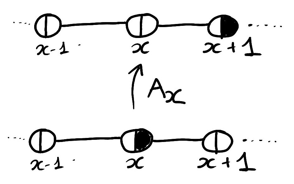
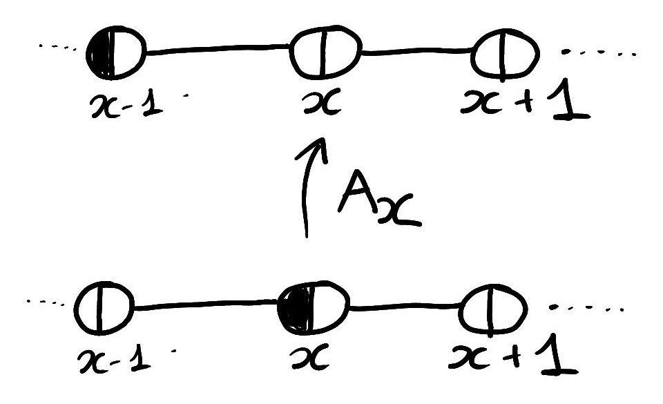
(a) $G$.

(b) $A_{345671}G$.

(c) $A_{543217}G$.

(d) $A_{65432}A_{345671}G=A_{23456}A_{345671}G$.

Figure 1: Confluence yet inconsistencies. The local rule transports right-moving particles to the right and left-moving particles to the left, without interactions. $(a)$ We start with a left-moving particle in $7$ and a right-moving particle in $1$. $(b)\&(c)$ The point of collision between the two particles is not well defined, it depends on the evaluation strategy. Here $A_{71}G$ is short for $A_{7}(A_{1}G)$. $(d)$. Still, the system is confluent, as the divergent configurations can be both evolve into the last.

Confluence ensures that the non-determinism introduced by the order of application of the rewrite rules, will not matter to the end result, yielding a well-determined, unique normal form e.g. $3$ in the above example. More generally the confluence of a set of rewrite rules states that if the evolutions $a\to^{*}b$ and $a\to^{*}c$ are possible, then the evolutions $b\to^{*}d$ and $c\to^{*}d$ also are. The promise made is that: “If the computational process reaches a result, this result will be the same as that following any another conclusive computational route”. E.g. contributions [13, 14, 15, 16, 17] deal with the case when the computational process eventually produces a graph a result, through successive rewrites.
But, what if our computational process generates not just in one result, but a succession of them…is confluence bearing any promise, then? Unfortunately, it hardly provides any guarantee, e.g. rewrite rules yielding every possible result are trivially confluent. Things get even worse if we are interested in modelling not just one computational process, but an entire network of interacting processes, each of them generating one result after the other, possibly passing them on to their neighbours…i.e. distributed computation, possibly non-terminating, including dynamical systems, e.g. particle systems. For instance, Fig. 1 shows left and right-moving particles on a line, where left versus right is indicated by the ports along the edges. The local rule simply has them move, a little thought show that the system is confluent. Yet, depending upon the chosen order of applications, one finds that one particle propagates much faster than the other, yielding the collision to occur at very different places. Whilst this example is designed to emphasize these issues, it is clear that, when it comes to dynamical systems, asynchronous evaluation strategies may lead to inconsistent results, nonphysical effects (e.g. superluminal signalling), and pathological dynamical behaviours (e.g. over boolean networks [18, 19] and cellular automata [20, 21]). This is a major deterrent to their usage, and the notion of confluence is no fix to that. To fix this, we need a stronger such “subtle notion of determinism”, here are two.

Weak consistency is the promise each of our interacting processes will systematically obtain the same succession of results, independent of the concrete order of asynchronous application of the local rule. I.e. this is a local version of unique normal form property, repeated across space-time. We obtain a weak consistency proposition, stating that if local rule applications commute, then the normal form of each space-time event $t.x$ is, if reached, well-determined in terms of its internal state and connectivity. In our formalism, the normal form of an event is a minimal vertex of the DAG, as it no longer awaits for a previous result in order to get computed.

Full consistency, a.k.a. space-time determinism, is the even stronger property that all events in space-time be well-determined. For our interacting processes, this is the promise that each of them will systematically obtain the same provisional results, provisional upon the information that is yet to be retrieved from the neighbouring processes. I.e. “same progress, same result”. For simulating dynamical systems this is the relevant notion, as illustrated by Fig. 5 & 6 and discussed at length when we present this example, which fixes the issues with the asynchronous computer simulation left and right-moving particles. Notice how in this example the internal state associated to a space-time event $t.x$ depends upon its set incoming ports. This is in line with Physics, where the state of a field at a space-time point does depend on the way space-time is foliated at this point, i.e. on the angle of the space-like cut. We obtain a full consistency theorem, stating that if local rule applications commute and strictly decrease the privately accessible incoming ports of all modified vertices (Fig. 10), then the internal state and connectivity of each vertex is fully determined by its incoming ports (Fig. 9).

Dynamical geometry. We do not restrict ourselves to work over a fixed lattice or a fixed boolean network, here. Our processes starts with some given neighbours, but they can then connect with the neighbours or their neighbours, as well as disconnect. The DAG of dependencies is both a constraint upon the evolution, and a subject of the evolution, allowing us to express intriguing effects such as time dilation, reminiscent of general relativity, see Fig. 8.

Applications. Whilst mainly of theoretical nature, we hope to have convinced the reader that this work may contribute to the efficient parallel schemes for the implementation of dynamical system and distributed systems—doing away with any expensive clock synchronisation mechanisms and replacing it with a cheap DAG. This was not our original motivation: the applications we pursue lie at the crossroad with Physics, as we seek for a mathematically sound, constructive framework for discrete models of general relativity [22]. From a general philosophy of science point of view, we find it compelling to reconcile asynchronism and determinism.

Plan of the paper. Sec. 2 makes specific the kind of DAG we use, the way we name each vertex, the fact that edges are between ports of vertices, and what is meant by a local rule. Sec. 3 provides an example of how to perform the asynchronous simulation of a dynamical system, at the cost of introducing “metric” information in the form of these DAG so as to capture the relative advancement of the computation in a region with respect to another. Sec. 4 shows how, having introduced this DAG, one can manipulate it to achieve time dilation effects. An analogy is drawn with general relativity, where the concepts of time covariance, metric, background-independence and dynamical geometry, lead to time dilation. Sec. 5 introduces weak and full consistency as well as the corresponding theorems, constituting our main technical contributions. Sec. 6 summarizes the results, compares them to the related works, and provides some perspectives.

2 Graphs and local rules

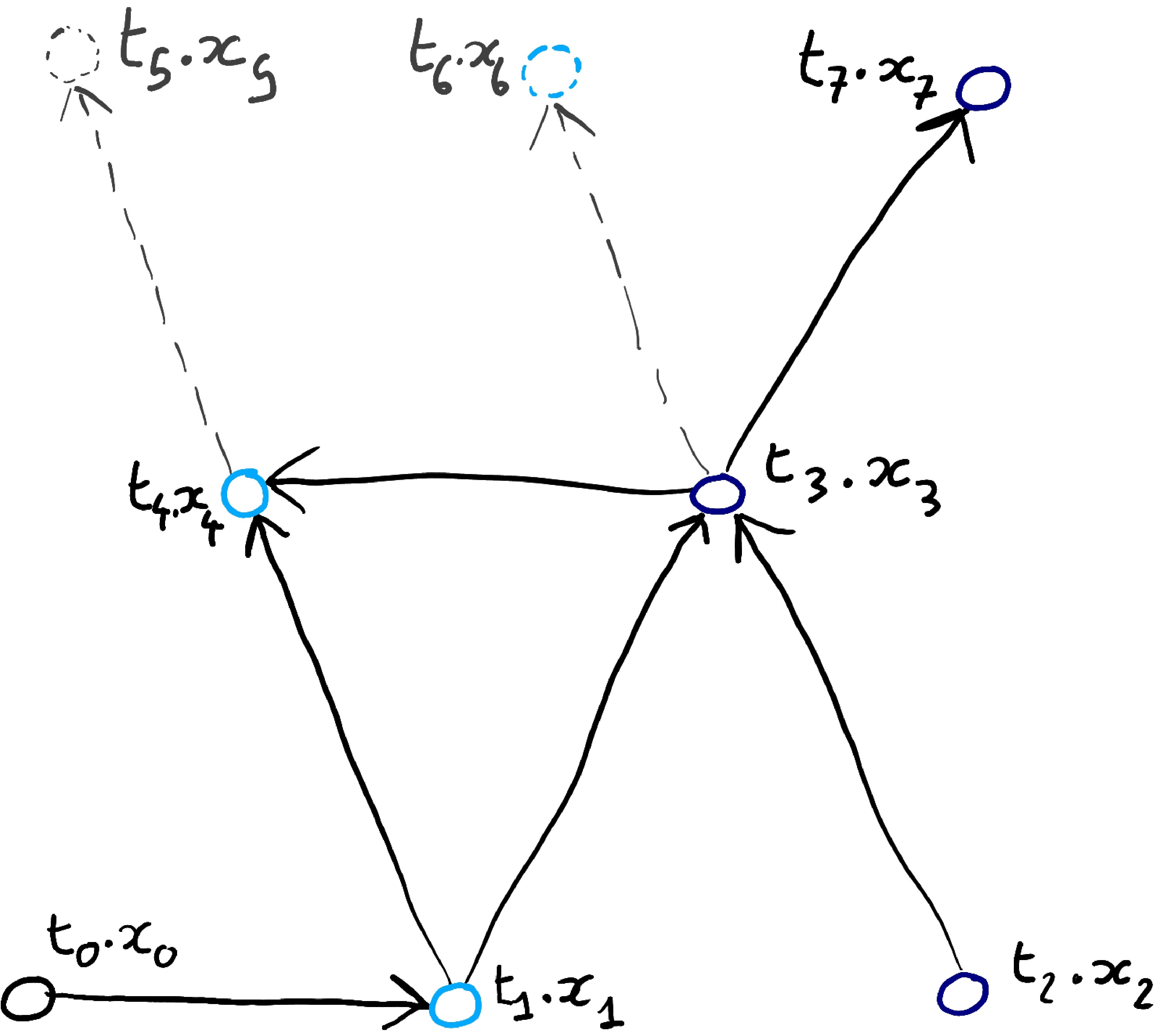
(a) $G$

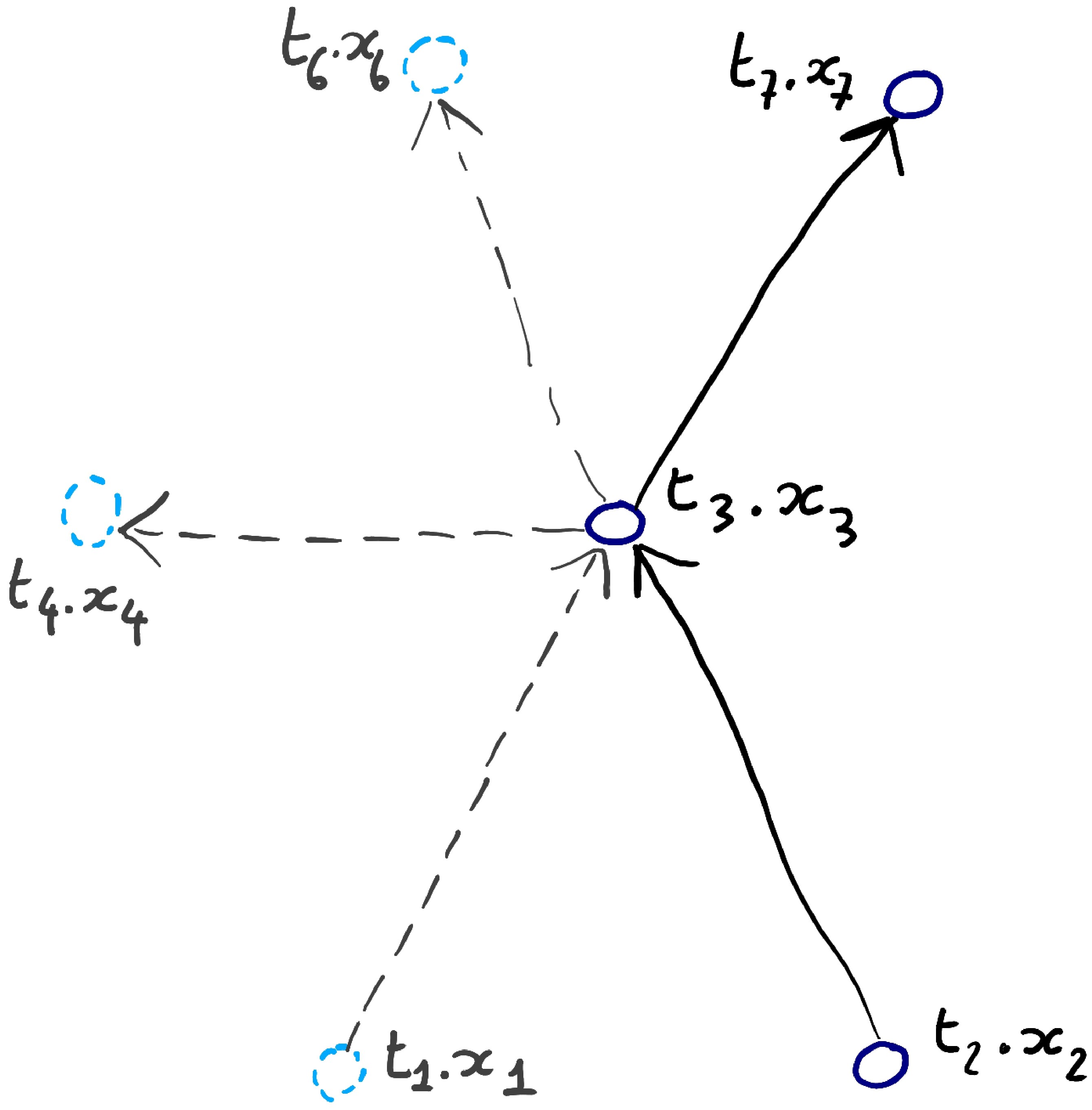
(b) $G_{X^{-}}$

Figure 2: Border of graph, border of set. We consider a graph $G$ and a set of positions $X=X^{-}\cup B_{X}=\{x_{i}\mid x_{i}\notin\{x_{5},x_{0}\}\}$ corresponding to the internal ($X^{-}$ in dark blue–e.g. $t_{3}.x_{3}$) and border vertices ($B_{X}$ in cyan) of an induced subgraph $G_{X^{-}}$. Entire graphs have borders, as shown pointed by the dashed lines for $(a)$ $G$ and $(b)$ $G_{X^{-}}$. But we also say that the set $X$ has border $B_{X}$ in $G$ if $X^{-}$ is the largest subset $X^{\prime}\subseteq X\cap X(\mathrm{I}_{G})$ such that $\mathrm{V}_{G_{X^{\prime}}}\subseteq{\scriptstyle\mathbb{Z}}.X$. This is the case in $(a)$ and $(b)$.

We start by formally introducing the type of graph that we consider: coloured directed acyclic port graphs. Vertex names $t.x$ are made of a time tag $t$ and a position $x$.

Definition 1 (Positions, ports, states, names)

Let ${\mathcal{X}}$ be an infinite countable set of positions. Let $\pi$ be a finite set of ports and $\Sigma$ be a finite set of states. Let us denote ${\mathcal{V}}:=\{\,t.x\mid(t,x)\in\mathbb{Z}\times{\mathcal{X}}\,\}$ and call its elements names.

For any subset $U\subseteq{\mathcal{V}}$, let us define $(U\!:\!\pi):=\{\,(u\!:\!a)\mid u\in U,\,a\in\pi\,\}$. Let us also denote $\overline{U}:=\mathcal{V}\setminus U$, and ${\scriptstyle\mathbb{Z}}.U:=\{\,t.x\mid t\in\mathbb{Z},x\in X(U)\,\}$. Given any $u=t.x\in\mathcal{V}$, let us denote $t^{\prime}.u$ for $(t^{\prime}+t).x\in{\mathcal{V}}$.

Definition 2 (Graphs)

A graph $G$ is given by a tuple $(\mathrm{I}_{G},\mathrm{B}_{G},\mathrm{E}_{G},\sigma_{G})$ where:

• $\mathrm{I}_{G}\subseteq{\mathcal{V}}$ has its elements called internal vertices of $G$,

• $\mathrm{B}_{G}\subseteq{\mathcal{V}}$ has its elements called border vertices of $G$,

• $\mathrm{E}_{G}\subseteq((\mathrm{I}_{G}\cup\mathrm{B}_{G})\!:\!\pi)^{2}\setminus(\mathrm{B}_{G}\!:\!\pi)^{2}$ has its elements called (oriented) edges, and

• $\sigma_{G}:\mathrm{I}_{G}\rightarrow\Sigma$ maps each internal vertex to its states.

We denote $\mathrm{V}_{G}:=\mathrm{I}_{G}\cup\mathrm{B}_{G}$. This tuple has to be such that:

• Vertex partitioning: $\mathrm{I}_{G}\cap\mathrm{B}_{G}=\emptyset$,

• Unicity of positions: $\forall t.x,t^{\prime}.x^{\prime}\in{\mathrm{V}_{G}},\,x=x^{\prime}\Rightarrow t=t^{\prime}$,

• Port non-saturation. $\forall(u\!:\!a,v\!:\!b),(u^{\prime}\!:\!a^{\prime},v^{\prime}\!:\!b^{\prime})\in{\mathrm{E}_{G}},\,u\!:\!a\neq v^{\prime}\!:\!b^{\prime}\,\wedge\,u\!:\!a=u^{\prime}\!:\!a^{\prime}\Leftrightarrow v\!:\!b=v^{\prime}\!:\!b^{\prime}$, and

• Border attachment: $\forall u\in\mathrm{B}_{G},\,\exists(v\!:\!a,v^{\prime}\!:\!a^{\prime})\in\mathrm{E}_{G}\text{ such that }u\in\{\,v,v^{\prime}\,\}$, and

• Acyclicity: the set of edges does not induce any cycle.

We denote by $\mathcal{G}$ the set of all graphs. Given $G\in\mathcal{G}$, we call $\mathrm{Past}(G)\subseteq\mathrm{V}_{G}$ the minimal vertices of $G$.

Summarizing, each position $x$ only appears once, each vertex port $:\!a$ can only be used once, and border vertices are only there to express dangling edges from (or to) internal vertices. Next, the subgraph induced by vertices $U$ is the smallest graph containing $U$ and the edges attached to $U$ (see Fig. 2):

Definition 3 ((Induced) subgraph and borders.)

We write $H\subseteq G$ and say that $H$ is a subgraph of $G$ whenever:

$$\mathrm{V}_{H}\subseteq\mathrm{V}_{G}\,\wedge\,\mathrm{I}_{H}\subseteq\mathrm{I}_{G}\,\wedge\,\mathrm{E}_{H}\subseteq\mathrm{E}_{G}\,\wedge\,\sigma_{H}=\sigma_{G}\mathrel{\!\raisebox{-2.15277pt}{$|$}}_{\mathrm{I}_{H}},$$

where $\sigma_{G}\mathrel{\!\raisebox{-2.15277pt}{$|$}}_{\mathrm{I}_{H}}$ denotes the function $\sigma_{G}$ restricted to the domain $I_{H}$. This relation is a partial order on ${\mathcal{G}}$. We denote by $G\cup G^{\prime}$ and $G\cap G^{\prime}$ the join and meet of $G$ and $G^{\prime}$ in the $\subseteq$-order when they exist.

We write $H\sqsubseteq G$ and say that $H$ is an induced subgraph of $G$ whenever $H\subseteq G$ and $H$ is the biggest subgraph of $G$ having this set of internal vertices, i.e. $\forall H^{\prime}\in{\mathcal{G}},H^{\prime}\subseteq G\wedge\mathrm{I}_{H^{\prime}}=\mathrm{I}_{H}\implies H^{\prime}\subseteq H$. This is also a partial order on ${\mathcal{G}}$ and we denote by $G\sqcup G^{\prime}$ and $G\sqcap G^{\prime}$ the join and meet of $G$ and $G^{\prime}$ in the $\sqsubseteq$-order when they exist.

Given a subset $U\subseteq\mathcal{V}$, we write $G_{U}$ for the induced subgraph of $G$ such that $\mathrm{I}_{G_{U}}=U\cap\mathrm{I}_{G}$. We also write $G_{u}$ for $G_{\{u\}}$. For a subset $X\subseteq\mathcal{X}$, we write $G_{X}$ for the induced subgraph $G_{{\scriptstyle\mathbb{Z}}.X}$. We write $X^{-}(G)$ or just $X^{-}$ the set $\{x\in X\,|\,x\in X(\mathrm{I}_{G})\wedge\mathrm{V}_{G_{x}}\subseteq{\scriptstyle\mathbb{Z}}.X\}$, and call these the internal vertices of $X$ in $G$. We write $\mathrm{B}_{X}(G)$ or just $\mathrm{B}_{X}$ the set $B_{G_{X^{-}}}$, and call these the border vertices of $X$ in $G$, see Fig.2.

Notice how $G=G_{X}\sqcup G_{\overline{X}}$. This decomposition will allow us to define the action of our local rules. We will proceed as follow. First we define operators $A_{(-)}$ which, given a position $x$ rewrite the graph $G$ as $A_{x}G$. Second we define a neighbourhood scheme ${\mathcal{N}}$ which, given a position $x$, selects a subset of nearby positions $\mathcal{N}_{x}(G)$. Third we say that $A_{(-)}$ is ${\mathcal{N}}$-local if the action of $A_{x}$ is to replace just the left hand side of $G=G_{\mathcal{N}_{x}(G)}\sqcup G_{\overline{\mathcal{N}_{x}(G)}}$, independently of the right hand side—an operation which can likely be formalised as a double push-out [23].

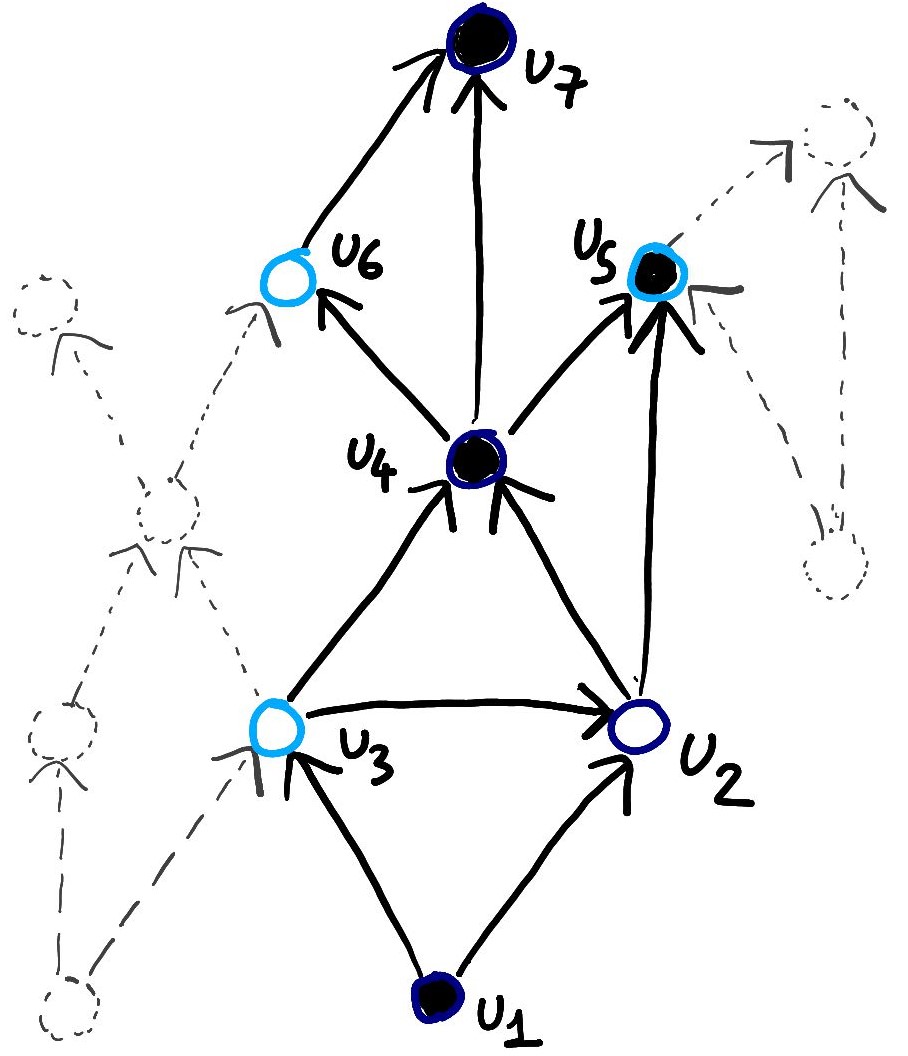
(a) $G$

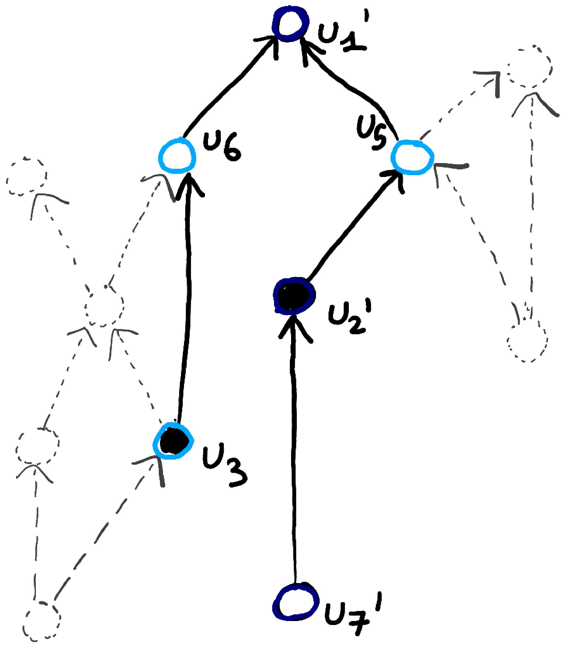
(b) $A_{x_{1}}G$

Figure 3: Action of a local rule $A_{(-)}$ centered on a vertex $u_{1}=t_{1}.x_{1}$. It affects the vertices of ${\scriptstyle\mathbb{Z}}.\mathcal{N}_{x}(G)$ that are circled dark blue & cyan. Dark blue vertices (e.g. $u_{1},u_{4}$) can be almost arbitrarily modified whereas cyan vertices must have their names and external edges preserved. Internal states $\Sigma=\{0,1\}$ are represented by white and black.

Definition 4 (Neighbourhood scheme)

A neighbourhood scheme ${\mathcal{N}}$ is an operator from $\mathcal{P}(\mathcal{X})\times{\mathcal{G}}$ to $\mathcal{P}(\mathcal{X})$ mapping a pair $(\omega,G)$ to $\mathcal{N}_{\omega}(G)\subseteq\mathcal{X}$ such that:

• Reachability: $\forall x\in\mathcal{N}_{\omega}(G),\,\exists p:\omega\rightarrow x$.

where $p:\omega\rightarrow x$ denotes a directed path in $\mathrm{E}_{G}$ from some element of $\omega$ to $x$.
The input $\omega$ is formally a set of vertices, however we will often apply ${\mathcal{N}}$ to $\omega\in\mathcal{X}^{*}$ implicitly referring to the underlying set. When $G$ is clear from context, we write ${\mathcal{N}_{\omega}}$ instead of $\mathcal{N}_{\omega}(G)$.

Note that ${\mathcal{N}^{-}_{\omega}}$ refers to the internal vertices of ${\mathcal{N}_{\omega}}$ with respect to $G$ as in Def. 2. Notice also that our definition of a neighbourhood schemes is quite abstract and permissive, possibly allowing for global criteria to decide whether a closeby vertex should be encompassed within the neighbourhood or not. To forbid this to happen we define extensivity. It asks that the neighbourhood $\mathcal{N}_{\omega}(G)$ as computed by the function ${\mathcal{N}}$ over a graph $G$, be the same as that computed over a big enough subgraph of $G$. This can be understood as a form of graph-locality of the neighbourhood scheme $\mathcal{N}()$ itself, for instance if $\mathcal{N}_{\omega}(G)$ is computed step by step starting from $\omega$ until it hits a ‘wall’ i.e. a local ending criterion, then it will be extensive.

Definition 5 (Extensivity)

$G_{\mathcal{N}_{\omega}}\sqsubseteq H\sqsubseteq G$ implies $\mathcal{N}_{\omega}(G)=\mathcal{N}_{\omega}(H)$.

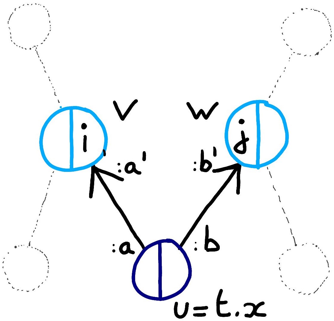
(a) $G_{{\mathcal{N}_{x_{1}}}}$.

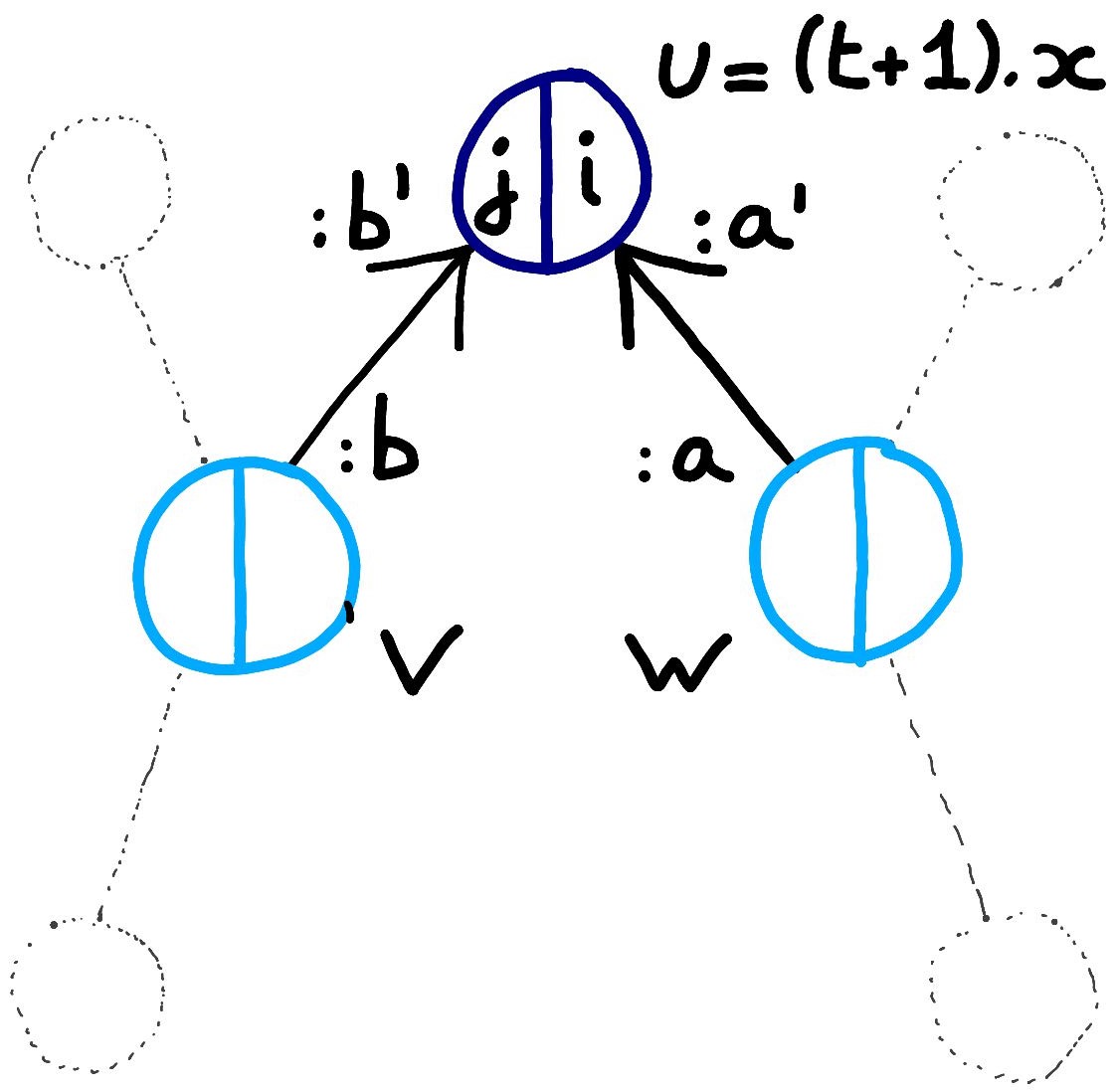
(b) $A_{x_{1}}G_{{\mathcal{N}_{x_{1}}}}$.

Figure 4: The local rule for the particle system. $A_{x}$ acts by consuming the internal state $i=\sigma^{r}_{G}(v)$ of vertex $v$ (and symmetrically with $j=\sigma^{l}_{G}(w)$), thereby moving those particles at $x$ if they are present. It also updates ports from $a,b$ to $a^{\prime},b^{\prime}$, flips the arrows pointing to $x$, and increments its timetag, in order to move the vertex from past $u=t.x$ to future $u^{\prime}=(t+1).x$. Dashed edges and vertices do not influence the local rule.

Definition 6 (Local rule)

A local rule is an operator over graphs $A_{(-)}:\mathcal{X}\to(\mathcal{G\to G})$ which is ${\mathcal{N}}$-local for some neighborhood scheme ${\mathcal{N}}$, i.e.

$$\forall G\in{\mathcal{G}},\forall x\in X(\mathrm{Past}(G)),\;A_{x}G=(A_{x}G_{\mathcal{N}_{x}})\sqcup G_{{\overline{\mathcal{N}}}_{x}}.$$

From now on $A_{yx}$ will stand for $A_{y}A_{x}$. We say that $\omega\in\mathcal{X}^{*}$ is a valid sequence in $G$ if, for all $\omega_{1},\omega_{2}\in\mathcal{X}^{*}$ such that $\omega=\omega_{2}x\omega_{1}$, we have $x\in X(\mathrm{Past}(A_{\omega_{1}}G))$. We denote $\Omega_{G}(A)\subseteq\mathcal{X}^{*}$ the set of valid sequences in $G$.

An additional property that can be required, without difficulty, of our operators, is renaming-invariance [24]. We will skip this here.

Remark 1

Notice that $A_{x}G$ must be well defined for any graph $G$. As a consequence, so must $A_{x}(G_{{\mathcal{N}_{\omega}}})\sqcup G_{\overline{{\mathcal{N}_{x}}}}$. This implies that :

• the border vertices $B_{G_{{\mathcal{N}_{\omega}}}}$ cannot be modified (dashed vertices in Fig. 3).

• the border edges $\mathrm{E}_{G_{{\mathcal{N}_{\omega}}}}\setminus\ (I_{G_{{\mathcal{N}_{\omega}}}}\!:\!\pi)^{2}$ cannot be modified (dashed edges in Fig. 3).

• new vertices $V_{A_{x}G}\setminus V_{G}$ are exclusively vertices in ${\scriptstyle\mathbb{Z}}.{\mathcal{N}^{-}_{x}(G)}$ with time tags increased by $A_{x}$ (the vertices in dark blue (e.g. $u_{1}$, $u_{2}$) in Fig. 3).

Now that we have a precise definition of the considered graphs and the kind of local transformations that we allow on them, let us state our goal informally. Consider a graph $G$, a local rule $A_{(-)}$ and all possible sequences $\omega,\omega^{\prime},\ldots\in\Omega_{G}(A)$. If one applies $A_{\omega}$, one obtains one possible evolution of the system. But $A_{\omega^{\prime}}$, $A_{\omega^{\prime\prime}}$,…are equally legitimate different orders of local rule applications. We aim to define precisely what it means for all these possible evolutions to actually agree on a consistent common story, i.e. a consistent space-time diagram. To motivate the remaining formalization, we consider examples. Later we give sufficient conditions for a local rule to induce such consistent space-time diagrams.

Definition 7 (Space-time diagram)

Given a graph $G$ and an local rule $A_{(-)}$, their space-time diagram $\mathcal{M}_{A}(G):=\{\,A_{\omega}G\mid\omega\in\Omega_{G}(A)\,\}$ is the set of all generated graphs. We sometime omit $A$ and $G$.

To visualize how the graphs in $\mathcal{M}$ share common vertices and edges, some space-time background are depicted (Figs 5, 6, and 8), each as pseudo-graph $M$ defined by :

$$V_{M}=\bigcup_{G\in\mathcal{M}}V_{G} E_{M}=\bigcup_{G\in\mathcal{M}}\mathrm{E}_{G}$$

and without internal states.

3 Particle system example

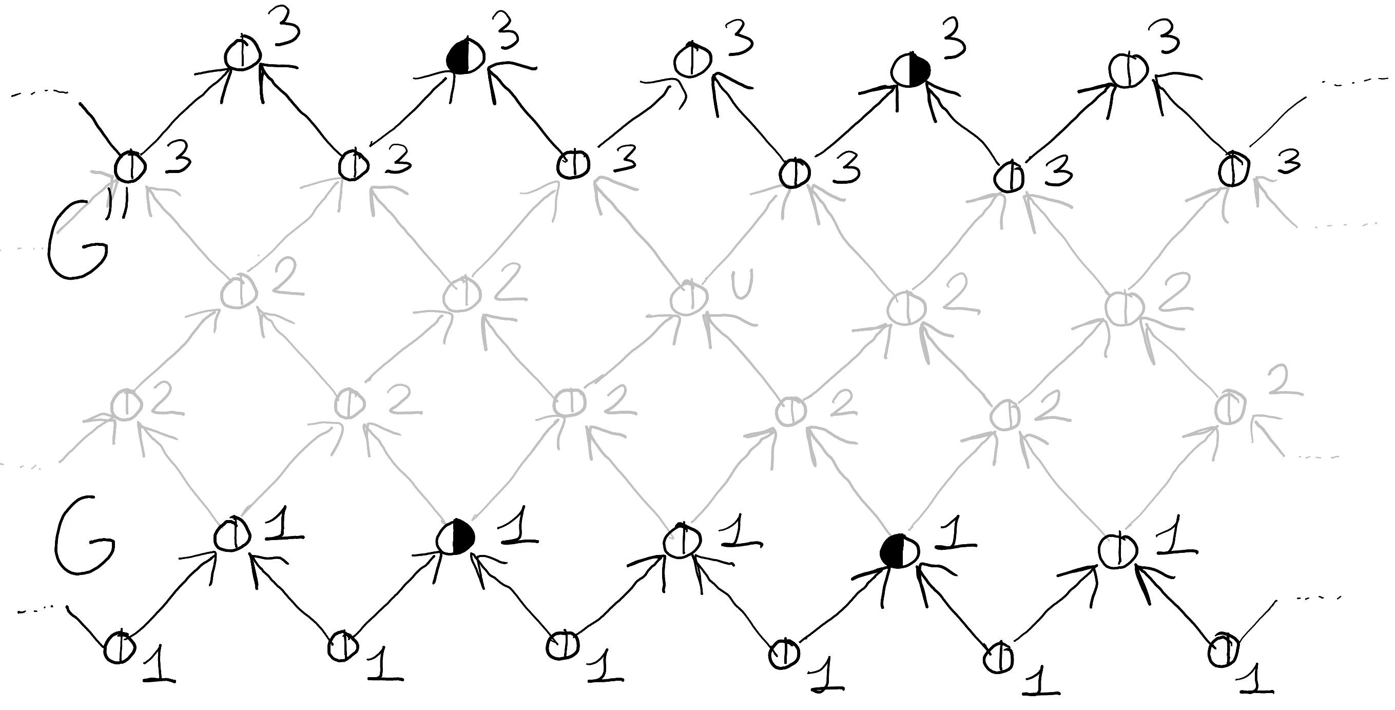
Figure 5: Particle system example. In black we highlight just the graphs $G$ and $G^{\prime\prime}$ belonging to the space-time diagram $\mathcal{M}(A,G)$. The local rule here moves the left-side particle towards the right and the right-side particle towards the left. Note how the problem raised by Fig. 1 is solved. The only point in space-time which can contain both particles is $u$.

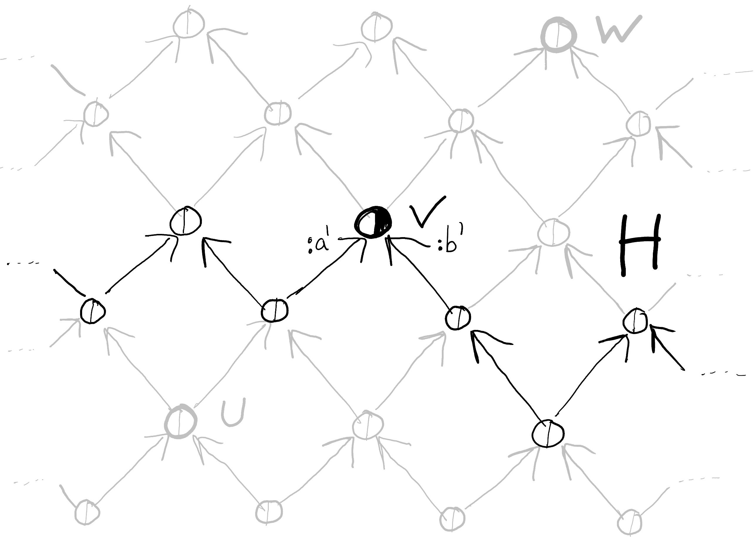
(a) Here $\sigma_{G}(v)=(0,1)$ $\dots$

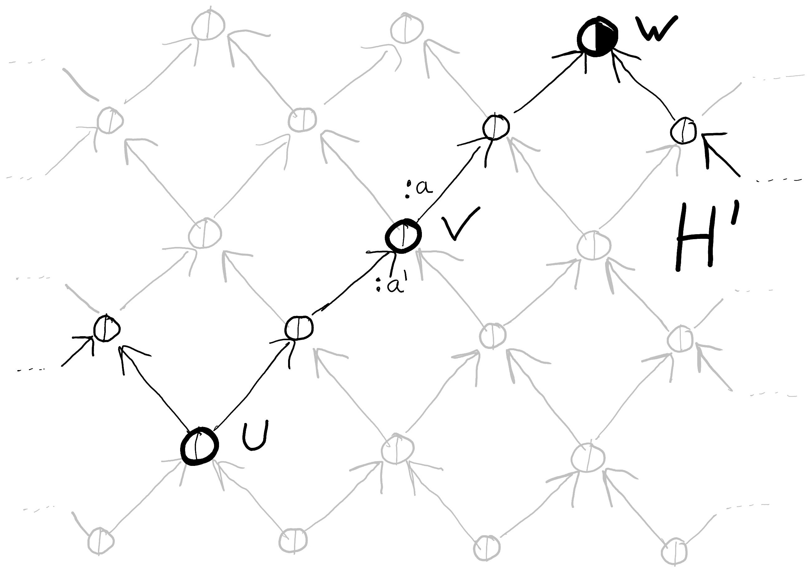
(b) $\dots$ whereas there $\sigma_{H}(v)=(0,0)$.

Figure 6: States depend on the cut. Both graphs $H$ and $H^{\prime}$ belong to the same space-time diagram $\mathcal{M}_{A}(H_{0})$ with $H_{0}$ containing a right-moving particle in $u$. They both contain vertex $v$. In $H^{\prime}$, the particle that was present in $H$ has moved to point $w$. The state associated to $v$ thus depends on the way it is cut, which is captured by its set of incoming ports e.g. $\{a^{\prime},b^{\prime}\}$ versus just $\{a^{\prime}\}$.

We now show how asynchronous applications of a local rule can represent a dynamical system of left and right moving particles, consistently, thereby fixing the issues of Fig. 1. The logic of this example borrows to the well-studied ‘marching soldiers’ scheme [25], as best formalised by [26]—although this particular instance taps on the reversibility of the dynamics for best state optimisation, and uses the DAG of dependency, rather than extra internal states, as its mechanism for local, relative synchronisation.
The vertices of our graphs have names of the form $u=t.x$, they must be thought of as events in space-time. The internal state of each vertex are pairs of bits $\sigma_{G}(u)=(\sigma^{l}_{G}(u),\sigma^{r}_{G}(u))$, representing the presence of a left-moving particle or not, and of a right-moving particle or not. The edges are oriented and go from port $:\!a$ to $:\!a^{\prime}$ or from port $:\!b$ to $:\!b^{\prime}$, thereby indicating a spatial direction ($a$ versus $b$) and a temporal orientation (unprimed versus primed). Altogether each graph must be thought of, not as a space-time diagram, but as a space-like cuts of a space-time diagram, see Fig. 5. In particular, they can never contain both vertices $u=t.x$ and $u^{\prime}=(t+1).x$. It follows that the local rule $A_{x}$ will act unambiguously on the unique vertex of the form $u=t.x$.
Edges must be thought of as dependencies between events, i.e. if $u=t.x$ points to $v=t^{\prime}.y$, then $v$ is ahead in time of $u$, and frozen awaiting for information from $u$. The action of $A_{y}$ on $v$ is therefore trivial, preventing $y$ to be computed too far ahead and providing a weak synchronisation mechanism. The action of $A_{x}$ on $u$ is non-trivial only if $u$ is minimal. Such a $u$ can be thought of as lagging behind in time, and no longer awaiting for any information—it has reached its local normal form. The action of $A_{x}$ is to dispose of it by communicating its information to $v$ and other dependencies, and creating vertex $u^{\prime}=(t+1).x$ in some provisional state. In our example this is done according to Fig. 4.
The local rules allow us to evolve one graph $G$, understood as a space-like cut, into another later space-like cut $G^{\prime\prime}$, as in Fig. 5. But the point is that the graph $G$ can also be evolved asynchronously into $H$ or $H^{\prime}$ as in Fig. 6. All of these graphs agree with each other with respect to the particle’s worldline. More generally, this local rule is space-time deterministic, it produces well-determined events. But notice that this property is a bit subtle to formulate, e.g. the state associated to the event $v$ seems different in $H$ and $H^{\prime}$, as the particle got ‘consumed’ from $v$ to $w$. The important point is that the state of every event $v$ (in terms of its internal state and connectivity) remains a function of how it is traversed in the space-like cut, which is here represented by its set of incoming ports. I.e. the example is fully consistent in the sense that the state of each vertex is fully determined by its set of incoming ports.
This ‘particle consumption mechanism’ of this example is a design choice, willingly taken in order illustrate three points: 1/ space-time determinism is really the idea that all events are well-determined, given the angle of their space-like-cut. E.g. in Physics the non-scalar quantum field associated to an event does depend on this angle. 2/ Ultimately this can be traced back to the nature of quantum information, which gets ‘consumed’ as it gets ‘read out’, because it cannot be ‘copied’. Our formalism is therefore compatible with the idea of linear evolutions, as will be required when we study reversible or quantum versions of these rules. 3/ The weak consistency criterion cares only for local normal vertices (aka Past), but in this example they are always empty (Figs 5 and 6). This suggests that weak consistency is too weak a conditions as it dangerously fails to capture the essence of this dynamical system: particles flying around. Altogether, this example shows that it is perfectly possible to consistently simulate a dynamical system by means of asynchronous rule applications. The aim sets the aim of the paper: to understand when asynchronism meets space-time determinism.

4 Time dilation example

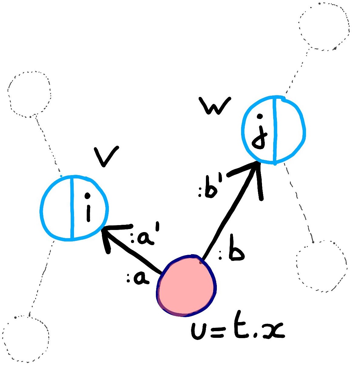
(a) $G_{{\mathcal{N}_{x}}}$.

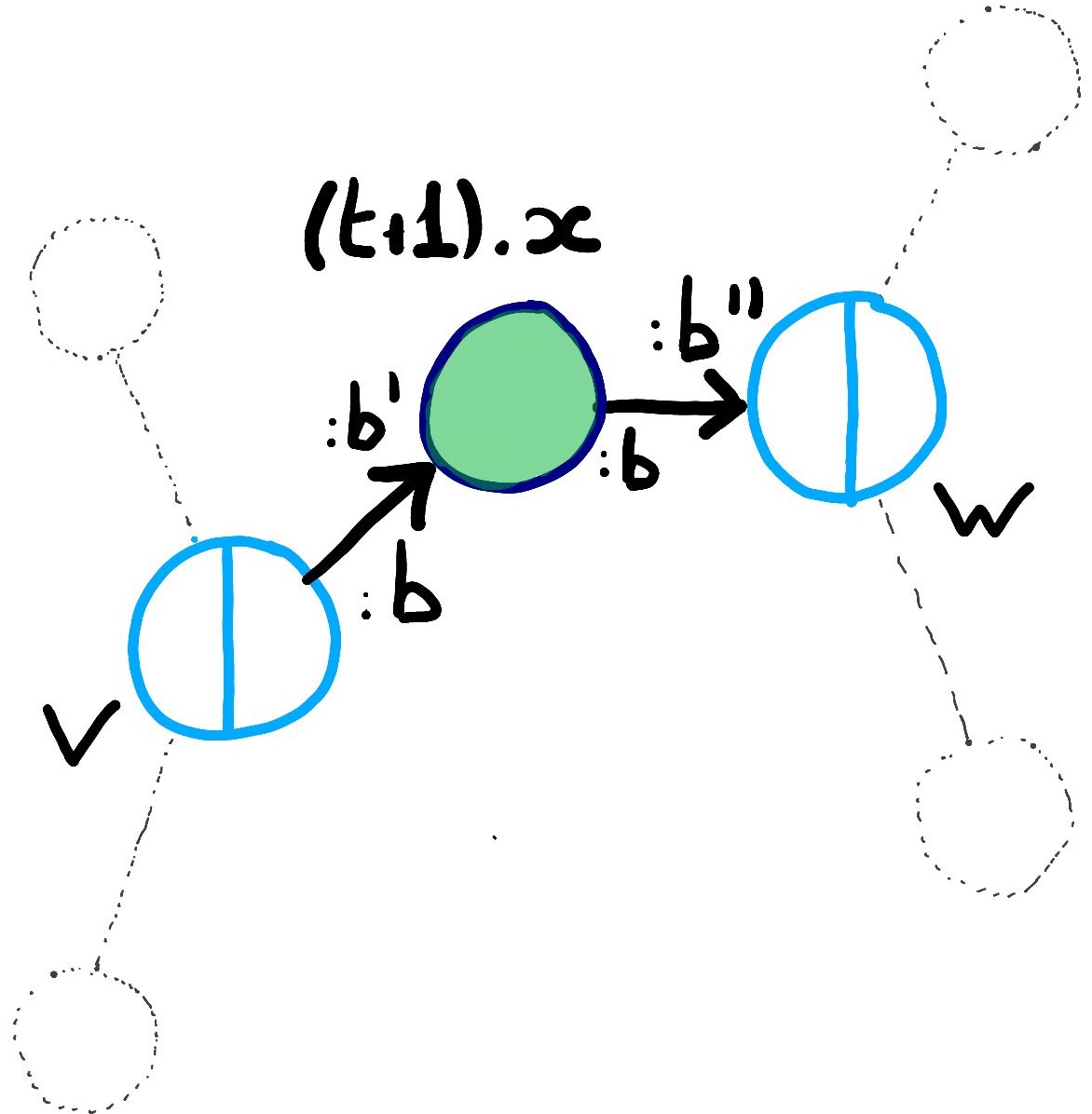
(b) $A_{x}(G_{{\mathcal{N}_{x}}})$.

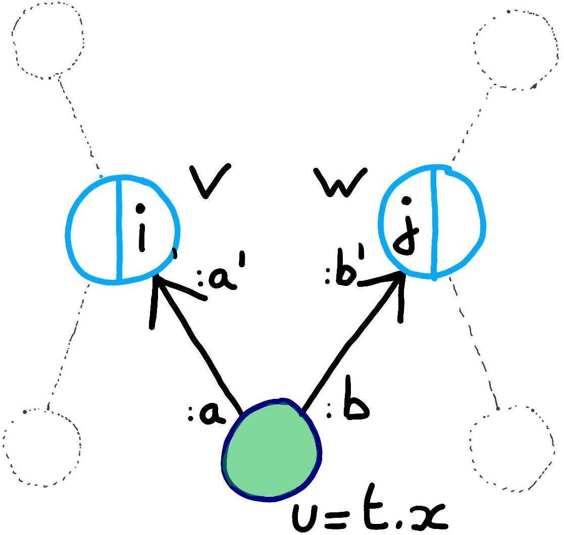
(c) $H_{{\mathcal{N}_{x}}}$.

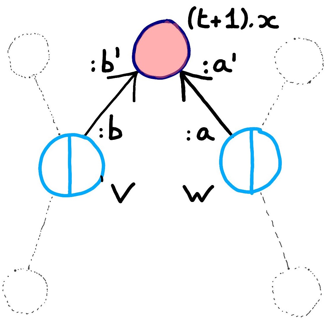
(d) $A_{x}(H_{{\mathcal{N}_{x}}})$.

Figure 7: The local rule for time dilation. We define here the behaviour of $A_{x}$ when $u=t.x$ is colored—i.e. $\sigma(u)=green\lor\sigma(u)=red$. In both cases particles get destroyed when reaching the colored vertex and we flip the color in $x$. When applied to a green vertex ($c$ & $d$) $A_{x}$ behaves as we are used to. When applied to a red vertex ($(a)$ & $(b)$) $A_{x}$ creates an anomaly. The edge between $(t+1).x$ and $w$ is reversed, thus we will be forced to apply $A_{x}$ again before updating $w$. Note that this evolution is still port-decreasing (see Def.12) because $b^{\prime}$ is replaced by a smaller port $b^{\prime\prime}$.

Our second example extends the internal state space $\Sigma$ used in Sec. 3 with two more states: the green and red states. The same local rule is extended so that if one such particle is found in position $x$, it will stay there, oscillating between both colours and altering the very texture of space-time as in Fig. 7. This results in time dilation as can be seen from Fig. 8: time ticks twice as slower on the right hand side of the red particle. Yet, the very same local rule is being applied left and right of the red particle. Such a phenomenon is reminiscent of general relativity, e.g. time flows slower on Earth than it does in the stratosphere, as measured by identically made clocks. Yet, the same laws of Physics apply in the stratosphere and on Earth. How did we get there?

Maybe this is not quite a coincidence. To some extent, the construction of this model mimics some of the key steps of the construction of general relativity as derived from physical symmetries. Indeed, let us remind the reader that the standard derivation proceeds by: 1/ Assuming the existence of a well-determined space-time. 2/ Requiring covariance, i.e. invariance under changes of coordinates, which in particular implies a form of asynchronism as one can choose coordinates whereby one region of a space-like cut will evolve (large time lapse), but not the other (small time lapse). 3/ Concluding that in order to obtain covariance, one needs to provide extra causality structure at each point, namely the metric field. 4/ Assuming background-invariance, namely enabling the possibility that space-time be curved by the presence of this newly allowed metric. 5/ Providing a dynamic upon the metric itself.
Here, in the discrete, we: 1/ enforced a well-determined space-time, 2/ in spite of an asynchronous evaluation strategy, 3/ thanks to the introduction of extra causality structure, namely a DAG of dependencies. 4/ We then allowed ourselves to consider graphs with exotic such DAG, and 5/ rules manipulating them.

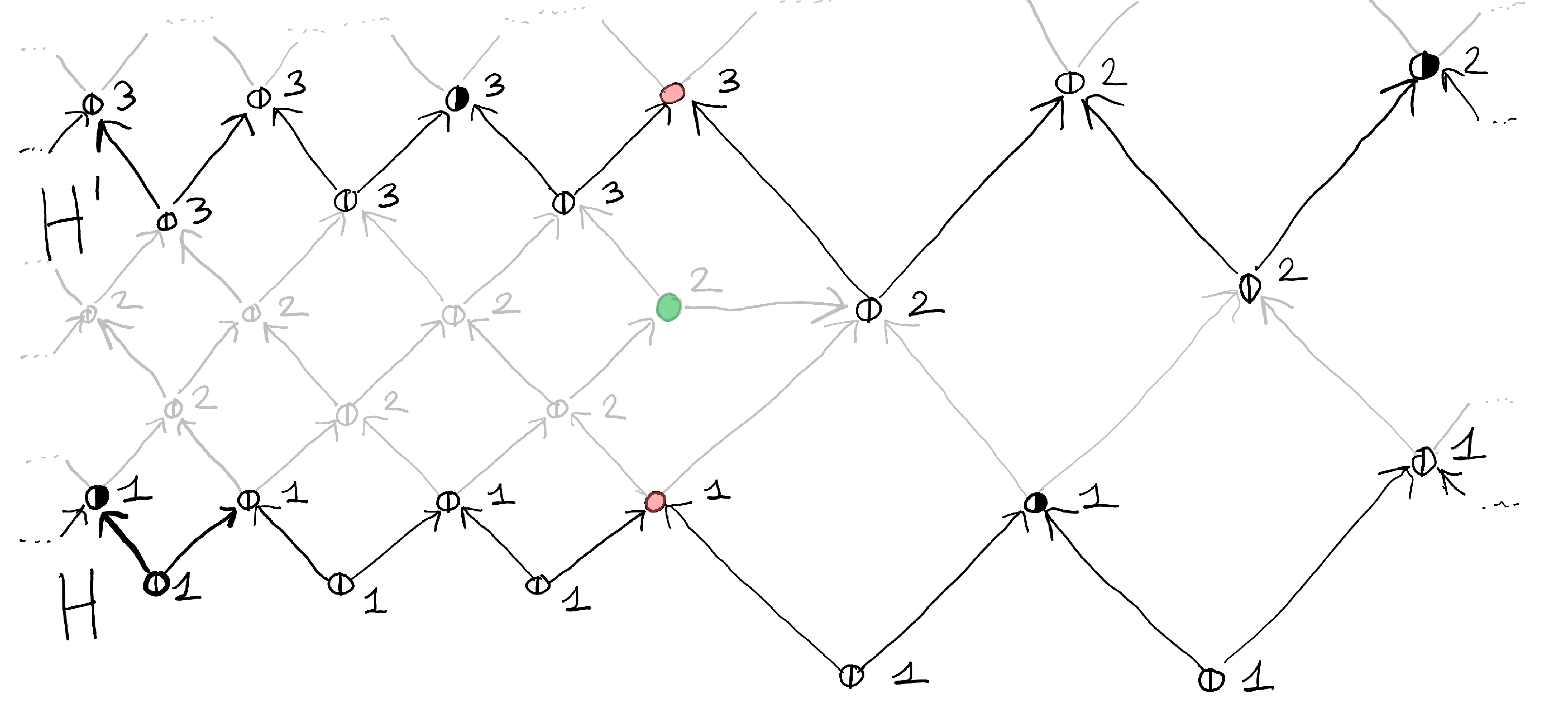
Figure 8: Time dilation example. In black we highlight two graphs $G$ and $G^{\prime\prime}$ belonging to the space-time diagram. We start with two particles, one on the left and the other on the right of the red. Notice how, even if the same local rule gets applied everywhere, times flows twice faster for the particle on the left.

5 Obtaining space-time determinism

One might have hoped for a simple definition of space-time determinism, whereby any two graphs of a space-time diagram $\mathcal{M}$ must agree on the state of a vertex $u\in{\mathcal{V}}$, if it so happens to appear in both of them. But the example in Sec. 3 (Fig. 6) shows that things are more subtle. Its discussion motivates a definition of (full) consistency whereby any two graphs of $\mathcal{M}$ must agree on the state of a vertex $v$ (in terms of its neighbourhood and internal state) whenever they agree on the set of incoming ports to that vertex $v$. In particular this implies that the state of $v$ should be the same for every graph of $\mathcal{M}$ such that $v\in\mathrm{Past}(G)$, which can be understood as stating that the “result state” (a.k.a. normal form) at $v$ is well-determined. We refer to this weaker demand as weak consistency (see Fig. 9).

Definition 8 (Consistency)

Two graphs $G$ and $H$ are consistent iff for all $v\in\mathrm{I}_{H}\cap\mathrm{I}_{G}$:

$$\pi.\mathrm{E}_{G}(v)=\pi.\mathrm{E}_{H}(v)\Longrightarrow G_{v}=H_{v}.$$

where $\mathrm{E}_{G}(v)$ the set of edges ending in $v$, and $\pi.\mathrm{E}_{G}(v)$ denotes the set of incoming ports of $v$. Consistency is denoted $G\varparallel H$. The graphs $G$ and $H$ are called weakly consistent if they respect this condition in the special case where $\mathrm{E}_{G}(v)=\emptyset$. We say that a space-time diagram $\mathcal{M}$ is (resp. weakly) consistent if each pair of graphs in $\mathcal{M}$ is (resp. weakly) consistent.

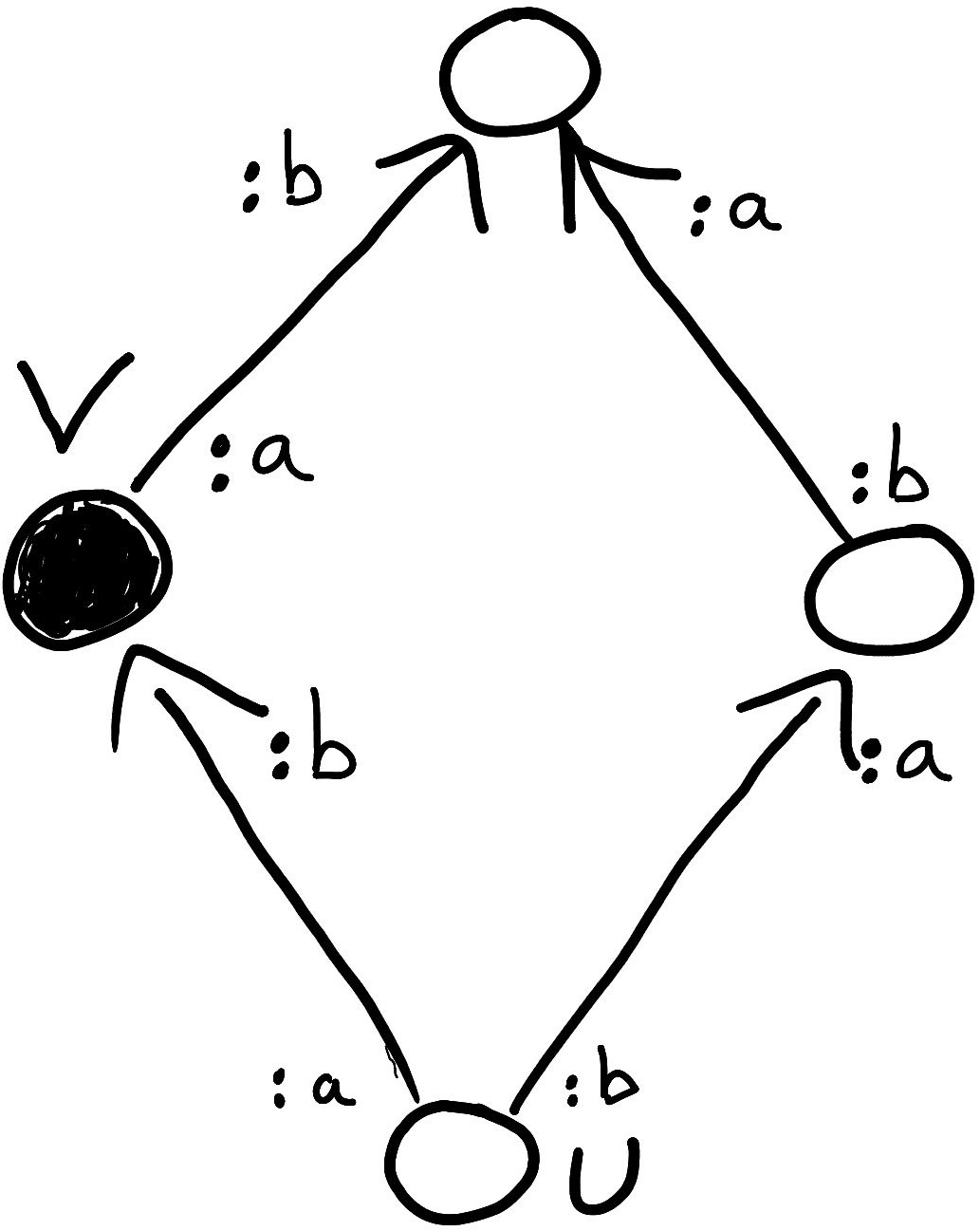
(a) $G$

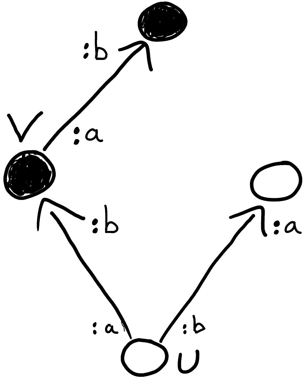
(b) $H$

Figure 9: Weak consistency versus consistency. The set of graphs $\{G,H\}$ is weakly consistent but not consistent. Indeed we have $G_{u}=H_{u}$ but consistency fails in $v$ because we have $\mathrm{E}{G}(v)=\mathrm{E}{H}(v)$ but $G_{v}\neq H_{v}$. As a consequence (see Prop. 2) we have $G\neq H$ whilst $\mathrm{Past}(G)=\mathrm{Past}(H)$.

We now embark in the quest for a set of properties ensuring that an ${\mathcal{N}}$-local rule $A_{(-)}$ generates only consistent space-time diagrams. We start with two properties. The first one asks for timetags to only increase. The second one, akin to strong confluence or sequential independence in parallel graph transformations, states that a set of independent rule applications on a graph $G$ applied in any order should always lead to the same graph.

Definition 9 (Time-increasing commutative local rules)

A local rule $A_{(-)}$ is

• time-increasing iff $\forall t.y\in V_{G},\,\forall t^{\prime}.y\in V_{A_{x}G},\;t\leq t^{\prime}\text{, with }t<t^{\prime}\textit{ if }y=x$;

• commutative iff $\forall x,y\in X(\mathrm{Past}(G)),\;A_{x}A_{y}(G)=A_{y}A_{x}(G)$.

These two properties place strong constraints on the past vertices of a space-time diagram $\mathcal{M}_{A}(G)$: they already entail weak consistency. Moreover each space-like cut is fully determined its set of past elements.

Proposition 1 ()

(Obtaining weak consistency). Let $A_{(-)}$ be a time-increasing commutative local rule. For all graph $G$, $\mathcal{M}_{A}(G)$ is weakly consistent.

Proposition 2 ()

(Pasts determine space-like cuts) Let $A_{(-)}$ be a time-increasing commutative local rule. Let $G$ be a graph. Let $H,J\in\mathcal{M}_{A}(G)$. If $\mathrm{Past}(J)=\mathrm{Past}(H)$ then $J=H$.

However Sec. 3 discussed how weak consistency can be trivially realised even for non-trivial dynamics, and justified going for full consistency. To have sufficient condition for full consistency, we place new hypotheses on the neighbourhood scheme, namely extensivity, monotony and privacy.

Note that all this properties are respected by the neighbourhood ${\mathcal{N}}$ used in examples of Secs 3 and 4 defined by :

$$\forall x\in\mathcal{X},\mathcal{N}_{x}(G)=\mathrm{V}_{G_{x}} \forall\omega\in\mathcal{X}^{*},\mathcal{N}_{\omega}(G)=\bigcup_{x\in\omega}\mathcal{N}_{x}(G)$$

First we demand that $\mathcal{N}_{\omega}(G)$ be big enough to contain the neighbourhood of each vertex $x\in\omega$, at the time $A_{x}$ is to be computed. This closure property of ${\mathcal{N}}$ is called monotony (see Fig.10), it ensures that for any valid sequence $\omega$, $A_{\omega}$ will not modify beyond $\mathcal{N}_{\omega}(G)$.

Definition 10 (Monotony)

A neighbourhood scheme ${\mathcal{N}}$ is monotonous iff for every sequence $\omega=\gamma\beta\alpha\in\Omega_{G}(A)$ we have :

$$\mathcal{N}_{\beta}(A_{\alpha}G)\subseteq\mathcal{N}_{\omega}(G).$$

In particular we have $\mathcal{N}_{\beta}(A_{\alpha}G)\subseteq\mathcal{N}_{\beta\alpha}(G)$ and $\mathcal{N}_{\alpha}(G)\subseteq\mathcal{N}_{\omega}(G)$.

Second, privacy will demand that any disjoint sequences $\omega,\omega^{\prime}$ have their $\mathcal{N}_{\omega}(G)$ and $\mathcal{N}_{\omega^{\prime}}(G)$ intersecting only on their border vertices and the edges in between them (see Fig. 10), a property that is akin to parallel independence [13]. Combining the two together will ensure that concurrent influences happen only at these joint borders, an essential ingredient of full consistency, as illustrated in Fig. 11(a) and 11(b)).

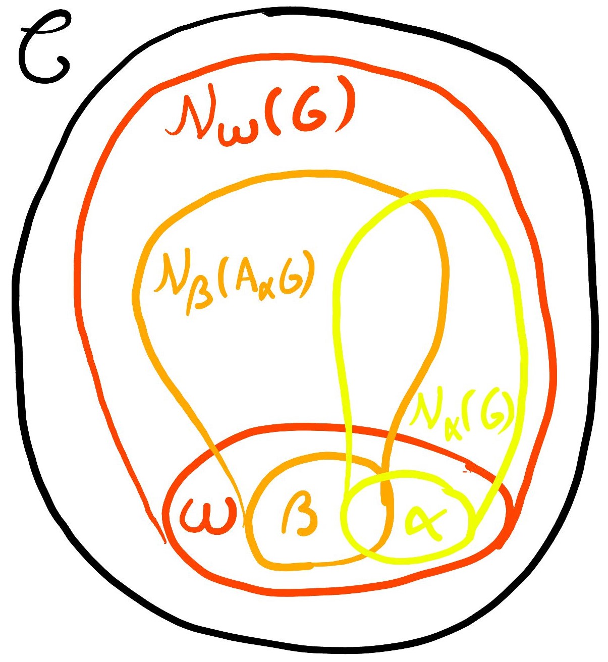
(a) Monotony.

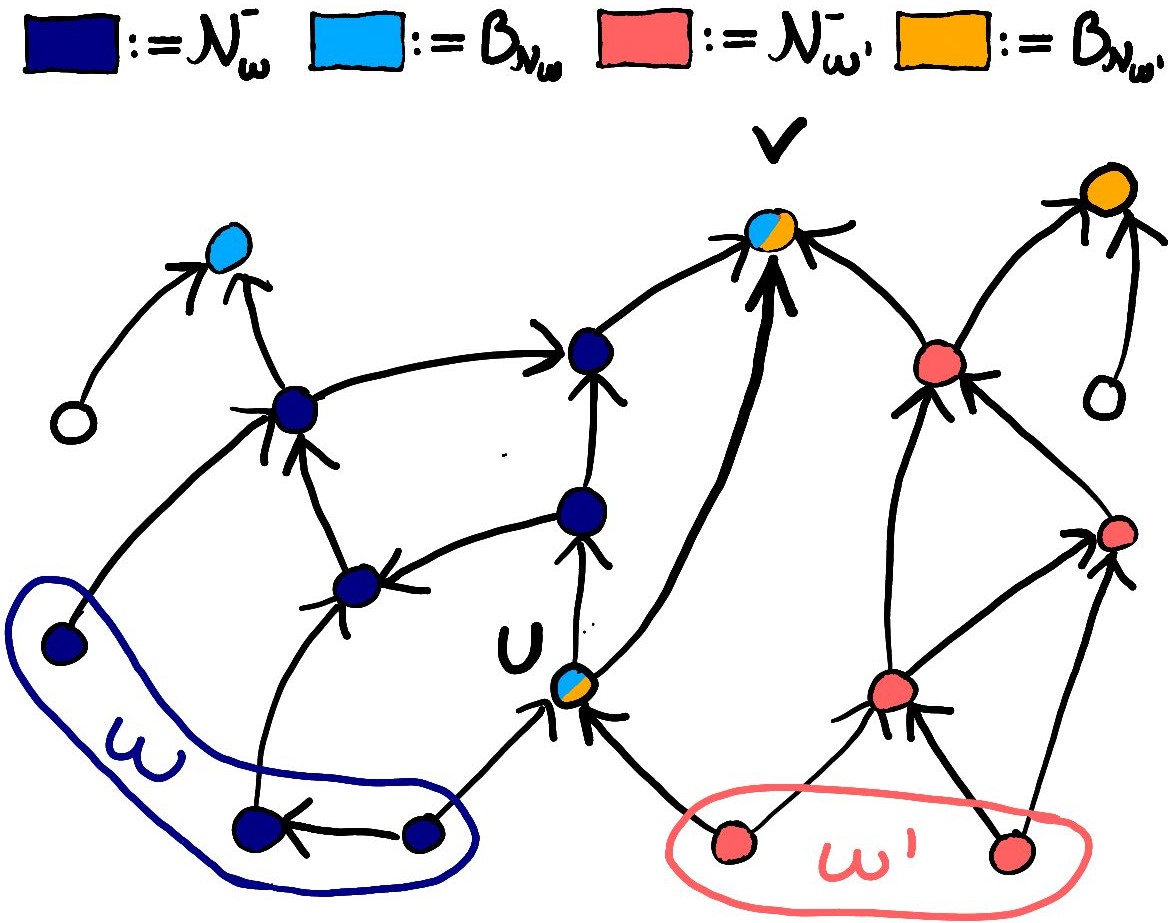
(b) Privacy and port decreasing.

Figure 10: Monotony and privacy. $(a)$ The monotony condition demands that given a graph $G$ and a list of vertices $\omega=\beta\alpha$ monotony demands that the neighbourhood computed at the beginning ${\mathcal{N}_{\omega}}(G)$ (red) is larger that ${\mathcal{N}}_{\alpha}(G)$ (yellow) and that any future neighbourhood ${\mathcal{N}}_{\beta}(A_{\alpha}G)$ (orange). Given a set of disjoint vertices $\omega^{\prime}$ privacy demands that the neighbourhood ${\mathcal{N}_{\omega}}$ (blue & cyan) and ${\mathcal{N}}_{\omega^{\prime}}$ (red & orange) only intersect on their borders. $(b)$ The port decreasing condition demands that, in order to modify a vertex, $A_{\omega}$ must pay the price of decreasing one of its incoming private ports. Here, $x\in G_{{\mathcal{N}_{\omega}}}\cap G_{{\mathcal{N}_{\omega^{\prime}}}}$ can be modified by both $A_{\omega}$ and $A_{\omega^{\prime}}$ as each of them has private access to it.

Definition 11 (Privacy)

A neighbourhood scheme ${\mathcal{N}}$ is private, iff for any graph $G$ and any disjoint valid sequences $\omega,\omega^{\prime}\in\Omega_{G}(A)$, we have :

$${\mathcal{N}^{-}_{\omega^{\prime}}(G)}\cap\mathcal{N}_{\omega}(G)=\emptyset.$$

Lastly we want to forbid that a local rule modifies a vertex without altering its incoming ports, as this would immediately infringe full consistency (see Fig. 11(c) and 11(d)). Moreover the modification needs be decreasing—otherwise we could apply $A_{x}$ twice in a row and get to the exact same counter example. This idea that $A_{x}$ should decrease the incoming ports of the vertex $v$ it modifies, can be understood as a natural way of ‘locally reflecting the progress of the computation of $v$’, i.e. geometrically accounting for the fact that the dependency between $x$ and $v$ has been reduced, and hence their space-time relationship has changed. In Sec. 3 the local rule is port decreasing because we suppress an incoming edge each time we modify a vertex. In Sec. 4 the local rule is port decreasing for more subtle reasons in the case of a red vertex : we decrease $b^{\prime}$ into $b^{\prime\prime}$ (see Fig. 7(a) and 7(b)).

Definition 12 (Port decreasing)

An ${\mathcal{N}}$-local rule $A_{(-)}$ is port decreasing iff for any graph $G$, position $x\in X(\mathrm{Past}(G))$ and vertex $u\in V_{G}\cap V_{A_{x}G}$ whenever $G_{u}^{0}\neq(A_{x}G)_{u}^{0}$ we have

$$\pi.(\mathrm{E}_{G}(V_{G},u)\setminus\mathrm{E}_{G}({\overline{\mathcal{N}^{-}_{\omega}}},u))>\pi.(\mathrm{E}_{A_{x}G}(V_{A_{x}G},u)\setminus\mathrm{E}_{G}({\overline{\mathcal{N}^{-}_{\omega}}},u))$$

for a order $\leq$ over sets of ports which is for any $A,B,A^{\prime},B^{\prime}\in\mathcal{P}(\pi)$ :

• inclusive i.e. $A\supseteq A^{\prime}\Longrightarrow A\geq A^{\prime}$

• monotonous i.e. $A\cap B=\emptyset\ \land\ A\geq A^{\prime}\ \land\ B>B^{\prime}\Longrightarrow A\cup B>A^{\prime}\uplus B^{\prime}$

where $\mathrm{E}_{G}(Y,u)$ denotes the set of edges in $G$ from any $v\in{\scriptstyle\mathbb{Z}}.Y$ to $u$, and $\pi.\mathrm{E}_{G}(Y,u)$ the corresponding set of ports incoming to $u$.

Note that we ask a port decreasing operator to decrease the port of a private edge, i.e. an edge starting from ${\mathcal{N}}^{-}$. Without this assumption we can give a counter example by considering the graph of Fig. 10. Say both $A_{\omega}$ and $A_{\omega^{\prime}}$ were to modify the internal state of $v$ and decrease the port associated to the shared edge coming from $u$. Then we could have $\pi.\mathrm{E}_{A_{\omega}G}(v)=\pi.\mathrm{E}_{A_{\omega^{\prime}}G}(v)$ whilst $\sigma_{A_{\omega^{\prime}}G}(v)\neq\sigma_{A_{\omega}G}(v)$.

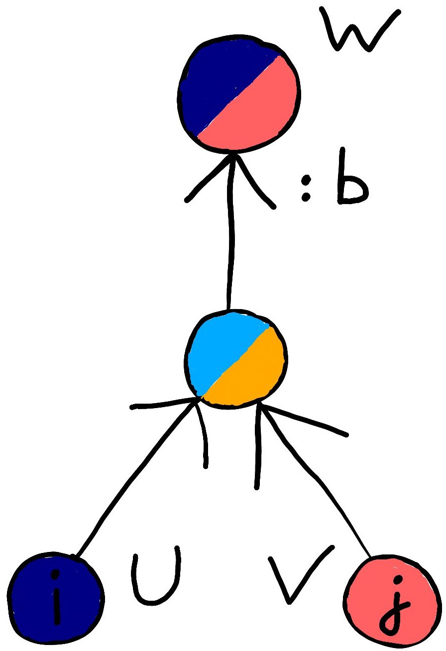
(a) $G$

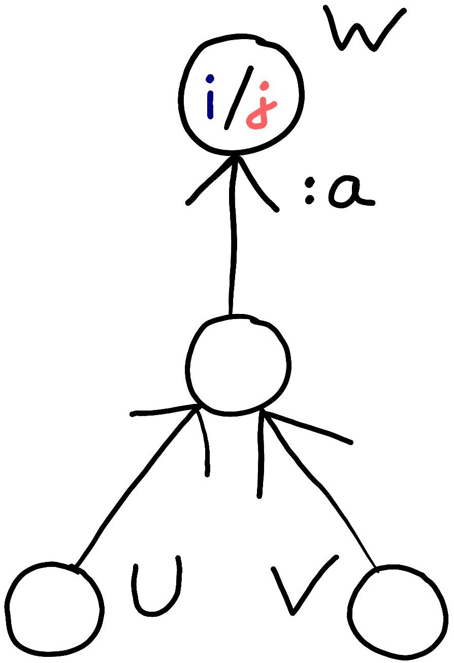
(b) $A_{u}G$/$A_{v}G$

(c) $G$

(d) $A_{u}G$

Figure 11: Inconsistent dynamics examples. The example of $(a)\&(b)$ relies on a neighbourhood scheme which is not private as $w\in{\mathcal{N}^{-}_{u}(G)}\cap{\mathcal{N}^{-}_{v}(G)}$. It follows that $A_{u}G$ and $A_{v}G$ disagree on the internal states of $w$, whilst both updating its incoming port in the same fashion ($b$ becomes $a<b$). The example of $(c)\&(d)$ is not port decreasing. It follows that $G$ and $A_{u}G$ disagree on $v$ but its set of incoming ports stay the same.

Finally we state our main result.

Theorem 5.1 ()

(Obtaining consistency) Let $A_{(-)}$ be a port-decreasing time-increasing commutative ${\mathcal{N}}$-local rule, with ${\mathcal{N}}$ an extensive monotonous and private neighbourhood scheme. For all graph $G$, $\mathcal{M}_{A}(G)$ is consistent.

The proof is quite intricated, but we can give the following intuition. On the one hand the commutation hypothesis ensures that $A_{\omega}G\varparallel A_{\omega^{\prime}}G$ as long as $\omega^{\prime}$ is a permutation of $\omega$. On the other hand as long as ${\mathcal{N}}$ is extensive, monotonous and private two disjoint operators necessarily modify different subgraphs, albeit with a common border. Then, by decreasing the private incoming port of each modified vertex, we obtain full consistency by dismissing its premise.

6 Conclusion

Summary of results. We introduced graphs that must be thought of as a space-like cuts of space-time diagrams. The vertices have names of the form $u=t.x$, they must be thought of as events. The edges must be thought of as dependencies between events, i.e. if $u=t.x$ points to $v=t^{\prime}.y$, then $v$ is ahead in time of $u$, awaiting for information from $u$. The action of a local rule $A_{x}$ on $u$ is non-trivial only if $u$ is minimal: it disposes of it by communicating its information to $v$ and other dependencies, and creates vertex $u^{\prime}=(t+1).x$ in some provisional state.
We argued that the right notion of space-time determinism is full consistency: the state of each event (in terms of its internal state and connectivity) needs be a function of its set of incoming ports, as these represent the angle at which the space-like cut traverses the event. We gave sufficient conditions for the asynchronous applications of a local rule to be fully consistent: they must be commuting and port-decreasing, with respect to an extensive, monotonous, private notion of neighbourhood. We also looked at a weaker notion of consistency, requiring that only the normal forms of events across space-time be well-determined: commutation alone suffices then.
Throughout, we argued of the potential implications for distributed computation (weak consistency), asynchronous simulation of dynamical systems (full consistency and our first example), and discrete toy models of general relativity (our second example).

Related works. Geometry is dynamical in a our work. We thus hope it makes useful addition to the already wide literature on Graph Rewriting [27, 28]. We are aware that the dominating vocabulary to describe them is now that of Category theory [29, 30, 23], in which ways of combining non-commuting rules [31] and notions of space-time diagrams have been developed [32, 33, 34, 35].
We instead use the vocabulary of dynamical systems, as we came to consider Graph Rewriting though a series of works generalising cellular automata to synchronous, causal graph dynamics [36], and tilings to graph subshifts [37]. We are confident that abstracting away the essential features of our formalism could yield interesting categorical frameworks, e.g. à la [38].
The closest works however turn out to come from varied communities. In algorithmic complexity [39] uses a DAG of dependencies representation to reduce the synchronisation costs of simulating a class of synchronous algorithms—we use it in the more dynamical systems context and in order to relax synchronism altogether, whilst safeguarding space-time determinism. In computational Physics [40] promotes the lattice of dependencies of local rule applications to a notion space-time, and advocates a notion of ‘causal invariance’ based on the unicity of this lattice—we formalise space-determinism mathematically and provide local conditions to achieve it. In the network reliability community, [25] obtains a result of a similar flavour to Prop. 1—our local rules $A_{x}$ are allowed to modify the neighbouring nodes and the graph per se, plus we reach full consistency.

Perspectives. Clock synchronisation is an expensive overhead for parallel simulation of dynamical systems, as well as numerous distributed computation applications. The hereby developed theoretical framework says we can just do away with them and still obtain a strong form space-time determinism, provided that the local rule meets certain requirements. We are looking forward to see this being applied in practice. We, on the other hand, are likely to focus on the reversible and quantum regimes of these graph rewriting models.

Acknowledgements  We wish to thank Nicolas Behr for helpful discussions. This publication was made possible through the support of the PEPR integrated project EPiQ ANR-22-PETQ-0007 part of Plan France 2030, and the ID #62312 grant from the John Templeton Foundation, as part of the ‘The Quantum Information Structure of Spacetime’ Project (QISS) . The opinions expressed in this project/publication are those of the author(s) and do not necessarily reflect the views of the John Templeton Foundation.

Appendix 0.A Valid sequences and commutative local-rule

We notice that a past vertex must remains so, hence the well-definiteness of commutativity.

Lemma 1 (Validity of community)

Let $A$ be a (not necessarily commutative) local rule, $G$ be a graph and $x,y\in X(\mathrm{Past}(G))$. The sequence $yx$ is valid in $G$. Moreover, if A is commutative, $A_{xy}G=A_{yx}G$.

Proof

As there exists no path to $y$ in $G$, the reachability condition of neighbourhood schemes implies that $y\notin\mathcal{N}_{x}(G)$. By ${\mathcal{N}}$-locality $A_{x}$ cannot add any incoming edge to $y$ which implies $y\in X(\mathrm{Past}(A_{x}G))$, i.e. $yx$ is valid as wanted.

Lemma 2 (*-validity of commutativity)

Let $A$ be a commutative local rule. Let $\alpha$ be a valid sequence in $G$. Let $x\in X(\mathrm{Past}(G))$ such that $x\notin\alpha$. We have $x\alpha$ and $\alpha x$ are valid in $G$ and $A_{x\alpha}G=A_{\alpha x}G$.

Proof

We proceed by induction on the size of $\alpha$. When $|\alpha|=0$ it is immediate. Let us suppose $\alpha=y\beta$. By induction hypothesis, we known that (1) $x\beta$ is valid in $G$, (2) $\beta x$ is valid in $G$ and (3) $A_{x\beta}G=A_{\beta x}G$. By (1), we have $x\in X(\mathrm{Past}(A_{\beta}G))$. Since $\alpha=y\beta$ is supposed to be valid, we also have $y\in X(\mathrm{Past}(A_{\beta}G))$. But Lem. 1 tells us that $xy$ and $yx$ are both valid in $A_{\beta}G$ and $A_{xy}(A_{\beta}G)=A_{yx}(A_{\beta}G)$. Thus $xy\beta$ and $yx\beta$ are valid in $G$ and $A_{xy\beta}G=A_{yx\beta}G=A_{y}(A_{x\beta}G)$. Combining this with (2) and (3) finishes the induction and the proof.

The two-letters commutativity condition is equivalent the ability to permute all letters of a valid sequence.

Lemma 3 ($*$-commutation)

Let $A_{(-)}$ be a commutative local rule. Let $\omega$ be a valid sequence in $G$ and $\omega^{\prime}$ be a permutation of $\omega$ also valid in $G$. We have

$$A_{\omega}G=A_{\omega^{\prime}}G$$

Proof

Let us denote $\omega=x_{n}\dots x_{2}x_{1}$. We prove by induction that for all $i\in\{0,\dots,n\}$,

$$A_{\omega^{\prime}}G=A_{\beta}A_{x_{i}\dots x_{1}}G,$$

with $\beta$ a permutation of $x_{n}\dots x_{i+1}$. The case $i=0$ is verified with $\beta=\omega^{\prime}$. When $i=j+1$ we have $A_{\omega^{\prime}}G=A_{\beta}A_{x_{j}\dots x_{1}}G$. By validity of $\omega$, we know that $x_{j+1}\in X(\mathrm{Past}(A_{x_{j}\dots x_{1}}G))$. Consider the decomposition $\beta=\beta^{\prime\prime}x_{j+1}\beta^{\prime}$ with $x_{j+1}\notin\beta^{\prime}$. Lem. 2 applied to $\beta^{\prime}$ and $x_{j+1}$ in the graph $A_{x_{j}\dots x_{1}}G$ gives us $A_{\omega^{\prime}}G=A_{\beta^{\prime\prime}\beta^{\prime}}A_{x_{j+1}\dots x_{1}}G$ as needed to finish the induction.

Appendix 0.B Weak consistency

For the next proof we will need a notation for the rightmost sequence subtraction. Let $\omega\in\mathcal{X}^{*}$ and $\alpha\in\mathcal{X}^{*}$. We define recursively $(\omega\setminus\alpha)\in\mathcal{X}^{*}$ as :

$$\omega\setminus\alpha=\begin{cases}\omega&\text{if }|\alpha|=0,\\ \omega^{\prime\prime}\omega^{\prime}&\text{if }|\alpha|=1,\omega=\omega^{\prime\prime}\alpha\omega^{\prime},\text{ and }\alpha\notin\omega^{\prime}\\ (\omega\setminus x)\setminus\alpha^{\prime}&\text{if }\alpha=\alpha^{\prime}x\text{ and }x\in\mathcal{X}.\end{cases}$$

For example if $\mathcal{X}=\{0,\dots,9\}$, $\omega=22159892$ and $\omega^{\prime}=28542$ we have $\omega\setminus\omega^{\prime}=2199$. This operation preserves validity.

Lemma 4 (Validity of sequence substraction)

Let $A_{(-)}$ be a commutative local rule. Let $\omega$ and $\omega^{\prime}$ be valid sequences. Then the sequence $\omega\setminus\omega^{\prime}$ is valid in $A_{\omega^{\prime}}G$.

Proof

We proceed by induction on the size of $\omega^{\prime}$. It is immediate when $\omega^{\prime}$ is empty. When $\omega^{\prime}=x\alpha$, the validity of $\omega^{\prime}$ gives us that $x\in X(\mathrm{Past}(A_{\alpha}G))$. The induction hypothesis is that $\omega\setminus\alpha$ is valid in $A_{\alpha}G$. Taking $\omega\setminus\alpha=\gamma\beta$ with $\beta$ the longest suffix of $\omega\setminus\alpha$ such that $x\notin\beta$, we have $\beta$ valid in $A_{\alpha}G$.

We can use Lem. 2 on $\beta$ and $x$ in $A_{\alpha}G$ to get validity of $\beta$ in $A_{x\alpha}G$ and $A_{x\beta\alpha}G=A_{\beta x\alpha}G$. If $\gamma=\varepsilon$ we can conclude immediately. Otherwise we have $\gamma=\beta^{\prime}x$. Since $\beta^{\prime}$ is valid in $A_{x\beta\alpha}G$ it is also valid in $A_{\beta x\alpha}G$. This finishes to prove validity of $\beta^{\prime}\beta=\omega\setminus x\alpha$ in $A_{x\alpha}G$.

Whilst confluence is not the primary aim of this paper, we obtain it as a corollary.

Corollary 1 (Confluence)

Let $A_{(-)}$ be a commutative local rule. Let $\omega$ and $\omega^{\prime}$ be valid sequences. Then the sequences $\omega^{\prime}\setminus\omega$ and $\omega\setminus\omega^{\prime}$ are valid respectively in $A_{\omega}G$ and $A_{\omega^{\prime}}G$. This enforces :

$$A_{(\omega^{\prime}\setminus\omega)}A_{\omega}G=A_{(\omega\setminus\omega^{\prime})}A_{\omega^{\prime}}G$$

Proof

We get each validity by one application of Lem. 4. Then we get the equality by applying Lem. 3.

In any spacetime diagram ${\cal M}_{A}(G)$ for $A$ time-increasing commutative, the state of a past vertex is well-determined.

Lemma 5 (Common past vertices have been equally updated)

Let $A_{(-)}$ be a time-increasing commutative local rule. Let $\omega$ and $\omega^{\prime}$ be valid sequences in $G$. If there exists $t.x\in\mathrm{Past}(A_{\omega}G)\cap\mathrm{Past}(A_{\omega^{\prime}}G)$ then $\omega^{\prime}$ contains as much $x$ as $\omega$.

Proof

We suppose without loss of generality that there is at least as much $x$ in $\omega^{\prime}$ than in $\omega$. Then because $x\notin(\omega\setminus\omega^{\prime})$ and $t.x\in\mathrm{Past}(A_{\omega^{\prime}}G)$ we have $t.x\in\mathrm{Past}(A_{(\omega\setminus\omega^{\prime})\omega^{\prime}}G)$. Using Lem. 1 this implies $t.x\in\mathrm{Past}(A_{(\omega^{\prime}\setminus\omega)\omega}G)$. Since $t.x\in\mathrm{Past}(A_{\omega}G)$ this implies by the time-increasing condition that $\omega^{\prime}\setminus\omega$ does not contain any $x$.

See 1

Proof

Let $\omega$ and $\omega^{\prime}$ be valid sequences in $G$. Let $t.x\in\mathrm{Past}(A_{\omega}G)\cap\mathrm{Past}(A_{\omega^{\prime}}G)$. Lem. 5 tells us that there is as much $x$ in $\omega^{\prime}$ than in $\omega$. This means $x\notin(\omega\setminus\omega^{\prime})$ and $x\notin(\omega^{\prime}\setminus\omega)$. Then, using locality and Lem. 1, we get the following equalities

$$(A_{\omega^{\prime}}G)_{t.x}=(A_{(\omega\setminus\omega^{\prime})\omega^{\prime}}G)_{t.x}=(A_{(\omega^{\prime}\setminus\omega)\omega}G)_{t.x}=(A_{\omega}G)_{t.x}.$$

Moreover, in any spacetime diagram ${\cal M}_{A}(G)$ for $A$ time-increasing commutative, fixing set of past vertices fixes the entire space-like cut.

See 2

Proof

We consider two graphs $A_{\omega}G$ and $A_{\omega^{\prime}}G$ such that $\mathrm{Past}(A_{\omega}G)=\mathrm{Past}(A_{\omega^{\prime}}G)$. Let us prove by contradiction that $\omega\setminus\omega^{\prime}$ is empty. We suppose it non empty and call $x$ its right-most letter. Then validity (coming from Lem. 1) gives us $t.x\in\mathrm{Past}(A_{\omega^{\prime}}G)=\mathrm{Past}(A_{\omega}G)$. By Lem. 5, we have that $\omega$ and $\omega^{\prime}$ contains as much $x$ as the other. So $\omega\setminus\omega^{\prime}$ does not contain $x$, a contradiction.

Thus we have $\omega\setminus\omega^{\prime}=\emptyset$. Symmetrically $\omega^{\prime}\setminus\omega=\emptyset$. Using Lem. 3 this proves $A_{\omega}G=A_{\omega^{\prime}}G$.

Appendix 0.C Full consistency

The two hypotheses of Th. 5.1 (${\mathcal{N}}$-locality and the port decreasing condition) handle only size $1$ valid sequences. In order to prove the theorem we first have to establish that the two hypotheses for any valid sequence. We start by extending the notion locality, to account not just for a single position, but valid sequences of them.

Definition 13 ($*$-${\mathcal{N}}$-Locality)

Consider a neighbourhood scheme ${\mathcal{N}}$. An operator $A_{(-)}$ is said to be $\omega$-${\mathcal{N}}$-local iff, for all $G$ for which $\omega\in\Omega_{G}(A)$ we have

$$A_{\omega}G=A_{\omega}(G_{\mathcal{N}_{\omega}})\sqcup G_{{\overline{\mathcal{N}}}_{\omega}}.$$

An operator said to be ${\mathcal{N}}$-local iff this holds for any $\omega\in\Omega_{G}(A)$ such that $|\omega|=1$, we then say it is a local rule. It is said to be $*$-${\mathcal{N}}$-local if this holds for any $\omega\in\Omega_{G}(A)$.

Let us prove that any ${\mathcal{N}}$-local operator for an extensive and monotonous neighbourhood scheme is also $*$-${\mathcal{N}}$-local.

Lemma 6 (${\mathcal{N}}\subseteq X$-locality implies $X$-locality)

Consider an extensive neighbourhood scheme ${\mathcal{N}}$, a graph $G$ and $\omega\in\mathcal{X}^{*}$, and any set $X\subseteq\mathcal{X}$ such that $\mathcal{N}_{\omega}(G)\subseteq X$. If $A_{(-)}$ is $\omega$-${\mathcal{N}}$-local then we have :

$$A_{\omega}G=(A_{\omega}G_{X})\sqcup G_{\overline{X}}$$

Proof

In order to lighten the notations of this proof we temporarily write ${\mathcal{N}}$ instead of ${\mathcal{N}_{\omega}}$. By extensivity of ${\mathcal{N}}$, $G_{\mathcal{N}(G)}\sqsubseteq G_{X}\sqsubseteq G$ implies $\mathcal{N}(G)=\mathcal{N}(G_{X})$.

$$A_{\omega}G_{X} =A_{\omega}G_{X{}\mathcal{N}(G_{X})}\sqcup G_{X{}{{\overline{\mathcal{N}}}(G_{X})}}$$

$$=A_{\omega}G_{X{}\mathcal{N}(G)}\sqcup G_{X{{\overline{\mathcal{N}}}(G)}}\textrm{ by extensivity}$$

$$=A_{\omega}G_{\mathcal{N}(G)}\sqcup G_{X\cap{{\overline{\mathcal{N}}}(G)}}\textrm{ since }\mathcal{N}(G)\subseteq X$$

$$A_{\omega}G_{X}\sqcup G_{\overline{X}} =A_{\omega}G_{\mathcal{N}(G)}\sqcup G_{X\cap{{\overline{\mathcal{N}}}(G)}}\sqcup G_{\overline{X}}$$

$$=A_{\omega}G_{\mathcal{N}(G)}\sqcup G_{X\cap{{\overline{\mathcal{N}}}(G)}}\sqcup G_{\overline{X}\cap{{\overline{\mathcal{N}}}(G)}}\textrm{ since }\overline{X}\subseteq{{\overline{\mathcal{N}}}(G)}$$

$$=A_{\omega}G_{{\mathcal{N}}(G)}\sqcup G_{{{\overline{\mathcal{N}}}}(G)}$$

$$=A_{\omega}G$$

Lemma 7 (${\mathcal{N}}$-locality implies $*$-${\mathcal{N}}$-locality)

If an operator $A_{(-)}$ is ${\mathcal{N}}$-local for a monotonous and extensive neighbourhood scheme ${\mathcal{N}}$, then it is also $*$-${\mathcal{N}}$-local.

Proof

By recurrence on the size of $\omega$. The base case $\omega=u$ is ${\mathcal{N}}$-locality. Let $\omega=\beta\alpha$ with $\beta,\alpha$ non-empty. By monotony we have that for all $G$, $\mathcal{N}_{\alpha}(G)\subseteq\mathcal{N}_{\omega}(G)$. We can thus use Lem. 6 to get:

$$A_{\alpha}G =(A_{\alpha}G_{{\mathcal{N}_{\omega}}})\sqcup G_{{{\overline{\mathcal{N}}}_{\omega}}}$$

$$A_{\beta}A_{\alpha}G =A_{\beta}((A_{\alpha}G_{{\mathcal{N}_{\omega}}})\sqcup G_{{{\overline{\mathcal{N}}}_{\omega}}})$$

By monotony we also have that $\mathcal{N}_{\beta}(A_{\alpha}G)\subseteq\mathcal{N}_{\omega}(G)$. We can thus use Lem. 6 again with $X=\mathcal{N}_{\omega}(G)$ :

$$A_{\beta}A_{\alpha}G =\left(A_{\beta}\left(((A_{\alpha}G_{{\mathcal{N}_{\omega}}})\sqcup G_{{{\overline{\mathcal{N}}}_{\omega}}})_{\mathcal{N}_{\omega}(G)}\right)\right)\sqcup((A_{\alpha}G_{{\mathcal{N}_{\omega}}})\sqcup G_{{{\overline{\mathcal{N}}}_{\omega}}})_{\overline{{\mathcal{N}_{\omega}}}(G)}$$

$$=\left(A_{\beta}\left(((A_{\alpha}G_{{\mathcal{N}_{\omega}}})\phantom{\sqcup G_{{{\overline{\mathcal{N}}}_{\omega}}}})_{\mathcal{N}_{\omega}(G)}\right)\right)\sqcup((\phantom{A_{\alpha}G_{{\mathcal{N}_{\omega}}})\sqcup}G_{{{\overline{\mathcal{N}}}_{\omega}}})_{\overline{{\mathcal{N}_{\omega}}}(G)}\textrm{ by Rk~{}\ref{rk:locality excludes borders}}$$

$$=(A_{\beta}A_{\alpha}G_{{\mathcal{N}_{\omega}}})\sqcup G_{{{\overline{\mathcal{N}}}_{\omega}}}$$

In a similar manner we can define $*$-port decreasing operators, by considering any valid sequence $\omega$, i.e. applying $A_{\omega}$ instead of $A_{u}$ in definition 12. Let us show that any port decreasing operator for a monotonous neighbourhood scheme is also $*$-port decreasing.

Remark 2

The LHS of the port-decreasing condition (Def. 12) could have simply been written $\pi.\mathrm{E}_{G}({\mathcal{N}^{-}_{\omega}},x)$. The RHS however divides up into remainder originally private edges and new edges, i.e. $\pi.\big{(}(\mathrm{E}_{A_{\omega}G}(x)\cap\mathrm{E}_{G}({\mathcal{N}^{-}_{\omega}},x))\,\uplus\,(\mathrm{E}_{A_{\omega}G}(x)\setminus\mathrm{E}_{G}(x))\big{)}$.
Thus a way of understanding the port decreasing condition is the following: the subset of $\pi.\mathrm{E}_{A_{u}G}(x)$ containing the remainder originally private ports and the new ports must be smaller than the originally private ports.

Lemma 8 ()

(Port decreasing implies $*$-port decreasing) If $A_{(-)}$ is port decreasing for a monotonous neighbourhood scheme ${\mathcal{N}}$, then $A_{(-)}$ is $*$-port decreasing for ${\mathcal{N}}$.

Proof

We show this by complete induction on the length of $\omega$.

If $\omega$ contains only one letter it comes directly from Def. 12.

Otherwise we write $\omega=\beta\alpha$ with $\beta$ and $\alpha$ non empty. We want to show that $A_{\omega}$ is port decreasing— i.e.

$$\pi.\mathrm{E}_{G_{\mathcal{N}^{-}_{\omega}}}(x)>(\pi.\mathrm{E}_{A_{\omega}G}(x)\cap\pi.\mathrm{E}_{G_{\mathcal{N}^{-}_{\omega}}}(x))\cup(\pi.\mathrm{E}_{A_{\omega}G}(x)\setminus\pi.\mathrm{E}_{G}(x)).$$

by supposing $A_{\alpha}$ and $A_{\beta}$ port-decreasing.

We proceed in two steps, we will prove these inequalities :

$$\pi.(\mathrm{E}_{G}(x)\setminus\mathrm{E}_{G}({\overline{\mathcal{N}^{-}_{\omega}}},x))>\pi.(\mathrm{E}_{A_{\alpha}G}(x)\setminus\mathrm{E}_{G}({\overline{\mathcal{N}^{-}_{\omega}}},x))>\pi.(\mathrm{E}_{A_{\omega}G}(x)\setminus\mathrm{E}_{G}({\overline{\mathcal{N}^{-}_{\omega}}},x))$$

We start by the left inequality. Using Rk 2, the LHS is equal to $\mathrm{E}_{G}({\mathcal{N}^{-}_{\omega}},x)$. Using ${\mathcal{N}_{\alpha}}\subseteq{\mathcal{N}_{\omega}}$ as stated by monotony, we decompose it according to privacy along $\alpha$.

$$\mathrm{E}_{G}({\mathcal{N}^{-}_{\omega}},x)=\mathrm{E}_{G}(G_{\mathcal{N}^{-}_{\alpha}},x)\uplus{(\mathrm{E}_{G}(G_{\mathcal{N}^{-}_{\omega}})\setminus\mathrm{E}_{G}(G_{\mathcal{N}^{-}_{\alpha}},x))}$$

Using Rk 2, the RHS is equal to

$$(\mathrm{E}_{A_{\alpha}G}(x)\cap\mathrm{E}_{G}({\mathcal{N}^{-}_{\omega}},x))\uplus(\mathrm{E}_{A_{\alpha}G}(x)\setminus\mathrm{E}_{G}(x))$$

We also decompose the RHS according to privacy along $\alpha$, using the same formula, and obtain:

$$\big{(}\mathrm{E}_{A_{\alpha}G}(x)\cap(\mathrm{E}_{G}({\mathcal{N}^{-}_{\alpha}},x)\uplus{(\mathrm{E}_{G}({\mathcal{N}^{-}_{\omega}})\setminus\mathrm{E}_{G}({\mathcal{N}^{-}_{\alpha}},x))})\big{)}\uplus(\mathrm{E}_{A_{\alpha}G}(x)\setminus\mathrm{E}_{G}(x))$$

$$=(\mathrm{E}_{A_{\alpha}G}(x)\cap\mathrm{E}_{G}({\mathcal{N}^{-}_{\alpha}},x))\uplus\big{(}\mathrm{E}_{A_{\alpha}G}(x)\cap{(\mathrm{E}_{G}({\mathcal{N}^{-}_{\omega}})\setminus\mathrm{E}_{G}({\mathcal{N}^{-}_{\alpha}},x))}\big{)}\uplus(\mathrm{E}_{A_{\alpha}G}(x)\setminus\mathrm{E}_{G}(x))$$

The following inequality holds because one set is included in the other:

$$\pi.\left({(\mathrm{E}_{G}({\mathcal{N}^{-}_{\omega}})\setminus\mathrm{E}_{G}({\mathcal{N}^{-}_{\alpha}},x))}\right)\geq\pi.\left(\mathrm{E}_{A_{\alpha}G}(x)\cap{(\mathrm{E}_{G}({\mathcal{N}^{-}_{\omega}})\setminus\mathrm{E}_{G}({\mathcal{N}^{-}_{\alpha}},x))}\right)$$

The remaining part of the LHS is also greater than the remaining part of the RHS

$$\pi.\left(\mathrm{E}_{G}({\mathcal{N}^{-}_{\alpha}},x)\right)>\pi.\left((\mathrm{E}_{A_{\alpha}G}(x)\cap\mathrm{E}_{G}({\mathcal{N}^{-}_{\alpha}},x))\uplus(\mathrm{E}_{A_{\alpha}G}(x)\setminus\mathrm{E}_{G}(x))\right)$$

because this is the Rk 2 version of the $A_{\alpha}$ port-decreasing recurrence hypothesis. Since the order is monotonous, this implies that the LHS is greater than the RHS.

Secondly we prove the right inequality. First we notice

$$\mathrm{E}_{A_{\alpha}G}({\mathcal{N}^{-}_{\beta}}(A_{\alpha}G),x)\setminus\mathrm{E}_{G}({\overline{\mathcal{N}^{-}_{\omega}}}(G),x)=E_{A_{\alpha}G}({\mathcal{N}^{-}_{\beta}}(A_{\alpha}G),x).$$

because by monotony ${\mathcal{N}^{-}_{\beta}}(A_{\alpha}G)\subseteq{\mathcal{N}^{-}_{\omega}}(G)$, thus ${\mathcal{N}^{-}_{\beta}}(A_{\alpha}G)\setminus{\overline{\mathcal{N}^{-}_{\omega}}}(G)={\mathcal{N}^{-}_{\beta}}(A_{\alpha}G)$.

We can therefore decompose the LHS of the right inequality as

$$\mathrm{E}_{A_{\alpha}G}(x)\setminus\mathrm{E}_{G}({\overline{\mathcal{N}^{-}_{\omega}}},x) =(\mathrm{E}_{A_{\alpha}G}({\mathcal{N}^{-}_{\beta}}(A_{\alpha}G))\setminus\mathrm{E}_{G}({\overline{\mathcal{N}^{-}_{\omega}}},x))\uplus(\mathrm{E}_{A_{\alpha}G}({\overline{\mathcal{N}^{-}_{\beta}}}(A_{\alpha}G))\setminus\mathrm{E}_{G}({\overline{\mathcal{N}^{-}_{\omega}}},x))$$

$$=\mathrm{E}_{A_{\alpha}G}({\mathcal{N}^{-}_{\beta}}(A_{\alpha}G))\uplus(\mathrm{E}_{A_{\alpha}G}({\overline{\mathcal{N}^{-}_{\beta}}}(A_{\alpha}G))\setminus\mathrm{E}_{G}({\overline{\mathcal{N}^{-}_{\omega}}},x))$$

We now decompose the RHS:

$$\mathrm{E}_{A_{\omega}G}(x) =(\mathrm{E}_{A_{\omega}G}(x)\cap\mathrm{E}_{A_{\alpha}G}(x))\uplus((\mathrm{E}_{A_{\omega}G}(x)\setminus\mathrm{E}_{A_{\alpha}G}(x))$$

$$=(\mathrm{E}_{A_{\omega}G}(x)\cap\mathrm{E}_{A_{\alpha}G}({\mathcal{N}^{-}_{\beta}}(A_{\alpha}G),x))$$

$$\uplus(\mathrm{E}_{A_{\omega}G}(x)\cap\mathrm{E}_{A_{\alpha}G}({\overline{\mathcal{N}^{-}_{\beta}}}(A_{\alpha}G),x))$$

$$\uplus(\mathrm{E}_{A_{\omega}G}(x)\setminus\mathrm{E}_{A_{\alpha}G}(x))$$

$$\mathrm{E}_{A_{\omega}G}(x)\setminus\mathrm{E}_{G}({\overline{\mathcal{N}^{-}_{\omega}}},x) =(\mathrm{E}_{A_{\omega}G}(x)\cap\mathrm{E}_{A_{\alpha}G}({\mathcal{N}^{-}_{\beta}}(A_{\alpha}G),x))\setminus\mathrm{E}_{G}({\overline{\mathcal{N}^{-}_{\omega}}},x)$$

$$\uplus(\mathrm{E}_{A_{\omega}G}(x)\cap\mathrm{E}_{A_{\alpha}G}({\overline{\mathcal{N}^{-}_{\beta}}}(A_{\alpha}G),x))\setminus\mathrm{E}_{G}({\overline{\mathcal{N}^{-}_{\omega}}},x)$$

$$\uplus(\mathrm{E}_{A_{\omega}G}(x)\setminus\mathrm{E}_{A_{\alpha}G}(x))\setminus\mathrm{E}_{G}({\overline{\mathcal{N}^{-}_{\omega}}},x)$$

$$\mathrm{E}_{A_{\omega}G}(x)\setminus\mathrm{E}_{G}({\overline{\mathcal{N}^{-}_{\omega}}},x) =E_{A_{\omega}G}(x)\cap\mathrm{E}_{A_{\alpha}G}({\mathcal{N}^{-}_{\beta}}(A_{\alpha}G),x)$$

$$\uplus(\mathrm{E}_{A_{\omega}G}(x)\cap\mathrm{E}_{A_{\alpha}G}({\overline{\mathcal{N}^{-}_{\beta}}}(A_{\alpha}G),x))\setminus\mathrm{E}_{G}({\overline{\mathcal{N}^{-}_{\omega}}},x)$$

$$\uplus(\mathrm{E}_{A_{\omega}G}(x)\setminus\mathrm{E}_{A_{\alpha}G}(x))\setminus\mathrm{E}_{G}({\overline{\mathcal{N}^{-}_{\omega}}},x)$$

The following inequality holds because one set is included in the other:

$$\pi.\left(\mathrm{E}_{A_{\alpha}G}({\overline{\mathcal{N}^{-}_{\beta}}}(A_{\alpha}G))\setminus\mathrm{E}_{G}({\overline{\mathcal{N}^{-}_{\omega}}},x)\right)>\pi.\left((\mathrm{E}_{A_{\omega}G}(x)\cap\mathrm{E}_{A_{\alpha}G}({\overline{\mathcal{N}^{-}_{\beta}}}(A_{\alpha}G),x))\setminus\mathrm{E}_{G}({\overline{\mathcal{N}^{-}_{\omega}}},x)\right)$$

Now by the Rk 2 version of the $A_{\beta}$ port-decreasing recurrence hypothesis:

$$\mathrm{E}_{A_{\alpha}G}({\mathcal{N}^{-}_{\beta}}(A_{\alpha}G))> \ \mathrm{E}_{A_{\omega}G}(x)\cap\mathrm{E}_{A_{\alpha}G}({\mathcal{N}^{-}_{\beta}}(A_{\alpha}G),x)$$

$$\uplus\mathrm{E}_{A_{\omega}G}(x)\setminus\mathrm{E}_{A_{\alpha}G}(x)$$

$$\geq \ \mathrm{E}_{A_{\omega}G}(x)\cap\mathrm{E}_{A_{\alpha}G}({\mathcal{N}^{-}_{\beta}}(A_{\alpha}G),x)$$

$$\uplus(\mathrm{E}_{A_{\omega}G}(x)\setminus\mathrm{E}_{A_{\alpha}G}(x))\setminus\mathrm{E}_{G}({\overline{\mathcal{N}^{-}_{\omega}}},x)$$

Since the order is monotonous, this implies that the LHS is greater than the RHS.

Remark 3

If we have a strict inequality between two sets of ports $A$ and $A^{\prime}$ for an inclusive order then the bigger set $A^{\prime}$ necessarily contains at least one element which does not belong to $A$ i.e. :

$$A>A^{\prime}\Longrightarrow\exists p\in A,\ p\notin A$$

Indeed otherwise we would have $A\subseteq A^{\prime}$ which would imply the contradiction $A\leq A^{\prime}$.

We are now ready to tackle the case of disjoint sequences of the main theorem.

Proposition 3 (Disjoint case)

Let ${\mathcal{N}}$ be a private extensive monotonous neighbourhood scheme. Let $A_{(-)}$ be a time-increasing and commutative ${\mathcal{N}}$-local rule. Let $G$ be a graph. Let $\omega,\omega^{\prime}\in\Omega_{G}(A)$. If $\omega\cap\omega^{\prime}=\emptyset$ and $A_{(-)}$ is port decreasing, then $A_{\omega}G\ \varparallel\ A_{\omega^{\prime}}G$.

Proof

Let us show consistency around $u\in\mathrm{V}_{A_{\omega^{\prime}}G}\cap\mathrm{V}_{A_{\omega}G}$.

First we notice that $u$ must be a vertex of $G$. Indeed, due to Rk 1 vertices of $A_{\omega}G$ are either vertices of $G$ or of the form $(t+\Delta t).x$ with $\Delta t>0$ and $t.x\in V_{G}$. If $u=(t+\Delta t).x$, then by $*$-${\mathcal{N}}$-locality (comming from Lem. 7) and again Rk 1, $x$ belongs to ${\mathcal{N}^{-}_{\omega}}(G)\cap{\mathcal{N}^{-}_{\omega^{\prime}}}(G)$. This contradicts privacy of ${\mathcal{N}}$.

There are three cases :

• The neighbourhood of $u$ is not modified by $A_{\omega}$ and neither by $A_{\omega^{\prime}}$, i.e. $(A_{\omega}G)_{u}=G_{u}=(A_{\omega^{\prime}}G)_{u}$. This immediately implies consistency.

• Case $(A_{\omega}G)_{u}^{0}\neq G_{u}$. We start by decomposing $\mathrm{E}_{G}(u)$ according to $\omega$ and $\omega^{\prime}$ privacy :

  $$\mathrm{E}_{G}(u)=\mathrm{E}_{G}({\mathcal{N}^{-}_{\omega}},u)\uplus\mathrm{E}_{G}({\mathcal{N}^{-}_{\omega^{\prime}}},u)\uplus(\mathrm{E}_{G}\setminus\mathrm{E}_{G}({\mathcal{N}^{-}_{\omega}}\cup{\mathcal{N}^{-}_{\omega^{\prime}}},u))).$$

  Indeed since ${\mathcal{N}}$ is private we have ${\mathcal{N}^{-}_{\omega}}\cap{\mathcal{N}^{-}_{\omega^{\prime}}}=\emptyset$, therefore this decomposition is a partition. Moreover by $*$-${\mathcal{N}}$-locality and Rk 1, $A_{\omega^{\prime}}$ cannot modify the private edges of $\omega$ :

  $$\mathrm{E}_{G}({\mathcal{N}^{-}_{\omega}},u)\subseteq\mathrm{E}_{A_{\omega^{\prime}}G}(u).$$

  Since $A_{\omega}$ is $*$-port-decreasing, the action of $A_{(-)}$ gives us the following equations :

  $$\pi.(\mathrm{E}_{G}(u)\setminus\mathrm{E}_{G}({\overline{\mathcal{N}^{-}_{\omega}}},u))>\pi.(\mathrm{E}_{A_{\omega}G}(u)\setminus\mathrm{E}_{G}({\overline{\mathcal{N}^{-}_{\omega}}},u))$$

  This implies by Rk 3 the existence of a port $p\in\pi.(\mathrm{E}_{G}({\mathcal{N}^{-}_{\omega}},u))$ such that $p\notin\pi.(\mathrm{E}_{A_{\omega}G}(u)\setminus\mathrm{E}_{G}({\overline{\mathcal{N}^{-}_{\omega}}},u))$. Since $A_{\omega^{\prime}}$ cannot modify private edges of $\omega$ we also have $p\in\pi.\mathrm{E}_{A_{\omega^{\prime}}G}(u)$ and since ports are never repeated $p\notin\mathrm{E}_{G}({\overline{\mathcal{N}^{-}_{\omega}}},u))$ thus $p\notin\pi.\mathrm{E}_{A_{\omega}G}(u)$. Since $p\in\pi.\mathrm{E}_{A_{\omega^{\prime}}G}(u)$ and $p\notin\pi.\mathrm{E}_{A_{\omega}G}(u)$ the sets differ: consistency is ensured by dismissal of its premise.

• Case $(A_{\omega^{\prime}}G)_{u}\neq G_{u}$ is symmetrical.

See 5.1

Proof

Let $\omega$ and $\omega^{\prime}$ be valid sequences in $G$. Let us prove that $A_{\omega}G\ \varparallel\ A_{\omega^{\prime}}G$.

We show this result by strong recurrence on the length of $\omega$ and $\omega^{\prime}$. Let us suppose that this property holds for all words of size smaller or equal to $n$. Let $\omega$ and $\omega^{\prime}$ be words of size at most $n+1$.

If $\omega\cap\omega^{\prime}=\emptyset$ the result follows from Lem. 3.

Otherwise we call $x\in\omega\cap\omega^{\prime}$, a position such that:

$$\omega=\omega_{2}x\omega_{1}\text{ s.t. }x\notin\omega_{1}$$

$$\omega^{\prime}=\omega_{2}^{\prime}x\omega_{1}^{\prime}\text{ s.t. }x\notin\omega_{1}^{\prime}$$

$$\omega_{1}\cap\omega_{1}^{\prime}=\emptyset$$

First we prove that $x\in X(\mathrm{Past}(G))$. If $x\notin X(\mathrm{Past}(G))$ we would have by validity of $\omega$ that $x\in X(\mathrm{Past}(A_{\omega_{1}}G))\setminus X(\mathrm{Past}(G))$ which implies that $G_{x}\neq(A_{\omega_{1}}G)_{x}$. Since $A_{\omega_{1}}$ is $*$-${\mathcal{N}}$-port-decreasing, there exists $e=(u\!:a,t.x\!:b)\in\mathrm{E}_{G}({\mathcal{N}^{-}_{\omega_{1}}},x)$. By privacy ${\mathcal{N}^{-}_{\omega_{1}}}\cap{\mathcal{N}_{\omega^{\prime}_{1}}}=\emptyset$ and so $u\notin I_{G_{{\mathcal{N}_{\omega_{1}^{\prime}}}}}$. Thus $e$ is at best a border edge in $G_{{\mathcal{N}_{\omega_{1}^{\prime}}}}$. By locality and Rk 1 this edge cannot be modified by $A_{\omega_{1}^{\prime}}$. But by validity of $A_{\omega^{\prime}}$, we have $x\in X(\mathrm{Past}(A_{\omega^{\prime}_{1}}G))$ meaning that $e$ was removed, a contradiction.

Now we can apply Lem. 2 on $\omega_{1}$ and $x$ to get

$$A_{\omega}G=A_{\omega_{2}}A_{\omega_{1}}A_{x}G.$$

Similarly,

$$A_{\omega^{\prime}}G=A_{\omega_{2}^{\prime}}A_{\omega_{1}^{\prime}}A_{x}G$$

which concludes the proof because we can apply the induction hypothesis on $A_{x}G$.

References

- [1] K. Zuse. Rechnender Raum. Elektronische Datenverarbeitung. English Translation: Calculating Space, MIT Tech. Translation, 8:336–344, 1967.
- [2] D. A. Wolf-Gladrow. Lattice-Gas Cellular Automata and Lattice Boltzmann Models. In Lecture Notes in Mathematics. Springer, 2000.
- [3] B. Chopard and M. Droz. Cellular automata modeling of physical systems. Cambridge University Press New York, 1998.
- [4] D.H. Rothman and S. Zaleski. Lattice-gas cellular automata: simple models of complex hydrodynamics. Cambridge University Press, 1997.
- [5] K. Nagel and M. Schreckenberg. A cellular automaton model for freeway traffic. J. Phys. I France, 2:2221–2229, 1992.
- [6] C. Bruun. A model of consumption behaviour using cellular automata. Aalborg University, 1996.
- [7] R. White and G. Engelen. Cellular automata as the basis of integrated dynamic regional modelling. Environment and Planning B, 24:235–246, 1997.
- [8] A. Klales, D. Cianci, Z. Needell, D. A. Meyer, and P. J. Love. Lattice gas simulations of dynamical geometry in two dimensions. Phys. Rev. E., 82(4):046705, Oct 2010.
- [9] C. Papazian and E. Remila. Hyperbolic recognition by graph automata. In Automata, languages and programming: 29th international colloquium, ICALP 2002, Málaga, Spain, July 8-13, 2002: proceedings, volume 2380, page 330. Springer Verlag, 2002.
- [10] James Dickson Murray. Mathematical biology. ii: Spatial models and biomedical applications. In Biomathematics, volume 18. Springer Verlag, third edition, 2003.
- [11] Balazs Kozma and Alain Barrat. Consensus formation on adaptive networks. Phys. Rev. E, 77:016102, Jan 2008.
- [12] Jean Mairesse and Irène Marcovici. Around probabilistic cellular automata. Theoretical Computer Science, 559:42–72, 2014. Non-uniform Cellular Automata.
- [13] Hartmut Ehrig and Hans-Jörg Kreowski. Parallelism of manipulations in multidimensional information structures. In Antoni Mazurkiewicz, editor, Mathematical Foundations of Computer Science 1976, pages 284–293, Berlin, Heidelberg, 1976. Springer Berlin Heidelberg.
- [14] Leen Lambers, Hartmut Ehrig, and Fernando Orejas. Efficient conflict detection in graph transformation systems by essential critical pairs. Electronic Notes in Theoretical Computer Science, 211:17–26, 2008. Proceedings of the Fifth International Workshop on Graph Transformation and Visual Modeling Techniques (GT-VMT 2006).
- [15] Ivaylo Hristakiev and Detlef Plump. Checking graph programs for confluence. In Software Technologies: Applications and Foundations: STAF 2017 Collocated Workshops, Marburg, Germany, July 17-21, 2017, Revised Selected Papers, pages 92–108. Springer, 2018.
- [16] Filippo Bonchi, Fabio Gadducci, Aleks Kissinger, Paweł Sobociński, and Fabio Zanasi. Confluence of graph rewriting with interfaces. In Hongseok Yang, editor, Programming Languages and Systems, pages 141–169, Berlin, Heidelberg, 2017. Springer Berlin Heidelberg.
- [17] Jean-Pierre Jouannaud and Fernando Orejas. Unification of drags and confluence of drag rewriting. Journal of Logical and Algebraic Methods in Programming, 131:100845, 2023.
- [18] Mathilde Noual and Sylvain Sené. Synchronism versus asynchronism in monotonic boolean automata networks. Natural Computing, 17:393–402, 2018.
- [19] Thomas Chatain, Stefan Haar, and Loïc Paulevé. Boolean networks: Beyond generalized asynchronicity. In Jan M. Baetens and Martin Kutrib, editors, Cellular Automata and Discrete Complex Systems, pages 29–42, Cham, 2018. Springer International Publishing.
- [20] Birgitt Schönfisch and André de Roos. Synchronous and asynchronous updating in cellular automata. Biosystems, 51(3):123–143, 1999.
- [21] Nazim Fatès, Éric Thierry, Michel Morvan, and Nicolas Schabanel. Fully asynchronous behavior of double-quiescent elementary cellular automata. Theoretical Computer Science, 362(1):1–16, 2006.
- [22] R. Sorkin. Time-evolution problem in Regge calculus. Phys. Rev. D., 12(2):385–396, 1975.
- [23] Nicolas Behr, Russ Harmer, and Jean Krivine. Fundamentals of compositional rewriting theory. Journal of Logical and Algebraic Methods in Programming, 135:100893, 2023.
- [24] Pablo Arrighi, Marios Christodoulou, and Amélia Durbec. On quantum superpositions of graphs. arXiv preprint arXiv:2010.13579, 2020.
- [25] Peter Gács. Deterministic computations whose history is independent of the order of asynchronous updating. arXiv preprint cs/0101026, 2001.
- [26] Chrystopher L Nehaniv. Asynchronous automata networks can emulate any synchronous automata network. International Journal of Algebra and Computation, 14(05n06):719–739, 2004.
- [27] G. Rozenberg. Handbook of graph grammars and computing by graph transformation: Foundations, volume 1. World Scientific, 2003.
- [28] H. Ehrig, K. Ehrig, U. Prange, and G. Taentzer. Fundamentals of algebraic graph transformation. Springer-Verlag New York Inc, 2006.
- [29] M. Löwe. Algebraic approach to single-pushout graph transformation. Theoretical Computer Science, 109(1-2):181–224, 1993.
- [30] G. Taentzer. Parallel and distributed graph transformation: Formal description and application to communication-based systems. PhD thesis, Technische Universitat Berlin, 1996.
- [31] Thierry Boy de la Tour and Rachid Echahed. Parallel coherent graph transformations. In Recent Trends in Algebraic Development Techniques: 25th International Workshop, WADT 2020, Virtual Event, April 29, 2020, Revised Selected Papers 25, pages 75–97. Springer, 2021.
- [32] Paolo Baldan, Andrea Corradini, Tobias Heindel, Barbara König, and Paweł Sobociński. Unfolding grammars in adhesive categories. In Alexander Kurz, Marina Lenisa, and Andrzej Tarlecki, editors, Algebra and Coalgebra in Computer Science, pages 350–366, Berlin, Heidelberg, 2009. Springer Berlin Heidelberg.
- [33] Nicolas Behr, Vincent Danos, and Ilias Garnier. Stochastic mechanics of graph rewriting. In 2016 31st Annual ACM/IEEE Symposium on Logic in Computer Science (LICS), pages 1–10. IEEE, 2016.
- [34] Paolo Baldan, Andrea Corradini, Tobias Heindel, Barbara König, and Paweł Sobociński. Processes and unfoldings: concurrent computations in adhesive categories. Mathematical Structures in Computer Science, 24(4):240402, 2014.
- [35] Andrea Corradini, Maryam Ghaffari Saadat, and Reiko Heckel. Unfolding graph grammars with negative application conditions. In Graph Transformation: 12th International Conference, ICGT 2019, Held as Part of STAF 2019, Eindhoven, The Netherlands, July 15–16, 2019, Proceedings 12, pages 93–110. Springer, 2019.
- [36] P. Arrighi, S. Martiel, and V. Nesme. Cellular automata over generalized Cayley graphs. Mathematical Structures in Computer Science, 18:340–383, 2018. Pre-print arXiv:1212.0027.
- [37] Pablo Arrighi, Amélia Durbec, and Pierre Guillon. Graph subshifts. In Gianluca Della Vedova, Besik Dundua, Steffen Lempp, and Florin Manea, editors, Unity of Logic and Computation - 19th Conference on Computability in Europe, CiE 2023, Batumi, Georgia, July 24-28, 2023, Proceedings, volume 13967 of Lecture Notes in Computer Science, pages 261–274. Springer, 2023.
- [38] L. Maignan and A. Spicher. Global graph transformations. In Proceedings of the 6th International Workshop on Graph Computation Models, L’Aquila, Italy, July 20, 2015., pages 34–49, 2015.
- [39] Naomi Nishimura. Efficient asynchronous simulation of a class of synchronous parallel algorithms. Journal of Computer and System Sciences, 50(1):98–113, 1995.
- [40] Jonathan Gorard. Some relativistic and gravitational properties of the wolfram model. arXiv preprint arXiv:2004.14810, 2020.