Abstract

In this report, we explore the data selection leading to a family of estimators maximizing a centrality. The family allows a nice properties leading to accurate and robust probability density function fitting according to some criteria we define. We establish a link between the centrality estimator and the maximum likelihood, showing that the latter is a particular case. Therefore, a new probability interpretation of Fisher maximum likelihood is provided. We will introduce and study two specific centralities that we have named Hölder and Lehmer estimators. A numerical simulation is provided showing the effectiveness of the proposed families of estimators opening the door to development of new concepts and algorithms in machine learning, data mining, statistics, and data analysis.

Keywords: Data selection, Centrality estimator, Hölder estimator, Lehmer estimator, maximum likelihood, histogram fitting.

1 Introduction

Maximum likelihood estimator (MLE) is a general statistical estimation method proposed by R. A. Fisher almost one century before. Since then, many writings have been published about the MLE, its variants, its properties, its interpretation, and the controversy it provokes. In the case of iid data, Fisher defined the probability of $X=\{x_{1},\cdots,x_{n}\}$ occurring as being proportional to the probability $P_{\theta}(X)=\prod_{i}^{n}P_{\theta}(x_{i})$. For the discrete random variable $x$, the probability $P_{\theta}(x_{i})=P_{\theta}(x=x_{i})$. In the continuous case, assuming that the iid data $X$ are sampled from a probability density function (PDF) $h(x|\theta)$ with a parameter $\theta$, a value $x_{i}$ is assumed to be known within some accuracy of measurement $\epsilon$. The probability that $y$ falls in the cell $[x_{i}-\epsilon/2,x_{i}+\epsilon/2]$ is $P_{\theta}(x_{i})=\int_{y\in[x_{i}-\epsilon/2,x_{i}+\epsilon/2]}h(y|\theta)dy$. Let assume that the cell width $\epsilon$ is small and the PDF $h(y|\theta)$ is almost constant within the interval $[x_{i}-\epsilon/2,x_{i}+\epsilon/2]$, it follows that $P_{\theta}(x_{i})\simeq\epsilon h(x_{i}|\theta)$. Whatever $x$ is discrete or continuous random variable, the most probable set of values for $\theta$ will make the probability $P_{\theta}(X)$ maximal.

Let us take things from a different perspective. Our motivation is caused on the one hand, by errors in the real data, the iid hypothesis, the unknown PDF, the size of the cell $\epsilon$. The errors in the data can have different origins including the measuring instruments, the human, the unavailability of the measurements. It is often difficult to formally sustain that the data are assumed to be generated from a known PDF or they are iid. In practice, the iid assumption is at the basis of the likelihood definition and the chosen PDF is retained if it leads to acceptable clustering, segmentation, prediction or decision. In the case of a continuous random variable, the cell size $\epsilon$ is considered as a constant, with no effect on the maximum likelihood estimate. The transition from the probability to a PDF is valid if the cell size is chosen adequately. The information theory and statistical model selection made it clear that the cell size depends on the observed Fisher information [14]. In addition to validity of transition from probability to PDF, the cell size $\epsilon$ is of great importance because it informs about the amount of required data for the PDF fitting.

On the other side, the likelihood as the product of probabilities $\prod_{i}^{n}P_{\theta}(x_{i})$ is somehow ”harsh” as it may be highly corrupted by a single low outlier. Considering that the root $n^{th}$ of this product is a geometric mean indicates that $\prod_{i}^{n}P_{\theta}(x_{i})$ is closer to the smallest values of $P_{\theta}(x_{i})$. However, accepting that the most probable values for the $\theta$’s is observed on any cell over the support covered by $X$ leads to consider $P_{\theta}(X)$ as a centrality measure of $P_{\theta}(x_{i})$. Among the many existing centralities, we choose those of Hölder and Lehmer, given respectively by:

$$H_{\theta}(X;\alpha)=(\sum_{i=1}^{n}\lambda_{i}P_{\theta}^{\alpha}(x_{i}))^{1/\alpha}$$ (1)

$$L_{\theta}(X,\alpha)=\frac{\sum_{i=1}^{n}\lambda_{i}P_{\theta}^{\alpha}(x_{i})}{\sum_{i=1}^{n}\lambda_{i}P_{\theta}^{\alpha-1}(x_{i})}$$ (2)

where the non-negative weights fulfills $\sum_{i=1}^{n}\lambda_{i}=1$. Each of Hölder and Lehmer centralities implement specific data selection criteria [5]. Note that the uses in data selection, estimation and modeling in various fields of these centralities and Pythagorean means which are special cases are given in [4, 5]. The centralities has nice properties allowing to overcome the above mentioned issue by choosing the $\alpha$ leading to a higher probability $P_{\theta}(X)$. The estimation can be more accurate, according to some criteria, at the cost of increased complexity. From now on, as in the likelihood case, we are not interested on the probability of the data $P_{\theta}(X)$, rather our focus is the parameter $\theta$. This generalization of the likelihood have several advantages: 1) it overcomes the IID assumption; 2) thanks to embedded data selection criterion in each of the centralities, the maximum of a centrality (which we call centrality estimator and we denote C-estimator), if exists, can be less sensitive to errors in data. However, this generalization leads to new issues and a better understanding of Fisher’s proposal. The properties of $P_{\alpha}(X)$, the existence of the maximum, Fisher information, and the selection of the suitable centrality are among issues.

Our goal is not to provide a rigorous mathematical reasoning, but rather to deal with the computation of C-estimators, their properties and their evaluation, under the following assumptions: 1) the random variable is considered continuous and the values of the PDF $h(x_{1}|\theta),\cdots,h(x_{n}|\theta)$ are not all equal as it is the case of the uniform distribution; 2) The centralities in Eqs. 1 and 2 are positive, continuous and derivable w.r.t to both $\alpha$ and $\theta$. The next two sections are dedicated respectively to the study of Hölder and Lehmer centralities. The sections 2 and 3 describe Hölder and Lehmer centrality measures and some of their properties. A comparison of the two measures is described in section 4. Section 5 is devoted to the maximum centrality estimation. The accuracy of the C-estimators is explained in section 6. A case study is the subject of the section 7.

2 Hölder measure

In this work, we consider the continuous random variable case where the cell size is function of the Fisher information as it is explained before; $P_{\theta}(y_{i})\simeq\epsilon(\theta)h(y_{i}|\theta)$. In this case, the centrality, denoted H-Centrality (H-C) when using Eq. 1 is rewritten as follow:

$$H_{\alpha}(\theta)=(\sum_{i}\lambda_{i}(\epsilon(\theta)h(x_{i}|\theta))^{\alpha})^{1/\alpha}$$ (3)

where $\alpha\in\mathbb{R}$. We assume that $H_{\alpha}(\theta)>0$ is continuous and derivable w.r.t to both $\alpha$ and $\theta\in\Theta$ and $\epsilon(\theta)>0$ is continuous and derivable w.r.t to $\theta$. An interpretation of this equation is as follows: a data element $h(x_{i}|\theta)$ is transformed to $h^{\alpha}(x_{i}|\theta)$, then the arithmetic mean is computed in the transformed space and it is back transformed to the original space. As it will be explained further, the transform and its inverse implement data selection criteria. We will now state properties of $H_{\alpha}(\theta)$.

P1: $lim_{\alpha\to 0}H_{\alpha}(\theta)=\prod_{i}(\epsilon(\theta)h(x_{i}|\theta))^{\lambda_{i}}$. The limit of $\lim_{\alpha\to 0}lnH_{\alpha}(\theta)=0/0$, so we use the Hôpital’s rule to get $\lim_{\alpha\to 0}lnH_{\alpha}(\theta)=\lim_{\alpha\to 0}(\sum_{i}ln((\epsilon(\theta)h(x_{i}|\theta))^{\lambda_{i}})exp(\alpha ln(\epsilon(\theta)h(x_{i}|\theta)))/\sum_{i}\lambda_{i}(\epsilon(\theta)h(x_{i}|\theta))^{\alpha})=\sum_{i}ln((\epsilon(\theta)h(x_{i}|\theta)))^{\lambda_{i}}$. Note that, the H-C $lim_{\alpha\to 0}H_{\alpha}(\theta)$ is the geometric mean and it is the Fisher’s likelihood to the power $1/n$. It follows that the Fisher’s likelihood inherits from the geometric mean the following feature: it is dominated by smallest values of the set {$\epsilon(\theta)h(x_{1}|\theta),\cdots,\epsilon(\theta)h(x_{n}|\theta)$}.

P2: $H_{\alpha}(\theta)$ reduces to the arithmetic mean when $\alpha=1$, and Harmonic mean when $\alpha=-1$. This is straightforward from Eq. 3.

P3: The function $H_{\alpha}(\theta)$ is increasing in $\alpha$. In the case of the Hölder mean, there are several proofs based on Hölder, Jensen, and Schwartz inequalities, theory of convex functions, and critical point theory [27, 16, 24, 25]. They are too long and require advanced mathematical concepts. We provide here a simplest proof using elementary calculus in the case of $H_{\alpha}(\theta)$ in Eq. 3. Let us consider the sign of the derivative of $H_{\alpha}(\theta)$ in $\alpha$:

$$\frac{\partial H_{\alpha}(\theta)}{\partial\alpha}=\frac{H_{\alpha}(\theta)}{\alpha}(\sum_{i}\lambda_{i}(\frac{h(x_{i}|\theta)}{H_{\alpha}(\theta)})^{\alpha}lnh(x_{i}|\theta)-lnH_{\alpha})$$ (4)

Because $\sum_{i}\lambda_{i}(\frac{h(x_{i}|\theta)}{H_{\alpha}(\theta)})^{\alpha}=1$, so

$$\frac{\partial H_{\alpha}(\theta)}{\partial\alpha}=\frac{H_{\alpha}(\theta)}{\alpha}\sum_{i}\lambda_{i}(\frac{h(x_{i}|\theta)}{H_{\alpha}(\theta)})^{\alpha}(lnh(x_{i}|\theta)-lnH_{\alpha}(\theta))$$ (5)

Equivalently,

$$\frac{\partial H_{\alpha}(\theta)}{\partial\alpha}=\frac{H_{\alpha}(\theta)}{\alpha}\sum_{i}\lambda_{i}(\frac{h(x_{i}|\theta)}{H_{\alpha}(\theta)})^{\alpha}ln\frac{h(x_{i}|\theta)}{H_{\alpha}(\theta)}$$ (6)

Because the term $z_{i}=(h(x_{i}|\theta)/H_{\alpha}(\theta))^{\alpha}>0$, then $z_{i}>ln(z_{i})$ and therefore the lower band of the derivative of $H_{\alpha}(\theta)$ is straightforward:

$$\frac{\partial H_{\alpha}(\theta)}{\partial\alpha}>H_{\alpha}(\theta)\sum_{i}\lambda_{i}(ln\frac{h(x_{i}|\theta)}{H_{\alpha}(\theta)})^{2}>0$$ (7)

It follows that $H_{\alpha}(\theta)$ is an increasing function; that is there is no critical point $\alpha$ of $\frac{\partial H_{\alpha}(\theta)}{\partial\alpha}$. Consequently, the choice of $\alpha$ is an open issue that deserves further study.

P4: If the PDF $h(x|\theta)$ is bounded then $H_{\alpha}(\theta)$ is also a bounded function. Indeed, $H_{\alpha}(\theta)$ is mean of $\epsilon(\theta)h(x_{1}|\theta)\leq\cdots\leq\epsilon(\theta)h(x_{n}|\theta)$, so $\epsilon(\theta)h(x_{1}|\theta)\leq H_{\alpha}(\theta)\leq\epsilon(\theta)h(x_{n}|\theta)$ by definition of the mean. Moreover, $lim_{\alpha\rightarrow+\infty}H_{\alpha}(\theta)=lim_{\alpha\rightarrow+\infty}\epsilon(\theta)h(x_{n}|\theta)(\sum_{i}\lambda_{i}(h(x_{i}|\theta)/h(x_{n}|\theta))^{\alpha})^{1/\alpha}=\epsilon(\theta)h(x_{n}|\theta)$. Similarly, $lim_{\alpha\rightarrow-\infty}H_{\alpha}(\theta)=lim_{\alpha\rightarrow+\infty}\epsilon(\theta)h(x_{1}|\theta)(\sum_{i}\lambda_{i}(h(x_{i}|\theta)/h(x_{1}|\theta))^{-\alpha})^{1/-\alpha}=\epsilon(\theta)h(x_{1}|\theta)$.

P5: The H-C $H_{\alpha}(\theta)$ is a bijective function in $\alpha$. Indeed, the inverse function theorem asserts that strictly increasing continuous functions are bijective and therefore invertible in the interval $[min_{i}h(x_{i}|\theta),max_{i}h(x_{i}|\theta)]$.

P6: The data $X$ and therefore the PDF values $h(x_{1}|\theta),\cdots,h(x_{n}|\theta)$ do not have the same relevance in $H_{\alpha}(\theta)$. Indeed, there are three data selection strategies embedded in $H_{\alpha}(\theta)$. The first is the weight $\lambda_{i}>0$ encoding the relative relevance of the $i^{th}$ data element; i.e $\sum_{i}\lambda_{i}=1$. The second is materialized by transform $\alpha$; for a data element $x$, its relevance $h^{\alpha}(x|\theta)$ is increasing or decreasing depending $h(x|\theta)$ itself. The $1/\alpha$ transform does not cancel the $\alpha$ transform effects. The centrality $H_{\alpha}(\theta)$ is increasing or decreasing depending on $H^{\alpha}_{\alpha}(\theta)$. The third strategy concerns the influence of a PDF value $h(x_{i}|\theta)$ itself on the $H_{\alpha}(\theta)$. The reader can find more about the data selection strategies embedded in Pythagorean, Hölder, and Lehmer means in [4, 5].

P7: For a fixed $\theta$, the H-C $H_{\alpha}(\theta)$ is a probability of an observation falling within a cell $s\mp\epsilon(\theta)/2$. Indeed, according to P3, $H_{\alpha}(\theta)\in[min_{i}\epsilon(\theta)h(x_{i}|\theta),max_{i}\epsilon(\theta)h(x_{i}|\theta)]$. Because the probability $\epsilon(\theta)h(x|\theta)$ is assumed to be continuous in $x$, it follows that there is at least one cell $s\mp\epsilon(\theta)/2$ of $x$ such that $H_{\alpha}(\theta)\simeq\epsilon(\theta)h(s|\theta)\in[min_{i}\epsilon(\theta)h(x_{i}|\theta),max_{i}\epsilon(\theta)h(x_{i}|\theta)]$.

P8: For a fixed $\theta$, the cell $s\mp\epsilon(\theta)/2$ is unique if $h(x|\theta)$ is a bijective function in $x$. Indeed, if $h(x|\theta)$ is a bijective function in $x$, then the function inversion theorem ensures that there exists a unique $s=h^{-1}(H_{\alpha}(\theta)/\epsilon(\theta))$. If $h(x|\theta)$ is only surjective, there are $m\in]1,n[$ cells ${s_{1},s_{2},\cdots,s_{m}}$ such that $h(s_{1}|\theta)=...=h(s_{m}|\theta)=H_{\alpha}(\theta)/\epsilon(\theta)$. It is worth noting that for a fixed $\theta$ and given data $X$, the parameter $\alpha$ defines completely the H-C and the cell $s$. To make the dependencies explicit, in the following, the center of the cell will be denoted $s_{\alpha,\theta}$.

P9: For a fixed $\theta$, let $\alpha_{1}\leq\alpha_{2}$, we have $h(s_{\alpha_{1},\theta}|\theta)\leq h(s_{\alpha_{2},\theta}|\theta)$. This is straightforward because according to P3, we have $H_{\alpha_{1}}(\theta)=\epsilon(\theta)h(s_{\alpha_{1},\theta})<H_{\alpha_{1}}(\theta)=\epsilon(\theta)h(s_{\alpha_{2},\theta})$ and $\epsilon(\theta)>0$. It follows that $h(s_{\alpha_{1},\theta})<h(s_{\alpha_{2},\theta})$.

P10: $\int_{-\infty}^{+\infty}H_{\alpha}(\theta)d\alpha=+\infty$. Indeed, since $H_{\alpha}(\theta)\geq c=min_{i}\epsilon(\theta)h(x_{i}|\theta)>0$, then $\int_{-\infty}^{+\infty}H_{\alpha}(\theta)d\alpha\geq c\int_{-\infty}^{+\infty}d\alpha=+\infty$.

P11: The expectation of $H_{\alpha}(\theta)$ with regards to a PDF $p(\alpha)$ is given by $\int_{-\infty}^{+\infty}p(\alpha)H_{\alpha}(\theta)d\alpha=\epsilon(\theta)\\ \int_{-\infty}^{+\infty}p(\alpha)h(s_{\alpha,\theta}|\theta)d\alpha$. The equality is inferred from P8, because a cell $s_{\alpha,\theta}\mp\epsilon(\theta)/2$ is chosen among $m\geq 1$ cells; i.e. $H_{\alpha}(\theta)=h(s_{\alpha,\theta}|\theta)$.

3 Lehmer measure

From Eq. 2, we define the Lehmer centrality (L-C) as follow:

$$L_{\alpha}(\theta)=\epsilon(\theta)\frac{\sum_{i}\lambda_{i}h^{\alpha}(x_{i}|\theta)}{\sum_{i}\lambda_{i}h^{\alpha-1}(x_{i}|\theta)}$$ (8)

As for H-C, the L-C is a mean of the probabilities of an observation falling within a cell of size $\epsilon(\theta)$. The data selection mechanisms embedded in L-C are similar to those embedded in H-C (see P6).

Q1: $L_{0}(\theta)$ and $L_{1}(\theta)$ are related the harmonic and arithmetic mean of $h^{\alpha}(x_{i}|\theta),~{}i=1,n$ respectively. This is straightforward from Eq. 8.

Q2: The L-C is an increasing function in $\alpha$. Indeed,

$$\frac{\partial L_{\alpha}(\theta)}{\partial\alpha}=\epsilon(\theta)\frac{\sum_{i}\sum_{j}\lambda_{i}\lambda_{j}h^{\alpha-1}(x_{i}|\theta)h^{\alpha-1}(x_{j}|\theta)r_{ij}}{2(\sum_{i}h^{\alpha-1}(x_{i}|\theta))^{2}}$$ (9)

where $r_{ij}=(h(x_{i}|\theta)-h(x_{j}|\theta))(lnh(x_{i}|\theta)-lnh(x_{j}|\theta))$. Because the sign of $h(x_{i}|\theta)-h(x_{j}|\theta)$ and ln $h(x_{i}|\theta)-lnh(x_{j}|\theta)$ is the same, then $r_{ij}\geq 0$. All the other terms are positive and not all $r_{ij}$ are zeros. It follows that $\frac{\partial L_{\alpha}(\theta)}{\partial\alpha}>0$.

Q3: P4 until P11 remains valid for the L-C.

4 Comparison of H-C and L-C

R1: H-C and L-C satisfy

$$L_{\alpha}(\theta)\left\{\begin{array}[]{l c r}>H_{\alpha}(\theta)&\mbox{if $\alpha>1$}\\ <H_{\alpha}(\theta)&\mbox{if $\alpha<1$}\\ =H_{\alpha}(\theta)&\mbox{if $\alpha=1$}\end{array}\right.$$ (10)

Indeed, the L-C can be rewritten as

$$L_{\alpha}(\theta)=(\frac{H_{\alpha}(\theta)}{H_{\alpha-1}(\theta)})^{\alpha-1}H_{\alpha}(\theta)$$ (11)

Because $H_{\alpha}(\theta)$ is increasing in $\alpha$, we conclude that $(\frac{H_{\alpha}(\theta)}{H_{\alpha-1}(\theta)})^{\alpha-1}$ is greater (resp. smaller) than one if $\alpha\in]1,+\infty[$ (resp. $\alpha\in]-\infty,1[$). Substituting $\alpha=1$ in Eqs. 3 and 8 leads to $H_{1}(\theta)=L_{1}(\theta)$. From P4 and Q3, $H_{\alpha}(\theta)=L_{\alpha}(\theta)=max_{i}\epsilon(\theta)h(x_{i}|\theta)$ (resp. $H_{\alpha}(\theta)=L_{\alpha}(\theta)=min_{i}\epsilon(\theta)h(x_{i}|\theta))$ for $\alpha\to\infty$ (resp. $\alpha\to-\infty$).

5 Maximum centrality estimation

Having defined the Hölder and Lehmer centralities $H_{\alpha}(\theta)$ and $L_{\alpha}(\theta)$, we will now deal with the estimation of $\theta$, by maximizing each of they. None of these measures has a maximum in $\alpha$ because they are increasing with respect to this variable. Consequently, for now we assume that $\alpha$ is known. Moreover, let us recall that $H_{\alpha}(\theta)$ and $L_{\alpha}(\theta)$ are assumed both derivable in $\theta$. In what follows, for the sake of simplicity, the cell size $\epsilon(\theta)$ is ignored and the logarithm of both measures are designed by $C_{\alpha}(\theta)$ where $C=\ln(H)$ in the case of Hölder centrality and $C=\ln(L)$ for Lehmer one.

C1: $C_{\alpha}(\theta)$ has maximum in $\theta$ if $h(s_{\alpha,\theta}|\theta)$ has a maximum in $\theta$. Indeed, $C_{\alpha}(\theta)=ln(h(s_{\alpha,\theta}|\theta))$ and the PDF is supposed to have a maximum with respect to $\theta$. Note that $s_{\alpha,\theta}$ depends on the value of $C$ being either $H$ or $L$.

C2: Let us now, look for $\theta$ as a critical point of the C-centrality.

$$C_{\alpha}(\theta)=\left\{\begin{array}[]{l r }\ln H_{\alpha}^{\alpha}(\theta)-lnH_{\alpha-1}^{\alpha-1}(\theta)&\mbox{if $C=L$}\\ \frac{1}{\alpha}\ln H_{\alpha}^{\alpha}(\theta)&\mbox{if $C=H$ }\end{array}\right.$$ (12)

Note that, $H_{\alpha}^{\alpha}(\theta)|_{\alpha=0}=1$. The first order condition w.r.t $\theta$ is:

$$\frac{\partial{C_{\alpha}}(\theta)}{\partial\theta}=\left\{\begin{array}[]{l r }\frac{1}{H_{\alpha}^{\alpha}}\frac{\partial H_{\alpha}^{\alpha}(\theta)}{\partial\theta}-\frac{1}{H_{\alpha-1}^{\alpha-1}(\theta)}\frac{\partial H_{\alpha-1}^{\alpha-1}(\theta)}{\partial\theta}=0&\mbox{if $C=L$}\\ \frac{1}{\alpha H_{\alpha}^{\alpha}(\theta)}\frac{\partial H_{\alpha}^{\alpha}(\theta)}{\partial\theta}=0&\mbox{if $C=H$}\end{array}\right.$$ (13)

Substituting H-L in Eq. 3, we obtain:

$$\frac{\partial{C_{\alpha}}(\theta)}{\partial\theta}=\left\{\begin{array}[]{l r }\alpha E_{g_{\alpha}}(\frac{\partial lnh(x|\theta)}{\partial\theta})-(\alpha-1)E_{g_{\alpha-1}}(\frac{\partial lnh(x|\theta)}{\partial\theta})=0&\mbox{if $C=L$}\\ E_{g_{\alpha}}(\frac{\partial lnh(x|\theta)}{\partial\theta})=0&\mbox{if $C=H$}\end{array}\right.$$ (14)

where $E_{g_{\alpha}}(\frac{\partial lnh(x|\theta)}{\partial\theta})=\sum_{i}\frac{\partial lnh(x_{i}|\theta)}{\partial\theta}g_{\alpha}(x_{i}|\theta)$ and the PDF $g_{\alpha}(x_{i}|\theta)=\lambda_{i}h^{\alpha}(x_{i}|\theta)/H_{\alpha}^{\alpha}(\theta)$.

C4: The critical points $\theta^{*}_{L}$ and $\theta^{*}_{H}$ of H-C and L-C fulfills $\theta^{*}_{L}=\theta^{*}_{H}$ if and only if $\alpha=1$ or when $\theta^{*}_{H}$ is a critical point of both $H_{\alpha}^{\alpha}(\theta)$ and $H_{\alpha-1}^{\alpha-1}(\theta)$. This is straightforward from Eq. 14.

C5: The second order condition w.r.t $\theta$ is given by:

$$\frac{\partial^{2}C_{\alpha}(\theta)}{\partial\theta^{2}}=\left\{\begin{array}[]{l r }\frac{1}{H_{\alpha}^{\alpha}(\theta)}\frac{\partial^{2}H_{\alpha}^{\alpha}(\theta)}{\partial^{2}\theta}-(\frac{1}{H_{\alpha}^{\alpha}(\theta)}\frac{\partial H_{\alpha}^{\alpha}(\theta)}{\partial\theta})^{2}-\frac{1}{H_{\alpha-1}^{\alpha-1}(\theta)}\frac{\partial^{2}H_{\alpha-1}^{\alpha-1}(\theta)}{\partial^{2}\theta}+(\frac{1}{H_{\alpha-1}^{\alpha-1}(\theta)}\frac{\partial H_{\alpha-1}^{\alpha-1}(\theta)}{\partial\theta})^{2}&\mbox{if $C=L$}\\ \frac{1}{\alpha}\frac{1}{H_{\alpha}^{\alpha}(\theta)}\frac{\partial^{2}H_{\alpha}^{\alpha}(\theta)}{\partial^{2}\theta}-\alpha(\frac{1}{\alpha H_{\alpha}^{\alpha}(\theta)}\frac{\partial H_{\alpha}^{\alpha}(\theta)}{\partial\theta})^{2}&\mbox{if $C=H$}\end{array}\right.$$ (15)

At the critical point $\theta$ (Eq. 13), the second derivative is rewritten:

$$\frac{\partial^{2}C_{\alpha}(\theta)}{\partial\theta^{2}}=\left\{\begin{array}[]{l r }\frac{1}{H_{\alpha}^{\alpha}(\theta)}\frac{\partial^{2}H_{\alpha}^{\alpha}(\theta)}{\partial^{2}\theta}-\frac{1}{H_{\alpha-1}^{\alpha-1}(\theta)}\frac{\partial^{2}H_{\alpha-1}^{\alpha-1}(\theta)}{\partial^{2}\theta}&\mbox{if $C=L$}\\ \frac{1}{\alpha H_{\alpha}^{\alpha}(\theta)}\frac{\partial^{2}H_{\alpha}^{\alpha}(\theta)}{\partial^{2}\theta}&\mbox{if $C=H$}\end{array}\right.$$ (16)

We have

$$\frac{\partial^{2}lnH_{\alpha}^{\alpha}(\theta)}{\partial\theta^{2}}=\frac{\frac{\partial^{2}H_{\alpha}^{\alpha}(\theta)}{\partial\theta^{2}}}{H_{\alpha}^{\alpha}(\theta)}-(\frac{\partial lnH_{\alpha}^{\alpha}(\theta)}{\partial\theta})^{2}$$ (17)

Substituting this equation in Eq. 16 and by using $\frac{\partial lnH_{\alpha}^{\alpha}(\theta)}{\partial\theta}=\frac{\partial lnH_{\alpha-1}^{\alpha-1}(\theta)}{\partial\theta}$ when C=L and $\frac{\partial lnH_{\alpha}^{\alpha}(\theta)}{\partial\theta}=0$ when C=H, the second derivative becomes:

$$\frac{\partial^{2}C_{\alpha}(\theta)}{\partial\theta^{2}}=\left\{\begin{array}[]{l r }\frac{\partial^{2}lnH_{\alpha}^{\alpha}(\theta)}{\partial\theta^{2}}-\frac{\partial^{2}lnH_{\alpha-1}^{\alpha-1}(\theta)}{\partial\theta^{2}}&\mbox{if $C=L$}\\ \frac{1}{\alpha}\frac{\partial^{2}lnH_{\alpha}^{\alpha}(\theta)}{\partial\theta^{2}}&\mbox{if $C=H$}\end{array}\right.$$ (18)

Straightforward manipulations leads to

$$\frac{\partial^{2}C_{\alpha}(\theta)}{\partial\theta^{2}}=\left\{\begin{array}[]{l r }\alpha E_{g_{\alpha}}((\frac{\partial lnh(x|\theta)}{\partial\theta})^{2})+E_{g_{\alpha}}(\frac{\partial^{2}lnh(x|\theta)}{\partial\theta^{2}})-(\alpha-1)E_{g_{\alpha-1}}((\frac{\partial lnh(x|\theta)}{\partial\theta})^{2})-E_{g_{\alpha-1}}(\frac{\partial^{2}lnh(x|\theta)}{\partial\theta^{2}})&\mbox{if $C=L$}\\ \alpha E_{g_{\alpha}}((\frac{\partial lnh(x|\theta)}{\partial\theta})^{2})+E_{g_{\alpha}}(\frac{\partial^{2}lnh(x|\theta)}{\partial\theta^{2}})&\mbox{if $C=H$}\end{array}\right.$$ (19)

In the case of H-C, the critical point is a maximum if $E_{g_{\alpha}}(\frac{\partial^{2}lnh(x|\theta)}{\partial\theta^{2}})<-\alpha E_{g_{\alpha}}((\frac{\partial lnh(x|\theta)}{\partial\theta})^{2})<0$ when $\alpha\geq 0$ and $E_{g_{\alpha}}(\frac{\partial^{2}lnh(x|\theta)}{\partial\theta^{2}})<-\alpha E_{g_{\alpha}}((\frac{\partial lnh(x|\theta)}{\partial\theta})^{2})$ when $\alpha<0$. In the case of L-C, the critical point is a maximum if $\alpha(E_{g_{\alpha}}((\frac{\partial lnh(x|\theta)}{\partial\theta})^{2})-E_{g_{\alpha-1}}(\frac{\partial lnh(x|\theta)}{\partial\theta})^{2}))<E_{g_{\alpha-1}}(\frac{\partial^{2}lnh(x|\theta)}{\partial\theta^{2}})-E_{g_{\alpha}}(\frac{\partial^{2}lnh(x|\theta)}{\partial\theta^{2}})-E_{g_{\alpha-1}}((\frac{\partial lnh(x|\theta)}{\partial\theta})^{2})$.

6 Accuracy of C-estimators

The maximum likelihood estimators are often studied according to Fisher’s requirements which are consistency, efficiency and sufficiency. But instead of the theoretical study, we propose to define easy-to-implement performance measures for the evaluation of the accuracy of the distribution fit. Even several are possible to define, in this study, we will limit ourselves to two measures. For now, we assume that the parameter $\alpha$ is known.

6.1 Residuals

For a given observation $x_{i}$ and a model $\theta$, the residual can be measured by a norm of the absolute value of the difference between the observation frequency $d_{i}$ and its predicted value $h(x_{i}|\theta)$. For all observations, the arithmetic mean of the residuals is often used [13] for the evaluation of the C-estimator $\theta$. Rather, we propose the use of Hölder and Lehmer mean families instead. Let’s start with Hölder with the parameter $\beta\in\mathbb{R}$:

$$e_{H}=(\sum_{i=1}^{n}\lambda_{i}|d_{i}-h(x_{i}|\theta)|^{\beta})^{1/\beta}$$ (20)

When $\beta=2$, $e_{H}$ reduces to the famous square root of the mean square errors. The residual error $e_{H}$ inherits the properties of the Hölder centrality measure: it is increasing in $\beta$ and implements a data selection mechanisms [5, 4]. Let us now approach the interpretation of $e_{H}$ in terms of probability. Assuming that the error $\eta=\lambda(d-h(x|\theta))$ can be sampled from a normal distribution $N(0,\sigma)$, then the pdf of $|\eta|$ is a half-normal with mean $\sigma\sqrt{2/\pi}$ and a variance $\sigma^{2}(1-2/\pi)$. The pdf of $|\eta|^{\beta}$ is straightforward; let $Y=|\eta|^{\beta}$, $Pr(Y\leq y)=Pr(|\eta|^{\beta}\leq y)=Pr(|\eta|\leq y^{1/\beta})=F_{|\eta|}(y^{1/\beta})$, where $F$ is the cumulative distribution function of the half-normal. Now, let us consider the iid random variables $Y_{1},\cdots,Y_{n}$, then according to the central limit theorem, the pdf of $Z=\sum_{i}Y_{i}$ is normal distribution with the mean equals to $nE(Y)$ and variance $nVar(Y)$. Because the variable $Z$ is non negative, we then use the truncated normal distribution. Under this choice, the pdf of $e_{H}$ is straightforward; let $\psi=Z^{1/\beta}$, $Pr(\psi\leq z)=Pr(Z^{1/\beta}\leq z)=Pr(Z\leq z^{\beta})=F_{Z}(z^{\beta})$, where:

$$f_{H}(z)=F_{Z}^{{}^{\prime}}(z^{\beta})=\beta z^{\beta-1}g(z^{\beta}|nE(Y),nVar(Y))/(1/2+erf(E(Y)/Var(Y)))$$ (21)

and $g$ is the normal PDF and $z\geq 0$.

For Lehmer with the parameter $\beta\in\mathbb{R}$, we define the residual error as follow:

$$e_{L}=\frac{\sum_{i}\lambda_{i}|d_{i}-h(x_{i}|\theta)|^{\beta}}{\sum_{i}\lambda_{i}|d_{i}-h(x_{i}|\theta)|^{\beta-1}}$$ (22)

The residual error $e_{L}$ inherits the properties of the Lehmer centrality measure: it is increasing in $\beta$ and implements data selection mechanisms [5, 4]. The random variable $Z$ associated with the error measure $e_{L}$ is the ratio of two dependent truncated normal random variables. We propose the use of an easy-to-implement approximation by considering that both variables are normal and independent having means $\mu_{\beta}$ and $\mu_{\beta-1}$ and standard deviations $\sigma_{\beta}$ and $\sigma_{\beta-1}$. In this case, the PDF of the ratio of two normal distributions is given in [21]. Because the variable $Z$ is non negative, we then use its truncated version given by:

$$f_{L}(z)=C(\rho,\mu,\delta_{\beta-1})\frac{\rho}{\pi(1+\rho^{2}z^{2})}exp(-\frac{\rho^{2}\mu^{2}+1}{2\delta_{\beta-1}^{2}})(1+\sqrt{\frac{\pi}{2}}qerf(\frac{q}{\sqrt{2}})exp(\frac{q^{2}}{2}))$$ (23)

where $z\geq 0$, $C(\rho,\mu,\delta_{\beta-1})$ a normalization constant, $q=(1+\mu\rho^{2}z)/\delta_{\beta-1}\sqrt{1+\rho^{2}z^{2}}$, $\rho=\sigma_{\beta-1}/\sigma_{\beta-1}$, $\mu=\mu_{\beta}/\mu_{\beta-1}$, and $\delta_{\beta-1}=\sigma_{\beta-1}/\mu_{\beta-1}$.

6.2 Observed shape

We propose to define a uncertainty measure of the C-estimator $\theta^{*}$ inspired by Fisher information. For a PDF $h(x|\theta)$, the Fisher information about $\theta$ is the expected value of second derivative of $-ln(h(x|\theta))$ with regards to $\theta$, evaluated at $\theta^{*}$. The interpretation is as follows. The change of the function $ln(h(x|\theta))$ on the parameter $\theta$ space in the vicinity of $\theta^{*}$ provides information about the uncertainty of the C-estimator $\theta^{*}$. For example, the change in orientation of the tangent of $ln(h(x|\theta))$ in the vicinity of $\theta^{*}$ provides information about the shape of the peak of $ln(h(x|\ theta))$ at the point $\theta^{*}$. If the change is rapid, then for any $\theta$ belonging to the vicinity of $\theta^{*}$, $ln(h(x|\theta^{*}))$ can be easily distinguished from any $ln(h(x|\theta))$. In this case, the accuracy of the estimated $\theta^{*}$, the second derivative of $ln(h(x|\theta))$ with regards to $\theta$ at the point $\theta^{*}$, and therefore the Fisher information are all high. The second derivative of $ln(h(x|\theta))$ with regards to $\theta$ at the point $\theta^{*}$ is the curvature measure at this point. This geometric interpretation highlights the strength of Fisher’s information which establishes an equivalence between uncertainty and this geometric characteristic. It happens that the arithmetic mean is used instead of the expectation and the Fisher information, known as observed Fisher information, is the negative of the second derivative of the logarithm of the likelihood. For the estimation of centrality, we take inspiration from the observed Fisher information to propose observed C-Fisher information. Since the uncertainty of the C-estimator $\theta*$ depends on the curvature of the measured centrality, we define observed C-Fisher information, as the second derivative of the logarithm of minus the centrality given in Eq. 19. Equivalently, because the centrality is equal to $lnh(s_{\alpha,\theta}|\theta)$ (See P7 and Q7), then the observed C-Fisher information, can be seen also as the second derivative of the $-lnh(s_{\alpha,\theta}|\theta)$.

7 Case study

We propose to study the C-estimator of the exponential PDF $h(x|\theta)=\theta exp(-\theta x)$. This bijective PDF in $x$ was widely used in several areas including image processing, queuing theory, and physics [3, 1, 2]. The first derivative of centrality in Eq. 13 is rewritten as follows:

$$\frac{\partial C_{\alpha}(\theta)}{\partial\theta}=\left\{\begin{array}[]{l r }\sum_{i}\lambda_{i}(-x_{i}+\frac{1}{\theta})(\alpha g_{\alpha}(x_{i}|\theta)-(\alpha-1)g_{\alpha-1}(x_{i}|\theta))&\mbox{if $C=L$}\\ \sum_{i}\lambda_{i}(-x_{i}+\frac{1}{\theta})g_{\alpha}(x_{i}|\theta)&\mbox{if $C=H$}\end{array}\right.$$ (24)

where $g_{\alpha}(x|\theta)=exp(-\alpha\theta x)/\sum_{i}\lambda_{i}exp(-\alpha\theta x_{i})$. Hence, the critical point is the following fixed point:

$$\theta=\left\{\begin{array}[]{l r }\frac{1}{\sum_{i}\lambda_{i}x_{i}(\alpha g_{\alpha}(x_{i}|\theta)-(\alpha-1)g_{\alpha-1}(x_{i}|\theta))}&\mbox{if $C=L$}\\ \frac{1}{\sum_{i}\lambda_{i}x_{i}g_{\alpha}(x_{i}|\theta)}&\mbox{if $C=H$}\end{array}\right.$$ (25)

Fig. 1.d depicts a histogram of the absolute value of the DCT coefficients extracted from a gray-level image. The exponential of the centrality H-C, its critical points, and its maximums are shown in Figs. 1.a, 1.b, and 1.c as function of $\alpha$ and $\theta$. Tow observations can be made. First, these functions are increasing in $\alpha$ as it is expected (P3). Second, some of critical points are not maximums as it is explicit in Figs. 1.b and 1.c. Fig. 1.e depicts the central observation, denoted $s$ (P7-P9), as function of $\alpha$ and $\theta$. As expected, a value of $s$ is lower for higher $\alpha$, because as $\alpha$ increases, the centrality increases (P3) and hence in the case the centrality $h(s|\theta)$ (P7), which is the exponential PDF, is higher at a lower $s$. The exponential of L-C in Eq. 8, the critical points, and the maximums are plotted in Figs. 2.a, 2.b, and 2.c. Fig. 2.h shows the plots of the critical points $\theta$ in Eq. 25 as functions of $\alpha$, using the histogram in Fig. 1.d. It can be noted that, the change in the value of $\theta$ caused by $\alpha$ is faster in the Lehmer case. Fig. 2.h shows that there are estimators that can be derived from L-C but not from H-C. Moreover, the comparison of the two C-estimators in Eq. 25 leads to conclude that for $\alpha>1$ (resp. $\alpha<1$) the Lehmer estimator (C=L) is higher (resp. lower) than that of Hölder (C=H).

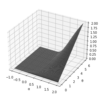
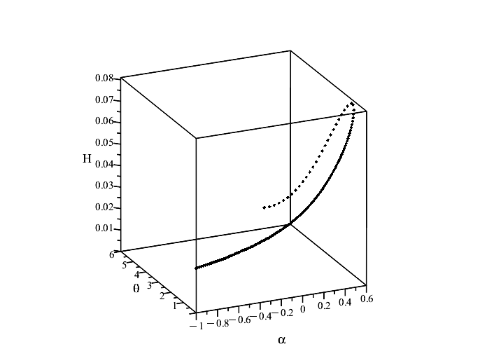
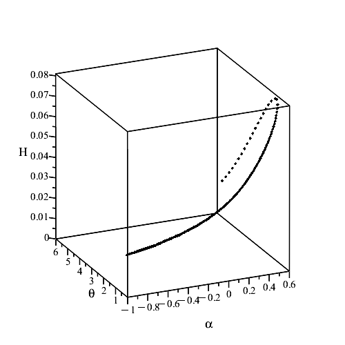
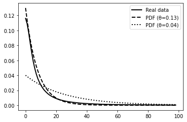
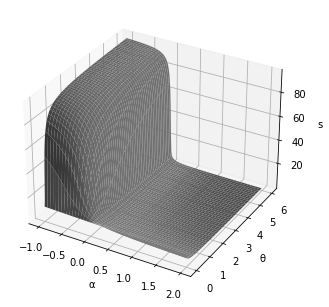
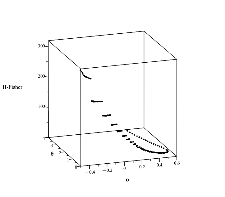
a­ b c d e f

Figure 1: First row: The H-C calculated using the histogram (d), critical points, and maximums. Second row: a histogram, central observations explained in P7-P9, and H-Fisher at the maximums.

We will now deal with second derivative of the two centralities at the critical points. Let us set $v(\theta,\alpha)=\sum_{i}\lambda_{i}x_{i}^{2}g_{\alpha}(x_{i}|\theta)-(\sum_{i}\lambda_{i}x_{i}g_{\alpha}(x_{i}|\theta))^{2}$, according to Eq . 19, the second derivatives at the critical point are given by:

$$\frac{\partial^{2}C_{\alpha}}{\partial\theta^{2}}=\left\{\begin{array}[]{l r }\frac{-2\alpha}{\theta^{2}}+\alpha^{2}\sum_{i}\lambda_{i}x_{i}^{2}g_{\alpha}(x_{i}|\theta)-(\alpha-1)^{2}\sum_{i}\lambda_{i}x_{i}^{2}g_{\alpha-1}(x_{i}|\theta)&\mbox{if $C=L$}\\ -\frac{1}{\theta^{2}}+\alpha v(\theta,\alpha)&\mbox{if $C=H$}\end{array}\right.$$ (26)

Note that, $v(\theta,\alpha)>0$. Indeed, let consider the positive function $\sum_{i}\lambda_{i}g_{\alpha}(x_{i}|\theta)(x_{i}-\sum_{j}\lambda_{j}x_{j}g_{\alpha}(x_{j}|\theta))^{2}$. It can be written as $\sum_{i}\lambda_{i}g_{\alpha}(x_{i}|\theta)x_{i}^{2}-2\sum_{i}\lambda_{i}g_{\alpha}(x_{i}|\theta)x_{i}\sum_{j}\lambda_{j}x_{j}g_{\alpha}(x_{j}|\theta)+(\sum_{j}\lambda_{j}x_{j}g_{\alpha}(x_{j}|\theta))^{2}$. Simplifying it gives $\sum_{i}\lambda_{i}x_{i}^{2}g_{\alpha}(x_{i}|\theta)-(\sum_{i}\lambda_{i}x_{i}g_{\alpha}(x_{i}|\theta))^{2}=v(\theta,\alpha)$. When it exists, the critical point of the H-C is a maximum if and only if $\alpha v(\theta,\alpha)<\frac{1}{\theta^{2}}$. More specifically, there is always a maximum when $\alpha\leq 0$ or when $\alpha v(\theta,\alpha)\in[0,\frac{1}{\theta^{2}}[$. Following the same reasoning for the case of L-C; the critical point is a maximum if $\sum_{i}\lambda_{i}x_{i}^{2}(\alpha^{2}g_{\alpha}(x_{i}|\theta)-(\alpha-1)^{2}g_{\alpha-1}(x_{i}|\theta))<\frac{2\alpha}{\theta^{2}}$. From this inequality, we deduce that if the left term is positive then $\alpha$ is positive and when $\alpha<0$ then the left term is negative. About the uncertainty, the H-Fisher information estimated at the maximums is plotted Fig. 1.f as function of $\alpha$ and $\theta$. The uncertainty is lower for higher $\alpha$. Another important question concerns the comparison of the C-estimator and the maximum likelihood estimator. We answer this question through an example in the case of H-Estimator. By using the histogram in Fig. 1.d, the best H-estimator according to the residuals $e_{H}$ in Eq. 20 when $\beta=2$ is $\theta=0.1300$ obtained at $\alpha=0.0800$ and leading to $e_{H}=0.0005$. For comparison purposes, the maximum likelihood estimator (i.e. $\alpha=0$) is $\theta=0.04$, which gives $e_{H}=0.0214$ for $\beta=2$. The estimated PDFs are plotted in Fig. 1.d.

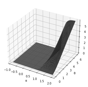
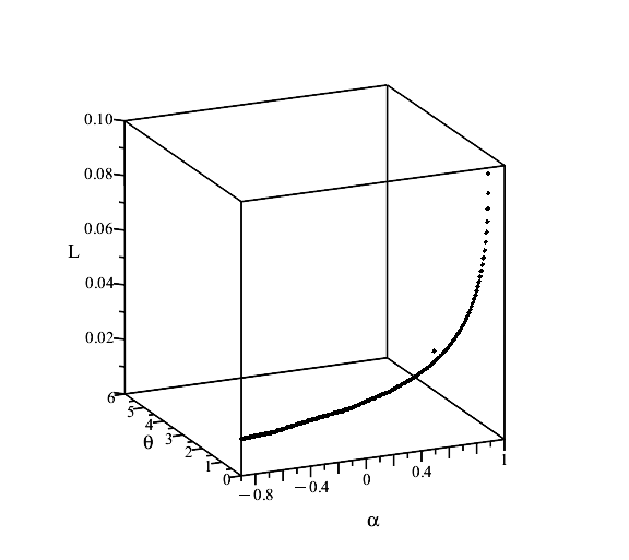
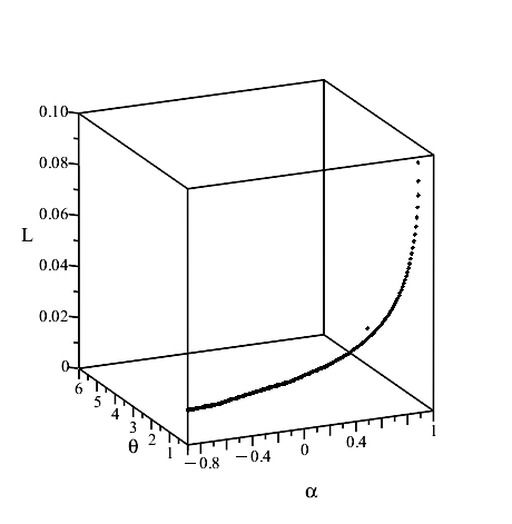
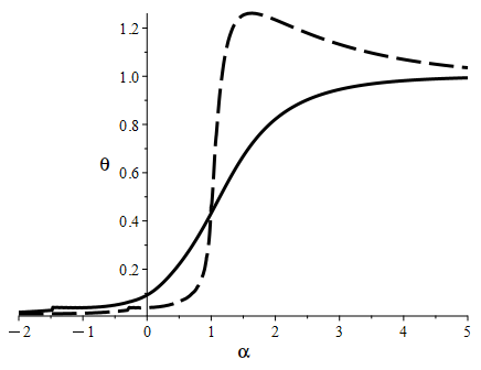
a b c h

Figure 2: First row: The L-C calculated using the histogram in 1.d., critical points, and maximums. Second row: the critical points $\theta$ of Hölder (solid) and Lehmer (dash) centralities as function of $\alpha$ drawn using the implicit function in Eq. 25.

We end this case study by presenting an example of histogram adjustment of the absolute values of the DCT coefficients. To do this, we examine the distribution of the parameter $\alpha$ leading to the best H-estimator according to $e_{H}()$ in Eq. 20. Fig. 3 presents the best H-estimators of 405 histograms of DCT coefficients extracted from gray-level images. In Fig. 3.a, an abscissa refers to a histogram and the corresponding ordinate is the value of the best H-estimator. For a histogram, the maximums of H-C are located and the one with the smallest $e_{H}()$ is chosen. The average $e_{H}()$ for the 405 histograms is 0.0008. The histogram of the variable $\alpha$ used to calculate the 405 best H-estimators is shown in Fig. 3.b. It can be observed that most of the values of $\alpha$ are not zero. Which indicates that, according to $e_{H}()$, maximum likelihood is not the best estimator.

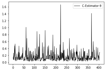
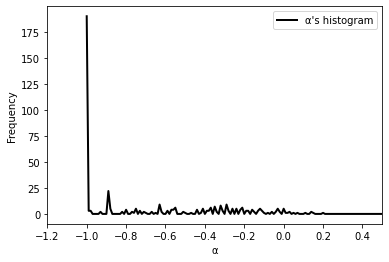
.a .b

Figure 3: Fitting of 405 histograms of DC coefficients. a) The H-estimator $\theta$ for each image. b) The histogram of the $\alpha$ selected according to the residual error.

References

- [1] V. Sundarapandian. Probability, statistics and queueing theory. PHI Learning Private Limited, New Delhi, 2009.
- [2] U. Berger, G. Baumgarten, J. Fiedler, F.-J. Lübken. A new description of probability density distributions of polar mesospheric clouds. Atmospheric Chemistry and Physics 19, pp. 4685-4702, 2019.
- [3] F. Kerouh, D. Ziou, and A. Serir. Histogram modelling-based no reference blur quality measure. Signal Processing: Image Communication 60, pp. 22-28, 2018
- [4] D. Ziou. Pythagorean Centrality for Data Selection. arXiv preprint arXiv:2301.10010, 2023.
- [5] D. Ziou. Using maximum weighted likelihood to derive Lehmer and Hölder mean families. arXiv preprint arXiv:2305.18366, 2023.
- [6] A. Charnes, E. L. Frome, and P. L. Yu. Equivalence of Generalized Least Squares and Maximum Likelihood Estimates in the Exponential Family. Journal of the American Statistical Association 71, pp. 169-171, 1976.
- [7] D. S. Pavlichin, J. Jiao, and T. Weissman. Profile Maximum Likelihood. Journal of Machine Learning Research 20, pp. 1-55, 2019.
- [8] B. Efron. Maximum likelihood and decision theory. The annals of statistics 10, pp. 340-356, 1982.
- [9] R. Ksantini, D. Ziou, B. Colin, and F. Dubeau. Weighted Pseudometric Discriminatory Power Improvement Using a Bayesian Logistic Regression Model Based on a Variational Method. IEEE TPAMI 30, pp. 253-266, 2008..
- [10] K. Giberta, M. Sànchez–Marrèb, and J. Izquierdo. A survey on pre-processing techniques: Relevant issues in the context of environmental data mining. AI Communications 29, pp. 627–663, 2016.
- [11] J. Aldrich. R. A. Fisher and the Making of Maximum Likelihood 1912 – 1922. Science 12, pp. 162-176, 1997.
- [12] R. A. Fisher. On the mathematical foundations of theoretical statistics. Philos. Trans. Roy. Soc. London Ser. A 222, pp. 309-368. 1922
- [13] NIST/SEMATECH e-Handbook of Statistical Methods. https://doi.org/10.18434/M32189, 2012.
- [14] D. Ziou, T. Hamri, and S. Boutemedjet. A hybrid probabilistic framework for content-based image retrieval with feature weighting. Pattern Recognition 42, pp. 1511-1519, 2009.
- [15] S. Boutemedjet and D. Ziou. Long-term relevance feedback and feature selection for adaptive content based image suggestion. Pattern Recognition 43, pp. 3925-3937, 2010.
- [16] E. F. Beckenbach. A Class of Mean Value Functions. The American Mathematical Monthly, pp. 1-6, 1950.
- [17] R. L. Berger and G. Casella. Deriving Generalized Means as Least Squares and Maximum Likelihood Estimates. The American Statistician, pp. 279-282, 1992.
- [18] C. Bishop. Pattern Recognition and Machine Learning. Springer-Verlag New York, 2006.
- [19] B. L. Burrows and R. F. Talbot. Which mean do you mean? Int. Journal of Mathematical Education in Science and Technology, pp. 275-284, 1986.
- [20] K. Cooray and M. M. A. Ananda. A Generalization of the Half-Normal Distribution with Applications to Lifetime Data. Communications in Statistics - Theory and Methods, pp. 1323-1337, 2008.
- [21] E. Díaz-Francés and F.J. Rubio. On the existence of a normal approximation to the distribution of the ratio of two independent normal random variables. Stat Papers 54, pp. 309–323, 2013.
- [22] F. Kerouh, D. Ziou, and A. Serir. Histogram modelling-based no reference blur quality measure. Signal Processing: Image Communication, pp. 22-28, 2017.
- [23] N. L. Johnson, S. Kotz, and N. Balakrishnan. Continuous Univariate Distributions, vol. 1. Wiley Series in Probability and Statistics, 2000.
- [24] H-T. Ku, M-C. Ku, and C-M. Zhang. Generalized power means and interpolating inequalities. Proc. of the American mathematical society 127, pp. 145-154, 1999.
- [25] J. Mićić, Z. Pavić, and J. Pečarić. The Inequalities for Quasiarithmetic Means. Abstract and Applied Analysis, 25 pages, 2012.
- [26] D. A. Pierce. Exponential Family: Overview. Chapter in John Wiley & Sons, 2014.
-
[27]
K. B. Stolarsky. Hölder Means, Lehmer Means, and . Journal of Mathemtica
l Analysis and Applications, pp. 810-818, 1996. - [28] V. Zografos, R. Lenz, M. Felsberg. The Weibull manifold in low-level image processing: An application to automatic image focusing. Image and Vision Computing, pp. 401-417, 2013.