Systematic Biases in Estimating the Properties of Black Holes
Due to Inaccurate Gravitational-Wave Models

Abstract

Gravitational-wave (GW) observations of binary black-hole (BBH) coalescences are expected to address outstanding questions in astrophysics, cosmology, and fundamental physics. Inference of BBH parameters relies on waveform models, and realizing the full discovery potential of upcoming LIGO-Virgo-KAGRA observing runs and new ground-based facilities (such as the Einstein Telescope and Cosmic Explorer) hinges on the accuracy of these waveform models. Using linear-signal approximation methods and Bayesian analysis, we start to assess our readiness for what lies ahead using two state-of-the-art quasi-circular, spin-precessing models: SEOBNRv5PHM and IMRPhenomXPHM. We find that systematic biases increase with the spin of the BH, with parameter biases being approximately 6 to 8 times likelier, if the primary-spin magnitude exceeds 0.5 compared to when it is less than 0.5. Additionally, we ascertain that current waveforms can accurately recover the distribution of masses in the LVK astrophysical population, but not spins. Upon exploring the broader parameter space of BHs, we find that systematic biases increase with detector-frame total mass, binary asymmetry, and spin-precession, with a majority of such binaries incurring parameter biases, extending up to redshifts $\sim 3$ in future detectors. Furthermore, we examine three “golden” events characterized by mass ratios of approximately 6 to 10, significant spin magnitudes ($0.6\mbox{--}0.9$), and high precession, evaluating how systematic biases may affect their scientific outcomes. Our findings reveal that current waveforms fail to enable the unbiased measurement of the Hubble-Lemaître parameter and sky localization from loud signals, even for current detectors. Moreover, highly asymmetric systems within the lower BH mass-gap exhibit biased measurements of the secondary-companion mass, which impacts the physics of both neutron stars and formation channels. Similarly, we deduce that the primary mass of massive binaries ($>60M_{\odot}$) will also be biased, affecting supernova physics. Future progress in analytical calculations and numerical-relativity simulations, crucial for calibrating the models, must target regions of the parameter space with significant biases to develop more accurate models. Only then can precision GW astronomy fulfill the promise it holds.

I Introduction

Almost a decade ago, the first observation of a gravitational wave (GW) from the coalescence of two black holes marked an important milestone in the history of GW astronomy [1]. Since then, the LIGO-Virgo-KAGRA (LVK) Collaboration [2, 3, 4] has detected more than 90 compact binary mergers [5, 6, 7], and independent research groups [8, 9, 10, 11, 12, 13] have discovered additional events. Thus, GWs have become a novel tool to explore the Universe. The observed signals have been used to measure the mass and spin distributions of BHs and neutron stars, their formation channels, and the co-evolution of their properties with that of the Universe [14, 15]. BNS mergers have improved the bounds on the nuclear equation of state and the maximum allowed mass of a NS [16, 17, 18]. The mass distributions have been employed to constrain the observed lower and predicted upper-mass gaps and other features in the mass spectrum. In conjunction with the electromagnetic (EM) counterparts observed for GW170817, or together with available galaxy catalogs, they have also been used to constrain the Hubble-Lemaître parameter ($H_{0}$) [19, 20]. GW measurements have also probed general relativity (GR) as the fundamental theory of gravity [21, 22, 23].

Improvements in the sensitivity of current GW detectors and proposed next-generation (XG) ground-based observatories like the Einstein Telescope (ET) and Cosmic Explorer (CE) [24, 25, 26], will significantly increase the observational volume, and with it the number of GW sources. For instance, a network of XG detectors will observe every stellar-origin BBH merger and most BNS mergers across the observable Universe [27]. A number of studies have explored in detail the extent to which various science objectives can be accomplished  [28, 29, 30, 31, 32, 27]. With $\mathcal{O}(100)$ observations by the LVK Collaboration, and $\mathcal{O}(10^{5})$ promised detections with XG detectors, meaningful inferences on the properties of the astrophysical distribution of BBHs will constrain more and more the underlying distribution of main sequence stars and their evolution. EM observations in our galaxy indicate that stellar-origin BHs have masses above $5\,\rm M_{\odot}$. However, these observations may be biased by properties that are unique to our galaxy. Similarly, the pair-instability supernova (PISN) process is expected to suppress BH formation in the mass range $\sim 50\mbox{--}120\,\rm M_{\odot}$ [33, 34]. Confident detections of BBHs in these mass ranges would pose challenges to stellar-evolution models, as well as, constrain the $\prescript{12}{}{C}(\alpha,\gamma)\prescript{16}{}{O}$ reaction rate that drives the PISN process [35]. Gravitational-wave astronomy can also determine the cosmological evolution of the Universe. In particular, by combining many GW signals, it will contribute to resolving the $H_{0}$ tension, and provide new constraints on structure formation. On the other hand, loud individual events carry a lot of information too. Individual “golden” BBHs can also resolve the Hubble-Lemaître tension [36]. Finally, precision tests of GR can be derived from high SNR observations [37, 38, 39, 40, 41, 42, 43]. All of these scientific objectives are vulnerable to false positives arising from waveform inaccuracies.

The source properties are estimated from the GWs via Bayesian inference using waveform models predicted by GR. Since there is no complete, closed-form analytic solution for the gravitational waveform of a compact-binary coalescence, various approximate and numerical methods have been developed to describe the GW signal faithfully. The effective-one-body (EOB) waveforms  [44, 45, 46, 47, 48, 49, 50, 51, 52, 53, 54, 55, 56, 57, 58] can combine and resum several perturbative results, such as post-Newtonian (PN), post-Minkowskian (PM) and gravitational self-force information for the conservative and dissipative dynamics, with physically motivated ansatze for the merger, and BH perturbation theory for the ringdown. They are made highly accurate through calibration to numerical relativity (NR) simulations [59, 60, 61]. Fast and accurate inspiral-merger-ringdown phenomenological (IMRPhenom) models [62, 63, 64, 65, 66, 67] are built fitting EOB, PN and NR waveforms. NR simulations give the most accurate representation of a GW signal although they are still limited by numerical truncation error [68, 69, 70], imperfect outer boundary conditions [71, 72, 73] and issues with GW extraction and extrapolation [74, 75]. Moreover, NR simulations are not available in the entire parameter space, and are limited in length due to their high computational cost. NR surrogate models (NRSur) [76, 77, 78, 79] are constructed by directly interpolating NR waveforms, where available.

Figure 1: The GW strains for a BBH system with parameters given in Table 1 (Binary 1) at the LIGO-Livingston detector of the O5 network. The black curve is the injected signal SEOBNRv5PHM, the green curve is the template IMRPhenomXPHM, evaluated for the injection parameters, and time shifted and global-phase rotated to maximize their overlap with the signal, while the brown curve is the template IMRPhenomXPHM evaluated at the maximum likelihood values obtained using a Bayesian analysis. The reference for the time axis, $t=0$, is taken to be the peak of the GW multipole $h_{22}$ of the signal.

Thanks to advancement in GW modeling since the discovery of GW150914 [80], waveform models have been sufficiently accurate to analyze most signals in the LVK GW Transient Catalogs (GWTC) [80, 81]. In Ref. [82], the authors used the absolute value of the difference between waveform models to quantify the accuracy of a given pair of models, finding that a few high signal-to-noise ratio (SNR) events in GWTC-3 and GWTC-2.1. fail their criterion. They also find that parameter estimation of such events show greater inconsistencies. A reanalysis of the GWTC-3 catalog by Ref. [83] finds that the NRSur7dq4 model recovers noticeably different parameters compared to LVK analyses using IMRPhenomXPHM and SEOBNRv4PHM waveform models for $\sim 20\%$ of the events where NRSur7dq4 model can be used . A hypermodel approach to identify waveform systematics has also been carried out on the 13 heaviest GW events from the GWTC-3 catalog. In this approach, waveform models are treated as parameters and directly sampled over, yielding a direct probability for each waveform model. The authors do not find any waveform model to be preferred except for 3 events which are marred by data quality issues [84]. Recently, there have also been efforts to marginalize over waveform modeling uncertainties [85, 86]. Other studies have found that even relatively low SNR events could be affected by systematic biases if they lie in a region of the parameter space where calibration with NR is sparse. This would include binaries that are asymmetric, eccentric, have large spin magnitudes, and/or have precessing orbits [51, 82].

With increasing detector sensitivity and number of detections, the median SNR of the observed population of binaries, as well as the likelihood of detecting a binary from a region of the parameter space where waveform inaccuracies are greater, will increase. While statistical uncertainties decrease with increasing SNR, systematic biases are independent of the signal power. Several studies have explored the validity of waveform models for the parameter estimation of quasi-circular binary black hole (BBH) mergers in upgraded and XG detectors, mainly focusing on the biases for individual events [87, 81, 82, 223], with Ref. [81] also showing the inferred distribution of the primary mass to be biased. While the negligence of subdominant modes can significantly bias the parameter estimation of individual events [88, 89], a recent study indicated that such biases do not affect the inference of the LVK-like astrophysical distribution of BBHs [90]. Other studies have focused on waveform systematics in the presence of eccentricity [91, 92], matter effects and spin-precession [93, 94, 95, 96, 97]. Recent studies have also explored the effect of truncation errors in NR simulations employing finite differencing methods and concluded that current simulations are not accurate enough for highly asymmetric binaries and binaries whose orbits are inclined with respect to the line of sight [98, 99]. However, state-of-the-art waveform models, such as SEOBNRv5PHM and IMRPhenomXPHM, are calibrated to the Simulating-eXtreme-Spacetimes (SXS) Collaboration waveforms, which employ spectral methods and the effect of truncation errors on these waveforms have not been explored systematically. An indistinguishability criterion [100] has also been used as an easy-to-compute metric to determine accuracy requirements of waveforms [101, 81]. However, this measure has been found to be very conservative. Reference [102] proposes a correction to it to improve the reliability of the measure.

We illustrate the effect of waveform mismodelling in Fig. 1, using a BBH with parameters given in Table 1 . We show the multipolar, spin-precessing GW strains in the LIGO-Livingston detector from the SEOBNRv5PHM waveform model [51] as signal (black curve) and the IMRPhenomXPHM waveform model [65] as template (brown and green curves). For the green curve, we fix the polarization angle and time at coalescence, by maximizing its overlap against the SEOBNRv5PHM signal. We employ the LIGO-Virgo detectors assuming the sensitivity of the upcoming fifth observing (O5) run. If the green GW strain faithfully represented the signal (black), they would perfectly match throughout the coalescence. However, this is not the case, the amplitude modulations are different during the long inspiral, and in particular during the late inspiral, merger and ringdown. Furthermore, while the signal and the template phases match during the early inspiral, there is significant dephasing near the late inspiral, merger and ringdown. In Fig. 1, we also show the IMRPhenomXPHM template (brown curve) evaluated at the maximum-likelihood parameters (obtained through a Bayesian analysis). It has a much better match to the SEOBNRv5PHM signal even during the late inspiral, merger and ringdown. This best match is obtained at the expense of introducing a bias in the parameters, notably the total mass, mass ratio, and the spin-precession parameter are biased by $\sim 3\%$, $\sim 6\%$ and $\sim 13\%$, respectively. The brown curve also has an associated brown band representing the measurement errors at 90% credible interval in the GW parameters, but it is barely visible to the naked eye, illustrating that this uncertainty, which represents the estimated statistical uncertainty from instrumental noise is much smaller than the waveform difference between the signal and the template evaluated at the best-fit parameters. As previously stated, this inconsistency manifests itself as biased parameter estimation, which could affect the various science objectives.

In this work, we start to quantify the systematic biases that can be expected in future observing runs with current facilities and XG detectors using the SEOBNRv5PHM and IMRPhenomXPHM waveform models, which are employed for parameter-estimation studies of BBHs by the LVK Collaboration. Both models are valid for quasi-circular binaries and incorporate subdominant spherical harmonics and spin-precession effects. While it would be ideal to quantify the biases of each of these models against the true GR signal, it is infeasible to do it everywhere in the parameter space since NR waveforms are not available. We leave to a future study the use of NR waveforms as synthetic signals where available. Throughout this paper, we instead generate GW signals using SEOBNRv5PHM, considering these to represent the true signal, and analyze them using IMRPhenomXPHM. However, there is a drawback to this approach. If both the waveform models deviate in a similar way from the true GR signal, the present analysis would predict small biases even when the true bias is large. This is especially true since the two waveform models are not completely independent. IMRPhenomXPHM uses the SEOBNR waveforms (although from a previous version, i.e., SEOBNRv4) for calibration in parts of the parameter space where there is a dearth of NR simulations. This is precisely the regions where systematic biases are expected to be more common. In this sense, our analysis is a conservative assessment of the prevalence of systematic biases.

To quantify the systematics of the aforementioned waveform models in a wide range of applications, we utilize Bayesian analysis as well as the linear-signal approximation (LSA). The former is the most reliable tool to obtain the posterior distribution for a GW signal, but computationally expensive. The latter allows for computational efficiency, but approximate the predictions for the posterior properties, including systematic biases, and should become a good approximation only at large SNR. We use the LSA to study biases for BBH populations, and a wider parameter space, which is not feasible with conventional Bayesian methods. We consider three detector networks comprising of the current LIGO-Virgo network at design sensitivity (O5), a planned network where the current LIGO detectors are upgraded to improved sensitivity (A#), and a XG network comprising of two CE and an ET. The BBH populations we consider follow the LVK-like distributions where the binary masses are distributed as determined by LVK while the spins are assumed to be isotropically oriented and distributed uniformly in magnitude. We do this to allow for a wider range of spins. The binaries extend up to a redshift of 3 following the Madau-Dickinson star formation rate (SFR) [103]. Following this, we embark on a parameter-exploration study where we consider large redshifted total masses of $200\rm\,M_{\odot}$, asymmetric systems with inverse mass ratios going up to 30, and highly spin-precessing systems. We study these as-yet unobserved regions of the parameter space in anticipation of future observations. We also consider three distinct prototypes of BBH mergers, which hold great potential for various science objectives, but are non-trivial to model due to precession or large mass ratio. The details of these three “golden” binary systems can be found in Table 1.

The paper is organized as follows. In Sec. II, we introduce the main characteristics of the GW signal and its parameters, the waveform models that we use, and the detector networks in which signals are simulated. In Sec. III, we describe our methodology comprising of Bayesian analysis and LSA. We point out the importance of having consistent parameter definitions across waveform models, and its impact on the systematic bias, where we show a comparison of a Bayesian analysis with the estimates from LSA. We also discuss the limitations of the LSA for parameter estimation (notably the Fisher information matrix) and biases. The study of systematic biases in the LVK-like BBH population and a hierarchical Bayesian inference on parameter distributions, reweighted to the LVK population, is reported in Sec. IV. A much broader study across the binary parameter space with particular focus on massive, highly asymmetric and spin-precessing binaries is reported in Sec. V. A ramification on the different science applications for GWs can be found in Sec. VI where we study selected GW events or “golden” binaries. The discussion and conclusion can be found in Sec. VII. In Appendix A, we illustrate the effect of nonuniform-parameter definitions across waveform models on the estimates of the systematic bias through a toy model. In Appendix B, we discuss the effect of different harmonics of the EOB model starting at different frequencies. In Appendix C, we discuss the effect of the starting frequency of the analysis on parameter estimation and systematic biases. In Appendix D, we provide a complimentary plot to Fig. 6 by reporting the dependence of ratio of systematic bias to statistical error as a function of the SNR. In Appendix E, we show the effect of the SNR threshold on the distribution of the population parameters. In Appendix F, we report the bias horizon for the $\chi_{1}$ parameter of the exploratory binaries of Sec. V.

II Gravitational-wave parameters, models and detectors

II.1 Gravitational-wave parameters

We are interested in estimating the properties of quasi-circular, spin-precessing BBHs observed with current and future ground-based detector networks. The GW strain emitted by such binaries is characterized by 15 parameters. The parameters intrinsic to the source are the component masses, $m_{i}$  and the dimensionless spin vectors, $\bm{\chi}_{i}=\bm{S}_{i}/m_{i}^{2}$ $(i=1,2)$. The position of the binary is described by its luminosity distance, $D_{L}$, and the coordinates on the plane of the sky, $(\alpha,\delta)$. The orientation of the binary is described by the polar angle, $\iota$, and the azimuthal angle, $\varphi$, to the observer in the source frame [104] at the reference frequency, $f_{\rm ref}$, which we set to $f_{\rm ref}=20\rm\,Hz$ throughout this paper. Finally, the relative contribution of the two gravitational polarizations, $h_{+}(t)$ and $h_{\times}(t)$, is described by the polarization angle, $\psi$, while the reference for the time is given by the coalescence time, $t_{c}$. With these definitions, the GW strain can be expressed as

$$\begin{split}h(t)=&h_{+}(t;m_{z,i},\bm{\chi}_{1,2},D_{L},\iota,\varphi,t_{c})F_{+}(\alpha,\delta,\psi)\\ &+h_{\times}(t;m_{z,i},\bm{\chi}_{1,2},D_{L},\iota,\varphi,t_{c})F_{\times}(\alpha,\delta,\psi)\,,\end{split}$$ (1)

where $F_{+,\times}(\alpha,\delta,\psi)$ are the antenna pattern functions [105, 106]. The detector- and source-frame masses, $m_{i}^{z}$ and $m_{i}$, respectively, are related by $m_{z,i}=m_{i}(1+z)$ with $z$ being the redshift of the source. A superscript on any mass parameter indicates that it is detector frame while its absence indicates it is source frame. The parameters $D_{L}$ and $z$ are related for a given cosmological model, which we take to be the one from Planck18 [107]. The two GW polarizations can be decomposed in the basis of $-2$ spin-weighted spherical harmonics, $\prescript{}{-2}{Y}_{lm}$, as

$$h_{+}(t)-ih_{\times}(t)=\sum_{l=2}^{\infty}\sum_{m=-l}^{+l}\prescript{}{-2}{Y}_{lm}(\iota,\varphi)h_{lm}(t)$$ (2)

where $h_{lm}(t)$ are the GW multipoles and $\varphi=\pi/2-\phi_{\rm ref}$.

It is often helpful to express the GW signal in terms of parameters that are combinations of the component masses and spins, either because they appear in such combinations in PN expressions or because they are conserved up to certain PN orders. In particular, the chirp mass, $\mathcal{M}_{c}$, and the symmetric mass ratio, $\nu$, are defined by $\mathcal{M}_{c}=(m_{1}m_{2})^{3/5}/M^{1/5}$ and $\nu=(m_{1}m_{2})/M^{2}$, respectively, where $M=m_{1}+m_{2}$ is the total mass. The effective spin, $\chi_{\rm eff}$, and spin-precession, $\chi_{\rm p}$, parameters are given by

$$\chi_{\rm eff} =\frac{m_{1}\chi_{1z}+m_{2}\chi_{2z}}{m_{1}+m_{2}}\,,$$ (3a)

$$\chi_{\rm p} =\frac{1}{B_{1}m_{1}^{2}}\max{(B_{1}m_{1}^{2}\chi_{1,\perp},B_{2}m_{2}^{2}\chi_{2,\perp})}\,,$$ (3b)

where $B_{1,2}=2+3\,m_{2,1}/m_{1,2}$, and $\chi_{i\perp}$ and $\chi_{iz}$ are the magnitudes of the projection of $\bm{\chi}_{i}$ on to the orbital plane and perpendicular to it, respectively. While alternative definitions of $\chi_{\rm p}$ have been proposed [108, 109], the GW–Bayesian-analysis package Bilby that we use to analyze simulated signals uses Eq. (3b).

When transforming to a spherical coordinate system with the $z$-axis perpendicular to the instantaneous orbital angular momentum, the tilts of the two spin vectors with respect to the $z$-axis, $\theta_{i}$, are given by

$$\cos\theta_{i}=\frac{\chi_{iz}}{\chi_{i}}\,,$$ (4)

where $\chi_{i}\equiv|\bm{\chi}_{i}|$ are the magnitudes of the dimensionless spin vectors. The relative angle between them in the orbital plane is parameterized by $\phi_{12}=\phi_{1}-\phi_{2}$ where $\phi_{1,2}$ are the azimuthal angles of the two spin vectors in the spherical coordinates. Finally, the direction of the total angular momentum, $\bm{J}$, in the plane perpendicular to the orbital angular momentum, $\bm{L}$, at some reference time is given by the parameter $\phi_{\rm JL}$. Since $\bm{J}=\bm{L}+\bm{S}_{1}+\bm{S}_{2}$, $\phi_{\rm JL}$ also defines the direction of the total spin vector in the orbital plane. The total angular momentum also defines the angle, $\theta_{\rm JN}$, which gives the orientation of the total angular momentum vector relative to the line-of-sight, $\bm{N}$, of the observer. The angle $\theta_{\rm JN}$ can be expressed in terms of the inclination angle, $\iota$, at the reference frequency, $f_{\rm ref}$, e.g., through Eq. (C9) of Pratten et al. [65]. In summary, the waveform depends on the following 15 parameters:

$$\bm{\vartheta}=\{\mathcal{M}_{c},\nu,\chi_{i},\cos\theta_{i},\phi_{\text{JL}},\phi_{12},\alpha,\delta,D_{\text{L}},t_{\text{c}},\theta_{\text{JN}},\psi,\phi_{\rm ref}\}.$$ (5)

In the following, we will use a bold-face variable, like $\bm{\vartheta}$, to describe a set of parameters and regular-face variable, like $\vartheta$, to describe a particular parameter in the set.

II.2 Waveform models

We consider two state-of-the-art, quasi-circular spin-precessing waveform models incorporating subdominant spherical harmonics — SEOBNRv5PHM and IMRPhenomXPHM. The GW modes $(l,m)\neq(2,2)$ are important both for detection [110, 111, 112], where their non-inclusion leads to a loss of signal power for asymmetric binaries and inclined orbits, and parameter estimation, where these modes can break degeneracies between various parameters and improve the measurement accuracy [88, 89, 113, 114].

The SEOBNRv5PHM waveforms contain the spherical harmonics $(l,|m|)=(2,2),(2,1),(3,3),(3,2)$, and $(4,4),(4,3),(5,5)$ in the coprecessing frame. However, in this paper we do not include the $(l,m)=(5,5)$ mode. The IMRPhenomXPHM waveforms include the $(l,|m|)=(2,2),(2,1),(3,3),(3,2),(4,4)$ modes in the coprecessing frame . Both waveform models can be used for a wide range of mass ratios, as well as BH-spin magnitudes up to the maximal values. However, only the aligned-spin sectors of both waveform models were calibrated to NR simulations, and their accuracy has been assessed only in regions of parameter space where NR is available.

In this work, we consider a signal generated using the SEOBNRv5PHM model to be the true GW signal and analyze it using IMRPhenomXPHM as the template model. For the Bayesian analyses of this paper, this is done because IMRPhenomXPHM is quicker to evaluate due to it being a frequency-domain model while SEOBNRv5PHM is a time-domain model and it is slower. Furthermore, the computational efficiency of IMRPhenomXPHM can be improved by utilizing the multibanding approach [116] while no such analogous methods exist for time-domain models. For the Fisher–information-matrix analysis discussed later, we find instabilities in the numerical derivatives of the SEOBNRv5PHM waveform with respect to the GW parameters, for some regions of the parameter space, and hence restrict ourselves to computing derivatives of the IMRPhenomXPHM model. We expect to address this issue in the future.

II.3 Detector networks

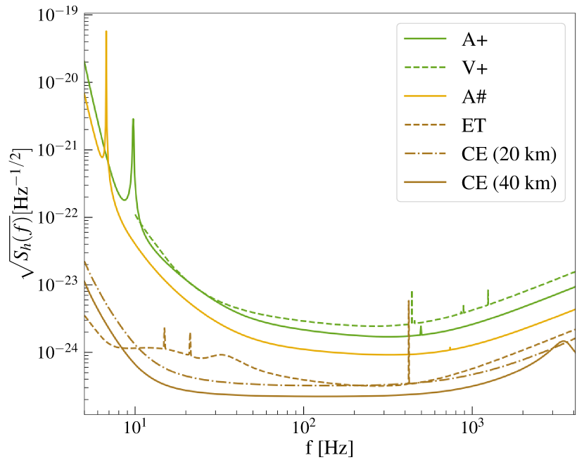
Figure 2: The amplitude–spectral-density curves of the various detectors used in this paper (see footnote 5). The curves labeled by A+ and V+ denote the design sensitivity of the LIGO and Virgo detectors, respectively, which form part of the network of the fifth observing run (O5), while A# refers to the LIGO detectors at upgraded sensitivity. The next-generation observatories are the ET and CE with the baseline network for the latter consisting of a 20 km and a 40 km detector.

The current detectors are expected to achieve design sensitivity in the next few years, during the fifth observing (O5) run, and continue operating till the end of the decade [117]. It is anticipated that the detectors would undergo major upgrades thereafter and operate until next-generation detectors come online or even in tandem with them. Since plans for future detector networks have not yet been finalized, a number of studies have explored the capabilities of different combinations of detector configurations to understand what the optimal design is for various science goals [27, 29, 30, 118, 28]. In this work, three GW detector networks, consisting of the current detectors at design and upgraded sensitivity, and proposed future detectors, are considered to emulate a highly probable observing scenario for the coming decades . These are enumerated below:

• O5 network: This is comprised of the advanced LIGO detectors located at Hanford and Livingston, and the advanced Virgo detector operating at design sensitivities, A+ and V+, respectively.

• A# network: In this configuration, the LIGO detectors operate at upgraded A# sensitivity while the Virgo detector continues to operate at design sensitivity, V+.

• XG network: This comprises of three proposed XG observatories consisting of the baseline 40 km and 20 km CE in the United States, and an ET in Europe.

The power spectral density (PSD) of the individual detectors are shown in Fig. 2.

III Statistical Methods

This section describes the data-analysis methods used in this paper. In Sec. III.1 we start by describing the Bayesian framework for analyzing GW signals and lay out the different choices of priors and frequency bands used for the different networks. Thereafter, in Sec. III.2, we introduce the LSA for the likelihood, and recount the Fisher information matrix (FIM) [105] method for estimating measurement errors. Following that, in Sec. III.3, we elucidate the computation of biases (or systematic errors) under the LSA [100, 119], and emphasize the importance of minimizing the mismatch between (i.e., aligning) the signal and template for reliable estimates of the bias. As an example, we compare the posterior distributions for a chosen binary system, as obtained from a full Bayesian analysis with the estimates from the LSA. Specifically, we point out the differences if the bias is computed without aligning the two waveforms. Finally, in Sec. III.4 we discuss the hierarchical Bayesian method, which we employ to understand the impact of biases on the inference of the properties of the BBH population.

III.1 Bayesian analysis

The posterior probability distribution on the parameters of the waveform model, $\bm{\vartheta}$, given the observational data $d$, and the hypothesis (model description) $\mathcal{H}$, is obtained using Bayes’ theorem,

$$p(\bm{\vartheta}|d,\mathcal{H})=\frac{p(d|\bm{\vartheta},\mathcal{H})\,p(\bm{\vartheta}|\mathcal{H})}{p(d|\mathcal{H})}\,,$$ (6)

where $p(\bm{\vartheta}|\mathcal{H})$ is the prior probability distribution, $p(d|\bm{\vartheta},\mathcal{H})$ is the likelihood function, and $p(d|\mathcal{H})$ is the evidence of the hypothesis $\mathcal{H}$. If one is interested solely in parameter estimation, and not in model selection, the latter serves as a normalization constant, and can be discarded.

For a detector with stationary, Gaussian noise, the likelihood function for the data given the parameters $\bm{\vartheta}$ is defined as

$$\ln p(d|\bm{\vartheta})=\left<d-h(\bm{\vartheta})|d-h(\bm{\vartheta})\right>\,,$$ (7)

where we define the noise-weighted inner product as

$$\left<h_{1}|h_{2}\right>=4\Re\left[\int_{f_{\text{low}}}^{f_{\text{high}}}\frac{h_{1}(f)\times h_{2}^{*}(f)}{S_{h}(f)}df\right]$$ (8)

with $S_{h}(f)$ being the noise PSD, and $f_{\text{low}}$ and $f_{\text{high}}$ are the minimum and maximum frequency in the detectors’ bandwidth. This inner product also defines the optimal, matched-filtering SNR in a detector, $\rho_{n}$, by

$$\rho_{n}^{2}=\left<h(\bm{\vartheta})|h(\bm{\vartheta})\right>.$$ (9)

The total SNR is $\rho^{2}=\sum_{n=1}^{N}\rho_{n}^{2}$, where $N$ is the number of detectors in the network. We note that all our injections are noiseless which corresponds to averaging over multiple noise realizations.

While the current detectors’ sensitivity is limited to a minimum frequency of 20 Hz, at design sensitivity and with further upgrades, they are expected to reach a low-frequency sensitivity of 10 Hz. Meanwhile, XG observatories are aiming to further this improvement to 5 Hz. Therefore, the minimum frequency for the O5 and A# networks are assumed to be $f_{\text{low}}=10\,\rm Hz$, while for XG detectors, it is taken as $f_{\text{low}}=5\,\rm Hz$. On the other hand, the maximum frequency is kept the same for all three networks at $f_{\text{high}}=1024\,\rm Hz$. This does not limit the analysis whatsoever since all the BBH systems considered in Sec. VI merge at much lower frequencies.

As we mentioned earlier, the signal is generated using the SEOBNRv5PHM model with the same starting frequency as the analysis — $f_{\text{low}}=10\,\rm Hz$ for O5 and A#; $f_{\text{low}}=5\,\rm Hz$ for XG. Since SEOBNRv5PHM is a time-domain waveform model, this $f_{\text{low}}$ refers to the starting frequency of the $(l,m)=(2,2)$ mode. Subdominant harmonics with $m^{\prime}\neq 2$ start at higher frequencies given by $f_{lo}^{m^{\prime}}={m^{\prime}}f_{lo}/2$. For instance, in O5 and A# networks, the $m^{\prime}=3$ modes start at 15 Hz while the $m^{\prime}=4$ modes start at 20 Hz. In Appendix B, we show that this choice does not affect our results. This is because of the minimal additional information contained in the missing frequencies compared to the rest of the signal.

To simulate and analyze the GW signals in Sec. VI, we use the publicly available Bilby package [120, 121], which incorporates the nested sampler dynesty [122], interfaced through the Bilby-pipe wrapper. Initially, a 14-dimensional GW parameter space is sampled using the dynesty sampler with a distance-marginalized likelihood. The full posterior probabilities are then reconstructed using semi-analytic methods [123, 124].

All the detectors used in this study have an L-shaped interferometer configuration except the ET, which is proposed to have a triangular configuration. However, the Bilby-pipe wrapper is limited to L-shaped interferometer configurations. Consequently, the ET telescope is assumed to be L-shaped in Sec. VI. Our conclusions remain unaffected as the interferometer’s shape has no significant impact on the science cases discussed here [30].

We make standard choices for the priors for all the parameters [125]. The priors for the component masses are taken to be uniform, and the spins are assumed to be isotropic in direction and uniform in magnitude. For the distance we choose the prior $\propto d_{L}^{2}$, corresponding to a uniform in comoving volume distribution at low redshift. We assume that the binary’s position in the sky and the inclination of its orbit in the coprecessing frame are random. Therefore, we assign uniform priors on $\alpha$, $\cos\delta$, and $\cos\theta_{\rm JN}$ across their domains. The other extrinsic parameters, namely, the polarization angle, coalescence time, and coalescence phase are also taken to be uniform in their respective ranges.

III.2 Linear-signal approximation for measurement errors, systematic biases and alignment

Measurement errors

The evaluation of the posterior probability distribution, as described in the previous section, is computationally expensive. This makes the estimation of the measurement accuracies and systematic biases for large number of sources computationally prohibitive using the Bayesian method. An inexpensive approximate method is the LSA, which we now briefly introduce.

To estimate the parameter-estimation errors, the waveform model is expanded to linear order in the parameters around the maximum likelihood (best-fit) values, $\bm{\vartheta}_{\text{bf}}$. This results in a Gaussian likelihood distribution whose covariance, $C_{ij}$, is given by the inverse of the FIM, $C_{ij}=\Gamma_{ij}^{-1}$, which takes the form [105, 119],

$$\Gamma_{ij}\equiv\left<\frac{\partial h}{\partial\bm{\vartheta}^{i}}\middle|\frac{\partial h}{\partial\bm{\vartheta}^{j}}\right>\bigg{|}_{\bm{\vartheta}=\bm{\vartheta}_{\text{bf}}}.$$ (10)

The marginalized one-dimensional errors are then given by the diagonal elements, $\Delta\bm{\vartheta}^{i}=\sqrt{C_{ii}}$ . The approximation holds for large SNR.

We use the publicly available package GWBENCH [126] to calculate the measurement errors. GWBENCH is an easy-to-use FIM analysis tool for ground-based detectors that implements finite difference derivatives to estimate the approximate measurement errors. Other recent FIM analysis codes for compact-binary coalescences are GWFAST [32] and GWFish [127]. The waveform models are internally referenced from the LALSuite [128] libraries. While the IMRPhenomXPHM model is directly present in LALSuite, the SEOBNRv5PHM model is interfaced through the pySEOBNR package [129] within LALSuite. For IMRPhenomXPHM, the default model in LALSuite implements a multibanding approach [116] for faster waveform computation. However, we turn this off in our FIM analysis because we found that the output of the last frequency bin has some randomness associated to it. This is harmless in a Monte Carlo sampling of the likelihood since the amplitude in that frequency bin is subdominant and does not contribute to the integral of Eq. (7). However, a FIM analysis involves taking waveform derivatives with respect to binary parameters and the randomness manifests as a delta-function which dominates the integral in Eq. (10).

Systematic biases

A further assumption in the FIM formalism is that there are no mismodeling errors, that is, the signal is accurately represented by the model waveform and errors are only due to a measurement process using detectors with finite sensitivity. In reality, we do not know the true GW waveform and use various approximate models to faithfully represent the true signal. As such, there is a source of error arising from a difference between the signal and the waveform model used to represent the signal (template). As a result, the parameters that maximize the likelihood are biased from the true parameters of the GW signal by $\delta\bm{\vartheta}^{i}$. This mismodeling error, henceforth called bias $\delta\bm{\vartheta}^{i}$, is given by [100, 119],

$$\delta\bm{\vartheta}^{i}=C^{ij}\,\left<\partial_{j}h|\delta h\right>\big{|}_{\bm{\vartheta}=\bm{\vartheta}_{\text{bf}}},$$ (11)

at the leading order, where $\delta h=h_{\text{s}}-h$ with $h_{\text{s}}$ being the true signal. In practice, the true signal is not known, so this formula can only be used if the true signal is replaced by some fiducial reference model, here taken to be SEOBNRv5PHM.

Waveform alignment

We now discuss a few subtleties in the use and applicability of Eq. (11) for the estimation of biases. Note that the bias is directly proportional to the waveform difference, $\delta h$. In part due to different conventions for some extrinsic parameters, $\delta h$ can be artificially large when evaluated at the same value of all parameters, but can be significantly reduced by changing the values of certain extrinsic parameters, such as the global phase and time shift, while keeping the intrinsic parameters fixed. In Appendix A we describe a toy model that illustrates how a simple time shift can cause biases in physical parameters to become large. Since Eq. (11) is derived under the LSA, large waveform differences stretch the formula beyond its domain of validity resulting in unreliable estimates. However, large uncertainties in the extrinsic parameters are typically not problematic for scientific applications of GW observations, so if, by changing only a subset of the extrinsic parameters, we can bring the waveform difference back into the range of validity of the LSA, this should be done to improve the accuracy of the inferred results.

Waveform-accuracy studies in the literature that use $\delta h$ as a metric to quantify waveform differences, and estimate expected biases, have typically followed this approach and minimized $\delta h$ over the extrinsic parameters [130, 82] (alignment). However, to the best of our knowledge, many studies employing Eq. (11) to estimate the bias either neglect this aspect and naively use the difference between waveform models to estimate the systematic bias, or at least do not discuss it. The incorrect use leads to unreasonably large estimated biases, particularly for the luminosity distance. Therefore, we describe here how we implement the alignment in the bias formula.

Using Eq. (8), we define the unfaithfulness or mismatch between two waveforms $h_{1}$ and $h_{2}$ as

$$\mathcal{M}=\min_{\bm{\lambda}}\left\{1-\frac{\left<h_{1}|h_{2}\right>}{\sqrt{\left<h_{1}|h_{1}\right>\left<h_{2}|h_{2}\right>}}\right\}$$ (12)

where the minimization is done on a subset of the binary’s parameters that we denote $\bm{\lambda}$. For nonprecessing waveform models employing only the dominant quadrupolar mode, $\bm{\lambda}=\{\psi,t_{c}\}$. In this case, $\psi$ is degenerate with $\phi_{\rm ref}$, so we need to consider only one of them. On the other hand, since we are considering spin-precessing waveform models, $\bm{\lambda}=\{\psi,t_{c},\phi_{\rm ref},\phi_{\rm JL}\}$ where $\phi_{\rm JL}$ is a rotation of the in-plane spin angles. For spin-precessing waveform models, some studies have chosen to minimize the mismatch over the reference frequency instead of in-plane spin rotations [131, 132]. However, in this study, we choose to optimize the mismatch by rotating the in-plane spin components [65, 51], thus keeping the reference frequency fixed at $f_{\rm ref}=20\rm\,Hz$.

Starting with the set of parameters $\bm{\vartheta}$, we find the parameters $\overline{\bm{\lambda}}$ that minimizes $\mathcal{M}$ in Eq. (12) for the detector network being considered. The minimization over the polarization angle $\psi$ is done analytically, while the coalescence time $t_{c}$ is optimized by convolving the two waveforms utilizing the convolution theorem [106, 133, 134]. The reference phase $\phi_{\rm ref}$ and in-plane spin rotations $\phi_{\rm JL}$ are optimized numerically by using standard optimization algorithms. Having found the parameters that minimize Eq. (12), $\overline{\bm{\lambda}}$, we have a new set of parameters $\overline{\bm{\vartheta}}_{\text{bf}}$, where the parameters $\bm{\lambda}=\{\psi,t_{c},\phi_{\rm ref},\phi_{\rm JL}\}$ have been replaced by the values obtained through Eq. (12). This is the set of parameters that we use to compute the FIM, as well as, the $\delta h$ in Eq. (11). Therefore, the alignment procedure modifies Eq. (11) to

$$\delta\bm{\vartheta}^{i}=C^{ij}(\overline{\bm{\vartheta}}_{\text{bf}})\,\left<\partial_{j}h(\overline{\bm{\vartheta}}_{\text{bf}})|h_{\text{s}}(\bm{\vartheta})-h(\overline{\bm{\vartheta}}_{\text{bf}})\right>\,.$$ (13)

If the parameters $\bm{\lambda}$ are uncorrelated to the other binary parameters, the bias formula Eq. (11) should give $\delta\bm{\lambda}=0$. However, in general, that is not the case and, therefore, $\delta\bm{\lambda}\neq 0$. Thus the total bias for $\bm{\lambda}$ is $\Delta\bm{\lambda}=\delta\bm{\lambda}+\left(\bm{\lambda}_{s}-\overline{\bm{\lambda}}\right)$ where $\bm{\lambda}_{s}-\overline{\bm{\lambda}}$ is the difference between the parameters $\bm{\lambda}$ of the fiducial signal and those obtained after the optimization procedure.

Note that we chose to modify the template in Eq. (11) following the optimization procedure Eq. (12). Under the LSA, we are free to modify the signal evaluating the template at the fiducial parameters. However, we notice a slightly better agreement of the bias with full Bayesian results when modifying the template. This is because the Bayesian analyses are performed using the fiducial parameters as the values of the synthetic-injected signal, and we find the systematic bias to be more sensitive to small changes in the injected values compared to the measurement errors.

Lastly, we note that $\mathcal{M}$ could already be close to the minimum for certain pairs of waveform models at a given set of parameters out of the box. In such cases, the optimization procedure will have minimal effect on the total bias and one could simply use the bias formula as it is. However, the total bias $\Delta\bm{\lambda}$ would be the same regardless of whether one chooses to do the initial optimization or not even though the output of the bias formula will not be. For the same reason, the net bias does not depend sensitively on the precision of the optimization routine as the bias formula compensates for it. Therefore, it is more prudent to compare the net biases rather than the optimized values following the initial minimization. We have verified our minimization procedure using a brute-force 4D minimization algorithm and find that while $\overline{\bm{\lambda}}$ is slightly different between the two minimization routines, $\Delta\bm{\lambda}$ remains the same.

In the following, we calculate the systematic biases with and without the optimization procedure outlined above. We compare these estimates with the full Bayesian-analysis results for a subset of the parameters, and find agreement with the Bayesian analysis when using the optimization procedure Eq. (12).

III.3 Comparing Bayesian and linear-signal approximation analyses

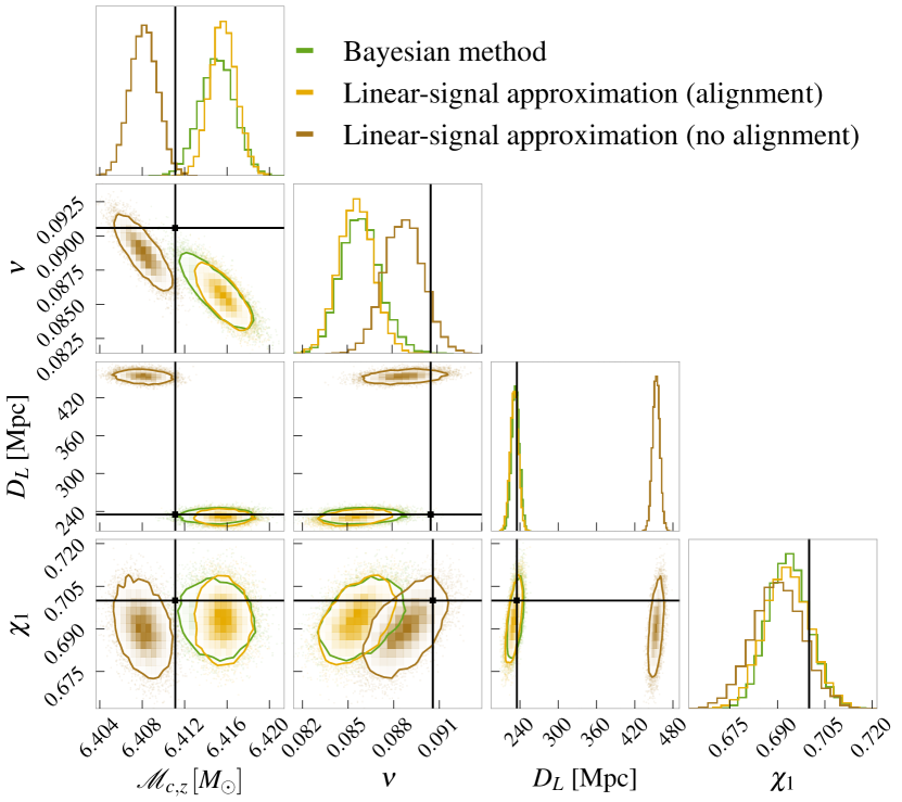
Figure 3: Comparison of the posterior distributions for the chirp mass, symmetric mass ratio, luminosity distance, and primary spin magnitude for Binary 1 with parameters given in Table 1 and in the O5 detector network. The distributions obtained from a Bayesian parameter estimation using Bilby are shown in green. The estimates from the LSA with and without the minimization procedure (12) (alignment) are shown in orange and brown, respectively. The black cross-hairs show the true injected value. The parameter estimation is performed by injecting a SEOBNRv5PHM signal and recovering it with the IMRPhenomXPHM waveforms. The Bayesian posteriors are accurately represented by the LSA when the alignment is enforced.

As a representative case to compare results between the Bayesian method, and the LSA with and without the optimization procedure of Eq. (12), we consider a BBH with parameters given in Table 1, and denoted as Binary 1 in the O5 detector network. In Fig. 3, we show the posterior distributions for selected parameters, namely, $\mathcal{M}_{c}$, $\nu$, $D_{L}$, and $\chi_{1}$, using the Bayesian analysis and the LSA estimate for the errors and biases computed from Eq. (10) and Eq. (11), respectively. The full Bayesian posterior estimates are shown in green. The LSA posterior distributions are multidimensional normal distributions centered at the biased value with the covariance matrix given by Eq. (10). The curves in orange show the distributions when the biases are estimated by minimizing the mismatch between the waveforms (see Eq. (13)), while the ones in brown are the estimates when the minimization is not performed (as it is typically done in the literature; Eq. (11)). Since the covariance matrix is approximately the same in a neighborhood, the posterior widths are similar. However, the predicted bias differs substantially between the two procedures. The effect on the estimation for the distance bias is especially noticeable, with the traditional method predicting a $\approx 50\%$ bias when it is unbiased in actuality. This would be of particular importance for cosmology studies where the traditional estimates done in the literature would be overly pessimistic. The contours show the 90% credible intervals of the parameters.

We now briefly discuss the validity of the LSA. Even though we find excellent agreement between the LSA and the Bayesian analysis for this fiducial case, it is important to keep in mind that the estimates are approximate. Particularly, both the FIM and the bias formula (Eq. (13)) are derived under the assumption that a waveform model can be expanded linearly in its parameters. While the FIM approximation improves with increasing SNR, with higher order contributions scaling as $\mathcal{O}(1/\acs{SNR})$, the bias is independent of the SNR both in the linear approximation and the full likelihood. For the LSA, this can be easily gauged from the bias equation, Eq. (13), which is independent of the distance and/or simple scaling of the PSD. For the Bayesian analysis, one can conclude from Eq. (7) that a simple scaling of the PSD will not affect the stationary points. Therefore, the point in the parameter space where the likelihood peaks remains constant. This means that the error in the bias computation is also constant. In addition, note that we are interested in the bias in units of the statistical errors. Hence, while the measurement becomes better with improving sensitivity (or larger SNR), the error in the systematic bias estimated using LSA becomes more important. A priori it is difficult to know the range of the sweet spot where both approximations hold. However, the event shown in Fig. 3 has an $\acs{SNR}\sim 75$ and we also observe similar agreement in the A# network where the event has an $\acs{SNR}\sim 220$ (see Table 1) prompting us to make the reasonable assertion that the LSA is most trustworthy for such ranges of the SNR. We were not able to directly compare the Bayesian results in the XG network with the LSA estimates because as we explain in Sec. III.1, the former assumed an L-shaped interferometer for ET while the latter was done using a triangular ET configuration. We would also like to stress that one would expect the LSA to hold when the mismatch between two waveform models is not too large. For the case illustrated above, we find the mismatch, $\mathcal{M}\sim 3\%$. However, the binaries that are considered in Sec. IV and Sec. V can have much larger mismatches and a more detailed analysis is required to quantify the validity of the LSA as a function of the mismatch which is beyond the scope of this study.

III.4 Hierarchical Bayesian analysis

We now discuss the method, which we employ in Sec. IV to understand the impact of the biases on the inference of the properties of the BBH population. Given a set of $N_{\rm obs}$ observed data $\{d_{i}\}$, we can estimate the underlying distribution of parameters that generated it through a hierarchical Bayesian analysis. We denote by $\vartheta$ ($\subset\bm{\vartheta}$) the set of parameters, whose distribution we wish to infer. Assuming a form for the number density of observed events, $\frac{{\rm d}N}{{\rm d}\vartheta}(\Lambda)$, that depends on hyperparameters $\Lambda$, the posterior on the latter is given by [135, 136]

$$p(\Lambda|\{d_{i}\})\propto\pi(\Lambda)e^{-N(\Lambda)}\prod_{i=1}^{N_{\rm obs}}\int\frac{{\rm d}N}{{\rm d}\vartheta}(\Lambda)\frac{p(\vartheta|d_{i})}{\pi_{\text{PE}}(\Theta)}{\rm d}\vartheta,$$ (14)

where $p(\vartheta|d_{i})$ is the single-event posterior, $\pi_{\text{PE}}(\vartheta)$ is the prior used for parameter estimation, $\pi(\Lambda)$ is the prior on the hyperparameters, and $N(\Lambda)$ is the total number of events, defined as

$$N(\Lambda)=\int\frac{{\rm d}N}{{\rm d}\vartheta}(\Lambda){\rm d}\vartheta.$$ (15)

In the analysis of real data, the above equation must be modified to include selection effects. We interpret ${\rm d}N/{\rm d}\vartheta$ as the rate density of the full population, and modify the argument of the exponential to $p_{\rm det}(\Lambda)N(\Lambda)$, where $p_{\rm det}(\Lambda)$ is the probability of detection of a source, averaged over the population model. In the analysis performed here, we instead approximate selection as a hard cut on the intrinsic SNR of the source. In this model, selection is now defined on the source parameters, not the data, and the above equation can be used directly, but ${\rm d}N/{\rm d}\vartheta$ must now be interpreted as the rate density in this observed portion of the population. This approach, which is common in the literature, ignores the fuzziness at the detection horizon that arises from instrumental noise, but will give quantitatively reliable and unbiased results, provided the data is simulated from the same model. In Eq. (14), we use the proportionality symbol instead of the equality one because we have omitted numerical factors that depend on the observed data $\{d_{i}\}$, but not on $\Lambda$, i.e., the individual event evidences and the overall model evidence. These factors are required to perform model selection, but are unimportant when the goal is to obtain the posterior distribution on $\Lambda$.

We perform a hierarchical Bayesian analysis for each source parameter separately, i.e., $\chi_{1}$, $q$, $\cos\theta_{1}$, and $\mathcal{M}_{c}$, so that ${{\rm d}N}/{{\rm d}\vartheta}$ is a one-dimensional function. This yields optimistic measurements for the number densities as compared to the full inference, but allows us to have a quick assessment of the impact of systematic biases on population inference. Adopting the approach of Toubiana et al. [137], we describe the number density of observed events, ${{\rm d}N}/{{\rm d}\vartheta}(\Lambda)$, as a piece-wise linear function. The extremities of the $\vartheta$ range over which we perform the inference are fixed, and determined by the minimum and maximum samples present in the data. Thus, our hyperparameters are: the values of the number densities at the extremities, the number of knots, their positions and the value of the number density at the knots. The number density at any point is then obtained by linear interpolation. We stress that the number of knots is a free parameter of the model, and is inferred by using a reversible-jump Markov chain Monte-Carlo algorithm [138]. In this way, the complexity of the model is determined by the data itself.

For a given detector network, we perform population inference on a mock catalog with systematic biases and on one without, generated as follows.

1. We draw the parameters $\vartheta_{0}$ from the population model described in Sec. IV and select those with SNR above a given threshold.

2. We compute the measurement error and the systematic bias for all observable events using the LSA, as described in Sec. III.2.

3. For the catalog with systematic biases, we shift the true parameters by $\delta\vartheta_{bf}$ to obtain the biased parameters, $\vartheta_{bf}$.

4. For each event $\vartheta_{i}$, we attribute a measurement error $\sigma_{i}$ drawn randomly among the set of computed measurement errors, allowing for replacement.

5. We draw a noisy measurement $\vartheta_{n,i}$ of each event from a Gaussian centered at $\vartheta_{i}$ ($\vartheta_{bf,i}$ for the biased catalog), with standard deviation given by the error drawn in step 4.

Under the LSA, the posterior distribution on $\vartheta$ is a truncated Gaussian:

$$p(\vartheta|\vartheta_{n,i})=\frac{2\exp\left[-\frac{1}{2}\frac{(\vartheta-\vartheta_{n,i})^{2}}{\sigma_{i}^{2}}\right]}{\sqrt{2\pi}\sigma_{i}\left[\operatorname{erf}\left(\frac{\vartheta_{\rm max}-\vartheta_{n,i}}{2\sigma_{i}}\right)+\operatorname{erf}\left(\frac{\vartheta_{n,i}-\vartheta_{\rm min}}{2\sigma_{i}}\right)\right]},$$ (16)

where $\vartheta_{\rm min}$ and $\vartheta_{\rm max}$ are the boundaries of the prior domain on $\vartheta$. The purpose of the randomization of the errors (step 4) is to remove the dependency on $\vartheta$ from the standard deviation entering the posterior distribution. If we were to use the corresponding value predicted by the FIM for each event, we would have to account for the complicated dependency of $\sigma$ on $\vartheta$, and the posterior on $\vartheta$ would no longer be a Gaussian, requiring to go to beyond quadratic order in the LSA. Moreover, $\sigma$ would also depend on the remaining parameters in $\bm{\vartheta}$, and, by performing the inference on a single parameter, we would not be accounting for this dependence correctly, making our analysis not self-consistent. However, we observe that, for $\vartheta=q$ or $\chi_{1}$ or $\cos\theta_{1}$, the amount by which the estimated uncertainty in the parameter varies over the range of our priors is small, so we expect our procedure to yield realistic results for those parameters. Step 5 is crucial to make sure our mock catalog is self-consistent from the statistical point of view. Working in the so-called zero-noise approximation is valid for performing parameter estimation on single mock events, because it is a fair realization of the noise in the detector. On the other hand, having zero noise for all events is no longer a fair realization, and would be valid only if all the events were perfectly measured. Note that, in steps 3 and 5, we allow the biased parameters and the noisy ones to be outside of the prior range. The rationale is that those steps are meant to mimick the behavior of the likelihood function in the presence of systematic biases and noise, which, as a function, does not contain information on the physically allowed range of a given parameter. The posterior in turn is truncated to the prior range, as done explicitly in Eq. (16).

In the hierarchical Bayesian analysis, we take the parameter estimation prior $\pi_{\text{PE}}(\vartheta)$ to be flat in $\vartheta$. Thus, each of the integrands in Eq. (14) is the product of a Gaussian with a piece-wise linear function, and we can perform the integration analytically. This allows us to evade problems related to having an insufficient number of samples when performing Monte-Carlo integration [139] and speeds up the analysis.

IV Systematic biases in the BBH population

In this section, we study the effect of systematic biases on a BBH population. We use the GWTC-3 results [5, 14] only for the distribution of masses. We explore the impact of systematic biases on this LVK-like population, considering the three detector networks introduced in Sec. II.3. We also do a hierarchical Bayesian inference of the underlying population where we re-weight our population distribution to the current LVK distribution of astrophysical BBHs.

IV.1 LVK-like population

We simulate $10^{5}$ binaries in each of the detector networks described in Sec. II.3 up to a redshift $z=3$ using the SEOBNRv5PHM waveform model. Following Borhanian and Sathyaprakash [27], this is around the expected number of BBH mergers per year. We choose a network SNR threshold of 12 for detection and use this to identify the subset of simulated binaries that are in the population observed by each network.

The redshift distribution for the population is drawn from a probability distribution given by

$$p(z)\propto\frac{dV_{c}}{dz}\frac{1}{1+z}\psi(z),$$ (17)

where $dV_{c}/dz$ is a comoving volume element per unit redshift and $\psi(z)$ is the SFR which is taken to be [103]

$$\psi(z)=0.015\frac{(1+z)^{2.7}}{1+[(1+z)/2.9]^{5.6}}\rm M_{\odot}yr^{-1}Mpc^{-3}.$$ (18)

The distribution of the primary source-frame mass is assumed to follow the Power Law + Peak model of Abbott et al. [14] with the parameters fixed to their maximum likelihood values. For completeness and ease of reference, we elucidate the model here. The Power Law + Peak model is given by

$$\begin{split}p(&m_{1}|\lambda_{\rm peak},\alpha_{m},m_{\rm min},m_{\rm max},\mu_{m},\sigma_{m},\delta_{m})\propto\\ &[(1-\lambda_{\rm peak}){\rm PL}(m_{1}|\alpha_{m},m_{\rm max})+\lambda_{\rm peak}\mathcal{N}(m_{1}|\mu_{m},\sigma_{m})]\\ &\times S(m_{1}|m_{\rm min},\delta_{m}),\end{split}$$ (19)

where $\lambda_{\rm peak}$ gives the weight of the peak component, ${\rm PL}(m_{1}|\alpha_{m},m_{\rm min},m_{\rm max})$ is a normalised power-law distribution with spectral index $\alpha_{m}$ and truncated to the range $[m_{\rm min},m_{\rm max}]$, $\mathcal{N}(m_{1}|\mu_{m},\sigma_{m})$ is a normalised Gaussian distribution and finally, $S(m_{1}|m_{\rm min},\delta_{m})$ is a smoothing function defined by

$$S(m|m_{\rm min},\delta_{m})=\begin{cases}&0;\ {\rm if}\;m<m_{\rm min},\\ &[f(m-m_{\rm min},\delta_{m})+1]^{-1};\\ &\ {\rm if}\;m_{\rm min}\leq m\leq m_{\rm min}+\delta_{m},\\ &1;\ {\rm if}\;m>m_{\rm min}+\delta_{m},\end{cases}$$ (20)

with

$$f(m,\delta_{m})=\exp\left(\frac{\delta_{m}}{m}+\frac{\delta_{m}}{m-\delta_{m}}\right).$$ (21)

The maximum likelihood values for the fit to GWTC-3 [14] were $\lambda_{\rm peak}=0.02$, $\alpha_{m}=-3.5$, $m_{\rm min}=4.8M_{\odot}$, $m_{\rm max}=83M_{\odot}$, $\mu_{m}=34M_{\odot}$, $\sigma=1.9M_{\odot}$ and $\delta_{m}=5.4M_{\odot}$. The mass ratio distribution is modeled using a power-law with a smoothing function and takes the form

$$p(q|\beta_{q},m_{1},m_{\rm min},\delta_{m})\propto q^{\beta_{q}}S(qm_{1}|m_{\rm min},\delta_{m})$$ (22)

where the maximum likelihood value for the spectral index $\beta_{q}=0.76$.

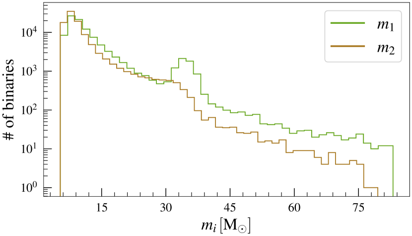
Figure 4: The distribution of component masses for a population of $10^{5}$ BBHs following the astrophysical distribution as determined by the LVK Collaboration.

The analyses performed on GWTC-3 [14] suggest a broad distribution for the spin magnitude, peaking around $0.2$ and falling off to 0 for large spins. However, we are particularly interested in estimating systematic biases for large-spin systems, so we draw the magnitude uniformly between 0 and 1. The analyses on systematic effects are performed on this population, in particular we compute the measurement uncertainties and systematic biases within the LSA for these parameters, but when performing the hierarchical Bayesian analysis, we generate the mock catalog by performing importance sampling on this flat population to obtain a spin distribution in agreement with the results of the DEFAULT model of Abbott et al. [14]. Finally, we assume the spins’ orientation to be distributed isotropically, which is in qualitative agreement with the results on GWTC-3.

The location and orientation of the binary in the plane of the sky is assumed to be randomly distributed. Therefore, the declination angle, $\delta$, right ascension, $\alpha$, and inclination angle, $\iota$, follow the distributions $\cos\delta\in\mathcal{U}[-1,1]$, $\alpha\in\mathcal{U}[0,2\pi]$, and $\cos\theta_{\rm JN}\in\mathcal{U}[-1,1]$, respectively. The polarization angle, $\psi$, and the coalescence phase, $\phi_{c}$, are also drawn from a uniform distribution, $\psi,\phi_{c}\in\mathcal{U}[0,2\pi]$.

We report the SNR distribution of the $10^{5}$ binaries simulated in the three detector networks in Fig. 5. We shade the region below the SNR threshold of 12 in grey. The tail of the three distributions exhibit the $\propto\rho^{-4}$ dependence of the rate of mergers per unit redshift in accordance with the uniform in comoving-volume distribution of sources in the nearby universe. On the other hand, the peak of the distribution correlates with the peak of the SFR, while the initial slope depicts the first generation of stars following the dark ages. While we are limited by the sensitivity of the current detector networks and their upgrades in our ability to observe GWs from the mergers of the first stellar-origin BBHs, the XG network will enable us to study BBH mergers immediately following reionization.

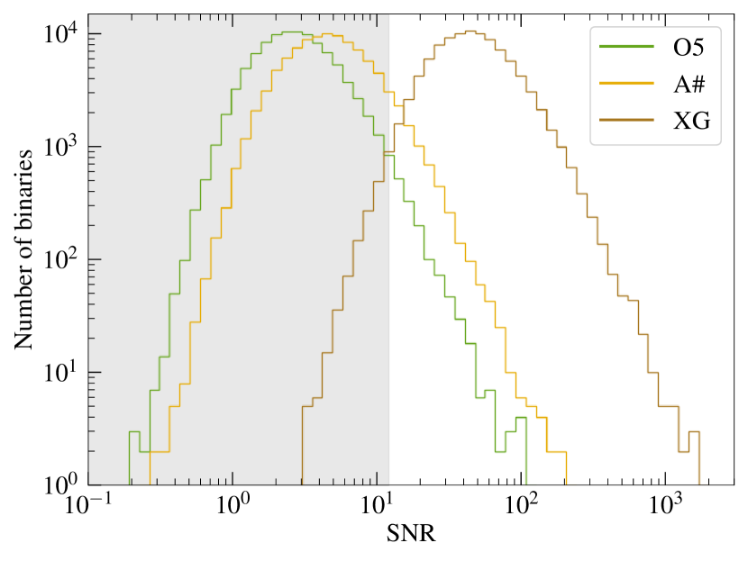
Figure 5: The distribution of the SNRs of the $10^{5}$ BBHs simulated in the three detector networks computed using the IMRPhenomXPHM model. The SNR distribution is similar when using the SEOBNRv5PHM model. We indicate in shaded gray the region with network-SNR threshold below 12.

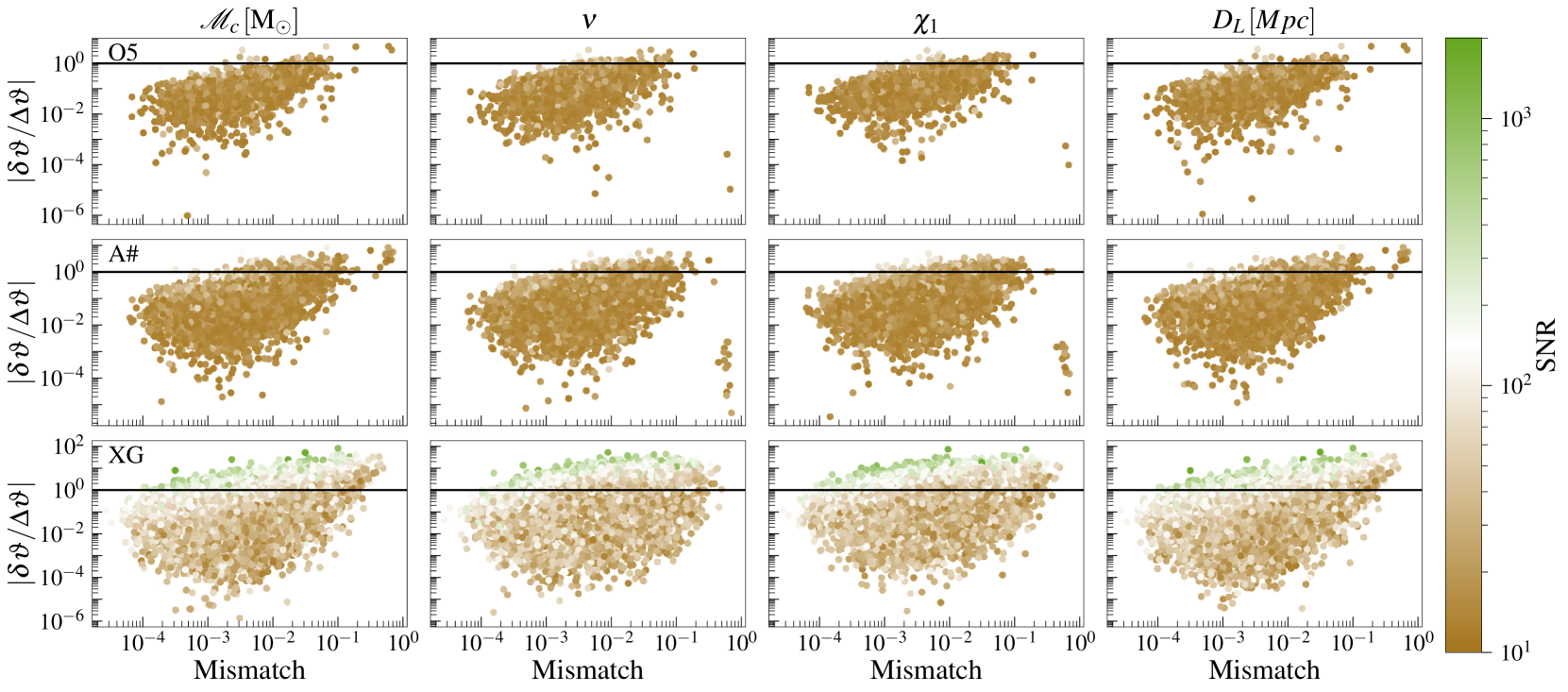
Figure 6: The ratio between the systematic bias and statistical errors, $\delta\vartheta/\Delta\vartheta$, for source-frame chirp mass, symmetric mass ratio, primary spin magnitude, and luminosity distances as a function of the mismatch between SEOBNRv5PHM and IMRPhenomXPHM waveform models for a population of BBH mergers as observed by the LVK. A network SNR threshold of 12 was imposed on the $10^{5}$ binaries in the population resulting in $\sim 1800$, $\sim 8100$, $\sim 99000$ detected events in the O5 (top), A# (middle), and XG (bottom) networks, respectively. The SNRs of the binaries are depicted using the different colorscales. The outlier events in the top and middle panels having the largest mismatches are the heaviest and most distant events with redshifted total mass $>400M_{\odot}$ and redshift $>2$.

IV.2 Systematic bias

In the following, we discuss, at first, the systematic biases for the individual events in the LVK-like population. Then, we carry out a hierarchical Bayesian inference of the population distributions by reweighting the parameter distributions to the LVK distribution. Finally, we determine the type of binaries more likely to be biased, which motivates our analysis of Sec. V.

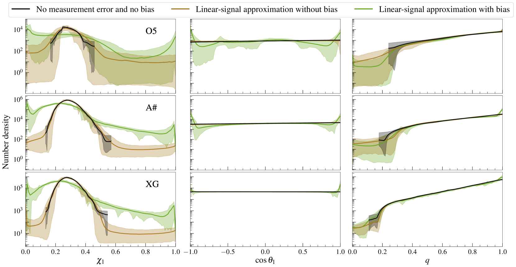
Figure 7: Inferred distribution of $\chi_{1}$, $\cos\theta_{1}$, and $q$ for different detector networks, in the case where the parameters are measured perfectly (black), where there is measurement error but no bias (brown), and where there is measurement error and bias (green). The solid lines show the mean value in a given bin and the shaded areas the $90\%$ confidence intervals. The “no measurement error and no bias” case does not correspond to any realistic scenario and is there to show the underlying distribution of observed events, accounting for Poisson errors. For $\chi_{1}$, when including biases, we observe a shift towards smaller values together with a broadening of the distribution, particularly for A# and XG. For $\cos\theta_{1}$, we observe an excess of events at both ends and for $q$ at $\sim 1$. The distributions in the XG case for those two parameters are less biased because the bias for individual events is smaller in XG.

Variation with mismatch

Armed with the biases in the GW parameters and their measurement errors, we report in Fig. 6 their ratio, $|\delta\vartheta/\Delta\vartheta|$, as a function of the mismatch, $\mathcal{M}$, between SEOBNRv5PHM and IMRPhenomXPHM for the chirp mass, symmetric mass ratio, primary spin magnitude, and luminosity distance. We recall that the biases are computed using Eq. (13). The SNR for the binaries of the population are portrayed using a colorscale with lighter colors representing smaller SNR and vice-versa. A value of $|\delta\vartheta/\Delta\vartheta|>1$ indicates that systematic biases are larger than the typical size of statistical errors. A common feature for all the parameters is a direct correlation between $|\delta\vartheta/\Delta\vartheta|$ and the mismatch. This is intuitive because a larger mismatch implies a greater difference between the two waveform models and, therefore, larger biases assuming the measurement errors do not vary significantly with the mismatch which we find to be broadly true for the population. On the other hand, the colorscale shows that the loudness of a signal is not a guarantee for a dominant systematic effect with quieter signals exhibiting significant systematic biases particularly when the mismatch is greater. This is especially true for the O5 and A$\#$ networks. We provide a complementary plot of $|\delta\vartheta/\Delta\vartheta|$ as a function of the SNR in Fig. 24 in the appendix for the interested reader.

A few events appear as outliers in the figure with large mismatches but extremely small $|\delta\vartheta/\Delta\vartheta|$ for the O5 and A$\#$ networks. These are the heaviest and most distant events with redshifted total masses $>400M_{\odot}$ and redshifts $>2$. As such, these signals are extremely short consisting of only the merger-ringdown. The FIM in these cases is close to singular because the signal does not contain much information resulting in extremely large errors. This suppresses the ratio for every parameter except the luminosity distance in which case the ratio is directly proportional to the mismatch and hence large. The LSA approximation is not reliable for such cases and we should resort to full Bayesian analyses. Nevertheless, we include these binaries in the figure to show their existence in the population observable by these two networks.

Figure 6 also shows that the number of binaries with biased parameters as a fraction of the detected population increases with improving detector sensitivity. This can be simply understood as due to the independence of the overall scale of the PSD in estimating the parameter bias (see Eq. (11)) while the covariance is inversely proportional to it. While an improving detector sensitivity leads to an increase in the total number of binaries that are significantly biased, the increase in the biased fraction has to do with the finite number of stellar origin BBH mergers in the universe. Note that because of different PSD shapes, interferometer designs, and minimum frequencies, the three rows of Fig. 6 are not simply shifted versions of one another. Nevertheless, even for the XG network, only a minority of events are biased with the biased fraction ranging from $10-25\%$ depending on the parameter. For detectors of the current generation, the biased fraction is even smaller with only $\sim 2\%$ and $\sim 2.5\%$ of binaries significantly biased for the O5 and A$\#$ networks respectively. This suggests that biases in parameter estimation will only be of importance for extraordinary individual events rather than for inferring general characteristics of the population. We check this more carefully in the next section.

It is also important to realize that a larger value of $|\delta\vartheta/\Delta\vartheta|$ does not necessarily mean larger value of the absolute bias. For instance, as we will see in Sec. VI, the XG network quite often has smaller absolute biases due to improved low frequency sensitivity where waveform models agree to a greater extent. However, the improved sensitivity reduces the measurement error more than the decrease in the systematic bias resulting in a larger value of $|\delta\vartheta/\Delta\vartheta|$. We will see the effect of this in the next section.

Inferred distributions

Figure 7 shows the inferred number density of events for $\chi_{1}$, $\cos\theta_{1}$, and $q$ for the three detector networks. Solid lines indicate the mean of the number density and colored bands the $90\%$ confidence intervals. The results shown in black correspond to an unphysical scenario where all observed events are perfectly measured. In this case, the only source of uncertainty is the Poisson error due to the finite number of events. The black curves serve as guidance to indicate the underlying distribution on which we perform the inference. We show in brown the case with measurement error and no bias, following the procedure outlined in Sec. III.4. The brown and black shaded areas overlap, with the red encompassing the blue most of the time due to the inclusion of measurement errors, indicating that our procedure yields unbiased results. Thus, differences between the cases without (in brown) and with biases (in green) are due to waveform systematics.

We recall that, when performing the hierarchical Bayesian analysis, we resample the flat $\chi_{1}$ distribution into the distribution inferred by the LVK Collaboration [14] by means of importance sampling. For O5, the biased and non-biased distributions are mostly compatible. However, for A# and XG, we observe that, when including bias, the inferred $\chi_{1}$ distribution is broadened, with the peak being shifted to lower values. The broadening is a consequence of the occurrence of large biases, while the shift happens because the systematic bias typically increases with $\chi_{1}$ (see Fig. 8 and the associated discussion). Events with large spin are more shifted, with a small preference for shifts towards lower $\chi_{1}$, than events with small spins. From the astrophysical point of view, the shift of the peak is rather negligible, but the tail of high spin events would lead to an overestimation of the number of BHs with high spins, by up to two orders of magnitude, potentially challenging formation scenarios.

Figure 8: The percentage of binaries in each $\chi_{1}$ bin with $|\delta\vartheta/\Delta\vartheta|>1$ for different parameters. The top, middle, bottom panels show the percentages for the O5, A#, and XG networks, respectively.

For the tilt angle, we observe an excess at the ends due to events with more precession ($\cos\theta_{1}\sim 0$) being more biased than those with aligned spins. We note that the XG population is less biased than the A# one. This is a consequence of the improvement at detector at low frequencies, which increases the proportion of inspiral signal that is observed, where waveform models agree best, and yielding a less biased estimate of precession effects. We observe a similar behavior for the $q$ distribution. Asymmetric events are more biased than nearly-equal-mass ones, shifting the overall distribution to $q\sim 1$. As for $\cos\theta_{1}$, the XG population is less biased than the A# one. At first glance, this might seem in contradiction with Fig. 6, which shows that the ratio between the systematic bias and statistical error on $\nu$ tends to be larger in the XG case. However, as further discussed in Sec. VI, when comparing the full posteriors, in many cases the result in the XG case is closer to the true value than in the A# case. The ratio between the systematic bias and statistical error is larger for XG because the measurement error decreases more than the bias (in relative terms), but both errors decrease and the fact that the absolute bias is smaller ends up reducing the bias at the level of the population inference. We have also performed hierarchical Bayesian analysis on $\mathcal{M}_{c}$ and found no bias at the level of the population, as expected given that this parameter is typically little biased.

Finally, let us stress again that those results were obtained using the LSA for the measurement error and the systematic bias. As explained in Sec. III.4, we do allow the biased estimate of the parameters to be outside of the physical range, with the idea that this would mimic the likelihood behavior: it is reasonable that the likelihood of an event $\chi_{1}\sim 0$ seems to peak at $\chi_{1}=-0.1$, and when performing parameter estimation we would observe a truncated distribution due to the physical prior. However, in some cases, our formula predicts biases that are orders of magnitude outside of the physical range (e.g $\chi_{1}\sim-10$), most likely indicating that the LSA should not be trusted. Indeed, the LSA relies on the quadratic approximation to the likelihood, which should hold only in a region around the peak of the likelihood, with a better agreement at high SNRs. Thus, the reason for our estimates of the bias with O5 (A#) being so much larger than with XG might also be due to the invalidity of the LSA in some cases. However, observing more of the inspiral certainly contributes, as discussed in more detail in Sec. VI. Overall, we expect the results shown here for XG to be the most reliable.

Which binaries are likely biased?

Having explored the effect of waveform systematics on the full detected LVK-like population and studied the inferred population properties via hierarchical Bayesian inference, we turn our attention to the subset of binaries with significant parameter biases. In the following, we identify the properties of binaries that have a greater susceptibility to systematic biases. To accomplish this, we explore the dependence of the systematic bias as a direct function of the binary parameters. In Fig. 8, we show the percentage of binaries in each $\chi_{1}$ bin with $|\delta\vartheta/\Delta\vartheta|>1$ for various parameters such as the chirp mass, symmetric mass ratio, primary spin magnitude, and luminosity distance. It is immediately clear that the number of binaries with biased parameters increases with increasing $\chi_{1}$. Notice that for current detectors and its upgrades, only a tiny fraction of binaries ($\lesssim 1\%$) have biased parameters when $\chi_{1}<0.4$. Even for highly spinning binaries, the biased percent is less than 10%. In contrast, we observe that a relatively large fraction ($10-25\%$) of the binaries have biased parameters in the XG network even when $\chi<0.4$.

Before ending this section, we remark that the results for the systematic biases of the LVK-like population have been obtained by comparing two state-of-the-art quasi-circular, spin-precessing, multipolar waveform models. However, when assessing the accuracy of the waveform models, more robust and definitive results can be achieved when comparing models to NR waveforms. We plan to carry out such a study in the near future, although it will be limited by the number of NR waveforms and their length.

V Systematic biases across binary parameter space

In Sec. IV, the general properties of systematic bias across an LVK-like BBH population were explored. Here, we consider an agnostic BBH population in order to explore a wider region of the binary parameter space and identify the regions with greater susceptibility to systematic biases.

Figure 9: Comparison of the LVK-like population and distribution of exploratory binaries.

We sample uniformly in the total redshifted mass, $M^{z}\in\mathcal{U}(10,200)[M_{\odot}]$, and inverse mass ratio, $1/q\in\mathcal{U}(1,30)$. However, we impose a constraint on the mass of the lighter object, $m_{2}\geq 5M_{\odot}$, and only select those binaries that satisfy this constraint. This results in a non-uniform distribution in the two masses. Regardless, in this section, our interest is not in any particular distribution of parameters but rather with the coverage of the parameter space. Exploring the region of large inverse mass-ratio is interesting since the waveform models considered here are expected to differ more in this part of the parameter space due to differences in the models’ calibration. For SEOBNRv5PHM, SXS NR simulations for aligned-spin systems at $1/q\geq 15$ and a non-spinning simulation at $1/q\geq 30$ were included in the calibration of the model, and second-order gravitational self-force information was incorporated, improving the reliability of the model at large $1/q$ [52]. An example of the different behaviour of the models for large $1/q$ is shown in Figure 21 of Pompili et al. [50], which illustrates the differences in parameter recovery for a large inverse mass-ratio NR simulation is shown between the aligned-spin versions of SEOBNRv5PHM and IMRPhenomXPHM, with SEOBNRv5PHM being more reliable in the recovery of the parameters.

Due to the lack of calibration to precessing NR waveforms in both waveform models, we expect waveform models to have greater differences for large $\chi_{\rm p}$ values as evident from the mismatch plot of Fig. 10 in Ramos-Buades et al. [51]. Therefore, it is of interest to understand the behavior of systematic biases in these parts of parameter space. Thus, we create a sample of binaries having a uniform distribution in $\chi_{\rm p}$ (the LVK-like population, in turn, disfavors large values of $\chi_{\rm p}$). To do this, we generate a large set of samples for the spin magnitudes and tilt angles from the precessing prior and retain a subset of these samples such that the resulting distribution in $\chi_{\rm p}$ is uniform. This selection procedure has a negligible effect on the distribution of spin magnitude and tilt of the secondary companion while giving greater weight to large and in-plane spin for the primary companion. We draw 50,000 binaries using this procedure to cover the binary parameter space. A comparison in the $1/q-\chi_{\rm eff}$ and $1/q-\chi_{\rm p}$ planes between the LVK-like and the agnostic population is shown in Fig. 9.

The distributions of all other parameters are the same as for the LVK-like population, except for the distance, which is kept fixed at $D_{L}=235\,\rm Mpc$ while computing the measurement errors and biases. However, errors have a simple scaling with the distance for given redshifted masses, while the biases remain unaffected, and we use it to obtain results at other distances.

Bias horizon

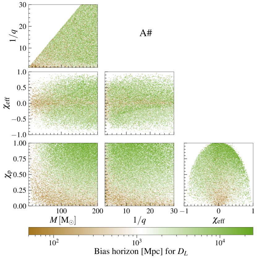
Figure 10: The scatter shows the distribution of the 50,000 binaries in the parameter space represented in Fig. 9, while the color scale shows the distance to which the $D_{L}$ parameter is biased ($\delta D_{L}/\Delta D_{L}\geq 1$) for the O5 (left) and A# (right) networks. Systematic biases become less important if a binary is at a larger distance since measurement precision decreases with distance. Therefore, a large bias horizon signifies that a given parameter ($D_{L}$ in this case) is measured well enough for systematic biases to be important even at such large distances. Notice that the binaries are biased up to a greater distance in the A# network compared to the O5 network due its greater sensitivity, and the resultant improvement in measurement precision.

Figure 11: Same as Fig. 10 for the XG network. BBHs observed with the XG network are biased up to a greater distance than those observed with either the O5 or A# networks, due its greater sensitivity, and the resultant improvement in measurement precision, with a majority of the binaries having a bias horizon $\geq 25\,\rm Gpc$ ($z\approx 3$) beyond which stellar-origin BBHs are not expected to exist.

We compute the biases and the measurement errors on the parameter set $\bm{\vartheta}$ for the 50,000 binaries considered in this section under the LSA as was done in Sec. IV. The ratio $\delta\vartheta/\Delta\vartheta$ of systematic errors to statistical errors is a function of the distance to a binary through the dependence of the statistical error $\Delta\vartheta\sim D_{L}$. We exploit this to calculate the distance at which the ratio $\delta\vartheta/\Delta\vartheta=1$ for any given parameter. Since the measurement errors for a binary with given redshifted parameters increase with its distance, systematic biases will become less important the farther the binary is located. Hence, the distance at which $\delta\vartheta/\Delta\vartheta=1$ is a measure of the bias horizon, i.e., the maximum distance up to which systematic biases dominate statistical errors. Given that the biases and errors for each binary parameter are different, the bias horizons for different GW parameters are also different.

We show the bias horizon for the $D_{L}$ parameter in Fig. 10 for the O5 (left) and A# (right) networks, while that for the XG network is shown in Fig. 11. The distribution of the 50,000 binaries in the 4D space given by $\{M^{z},1/q,\chi_{\rm eff},\chi_{\rm p}\}$ is illustrated by projecting them into 2D subspaces. The bias horizon for each binary is shown by the color bar. The bias horizon increases with increasing detector sensitivity implying that systematic biases will be prevalent up to greater distances. In particular, the majority of the binaries in the XG network have $D_{L}$ bias horizons exceeding $25\,\rm Gpc$ ($z\approx 3$), the distance around which the first stars formed. This is qualitatively different from the conclusions of Sec. IV.2, in particular Fig. 6, where all the binaries have $z\leq 3$ but $\sim 75\%$ of them are not systematic-error dominated. This is due to the different distributions of the parameters in this section compared to the LVK-like population. Particularly, the majority of the binaries considered in this section are highly asymmetric with large redshifted masses. Moreover, a uniform distribution in $\chi_{\rm p}$ leads to a large fraction of highly spinning binaries. We gather from Fig. 8 that systematic biases are more prevalant for such binaries. Note that the boundary in the $\chi_{\rm eff}-\chi_{\rm p}$ space is physical and is a result of the maximum value of the spin magnitude being 1. When comparing the biases for a given binary for different detector networks, it is important to keep in mind that a larger value of the ratio $\delta\vartheta/\Delta\vartheta$ for a better detector network need not be necessarily due to a bigger $\delta\vartheta$, but rather a much more precise measurement (see Sec. IV.2 for further discussion).

We also observe that the importance of systematic biases depend on the parameter space inhabited by the binaries. For instance, from the $\chi_{\rm eff}-\chi_{\rm p}$ space, it is clear that binaries with small spins have smaller $D_{L}$ bias horizon compared to binaries with large $\chi_{\rm eff}$ and/or $\chi_{\rm p}$, with the binaries lying on the parameter space boundary having the largest $D_{L}$ bias horizon. Similarly, one can also observe that for positive $\chi_{\rm eff}$ the bias horizon at large $\chi_{\rm p}$ is higher than for $\chi_{\rm eff}<0$. This can be intuited from Fig. 13 of Pompili et al. [50] which shows that the mismatch is larger for positive $\chi_{\rm eff}$ compared to negative $\chi_{\rm eff}$. Highly precessing binaries with aligned spins have greater $D_{L}$ bias horizon compared to similarly highly precessing but with anti-aligned spins. Along the same lines, we also observe that binaries with large total masses and inverse mass ratios have larger $D_{L}$ bias horizons. Note that we intentionally do not talk about properties relating to the distribution of binaries in the parameter space since they do not follow any physically motivated parameter distributions. We report the bias horizon for $\chi_{1}$ in Figs. 26 and 27 of the Appendix. They broadly show the same dependence across the parameter space although, the quantitative values of the bias horizon are different for each binary parameter.

VI Impact of systematics on the science of individual events

Until now, we have discussed the effect of systematic biases for the LVK-like population in Sec. IV, and explored systematic biases across parameter space within the LSA in Sec. V. In recent years a number of studies have emphasized the science objectives that can be accomplished using GWs in the near future [140, 30, 29]. In this section, we consider a few of those science applications. We then handpick three binaries (see Table 1) with very relevant science potential and discuss the effects of systematic biases on various science objectives. The majority of the results in this section are obtained using a full Bayesian analysis except where pointed out.

VI.1 Science objectives

In the following, we introduce the science applications that will be considered in this section.

1. Cosmology: There exists a tension, at the level of $4.4\sigma$, between the value of the Hubble-Lemaître parameter, $H_{0}$, measured at high redshift from the cosmic microwave background [107], and measured using the local distance ladder comprising Cepheid variables and type Ia supernova [141]. The emergence of GW astronomy provides an avenue for an independent measurement of the Hubble-Lemaître parameter, which could importantly contribute to resolving this tension. Indeed, GWs have already provided multiple independent measurements, albeit not yet at an accuracy to resolve the tension [19, 20, 142, 143, 144].

   A measurement of $H_{0}$ requires both the luminosity distance and redshift of a source to be estimated. GW observations provide the former, but additional data or assumptions are required to provide the latter. For GW observations accompanied with an EM counterpart, primarily binaries containing NSs, the redshift information is provided by spectroscopic/photometric observations of the host galaxy [145, 146]. In binary neutron star (BNS) or neutron-star–black-hole (NSBH) observations, NS tides can be used to provide an independent redshift measurement [147, 148, 149] and, thereby, infer $H_{0}$ [150, 151, 152, 153]. Alternatively, features in the mass distribution of compact binaries can be exploited [154, 155, 156, 157]. Finally, a statistical measurement of the redshift using galaxy catalogues [158, 159, 36, 160, 161, 162] or galaxy cross-correlation techniques [163, 164, 165] can be employed.

   Here, the focus is on the last technique, which can be applied to BBH systems, but relies on an accurate measurement of the distance and sky position. An indirect effect on cosmological inference due to inaccurate determination of the mass distribution will be discussed in the following subsections.

   Events that have the smallest volumetric uncertainties are the most informative systems for statistical measurements using galaxy catalogues [20, 160]. This can be intuitively understood as follows: if there is a single galaxy in the localization volume of a GW event, and one assumes that the event originated in a galaxy, then there is unit probability that the identified galaxy hosted the event and the redshift is known as well as the galaxy redshift. On the other hand, if the volumetric localization of the GW event is poor and there are a large number of galaxies that are potential hosts, the redshift distribution would essentially be uniform, getting contributions from each possible host. All three events studied here are prime candidates for such a method due to their asymmetrical component masses that make distance estimates more precise than analogous comparable mass mergers. This is because of a greater contribution from subdominant harmonics that break the distance-inclination degeneracy. Spin precession also helps in breaking this degeneracy since it mixes different modes in the inertial frame.

2. Lower mass gap: The nature of compact objects with masses between $2\rm\,M_{\odot}-3\rm\,M_{\odot}$ can have wide-ranging consequences in fundamental physics — from the physics of nuclear matter to primordial BH formation mechanisms — and astrophysics — from hierarchical formation probabilities to the proportion of rapidly spinning NSs. The LVK Collaboration has observed two events where one of the components of the binary unambiguously lies in this mass range — GW190814 [166] and GW200210_092254 [5]. Tidal effects on GW waveforms in highly asymmetric mergers hosting candidate NSs, such as the Binary 1 system, are minimal. Therefore, indirect constraints on the nature of the secondary and the binary’s formation history are derived indirectly from their mass and spin measurements.

   The existence of ultra-heavy NSs has consequences for the nuclear equation of state (EoS) at a few times the nuclear saturation density [167] with the possibility of nontrivial structures in the speed-of-sound relation and related phase transition phenomena [168, 169] or rapidly rotating NSs stabilized against collapse by its rotation [170, 171, 172, 173]. On the other hand, BHs in this mass range will inform the primordial BH formation scenarios [174, 175, 176] and hierarchical mergers in dense environments [177, 178, 179, 180, 181]. It is also proposed that the secondary gains mass due to accretion either prior to a supernova explosion [182] or following it [183]. In all of these scenarios, accurate measurements of the mass and spin are essential to further the storyline.

3. PISN mass-gap: In the mass range of about $50\mbox{--}120\rm\,M_{\odot}$, there is expected to be a dearth of stellar origin BHs. This is because main sequence stars with masses heavier than $\sim 120\rm\,M_{\odot}$ have core temperatures that facilitate electron-positron pair production which lead to a decrease in radiation pressure in the core of the star, causing explosive oxygen burning, and a resultant disruption of the entire star. This process, known as a PISN process, does not leave behind a remnant, thereby producing a dearth of BHs above $\sim 60\rm\,M_{\odot}$. However, if the mass of the main sequence star is greater than $\sim 250\rm\,M_{\odot}$, all the heavy elements undergo photo-disintegration, first to alpha particles and then further. This reduces the radiation pressure causing the star to implode forming a BH with mass greater than $\sim 120\rm\,M_{\odot}$.

   The determination of the boundaries of this mass-gap can inform the physics of PISN, such as the $\prescript{12}{}{C}(\alpha,\gamma)\prescript{16}{}{O}$ reaction rate [35, 184], and the role of stellar rotation [185]. Other astrophysical processes such as mass reversal, mass growth due to accretion, and hierarchical mergers can result in the formation of BHs that populate this mass gap.

4. Spin Morphology: The spin distribution of BHs in binaries provides crucial information on their formation channels. Upcoming observing runs of LVK detectors and XG observatories will measure the spins of compact binaries to ever greater precision. This will help to constrain the spin distribution of astrophysical BBH populations and their formation channels. For instance, binaries formed via isolated evolution tend to have their spins aligned with the orbital angular momentum, while those formed dynamically are likely to have an isotropic spin distribution. Similarly, hierarchical formation is expected to produce larger spins compared to stellar collapse. However, given that the spin measurements are expected to be precise, it is crucial for them to be accurate as well to allow unbiased inference of the source properties of the underlying population. We have already discussed the indirect effects of the spin measurement on the inference of the nature of the secondary component of the Binary 1 system in Sec. VI.3.2. In the following, we discuss the systematic biases on the spin for another binary system.

   The origin of massive BBHs, particularly those filling the upper mass-gap, can be traced using their effective spin, $\chi_{\rm eff}$, and spin-precession, $\chi_{\rm p}$, parameters. A hierarchical formation mechanism leads to large component spins since the remnant of the previous merger is expected to be spinning.

   While the $\chi_{\rm eff}$ and $\chi_{\rm p}$ parameters can broadly inform and differentiate between an isolated and dynamical formation channel, an accurate measurement of the tilts of the two spin vectors with respect to the orbital angular momentum, $\theta_{1}$ and $\theta_{2}$, and their relative orientations in the orbital plane, $\phi_{12}$, provide detailed knowledge of the formation mechanisms and spin distributions of the BBH merger population. Precessing binaries exist in different spin morphologies [186, 187, 188, 189] due to spin-orbit resonances [190]. Therefore, precessing binaries can exist in subpopulations characterized by their spin morphology depending on their tilt angles at formation [191, 192, 193, 194, 195, 196]. Recent efforts have gone in to better understanding the spin-precession dynamics [197] and the ability of current detectors to measure spin-precession effects on the waveform [198]. There have also been efforts to probe whether the BBHs detected by the LVK Collaboration are associated with a particular spin morphology [199] as well as studies on the capability of current detectors at improved sensitivities to distinguish different spin morphologies [200, 201].

5. Remnant quantites: The properties of the remnant BH following a BBH merger can be determined from its binary parameters. However, the nonlinear merger makes a fully analytical calculation intractable. As such, estimates of the final mass ($M_{f}$) and spin ($\chi_{f}$) of the remnant include information from NR. Several studies have proposed fits for the remnant quantities for non-precessing binaries [202, 203]. In the precessing case, the final mass is found to agree very well using a non-precessing formula but the same does not hold true for the final spin where the in-plane spin components are important [204, 205]. Some simple arguments to include in-plane contributions have also been proposed in the literature [206, 207, 208]. Such arguments have been used to augment the non-precessing final spin estimates [202, 203]. A surrogate model for the final spin using NR has also been proposed for moderate mass ratios [205]. In this paper, the reported final mass estimates are the average of the non-precessing fits in Refs. [202, 203]. The final spin is computed by averaging the estimates of Refs.[202, 203, 208] with in-plane spin augmentations for the non-precessing fits of Refs.[202, 203].

   Such estimates of the remnant quantities are important not only for modeling the ringdown in inspiral-merger-ringdown waveforms, but also for probing the dynamics of the merger and the nature of the remnant. The ringdown of a Kerr BH is described by quasi-normal modes whose complex frequencies are determined from the properties of the final stationary BH. Therefore, the ringdown signal can be used to estimate the mass and spin of the final remnant independently. The remnant quantities can be affected by deviations from GR which can modify the radiated energy and angular momentum as well as an exotic remnant which will have a modified spectrum, resulting in inconsistent estimates from the ringdown signal and NR inspired fits. Such consistency tests have been performed for GW150914 [21, 209] and GW190521 [210, 211]. With improving detector sensitivities, such tests form an important part of null hypothesis tests of GR.

6. Maximal BH spins: Obtaining accurate spin measurements from astrophysical BHs is a non-trivial endeavor for which different electromagnetic approaches exist. In the context of stellar-mass BHs, it is possible to apply the continuum fitting method or reflection spectroscopy to X-ray observations [212, 213] . However, modeling the astrophysical environment is non-trivial and can introduce systematic effects. GW measurements provide a novel way to measure BH spins, and due to their vacuum environment, might be easier and more robust to model. While the spin distribution of BBH systems can provide valuable information about their formation channels, an individual event with very high spins, especially if close to extremal Kerr, would be of great scientific interest. For instance, due to the cosmic censorship hypothesis, no naked singularities should exist, which implies that BHs should not spin above $a>1$. Moreover, quasi-normal modes of a rapidly rotating BH become long-lived, which could lead to turbulence phenomena [214].

VI.2 Handpicked binary black holes

We pick three asymmetric and precessing systems out of which one has low total mass and two have large total masses. These systems have some precedence in the current LVK-TCs, though they are not the most common events. We pick them due to their science potential and to explore the parts of the parameter space that are expected to be considerably affected by systematic biases. The parameters of these systems, their SNRs in the different detector networks, and their science objectives are listed in Table 1. We now discuss the properties of these systems and their analogs in the LVK-TCs.

• Binary 1: highly asymmetric, spin-precessing, low total-mass binary. This system is modeled after GW190814 and has masses, distance, and inclination compatible with the measured values [166]. While GW190814 has no measurable spin precession, the system we consider is highly precessing. This is a reasonable choice because a dynamical capture or hierarchical merger are widely accepted as possible formation channels for GW190814 and these channels can produce highly precessing binaries. The merger rate of such systems is estimated to be $7^{+16}_{-6}\,\rm Gpc^{-3}\,yr^{-1}$. Hence, even a pessimistic merger rate of $1\,\rm Gpc^{-3}\,yr^{-1}$ equates to more than 400 such mergers within a redshift of 3 each year. With planned and future observatories, a handful of these mergers will be observed with large SNRs.

• Binary 2: rather asymmetric, nonprecessing, high total-mass binary. Among the LVK observations, the candidate events GW190403_051519 [6] and GW200208_222617 [5] have properties similar to this system. Both the candidates are asymmetric binaries with large effective spins indicating that the spins are aligned to the orbital angular momentum. The median of the posterior distribution of the primary spin magnitude for GW190403_051519 is $\chi_{1}=0.89$ while the probability that the primary spin of GW200208_222617 is $\chi_{1}>0.8$ is 51%. The primary components for both candidates also have a considerable probability of being in the upper mass-gap. While these events were marginal detections with moderate astrophysical significance, their science potential is immense and confident detections of similar systems in the future will be invaluable. From a modeling perspective, it is also an interesting region of the parameter space to probe, because different state-of-the-art waveform models have significant mismatches for binaries with large aligned spins.

• Binary 3: rather asymmetric, spin-precessing, high total-mass binary. This system has the same parameters as Binary 2 except for the spins which are now misaligned with respect to the orbital angular momentum. The origin and associated formation channels for such systems through stellar evolution is highly uncertain [215, 216, 217, 218, 219]. Nonetheless, the current observations provide sufficient evidence for the existence of such systems and, therefore, it is essential to understand whether current waveform models have the necessary accuracy to study such mergers.

		Binary 1: highly asymmetric, spin-precessing, low total mass	Binary 2: rather asymmetric, nonprecessing, high total mass	Binary 3: rather asymmetric, spin-precessing, high total mass
Parameters	$m_{1}[M_{\odot}]$	23.2	61.8	61.8
	$m_{2}[M_{\odot}]$	2.6	9.5	9.5
	$\chi_{1}$	0.7	0.9	0.9
	$\chi_{2}$	0.4	0.8	0.3
	$\theta_{1}[^{\circ}]$	40	0	140
	$\theta_{2}[^{\circ}]$	40	0	120
	$\chi_{\rm eff}$	0.51	0.89	-0.43
	$\chi_{\rm p}$	0.45	0	0.77
Network SNR	O5	75.3	222	119
	A#	137	405	219
	XG	1040	3150	2490
Science cases	Cosmology	✓	✓	✓
	Lower mass gap	✓	✗	✗
	PISN mass gap	✗	✓	✓
	Spin morphology	✓	✗	✓
	Remnant quantities	✓	✓	✓
	Maximally spinning secondary	✗	✓	✓

Table 1: We list the properties of the three systems that we study using Bayesian analysis in Sec: VI. The top row lists the intrinsic parameters of the systems, the middle row enumerates the SNR of the systems in the three detector networks used, and the last row illustrates the science applications associated with each system.

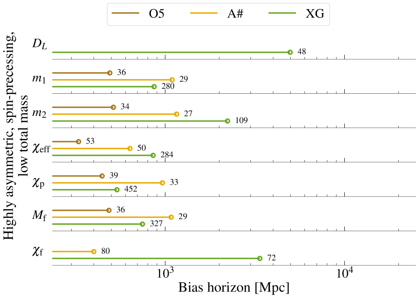
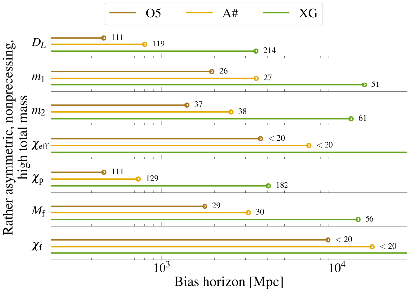
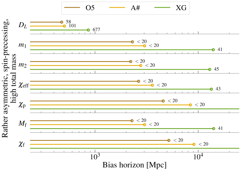
Figure 12: We show the bias horizon for the most relevant parameters of the three systems (from top to bottom panels) for the three different networks. The colored lines indicate up to which distance the systematic error of a parameter is outside the 90 % credible interval of the posterior and thus describes biased parameters. The circles at the end of each line indicate the bias horizon, which is the distance where it is at 90 %. The number at the end of each line reports the SNR at that distance. Note that there is a cutoff at 25 Gpc (lines without circle), and that we only explicitly show SNRs up to 20.

For all three events we perform a full Bayesian analysis placing them at a luminosity distance of 235 Mpc. While BBH mergers at this distance are certainly possible and have been observed, they are few in number and the majority of events will originate from larger distances. On the other hand, the SNR for events that are sufficiently far away will be small and the systematic biases will be inconsequential compared to the measurement errors. It is therefore desirable to know the maximum distance up to which a given science objective will be affected due to biases in parameter estimation. However, it is infeasible to repeat the full parameter estimation calculation for multiple distances. For that reason, we model the posterior distribution using its median and covariance. This is equivalent to the LSA approximation in the large SNR limit. In this limit, the bias is independent of the strength of the signal while the covariance increases with the square of the distance. We compute the bias horizon for the three sources and these are shown in Fig. 12. A cursory look at the SNRs required for a parameter to be biased reveals that biases could be present for much smaller SNRs than what is simulated here. Below, we will discuss the implications of these results in the context of various science applications. The posteriors for events with low SNR are not well approximated by a Normal distribution. The simple scaling argument employed here fails for such cases. Therefore, for parameters for which the SNRs the bias horizon is $<20$, we do not quote the exact value but rather denote it with an inequality sign. Similarly, we do not show the exact projected distances if they are larger than $25\,\rm Gpc$ ($z\sim 3$). Note that there is an implicit assumption in this scaling argument that the detector-frame masses are constant. For large distances, the source-frame masses would be materially smaller. Therefore, the binaries considered may no longer be appropriate for science objectives related to the source-frame mass. If, in turn, these binaries are placed at a larger distance, while keeping the source-frame quantities constant, they will have a larger detector-frame total mass and, consequently, fewer GW cycles in the detectable band. Since the differences between various waveform models are greater closer to the merger, one expects that the bias will be larger for such systems compared to the scaled binaries. For instance, it can be seen from Figs. 10 and  11 that the bias horizon is generally greater for larger total detector-frame masses. In this sense, the reported scaled numbers can be considered conservative estimates.

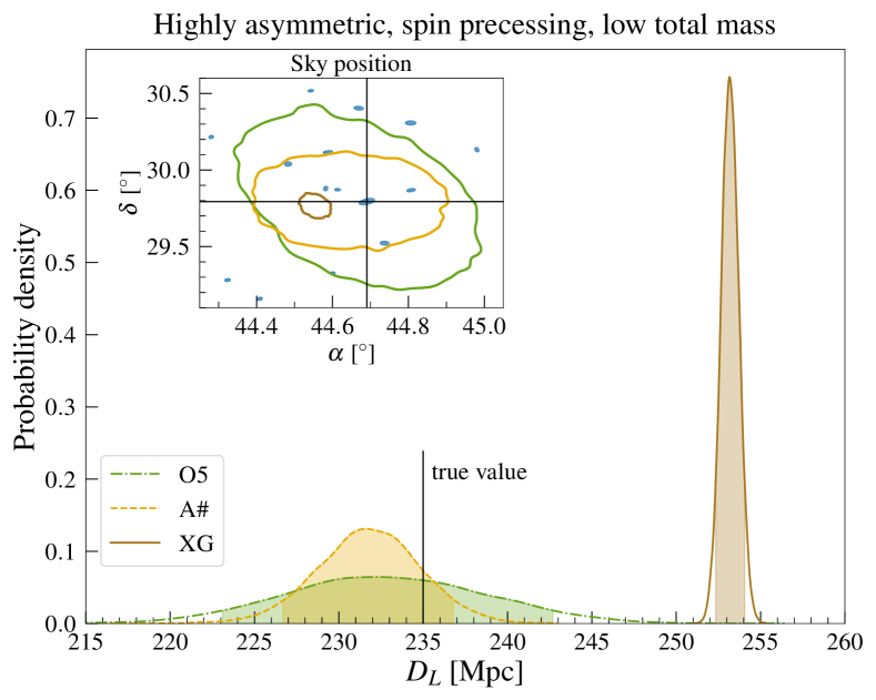
Figure 13: The distance posteriors for the Binary 1, Binary 2, and Binary 3 systems (from top to bottom) in the three detector networks considered in this study, The shaded region shows the 90% credible interval. The contours in the inset show the 90% credible region for the corresponding sky position measurement. The true values are denoted by black lines.

VI.3 Impact on science objectives

In the rest of the section, we investigate the effect of systematic bias on various science objectives. Even though we isolate different science objectives to discuss them individually, this is an artificial separation since the science is interconnected and so are the biases. Therefore, some of the same results may be discussed in different sections in slightly different ways. For instance, a biased measurement of the maximum NS mass has not only consequences for nuclear physics, but also for cosmology. Similarly, different representations of the same parameter space may be helpful in highlighting different aspects of the science. For instance, we refer to the magnitude and tilt of the spin vector when discussing lower mass-gap events, effective spin and spin-precession parameters when discussing astrophysical formation channels of heavy BBHs, and the relative orientations of the spin vectors when talking about spin morphologies. They are all different slices of the same spin space. However, the different parameterizations are useful for telling and highlighting different aspects of the full story.

VI.3.1 Cosmology

The luminosity distance and sky localization posteriors for the three simulated systems in the different detector networks are shown in Fig. 13. An illustration of an expected distribution of galaxies in a volume uncertainty region is depicted as blue ellipses. The volume uncertainty includes galaxies with redshift between $z_{\rm min}=H_{0,{\rm min}}/D_{L,{\rm max}}$ and $z_{\rm max}=H_{0,{\rm max}}/D_{L,{\rm min}}$, where $H_{0,{\rm min}}=35\rm\,km\,s^{-1}Mpc^{-1}$ and $H_{0,{\rm max}}=140\rm\,km\,s^{-1}Mpc^{-1}$, and $D_{L,{\rm min}}$ and $D_{L,{\rm max}}$ are the edges of the 90% credible interval of the $D_{L}$ posterior. The sky patch is the size of the inset panel that contains the sky location posterior. The areal density of luminous L* galaxies in the local Universe is taken to be $0.07\,\rm deg^{-2}$ at a distance of 100 Mpc [124].

While the localisation volume of the Binary 1 system (upper panel) is accurately measured for current detectors at design sensitivity and their next upgrade, both the distance and the sky position are biased for the XG network. With a sky position measurement precision of $<0.1\rm\,deg^{2}$ at 90% credibility, atmost a single galaxy is expected to be in a volumetric cone up to the distance to the event [36]. An inaccurate GW measurement will completely miss the host galaxy in this specific example or result in the identification of the wrong host in general. From Fig. 12, it is clear that such a system will give a biased distance estimate for sources at distances up to $\sim 35$ times farther, having an SNR $\gtrsim 30$ in the XG network.

For the Binary 2 system (middle panel), while O5 and A# networks accurately recover the sky position again, the distance is biased for all three networks. A bias in the distance measurement towards larger values will cause the $H_{0}$ measurement to be systematically biased towards smaller values. As in the case of the previous system, the precision in the sky position measurement for the XG network implies the existence of a single galaxy in the volume uncertainty region on average. Figure 12 tells us that the distance bias is important in O5 and A# networks for SNRs $\sim 70$ which implies distances of $\sim 800$ Mpc and $\sim 1300$ Mpc, respectively, while the distance at which $|\delta\vartheta/\Delta\vartheta|=1$ for the XG network is $\sim 5700$ Mpc. Even at a distance which is $\sim 7$ ($\sim 4$) times the maximum distances in O5 (A#), the event in XG will have an SNR of 130.

The measurement of both the distance and sky position is inaccurate for the Binary 3 system (lower panel) for all three detector networks under consideration. However, the distance bias, particularly for the XG network, is smaller than the previous systems. On the other hand, the sky position is biased even for O5 and A# networks. Due to the smaller distance biases, we see from Fig. 12 that the bias horizon for the XG network is also smaller resulting in a very loud signal of SNR $\sim 400$. Meanwhile, since the SNRs in the three detector networks for this system are smaller than the Binary 2 system, an SNR of $\sim 35$ in the O5 network is sufficient for a material distance bias.

Given that a two percent measurement of the Hubble constant will resolve the Hubble tension, all the three events in the XG network can single-handedly resolve the tension while the Binary 2 and the Binary 3 event can do so even in an A# network, at the simulated distance of $D_{L}=235\rm\,Mpc$.

VI.3.2 Lower mass gap

Figure 14: Corner plot showing the posterior distributions for the mass and dimensionless spin magnitude of the secondary companion of the Binary 1 system in the three detector networks in which the system is simulated. The shaded region in the 1D posteriors and the contours in the 2D space denote the 90% credible region. The black lines show the true injected value. A smaller minimum frequency for the XG network ($f_{\rm low}=5\rm\,Hz$) compared to the O5 and A# networks ($f_{\rm low}=10\rm\,Hz$) results in a smaller bias for the mass.

In Fig. 14, the recovered distributions for the mass and dimensionless spin magnitude of the secondary companion of the Binary 1 system in the three detector networks are shown. Since this is a highly asymmetric merger, the spin of the secondary is poorly measured as is clear from the $\chi_{2}$ posteriors in the O5 and A# networks. Nevertheless, the measurement precision improves significantly in the XG network, both due to its broad sensitivity improvement and a smaller minimum frequency. However, the measured value is materially inaccurate predicting a much lower value than the injection. This would affect inference on hierarchical formation channels and accretion-induced mass growth of a NS since both predict a large component spin. Instead, primordial BH formation scenarios that predict small spins would be favoured [176]. The measurement bias in the component mass would also have impacts on constraints on the speed-of-sound relation in NSs [168, 169] and inference on the effect of rotation on NS radii [173].

More directly, the upper edge in the mass distribution of astrophysical NSs can be used to determine the redshift and, thereby, estimate $H_{0}$ [154, 155, 156, 157]. Hence, an inaccurate determination of the edge of the mass distribution could also bias cosmological parameter estimation. This effect can be quantified using some simple calculations. Assume that the NS mass distribution is uniform and this system lies at the edge of that distribution. It can be shown that the error in the determination of the upper edge of the mass distribution is given by $\Delta m_{\rm max}={\rm max}\left[\sqrt{\sigma_{m}\,R_{o}/(N-1)},R_{o}/(N-1)\right]$, where $R_{o}=(m_{{\rm max},o}-m_{{\rm min},o})$, $\sigma_{m}$ is the typical mass measurement uncertainty for systems near the upper edge, $N$ is the number of observations and $m_{{\rm max},o}$ and $m_{{\rm min},o}$ are the maximum and minimum observed NS masses, respectively [220, 221]. The posterior peak of the secondary companion in A# network is $\sim 0.08M_{\odot}$ away from the true value. It is easy to calculate from the above equation that with $N\sim 20$ observations and $m_{\rm min}=1M_{\odot}$, the measurement error in determining the upper edge of the mass distribution is $\Delta m_{\rm max}\sim 0.08M_{\odot}$.

The merger rate of a Binary 1 binary within a distance of 235 Mpc is 1 every 3 years. Several studies have estimated that upcoming GW observing runs are expected to detect tens of BNS mergers per year [27, 32]. Therefore, a systematic bias in the mass and spin measurement can bias the inference of NS properties and cosmological parameters in the near future.

VI.3.3 PISN mass-gap

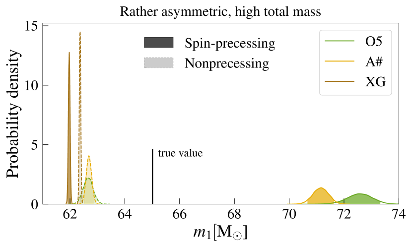
Figure 15: The posterior distributions of the primary mass for the Binary 2 (solid lines) and Binary 3 (dashed lines) systems in the three detector networks. The true injected value is shown by the vertical black line. The filled regions depict the 90% credible interval.

We report the measurements of the primary mass for the Binary 2 and Binary 3 systems in Fig. 15 in the three detector networks. While the biases in the aligned spin binary are less than in the precessing case, the measured values for both are significantly different from the injected value.

Furthermore, knowledge of the BH mass spectrum, particularly the edge of the mass distribution, can be used for cosmological inference as with the NS mass distribution. Following similar calculations and considering the simplified case where the BH mass distribution follows a power-law, $p(m)\propto m^{\alpha_{m}}$, with power-law index $\alpha_{m}=-3.5$ and sharp cutoffs at $m_{\rm min}=10M_{\odot}$ and $m_{\rm max}=65M_{\odot}$, it can be shown that the error in the determination of the upper cutoff is given by,

$$\Delta m_{\rm max}=\frac{(m_{{\rm max},o}^{\alpha_{m}+1}N-m_{{\rm min},o}^{\alpha_{m}+1})^{\frac{1}{\alpha_{m}+1}}}{(N-1)^{\frac{1}{\alpha_{m}+1}}}-m_{{\rm max},o},$$ (23)

until $\Delta m_{\rm max}\sim\sigma_{m}$, the individual event mass-measurement uncertainty. This uncertainty for $N=10^{3}$ events is then $\Delta m_{\rm max}\approx 3\,M_{\odot}$. From Fig. 15, it can be observed that the systematic error becomes dominant, even for the O5 network which is expected to observe $\mathcal{O}(10^{3})$ events every year.

VI.3.4 Spin morphology

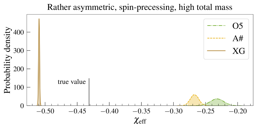
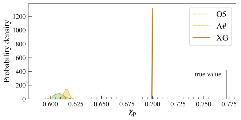
Figure 16: The posterior probability distribution of the $\chi_{\rm eff}$ (left) and $\chi_{\rm p}$ (right) parameters for the Binary 3 system in the three detector networks. The true value of the injection is shown by the black vertical line. The filled regions show the 90% credible interval.

In Fig. 16, the posterior distributions of $\chi_{\rm eff}$ and $\chi_{\rm p}$ are depicted for the Binary 3 system in the three detector networks. It is immediately clear that the posterior distributions for both spin parameters and in all three detector networks are far from the true value. However, it is also noticeable that the absolute value of the bias is larger for the current networks and their upgrades compared to the future XG network. Spin precession measurements are enabled by low-frequency sensitivity since the modulations in the GW amplitude due to spin precession occur on these timescales. Moreover, different waveform models agree to a greater degree at lower frequencies because this regime is closely informed by PN calculations in the various models. Therefore, a smaller minimum frequency and a better low-frequency sensitivity enable a more precise and accurate measurement of the $\chi_{\rm eff}$ and $\chi_{\rm p}$ parameters in the XG network. Even so, the parameters are significantly biased.

The posterior distributions of the parameters characterising the spin morphology for the Binary 1 and Binary 3 system are reported in Figs. 17 and 18. Let us analyze the Binary 1 system first. The tilt angles determine which morphology the binary falls into. It is observed that both the tilt angles are recovered inaccurately. While the median bias for $\theta_{2}$ is greater than that for $\theta_{1}$, with the median value of $\theta_{2}$ being $1.5-2$ times the injected value, the poor measurement accuracy due to the highly asymmetric and low total mass nature of the binary results in the median value of $\theta_{1}$ being farther away from the true value, when expressed as a multiple of sigma (the measurement error). The parameter $\phi_{12}$, which characterizes the spin morphology, is also heavily biased with the best-fit median values $2-3$ times the injected value depending on the detector network.

Now, considering the Binary 3 system, it is observed that the measurement accuracy increases due to the greater total mass and a resultant higher SNR. Similar to the Binary 1 system, the systematic bias in the $\theta_{1}$ is smaller in absolute terms compared to $\theta_{2}$, whose median inferred value is $0.4-0.6$ the injected value. Interestingly, $\phi_{12}$ is less biased for the O5 and A$\#$ networks. The estimates in the XG network are not only more biased but also completely different from the O5 and A$\#$ networks revealing the sensitivity of the measurement to the minimum frequency. Specifically, the measured value of $\phi_{12}$ in the XG network is consistent with $0^{\circ}$ while the injected value is around $200^{\circ}$.

Figure 17: The posterior distributions of the tilt angles, $\theta_{1}$ and $\theta_{2}$, and the relative in-plane spin angle, $\phi_{12}$, for the Binary 1 (left) and Binary 3 (right) systems. The black cross-hairs show the true injected value. For the Binary 1 system, on the left panel, the recovered distributions in all three networks are shown while for the Binary 3 system, on the right panel, those for the O5 and A$\#$ networks are reported. The probability distributions in the XG network are very different and are, therefore, presented in Fig. 18.

Figure 18: The posterior distributions of the tilt angles, $\theta_{1}$ and $\theta_{2}$, and the relative in-plane spin angle, $\phi_{12}$, for the Binary 3 system in the XG network. The black cross-hairs show the true injected value. The result for this case is shown separately from Fig. 17 because it is significantly different from the other networks and incorporating them in the same figure distorts its appearance.

VI.3.5 Remnant quantities

Figure 19: The final mass (left) and final spin (right) posteriors for the Binary 1, Binary 2, and Binary 3 systems (from top to bottom) in the three detector networks considered in this study. The true values are denoted by black lines.

We report the inferred remnant quantities for the Binary 1, Binary 2, and Binary 3 systems (top to bottom) in the three detector networks in Fig. 19. Unsurprisingly, there is significant bias in most of the cases. Since we reported the biases in various mass and spin quantities in the preceding sections, the biases in the remnant quantities are expected. It can also be observed from the figure that the remnant properties of high-mass systems are better measured compared to the low-mass system. Consequently, the biases for Binary 2 and Binary 3 as a multiple of the measurement error is larger.

VI.3.6 Maximal BH spin

Figure 20: The probability distributions of the secondary dimensionless spin magnitude $\chi_{2}$ in the Binary 2 (left) and Binary 3 (right) systems in the O5 and A$\#$ networks. The injected signal is generated using SEOBNRv5PHM while the template model is IMRPhenomXPHM. While the estimates are biased for both the systems and in both the detector networks, the more interesting feature is that the recovered $\chi_{2}$ distributions imply a maximally spinning secondary. We do not show the posterior in the XG network because they do not rail against the boundary, albeit still being biased.

In Fig. 20, the posterior distributions on the secondary dimensionless spin magnitude $\chi_{2}$ are reported for the Binary 2 (left panel) and Binary 3 (right panel) systems. It is observed that $\chi_{2}$ is biased for both systems. While the effect of $\chi_{2}$ on the GW waveform is subdominant due to the high mass asymmetry and smaller magnitude compared to $\chi_{1}$, which results in a poorer measurement of this parameter compared to $\chi_{1}$, the significantly biased recovery hints at systematic differences in the modeling of the effects of the parameter on the GW waveform. Perhaps, more interestingly, the secondary is measured to be maximally spinning. This is of huge importance because such a measurement in a real event would be revolutionary.

As shown in Fig. 10, the measurement of $\chi_{2}$ will be biased even for low SNR, albeit the prior will start becoming important at such SNRs.

VII Discussion and Conclusion

In this work we have studied systematic biases arising in state-of-the-art BBH waveform models used by the LVK Collaboration, in particular the quasi-circular, spin-precessing, multipolar IMRPhenomXPHM and SEOBNRv5PHM models. With increasing detector sensitivities of the current LVK network, its future upgrades, and XG detectors ahead, quantifying waveform systematics becomes central in achieving the promising science goals of GW astronomy. Unbiased parameter estimation is crucial for a range of applications, from individual events to the entire BBH population. Moreover, it is also vital for precision tests of GR as the prevailing theory of gravity.

Throughout this work, we have assumed that the true signal can be represented by SEOBNRv5PHM, and modeled it with IMRPhenomXPHM. Although both models do not represent exact solutions, using them in this way for injection-recovery studies allows one to explore a wide range of the BBH parameter space, for which accurate NR simulations are not yet available.

To quantify the bias in parameter estimation, we utilized statistical tools from LSA and full Bayesian analysis (see Sec. III). While LSA is approximate and relies on large-SNR events, it can forecast results for a large number of events, which is what we are interested in. Here, the two main methods are the FIM to approximate measurement errors and the bias formula to predict the systematic errors. The full Bayesian analysis is computationally expensive but more reliable, which makes it suitable for understanding selected events in detail. With these methods, we studied biases and performed hierarchical inference on the BBH population in Sec. IV. We explored vast parts of the BBH parameter space in Sec. V and investigated in detail the impact of systematics on the science cases of individual events in Sec. VI. In the following, we summarize our main results.

Our first result is mainly on the “use and abuse” of the widely used bias formula based on the LSA. By comparing with full Bayesian results, we explicitly demonstrated that the direct application of the bias formula without a “waveform alignment” procedure, as described in Eq. (12), can yield unreliable results. To our knowledge, this has not been discussed in the literature yet, and it is not explained in the main references for the bias formula [100, 119]. We find good agreement with full Bayesian results only after performing alignment and proper bookkeeping of the adjusted parameters. When not correcting for it, one would predict biases in the BBH population that could overestimate the actual bias by two orders of magnitude. This is particularly important when comparing waveforms of different families. Even after such caretaking, it is important to keep in mind that the LSA is an approximate estimate of the biases and statistical errors. We include discussions on the validity of the estimates and possible shortcomings of the method.

Regarding the LVK-like BBH population studied in Sec. IV, we find that the vast majority of events measured with the O5 and A$\#$ networks are not biased, around $2.5\%$ of the events, whereas, for XG detectors, up to $25\%$ of the events are expected to show biases. This is most clearly reported in Fig. 6, which relates the mismatch of each event with the ratio of systematic to statistical error. Although the bias relative to the statistical error is larger for XG detectors, the absolute bias per-se is smaller thanks to the detectors’ improvement at low frequencies, which allows to better observe the signal in the inspiral regime, where waveform models agree best. Thus, when combining all events through a hierarchical Bayesian analysis on the observed population, we find that the impact of systematic biases is more pronounced for A$\#$ than for XG detectors. As illustrated in Fig. 7, the most biased parameter is the magnitude of the spin of the primary, with the recovered distribution peaking at smaller values, while exhibiting a tail at large spin magnitudes that is absent in the injected population. The latter feature, in particular, could erroneously guide astrophysical formation scenarios into explaining the existence of a sizeable number of BHs with large spins. We stress that the bias estimates obtained with the LSA might be overly pessimistic, since it relies on the quadratic approximation to the likelihood, which holds only in the high SNR regime. Thus, the impact on the population might be exaggerated for O5 and A$\#$ networks, but we expect our results for XG to be more accurate.

When spanning the possible BBH parameter space in Sec. V, we sampled events with uniform distribution $\chi_{\text{p}}\in[0,1]$, uniform in total detector-frame mass $\in[10,200]\,M_{\odot}$ and uniform in inverse mass ratio $1/q\in[1,30]$. Although this does not represent the LVK BBH population, exploring the challenging parts of the parameter space is important, since GW events in these regions may be discovered with future more sensitive detectors. Using the LSA, we computed for each parameter the bias horizon, which describes the maximum distance up to which an event is systematically biased, after which the SNR is low enough that the statistical error is larger than the systematic one. Since most of these binaries are difficult to model, analytically and numerically, not surprisingly the biases are more important than for the LVK-like population of Sec. IV.

Furthermore, our detailed analysis of selected events summarized in Table 1 in Sec. VI has several important findings depending on the science cases.

Focusing on cosmological implications in Sec. VI.3.1, we find that distances and sky localization can be significantly biased. Here, one would be unable to infer the correct value of the Hubble-Lemaître parameter and thus not resolve the Hubble-Lemaître tension. Biases in the sky position can be sufficiently large to prevent the correct identification of the host galaxy. This would be drastic, since single XG events have the potential to determine $H_{0}$ to few percent. Furthermore, those biases may also affect the determination of $H_{0}$ from stacking GW events, requiring a dedicated future study.

When studying the lower mass gap in Sec. VI.3.2, we report that the estimate of the secondary mass for the highly asymmetric, spin-precessing low total-mass system would be underestimated in all networks. The spin of the secondary would be significantly underestimated in the XG network. This could lead to wrong estimates of the upper edge of the NS mass distribution, which would inflict further biases for studies of the equation of state and again $H_{0}$. The PISN mass-gap is investigated in Sec. VI.3.3. Here we show that the estimate of the upper mass-gap through the primary mass by the high total-mass binaries is strongly biased even for O5. Although precession changes the primary mass posteriors of both binaries significantly, the injected value for $m_{1}$ is not recovered within the $90\,\%$ credible for any network.

In Sec. VI.3.4 we look into the spin morphology, and find that XG detectors are not always more prone to biases than O5 and A#. By extending the detectors’ bandwidth to lower frequency where the waveform models are more similar, the recovery of spin parameters can become closer to the injected values, at least for the low total-mass system. The remnant quantities are studied in Sec. VI.3.5, where we report the final mass and final spin of the remnant for all three “golden” binaries. Both upper mass-gap events have significant measurement bias excluding the injected values far outside the $90\,\%$ credible interval. For the highly asymmetric and precessing binary with low total mass, the overall biases are not as strong, but besides the final spin in O5 also outside the $90\,\%$ credible interval. By performing an independent ringdown analysis, at least for XG, one may conclude violations from the Kerr hypothesis and thus violations from GR (not done in this work).

In Sec. VI.3.6 we observed that the two high total-mass events predict posteriors for $\chi_{2}$ that rail against the maximum spin of a BH for O5 and A#. If not identified as systematic bias, this would certainly have important consequences for astrophysical formation channels in explaining such high spins in BBH systems, as well as theoretical interest in extremal Kerr BHs and eventually exotic compact objects.

In summary, depending on the binary’s parameters, biases can be present for the upcoming LVK O5 run and can affect crucial science. As expected, systematics become even more relevant with increasing detector sensitivity and thus they are important for future XG detectors. The fact that many exciting science cases can be jeopardized by biases underlines the importance of improving existing waveform models. It also motivates the need to include modeling error estimates when performing parameter estimation, even if this will inevitably broaden our posteriors. Lastly, much more work would be needed to quantify more robustly the waveform systematics — for example by employing as signals NR and NRSur waveforms, where available, and extending the current study to binaries on generic orbits, notably BBHs on eccentric orbits.

The main limitation of our work in the use of the LSA for the population analysis. While it is the most readily available and feasible way to conduct a study like ours, one can be critical about its validity across the parameter space and view the ensuing conclusions with a grain of salt. In the future, we intend to do population-scale studies using modern data analysis tools, such as DINGO [222], that allow for rapid evaluations of the posteriors.

Note: While working on this paper, we became aware of a complementary study, Ref. [223], that focuses on assessing waveform systematics for XG detectors using two quasi-circular aligned-spin models.

Appendix A Toy model

We consider a simple toy model to illustrate the effect of nonuniform parameter definitions across waveform models on the systematic bias calculated under LSA using Eq. (11). For this example, we take the IMRPhenomXPHM model as both the signal and the template. However, we shift the signal by $\tau$, evaluating it at $t_{c}=\tau$, while the template is evaluated at $t_{c}=0$. Note that for a pair of arbitrary waveform models, we do not know of the shift $\tau$ a priori and, thence, compute the bias at $t_{c}=0$. In a Bayesian analysis, this would simply mean that the likelihood distribution for $t_{c}$ peaks at $t_{c}=\tau$, for a noiseless injection, without impacting any physical paraemeter.

Let us now examine how the predictions of the bias formula Eq. (11). We consider a reduced two dimensional parameter space, $\bm{\vartheta}=\{D_{L},t_{c}\}$. Here, the bias for the two parameters can be calculated analytically. The distance bias is given by

$$\delta D_{L} =\frac{D_{L}^{2}}{\left<h|h\right>}\left<-h/D_{L}|h(t_{c}=\tau)-h(t_{c}=0)\right>$$ (24)

$$=\frac{D_{L}^{2}}{\left<h|h\right>}\left<-h/D_{L}|h(t_{c}=0)e^{-2\pi if\tau}-h(t_{c}=0)\right>$$

$$=0+\mathcal{O}(\tau^{2}),$$

while the $t_{c}$ bias reduces to

$$\delta t_{c} =\frac{1}{\left<2\pi ifh|2\pi ifh\right>}\left<-2\pi ifh|h(t_{c}=\tau)-h(t_{c}=0)\right>$$ (25)

$$=\frac{-2\pi}{\left<2\pi ifh|2\pi ifh\right>}\left<ifh|h(t_{c}=0)e^{-2\pi if\tau}-h(t_{c}=0)\right>$$

$$=\tau+\mathcal{O}(\tau^{2}).$$

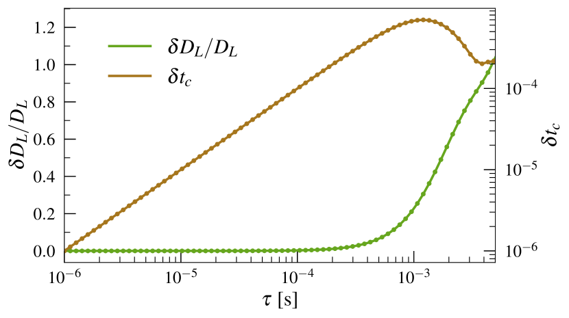
Figure 21: The bias in the luminosity distance and time of coalescence parameters as a function of a time shift in the signal for the simple toy model considered in Sec. A. For very small values of the time shift parameter $\tau$, the estimates of the bias formula are reliable but it starts deviating for $\tau$ values which are still small.

In Fig. 21, we show the bias in the luminosity distance and time of coalescence calculated using Eq. (11). We see that the estimates get contributions from the quadratic and higher order terms of Eq. (24) and Eq. (25) for small values of the time shift $\tau$. However, these corrections are not physical since $D_{L}$ should not be biased for simple time shifts of the signal and the bias in $t_{c}$ should simply correspond to the value of the time shift. While the incorrect estimates for the $t_{c}$ bias is not of physical consequence in most cases, it is readily seen from the figure that the $D_{L}$ bias can be incorrectly estimated to very large values impacting the outlook on science applications like cosmology where the $D_{L}$ parameter is crucial.

Appendix B Effect of $f_{\rm low}$ for higher modes in SEOBNRv5PHM signal

Figure 22: The posterior distributions of select parameters for the Binary 1 system in O5 network with different minimum frequencies at which the SEOBNRv5PHM signal is generated. The starting frequency for the analysis is 10 Hz for both cases. The indistinguishability of the distributions in the two cases shows that the absence of certain subdominant harmonics in the signal at low frequencies for the case depicted in green is inconsequential to the analysis.

When generating an SEOBNRv5PHM waveform, the minimum frequency refers to the frequency of the $(l,m)=(2,2)$ harmonic. Higher harmonics in the given time segment occur at a higher frequency. This is a feature of all time-domain waveforms. Since phenomenological waveforms are constructed in the frequency domain, all the harmonics are present at any given frequency. This means that in analysing a GW signal generated using SEOBNRv5PHM with IMRPhenomXPHM (with the same minimum frequency), the template contains the higher harmonics at frequencies lower than where the same is present in the signal. For instance, if $f_{\rm low}=10\rm\,Hz$ for both SEOBNRv5PHM and IMRPhenomXPHM, the $(l,m)=(3,3),(4,4)$ harmonics for the SEOBNRv5PHM signal start at $15\rm\,Hz$ and $20\rm\,Hz$, respectively.

All analyses in the paper are done by taking the same $f_{\rm low}$ for both SEOBNRv5PHM and IMRPhenomXPHM waveforms. We verify in Fig. 22 that this does not affect any of the results of the paper. The figure shows the posterior distributions of select parameters of the Binary 1 system for two cases simulated in the O5 network. For the distributions plotted in orange, the SEOBNRv5PHM waveform is generated starting $f_{\rm low}=5\rm\,Hz$ while the analysis is done using IMRPhenomXPHM setting $f_{\rm low}=10\rm\,Hz$. On the other hand, the SEOBNRv5PHM waveform is generated with $f_{\rm low}=10\rm\,Hz$ for the case in green and an identical analysis setting as the previous case. We remark that the posterior distributions in the two cases are indistinguishable.

Appendix C Effect of $f_{\rm low}$ on parameter estimation and bias

Figure 23: The posterior distributions in the $\mathcal{M}_{c}-\chi_{\rm eff}$ parameter space for the Binary 1 system in O5 network is shown with different minimum frequency, $f_{\rm low}$, are shown. Note that a smaller minimum frequency results in a greater measurement precision and a smaller bias.

We briefly discuss the impact of the minimum frequency $f_{\rm low}$ used in analyzing a GW signal. This is of particular importance given the excess low frequency noise in the Advanced LIGO and Advanced Virgo detectors limiting the low frequency cut-off to 20 Hz instead of the predicted 10 Hz.

We generate a signal corresponding to the Binary 1 system in the O5 network at two starting frequencies $f_{\rm low}=10,20\rm\,Hz$ with the SEOBNRv5PHM model. This signal is then analyzed with the respective starting frequencies used in its generation with the IMRPhenomXPHM model as the template. The posterior distributions in the $\mathcal{M}_{c}-\chi_{\rm eff}$ parameter space are reported in Fig. 23. The distributions on the other non-derivative parameters are not reported since they are similar in both cases. It is observed that a lower minimum frequency leads to a smaller measurement error and bias for the chirp mass. Since $\chi_{\rm eff}$ has a large (positive) correlation with $\mathcal{M}_{c}$, as seen from the figure, it is also affected in a similar manner.

The number of cycles in a GW waveform is inversely related to the minimum frequency and $\mathcal{M}_{c}$ is the leading order contributor to this. Hence the large number of GW cycles between 10 Hz and 20 Hz leads to a better measurement precision for $\mathcal{M}_{c}$. This is also the part of the waveform where different models are in better agreement since all models have to reproduce the PN limit leading to a more accurate measurement. This is precisely why the absolute magnitude of the $\mathcal{M}_{c}$ bias in the XG network, which has $f_{\rm low}=5\rm\,Hz$, is smaller than the O5 and A# networks.

Appendix D Dependence of $|\delta\vartheta/\Delta\vartheta|$ on the SNR

Figure 24: The ratio between the systematic bias and statistical errors for select parameters as a function of the SNR for a population of BBH mergers as observed by the LVK. A network SNR threshold of 12 was imposed on the $10^{5}$ binaries in the population resulting in $\sim 1800$ and $\sim 8100$ in the O5 (top) and A# (bottom) networks respectively. The colorbar depicts the mismatch between SEOBNRv5PHM and IMRPhenomXPHM waveform models.

In the following, we report complementary results for the same data as presented in Fig. 6. Fig. 24 shows how the ratio $|\delta\vartheta/\Delta\vartheta|$ depends on the SNR (instead of the mismatch) and the colorbar now indicates the mismatch. The panels are structured similarly to those of Fig. 6. Overall, the cumulation of biased events (ratio larger than one) depends strongly on the mismatch, although outliers exist for all networks. In all cases, the number of events with a ratio much smaller than one decreases as a function of the SNR, although strongly biased events do exist even for small SNRs. These results underline the importance of improving waveform modeling to reduce mismatches for all detector networks, not only for XG.

Appendix E Distribution of population parameters

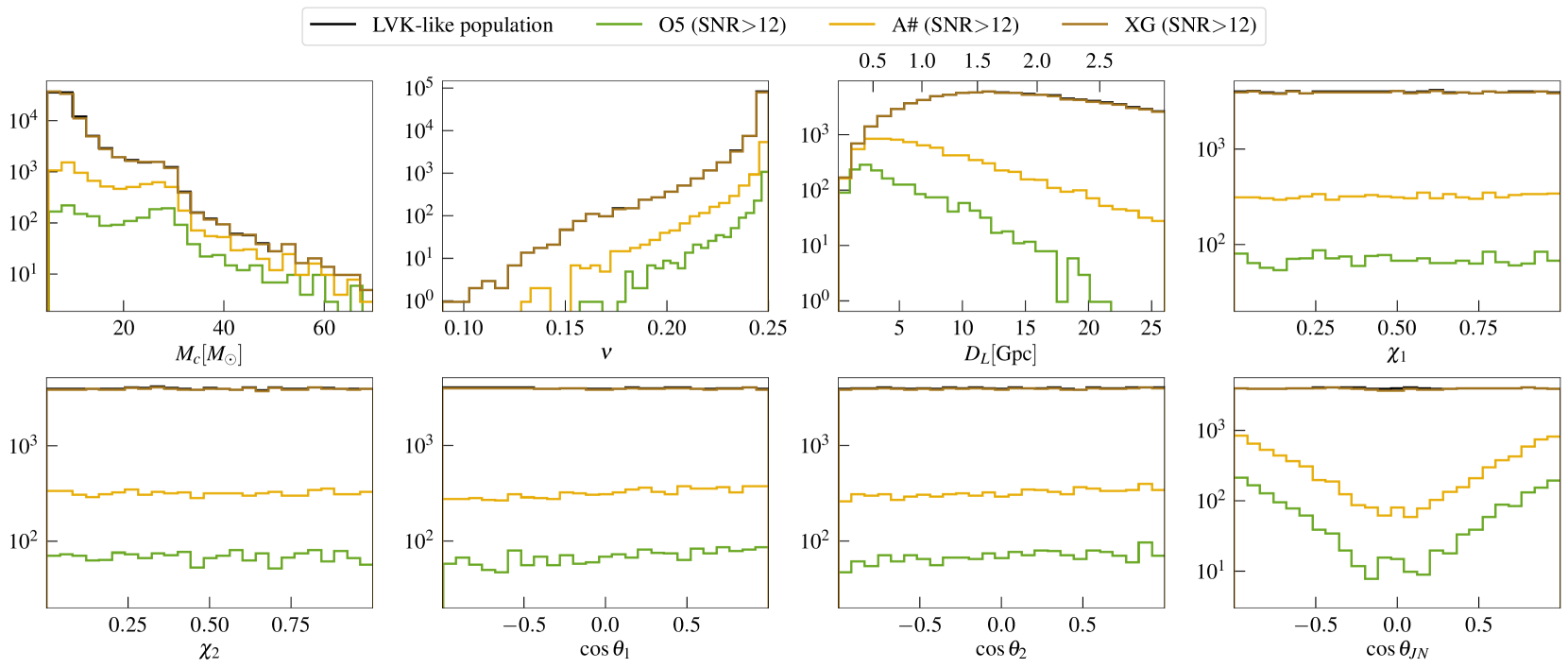
Figure 25: The distribution of select parameters of the LVK-like BBH population and of the detectable population in the three detector networks. The black line overlaps almost entirely with the detectable population in the XG network.

In the panels of Fig. 25, we show the distribution of parameters of detectable events from the LVK-like BBH population for the different networks. The detectability criterion is SNR$>12$, which acts as a strong filter for O5 and A#, but only very mildly impacts XG. The parameters $a_{1},a_{2},\cos\theta_{1},\cos\theta_{2}$ are distributed uniformly for all networks, which agrees well with the population. However, the shape of the distributions describing the parameters $M_{c},\nu,D_{L},\cos\theta_{\text{JN}}$ is more complicated and changes throughout the networks. This implies a significant selection bias unless one uses XG. Note that $\cos\theta_{\text{JN}}$ is sampled from a uniform distribution but shows strong selection bias for O5 and A#.

Appendix F Bias in $\chi_{1}$ when scanning the parameter space

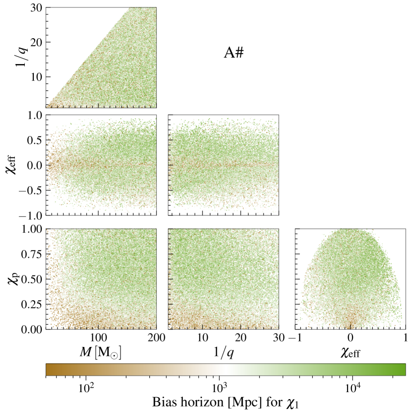
Figure 26: The scatter shows the distribution of the 50,000 binaries in the parameter space represented in Fig. 9, while the color scale shows the distance to which the $\chi_{1}$ parameter is biased ($\delta\chi_{1}/\Delta\chi_{1}\geq 1$) for the O5 (left) and A# (right) networks. Systematic biases become less important if a binary is at a larger distance since measurement precision decreases with distance. Therefore, a large bias horizon signifies that a given parameter ($\chi_{1}$ in this case) is measured well enough for systematic biases to be important even at such large distances. Notice that the binaries are biased up to a greater distance in the A# network compared to the O5 network due its greater sensitivity, and the resultant improvement in measurement precision.

Figure 27: Same as Fig. 26 for the XG network. BBHs observed with the XG network are biased up to a greater distance than those observed with either the O5 or A# networks, due its greater sensitivity, and the resultant improvement in measurement precision, with a majority of the binaries having a bias horizon $\geq 25\,\rm Gpc$ ($z\approx 3$) beyond which stellar-origin BBHs are not expected to exist.

In Fig. 26 and Fig. 27, we show the bias horizon for the parameter $\chi_{1}$. The binaries are distributed as described in Sec. V.

References

- Abbott et al. [2016a] B. P. Abbott et al. (LIGO Scientific, Virgo), Phys. Rev. Lett. 116, 061102 (2016a), arXiv:1602.03837 [gr-qc] .
- Aasi et al. [2015] J. Aasi et al. (LIGO Scientific), Class. Quant. Grav. 32, 074001 (2015), arXiv:1411.4547 [gr-qc] .
- Acernese et al. [2015] F. Acernese et al. (VIRGO), Class. Quant. Grav. 32, 024001 (2015), arXiv:1408.3978 [gr-qc] .
- Akutsu et al. [2021] T. Akutsu et al. (KAGRA), PTEP 2021, 05A101 (2021), arXiv:2005.05574 [physics.ins-det] .
- Abbott et al. [2021a] R. Abbott et al. (LIGO Scientific, VIRGO, KAGRA), (2021a), arXiv:2111.03606 [gr-qc] .
- Abbott et al. [2021b] R. Abbott et al. (LIGO Scientific, VIRGO), (2021b), arXiv:2108.01045 [gr-qc] .
- LIG [2024] (2024), arXiv:2404.04248 [astro-ph.HE] .
- Venumadhav et al. [2019] T. Venumadhav, B. Zackay, J. Roulet, L. Dai, and M. Zaldarriaga, Phys. Rev. D 100, 023011 (2019), arXiv:1902.10341 [astro-ph.IM] .
- Venumadhav et al. [2020] T. Venumadhav, B. Zackay, J. Roulet, L. Dai, and M. Zaldarriaga, Phys. Rev. D 101, 083030 (2020), arXiv:1904.07214 [astro-ph.HE] .
- Zackay et al. [2021] B. Zackay, L. Dai, T. Venumadhav, J. Roulet, and M. Zaldarriaga, Phys. Rev. D 104, 063030 (2021), arXiv:1910.09528 [astro-ph.HE] .
- Olsen et al. [2022] S. Olsen, T. Venumadhav, J. Mushkin, J. Roulet, B. Zackay, and M. Zaldarriaga, Phys. Rev. D 106, 043009 (2022), arXiv:2201.02252 [astro-ph.HE] .
- Mehta et al. [2023a] A. K. Mehta, S. Olsen, D. Wadekar, J. Roulet, T. Venumadhav, J. Mushkin, B. Zackay, and M. Zaldarriaga, (2023a), arXiv:2311.06061 [gr-qc] .
- Wadekar et al. [2023] D. Wadekar, J. Roulet, T. Venumadhav, A. K. Mehta, B. Zackay, J. Mushkin, S. Olsen, and M. Zaldarriaga, (2023), arXiv:2312.06631 [gr-qc] .
- Abbott et al. [2023a] R. Abbott et al. (KAGRA, VIRGO, LIGO Scientific), Phys. Rev. X 13, 011048 (2023a), arXiv:2111.03634 [astro-ph.HE] .
- Fishbach et al. [2018] M. Fishbach, D. E. Holz, and W. M. Farr, Astrophys. J. Lett. 863, L41 (2018), arXiv:1805.10270 [astro-ph.HE] .
- Abbott et al. [2018a] B. P. Abbott et al. (LIGO Scientific, Virgo), Phys. Rev. Lett. 121, 161101 (2018a), arXiv:1805.11581 [gr-qc] .
- Radice et al. [2018] D. Radice, A. Perego, F. Zappa, and S. Bernuzzi, Astrophys. J. Lett. 852, L29 (2018), arXiv:1711.03647 [astro-ph.HE] .
- De et al. [2018] S. De, D. Finstad, J. M. Lattimer, D. A. Brown, E. Berger, and C. M. Biwer, Phys. Rev. Lett. 121, 091102 (2018), [Erratum: Phys.Rev.Lett. 121, 259902 (2018)], arXiv:1804.08583 [astro-ph.HE] .
- Abbott et al. [2017a] B. P. Abbott et al. (LIGO Scientific, Virgo, 1M2H, Dark Energy Camera GW-E, DES, DLT40, Las Cumbres Observatory, VINROUGE, MASTER), Nature 551, 85 (2017a), arXiv:1710.05835 [astro-ph.CO] .
- Abbott et al. [2023b] R. Abbott et al. (LIGO Scientific, Virgo, KAGRA), Astrophys. J. 949, 76 (2023b), arXiv:2111.03604 [astro-ph.CO] .
- Abbott et al. [2016b] B. P. Abbott et al. (LIGO Scientific, Virgo), Phys. Rev. Lett. 116, 221101 (2016b), [Erratum: Phys.Rev.Lett. 121, 129902 (2018)], arXiv:1602.03841 [gr-qc] .
- Abbott et al. [2021c] R. Abbott et al. (LIGO Scientific, Virgo), Phys. Rev. D 103, 122002 (2021c), arXiv:2010.14529 [gr-qc] .
- Abbott et al. [2021d] R. Abbott et al. (LIGO Scientific, VIRGO, KAGRA), (2021d), arXiv:2112.06861 [gr-qc] .
- Punturo et al. [2010] M. Punturo et al., Class. Quant. Grav. 27, 194002 (2010).
- Maggiore et al. [2020] M. Maggiore et al., JCAP 03, 050 (2020), arXiv:1912.02622 [astro-ph.CO] .
- Reitze et al. [2019] D. Reitze et al., Bull. Am. Astron. Soc. 51, 035 (2019), arXiv:1907.04833 [astro-ph.IM] .
- Borhanian and Sathyaprakash [2022] S. Borhanian and B. S. Sathyaprakash, (2022), arXiv:2202.11048 [gr-qc] .
- Evans et al. [2021] M. Evans et al., (2021), arXiv:2109.09882 [astro-ph.IM] .
- Gupta et al. [2023] I. Gupta et al., (2023), arXiv:2307.10421 [gr-qc] .
- Branchesi et al. [2023] M. Branchesi et al., JCAP 07, 068 (2023), arXiv:2303.15923 [gr-qc] .
- Bogdanov et al. [2022] S. Bogdanov et al., in Snowmass 2021 (2022) arXiv:2209.07412 [astro-ph.HE] .
- Iacovelli et al. [2022] F. Iacovelli, M. Mancarella, S. Foffa, and M. Maggiore, Astrophys. J. 941, 208 (2022), arXiv:2207.02771 [gr-qc] .
- Woosley and Heger [2021] S. E. Woosley and A. Heger, Astrophys. J. Lett. 912, L31 (2021), arXiv:2103.07933 [astro-ph.SR] .
- Belczynski et al. [2016] K. Belczynski et al., Astron. Astrophys. 594, A97 (2016), arXiv:1607.03116 [astro-ph.HE] .
- Farmer et al. [2020] R. Farmer, M. Renzo, S. de Mink, M. Fishbach, and S. Justham, Astrophys. J. Lett. 902, L36 (2020), arXiv:2006.06678 [astro-ph.HE] .
- Borhanian et al. [2020] S. Borhanian, A. Dhani, A. Gupta, K. G. Arun, and B. S. Sathyaprakash, Astrophys. J. Lett. 905, L28 (2020), arXiv:2007.02883 [astro-ph.CO] .
- Pang et al. [2018] P. T. H. Pang, J. Calderón Bustillo, Y. Wang, and T. G. F. Li, Phys. Rev. D 98, 024019 (2018), arXiv:1802.03306 [gr-qc] .
- Maggio et al. [2023] E. Maggio, H. O. Silva, A. Buonanno, and A. Ghosh, Phys. Rev. D 108, 024043 (2023), arXiv:2212.09655 [gr-qc] .
- Hu and Veitch [2023] Q. Hu and J. Veitch, Astrophys. J. 945, 103 (2023), arXiv:2210.04769 [gr-qc] .
- Toubiana et al. [2023a] A. Toubiana, L. Pompili, A. Buonanno, J. R. Gair, and M. L. Katz, (2023a), arXiv:2307.15086 [gr-qc] .
- Bhat et al. [2023] S. A. Bhat, P. Saini, M. Favata, and K. G. Arun, Phys. Rev. D 107, 024009 (2023), arXiv:2207.13761 [gr-qc] .
- Saini et al. [2023] P. Saini, S. A. Bhat, M. Favata, and K. G. Arun, (2023), arXiv:2311.08033 [gr-qc] .
- Narayan et al. [2023] P. Narayan, N. K. Johnson-McDaniel, and A. Gupta, Phys. Rev. D 108, 064003 (2023), arXiv:2306.04068 [gr-qc] .
- Buonanno and Damour [1999] A. Buonanno and T. Damour, Phys. Rev. D 59, 084006 (1999), arXiv:gr-qc/9811091 .
- Buonanno and Damour [2000] A. Buonanno and T. Damour, Phys. Rev. D 62, 064015 (2000), arXiv:gr-qc/0001013 .
- Damour et al. [2000] T. Damour, P. Jaranowski, and G. Schaefer, Phys. Rev. D 62, 084011 (2000), arXiv:gr-qc/0005034 .
- Damour [2001] T. Damour, Phys. Rev. D 64, 124013 (2001), arXiv:gr-qc/0103018 .
- Buonanno et al. [2006] A. Buonanno, Y. Chen, and T. Damour, Phys. Rev. D 74, 104005 (2006), arXiv:gr-qc/0508067 .
- Ramos-Buades et al. [2022] A. Ramos-Buades, A. Buonanno, M. Khalil, and S. Ossokine, Phys. Rev. D 105, 044035 (2022), arXiv:2112.06952 [gr-qc] .
- Pompili et al. [2023] L. Pompili et al., Phys. Rev. D 108, 124035 (2023), arXiv:2303.18039 [gr-qc] .
- Ramos-Buades et al. [2023] A. Ramos-Buades, A. Buonanno, H. Estellés, M. Khalil, D. P. Mihaylov, S. Ossokine, L. Pompili, and M. Shiferaw, Phys. Rev. D 108, 124037 (2023), arXiv:2303.18046 [gr-qc] .
- van de Meent et al. [2023] M. van de Meent, A. Buonanno, D. P. Mihaylov, S. Ossokine, L. Pompili, N. Warburton, A. Pound, B. Wardell, L. Durkan, and J. Miller, Phys. Rev. D 108, 124038 (2023), arXiv:2303.18026 [gr-qc] .
- Khalil et al. [2023] M. Khalil, A. Buonanno, H. Estelles, D. P. Mihaylov, S. Ossokine, L. Pompili, and A. Ramos-Buades, Phys. Rev. D 108, 124036 (2023), arXiv:2303.18143 [gr-qc] .
- Nagar et al. [2018] A. Nagar et al., Phys. Rev. D 98, 104052 (2018), arXiv:1806.01772 [gr-qc] .
- Nagar et al. [2020a] A. Nagar, G. Pratten, G. Riemenschneider, and R. Gamba, Phys. Rev. D 101, 024041 (2020a), arXiv:1904.09550 [gr-qc] .
- Nagar et al. [2020b] A. Nagar, G. Riemenschneider, G. Pratten, P. Rettegno, and F. Messina, Phys. Rev. D 102, 024077 (2020b), arXiv:2001.09082 [gr-qc] .
- Gamba et al. [2022] R. Gamba, S. Akçay, S. Bernuzzi, and J. Williams, Phys. Rev. D 106, 024020 (2022), arXiv:2111.03675 [gr-qc] .
- Nagar et al. [2023] A. Nagar, P. Rettegno, R. Gamba, S. Albanesi, A. Albertini, and S. Bernuzzi, Phys. Rev. D 108, 124018 (2023), arXiv:2304.09662 [gr-qc] .
- Pretorius [2005] F. Pretorius, Phys. Rev. Lett. 95, 121101 (2005), arXiv:gr-qc/0507014 .
- Campanelli et al. [2006] M. Campanelli, C. O. Lousto, P. Marronetti, and Y. Zlochower, Phys. Rev. Lett. 96, 111101 (2006), arXiv:gr-qc/0511048 .
- Baker et al. [2006] J. G. Baker, J. Centrella, D.-I. Choi, M. Koppitz, and J. van Meter, Phys. Rev. Lett. 96, 111102 (2006), arXiv:gr-qc/0511103 .
- Pan et al. [2008] Y. Pan, A. Buonanno, J. G. Baker, J. Centrella, B. J. Kelly, S. T. McWilliams, F. Pretorius, and J. R. van Meter, Phys. Rev. D 77, 024014 (2008), arXiv:0704.1964 [gr-qc] .
- Ajith et al. [2007] P. Ajith et al., Class. Quant. Grav. 24, S689 (2007), arXiv:0704.3764 [gr-qc] .
- Hannam et al. [2014] M. Hannam, P. Schmidt, A. Bohé, L. Haegel, S. Husa, F. Ohme, G. Pratten, and M. Pürrer, Phys. Rev. Lett. 113, 151101 (2014), arXiv:1308.3271 [gr-qc] .
- Pratten et al. [2021] G. Pratten et al., Phys. Rev. D 103, 104056 (2021), arXiv:2004.06503 [gr-qc] .
- Estellés et al. [2022] H. Estellés, M. Colleoni, C. García-Quirós, S. Husa, D. Keitel, M. Mateu-Lucena, M. d. L. Planas, and A. Ramos-Buades, Phys. Rev. D 105, 084040 (2022), arXiv:2105.05872 [gr-qc] .
- Thompson et al. [2023] J. E. Thompson, E. Hamilton, L. London, S. Ghosh, P. Kolitsidou, C. Hoy, and M. Hannam, (2023), arXiv:2312.10025 [gr-qc] .
- Hannam et al. [2009] M. Hannam et al., Phys. Rev. D 79, 084025 (2009), arXiv:0901.2437 [gr-qc] .
- Hinder et al. [2014] I. Hinder et al., Class. Quant. Grav. 31, 025012 (2014), arXiv:1307.5307 [gr-qc] .
- Boyle et al. [2019] M. Boyle et al., Class. Quant. Grav. 36, 195006 (2019), arXiv:1904.04831 [gr-qc] .
- Rinne et al. [2009] O. Rinne, L. T. Buchman, M. A. Scheel, and H. P. Pfeiffer, Class. Quant. Grav. 26, 075009 (2009), arXiv:0811.3593 [gr-qc] .
- Buchman et al. [2012] L. T. Buchman, H. P. Pfeiffer, M. A. Scheel, and B. Szilagyi, Phys. Rev. D 86, 084033 (2012), arXiv:1206.3015 [gr-qc] .
- Buchman et al. [2024] L. T. Buchman, M. D. Duez, M. Morales, M. A. Scheel, T. M. Kostersitz, and A. M. Evans, (2024), arXiv:2402.12544 [gr-qc] .
- Chu et al. [2016] T. Chu, H. Fong, P. Kumar, H. P. Pfeiffer, M. Boyle, D. A. Hemberger, L. E. Kidder, M. A. Scheel, and B. Szilagyi, Class. Quant. Grav. 33, 165001 (2016), arXiv:1512.06800 [gr-qc] .
- Mitman et al. [2021] K. Mitman et al., Phys. Rev. D 103, 024031 (2021), arXiv:2011.01309 [gr-qc] .
- Blackman et al. [2015] J. Blackman, S. E. Field, C. R. Galley, B. Szilágyi, M. A. Scheel, M. Tiglio, and D. A. Hemberger, Phys. Rev. Lett. 115, 121102 (2015), arXiv:1502.07758 [gr-qc] .
- Varma et al. [2019a] V. Varma, S. E. Field, M. A. Scheel, J. Blackman, L. E. Kidder, and H. P. Pfeiffer, Phys. Rev. D 99, 064045 (2019a), arXiv:1812.07865 [gr-qc] .
- Varma et al. [2019b] V. Varma, S. E. Field, M. A. Scheel, J. Blackman, D. Gerosa, L. C. Stein, L. E. Kidder, and H. P. Pfeiffer, Phys. Rev. Research. 1, 033015 (2019b), arXiv:1905.09300 [gr-qc] .
- Yoo et al. [2023] J. Yoo et al., Phys. Rev. D 108, 064027 (2023), arXiv:2306.03148 [gr-qc] .
- Abbott et al. [2017b] B. P. Abbott et al. (LIGO Scientific, Virgo), Class. Quant. Grav. 34, 104002 (2017b), arXiv:1611.07531 [gr-qc] .
- Pürrer and Haster [2020] M. Pürrer and C.-J. Haster, Phys. Rev. Res. 2, 023151 (2020), arXiv:1912.10055 [gr-qc] .
- Hu and Veitch [2022] Q. Hu and J. Veitch, Phys. Rev. D 106, 044042 (2022), arXiv:2205.08448 [gr-qc] .
- Islam et al. [2023] T. Islam, A. Vajpeyi, F. H. Shaik, C.-J. Haster, V. Varma, S. E. Field, J. Lange, R. O’Shaughnessy, and R. Smith, “Analysis of GWTC-3 with fully precessing numerical relativity surrogate models,” (2023), arXiv:2309.14473 [gr-qc] .
- Puecher et al. [2024] A. Puecher, A. Samajdar, G. Ashton, C. Van Den Broeck, and T. Dietrich, Phys. Rev. D 109, 023019 (2024), arXiv:2310.03555 [gr-qc] .
- Jan et al. [2020] A. Z. Jan, A. B. Yelikar, J. Lange, and R. O’Shaughnessy, Phys. Rev. D 102, 124069 (2020), arXiv:2011.03571 [gr-qc] .
- Read [2023] J. S. Read, Class. Quant. Grav. 40, 135002 (2023), arXiv:2301.06630 [gr-qc] .
- Owen et al. [2023] C. B. Owen, C.-J. Haster, S. Perkins, N. J. Cornish, and N. Yunes, Phys. Rev. D 108, 044018 (2023), arXiv:2301.11941 [gr-qc] .
- Varma et al. [2014] V. Varma, P. Ajith, S. Husa, J. C. Bustillo, M. Hannam, and M. Pürrer, Phys. Rev. D 90, 124004 (2014), arXiv:1409.2349 [gr-qc] .
- Varma and Ajith [2017] V. Varma and P. Ajith, Phys. Rev. D 96, 124024 (2017), arXiv:1612.05608 [gr-qc] .
- Singh et al. [2023] M. K. Singh, S. J. Kapadia, A. Vijaykumar, and P. Ajith, (2023), arXiv:2312.07376 [gr-qc] .
- Favata et al. [2022] M. Favata, C. Kim, K. G. Arun, J. Kim, and H. W. Lee, Phys. Rev. D 105, 023003 (2022), arXiv:2108.05861 [gr-qc] .
- Cho [2022] H.-S. Cho, Phys. Rev. D 105, 124022 (2022), arXiv:2205.12531 [gr-qc] .
- Samajdar and Dietrich [2018] A. Samajdar and T. Dietrich, Phys. Rev. D 98, 124030 (2018), arXiv:1810.03936 [gr-qc] .
- Samajdar and Dietrich [2019] A. Samajdar and T. Dietrich, Phys. Rev. D 100, 024046 (2019), arXiv:1905.03118 [gr-qc] .
- Gamba et al. [2021] R. Gamba, M. Breschi, S. Bernuzzi, M. Agathos, and A. Nagar, Phys. Rev. D 103, 124015 (2021), arXiv:2009.08467 [gr-qc] .
- Pratten et al. [2022] G. Pratten, P. Schmidt, and N. Williams, Phys. Rev. Lett. 129, 081102 (2022), arXiv:2109.07566 [astro-ph.HE] .
- Kolitsidou et al. [2024] P. Kolitsidou, J. E. Thompson, and M. Hannam, (2024), arXiv:2402.00813 [gr-qc] .
- Ferguson et al. [2021] D. Ferguson, K. Jani, P. Laguna, and D. Shoemaker, Phys. Rev. D 104, 044037 (2021), arXiv:2006.04272 [gr-qc] .
- Jan et al. [2023] A. Jan, D. Ferguson, J. Lange, D. Shoemaker, and A. Zimmerman, (2023), arXiv:2312.10241 [gr-qc] .
- Flanagan and Hughes [1998] E. E. Flanagan and S. A. Hughes, Phys. Rev. D 57, 4566 (1998), arXiv:gr-qc/9710129 .
- Chatziioannou et al. [2017] K. Chatziioannou, A. Klein, N. Yunes, and N. Cornish, Phys. Rev. D 95, 104004 (2017), arXiv:1703.03967 [gr-qc] .
- Toubiana and Gair [2024] A. Toubiana and J. R. Gair, (2024), arXiv:2401.06845 [gr-qc] .
- Madau and Dickinson [2014] P. Madau and M. Dickinson, Ann. Rev. Astron. Astrophys. 52, 415 (2014), arXiv:1403.0007 [astro-ph.CO] .
- Schmidt et al. [2017] P. Schmidt, I. W. Harry, and H. P. Pfeiffer, “Numerical Relativity Injection Infrastructure,” (2017), arXiv:1703.01076 [gr-qc] .
- Finn and Chernoff [1993] L. S. Finn and D. F. Chernoff, Phys. Rev. D 47, 2198 (1993), arXiv:gr-qc/9301003 .
- Sathyaprakash and Dhurandhar [1991] B. S. Sathyaprakash and S. V. Dhurandhar, Phys. Rev. D 44, 3819 (1991).
- Aghanim et al. [2020] N. Aghanim et al. (Planck), Astron. Astrophys. 641, A6 (2020), [Erratum: Astron.Astrophys. 652, C4 (2021)], arXiv:1807.06209 [astro-ph.CO] .
- Thomas et al. [2021] L. M. Thomas, P. Schmidt, and G. Pratten, Phys. Rev. D 103, 083022 (2021), arXiv:2012.02209 [gr-qc] .
- Gerosa et al. [2021] D. Gerosa, M. Mould, D. Gangardt, P. Schmidt, G. Pratten, and L. M. Thomas, Phys. Rev. D 103, 064067 (2021), arXiv:2011.11948 [gr-qc] .
- Brown et al. [2013] D. A. Brown, P. Kumar, and A. H. Nitz, Phys. Rev. D 87, 082004 (2013), arXiv:1211.6184 [gr-qc] .
- Capano et al. [2014] C. Capano, Y. Pan, and A. Buonanno, Phys. Rev. D 89, 102003 (2014), arXiv:1311.1286 [gr-qc] .
- Harry et al. [2018] I. Harry, J. Calderón Bustillo, and A. Nitz, Phys. Rev. D 97, 023004 (2018), arXiv:1709.09181 [gr-qc] .
- Cotesta et al. [2018] R. Cotesta, A. Buonanno, A. Bohé, A. Taracchini, I. Hinder, and S. Ossokine, Phys. Rev. D 98, 084028 (2018), arXiv:1803.10701 [gr-qc] .
- Kalaghatgi et al. [2020] C. Kalaghatgi, M. Hannam, and V. Raymond, Phys. Rev. D 101, 103004 (2020), arXiv:1909.10010 [gr-qc] .
- Colleoni et al. [2023] M. Colleoni, F. A. R. Vidal, N. K. Johnson-McDaniel, T. Dietrich, M. Haney, and G. Pratten, (2023), arXiv:2311.15978 [gr-qc] .
- García-Quirós et al. [2021] C. García-Quirós, S. Husa, M. Mateu-Lucena, and A. Borchers, Class. Quant. Grav. 38, 015006 (2021), arXiv:2001.10897 [gr-qc] .
- Abbott et al. [2018b] B. P. Abbott et al. (KAGRA, LIGO Scientific, Virgo, VIRGO), Living Rev. Rel. 21, 3 (2018b), arXiv:1304.0670 [gr-qc] .
- Srivastava et al. [2022] V. Srivastava, D. Davis, K. Kuns, P. Landry, S. Ballmer, M. Evans, E. D. Hall, J. Read, and B. S. Sathyaprakash, Astrophys. J. 931, 22 (2022), arXiv:2201.10668 [gr-qc] .
- Cutler and Vallisneri [2007] C. Cutler and M. Vallisneri, Phys. Rev. D 76, 104018 (2007), arXiv:0707.2982 [gr-qc] .
- Ashton et al. [2019] G. Ashton et al., Astrophys. J. Suppl. 241, 27 (2019), arXiv:1811.02042 [astro-ph.IM] .
- Romero-Shaw et al. [2020] I. M. Romero-Shaw et al., Mon. Not. Roy. Astron. Soc. 499, 3295 (2020), arXiv:2006.00714 [astro-ph.IM] .
- Speagle [2020] J. S. Speagle, MNRAS 493, 3132 (2020), arXiv:1904.02180 [astro-ph.IM] .
- Singer and Price [2016] L. P. Singer and L. R. Price, Phys. Rev. D 93, 024013 (2016), arXiv:1508.03634 [gr-qc] .
- Singer et al. [2016] L. P. Singer et al., Astrophys. J. Lett. 829, L15 (2016), arXiv:1603.07333 [astro-ph.HE] .
- Abbott et al. [2019] B. P. Abbott et al. (LIGO Scientific, Virgo), Phys. Rev. X 9, 031040 (2019), arXiv:1811.12907 [astro-ph.HE] .
- Borhanian [2020] S. Borhanian, (2020), arXiv:2010.15202 [gr-qc] .
- Dupletsa et al. [2023] U. Dupletsa, J. Harms, B. Banerjee, M. Branchesi, B. Goncharov, A. Maselli, A. C. S. Oliveira, S. Ronchini, and J. Tissino, Astron. Comput. 42, 100671 (2023), arXiv:2205.02499 [gr-qc] .
- LIGO Scientific Collaboration et al. [2018] LIGO Scientific Collaboration, Virgo Collaboration, and KAGRA Collaboration, “LVK Algorithm Library - LALSuite,” Free software (GPL) (2018).
- Mihaylov et al. [2023] D. P. Mihaylov, S. Ossokine, A. Buonanno, H. Estelles, L. Pompili, M. Pürrer, and A. Ramos-Buades, (2023), arXiv:2303.18203 [gr-qc] .
- Damour et al. [2011] T. Damour, A. Nagar, and M. Trias, Phys. Rev. D 83, 024006 (2011), arXiv:1009.5998 [gr-qc] .
- Khan et al. [2020] S. Khan, F. Ohme, K. Chatziioannou, and M. Hannam, Phys. Rev. D 101, 024056 (2020), arXiv:1911.06050 [gr-qc] .
- Ossokine et al. [2020] S. Ossokine et al., Phys. Rev. D 102, 044055 (2020), arXiv:2004.09442 [gr-qc] .
- Allen et al. [2012] B. Allen, W. G. Anderson, P. R. Brady, D. A. Brown, and J. D. E. Creighton, Phys. Rev. D 85, 122006 (2012), arXiv:gr-qc/0509116 .
- Buonanno et al. [2009] A. Buonanno, B. Iyer, E. Ochsner, Y. Pan, and B. S. Sathyaprakash, Phys. Rev. D 80, 084043 (2009), arXiv:0907.0700 [gr-qc] .
- Mandel et al. [2019] I. Mandel, W. M. Farr, and J. R. Gair, Mon. Not. Roy. Astron. Soc. 486, 1086 (2019), arXiv:1809.02063 [physics.data-an] .
- Vitale et al. [2020] S. Vitale, D. Gerosa, W. M. Farr, and S. R. Taylor, (2020), arXiv:2007.05579 [astro-ph.IM] .
- Toubiana et al. [2023b] A. Toubiana, M. L. Katz, and J. R. Gair, Mon. Not. Roy. Astron. Soc. 524, 5844 (2023b), arXiv:2305.08909 [gr-qc] .
- Karnesis et al. [2023] N. Karnesis, M. L. Katz, N. Korsakova, J. R. Gair, and N. Stergioulas, Mon. Not. Roy. Astron. Soc. 526, 4814 (2023), arXiv:2303.02164 [astro-ph.IM] .
- Talbot and Golomb [2023] C. Talbot and J. Golomb, Mon. Not. Roy. Astron. Soc. 526, 3495 (2023), arXiv:2304.06138 [astro-ph.IM] .
- Evans et al. [2023] M. Evans et al., (2023), arXiv:2306.13745 [astro-ph.IM] .
- Riess et al. [2022] A. G. Riess et al., Astrophys. J. Lett. 934, L7 (2022), arXiv:2112.04510 [astro-ph.CO] .
- Fishbach et al. [2019] M. Fishbach et al. (LIGO Scientific, Virgo), Astrophys. J. Lett. 871, L13 (2019), arXiv:1807.05667 [astro-ph.CO] .
- Soares-Santos et al. [2019] M. Soares-Santos et al. (DES, LIGO Scientific, Virgo), Astrophys. J. Lett. 876, L7 (2019), arXiv:1901.01540 [astro-ph.CO] .
- Palmese et al. [2020] A. Palmese et al. (DES), Astrophys. J. Lett. 900, L33 (2020), arXiv:2006.14961 [astro-ph.CO] .
- Chen et al. [2018] H.-Y. Chen, M. Fishbach, and D. E. Holz, Nature 562, 545 (2018), arXiv:1712.06531 [astro-ph.CO] .
- Gupta [2023] I. Gupta, Mon. Not. Roy. Astron. Soc. 524, 3537 (2023), arXiv:2212.00163 [gr-qc] .
- Messenger and Read [2012] C. Messenger and J. Read, Phys. Rev. Lett. 108, 091101 (2012), arXiv:1107.5725 [gr-qc] .
- Messenger et al. [2014] C. Messenger, K. Takami, S. Gossan, L. Rezzolla, and B. S. Sathyaprakash, Phys. Rev. X 4, 041004 (2014), arXiv:1312.1862 [gr-qc] .
- Del Pozzo et al. [2017] W. Del Pozzo, T. G. F. Li, and C. Messenger, Phys. Rev. D 95, 043502 (2017), arXiv:1506.06590 [gr-qc] .
- Chatterjee et al. [2021] D. Chatterjee, A. Hegade K R, G. Holder, D. E. Holz, S. Perkins, K. Yagi, and N. Yunes, Phys. Rev. D 104, 083528 (2021), arXiv:2106.06589 [gr-qc] .
- Ghosh et al. [2022] T. Ghosh, B. Biswas, and S. Bose, Phys. Rev. D 106, 123529 (2022), arXiv:2203.11756 [astro-ph.CO] .
- Dhani et al. [2022] A. Dhani, S. Borhanian, A. Gupta, and B. Sathyaprakash, (2022), arXiv:2212.13183 [gr-qc] .
- Shiralilou et al. [2023] B. Shiralilou, G. Raaiijmakers, B. Duboeuf, S. Nissanke, F. Foucart, T. Hinderer, and A. R. Williamson, Astrophys. J. 955, 149 (2023), arXiv:2207.11792 [astro-ph.CO] .
- Chernoff and Finn [1993] D. F. Chernoff and L. S. Finn, Astrophys. J. Lett. 411, L5 (1993), arXiv:gr-qc/9304020 .
- Taylor and Gair [2012] S. R. Taylor and J. R. Gair, Phys. Rev. D 86, 023502 (2012), arXiv:1204.6739 [astro-ph.CO] .
- Farr et al. [2019] W. M. Farr, M. Fishbach, J. Ye, and D. Holz, Astrophys. J. Lett. 883, L42 (2019), arXiv:1908.09084 [astro-ph.CO] .
- Ezquiaga and Holz [2022] J. M. Ezquiaga and D. E. Holz, Phys. Rev. Lett. 129, 061102 (2022), arXiv:2202.08240 [astro-ph.CO] .
- Schutz [1986] B. F. Schutz, Nature 323, 310 (1986).
- Del Pozzo [2012] W. Del Pozzo, Phys. Rev. D 86, 043011 (2012), arXiv:1108.1317 [astro-ph.CO] .
- Muttoni et al. [2023] N. Muttoni, D. Laghi, N. Tamanini, S. Marsat, and D. Izquierdo-Villalba, Phys. Rev. D 108, 043543 (2023), arXiv:2303.10693 [astro-ph.CO] .
- Gray et al. [2020] R. Gray et al., Phys. Rev. D 101, 122001 (2020), arXiv:1908.06050 [gr-qc] .
- Gray et al. [2023] R. Gray et al., JCAP 12, 023 (2023), arXiv:2308.02281 [astro-ph.CO] .
- Oguri [2016] M. Oguri, Phys. Rev. D 93, 083511 (2016), arXiv:1603.02356 [astro-ph.CO] .
- Mukherjee et al. [2021] S. Mukherjee, B. D. Wandelt, S. M. Nissanke, and A. Silvestri, Phys. Rev. D 103, 043520 (2021), arXiv:2007.02943 [astro-ph.CO] .
- Ghosh et al. [2023] T. Ghosh, S. More, S. Bera, and S. Bose, (2023), arXiv:2312.16305 [astro-ph.CO] .
- Abbott et al. [2020a] R. Abbott et al. (LIGO Scientific, Virgo), Astrophys. J. Lett. 896, L44 (2020a), arXiv:2006.12611 [astro-ph.HE] .
- Tews et al. [2021] I. Tews, P. T. H. Pang, T. Dietrich, M. W. Coughlin, S. Antier, M. Bulla, J. Heinzel, and L. Issa, Astrophys. J. Lett. 908, L1 (2021), arXiv:2007.06057 [astro-ph.HE] .
- Tan et al. [2020] H. Tan, J. Noronha-Hostler, and N. Yunes, Phys. Rev. Lett. 125, 261104 (2020), arXiv:2006.16296 [astro-ph.HE] .
- Tan et al. [2022] H. Tan, T. Dore, V. Dexheimer, J. Noronha-Hostler, and N. Yunes, Phys. Rev. D 105, 023018 (2022), arXiv:2106.03890 [astro-ph.HE] .
- Most et al. [2020] E. R. Most, L. J. Papenfort, L. R. Weih, and L. Rezzolla, Mon. Not. Roy. Astron. Soc. 499, L82 (2020), arXiv:2006.14601 [astro-ph.HE] .
- Zhang and Li [2020] N.-B. Zhang and B.-A. Li, Astrophys. J. 902, 38 (2020), arXiv:2007.02513 [astro-ph.HE] .
- Dexheimer et al. [2021] V. Dexheimer, R. O. Gomes, T. Klähn, S. Han, and M. Salinas, Phys. Rev. C 103, 025808 (2021), arXiv:2007.08493 [astro-ph.HE] .
- Krüger and Völkel [2023] C. J. Krüger and S. H. Völkel, Phys. Rev. D 108, 124056 (2023), arXiv:2309.05643 [gr-qc] .
- Vattis et al. [2020] K. Vattis, I. S. Goldstein, and S. M. Koushiappas, Phys. Rev. D 102, 061301 (2020), arXiv:2006.15675 [astro-ph.HE] .
- Clesse and Garcia-Bellido [2022] S. Clesse and J. Garcia-Bellido, Phys. Dark Univ. 38, 101111 (2022), arXiv:2007.06481 [astro-ph.CO] .
- Bianchi et al. [2018] E. Bianchi, A. Gupta, H. M. Haggard, and B. S. Sathyaprakash, (2018), arXiv:1812.05127 [gr-qc] .
- Gerosa and Berti [2017] D. Gerosa and E. Berti, Phys. Rev. D 95, 124046 (2017), arXiv:1703.06223 [gr-qc] .
- Gupta et al. [2020] A. Gupta, D. Gerosa, K. G. Arun, E. Berti, W. M. Farr, and B. S. Sathyaprakash, Phys. Rev. D 101, 103036 (2020), arXiv:1909.05804 [gr-qc] .
- Safarzadeh et al. [2020] M. Safarzadeh, A. S. Hamers, A. Loeb, and E. Berger, Astrophys. J. Lett. 888, L3 (2020), arXiv:1911.04495 [astro-ph.HE] .
- Gerosa and Fishbach [2021] D. Gerosa and M. Fishbach, Nature Astron. 5, 749 (2021), arXiv:2105.03439 [astro-ph.HE] .
- Doctor et al. [2019] Z. Doctor, D. Wysocki, R. O’Shaughnessy, D. E. Holz, and B. Farr, (2019), 10.3847/1538-4357/ab7fac, arXiv:1911.04424 [astro-ph.HE] .
- Zevin et al. [2020] M. Zevin, M. Spera, C. P. L. Berry, and V. Kalogera, Astrophys. J. Lett. 899, L1 (2020), arXiv:2006.14573 [astro-ph.HE] .
- Safarzadeh and Loeb [2020] M. Safarzadeh and A. Loeb, Astrophys. J. Lett. 899, L15 (2020), arXiv:2007.00847 [astro-ph.HE] .
- Mehta et al. [2023b] A. K. Mehta, A. Buonanno, R. Cotesta, A. Ghosh, N. Sennett, and J. Steinhoff, Phys. Rev. D 107, 044020 (2023b), arXiv:2203.13937 [gr-qc] .
- Mapelli et al. [2020] M. Mapelli, M. Spera, E. Montanari, M. Limongi, A. Chieffi, N. Giacobbo, A. Bressan, and Y. Bouffanais, Astrophys. J. 888, 76 (2020), arXiv:1909.01371 [astro-ph.HE] .
- Kesden et al. [2015] M. Kesden, D. Gerosa, R. O’Shaughnessy, E. Berti, and U. Sperhake, Phys. Rev. Lett. 114, 081103 (2015), arXiv:1411.0674 [gr-qc] .
- Gerosa et al. [2015a] D. Gerosa, M. Kesden, U. Sperhake, E. Berti, and R. O’Shaughnessy, Phys. Rev. D 92, 064016 (2015a), arXiv:1506.03492 [gr-qc] .
- Gerosa et al. [2017] D. Gerosa, U. Sperhake, and J. Vošmera, Class. Quant. Grav. 34, 064004 (2017), arXiv:1612.05263 [gr-qc] .
- Phukon et al. [2019] K. S. Phukon, A. Gupta, S. Bose, and P. Jain, Phys. Rev. D 100, 124008 (2019), arXiv:1904.03985 [gr-qc] .
- Schnittman [2004] J. D. Schnittman, Phys. Rev. D 70, 124020 (2004), arXiv:astro-ph/0409174 .
- Kesden et al. [2010a] M. Kesden, U. Sperhake, and E. Berti, Phys. Rev. D 81, 084054 (2010a), arXiv:1002.2643 [astro-ph.GA] .
- Kesden et al. [2010b] M. Kesden, U. Sperhake, and E. Berti, Astrophys. J. 715, 1006 (2010b), arXiv:1003.4993 [astro-ph.CO] .
- Berti et al. [2012] E. Berti, M. Kesden, and U. Sperhake, Phys. Rev. D 85, 124049 (2012), arXiv:1203.2920 [astro-ph.HE] .
- Gerosa et al. [2013] D. Gerosa, M. Kesden, E. Berti, R. O’Shaughnessy, and U. Sperhake, Phys. Rev. D 87, 104028 (2013), arXiv:1302.4442 [gr-qc] .
- Gerosa et al. [2018] D. Gerosa, E. Berti, R. O’Shaughnessy, K. Belczynski, M. Kesden, D. Wysocki, and W. Gladysz, Phys. Rev. D 98, 084036 (2018), arXiv:1808.02491 [astro-ph.HE] .
- Steinle and Kesden [2022] N. Steinle and M. Kesden, Phys. Rev. D 106, 063028 (2022), arXiv:2206.00391 [astro-ph.HE] .
- Gerosa et al. [2023] D. Gerosa, G. Fumagalli, M. Mould, G. Cavallotto, D. P. Monroy, D. Gangardt, and V. De Renzis, Phys. Rev. D 108, 024042 (2023), arXiv:2304.04801 [gr-qc] .
- Pratten et al. [2020] G. Pratten, P. Schmidt, R. Buscicchio, and L. M. Thomas, Phys. Rev. Res. 2, 043096 (2020), arXiv:2006.16153 [gr-qc] .
- Varma et al. [2022] V. Varma, S. Biscoveanu, M. Isi, W. M. Farr, and S. Vitale, Phys. Rev. Lett. 128, 031101 (2022), arXiv:2107.09693 [astro-ph.HE] .
- Kulkarni et al. [2023] S. Kulkarni, N. K. Johnson-McDaniel, K. S. Phukon, N. V. Krishnendu, and A. Gupta, (2023), arXiv:2308.05098 [astro-ph.HE] .
- Johnson-McDaniel et al. [2023] N. K. Johnson-McDaniel, K. S. Phukon, N. V. Krishnendu, and A. Gupta, Phys. Rev. D 108, 103003 (2023), arXiv:2301.10125 [astro-ph.HE] .
- Healy and Lousto [2017] J. Healy and C. O. Lousto, Phys. Rev. D 95, 024037 (2017), arXiv:1610.09713 [gr-qc] .
- Keitel et al. [2017] D. Keitel et al., Phys. Rev. D 96, 024006 (2017), arXiv:1612.09566 [gr-qc] .
- Johnson-McDaniel et al. [2016] N. K. Johnson-McDaniel, A. Gupta, P. Ajith, K. Keitel, O. Birnholtz, F. Ohme, and S. Husa, Determining the final spin of a binary black hole system including in-plane spins: Method and checks of accuracy, Tech. Rep. T1600168 (LIGO, 2016).
- Varma et al. [2019c] V. Varma, D. Gerosa, L. C. Stein, F. Hébert, and H. Zhang, Phys. Rev. Lett. 122, 011101 (2019c), arXiv:1809.09125 [gr-qc] .
- Rezzolla et al. [2008] L. Rezzolla, E. Barausse, E. N. Dorband, D. Pollney, C. Reisswig, J. Seiler, and S. Husa, Phys. Rev. D 78, 044002 (2008), arXiv:0712.3541 [gr-qc] .
- Barausse and Rezzolla [2009] E. Barausse and L. Rezzolla, Astrophys. J. Lett. 704, L40 (2009), arXiv:0904.2577 [gr-qc] .
- Hofmann et al. [2016] F. Hofmann, E. Barausse, and L. Rezzolla, Astrophys. J. Lett. 825, L19 (2016), arXiv:1605.01938 [gr-qc] .
- Isi et al. [2019] M. Isi, M. Giesler, W. M. Farr, M. A. Scheel, and S. A. Teukolsky, Phys. Rev. Lett. 123, 111102 (2019), arXiv:1905.00869 [gr-qc] .
- Abbott et al. [2020b] R. Abbott et al. (LIGO Scientific, Virgo), Astrophys. J. Lett. 900, L13 (2020b), arXiv:2009.01190 [astro-ph.HE] .
- Siegel et al. [2023] H. Siegel, M. Isi, and W. M. Farr, Phys. Rev. D 108, 064008 (2023), arXiv:2307.11975 [gr-qc] .
- Zhang et al. [1997] S. N. Zhang, W. Cui, and W. Chen, Astrophys. J. Lett. 482, L155 (1997), arXiv:astro-ph/9704072 .
- Brenneman and Reynolds [2006] L. W. Brenneman and C. S. Reynolds, Astrophys. J. 652, 1028 (2006), arXiv:astro-ph/0608502 .
- Yang et al. [2015] H. Yang, A. Zimmerman, and L. Lehner, Phys. Rev. Lett. 114, 081101 (2015), arXiv:1402.4859 [gr-qc] .
- Gerosa et al. [2015b] D. Gerosa, M. Kesden, R. O’Shaughnessy, A. Klein, E. Berti, U. Sperhake, and D. Trifirò, Phys. Rev. Lett. 115, 141102 (2015b), arXiv:1506.09116 [gr-qc] .
- Belczynski et al. [2008] K. Belczynski, R. E. Taam, E. Rantsiou, and M. van der Sluys, Astrophys. J. 682, 474 (2008), arXiv:astro-ph/0703131 .
- Zaldarriaga et al. [2018] M. Zaldarriaga, D. Kushnir, and J. A. Kollmeier, Mon. Not. Roy. Astron. Soc. 473, 4174 (2018), arXiv:1702.00885 [astro-ph.HE] .
- Belczynski et al. [2020] K. Belczynski et al., Astron. Astrophys. 636, A104 (2020), arXiv:1706.07053 [astro-ph.HE] .
- van Son et al. [2020] L. A. C. van Son, S. E. de Mink, F. S. Broekgaarden, M. Renzo, S. Justham, E. Laplace, J. Moran-Fraile, D. D. Hendriks, and R. Farmer, Astrophys. J. 897, 100 (2020), arXiv:2004.05187 [astro-ph.HE] .
- Cheng and Amin [1983] R. C. H. Cheng and N. A. K. Amin, Journal of the Royal Statistical Society: Series B (Methodological) 45, 394 (1983), https://rss.onlinelibrary.wiley.com/doi/pdf/10.1111/j.2517-6161.1983.tb01268.x .
- Ezquiaga and Holz [2021] J. M. Ezquiaga and D. E. Holz, Astrophys. J. Lett. 909, L23 (2021), arXiv:2006.02211 [astro-ph.HE] .
- Dax et al. [2021] M. Dax, S. R. Green, J. Gair, J. H. Macke, A. Buonanno, and B. Schölkopf, Phys. Rev. Lett. 127, 241103 (2021), arXiv:2106.12594 [gr-qc] .
- Kapil et al. [2024] V. Kapil, L. Reali, R. Cotesta, and E. Berti, (2024), arXiv:2404.00090 [gr-qc] .
- Hoy and Raymond [2021] C. Hoy and V. Raymond, SoftwareX 15, 100765 (2021), arXiv:2006.06639 [astro-ph.IM] .