Replicability analysis of high dimensional data accounting for dependence

Abstract

Replicability is the cornerstone of scientific research. We study the replicability of data from high-throughput experiments, where tens of thousands of features are examined simultaneously. Existing replicability analysis methods either ignore the dependence among features or impose strong modeling assumptions, producing overly conservative or overly liberal results. Based on $p$-values from two studies, we use a four-state hidden Markov model to capture the structure of local dependence. Our method effectively borrows information from different features and studies while accounting for dependence among features and heterogeneity across studies. We show that the proposed method has better power than competing methods while controlling the false discovery rate, both empirically and theoretically. Analyzing datasets from genome-wide association studies reveals new biological insights that otherwise cannot be obtained by using existing methods.

Keywords: False discovery rate; hidden Markov model; high dimensional replicability analysis; non-parametric maximum likelihood estimation.

1 Introduction

Replicability is the cornerstone of modern scientific research. Consistent findings at different times, places, and populations provide stronger scientific evidence. We study conceptual replicability, where consistent results are obtained using different procedures and populations that target the same scientific question. In high-throughput experiments, non-biological factors, such as batch effects, may confound signals in a single study. With multiple studies, if a signal is replicable, it suggests that the result is not due to chance or confounders, strengthening evidence from a single study. To focus on the main ideas, we study replicability analysis of high dimensional data from two studies.

In high-throughput experiments, where tens of thousands of features are examined simultaneously, an acute problem is multiple comparisons. Compared with multiple testing from a single study, the null hypothesis for replicability analysis is composite. We regard a feature as replicable if it is non-null from both studies. The composite null hypothesis for replicability analysis consists of three states: the feature from both studies is null, the feature from one study is null, and from another study is non-null and vice versa. An ad hoc approach for replicability analysis of high dimensional data is to implement a multiple testing procedure, for instance, the Benjamini and Hochberg procedure (Benjamini and Hochberg, 1995), for each study, and get the intersection of discoveries from all studies. This commonly used and intuitive procedure does not control the false discovery rate and has low power because it does not borrow information from different studies (Bogomolov and Heller, 2023). As a conservative alternative, Benjamini et al. (2009) proposes to use the maximum of $p$-values from different studies as a test statistic and implement the Benjamini and Hochberg procedure afterward. To improve power, Lyu et al. (2023) estimates different proportions of composite null and gets a better approximation of the cumulative distribution function of the maximum of $p$-values, yet no theoretical results are provided. Li et al. (2011) proposes a reproducible discovery rate and graphical tools to assess the replicability. Philtron et al. (2018) uses the maximum rank of each feature to assess replicability non-parametrically. The procedures proposed by Li et al. (2011) and Philtron et al. (2018) both assume that the two studies share the same states in the sense that they are both null or non-null. This assumption is strong and does not incorporate the heterogeneity of different studies. Bogomolov and Heller (2018) first pre-screens the $p$-values and uses a cross-screening strategy to borrow information from two studies. An empirical Bayes approach was proposed by Heller and Yekutieli (2014) where unknown functions are estimated parametrically. Hung and Fithian (2020) discusses different criteria for replicability analysis. We refer the readers to Bogomolov and Heller (2023)for a recent survey on this topic.

To the best of our knowledge, high dimensional replicability analysis accounting for dependence has not been studied before. In many high dimensional data, dependence among features is a norm rather than an exception. For instance, genome-wide association studies (GWAS) data exhibit linkage disequilibrium among single nucleotide polymorphisms (SNPs), where alleles at nearby sites can co-occur on the same phenotype more often than by chance alone. As a result, it is common to observe that phenotype associated SNPs form clusters (Pritchard and Przeworski, 2001). An effective strategy for dependence modeling is through the hidden Markov model (Li and Stephens, 2003; Sesia et al., 2021). Under the hidden Markov model, consistency of the maximum likelihood estimation is shown by Leroux (1992) with parametric assumption on the density functions of the mixture model. Bickel et al. (1998) further shows the asymptotic normality of the estimated parameters. Recently, Alexandrovich et al. (2016) gives nonparametric identification and maximum likelihood estimation for finite-state hidden Markov models, and Abraham et al. (2022) shows the optimal minimax rate of the supremum-norm convergence of preliminary estimators of the emission densities of the hidden Markov model. With one dataset, the existing false discovery rate control procedure accounting for dependence through the hidden Markov model uses Gaussian mixtures to estimate the non-null density function (Sun and Cai, 2009; Abraham et al., 2022). These procedures cannot be extended to the replicability analysis of two studies.

In this paper, we develop a robust, efficient, and computationally scalable high dimensional replicability analysis method without any tuning parameters. Our method only requires paired $p$-values from two studies as the input and does not require the availability of individual data, which may be prohibitive due to privacy concerns or logistics. We use a four-state hidden Markov model to account for the heterogeneity of different states. Conditional on the hidden states, we assume that the paired $p$-values follow a four-group mixture model (Efron, 2012). We do not assume signals from different studies have the same effect size and account for such heterogeneity by modeling non-null density functions of $p$-values from two studies separately. In addition, to have robust inference, we do not impose parametric assumptions on the non-null density functions of $p$-values and develop a non-parametric maximum likelihood estimation procedure. Computationally, we combine the forward-backward algorithm (Baum et al., 1970), EM algorithm (Dempster et al., 1977) and the pool-adjacent-violator-algorithm (Robertson et al., 1988) to estimate unknown parameters and unknown functions. Theoretically, we show consistency of the estimated parameters and functions under minimum assumptions, and asymptotic false discovery rate control using the proposed estimation method.

2 Methodology

2.1 Notations and model set-up

Suppose that we have $p$-values of $m$ hypotheses from two studies $(y_{1j},y_{2j}),j=1,\ldots,m.$ These $p$-values can be obtained by the marginal association of each SNP with a phenotype in different populations. We are interested in identifying replicable SNPs associated with the phenotype in both studies. We use GWAS as a motivating and illustrative example and remark that our method is general and can be applied in other settings. Let $\theta_{ij}$ denote the hidden states of $j$th SNP in study $i$, where $\theta_{ij}=1$ indicates association of the $j$th SNP in study $i$ and $\theta_{ij}=0$ otherwise, $i=1,2,j=1,\ldots,m$. We use $s_{j}=0,1,2,3$ to indicate the four possible values of the joint association status $(\theta_{1j},\theta_{2j})=(0,0),(0,1),(1,0)$ and $(1,1)$. The replicability null hypothesis is composite with

$$H_{0j}:s_{j}\in\{0,1,2\},\quad j=1,\dots,m.$$ (2.1)

To capture the local dependence structure, we assume that $\bm{s}=(s_{1},\dots,s_{m})$ follows a four-state stationary, irreducible, and aperiodic Markov chain. The transition probabilities are $a_{kl}=P(s_{j+1}=l\mid s_{j}=k),\ j=1,\ldots,m-1,$ where $k,l=0,1,2,3$ with constraint $\sum_{l=0}^{3}a_{kl}=1$. The stationary distribution of state $s_{j}$ is $P(s_{j}=k)=\pi_{k},j=1,\ldots,m;k=0,1,2,3,$ where $\sum_{k=0}^{3}\pi_{k}=1$. Denote $A=(a_{kl})\in R^{4\times 4}$ as the transition probability matrix and $\pi=(\pi_{0},\pi_{1},\pi_{2},\pi_{3})$ as the vector of stationary probabilities. Since the Markov chain is stationary, we have $\pi A=\pi$. The convergence theorem of a Markov chain (Theorem 5.5.1 in Durrett (2019)) implies that $m^{-1}\sum_{j=1}^{m}I(s_{j}=k)\to\pi_{k},$ almost surely for $k=0,1,2,3$ as $m\to\infty$.

Conditional on the hidden states, we model the probability density function of $p$-values by a mixture model. Specifically,

$$y_{1j}\mid\theta_{1j}\sim(1-\theta_{1j})f_{0}+\theta_{1j}f_{1},$$ (2.2)

$$y_{2j}\mid\theta_{2j}\sim(1-\theta_{2j})f_{0}+\theta_{2j}f_{2},$$

where $f_{0}$ is the probability density function of $p$-values when $\theta_{1j}=\theta_{2j}=0,$ and $f_{1}$ and $f_{2}$ are the probability density functions of $p$-values when $\theta_{1j}=1$ and $\theta_{2j}=1,$ respectively. We assume that $f_{0}$ follows the standard uniform distribution and impose the following monotone likelihood ratio condition (Sun and Cai, 2007; Cao et al., 2013).

$$f_{1}(x)/f_{0}(x)\text{ and }f_{2}(x)/f_{0}(x)\text{ are monotonically non-increasing in }x.$$ (2.3)

This condition is natural as small $p$-values indicate evidence against the null. The paired $p$-values are assumed to be conditionally independent given the hidden states. Based on (2.2), we have $f^{(s_{j})}(y_{1j},y_{2j})=f_{0}(y_{1j})f_{0}(y_{2j}),f_{0}(y_{1j})f_{2}(y_{2j}),f_{1}(y_{1j})f_{0}(y_{2j}),$ and $f_{1}(y_{1j})f_{2}(y_{2j})$ for $s_{j}=0,1,2$ and $3,$ respectively, where $f^{(s_{j})}$ is conditional probability density function of $(y_{1j},y_{2j})$ given state $s_{j}$, $j=1,\ldots,m$.

2.2 Estimation

We use $\phi=(\pi,A,f_{1},f_{2})$ to denote the collection of unknown parameters and unknown functions, with the true value denoted as $\phi_{0}$. The likelihood function for $(y_{1j},y_{2j})_{j=1}^{m}$ is

$$p_{m}\left((y_{1j},y_{2j})_{j=1}^{m};\phi\right)=\sum_{s_{1}}\dots\sum_{s_{m}}\pi_{s_{1}}(\phi)f^{(s_{1})}(y_{11},y_{21};\phi)\prod_{j=2}^{m}a_{s_{j-1},s_{j}}(\phi)f^{(s_{j})}(y_{1j},y_{2j};\phi).$$

The maximum-likelihood estimate is defined as

$$\hat{\phi}_{m}=\underset{\phi\in\Phi}{\arg\max}\>p_{m}\left((y_{1j},y_{2j})_{j=1}^{m};\phi\right),$$ (2.4)

where $\Phi$ is the parameter space of $\phi.$

Given $\phi_{0}$, define the forward probability as $\alpha_{j}(s_{j})=P_{\phi_{0}}\left((y_{1t},y_{2t})_{t=1}^{j},s_{j}\right)$ and the backward probability as $\beta_{j}(s_{j})=P_{\phi_{0}}\left((y_{1t},y_{2t})_{t=j+1}^{m}\mid s_{j}\right)$, respectively. The forward-backward procedure (Baum et al., 1970) is used in the calculation. Specifically, we first initialize $\alpha_{1}(s_{1})=\pi_{s_{1}}f^{(s_{1})}(y_{11},y_{21})$ and $\beta_{m}(s_{m})=1.$ We can obtain $\alpha_{j}(\cdot)$ and $\beta_{j}(\cdot)$ for $j=1,\dots,m$ recursively by $\alpha_{j+1}(s_{j+1})=\sum_{s_{j}=0}^{3}\alpha_{j}(s_{j})a_{s_{j}s_{j+1}}f^{(s_{j+1})}(y_{1,j+1},y_{2,j+1}),$ and similarly, $\beta_{j}(s_{j})=\sum_{s_{j+1}=0}^{3}\beta_{j+1}(s_{j+1})f^{(s_{j+1})}(y_{1,j+1},y_{2,j+1})a_{s_{j}s_{j+1}}.$ Define two posterior probabilities as $\gamma_{j}(s_{j})=P_{\phi_{0}}(s_{j}\mid(y_{1j},y_{2j})_{j=1}^{m})$ and $\xi_{j}(s_{j},s_{j+1})=P_{\phi_{0}}(s_{j},s_{j+1}\mid(y_{1j},y_{2j})_{j=1}^{m})$. By definition, we have $\gamma_{j}(s_{j})=\sum_{s_{j+1}=0}^{3}\xi_{j}(s_{j},s_{j+1})$. They can be obtained from the forward and backward probabilities through

$$\gamma_{j}(s_{j})=\frac{\alpha_{j}(s_{j})\beta_{j}(s_{j})}{\sum_{s_{j}=0}^{3}\alpha_{j}(s_{j})\beta_{j}(s_{j})}$$

and

$$\xi_{j}(s_{j},s_{j+1})=\frac{\alpha_{j}(s_{j})\beta_{j+1}(s_{j+1})a_{s_{j}s_{j+1}}f^{(s_{j+1})}(y_{1,j+1},y_{2,j+1})}{\sum_{s_{j}=0}^{3}\sum_{s_{j+1}=0}^{3}\alpha_{j}(s_{j})\beta_{j+1}(s_{j+1})a_{s_{j}s_{j+1}}f^{(s_{j+1})}(y_{1,j+1},y_{2,j+1})}.$$

The likelihood function of the complete data $(y_{1j},y_{2j},s_{j})_{j=1}^{m}$ is given by

$$L\left(\phi;(y_{1j},y_{2j},s_{j})_{j=1}^{m}\right)=\pi_{s_{1}}\prod_{j=2}^{m}a_{s_{j-1}s_{j}}\cdot\prod_{j=1}^{m}f^{(s_{j})}(y_{1j},y_{2j}).$$

We use the EM algorithm (Dempster et al., 1977) in combination of the pool-adjacent-violator-algorithm (Robertson et al., 1988) to estimate the unknowns $\phi=(\pi,A,f_{1},f_{2}).$ With an appropriate initialization $\phi^{(0)}=\left(\pi^{(0)},A^{(0)},f_{1}^{(0)},f_{2}^{(0)}\right)$, the EM algorithm proceeds by iteratively implementing the following two steps.

E-step: Given current $\phi^{(t)}=\left(\pi^{(t)},A^{(t)},f_{1}^{(t)},f_{2}^{(t)}\right)$, the forward and backward probabilities $\alpha_{j}^{(t)}(s_{j}),\beta_{j}^{(t)}(s_{j}),$ we can obtain the posterior probabilities $\gamma_{j}^{(t)}(s_{j}),\xi_{j}^{(t)}(s_{j},s_{j+1}).$ The conditional expectation of the log-likelihood function is

$$D\left(\phi\mid\phi^{(t)}\right) =\sum_{\bm{s}}P_{\phi^{(t)}}\left(\bm{s}\mid(y_{1j},y_{2j})_{j=1}^{m}\right)\log L\left(\phi;(y_{1j},y_{2j})_{j=1}^{m},\bm{s}\right)$$

$$=\sum_{\bm{s}}\left[P_{\phi^{(t)}}\left(\bm{s}\mid(y_{1j},y_{2j})_{j=1}^{m}\right)\left\{\log\pi_{s_{1}}+\sum_{j=2}^{m}\log a_{s_{j-1}s_{j}}+\sum_{j=1}^{m}\log f^{(s_{j})}(y_{1j},y_{2j})\right\}\right].$$

M-step: Update $\phi^{(t+1)}$ by

$$\phi^{(t+1)} =\underset{\pi,A,f_{1},f_{2}}{\arg\max}D\left(\pi,A,f_{1},f_{2}\mid\phi^{(t)}\right).$$

By using the Lagrange multiplier, we can calculate $\pi^{(t+1)}=(\pi_{0}^{(t+1)},\pi_{1}^{(t+1)},\pi_{2}^{(t+1)},\pi_{3}^{(t+1)})$ and each element $(a_{kl}^{(t+1)})$ of $A^{(t+1)}$ with $k,l=0,1,2,3$ as

$$\pi_{s}^{(t+1)}=\gamma_{1}^{(t)}(s),\quad s\in\{0,1,2,3\}$$

and

$$a_{kl}^{(t+1)}=\frac{\sum_{j=2}^{m}\xi_{j-1}^{(t)}(k,l)}{\sum_{j=2}^{m}\sum_{l=0}^{3}\xi_{j-1}^{(t)}(k,l)},\quad k,l\in\{0,1,2,3\}.$$

The two functions can be updated by

$$f_{1}^{(t+1)}=\underset{f_{1}\in\mathcal{H}}{\arg\max}\sum_{j=1}^{m}\left\{\left(\gamma_{j}^{(t)}(2)+\gamma_{j}^{(t)}(3)\right)\log f_{1}(y_{1j})\right\},$$ (2.5)

and

$$f_{2}^{(t+1)}=\underset{f_{2}\in\mathcal{H}}{\arg\max}\sum_{j=1}^{m}\left\{\left(\gamma_{j}^{(t)}(1)+\gamma_{j}^{(t)}(3)\right)\log f_{2}(y_{2j})\right\},$$ (2.6)

where $\mathcal{H}$ is the space of non-increasing density functions with support $(0,1)$. We iterate between the E-step and M-step until the algorithm converges.

Next, we provide details to solve (2.5). We first order the $p$-values $\{y_{1j}\}_{j=1}^{m}$ as $0=y_{1(0)}\leq y_{1(1)}\leq\ldots\leq y_{1(m)}\leq y_{1(m+1)}=1$. Denote $\Gamma_{j}^{(t)}=\gamma_{j}^{(t)}(2)+\gamma_{j}^{(t)}(3)$ and let $\Gamma_{(j)}^{(t)}$ correspond to $y_{1(j)}$. Denote $z_{j}=f_{1}(y_{1(j)})$ and $\bm{z}=(z_{1},\ldots,z_{m})$. Let $\mathcal{Q}=\{\bm{z}:z_{1}\geq z_{2}\geq\ldots\geq z_{m}\}$ be the space of $\bm{z}$. We aim to find

$$\hat{\bm{z}}=\underset{\bm{z}\in\mathcal{Q}}{\arg\max}\sum_{j=1}^{m}\left\{\Gamma_{(j)}^{(t)}\log z_{j}\right\},\quad\text{ subject to }\sum_{j=1}^{m}\{(y_{1(j)}-y_{1(j-1)})z_{j}\}=1.$$

Using the Lagrangian multiplier, the objective function we want to maximize becomes

$$L(\bm{z},\lambda)= \sum_{j=1}^{m}\left\{\Gamma_{(j)}^{(t)}\log z_{j}\right\}+\lambda\left[\sum_{j=1}^{m}\{(y_{1(j)}-y_{1(j-1)})z_{j}\}-1\right].$$

Taking derivatives with respect to $z_{j}$ and $\lambda,$ we have

$$\tilde{\lambda}= -\sum_{j=1}^{m}\Gamma_{(j)}^{(t)},$$

$$\tilde{z}_{j}= \frac{\Gamma_{(j)}^{(t)}}{\sum_{k=1}^{m}\Gamma_{k}^{(t)}}\cdot\frac{1}{y_{1(j)}-y_{1(j-1)}},\quad j=1,\ldots,m.$$

To incorporate the non-increasing constraint on $z_{j},$ we have

$$\hat{\bm{z}}= \underset{\bm{z}\in\mathcal{Q}}{\arg\min}\left\{-L(\bm{z},\tilde{\lambda})\right\}$$

$$= \underset{\bm{z}\in\mathcal{Q}}{\arg\min}\sum_{j=1}^{m}\left(\Gamma_{(j)}^{(t)}\left[-\log z_{j}-\frac{-\{\sum_{k=1}^{m}\Gamma_{(k)}^{(t)}\}\{y_{1(j)}-y_{1(j-1)}\}}{\Gamma^{(t)}_{(j)}}z_{j}\right]\right).$$

Let $\bm{u}=(u_{1},\ldots,u_{m})$ and

$$\hat{\bm{u}}= \underset{\bm{u}\in\mathcal{Q}}{\arg\min}\sum_{j=1}^{m}\left(\Gamma_{(j)}^{(t)}\left[u_{j}-\frac{-\{\sum_{k=1}^{m}\Gamma_{(k)}^{(t)}\}\{y_{1(j)}-y_{1(j-1)}\}}{\Gamma_{(j)}^{(t)}}\right]^{2}\right).$$

We have

$$\hat{u}_{j}=\max_{b\geq j}\min_{a\leq j}\frac{-\left\{\sum_{k=1}^{m}\Gamma_{(k)}^{(t)}\right\}\sum_{k=a}^{b}\{y_{1(k)}-y_{1(k-1)}\}}{\sum_{k=a}^{b}\Gamma_{(k)}^{(t)}},$$

which can be obtained by the pool-adjacent-violator-algorithm. According to Theorem 3.1 of Barlow and Brunk (1972), we have $\hat{f}_{1}(y_{1(j)})=\hat{z}_{j}=-1/\hat{u}_{j}$, $j=1,\ldots,m$. The calculation of $f_{2}^{(t+1)}$ in (2.6) follows the same line and we omit the details.

2.3 Testing

The test statistic we use is the replicability local index of significance (rLIS), which is defined as the posterior probability of being null given the observed paired $p$-values. Specifically,

$${\rm rLIS}_{j}:=P_{\phi_{0}}\left(s_{j}\in\{0,1,2\}\mid(y_{1j},y_{2j})_{j=1}^{m}\right),\quad j=1,\ldots,m.$$

Denote $I(B)$ as the indicator function of event $B$, i.e., $I(B)=1$ if $B$ is true and $I(B)=0$ otherwise. With a rejection threshold $\lambda$, $H_{0j}$ is rejected if ${\rm rLIS}_{j}\leq\lambda$. We can write the total number of rejections as

$$R(\lambda)=\sum_{j=1}^{m}I({\rm rLIS}_{j}\leq\lambda).$$

The number of false rejections is

$$V(\lambda)=\sum_{j=1}^{m}I\left({\rm rLIS}_{j}\leq\lambda,s_{j}\in\{0,1,2\}\right).$$

The law of total expectation gives

$$E\{V(\lambda)\}= E\left\{\sum_{j=1}^{m}I({\rm rLIS}_{j}\leq\lambda,s_{j}\in\{0,1,2\})\right\}$$

$$= E\left[E\left\{\sum_{j=1}^{m}I({\rm rLIS}_{j}\leq\lambda,s_{j}\in\{0,1,2\})\mid(y_{1j},y_{2j})_{j=1}^{m}\right\}\right]$$

$$= E\left\{\sum_{j=1}^{m}I({\rm rLIS}_{j}\leq\lambda){\rm rLIS}_{j}\right\}.$$ (2.7)

We aim to control the false discovery rate at a pre-specified level $q,$ where

$${\rm FDR}(\lambda)=E\left\{\frac{V(\lambda)}{R(\lambda)\vee 1}\right\}.$$

The false discovery proportion is defined as

$$\text{FDP}(\lambda)=\frac{V(\lambda)}{R(\lambda)\vee 1}=\frac{\sum_{j=1}^{m}I({\rm rLIS}_{j}\leq\lambda,s_{j}\in\{0,1,2\})}{\left\{\sum_{j=1}^{m}I({\rm rLIS}_{j}\leq\lambda)\right\}\vee 1}.$$

By (2.7),

$${\rm FDP}(\lambda)\approx\frac{\sum_{j=1}^{m}I({\rm rLIS}_{j}\leq\lambda){\rm rLIS}_{j}}{\left\{\sum_{j=1}^{m}I({\rm rLIS}_{j}\leq\lambda)\right\}\vee 1}.$$

In the oracle case, we assume $\phi_{0}=(\pi,A,f_{1},f_{2})$ is known. With nominal FDR level $q$, we can apply the following testing procedure.

$$\begin{aligned} &\lambda_{\rm OR}=\sup\left\{\lambda\geq 0:\frac{\sum_{j=1}^{m}I({\rm rLIS}_{j}\leq\lambda){\rm rLIS}_{j}}{\left\{\sum_{j=1}^{m}I({\rm rLIS}_{j}\leq\lambda)\right\}\vee 1}\leq q\right\},\\ &\text{and reject }H_{0j}\text{ if }{\rm rLIS}_{j}\leq\lambda_{\rm OR}\text{ for }j=1,2,\ldots,m.\end{aligned}$$ (2.8)

Let ${\rm rLIS}_{(1)}\leq\ldots\leq{\rm rLIS}_{(m)}$ be the ordered ${\rm rLIS}$ and $H_{0(1)},\ldots,H_{0(m)}$ be the corresponding hypotheses. Assume there are $R$ rejections, which means ${\rm rLIS}_{(R)}\leq\lambda_{\rm OR}<{\rm rLIS}_{(R+1)}$. Thus, the rejection criterion (2.8) is equivalent to the following step-up procedure

$$\text{Let }R=\max\left\{r:\frac{1}{r}\sum_{j=1}^{r}{\rm rLIS}_{(j)}\leq q\right\};$$ (2.9)

$$\text{then reject all $H_{0(j)}$ for }j=1,\dots,R.$$

We can write rLIS in terms of forward and backward probabilities. Specifically, we have

$${\rm rLIS}_{j}=\frac{\sum_{s_{j}=0}^{2}\alpha_{j}(s_{j})\beta_{j}(s_{j})}{\sum_{s_{j}=0}^{3}\alpha_{j}(s_{j})\beta_{j}(s_{j})}.$$

With the maximum likelihood estimator (2.4), we can estimate $\rm{rLIS}_{j},j=1,\ldots,m$ and plug the estimators in the step-up procedure (2.9). Its validity is shown in Theorem 3.2 in Section 3.

3 Theory

3.1 Notations and identifiability

Recall that $s_{j}=0,1,2,3$ corresponds to $(\theta_{1j},\theta_{2j})=(0,0),(0,1),(1,0),(1,1)$ for $j=1,\ldots,m$, $\pi=(\pi_{0},\pi_{1},\pi_{2},\pi_{3})$ denotes the stationary probabilities of $s_{j}$, and $A=(a_{kl})_{k,l=0}^{3}$ is its transition probability matrix. $f_{1}$ denotes the probability density function of $y_{1j}$ given $\theta_{1j}=1$ and $f_{2}$ denotes the probability density function of $y_{2j}$ given $\theta_{2j}=1$, $j=1,\ldots,m$. Since the hidden Markov model is stationary, we have $\pi A=\pi$, i.e., $\pi$ is the eigenvector of $A$ with the corresponding eigenvalue $1$. When ${\rm rank}(A-I_{4})=3$, $\pi$ is uniquely determined by $A$, where $I_{4}$ is a $4$-dimensional identity matrix. Let $\Phi$ be the parameter space of $\phi=(\pi,A,f_{1},f_{2})$, where

$$\Phi=\bigg{\{}\phi=(\pi,A,f_{1},f_{2}): ~{}\pi_{k}\in(0,1),\sum_{k=0}^{3}\pi_{k}=1;a_{kl}\in(0,1),$$

$$\sum_{l=0}^{3}a_{kl}=1,\text{ for }k=0,1,2,3;\pi A=\pi;f_{1},f_{2}\in\mathcal{H}\bigg{\}},$$

where $\mathcal{H}$ is a space of non-increasing probability density functions with support $(0,1)$. For $f_{1}\in\mathcal{H}$, let $D$ be the set of discontinuous points of $f_{1}$. For any $y_{0}\in D$, let $L_{y_{0}}=\lim_{y\rightarrow y_{0}-}f_{1}(y)$ be the left limit of $f_{1}$ at $y_{0}$ and $R_{y_{0}}=\lim_{y\rightarrow y_{0}+}f_{1}(y)$ be the right limit of $f_{1}$ at $y_{0}$. Since $f_{1}$ is non-increasing and $y_{0}$ is a point of discontinuity, we know $L_{y_{0}}$ and $R_{y_{0}}$ exist and $L_{y_{0}}>R_{y_{0}}$. Then there exists a rational number in the open interval $(R_{y_{0}},L_{y_{0}})$. Thus, we can find an injection from rational numbers to $D$, which means that $D$, the set of discontinuous points of $f_{1}$, has at most countable points. Consequently, $f_{1}$ is continuous almost everywhere. By the same token, $f_{2}\in\mathcal{H}$ is also continuous almost everywhere. For any $\phi=(\pi,A,f_{1},f_{2})$ and $\phi^{*}=(\pi^{*},A^{*},f_{1}^{*},f_{2}^{*})$ in $\Phi$, denote the distance between them as

$$d(\phi,\phi^{*})=\|\pi-\pi^{*}\|_{2}+\|A-A^{*}\|_{F}+d_{H}(f_{1},f_{1}^{*})+d_{H}(f_{2},f_{2}^{*}),$$ (3.1)

where $\|\cdot\|_{2}$ denotes the $L_{2}$ norm of a vector, $\|\cdot\|_{F}$ denotes the Frobenius norm of a matrix, and $d_{H}(\cdot,\cdot)$ denotes the Hellinger distance of two density functions, where $d_{H}(g_{1},g_{2})^{2}=2^{-1}\int_{0}^{1}\left\{g_{1}(y)^{1/2}-g_{2}(y)^{1/2}\right\}^{2}{\rm d}y.$

Under the distance $d(\cdot,\cdot)$ in (3.1), we can obtain identifiability of elements in $\Phi$. Identifiability means that $d(\phi,\phi^{*})=0$ implies $\phi=\phi^{*}$ almost everywhere, where $\phi=(\pi,A,f_{1},f_{2})$ and $\phi^{*}=(\pi^{*},A^{*},f_{1}^{*},f_{2}^{*})$. When $d(\phi,\phi^{*})=0$, it follows that $\pi=\pi^{*}$, $A=A^{*}$, $d_{H}(f_{1},f_{1}^{*})=0$ and $d_{H}(f_{2},f_{2}^{*})=0$. Moreover, $d_{H}(f_{1},f_{1}^{*})=0$ implies that $f_{1}=f_{1}^{*}$ almost everywhere. By the same token, $d_{H}(f_{2},f_{2}^{*})=0$ implies $f_{2}=f_{2}^{*}$ almost everywhere.

Proposition 1.

$\Phi$ is compact with respect to distance $d(\cdot,\cdot)$ defined in (3.1).

The proof of Proposition 1 is in the Supplementary Materials. This result is needed in the consistency proof of unknown parameters and unknown functions in the next subsection.

3.2 Consistency of the maximum likelihood estimation

We need the following conditions to show the consistency of the maximum likelihood estimator $\hat{\phi}_{m}$ and asymptotic false discovery rate control.

(C1) The transition probability matrix $A(\phi_{0})$ is irreducible and $\phi_{0}$, the true parameter, is an interior point of $\Phi$.

(C2) There exist $\delta_{0}>0$ and $0<\varepsilon_{0}\leq 1/4$ such that for any $\phi$ satisfying $d(\phi,\phi_{0})<\delta_{0}$, we have $\pi_{k}(\phi)\geq\varepsilon_{0}$, $\pi_{3}(\phi)<1-q$ and $a_{kl}(\phi)\geq\varepsilon_{0}$ for $k,l=0,1,2,3$, where $q$ is a pre-specified false discovery rate level. Moreover, for

$$c=c(\varepsilon_{0},q)=\frac{1-2\varepsilon_{0}+\sqrt{(1-2\varepsilon_{0})^{2}+4(1-3\varepsilon_{0})\varepsilon_{0}^{3}q/(2-q)}}{2\varepsilon_{0}^{3}q/(2-q)},$$

we have

$$\lim_{y\rightarrow 0}f_{1}(y)>c,\quad\lim_{y\rightarrow 0}f_{2}(y)>c.$$

(C3) $E_{\phi_{0}}\left\{\left|\log f^{(k)}\left(Y_{11},Y_{21};\phi_{0}\right)\right|\right\}<\infty,k=0,1,2,3$.

(C4) $E_{\phi_{0}}\left[\sup_{d(\phi_{0},\phi)<\delta_{1}}\left\{\log f^{(k)}\left(Y_{11},Y_{21};\phi\right)\right\}^{+}\right]<\infty$ for some $\delta_{1}>0$ and all $k=0,1,2,3$, where $x^{+}=\max\{x,0\}$.

(C5) There exists $\delta_{2}>0$ such that $P_{\phi_{0}}\{\rho_{0}(Y_{11},Y_{21})<\infty\mid s_{1}=k\}>0$ for all $k=0,1,2,3$, where

$$\rho_{0}(y_{1},y_{2})=\sup_{d(\phi,\phi_{0})<\delta_{2}}\max_{0\leq k,k^{\prime}\leq 3}\left\{\frac{f^{(k)}(y_{1},y_{2};\phi)}{f^{(k^{\prime})}(y_{1},y_{2};\phi)}\right\}.$$

(C1) ensures that the hidden states $(s_{j})_{j=1}^{m}$ are irreducible, which guarantees that the distribution of the observed data $(Y_{1j},Y_{2j})_{j=1}^{m}$ is ergodic. Since $\phi_{0}$ is an interior point of $\Phi$, the compactness of $\Phi$ can be used to show that $\hat{\phi}_{m}\rightarrow\phi_{0}$ in probability as $m\rightarrow\infty$. (C2) bounds the stationary probabilities and elements in the transition probabilities away from 0 when $\phi$ is close to $\phi_{0}$. In addition, it requires a lower bound on the non-null probability density function of $p$-values near $0,$ which is mild for a non-increasing probability density function in $(0,1).$ (C3) is a technical assumption (Leroux, 1992). (C4) guarantees the existence of generalized Kullback–Leibler divergence of two distributions indexed by $\phi_{0}$ and $\phi,$ where $\phi$ is in a small neighborhood of $\phi_{0}$. (C5) requires that the ratio of density functions for any two hidden states is finite with positive probability.

Theorem 3.1.

Assume (C1)-(C5) hold. Let $\phi_{0}$ be the true parameter value and $\hat{\phi}_{m}$ be the maximum likelihood estimator defined in (2.4). Then $\hat{\phi}_{m}$ converges to $\phi_{0}$ in probability.

The proof of Theorem 3.1 is relegated in the Supplementary Material.

Denote the shift operator of a hidden Markov model as $\mathcal{T}(Y_{1j},Y_{2j})=(Y_{1,j+1},Y_{2,j+1})$. Let $\mathcal{I}$ be any shift-invariant set, which means $(Y_{1j},Y_{2j})\in\mathcal{I}$ if and only if $\mathcal{T}(Y_{1j},Y_{2j})\in\mathcal{I}$. The distribution of $(Y_{1j},Y_{2j})_{-\infty}^{\infty}$ is defined to be ergodic if $P((Y_{1j},Y_{2j})\in\mathcal{I})=0$ or $1$ for any shift-invariant set $\mathcal{I}$. Lemma 1 in Leroux (1992) shows that under (C1), $(Y_{1j},Y_{2j})_{-\infty}^{\infty}$ are ergodic. Therefore, we can apply Birkhoff’s ergodic theorem (Birkhoff, 1931): For any $g:[0,1]^{2}\rightarrow R$, where $E_{\phi_{0}}g(Y_{11},Y_{21})$ exists, we have

$$\frac{1}{m}\sum_{j=1}^{m}g(Y_{1j},Y_{2j})\rightarrow E_{\phi_{0}}g(Y_{11},Y_{21})\quad\text{almost surely as }m\rightarrow\infty.$$

Theorem 2 in Leroux (1992) gives the definitions of entropy and generalized Kullback–Leibler divergence when the probability density functions under different hidden states are parametric under the hidden Markov model. We extend their results to the setting where the probability density functions under different hidden states are estimated nonparametrically.

Specifically, assume (C1) and (C4) hold. For $\phi\in\Phi$, there is a constant $H(\phi_{0},\phi)\in[-\infty,\infty)$ such that

1. $m^{-1}E_{\phi_{0}}[\log p_{m}(\{Y_{1j},Y_{2j}\}_{j=1}^{m};\phi)]\to H(\phi_{0},\phi)$ as $m\rightarrow\infty$;

2. $m^{-1}\log p_{m}(\{Y_{1j},Y_{2j}\}_{j=1}^{m};\phi)\to H(\phi_{0},\phi)$ almost surely as $m\rightarrow\infty$.

Moreover, Assume (C1) - (C4) hold. For every $\phi\in\Phi$, $K(\phi_{0},\phi)=H(\phi_{0},\phi_{0})-H(\phi_{0},\phi)\geq 0$. If $\phi\neq\phi_{0}$, $K(\phi_{0},\phi)>0$. With the compactness of the parameter space $\Phi$ and non-negativeness of the generalized Kullback–Leibler divergence $K(\phi_{0},\phi)$, we obtain the consistency of the maximum likelihood estimator in Theorem 3.1.

3.3 Asymptotic false discovery rate control

With the maximum likelihood estimator $\hat{\phi}_{m}=(\hat{\phi},\hat{A},\hat{f}_{1},\hat{f}_{2})$, we can estimate the forward probabilities by $\hat{\alpha}_{j}(s_{j})=P_{\hat{\phi}_{m}}\left((y_{1t},y_{2t})_{t=1}^{j},s_{j}\right)$ and the backward probabilities by $\hat{\beta}_{j}(s_{j})=P_{\hat{\phi}_{m}}\left((y_{1t},y_{2t})_{t=j+1}^{m}\mid s_{j}\right)$ for $j=1,\ldots,m$ and $s_{j}=0,1,2,3.$ The estimates can be obtained as follows.

$$\hat{\alpha}_{1}(s_{1})= \hat{\pi}_{s_{1}}\hat{f}^{(s_{1})}(y_{11},y_{21}),\quad\quad\hat{\beta}_{m}(s_{m})=1,$$

$$\hat{\alpha}_{j+1}(s_{j+1})= \sum_{s_{j}=0}^{3}\hat{\alpha}_{j}(s_{j})\hat{a}_{s_{j},s_{j+1}}\hat{f}^{(s_{j+1})}(y_{1,j+1},y_{2,j+1}),\quad j=1,\ldots,m-1,\text{ and }$$

$$\hat{\beta}_{j}(s_{j})= \sum_{s_{j+1}=0}^{3}\hat{\beta}_{j+1}(s_{j+1})\hat{a}_{s_{j},s_{j+1}}\hat{f}^{(s_{j+1})}(y_{1,j+1},y_{2,j+1}),\quad j=1,\ldots,m-1.$$

We calculate the test statistic

$$\widehat{\mathrm{rLIS}}_{j}= P_{\hat{\phi}_{m}}\left(s_{j}\in\{0,1,2\}\mid(y_{1j},y_{2j})_{j=1}^{m}\right)$$

$$= \frac{\sum_{s_{j}=0}^{2}\hat{\alpha}_{j}(s_{j})\hat{\beta}_{j}(s_{j})}{\sum_{s_{j}=0}^{3}\hat{\alpha}_{j}(s_{j})\hat{\beta}_{j}(s_{j})}.$$ (3.2)

Order the test statistics as $\widehat{\mathrm{rLIS}}_{(1)}\leq\ldots\leq\widehat{\mathrm{rLIS}}_{(m)}$ with corresponding replicability null hypotheses $H_{0(1)},\ldots,H_{0(m)}$. For a pre-specified false discovery rate level $q\in(0,1)$, we have the following procedure.

$$\begin{aligned} \hat{R}=&\max\left\{r:\frac{1}{r}\sum_{j=1}^{r}\widehat{\mathrm{rLIS}}_{(j)}\leq q\right\},\\ &\text{and reject }H_{0(j)}\text{ for }j=1,\ldots,\hat{R}.\end{aligned}$$ (3.3)

Theorem 3.2 shows asymptotic false discovery rate control at level $q$ with the maximum likelihood estimator $\hat{\phi}_{m}$ specified in (2.4) and the testing procedure (3.3).

Theorem 3.2.

Assume the paired $p$-values and the joint hidden states $(Y_{1j},Y_{2j},S_{j})_{j=1}^{m}$ follow a four dimensional hidden Markov model defined with true parameter $\phi_{0}=(\pi,A,f_{1},f_{2})$. Conditional on the hidden states, the paired $p$-values $(y_{1j},y_{2j})_{j=1}^{m}$ follow a mixture model specified in (2.2). Assume the probability density function of null $p$-values is a standard uniform distribution and (2.3) holds. If (C1)-(C5) hold, procedure (3.3) controls the false discovery rate asymptotically at level $q$.

The proof of Theorem 3.2 is relegated in the Supplementary Material. Combining Theorem 3.1 and Theorem 3.2, we provide an automatic and self-contained replicability analysis of high dimensional data accounting for dependence without any tuning parameters.

4 Simulations

We conduct simulation studies to evaluate the finite sample performance of the proposed method in terms of false discovery rate control and power comparison. The data generating process is as follows. We set the total number of tests $m=10,000.$ We first simulate a Markov chain $(s_{j})_{j=1}^{m}$ with the stationary probability $\pi=(\pi_{0},\pi_{1},\pi_{2},\pi_{3})$. For $\pi=(0.7,0.1,0.1,0.1)$ and $(0.6,0.15,0.15,0.1)$, we have the corresponding transition probability matrices

$$A=\begin{pmatrix}0.905&0.032&0.032&0.032\\ 0.222&0.333&0.222&0.222\\ 0.222&0.222&0.333&0.222\\ 0.222&0.222&0.222&0.333\end{pmatrix}\text{ and }\begin{pmatrix}0.889&0.037&0.037&0.037\\ 0.148&0.556&0.148&0.148\\ 0.148&0.148&0.556&0.148\\ 0.222&0.222&0.222&0.333\\ \end{pmatrix},$$

where $A=(a_{kl})_{k,l=0}^{3}$ and the stationary property $\pi A=\pi$ holds.

We generate $s_{1}$ from the stationary probability as $P(s_{1}=k)=\pi_{k}$ for $k=0,1,2,3$. For each $j=2,\ldots,m$, we generate $s_{j}$ based $s_{j-1}$ as $P(s_{j}=l\mid s_{j-1}=k)=a_{kl}$ for $k,l=0,1,2,3$. Based on the definition of $s_{j}$, the hidden states of two studies, $\theta_{ij},i=1,2$, can be obtained from the value of $s_{j}$, $j=1,\dots,m$. Let $N(\mu,\sigma^{2})$ denote the normal distribution with mean $\mu$ and variance $\sigma^{2}$. For simplicity, we directly simulate observed $z$-values $X_{ij}$ conditional on $\theta_{ij}$ for $i=1,2$ and $j=1,\dots,m$. Specifically, $X_{ij}\mid\theta_{ij}\sim(1-\theta_{ij})N(0,1)+\theta_{ij}N(\mu_{i},1)$, where $\mu_{i}$ denotes the signal strength in study $i$. One-sided $p$-values are calculated by $y_{ij}=\int_{X_{ij}}^{\infty}(2\pi)^{-1/2}\exp\{-t^{2}/2\}{\rm d}t$.

We compare the proposed method with replicability analysis methods that do not account for the dependence structure among hypotheses, including the ad hoc BH, MaxP, radjust, JUMP, and STAREG. Detailed descriptions of these methods are provided in the Supplementary Materials. For each setting, the simulations are repeated $100$ times to calculate the empirical false discovery rate and statistical power of different methods with nominal false discovery rate level $q=0.05$.

We first set $\pi_{3}=0.1$ and let $\pi_{1}=\pi_{2}$. We vary $\pi_{1}$ and the signal strengths $\mu_{1}$ and $\mu_{2}$ to evaluate the false discovery rate and power of different methods in different settings. The results are summarized in Figure 1. We observe that ad hoc BH cannot control the false discovery rate, and we exclude it in the power comparison. All other methods have valid false discovery rate control. MaxP, radjust, JUMP are too conservative, and have low power. Our procedure has higher power than the other methods across all settings. The power gain is especially pronounced in the challenging weak signal scenario. The power increases with increased signal strengths for all methods.

Figure 1: FDR control (left) and power (power) of different methods.

Figure 2 presents the FDR control and power comparison of different methods with varied FDR levels where $m=10,000,\pi=(0.7,0.1,0.1,0.1),\mu_{1}=\mu_{2}=1.5,\sigma_{1}=\sigma_{2}=1$ and

$$A=\begin{pmatrix}0.905&0.032&0.032&0.032\\ 0.222&0.333&0.222&0.222\\ 0.222&0.222&0.333&0.222\\ 0.222&0.222&0.222&0.333\end{pmatrix}.$$

We examine the performance of different methods with nominal FDR ranging from $0.001$ to $0.2$. We use the diagonal lines with slope $1$ as references. Our procedure and STAREG can control FDR while ad hoc BH, MaxP, radjust and JUMP are too conservative. Our procedure has the highest power.

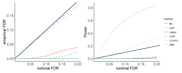
Figure 2: FDR control (left) and power (right) at different nominal levels

5 Data analysis

We illustrate our method by analyzing two GWAS datasets (Morris et al., 2012). A sex-differentiated meta-analysis was performed to test for the association of SNPs with type 2 diabetes. Type 2 diabetes occurs when blood glucose is too high. It affected approximately 329 million individuals in 2015 (Lipton et al., 2016). Identifying replicable SNPs that contribute to disease risk can be instrumental in a full understanding of disease biology and the development of therapeutics. In the first data set, there are $20,219$ type 2 diabetes cases and $54,604$ controls from the male population. In the second data set, there are $14,621$ type 2 diabetes cases and $60,377$ controls from the female population. We aim to find replicable SNPs that are associated with both genders. The datasets are downloaded from DIAbetes Genetics Replication and Meta-analysis Consortium at https://www.diagram-consortium.org/downloads.html. The male group contains summary statistics of $123,535$ SNPs, and the female group contains summary statistics of $118,399$ SNPs. We analyze the paired $p$-values of $m=118,364$ SNPs that are common to both studies, where $y_{1j},j=1,\ldots,m$ denote $p$-values for male population and $y_{2j},j=1,\ldots,m$ denote $p$-values for female population.

The estimated transition matrix is

$$\hat{A}=\begin{pmatrix}0.9840&0.0066&0.0040&0.0055\\ 0.0657&0.9271&0.0004&0.0069\\ 0.0546&0.0010&0.9379&0.0066\\ 0.0501&0.0045&0.0050&0.9403\end{pmatrix},$$

and the stationary probability of different states is

$$\hat{\pi}=(0.779,0.077,0.057,0.087),$$

which is the eigenvector of $\hat{A}$ corresponding to eigenvalue $1.$ The estimated probability density functions of non-null $p$-values, $\hat{f}_{1}$ and $\hat{f}_{2}$, are plotted in Figure 3.

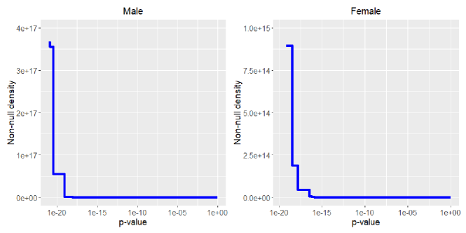
Figure 3: Estimates of $\hat{f}_{1}$ and $\hat{f}_{2}$ in two type 2 diabetes studies

Next, we compare our method to the competing methods. The results of different methods at the FDR level $q=10^{-5}$ are summarized in Figure 4. The MaxP procedure is the most conservative with $176$ findings, and all of them are identified by other methods. Our method has $1,604$ findings, among which $1,202$ are uniquely identified by our method.

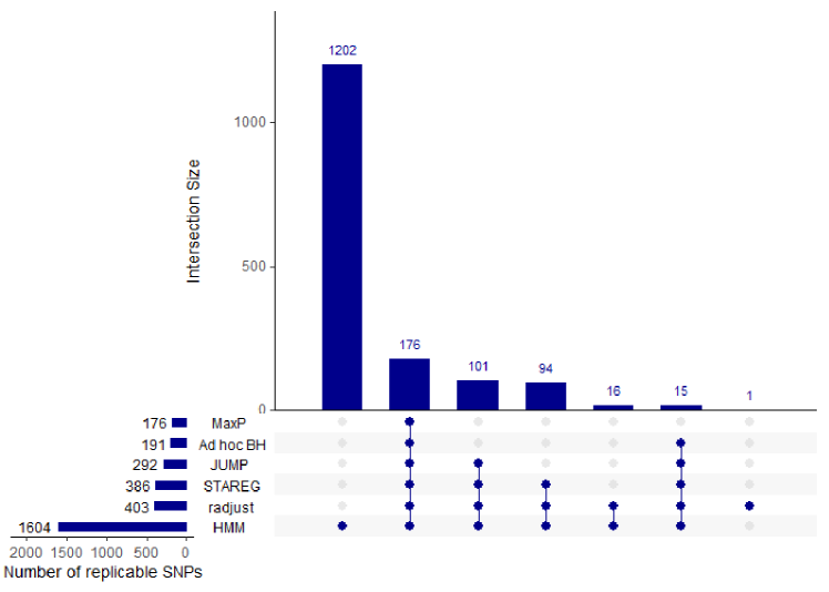
Figure 4: Replicability analysis results of type 2 diabetes data

Among these $1,202$ unique findings, $107$ are recorded in the NHGRI-EBI GWAS Catalog (Sollis et al., 2023), which reports associations with type 2 diabetes in published GWAS at SNP level.

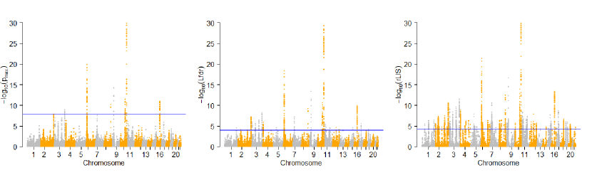
Figure 5: The Manhattan plots of type 2 diabetes GWASs based on $p_{\rm max}$, ${\rm Lfdr}$ and ${\rm rLIS}$. The horizontal blue lines denote the FDR cutoffs of $1\times 10^{-5}$ produced by maxP, STAREG and our method.

Figure 5 presents the Manhattan plots of MaxP, STAREG and our method. In Figure 5, the vertical axes are $-\log_{10}$ transformations of test statistics for replicability analysis. They are $p_{\rm max}$ for MaxP, ${\rm Lfdr}$ for STAREG and ${\rm rLIS}$ for our method. Then we map the remaining SNPs to genes by R package snpGeneSets (Mei et al., 2016). The other $1,095$ SNPs are mapped to $77$ genes, many of which have been reported to be related to type 2 diabetes in previous literature. For example, JAZF1, CDC123, THADA, ADAMTS9-AS2 and NOTCH2 were reported to be associated with type 2 diabetes (Zeggini et al., 2008). JAZF1 is a key transcriptional regulator of ribosome biogenesis, global protein, and insulin translation and has a significant association with type 2 diabetes (Kobiita et al., 2020). 33 SNPs are mapped to JAZF1 such as rs10245867 (rLIS: 2.64e-06; Male $p$-value: 1.03e-08; Female $p$-vale: 6.64e-05). ADAMTS9 can increase the risk of type 2 diabetes through impairment of insulin sensitivity (Graae et al., 2019). 25 SNPs are mapped to ADAMTS9, such as rs11914351 (rLIS: 3.71e-05; Male $p$-value: 8.53e-4; Female $p$-value: 5.70e-2). Increased expression of NOTCH2 may play a role in the pathogenesis of type 2 diabetes, and they may contribute to poor control of the glycemic state (Ghanem et al., 2020). 9 SNPs are mapped to NOTCH2, such as rs10127888 (rLIS: 4.44e-05; Male $p$-value: 2.82e-2; Female $p$-value: 1.52e-2).

6 Concluding remarks

In this paper, we propose a robust and powerful inference of high-dimensional replicability analysis accounting for dependence. We deal with summary statistics such as $p$-values from each study instead of the raw data since summary statistics are easier to access and store. We capture the local dependence of $p$-values by a hidden Markov model. We account for the heterogeneity of different studies by joint hidden states, allowing non-null density functions to have different distributions and estimating them non-parametrically. Furthermore, we obtain the identifiability condition of the unknown parameters and functions, consistency of estimated parameters and functions, and the asymptotic false discovery rate control. Simulation studies demonstrate valid false discovery rate control and higher power of our method. GWAS data analysis provides new biological insights that otherwise cannot be obtained using existing methods.

For the maximum likelihood estimation with a hidden Markov model, theoretical results such as the rate of convergence is desirable, and we leave it as future work. We use two studies to illustrate the main ideas. In theory, our approach can be extended to more than two studies. In practice, for $n$ studies, the total number of possible states is $2^{n}$, which is computationally prohibitive, and a new approach is warranted.

Supplementary Materials

Appendix A Proof of main results

A.1 Proof of Proposition 1

Proof.

Since the spaces of the transition matrix $A$ and stationary probability $\pi$ are bounded and closed with finite dimensions, they are compact. We just need to show the decreasing density function space $\mathcal{H}$ is compact under the Hellinger distance $d_{H}(\cdot,\cdot)$.

Consider any Cauchy sequence $\{g_{n}\}_{n=1}^{\infty}\subseteq\mathcal{H}$. Our goal is to show there exists some $g\in\mathcal{H}$ such that $d_{H}(g_{n},g)\rightarrow 0$ as $n\rightarrow\infty$. Denote $h_{n}=g_{n}^{1/2}$ for all $n=1,2,\ldots$. Then

$$\int_{0}^{1}g_{n}(y){\rm d}y=\int_{0}^{1}h_{n}^{2}(y){\rm d}y=\|h_{n}\|_{2}^{2}=1,$$

which means that $h_{n}\in L^{2}[0,1]$. Since $L^{2}[0,1]$ is compact, there exists some $h\in L^{2}[0,1]$ satisfying

$$\|h_{n}-h\|_{2}^{2}=\int_{0}^{1}\{h_{n}(y)-h(y)\}^{2}{\rm d}y\rightarrow 0\text{ as }n\rightarrow\infty.$$

Denote $g=h^{2}$. Our goal is to show that $g\in\mathcal{H}$: $g$ is a non-increasing density function.

We next show that $\int_{0}^{1}g(y){\rm d}y=1$ by contradiction. Note that $\int_{0}^{1}g(y){\rm d}y=\|h\|_{2}^{2}$. Assume $\|h\|_{2}\neq 1$ and denote $\delta=|\|h\|_{2}-1|>0$. Thus

$$\|h_{n}-h\|_{2}^{2}= \int_{0}^{1}\{h_{n}(y)-h(y)\}^{2}{\rm d}y$$

$$= \|h_{n}\|_{2}^{2}+\|h\|_{2}^{2}-2\int_{0}^{1}h_{n}(y)h(y){\rm d}y$$

$$\geq \|h_{n}\|_{2}^{2}+\|h\|_{2}^{2}-2\|h_{n}\|_{2}\|h\|_{2}$$

$$= (\|h\|_{2}-1)^{2}=\delta^{2}>0,$$

which is contradictory to the fact that $\|h_{n}-h\|_{2}\rightarrow 0$. Then we can conclude that $\|h\|_{2}^{2}=\int_{0}^{1}g(y){\rm d}y=1.$

Next, we show that $h$ is also non-increasing. For any $\varepsilon>0$, denote

$$E_{n}(\varepsilon)=\{y:|h_{n}(y)-h(y)|>\varepsilon\}.$$ (A.1)

Denote $\mu(\cdot)$ as the Lebesgue measure. Thus

$$\varepsilon\mu\{E_{n}(\varepsilon)\}^{1/2}= \left(\int_{E_{n}(\varepsilon)}\varepsilon^{2}dy\right)^{1/2}$$

$$\leq \left(\int_{E_{n}(\varepsilon)}|h_{n}(y)-h(y)|^{2}dy\right)^{1/2}$$

$$\leq \left(\int_{0}^{1}|h_{n}(y)-h(y)|^{2}dy\right)^{1/2}$$

$$= \|h_{n}-h\|_{2}^{2}\to 0\text{ as }n\to\infty,$$

which implies that $h_{n}$ converges to $h$ in measure, or equivalently, for any $\varepsilon>0$,

$$\lim_{n\to\infty}\mu(E_{n}\{\varepsilon)\}=0.$$

By the theorem of Riesz [Riesz, 1928], there exists a subsequence $\{h_{n_{k}}\}$ of $\{h_{n}\}$, such that $h_{n_{k}}\rightarrow h$ almost everywhere. Since $h_{n_{k}}$ are non-increasing, we could conclude that $h$ is also non-increasing.

In conclusion, $g=h^{2}\in\mathcal{H}$ and consequently, $\mathcal{H}$ is compact with respect to the Hellinger distance $d_{H}(\cdot,\cdot)$. ∎

A.2 Proof of Theorem 3.1

For any $\phi\in\Phi$ with $d(\phi,\phi_{0})$, define the conditional distribution of $(y_{1j},y_{2j})_{j=1}^{m}$ given $s_{1}=k,k=0,1,2,3$ as

$$\ell_{m}(k;\phi):= f^{(k)}(y_{11},y_{21};\phi)\sum_{s_{2}}\dots\sum_{s_{m}}a_{k,s_{2}}(\phi)f^{(s_{2})}(y_{12},y_{22};\phi)\prod_{j=3}^{m}a_{s_{j-1},s_{j}}(\phi)f^{(s_{j})}(y_{1j},y_{2j};\phi),$$

where $s_{j}$ denotes the hidden state of the $j$th gene for $j=1,\ldots,m$. Denote the largest $\ell_{m}(k;\phi)$ for $k=0,1,2,3$

$$q_{m}(\phi):=\max_{k=0,1,2,3}\ell_{m}(k;\phi).$$

Then the likelihood function $p_{m}(\phi)=p_{m}\left((y_{1j},y_{2j})_{j=1}^{m};\phi\right)$ satisfies

$$p_{m}(\phi)= \sum_{k=0,1,2,3}\pi_{k}(\phi)\ell_{m}(k;\phi)\leq q_{m}(\phi),$$ (A.2)

where $\pi_{k}(\phi)=P_{\phi}(s_{j}=k)$ for $j=1,\ldots,m$; $k=0,1,2,3$ and satisfies $\sum_{k=0}^{3}\pi_{k}(\phi)=1$.

In addition, assume $q_{m}(\phi)=\ell_{m}(k_{0};\phi)$ for some $k_{0}\in\{0,1,2,3\}$. Then

$$p_{m}(\phi)= \sum_{k=0,1,2,3}\pi_{k}(\phi)\ell_{m}(k;\phi)\geq\pi_{k_{0}}(\phi)\ell_{m}(k_{0};\phi)\geq\varepsilon_{0}q_{m}(\phi),$$ (A.3)

where (A.3) holds due to (C2): $\pi_{k}(\phi)\geq\varepsilon_{0}$ for all $k=0,1,2,3$.

Therefore, combining (A.2) and (A.3) and taking the logarithm, we have

$$\log\left(\varepsilon_{0}\right)\leq\log\frac{p_{m}(\phi)}{q_{m}(\phi)}\leq 0.$$ (A.4)

Dividing (A.4) by $m$, we have

$$\frac{1}{m}\log\left(\varepsilon_{0}\right)\leq\frac{1}{m}\log p_{m}(\phi)-\frac{1}{m}\log q_{m}(\phi)\leq 0.$$ (A.5)

Letting $m\rightarrow\infty$, the lower bound of inequality (A.5) tends to $0$. Hence $m^{-1}\log q_{m}(\phi)$ and $m^{-1}\log p_{m}(\phi)$ converges to the same limit in probability. Taking the expectation on all terms of inequality (A.5), we know $m^{-1}E_{\phi_{0}}\log q_{m}(\phi)$ has the same limit as $m^{-1}E_{\phi_{0}}\log p_{m}(\phi)$. By Theorem 2 in Leroux [1992], there exists some $H(\phi_{0},\phi)<\infty$ satisfying

$$\lim_{m\rightarrow\infty}\frac{1}{m}E_{\phi_{0}}\{\log p_{m}(\phi)\} =H(\phi_{0},\phi),\text{ and }$$

$$\lim_{m\rightarrow\infty}\frac{1}{m}\log p_{m}(\phi) =H(\phi_{0},\phi)\text{ almost surely under }\phi_{0}.$$

We also have

$$\lim_{m\rightarrow\infty}\frac{1}{m}E_{\phi_{0}}\{\log q_{m}(\phi)\} =H(\phi_{0},\phi),\text{ and }$$

$$\lim_{m\rightarrow\infty}\frac{1}{m}\log q_{m}(\phi) =H(\phi_{0},\phi)\text{ almost surely under }\phi_{0}.$$

Replacing $\phi$ by $\phi_{0}$, we get the limit $H(\phi_{0},\phi_{0})$. Lemma 6 in Leroux [1992] gives that $H(\phi_{0},\phi)<H(\phi_{0},\phi_{0})$ for $\phi\neq\phi_{0}$. Letting $\varepsilon=\{H(\phi_{0},\phi_{0})-H(\phi_{0},\phi)\}/2$, there exists $m_{\varepsilon}$ such that,

$$\frac{1}{m_{\varepsilon}}E_{\phi_{0}}\{\log q_{m_{\varepsilon}}(\phi)\}<H(\phi_{0},\phi)+\varepsilon=H(\phi_{0},\phi_{0})-\varepsilon.$$ (A.6)

Denote $O_{\phi,r}=\{\phi^{\prime}\in\Phi:d(\phi^{\prime},\phi)<r\}$ as a ball centered at $\phi$ with radius $r>0$, where $d(\phi^{\prime},\phi)$ is the distance between $\phi^{\prime}$ and $\phi$ defined in (3.1). $E_{\phi_{0}}[\{\log(\sup_{\phi^{\prime}\in O_{\phi,r}}q_{m_{\varepsilon}}(\phi^{\prime}))\}^{+}]<\infty$ by (C4). Therefore, $E_{\phi_{0}}[\{\log(\sup_{\phi^{\prime}\in O_{\phi,r}}q_{m_{\varepsilon}}(\phi^{\prime}))\}^{+}]$ is a bounded monotone increasing function of $r$. Since $f_{1}(\phi),f_{2}(\phi)$ are continuous functions of $\phi$, $p_{m}(\phi)$ and $q_{m}(\phi)$ are also continuous. By the Monotone Convergence Theorem and the continuity of $q_{m_{\varepsilon}}(\phi)$, we have

$$\frac{1}{m_{\varepsilon}}E_{\phi_{0}}\left\{\log\left(\sup_{\phi^{\prime}\in O_{\phi,r}}q_{m_{\varepsilon}}(\phi^{\prime})\right)\right\}\rightarrow\frac{1}{m_{\varepsilon}}E_{\phi_{0}}\left\{\log q_{m_{\varepsilon}}(\phi)\right\}\text{ as }r\rightarrow 0.$$

Then there exists $r_{0}>0$, such that

$$\frac{1}{m_{\varepsilon}}E_{\phi_{0}}\left\{\log\left(\sup_{\phi^{\prime}\in O_{\phi,r_{0}}}q_{m_{\varepsilon}}(\phi^{\prime})\right)\right\}< \frac{1}{m_{\varepsilon}}E_{\phi_{0}}\{\log q_{m_{\varepsilon}}(\phi)\}+\varepsilon/2$$

$$< H(\phi_{0},\phi_{0})-\varepsilon/2,$$ (A.7)

where the second inequality holds due to (A.6).

By the continuity of $p_{m}(\phi)$ and $q_{m}(\phi)$, it follows from (A.5) that

$$\frac{1}{m}\log\left(\varepsilon_{0}\right)\leq\frac{1}{m}\log\left\{\sup_{\phi^{\prime}\in O_{\phi,r}}p_{m}(\phi^{\prime})\right\}-\frac{1}{m}\log\left\{\sup_{\phi^{\prime}\in O_{\phi,r}}q_{m}(\phi^{\prime})\right\}\leq 0.$$

Thus, $m^{-1}\log\{\sup_{\phi^{\prime}\in O_{\phi,r}}p_{m}(\phi^{\prime})\}$ and $m^{-1}\log\{\sup_{\phi^{\prime}\in O_{\phi,r}}q_{m}(\phi^{\prime})\}$ converge to the same limit in probability. Define

$$J(\phi_{0},\phi;O_{\phi,r})=\lim_{m\rightarrow\infty}\frac{1}{m}E_{\phi_{0}}\left\{\log\left(\sup_{\phi^{\prime}\in O_{\phi,r}}q_{m}(\phi^{\prime})\right)\right\}.$$

In addition, we have

$$\frac{1}{m}\log\left\{\sup_{\phi^{\prime}\in O_{\phi,r}}q_{m}(\phi^{\prime})\right\} \rightarrow J(\phi_{0},\phi;O_{\phi,r})\text{ in probability, and }$$

$$\frac{1}{m}\log\left\{\sup_{\phi^{\prime}\in O_{\phi,r}}p_{m}(\phi^{\prime})\right\} \rightarrow J(\phi_{0},\phi;O_{\phi,r})\text{ in probability}.$$ (A.8)

By the construction of $q_{m}(\phi)=q_{m}((y_{1j},y_{2j})_{j=1}^{m};\phi)$, Lemma 3 of Leroux [1992] shows that $\log q_{m}((y_{1j},y_{2j})_{j=1}^{m};\phi)$ is subadditive, which means for any sequence $(y_{1j},y_{2j})_{j=1}^{m}$,

$$\log q_{s+t}((y_{1j},y_{2j})_{j=1}^{s+t};\phi)\leq\log q_{s}((y_{1j},y_{2j})_{j=1}^{s};\phi)+\log q_{t}((y_{1j},y_{2j})_{j=s+1}^{s+t};\phi).$$

By the property of subadditive processes [Fekete, 1923],

$$J(\phi_{0},\phi;O_{\phi,r})=\inf_{m}\frac{1}{m}E_{\phi_{0}}\left\{\log\left(\sup_{\phi^{\prime}\in O_{\phi,r}}q_{m}(\phi^{\prime})\right)\right\}$$

which implies that

$$J(\phi_{0},\phi;O_{\phi,r})\leq\frac{1}{m_{\varepsilon}}E_{\phi_{0}}\left\{\log\left(\sup_{\phi^{\prime}\in O_{\phi,r}}q_{m_{\varepsilon}}(\phi^{\prime})\right)\right\}.$$ (A.9)

Consequently, by (A.8), (A.9) and (A.7), we have as $m\rightarrow\infty$,

$$\frac{1}{m}\log\left\{\sup_{\phi^{\prime}\in O_{\phi,r}}p_{m}(\phi^{\prime})\right\}\rightarrow J(\phi_{0},\phi;O_{\phi,r})\text{ in probability, and }$$

$$J(\phi_{0},\phi;O_{\phi,r})\leq \frac{1}{m_{\varepsilon}}E_{\phi_{0}}\left\{\log\left(\sup_{\phi^{\prime}\in O_{\phi,r}}q_{m_{\varepsilon}}(\phi^{\prime})\right)\right\}$$

$$< H(\phi_{0},\phi_{0})-\varepsilon/2.$$ (A.10)

Next, we use (A.10) to show the consistency of $\hat{\phi}_{m}$. Let $C$ be any closed subset of $\Phi$, not containing $\phi_{0}$. Since $\Phi$ is compact, $C$ is also compact and is covered by the union of finite open sets $\bigcup_{h=1}^{d}O_{\phi_{h},r}$, where $\{\phi_{1},\ldots,\phi_{d}\}$ is a finite set in $C$.

Therefore,

$$\sup_{\phi\in C}\left\{\log p_{m}(\phi)-\log p_{m}(\phi_{0})\right\}$$

$$\leq \max_{1\leq h\leq d}\left[m\left\{\frac{1}{m}\log\left(\sup_{\phi\in O_{\phi_{h},r}}p_{m}(\phi)\right)-\frac{1}{m}\log p_{m}(\phi_{0})\right\}\right]$$

$$\rightarrow -\infty\text{ in probability},$$

where the limit in the last line holds due to (A.10) and that $m^{-1}\log p_{m}(\phi_{0})\to H(\phi_{0},\phi_{0})$ almost surely as $m\to\infty$ by Birkhoff’s ergodic theorem [Birkhoff, 1931]. Since $\hat{\phi}_{m}$ is a maximum likelihood estimator, $\log p_{m}(\hat{\phi}_{m})\geq\log p_{m}(\phi_{0})$. Therefore, $\hat{\phi}_{m}$ cannot be in $C$.

In other words, for any open set $O_{\phi_{0},r}\subseteq\Phi$ containing $\phi_{0}$, $\hat{\phi}_{m}$ must be in $O_{\phi,r}$ for large $m$. Letting $r\rightarrow 0$, we conclude that $\hat{\phi}_{m}\rightarrow\phi_{0}$ in probability.

A.3 FDR control under oracle case

We consider the case that $\phi_{0}=(A,f_{1},f_{2})$ is known. The following theorem shows that FDR can be controlled under the oracle case.

Theorem A.1.

Under the oracle case where $\phi_{0}$ is known, denote ${\rm rLIS}_{j}=P_{\phi_{0}}(s_{j}\in\{0,1,2\}\mid(y_{1j},y_{2j})_{j=1}^{m})$ for $j=1,\ldots,m$. Order the test statistics ${\rm rLIS}_{(1)}\leq\ldots\leq{\rm rLIS}_{(m)}$ with the corresponding null hypotheses $H_{0(1)},\ldots,H_{0(m)}$. For a pre-specified false discovery rate level $q$, we have the following procedure

$$R= \max\left\{r:\frac{1}{r}\sum_{j=1}^{r}{\rm rLIS}_{(j)}\leq q\right\},\text{ and }$$

$$\text{ reject }H_{0(j)}\text{ for }j=1,\ldots,R.$$

Then the testing procedure can control the FDR at level $q$.

Proof.

Denote $R$ as the number of total rejections and $V$ as the number of false rejections. If we reject the replicability null hypothesis $H_{0j}$ if ${\rm rLIS}_{j}\leq\lambda$ for some threshold $\lambda$, then $\lambda$ satisfies

$${\rm rLIS}_{(R)}\leq\lambda<{\rm rLIS}_{(R+1)}.$$

Let $\lambda={\rm rLIS}_{(R)}$ for simplicity.

Therefore,

$${\rm FDR}= E\left\{\frac{V}{R\vee 1}\right\}$$

$$= E\left\{E\left(\frac{V}{R\vee 1}\bigg{|}(y_{1j},y_{2j})_{j=1}^{m}\right)\right\}$$

$$= E\left\{\frac{1}{R\vee 1}E\left(V\mid(y_{1j},y_{2j})_{j=1}^{m}\right)\right\}.$$

The last equality holds because $R$ is a function of $(y_{1j},y_{2j})_{j=1}^{m}$. Since $V=\sum_{j=1}^{m}I({\rm rLIS}_{j}\leq\lambda,s_{j}\in\{0,1,2\})=\sum_{j=1}^{R}I(s_{(j)}\in\{0,1,2\})$, we have

$$E\left(V\mid(y_{1j},y_{2j})_{j=1}^{m}\right)= \sum_{j=1}^{R}P(s_{(j)}\in\{0,1,2\}\mid(y_{1j},y_{2j})_{j=1}^{m})=\sum_{j=1}^{R}{\rm rLIS}_{(j)}.$$

Consequently,

$${\rm FDR}=E\left\{\frac{1}{R\vee 1}\sum_{j=1}^{R}{\rm rLIS}_{(j)}\right\}\leq q.$$

∎

A.4 Proof of Theorem 3.2

First, we introduce some notations used in the proof. Consider an infinite hidden Markov model with hidden states $\{S_{j}\}_{-\infty}^{\infty}$ and $p$-values $(y_{1j},y_{2j})_{-\infty}^{\infty}$. Denote the following test statistics

$$T_{j}= P_{\phi_{0}}(s_{j}\in\{0,1,2\}\mid(y_{1j},y_{2j})_{1}^{m}),$$

$$\hat{T}_{j}= P_{\hat{\phi}_{m}}(s_{j}\in\{0,1,2\}\mid(y_{1j},y_{2j})_{1}^{m}),$$

$$T_{j}^{\infty}= P_{\phi_{0}}(s_{j}\in\{0,1,2\}\mid(y_{1j},y_{2j})_{-\infty}^{\infty}),$$

$$\hat{T}_{j}^{\infty}= P_{\hat{\phi}_{m}}(s_{j}\in\{0,1,2\}\mid(y_{1j},y_{2j})_{-\infty}^{\infty}).$$

For any test statistics $\xi_{j}\in\{T_{j},\hat{T}_{j},T_{j}^{\infty},\hat{T}_{j}^{\infty}\}$ corresponding to the null hypothesis $H_{0j}$, consider the testing procedure based on ordered $\xi_{(1)}\leq\ldots\leq\xi_{(m)}$ with corresponding null hypotheses $H_{0(1)},\ldots,H_{0(m)}$. We have the number of rejections given by

$$R_{0}=\max\left\{r:\frac{1}{r}\sum_{j=1}^{r}\xi_{(j)}\leq q\right\}.$$ (A.11)

We reject $H_{0(j)}$ for $j=1,\ldots,R_{0}$. An equivalent algorithm is

$$\lambda_{0}=\sup\left\{\lambda\in(0,1):\frac{\sum_{j=1}^{m}\xi_{j}I(\xi_{j}\leq\lambda)}{\left\{\sum_{j=1}^{m}I(\xi_{j}\leq\lambda)\right\}\vee 1}\leq q\right\}.$$ (A.12)

The rejection threshold can be written as $\lambda_{0}=\xi_{(R_{0})}$. The total number of false rejections is $V_{0}=\sum_{j=1}^{m}I(\xi_{j}\leq\lambda_{0}\text{ and }s_{j}\in\{0,1,2\})$. Replacing $\xi_{j}$ by $T_{j},\hat{T}_{j},T_{j}^{\infty}$ and $\hat{T}_{j}^{\infty}$, the number of rejections and number of false rejections are denoted by $(R,V)$, $(\hat{R},\hat{V})$, $(R^{\infty},V^{\infty})$ and $(\hat{R}^{\infty},\hat{V}^{\infty})$. Moreover, we define the corresponding rejection thresholds as $\hat{\lambda}_{\mathrm{OR}},\hat{\lambda}_{\mathrm{rLIS}},\hat{\lambda}_{\mathrm{OR}}^{\infty},\hat{\lambda}_{\mathrm{rLIS}}^{\infty}$.

Next, we consider the distribution of $T_{j}^{\infty}$. Since $\{S_{j}\}_{-\infty}^{\infty}$ is stationary, irreducible, and aperiodic, the two-sided generalization of Theorem 6.1.3 in Durrett [2019] implies that $\{T_{j}^{\infty}\}$ is ergodic. Therefore, $T_{j}^{\infty}$ are identically distributed. Denote the cumulative distribution function of $T_{j}^{\infty}$ as

$$P_{\phi_{0}}(T_{j}^{\infty}\leq t)=G^{\infty}(t).$$

Denote the conditional cumulative distribution function of $T_{j}^{\infty}$ given $s_{j}=k$ as

$$P_{\phi_{0}}(T_{j}^{\infty}\leq t\mid s_{j}=k)=G_{k}^{\infty}(t)\text{ for }k=0,1,2,3.$$

Thus

$$G^{\infty}(t)=\pi_{0}G_{0}^{\infty}(t)+\pi_{1}G_{1}^{\infty}(t)+\pi_{2}G_{2}^{\infty}(t)+\pi_{3}G_{3}^{\infty}(t).$$

Let

$$\alpha_{*}=\inf\{0\leq t\leq 1:G^{\infty}(t)=1\}.$$ (A.13)

By the forward-backward algorithm [Baum et al., 1970],

$$T_{j}^{\infty}=\frac{\sum_{s_{j}=0}^{2}\alpha_{j}(s_{j})\beta_{j}(s_{j})}{\sum_{s_{j}=0}^{3}\alpha_{j}(s_{j})\beta_{j}(s_{j})},$$

where $\alpha_{j}(s_{j})=P_{\phi_{0}}((y_{1t},y_{2t})_{t=-\infty}^{j},s_{j})$ and $\beta_{j}(s_{j})=P_{\phi_{0}}((y_{1t},y_{2t})_{t=j+1}^{\infty}\mid s_{j})$. $\alpha_{j}(\cdot)$ and $\beta_{j}(\cdot)$ can be derived recursively by $\alpha_{j+1}(s_{j+1})=\sum_{s_{j}=0}^{3}\alpha_{j}(s_{j})a_{s_{j},s_{j+1}}f^{(s_{j}+1)}(y_{1,j+1},y_{2,j+1})$ and $\beta_{j}(s_{j})=\sum_{s_{j+1}=0}^{3}\beta_{j+1}(s_{j+1})f^{(s_{j+1})}(y_{1,j+1},y_{2,j+1})$. Since the joint distribution of $(y_{1j},y_{2j})_{-\infty}^{\infty}$ is continuous, and $T_{j}^{\infty}$ is a continuous map from $(y_{1j},y_{2j})_{-\infty}^{\infty}$ to (0, 1), the probability density function of $T_{j}^{\infty}$ is positive and continuous. It suffices to show that $G^{\infty}$ is strictly increasing in $(0,\alpha_{*})$. For some threshold $\lambda>0$, define the number of rejections and false rejections as

$$R_{\lambda}^{\infty}= \sum_{j=1}^{m}I(T_{j}^{\infty}\leq\lambda),$$

$$V_{\lambda}^{\infty}= \sum_{j=1}^{m}I(T_{j}^{\infty}\leq\lambda,s_{j}\in\{0,1,2\}).$$

Thus we have the expectations

$$E(R_{\lambda}^{\infty})= mG^{\infty}(\lambda),$$

$$E(V_{\lambda}^{\infty})= m(\pi_{0}G_{0}^{\infty}(\lambda)+\pi_{1}G_{1}^{\infty}(\lambda)+\pi_{2}G_{2}^{\infty}(\lambda)).$$

Therefore, the marginal false discovery rate is

$$Q_{\text{OR}}^{\infty}(\lambda)=E(V_{\lambda}^{\infty})/E(R_{\lambda}^{\infty})=(\pi_{0}G_{0}^{\infty}(\lambda)+\pi_{1}G_{1}^{\infty}(\lambda)+\pi_{2}G_{2}^{\infty}(\lambda))/G^{\infty}(\lambda).$$

Theorem 1 of Sun and Cai [2009] implies that $Q_{\text{OR}}^{\infty}(\lambda)$ is increasing in $\lambda$. Define the threshold based on the marginal false discovery rate as

$$\lambda_{\text{OR}}^{\infty}=\sup\{\lambda:Q_{\text{OR}}^{\infty}(\lambda)\leq q\}.$$

Since $G^{\infty}(t)=1$ is equivalent to the statement that $G_{s}^{\infty}(t)=1$ for $s=0,1,2,3$, we have

$$Q_{\mathrm{OR}}^{\infty}(\alpha_{*})=\pi_{0}+\pi_{1}+\pi_{2}>q$$

under (C2) with $\pi_{3}<1-q$. Without loss of generality, we assume $\lambda_{\mathrm{OR}}^{\infty}<\alpha_{*}.$

With the notations above, we will prove Theorem 3.2 as follows. In Step 1, we show that the total number of rejections $R$ and $\hat{R}$ converge to infinity almost surely. In Step 2, we show that $E|R/\hat{R}-1|\rightarrow 0$ and $E|V/\hat{V}-1|\rightarrow 0$ as $m\to\infty$. Finally, we show the asymptotic false discovery rate control in Step 3.

Step 1. Asymptotic behavior of rejection numbers.

Recall that $\hat{\lambda}_{\mathrm{OR}}^{\infty}$ and $\hat{\lambda}_{\mathrm{rLIS}}^{\infty}$ are the corresponding rejection threshold given by $\{T_{j}^{\infty}\}_{j=1}^{m}$ and $\{\hat{T}_{j}^{\infty}\}_{j=1}^{m}$. First, we show $\hat{\lambda}_{\mathrm{OR}}^{\infty}\rightarrow\lambda_{\mathrm{OR}}^{\infty}$ and $\hat{\lambda}_{\mathrm{rLIS}}^{\infty}\rightarrow\lambda_{\mathrm{OR}}^{\infty}$ in probability by Lemma 1.

Lemma 1.

Assume (C1)-(C4) hold. $\hat{\lambda}_{\mathrm{OR}}^{\infty}\rightarrow\lambda_{\mathrm{OR}}^{\infty}$ and $\hat{\lambda}_{\mathrm{rLIS}}^{\infty}\rightarrow\lambda_{\mathrm{OR}}^{\infty}$ in probability.

We next show $\hat{R}\rightarrow\infty$ almost surely. For simplicity, denote $(y_{1j},y_{2j})_{j=j_{1}}^{j_{2}}$ as $y_{j_{1}}^{j_{2}}$ for any $j_{1}<j_{2}$. By (C2), $\varepsilon_{0}\leq a_{lk}(\phi)\leq 1$ for all $l,k$ and (C5), for any $k,k^{\prime}=0,1,2,3$, $f^{(k^{\prime})}(y_{1,j+1},y_{2,j+1};\phi)/f^{(k)}(y_{1,j+1},y_{2,j+1};\phi)\leq\rho_{0}(y_{1,j+1},y_{2,j+1})$. Then for any states $k,k^{\prime}$ and $l=0,1,2,3$,

$$\frac{P_{\phi}(S_{j+1}=k^{\prime}\mid S_{j}=l,y_{1}^{m})}{P_{\phi}(S_{j+1}=k\mid S_{j}=l,y_{1}^{m})}$$

$$= \frac{P_{\phi}(S_{j+1}=k^{\prime},S_{j}=l,y_{1}^{m})}{P_{\phi}(S_{j+1}=k,S_{j}=l,y_{1}^{m})}$$

$$= \frac{P_{\phi}(S_{j+1}=k^{\prime},y_{1}^{m}\mid S_{j}=l)}{P_{\phi}(S_{j+1}=k,y_{1}^{m}\mid S_{j}=l)}$$

$$= \frac{\sum_{k_{0}=0}^{3}P_{\phi}(S_{j+1}=k^{\prime},S_{j+2}=k_{0},y_{1}^{m}\mid S_{j}=l)}{\sum_{k_{0}=0}^{3}P_{\phi}(S_{j+1}=k,S_{j+2}=k_{0},y_{1}^{m}\mid S_{j}=l)}$$

$$= \frac{P_{\phi}(y_{1}^{j}\mid S_{j}=l;\phi)\sum_{k_{0}=0}^{3}a_{lk^{\prime}}(\phi)a_{k^{\prime}k_{0}}(\phi)f^{(k^{\prime})}(y_{1,j+1},y_{2,j+1};\phi)P_{\phi}(y_{j+2}^{m}\mid S_{j+2}=k_{0};\phi)}{P_{\phi}(y_{1}^{j}\mid S_{j}=l;\phi)\sum_{k_{0}=0}^{3}a_{lk}(\phi)a_{kk_{0}}(\phi)f^{(k)}(y_{1,j+1},y_{2,j+1};\phi)P_{\phi}(y_{j+2}^{m}\mid S_{j+2}=k_{0};\phi)}$$

$$= \frac{f^{(k^{\prime})}(y_{1,j+1},y_{2,j+1};\phi)\sum_{k_{0}=0}^{3}a_{lk^{\prime}}(\phi)a_{k^{\prime}k_{0}}(\phi)P_{\phi}(y_{j+2}^{m}\mid S_{j+2}=k_{0};\phi)}{f^{(k)}(y_{1,j+1},y_{2,j+1};\phi)\sum_{k_{0}=0}^{3}a_{lk}(\phi)a_{kk_{0}}(\phi)P_{\phi}(y_{j+2}^{m}\mid S_{j+2}=k_{0};\phi)}$$

$$\leq \frac{f^{(k^{\prime})}(y_{1,j+1},y_{2,j+1};\phi)\sum_{k_{0}=0}^{3}P_{\phi}(y_{j+2}^{m}\mid S_{j+2}=k_{0};\phi)}{f^{(k)}(y_{1,j+1},y_{2,j+1};\phi)\sum_{k_{0}=0}^{3}\varepsilon_{0}^{2}P_{\phi}(y_{j+2}^{m}\mid S_{j+2}=k_{0};\phi)}$$

$$= \varepsilon_{0}^{-2}\frac{f^{(k^{\prime})}(y_{1,j+1},y_{2,j+1};\phi)}{f^{(k)}(y_{1,j+1},y_{2,j+1};\phi)}$$

$$\leq \varepsilon_{0}^{-2}\rho_{0}(y_{1,j+1},y_{2,j+1}).$$

Let $\tau_{0}(y_{1},y_{2})=(1+3\varepsilon_{0}^{-2}\rho_{0}(y_{1},y_{2}))^{-1}$. Since $\sum_{k^{\prime}=0}^{3}P_{\phi}(S_{j+1}=k^{\prime}\mid S_{j}=l,y_{1}^{m})=1$, we conclude that for all $k,l=0,1,2,3$,

$$P_{\phi}(S_{j+1}=k\mid S_{j}=l,y_{1}^{m})= \frac{P_{\phi}(S_{j+1}=k\mid S_{j}=l,y_{1}^{m})}{\sum_{k^{\prime}=0}^{3}P_{\phi}(S_{j+1}=k^{\prime}\mid S_{j}=l,y_{1}^{m})}$$

$$= \frac{1}{1+\sum_{k^{\prime}\neq k}\frac{P_{\phi}(S_{j+1}=k^{\prime}\mid S_{j}=l,y_{1}^{m})}{P_{\phi}(S_{j+1}=k\mid S_{j}=l,y_{1}^{m})}}$$

$$\geq \{1+3\varepsilon_{0}^{-2}\rho_{0}(y_{1,j+1},y_{2,j+1})\}^{-1}.$$

Define

$$\tau_{0}(y_{1,j+1},y_{2,j+1})=\{1+3\varepsilon_{0}^{-2}\rho_{0}(y_{1,j+1},y_{2,j+1})\}^{-1}.$$

Then

$$P_{\phi}(S_{j+1}=k\mid S_{j}=l,y_{1}^{m})\geq\tau_{0}(y_{1,j+1},y_{2,j+1}).$$ (A.14)

Then we apply Lemma 2 below to show $R\rightarrow\infty$ and $\hat{R}\rightarrow\infty$ almost surely as $m\rightarrow\infty$.

Lemma 2.

If (A.14) and (C1)-(C3) hold, then $R/m\geq G^{\infty}(q/2)>0$ and $\hat{R}/m\geq G^{\infty}(q/2)>0$ almost surely.

Step 2. Convergence of $R/\hat{R}$ and $V/\hat{V}$ in expectation.

In Step 2, we show $E|R/\hat{R}-1|\rightarrow 0$ and $E|V/\hat{V}-1|\rightarrow 0$ under the general case that $0<\lambda_{\rm{OR}}^{\infty}<\alpha_{*}$.

Lemma 3.

If $0<\lambda_{\text{OR}}^{\infty}<\alpha_{*}$, then $E|R/\hat{R}-1|\rightarrow 0$ and $E|V/\hat{V}-1|\rightarrow 0$ as $m\to\infty$.

When $\lambda_{\rm OR}\geq\alpha_{*}$, $R/m$ tends to $1$ as $m\to\infty$, which means all the null hypotheses will be rejected. This is not a feasible case.

Step 3. Asymptotic FDR control.

We have

$$\frac{\hat{V}}{\hat{R}\vee 1}-\frac{V}{R\vee 1}\leq \frac{\hat{V}}{\hat{R}\vee 1}\left(1-\frac{V}{\hat{V}\vee 1}\right)+\frac{V}{R\vee 1}\left(\frac{R\vee 1}{\hat{R}\vee 1}-1\right).$$

Since $\hat{V}/(\hat{R}\vee 1)\leq 1$, we have

$$0\leq\bigg{|}E\left\{\frac{\hat{V}}{\hat{R}\vee 1}\left(1-\frac{V}{\hat{V}\vee 1}\right)\right\}\bigg{|}\leq E\bigg{|}\frac{\hat{V}}{\hat{R}\vee 1}\left(1-\frac{V}{\hat{V}\vee 1}\right)\bigg{|}\leq E\bigg{|}1-\frac{V}{\hat{V}\vee 1}\bigg{|}.$$

By Lemma 3, we have

$$E\left\{\frac{\hat{V}}{\hat{R}\vee 1}\left(1-\frac{V}{\hat{V}\vee 1}\right)\right\}\rightarrow 0\text{ as }m\to\infty.$$

Similarly, we also have

$$E\left\{\frac{V}{R\vee 1}\left(\frac{R}{\hat{R}\vee 1}-1\right)\right\}\rightarrow 0\text{ as }m\to\infty.$$

Therefore,

$${\rm FDR}-{\rm FDR}_{\rm OR}=E\left(\frac{\hat{V}}{\hat{R}\vee 1}\right)-E\left(\frac{V}{R\vee 1}\right)\leq 0\text{ as }m\rightarrow\infty.$$

Since ${\rm FDR}_{\rm OR}\leq q$ by Theorem A.1, we know ${\rm FDR}$ is asymptotically controlled.

Appendix B Proof of lemmas

B.1 Proof of Lemma 1

Proof.

Recall that

$$\hat{\lambda}_{\mathrm{OR}}^{\infty}= \sup\left\{t:\hat{Q}_{\mathrm{OR}}^{\infty}(t)\leq q\right\},$$

$$\lambda_{\mathrm{OR}}^{\infty}= \sup\left\{t:Q_{\mathrm{OR}}^{\infty}(t)\leq q\right\},$$

where

$$\hat{Q}_{\mathrm{OR}}^{\infty}(t)= \frac{\sum_{j=1}^{m}I(T_{j}^{\infty}\leq t)T_{j}^{\infty}}{\sum_{j=1}^{m}I(T_{j}^{\infty}\leq t)},$$ (B.1)

$$Q_{\mathrm{OR}}^{\infty}(t)= \frac{\pi_{0}G_{0}^{\infty}(t)+\pi_{1}G_{1}^{\infty}(t)+\pi_{2}G_{2}^{\infty}(t)}{G^{\infty}(t)}.$$

Since $T_{1}^{\infty}=P(s_{1}\in\{0,1,2\}\mid(y_{1j},y_{2j})_{-\infty}^{\infty})$, it is a funtion of $(y_{1j},y_{2j})_{-\infty}^{\infty}$. Thus

$$E\left\{I(T_{1}^{\infty}\leq t)T_{1}^{\infty}\right\}= E\left\{I(T_{1}^{\infty}\leq t)E\left[I(s_{1}\in\{0,1,2\})\mid(y_{1j},y_{2j})_{-\infty}^{\infty}\right]\right\}$$

$$= E\left\{E[I(T_{1}^{\infty}\leq t,s_{1}\in\{0,1,2\})\mid(y_{1j},y_{2j})_{-\infty}^{\infty}]\right\}$$

$$= P\left(T_{1}^{\infty}\leq t,s_{1}\in\{0,1,2\}\right)$$

$$= \pi_{0}G_{0}^{\infty}(t)+\pi_{1}G_{1}^{\infty}(t)+\pi_{2}G_{2}^{\infty}(t),\text{ and }$$

$$E\left\{I(T_{1}^{\infty}\leq t)\right\}= G^{\infty}(t).$$

Brikhoff’s ergodic theorem [Birkhoff, 1931] gives

$$\frac{1}{m}\sum_{j=1}^{m}I(T_{j}^{\infty}\leq t)T_{j}^{\infty}\rightarrow \pi_{0}G_{0}^{\infty}(t)+\pi_{1}G_{1}^{\infty}(t)+\pi_{2}G_{2}^{\infty}(t)\text{ almost surely for any }t,$$

$$\frac{1}{m}\sum_{j=1}^{m}I(T_{j}^{\infty}\leq t)\rightarrow G^{\infty}(t)\text{ almost surely for any }t.$$

Consequently,

$$\hat{Q}_{\mathrm{OR}}^{\infty}(t)\rightarrow Q_{\mathrm{OR}}^{\infty}(t)\text{ almost surely for any }t\text{ such that }G^{\infty}(t)>0.$$ (B.2)

In addition, $G^{\infty}(\lambda^{\infty}_{\rm OR})>0$. Therefore,

$$P\bigg{(}\lim_{m\rightarrow\infty}\hat{Q}_{\mathrm{OR}}^{\infty}(\lambda_{\mathrm{OR}}^{\infty})\leq q\bigg{)}= P\bigg{(}\lim_{m\rightarrow\infty}\big{(}\hat{Q}_{\mathrm{OR}}^{\infty}(\lambda_{\mathrm{OR}}^{\infty})-Q_{\mathrm{OR}}^{\infty}(\lambda_{\mathrm{OR}}^{\infty})\big{)}+Q_{\mathrm{OR}}^{\infty}(\lambda_{\mathrm{OR}}^{\infty})\leq q\bigg{)}=1,$$

which implies that $P(\lim_{m\rightarrow\infty}\hat{\lambda}_{\mathrm{OR}}^{\infty}\geq\lambda_{\mathrm{OR}}^{\infty})=1$, or equivalently,

$$\hat{\lambda}_{\mathrm{OR}}^{\infty}\geq\lambda_{\mathrm{OR}}^{\infty}\text{ almost surely.}$$ (B.3)

By construction, $\hat{Q}_{\mathrm{OR}}^{\infty}(t)$ is an increasing step function with jump at $T_{(j)}^{\infty}$. For $T_{(j)}^{\infty}\leq t<T_{(j+1)}^{\infty}$, construct the lower bound of $\hat{Q}_{\rm OR}^{\infty}(t)$ as

$$\hat{L}_{\mathrm{OR}}^{\infty}(t)= \frac{T_{(j+1)}^{\infty}-t}{T_{(j+1)}^{\infty}-T_{(j)}^{\infty}}\hat{Q}_{\mathrm{OR}}^{\infty}(T_{(j-1)}^{\infty})+\frac{t-T_{(j)}^{\infty}}{T_{(j+1)}^{\infty}-T_{(j)}^{\infty}}\hat{Q}_{\mathrm{OR}}^{\infty}(T_{(j)}^{\infty}).$$

Then $\hat{L}_{\mathrm{OR}}^{\infty}(t)$ is strictly increasing in $t$. We also have

$$0\leq\hat{Q}_{\mathrm{OR}}^{\infty}(t)-\hat{L}_{\mathrm{OR}}^{\infty}(t)\leq \hat{Q}_{\mathrm{OR}}^{\infty}(T_{(j)}^{\infty})-\hat{Q}_{\mathrm{OR}}^{\infty}(T_{(j-1)}^{\infty})$$

$$= \frac{(j-1)T_{(j)}^{\infty}-\sum_{k=1}^{j-1}T_{(k)}^{\infty}}{j(j-1)}$$

$$\leq \frac{1}{j}$$

$$= \frac{1}{R^{\infty}(t)},$$

where $R^{\infty}(t)=\sum_{k=1}^{m}1(T_{k}^{\infty}\leq t)$ denotes the number of rejections yielded by threshold $t$, satisfying $R^{\infty}(t)=j$ if $T_{(j)}^{\infty}\leq t<T_{(j+1)}^{\infty}$. By Birkhoff’s ergodic theorem [Birkhoff, 1931], $R^{\infty}(t)/m\to G^{\infty}(t)$ almost surely as $m\to\infty$. Then for any $t\in[0,1]$,

$$\hat{Q}_{\mathrm{OR}}^{\infty}(t)-\hat{L}_{\mathrm{OR}}^{\infty}(t)\rightarrow 0\text{ almost surely}.$$

By (B.2), $\hat{L}_{\mathrm{OR}}^{\infty}(t)\rightarrow Q_{\mathrm{OR}}^{\infty}(t)$ almost surely for any $t\in[0,1]$.

Denote

$$\hat{\lambda}_{\mathrm{L,OR}}^{\infty}=\sup\{t\in(0,1):\hat{L}_{\mathrm{OR}}^{\infty}(t)\leq q\}.$$

As $\hat{Q}_{\mathrm{OR}}^{\infty}(t)\geq\hat{L}_{\mathrm{OR}}^{\infty}(t)$ with probability $1$, we have

$$\hat{\lambda}_{\mathrm{OR}}^{\infty}\leq\hat{\lambda}_{\mathrm{L,OR}}^{\infty}\text{ with probability }1.$$ (B.4)

By (B.3), we also have $\hat{\lambda}_{\rm L,OR}^{\infty}\geq\lambda_{\rm OR}^{\infty}$ almost surely.

We claim that $\hat{\lambda}_{\mathrm{L,OR}}^{\infty}\rightarrow\lambda_{\mathrm{OR}}^{\infty}$ in probability. If not, there exist $\varepsilon_{2}>0$ and $\eta_{0}>0$ such that for any $M>0$, there exists $m_{1}\geq M$ satisfying

$$P(K_{m_{1}}^{1})\geq 2\eta_{0},$$

where $K_{m_{1}}^{1}$ denotes the even that $\hat{\lambda}_{\mathrm{L,OR}}^{\infty}-\lambda_{\mathrm{OR}}^{\infty}>\varepsilon_{2}$.

Let

$$2\delta_{1}=Q_{\mathrm{OR}}^{\infty}(\lambda_{\mathrm{OR}}^{\infty}+\varepsilon_{2})-q>0.$$

Since $\hat{L}_{\mathrm{OR}}^{\infty}(t)\rightarrow Q_{\mathrm{OR}}^{\infty}(t)$ in probability for any $t\in[0,1]$, there exists $M>0$, such that for any $m_{2}\geq M$,

$$P(K_{m_{2}}^{2})\geq 1-\eta_{0},$$

where $K_{m_{2}}^{2}$ denotes the event that $|\hat{L}_{\mathrm{OR}}^{\infty}(\lambda_{\mathrm{OR}}^{\infty}+\varepsilon_{2})-Q_{\mathrm{OR}}^{\infty}(\lambda_{\mathrm{OR}}^{\infty}+\varepsilon_{2})|<\delta_{1}$.

Without loss of generality, assume $m_{1}=m_{2}=m$. Letting $K_{m}=K_{m}^{1}\bigcap K_{m}^{2}$, we have

$$P(K_{m})= 1-P((K_{m}^{1})^{c}\cup(K_{m}^{2})^{c})$$

$$\geq 1-\{(1-2\eta_{0})+\eta_{0}\}$$

$$= \eta_{0}.$$

Thus $K_{m}$ has positive probability.

Additionally, $\hat{L}_{\mathrm{OR}}^{\infty}(t)$ is strictly increasing over $t$ with probability $1$. On $K_{m}$, we have

$$q= \hat{L}_{\mathrm{OR}}^{\infty}(\hat{\lambda}_{\mathrm{L,OR}}^{\infty})$$

$$> \hat{L}_{\mathrm{OR}}^{\infty}(\lambda_{\mathrm{OR}}^{\infty}+\varepsilon_{2})$$

$$> Q_{\mathrm{OR}}^{\infty}(\lambda_{\mathrm{OR}}^{\infty}+\varepsilon_{2})-\delta_{1}$$

$$= q+\delta_{1},$$

which is a contradiction. Thus we must have $\hat{\lambda}_{\mathrm{L,OR}}^{\infty}\rightarrow\lambda_{\mathrm{OR}}^{\infty}$ in probability. Furthermore, by (B.3) and (B.4),

$$\hat{\lambda}_{\mathrm{OR}}^{\infty}\rightarrow\lambda_{\mathrm{OR}}^{\infty}\text{ in probability as }m\rightarrow\infty.$$

$\hat{\lambda}_{\rm rLIS}^{\infty}\to\lambda_{\rm OR}^{\infty}$ in probability can be shown in the same way. ∎

B.2 Proof of Lemma 2

Proof.

Define $M_{d}^{+}(j,\phi)=\max_{k,l=0,1,2,3}P_{\phi}(S_{j}=k\mid y_{1}^{m},S_{j-d}=l)$. Similarly, define $M_{d}^{-}(j,\phi)=\min_{k,l=0,1,2,3}P_{\phi}(S_{j}=k\mid y_{1}^{m},S_{j-d}=l)$. We need to show that

$$|M_{d}^{+}(j,\phi)-M_{d}^{-}(j,\phi)|\leq\prod_{i=j-d+1}^{j-1}\{1-2\tau_{0}(y_{1i},y_{2i})\}.$$ (B.5)

Since $\varepsilon_{0}\leq 1/4$ and $\rho_{0}(y_{1i},y_{2i})\geq 1$ with probability $1$, we have $\tau_{0}(y_{1i},y_{2i})=\{1+\varepsilon_{0}^{2}\rho_{0}(y_{1i},y_{2i})\}^{-1}\leq 1/13$ with probability $1$. Thus $1-2\tau_{0}(y_{1i},y_{2i})>0$ with probability $1$ for any $i=1,\ldots,m.$ We have

$$P_{\phi}(S_{j}=k\mid y_{1}^{m},S_{j-d}=l)= \sum_{k^{\prime}=0}^{3}P_{\phi}(S_{j}=k,S_{j-d+1}=k^{\prime}\mid y_{1}^{m},S_{j-d}=l)$$

$$= \sum_{k^{\prime}=0}^{3}P_{\phi}(S_{j}=k\mid y_{1}^{m},S_{j-d+1}=k^{\prime})P_{\phi}(S_{j-d+1}=k^{\prime}\mid y_{1}^{m},S_{j-d}=l).$$

Since $P_{\phi}(S_{j-d+1}=k^{\prime}\mid y_{1}^{m},S_{j-d}=l)\geq\tau_{0}(y_{1,j-d+1},y_{2,j-d+1})$, we have

$$M_{d}^{+}(j,\phi)\leq \{1-\tau_{0}(y_{1,j-d+1},y_{2,j-d+1})\}M_{d-1}^{+}(j,\phi)+\tau_{0}(y_{1,j-d+1},y_{2,j-d+1})M_{d-1}^{-}(j,\phi),$$

and similarly,

$$M_{d}^{-}(j,\phi)\geq \{1-\tau_{0}(y_{1,j-d+1},y_{2,j-d+1})\}M_{d-1}^{-}(j,\phi)+\tau_{0}(y_{1,j-d+1},y_{2,j-d+1})M_{d-1}^{+}(j,\phi).$$

Therefore,

$$M_{d}^{+}(j,\phi)-M_{d}^{-}(j,\phi)\leq \{1-2\tau_{0}(y_{1,j-d+1},y_{2,j-d+1})\}\{M_{d-1}^{+}(j,\phi)-M_{d-1}^{-}(j,\phi)\}$$

$$\leq \prod_{i=j-d+1}^{j-1}\{1-2\tau_{0}(y_{1i},y_{2i})\}\{M_{1}^{+}(j,\phi)-M_{1}^{-}(j,\phi)\}.$$

Since $M_{1}^{+}(j,\phi)-M_{1}^{-}(j,\phi)\leq 1$, we know (B.5) is true. We have the similar definitions $N_{d}^{+}(j,\phi)=\max_{k,l=0,1,2,3}P_{\phi}(S_{j}=k\mid y_{1}^{m},S_{j+d}=l)$ and $N_{d}^{-}(j,\phi)=\min_{k,l=0,1,2,3}P_{\phi}(S_{j}=k\mid y_{1}^{m},S_{j+d}=l)$. We also have

$$|N_{d}^{+}(j,\phi)-N_{d}^{-}(j,\phi)|\leq\prod_{i=j+1}^{j+d-1}\{1-2\tau_{0}(y_{1i},y_{2i})\}.$$ (B.6)

We move to the second step. Let $L<m/2$. For any $j$, let $L_{1}=1\vee(j-L)$ and $L_{2}=m\wedge(j+L)$. We claim that when $L_{1}>1$ and $L_{2}<m$,

$$|P_{\phi}(S_{j}\in\{0,1,2\}\mid y_{1}^{m})-P_{\phi}(S_{j}\in\{0,1,2\}\mid y_{-\infty}^{\infty})|$$

$$< 3\prod_{i=L_{1}+1}^{j-1}\exp\{-2\tau_{0}(y_{1i},y_{2i})\}+3\prod_{i=j+1}^{L_{2}-1}\exp\{-2\tau_{0}(y_{1i},y_{2i})\}.$$ (B.7)

We have

$$|P_{\phi}(S_{j}\in\{0,1,2\}\mid y_{1}^{m})-P_{\phi}(S_{j}\in\{0,1,2\}\mid y_{-\infty}^{\infty})|$$

$$\leq |P_{\phi}(S_{j}\in\{0,1,2\}\mid y_{1}^{m})-P_{\phi}(S_{j}\in\{0,1,2\}\mid y_{-\infty}^{m})|$$

$$+|P_{\phi}(S_{j}\in\{0,1,2\}\mid y_{-\infty}^{m})-P_{\phi}(S_{j}\in\{0,1,2\}\mid y_{-\infty}^{\infty})|.$$

We just need to show

$$|P_{\phi}(S_{j}\in\{0,1,2\}\mid y_{1}^{m})-P_{\phi}(S_{j}\in\{0,1,2\}\mid y_{-\infty}^{m})|\leq 3\prod_{i=L_{1}+1}^{j-1}\exp\{-2\tau_{0}(y_{1i},y_{2i})\}$$

and

$$|P_{\phi}(S_{j}\in\{0,1,2\}\mid y_{-\infty}^{m})-P_{\phi}(S_{j}\in\{0,1,2\}\mid y_{-\infty}^{\infty})|\leq 3\prod_{i=j+1}^{L_{2}-1}\exp\{-2\tau_{0}(y_{1i},y_{2i})\}.$$

We have for $k=0,1,2$,

$$|P_{\phi}(S_{j}=k\mid y_{1}^{m})-P_{\phi}(S_{j}=k\mid y_{-\infty}^{m})|$$

$$= \bigg{|}\sum_{l=0}^{3}P_{\phi}(S_{j}=k\mid S_{j-L}=l,y_{1}^{m})P_{\phi}(S_{j-L}=l\mid y_{1}^{m})$$

$$-\sum_{l^{\prime}=0}^{3}P_{\phi}(S_{j}=k\mid S_{j-L}=l^{\prime},y_{1}^{m})P_{\phi}(S_{j-L}=l^{\prime}\mid y_{-\infty}^{m})\bigg{|}$$

$$\leq \max_{l,l^{\prime}=0,1,2,3}|P_{\phi}(S_{j}=k\mid S_{j-L}=l,y_{1}^{m})-P_{\phi}(S_{j}=k\mid S_{j-L}=l^{\prime},y_{1}^{m})|$$

$$\leq M_{L}^{+}(j,\phi)-M_{L}^{-}(j,\phi)$$

$$\leq \prod_{i=L_{1}+1}^{j-1}\{1-2\tau_{0}(y_{1i},y_{2i})\}$$

$$\leq \prod_{i=L_{1}+1}^{j-1}\exp\{-2\tau_{0}(y_{1i},y_{2i})\}.$$

Then

$$|P_{\phi}(S_{j}\in\{0,1,2\}\mid y_{1}^{m})-P_{\phi}(S_{j}\in\{0,1,2\}\mid y_{-\infty}^{m})|$$

$$\leq \sum_{k=0}^{2}|P_{\phi}(S_{j}=k\mid y_{1}^{m})-P_{\phi}(S_{j}=k\mid y_{-\infty}^{m})|$$

$$\leq 3\prod_{i=L_{1}+1}^{j-1}\exp\{-2\tau_{0}(y_{1i},y_{2i})\}.$$

Similarly, we also have

$$|P_{\phi}(S_{j}\in\{0,1,2\}\mid y_{-\infty}^{m})-P_{\phi}(S_{j}\in\{0,1,2\}\mid y_{-\infty}^{\infty})|\leq 3\prod_{i=j+1}^{L_{2}-1}\exp\{-2\tau_{0}(y_{1i},y_{2i})\}.$$

Therefore, (B.2) is true. Then we consider the expectations.

$$E_{\phi_{0}}|P_{\phi}(S_{j}\in\{0,1,2\}\mid y_{1}^{m})-P_{\phi}(S_{j}\in\{0,1,2\}\mid y_{-\infty}^{\infty})|$$

$$\leq E_{\phi_{0}}\left[3\prod_{i=L_{1}+1}^{j-1}\exp\{-2\tau_{0}(y_{1i},y_{2i})\}+3\prod_{i=j+1}^{L_{2}-1}\exp\{-2\tau_{0}(y_{1i},y_{2i})\}\right]$$

$$= E_{\phi_{0}}\left\{E_{\phi_{0}}\left[3\prod_{i=L_{1}+1}^{j-1}\exp\{-2\tau_{0}(y_{1i},y_{2i})\}+3\prod_{i=j+1}^{L_{2}-1}\exp\{-2\tau_{0}(y_{1i},y_{2i})\}\bigg{|}S_{1},\ldots,S_{m}\right]\right\}$$

$$= E_{\phi_{0}}\left\{3\prod_{i=L_{1}+1}^{j-1}E_{\phi_{0}}\left[\exp\{-2\tau_{0}(y_{1i},y_{2i})\}\mid S_{i}\right]+3\prod_{i=j+1}^{L_{2}-1}E_{\phi_{0}}\left[\exp\{-2\tau_{0}(y_{1i},y_{2i})\}\mid S_{i}\right]\right\}.$$

By (C5) and the construction of $\tau_{0}(Y_{1j},Y_{2j})$, we have $P_{\phi_{0}}(\tau_{0}(Y_{1j},Y_{2j})>0\mid S_{j}=k)=1$ for all $k=0,1,2,3$. Let

$$\beta_{0}=\max_{k=0,1,2,3}E_{\phi_{0}}\left[\exp\{-2\tau_{0}(y_{11},y_{21})\}\mid S_{1}=k\right],$$ (B.8)

then we have $\beta_{0}<1$. Therefore, for some $C_{0}>0$,

$$E_{\phi_{0}}|P_{\phi}(S_{j}\in\{0,1,2\}\mid y_{1}^{m})-P_{\phi}(S_{j}\in\{0,1,2\}\mid y_{-\infty}^{\infty})|\leq C_{0}\beta_{0}^{L}.$$ (B.9)

By Lévy’s upward theorem [Williams, 1991], $P_{\phi}(S_{0}\in\{0,1,2\}\mid(y_{1j},y_{2j})_{-N}^{N})\rightarrow T_{0}^{\infty}$ almost surely as $N\rightarrow\infty$. Next, we show that $G^{\infty}(q/2)=P_{\phi}(T_{0}^{\infty}\leq q/2)>0$. Note that

$$P_{\phi}(T_{0}^{\infty}\leq q/2)$$

$$= P_{\phi}\left(\frac{P_{\phi}(S_{j}\in\{0,1,2\}\mid(y_{1j},y_{2j})_{-\infty}^{\infty})}{P_{\phi}(S_{j}=3\mid(y_{1j},y_{2j})_{-\infty}^{\infty})}\leq\frac{q/2}{1-q/2}\right)$$

$$= P_{\phi}\left(\frac{\sum_{k=0}^{2}\pi_{k}P_{\phi}((y_{1j},y_{2j})_{-\infty}^{\infty}\mid S_{j}=k)}{\pi_{3}P_{\phi}((y_{1j},y_{2j})_{-\infty}^{\infty}\mid S_{j}=3)}\leq\frac{q/2}{1-q/2}\right)$$

$$= P_{\phi}\bigg{(}\sum_{k=0}^{2}\frac{\sum_{l_{1},l_{2}=0,1,2,3}P_{\phi}((y_{1j},y_{2j})_{-\infty}^{-1}\mid S_{-1}=l_{1})a_{l_{1}k}a_{kl_{2}}P_{\phi}((y_{1j},y_{2j})_{1}^{\infty}\mid S_{1}=l_{2})}{\sum_{l_{1},l_{2}=0,1,2,3}P_{\phi}((y_{1j},y_{2j})_{-\infty}^{-1}\mid S_{-1}=l_{1})a_{l_{1}3}a_{3l_{2}}P_{\phi}((y_{1j},y_{2j})_{1}^{\infty}\mid S_{1}=l_{2})}$$

$$\quad\cdot\frac{\pi_{k}f^{(k)}(y_{10},y_{20})}{\pi_{3}f^{(3)}(y_{10},y_{20})}\leq\frac{q/2}{1-q/2}\bigg{)}.$$

By (C2), $\varepsilon_{0}\leq a_{kl}\leq 1$ for all $k,l=0,1,2,3$. Then we have

$$\varepsilon_{0}^{2}\leq\frac{\sum_{l_{1},l_{2}=0,1,2,3}P_{\phi}((y_{1j},y_{2j})_{-\infty}^{-1}\mid S_{-1}=l_{1})a_{l_{1}k}a_{kl_{2}}P_{\phi}((y_{1j},y_{2j})_{1}^{\infty}\mid S_{1}=l_{2})}{\sum_{l_{1},l_{2}=0,1,2,3}P_{\phi}((y_{1j},y_{2j})_{-\infty}^{-1}\mid S_{-1}=l_{1})a_{l_{1}3}a_{3l_{2}}P_{\phi}((y_{1j},y_{2j})_{1}^{\infty}\mid S_{1}=l_{2})}\leq\varepsilon_{0}^{-2}.$$

Consequently,

$$P_{\phi}(T_{0}^{\infty}\leq q/2)\geq P_{\phi}\left\{\varepsilon_{0}^{-2}\left(\frac{\pi_{0}}{\pi_{3}}\frac{1}{f_{1}(y_{10})f_{2}(y_{20})}+\frac{\pi_{1}}{\pi_{3}}\frac{1}{f_{2}(y_{20})}+\frac{\pi_{2}}{\pi_{3}}\frac{1}{f_{1}(y_{10})}\right)\leq\frac{q/2}{1-q/2}\right\}$$

$$= P_{\phi}\left\{\varepsilon_{0}^{2}\frac{q/2}{1-q/2}f_{1}(y_{10})f_{2}(y_{20})-\frac{\pi_{1}}{\pi_{3}}f_{1}(y_{10})-\frac{\pi_{2}}{\pi_{3}}f_{2}(y_{20})-\frac{\pi_{0}}{\pi_{3}}\geq 0\right\}.$$

By (C2), $\lim_{y\rightarrow 0}f_{1}(y)>c$ and $\lim_{y\rightarrow 0}f_{2}(y)>c$. Moreover, two roots of the quadratic equation

$$g_{2}(x)=\varepsilon_{0}^{2}\frac{q/2}{1-q/2}x^{2}-\frac{\pi_{1}+\pi_{2}}{\pi_{3}}x-\frac{\pi_{0}}{\pi_{3}}=0$$

are

$$x_{0}^{(1)}= \frac{\pi_{1}+\pi_{2}-\sqrt{(\pi_{1}+\pi_{2})^{2}+4\varepsilon_{0}^{2}\pi_{0}\pi_{3}q/(2-q)}}{2\varepsilon_{0}^{2}\pi_{3}q/(2-q)}<0\text{ and }$$

$$x_{0}^{(2)}= \frac{\pi_{1}+\pi_{2}+\sqrt{(\pi_{1}+\pi_{2})^{2}+4\varepsilon_{0}^{2}\pi_{0}\pi_{3}q/(2-q)}}{2\varepsilon_{0}^{2}\pi_{3}q/(2-q)}>0.$$

By (C2), for each $k=0,1,2,3$, $\varepsilon_{0}\leq\pi_{k}\leq 1-3\varepsilon_{0}$. Thus

$$x_{0}^{(2)}\leq\frac{1-2\varepsilon_{0}+\sqrt{(1-2\varepsilon_{0})^{2}+4\varepsilon_{0}^{3}(1-3\varepsilon_{0})q/(2-q)}}{2\varepsilon_{0}^{3}q/(2-q)}=c,$$

where $c$ is defined in (C2). Thus $g_{2}(c)>0$ and

$$\varepsilon_{0}^{2}\frac{q/2}{1-q/2}c-\frac{\pi_{1}}{\pi_{3}}> \frac{1}{c}\left(\frac{\pi_{2}}{\pi_{3}}c+\frac{\pi_{0}}{\pi_{3}}\right)>0,\text{ and }$$

$$\varepsilon_{0}^{2}\frac{q/2}{1-q/2}c-\frac{\pi_{2}}{\pi_{3}}> \frac{1}{c}\left(\frac{\pi_{1}}{\pi_{3}}c+\frac{\pi_{0}}{\pi_{3}}\right)>0.$$

By (C2), $\lim_{x_{1}\to 0}f_{1}(x_{1})>c$ and $\lim_{x_{2}\to 0}f_{2}(x_{2})>c$. Since $f_{1},f_{2}$ are continuous, there exist $u_{1},u_{2}\in(0,1)$ such that $f_{1}(x_{1})>c$ and $f_{2}(x_{2})>c$ whenever $0<x_{1}<u_{1}$ and $0<x_{2}<u_{2}$. Consequently, for $0<x_{1}<u_{1}$ and $0<x_{2}<u_{2}$

$$\varepsilon_{0}^{2}\frac{q/2}{1-q/2}f_{2}(x_{2})-\frac{\pi_{1}}{\pi_{3}}>\varepsilon_{0}^{2}\frac{q/2}{1-q/2}c-\frac{\pi_{1}}{\pi_{3}}>0.$$

Therefore,

$$\varepsilon_{0}^{2}\frac{q/2}{1-q/2}f_{1}(x_{1})f_{2}(x_{2})-\frac{\pi_{1}}{\pi_{3}}f_{1}(x_{1})-\frac{\pi_{2}}{\pi_{3}}f_{2}(x_{2})-\frac{\pi_{0}}{\pi_{3}}$$

$$= \left\{\varepsilon_{0}^{2}\frac{q/2}{1-q/2}f_{2}(x_{2})-\frac{\pi_{1}}{\pi_{3}}\right\}f_{1}(x_{1})-\frac{\pi_{2}}{\pi_{3}}f_{2}(x_{2})-\frac{\pi_{0}}{\pi_{3}}$$

$$\geq \left\{\varepsilon_{0}^{2}\frac{q/2}{1-q/2}f_{2}(x_{2})-\frac{\pi_{1}}{\pi_{3}}\right\}c-\frac{\pi_{2}}{\pi_{3}}f_{2}(x_{2})-\frac{\pi_{0}}{\pi_{3}}$$

$$= \left\{\varepsilon_{0}^{2}\frac{q/2}{1-q/2}c-\frac{\pi_{2}}{\pi_{3}}\right\}f_{2}(x_{2})-\frac{\pi_{1}}{\pi_{3}}c-\frac{\pi_{0}}{\pi_{3}}$$

$$\geq \varepsilon_{0}^{2}\frac{q/2}{1-q/2}c^{2}-\frac{\pi_{1}+\pi_{2}}{\pi_{3}}c-\frac{\pi_{0}}{\pi_{3}}=g_{2}(c)>0.$$

Therefore, we have

$$P_{\phi}(T_{0}^{\infty}\leq q/2)\geq P_{\phi}\left\{Y_{10}\in(0,u_{1}),Y_{20}\in(0,u_{2})\right\}>0.$$

and thus we can conclude that $P_{\phi}(T_{0}^{\infty}\leq q/2)>0$.

Finally, we show that $R/m\geq G^{\infty}(q/2)$ and $\hat{R}/m\geq G^{\infty}(q/2)$ almost surely as $m\to\infty$. We consider the case that not all hypotheses are rejected. Recall (A.12). The threshold $\hat{\lambda}_{\rm OR}$ satisfies $\hat{\lambda}_{\rm OR}\geq q$ with probability $1$. It suffices to show that $m^{-1}\sum_{j=1}^{m}I(T_{j}\leq q)\geq G^{\infty}(q/2)$ almost surely as $m\to\infty$. Take $L_{m}=m^{\kappa}$, with $\kappa\in(0,1)$. $L_{m}$ satisfies $L_{m}<m/2$ when $m$ is large enough. For any $j$ satisfying $L_{m}+1<j<m-L_{m}-1$, by (B.2), we have

$$|T_{j}-T_{j}^{\infty}|= |P_{\phi_{0}}(s_{j}\in\{0,1,2\}\mid y_{1}^{m})-P_{\phi_{0}}(s_{j}\in\{0,1,2\}\mid y_{-\infty}^{\infty})|$$

$$< 3\prod_{i=j-L_{m}+1}^{j-1}\exp\{-2\tau_{0}(y_{1i},y_{2i})\}+3\prod_{i=j+1}^{j+L_{m}-1}\exp\{-2\tau_{0}(y_{1i},y_{2i})\}$$

with probability $1$.

Define $d_{j}((y_{1i},y_{2i})_{1}^{m})=3\prod_{i=j-L_{m}+1}^{j-1}\exp\{-2\tau_{0}(y_{1i},y_{2i})\}+3\prod_{i=j+1}^{j+L_{m}-1}\exp\{-2\tau_{0}(y_{1i},y_{2i})\}$. Then $d_{j}((y_{1i},y_{2i})_{1}^{m})$ is ergodic. Thus Brikhoff’s ergodic theorem [Birkhoff, 1931] gives that

$$\frac{1}{m-2L_{m}-1}\sum_{j=L_{m}+1}^{m-L_{m}-1}I(d_{j}>q/2)\rightarrow P_{\phi_{0}}(d_{1}>q/2)\text{ in probability}.$$

Moreover, $E_{\phi_{0}}[d_{j}]<C_{0}\beta_{0}^{L_{m}}$ by the construction of $\beta_{0}$ in (B.8). Then Markov’s inequality gives

$$P_{\phi_{0}}(d_{1}>q/2)\leq\frac{E_{\phi_{0}}[d_{j}]}{q/2}\rightarrow 0\text{ as }L_{m}=m^{\kappa}\rightarrow\infty.$$

Thus

$$\frac{1}{m}\sum_{j=1}^{m}I\left(|T_{j}-T_{j}^{\infty}|>q/2\right)\leq\frac{2L_{m}+1}{m}+\frac{1}{m}\sum_{j=L_{m}+1}^{m-L_{m}-1}I(d_{j}>q/2)\rightarrow 0\text{ in probability}$$

as $m\to\infty$. We use the property that $I(T_{j}\leq q)+I(|T_{j}-T_{j}^{\infty}|>q/2)\geq I(T_{j}^{\infty}\leq q/2)$. Then

$$\frac{1}{m}\sum_{j=1}^{m}I(T_{j}\leq q)+\frac{1}{m}\sum_{j=1}^{m}I(|T_{j}-T_{j}^{\infty}|>q/2)\geq\frac{1}{m}\sum_{j=1}^{m}I(T_{j}^{\infty}\leq q/2).$$

By Birkhoff’s ergodic theorem, we have

$$\frac{1}{m}\sum_{j=1}^{m}I(T_{j}^{\infty}\leq q/2)\rightarrow G^{\infty}(q/2)\text{ almost surely as }m\to\infty.$$

Then we have $m^{-1}\sum_{j=1}^{m}I(T_{j}\leq q)\geq G^{\infty}(q/2)$ almost surely. We have shown that $G^{\infty}(t)>0$ for any $t\in(0,1)$. Therefore, $m^{-1}\sum_{j=1}^{m}I(T_{j}\leq q)\geq G^{\infty}(q/2)>0$ almost surely, which means $R/m\geq G^{\infty}(q/2)$ almost surely. We can use a similar argument to show that $\hat{R}/m\geq G^{\infty}(q/2)$ almost surely. The details are omitted. ∎

B.3 Proof of Lemma 3

Proof.

Note that $R\rightarrow\infty$ almost surely as $m\to\infty$ as shown in Lemma 2. The rejection criteria in (2.9) implies that

$$\frac{1}{R}\sum_{j=1}^{R}T_{(j)}\leq q<\frac{1}{R+1}\sum_{j=1}^{R+1}T_{(j)}.$$

Note that as $m\rightarrow\infty$,

$$E\left|\frac{1}{R}\sum_{j=1}^{R}T_{(j)}-\frac{1}{R+1}\sum_{j=1}^{R+1}T_{(j)}\right|=E\left|\frac{\sum_{j=1}^{R}\left(T_{(j)}-T_{(R+1)}\right)}{R(R+1)}\right|\leq E\left|\frac{1}{R+1}\right|\rightarrow 0.$$

Since

$$0\leq \left|\frac{1}{R}\sum_{j=1}^{R}T_{(j)}-q\right|\leq\left|\frac{1}{R}\sum_{j=1}^{R}T_{(j)}-\frac{1}{R+1}\sum_{j=1}^{R+1}T_{(j)}\right|,$$

we have

$$E\left|\frac{1}{R}\sum_{j=1}^{R}T_{(j)}-q\right|\rightarrow 0\text{ as }m\rightarrow\infty.$$ (B.10)

We can use the same approach to show

$$E\left|\frac{1}{\hat{R}}\sum_{j=1}^{\hat{R}}\hat{T}_{(j)}-q\right|\rightarrow 0\text{ as }m\rightarrow\infty.$$ (B.11)

Therefore, combining (B.10) and (B.11), we have

$$E\left|\frac{1}{\hat{R}}\sum_{j=1}^{\hat{R}}\hat{T}_{(j)}-\frac{1}{R}\sum_{j=1}^{R}T_{(j)}\right|\to 0\text{ as }m\rightarrow\infty.$$ (B.12)

We finish the proof by contradiction. Assume that $\lim_{m\rightarrow\infty}E|R/\hat{R}-1|=0$ does not hold, where $R$ is the total number of rejections by (2.9) when the total number of hypotheses is $m$ and $\hat{R}$ is the total number of rejections by (3.3) when the total number of hypotheses is $m$. Then there is $\varepsilon_{1}>0$ such that, for any $M>0$, there exists some $m\geq M$ satisfying $E|R/\hat{R}-1|>\varepsilon_{1}$. Since

$$E|R/\hat{R}-1|= E\{(1-R/\hat{R})I(\hat{R}>R)\}+E\{(R/\hat{R}-1)I(R>\hat{R})\},$$

$E|R/\hat{R}-1|>\varepsilon_{1}$ implies that either (i) $E\{(1-R/\hat{R})I(\hat{R}>R)\}>\varepsilon_{1}/2$, or (ii) $E\{(R/\hat{R}-1)I(R>\hat{R})\}>\varepsilon_{1}/2$.

We first consider the case that (i) is true. Then $E\{(1-R/\hat{R})I(\hat{R}>R)\}>\varepsilon_{1}/2$ and therefore the event $E_{1}=\{\hat{R}>R\}$ has positive probability. On the event $E_{1}$, we have

$$\left|\frac{1}{\hat{R}}\sum_{j=1}^{\hat{R}}\hat{T}_{(j)}-\frac{1}{R}\sum_{j=1}^{R}T_{(j)}\right|$$

$$= \left|\frac{1}{\hat{R}}\sum_{j=1}^{\hat{R}}\hat{T}_{(j)}-\frac{1}{\hat{R}}\sum_{j=1}^{\hat{R}}T_{(j)}+\frac{1}{\hat{R}}\sum_{j=1}^{\hat{R}}T_{(j)}-\frac{1}{R}\sum_{j=1}^{R}T_{(j)}\right|$$

$$= \left|\frac{1}{\hat{R}}\sum_{j=1}^{\hat{R}}\left(\hat{T}_{(j)}-T_{(j)}\right)+\frac{1}{\hat{R}}\left(\sum_{j=1}^{R}+\sum_{j=R+1}^{\hat{R}}\right)T_{(j)}-\frac{1}{R}\sum_{j=1}^{R}T_{(j)}\right|$$

$$= \left|\frac{1}{\hat{R}}\sum_{j=1}^{\hat{R}}\left(\hat{T}_{(j)}-T_{(j)}\right)+\frac{1}{\hat{R}}\sum_{j=R+1}^{\hat{R}}T_{(j)}-\left(1-\frac{R}{\hat{R}}\right)\frac{1}{R}\sum_{j=1}^{R}T_{(j)}\right|$$

$$\geq \left|\frac{1}{\hat{R}}\sum_{j=R+1}^{\hat{R}}T_{(j)}-\left(1-\frac{R}{\hat{R}}\right)\frac{1}{R}\sum_{j=1}^{R}T_{(j)}\right|-\left|\frac{1}{\hat{R}}\sum_{j=1}^{\hat{R}}\left(\hat{T}_{(j)}-T_{(j)}\right)\right|$$ (B.13)

$$\geq \left|1-\frac{R}{\hat{R}}\right|\left|T_{\left(R+1\right)}-\frac{1}{R}\sum_{j=1}^{R}T_{(j)}\right|-\left|\frac{1}{\hat{R}}\sum_{j=1}^{\hat{R}}\hat{T}_{(j)}-\frac{1}{\hat{R}}\sum_{j=1}^{\hat{R}}T_{(j)}\right|,$$ (B.14)

where (B.13) holds due to triangle inequality $|a+b|\geq|b|-|a|$ and (B.14) holds because

$$\frac{1}{\hat{R}}\sum_{j=R+1}^{\hat{R}}T_{(j)}-\left(1-\frac{R}{\hat{R}}\right)\frac{1}{R}\sum_{j=1}^{R}T_{(j)}$$

$$\geq \frac{1}{\hat{R}}\sum_{j=R+1}^{\hat{R}}T_{(R+1)}-\left(1-\frac{R}{\hat{R}}\right)\frac{1}{R}\sum_{j=1}^{R}T_{(j)}$$

$$= \frac{\hat{R}-R}{\hat{R}}T_{(R+1)}-\left(1-\frac{R}{\hat{R}}\right)\frac{1}{R}\sum_{j=1}^{R}T_{(j)}$$

$$= \left(1-\frac{R}{\hat{R}}\right)\left(T_{(R+1)}-\frac{1}{R}\sum_{j=1}^{R}T_{(j)}\right)\geq 0.$$

We next show that $|T_{(R+1)}-R^{-1}\sum_{j=1}^{R}T_{(j)}|$ in (B.14) is positive with probability $1$. Since the event $\{R^{-1}\sum_{j=1}^{R}T_{(j)}\leq q\}$ has probability $1$, it suffices to show that

$$T_{(R+1)}\geq \lambda_{\mathrm{OR}}^{\infty}\text{ with probability approaching $1$.}$$ (B.15)

$$\lambda_{\rm OR}^{\infty}> q.$$ (B.16)

Since $\hat{\lambda}_{\mathrm{OR}}>q$ with probability $1$, for $0<\gamma<1$ and $\hat{Q}_{\rm OR}$ defined in (B.1), we have

$$\hat{Q}_{\mathrm{OR}}(\hat{\lambda}_{\mathrm{OR}})= \frac{1}{R}\sum_{j=1}^{m}T_{j}I(T_{j}\leq\hat{\lambda}_{\rm OR})$$

$$= \frac{1}{R}\sum_{j=1}^{m}T_{j}I(T_{j}\leq\gamma q)+\frac{1}{R}\sum_{j=1}^{m}T_{j}I(\gamma q<T_{j}\leq\hat{\lambda}_{\mathrm{OR}})$$

$$\leq \gamma q\frac{\sum_{j=1}^{m}I(T_{j}\leq\gamma q)}{\sum_{j=1}^{m}I(T_{j}\leq\hat{\lambda}_{\mathrm{OR}})}+\hat{\lambda}_{\mathrm{OR}}\frac{\sum_{j=1}^{m}I(\gamma q<T_{j}\leq\hat{\lambda}_{\mathrm{OR}})}{\sum_{j=1}^{m}I(T_{j}\leq\hat{\lambda}_{\mathrm{OR}})}.$$ (B.17)

Lemma 1 shows that $\hat{\lambda}_{\mathrm{OR}}^{\infty}\rightarrow\lambda_{\mathrm{OR}}^{\infty}$ in probability, and the construction of $T_{j}$ and $T_{j}^{\infty}$ gives that $\hat{\lambda}_{\rm OR}-\hat{\lambda}_{\rm OR}^{\infty}\rightarrow 0$ in probability. Therefore,

$$\hat{\lambda}_{\rm OR}\to\lambda_{\rm OR}^{\infty}\text{ in probability as }m\to\infty.$$ (B.18)

Similarly, we also have

$$\hat{\lambda}_{\rm rLIS}\to\lambda_{\rm OR}^{\infty}\text{ in probability as }m\to\infty.$$ (B.19)

Combining (B.18) and (B.19), we have

$$\hat{\lambda}_{\rm OR}-\hat{\lambda}_{\rm rLIS}\to 0\text{ in probability as }m\to\infty.$$ (B.20)

By the rejection criteria (2.8) and (2.9), $T_{(R+1)}>\hat{\lambda}_{\rm OR}$ with probability $1$. Thus (B.15) holds. Moreover, for any $\epsilon>0$, $P(|\hat{\lambda}_{\rm OR}-\lambda_{\rm OR}^{\infty}|>\epsilon)\rightarrow 0$ as $m\rightarrow\infty$. Then on the event $|\hat{\lambda}_{\rm OR}-\lambda_{\rm OR}^{\infty}|\leq\epsilon$,

$$\frac{1}{m}\sum_{j=1}^{m}I(T_{j}\leq\hat{\lambda}_{\rm OR})\leq \frac{1}{m}\sum_{j=1}^{m}I(T_{j}\leq\lambda_{\rm OR}^{\infty}+\epsilon),$$

$$\frac{1}{m}\sum_{j=1}^{m}I(T_{j}\leq\hat{\lambda}_{\rm OR})\geq \frac{1}{m}\sum_{j=1}^{m}I(T_{j}\leq\lambda_{\rm OR}^{\infty}-\epsilon).$$

Birkhoff’s ergodic theorem [Birkhoff, 1931] gives that as $m\rightarrow\infty$,

$$\frac{1}{m}\sum_{j=1}^{m}I(T_{j}\leq\lambda_{\rm OR}^{\infty}+\epsilon)\rightarrow G^{\infty}(\lambda_{\rm OR}^{\infty}+\epsilon)\text{ almost surely, and }$$

$$\frac{1}{m}\sum_{j=1}^{m}I(T_{j}\leq\lambda_{\rm OR}^{\infty}-\epsilon)\rightarrow G^{\infty}(\lambda_{\rm OR}^{\infty}-\epsilon)\text{ almost surely.}$$

When $\epsilon$ tends to $0$, the continuity of $G^{\infty}$ gives that as $m\rightarrow\infty$,

$$\frac{1}{m}\sum_{j=1}^{m}I(T_{j}\leq\hat{\lambda}_{\rm OR})\rightarrow G^{\infty}(\lambda_{\rm OR}^{\infty})\text{ almost surely.}$$ (B.21)

Similarly,

$$\frac{1}{m}\sum_{j=1}^{m}I(\hat{T}_{j}\leq\hat{\lambda}_{\rm rLIS})\rightarrow G^{\infty}(\lambda_{\rm OR}^{\infty})\text{ almost surely.}$$ (B.22)

Moreover, by Birkhoff’s ergodic theorem [Birkhoff, 1931], we have

$$\frac{1}{m}\sum_{j=1}^{m}I(T_{j}\leq\gamma q)\rightarrow G^{\infty}(\gamma q)\text{ almost surely.}$$ (B.23)

Combining (B.17), (B.21) and (B.23), we have

$$\hat{Q}_{\mathrm{OR}}(\hat{\lambda}_{\mathrm{OR}})\leq \gamma q\frac{G^{\infty}(\gamma q)}{G^{\infty}(\lambda_{\mathrm{OR}}^{\infty})}+\lambda_{\mathrm{OR}}^{\infty}\frac{G^{\infty}(\lambda_{\mathrm{OR}}^{\infty})-G^{\infty}(\gamma q)}{G^{\infty}(\lambda_{\mathrm{OR}}^{\infty})},$$

with probability approaching $1$. Recall that $\hat{Q}_{\mathrm{OR}}(\hat{\lambda}_{\mathrm{OR}})=R^{-1}\sum_{j=1}^{R}T_{(j)}=q+o_{p}(1)$. Thus for any $\gamma\in(0,1)$,

$$q\leq \gamma q\frac{G^{\infty}(\gamma q)}{G^{\infty}(\lambda_{\mathrm{OR}}^{\infty})}+\lambda_{\mathrm{OR}}^{\infty}\frac{G^{\infty}(\lambda_{\mathrm{OR}}^{\infty})-G^{\infty}(\gamma q)}{G^{\infty}(\lambda_{\mathrm{OR}}^{\infty})}+o(1).$$

Equivlently, we have

$$\lambda_{\mathrm{OR}}^{\infty}\geq \sup_{\gamma\in(0,1)}\left\{q+\frac{q(1-\gamma)G^{\infty}(\gamma q)}{G^{\infty}(\lambda_{\mathrm{OR}}^{\infty})-G^{\infty}(\gamma q)}\right\}>q.$$

Since $G^{\infty}$ is strictly increasing in $(0,\alpha_{*})$ and $\alpha_{*}>\lambda_{\rm OR}^{\infty}$, we have $G^{\infty}(\gamma q)>0$ and $G^{\infty}(\lambda_{\mathrm{OR}}^{\infty})-G^{\infty}(\gamma q)>0$. Therefore, (B.16) holds.

By (B.10), (B.15) and (B.16), we have

$$E\left(T_{(R+1)}-\frac{1}{R}\sum_{j=1}^{R}T_{(R)}\right)$$

$$= E\left(T_{(R+1)}-\lambda_{\rm OR}^{\infty}\right)+(\lambda_{\rm OR}^{\infty}-q)+E\left(q-\frac{1}{R}\sum_{j=1}^{R}T_{(R)}\right)$$

$$\geq \lambda_{\rm OR}^{\infty}-q\text{ as }m\to\infty.$$

It implies that

$$T_{(R+1)}-\frac{1}{R}\sum_{j=1}^{R}T_{(R)}\geq\lambda_{\rm OR}-q\text{ with probability approaching }1.$$ (B.24)

Next, we show

$$E\left|\frac{1}{\hat{R}}\sum_{j=1}^{\hat{R}}\hat{T}_{(j)}-\frac{1}{\hat{R}}\sum_{j=1}^{\hat{R}}T_{(j)}\right|\to 0\text{ as }m\to\infty.$$ (B.25)

Note that

$$\left|\frac{1}{\hat{R}}\sum_{j=1}^{\hat{R}}T_{(j)}-\frac{1}{\hat{R}}\sum_{j=1}^{\hat{R}}\hat{T}_{(j)}\right|\leq \left|\frac{1}{\hat{R}}\sum_{j=1}^{\hat{R}}T_{(j)}-\frac{1}{\hat{R}}\sum_{j=1}^{\hat{R}}T_{(j)}^{\infty}\right|$$

$$+ \left|\frac{1}{\hat{R}}\sum_{j=1}^{\hat{R}}T_{(j)}^{\infty}-\frac{1}{\hat{R}}\sum_{j=1}^{\hat{R}}\hat{T}_{(j)}^{\infty}\right|$$

$$+ \left|\frac{1}{\hat{R}}\sum_{j=1}^{\hat{R}}\hat{T}_{(j)}^{\infty}-\frac{1}{\hat{R}}\sum_{j=1}^{\hat{R}}\hat{T}_{(j)}\right|.$$ (B.26)

Denote $S_{\hat{R}}=\{j:T_{j}\leq T_{(\hat{R})}\}$ and $S_{\hat{R}}^{\infty}=\{j:T_{j}^{\infty}\leq T_{(\hat{R})}^{\infty}\}$. Since $\sum_{j\in S_{\hat{R}}}T_{j}\leq\sum_{j\in S_{\hat{R}}^{\infty}}T_{j}$ and $\sum_{j\in S_{\hat{R}}^{\infty}}T_{j}^{\infty}\leq\sum_{j\in S_{\hat{R}}}T_{j}^{\infty}$, we have

$$\sum_{j\in S_{\hat{R}}}T_{j}-\sum_{j\in S_{\hat{R}}}T_{j}^{\infty}\leq\sum_{j\in S_{\hat{R}}}T_{j}-\sum_{j\in S_{\hat{R}}^{\infty}}T_{j}^{\infty}\leq\sum_{j\in S_{\hat{R}}^{\infty}}T_{j}-\sum_{j\in S_{\hat{R}}^{\infty}}T_{j}^{\infty}.$$

Therefore,

$$\left|\sum_{j\in S_{\hat{R}}}T_{j}-\sum_{j\in S_{\hat{R}}^{\infty}}T_{j}^{\infty}\right|\leq\left|\sum_{j\in S_{\hat{R}}}T_{j}-\sum_{j\in S_{\hat{R}}}T_{j}^{\infty}\right|+\left|\sum_{j\in S_{\hat{R}}^{\infty}}T_{j}-\sum_{j\in S_{\hat{R}}^{\infty}}T_{j}^{\infty}\right|.$$ (B.27)

For $L_{m}=m^{\kappa}$ with $\kappa\in(0,1)$, denote

$$\tilde{S}_{\hat{R}}= \{j\in S_{\hat{R}}:L_{m}+1<j<m-L_{m}-1\}\text{, and}$$

$$\tilde{S}_{\hat{R}}^{\infty}= \{j\in S_{\hat{R}}^{\infty}:L_{m}+1<j<m-L_{m}-1\}.$$

By (B.9), $E|T_{j}-T_{j}^{\infty}|\leq C_{0}\beta_{0}^{L_{m}}$ for $\beta_{0}\in(0,1)$ if $L_{m}+1<j<m-L_{m}-1$. Whenever $j\leq L_{m}+1$ or $j\geq m-L_{m}-1$, $|T_{j}-T_{j}^{\infty}|\leq 1$. Note that Lemma 2 shows that $\hat{R}/m\geq G^{\infty}(q/2)$ almost surely as $m\to\infty$. Therefore, by (B.27),

$$E\left|\frac{1}{\hat{R}}\sum_{j\in S_{\hat{R}}}T_{j}-\frac{1}{\hat{R}}\sum_{j\in S_{\hat{R}}^{\infty}}T_{j}^{\infty}\right|\leq 2E\left(\frac{2L_{m}+1}{\hat{R}}\right)+E\left|\frac{1}{\hat{R}}\sum_{j\in\tilde{S}_{\hat{R}}}(T_{j}-T_{j}^{\infty})\right|+E\left|\frac{1}{\hat{R}}\sum_{j\in\tilde{S}_{\hat{R}}^{\infty}}(T_{j}-T_{j}^{\infty})\right|$$

$$\leq \frac{2(2m^{\kappa}+1)}{mG^{\infty}(q/2)}+2\max_{L_{m}+1<j<m-L_{m}-1}E|T_{j}-T_{j}^{\infty}|$$

$$\leq \frac{2(2m^{\kappa}+1)}{mG^{\infty}(q/2)}+2C_{0}\beta_{0}^{m^{\kappa}}\to 0\text{ as }m\to\infty.$$ (B.28)

Similarly, for $\hat{S}_{\hat{R}}=\{j:\hat{T}_{j}\leq\hat{T}_{(\hat{R})}\}$ and $\hat{S}_{\hat{R}}^{\infty}=\{j:\hat{T}_{j}^{\infty}\leq\hat{T}_{(\hat{R})}^{\infty}\}$, we have

$$E\left|\frac{1}{\hat{R}}\sum_{j\in\hat{S}_{\hat{R}}^{\infty}}\hat{T}_{j}^{\infty}-\frac{1}{\hat{R}}\sum_{j\in\hat{S}_{\hat{R}}}\hat{T}_{j}\right|\leq\frac{2(2m^{\kappa}+1)}{mG^{\infty}(q/2)}+2C_{0}\beta_{0}^{m^{\kappa}}\to 0\text{ as }m\to\infty.$$ (B.29)

Furthermore, denote $S_{\hat{R}}^{\infty}=\{j:T_{j}^{\infty}\leq T_{(\hat{R})}^{\infty}\}$ and $\hat{S}_{\hat{R}}^{\infty}=\{j:\hat{T}_{j}^{\infty}\leq\hat{T}_{(\hat{R})}^{\infty}\}$. By (B.22), we have $\hat{R}/m\to G^{\infty}(\lambda_{\rm OR}^{\infty})$ almost surely as $m\to\infty$. By Birkhoff’s ergodic theorem [Birkhoff, 1931], we have $T_{(\hat{R})}^{\infty}\to\lambda_{\rm OR}^{\infty}$ almost surely as $m\to\infty$. Note that

$$\frac{1}{\hat{R}}\sum_{j\in S_{\hat{R}}^{\infty}}T_{j}^{\infty}= \frac{1}{\hat{R}}\sum_{j\in S_{\hat{R}}^{\infty}}T_{j}^{\infty}I(T_{j}^{\infty}\leq T_{(\hat{R})}^{\infty}).$$

Birkhoff’s ergodic theorem [Birkhoff, 1931] gives that

$$E\left\{\frac{1}{\hat{R}}\sum_{j\in S_{\hat{R}}^{\infty}}T_{j}^{\infty}I(T_{j}^{\infty}\leq T_{(\hat{R})}^{\infty})\right\}\to E\{T_{1}^{\infty}\mid T_{1}^{\infty}\leq\lambda_{\rm OR}^{\infty}\}=\frac{1}{G^{\infty}(\lambda_{\rm OR}^{\infty})}\int_{0}^{\lambda_{\rm OR}^{\infty}}x{\rm d}G^{\infty}(x)\text{ as }m\to\infty.$$

Similarly, we have $\hat{T}_{(\hat{R})}^{\infty}\to\lambda_{\rm OR}^{\infty}$ almost surely as $m\to\infty$ by Birkhoff’s ergodit theorem [Birkhoff, 1931]. Therefore,

$$E\left\{\frac{1}{\hat{R}}\sum_{j\in\hat{S}_{\hat{R}}^{\infty}}\hat{T}_{j}^{\infty}\right\}\to\frac{1}{G^{\infty}(\lambda_{\rm OR}^{\infty})}\int_{0}^{\lambda_{\rm OR}^{\infty}}x{\rm d}G^{\infty}(x)\text{ as }m\to\infty.$$

Therefore, we have

$$E\left|\frac{1}{\hat{R}}\sum_{j\in S_{\hat{R}}^{\infty}}T_{j}^{\infty}-\frac{1}{\hat{R}}\sum_{j\in\hat{S}_{\hat{R}}^{\infty}}\hat{T}_{j}^{\infty}\right|\to 0\text{ as }m\to\infty.$$ (B.30)

Combining (B.26), (B.28), (B.29) and (B.30), we have (B.25).

Then by (B.14), (B.24) and (B.25), for any $M>0$, there exists some $m\geq M$ satisfying

$$E\left|\frac{1}{\hat{R}}\sum_{j=1}^{\hat{R}}\hat{T}_{(j)}-\frac{1}{R}\sum_{j=1}^{R}T_{(j)}\right|$$

$$\geq E\left\{\left|1-\frac{R}{\hat{R}}\right|\cdot I(\hat{R}>R)\cdot\bigg{|}T_{(R+1)}-\frac{1}{R}\sum_{j=1}^{R}T_{(j)}\bigg{|}\right\}-E\bigg{|}\frac{1}{\hat{R}}\sum_{j=1}^{\hat{R}}\hat{T}_{(j)}-\frac{1}{\hat{R}}\sum_{j=1}^{\hat{R}}T_{(j)}\bigg{|}$$

$$> \frac{\varepsilon_{1}}{2}\left|\lambda_{\mathrm{OR}}^{\infty}-q\right|+o(1).$$

This is contradictionary to (B.12). Therefore, (i) does not hold.

Now consider the case when (ii) is true. In this case, $E\{(R/\hat{R}-1)I(R>\hat{R})\}>\varepsilon_{1}/2$ and therefore the event $E_{2}=\{R/\hat{R}>1+\varepsilon_{1}/2\}$ has positive probability. By (B.11) and (B.25), we have

$$(1/\hat{R})\sum_{j=1}^{\hat{R}}T_{(j)}=q\text{ with probability approaching $1$}.$$ (B.31)

Thus $T_{(\hat{R}+1)}\geq q$ with probability $1$. Then we can use a similar method as (B.14) and obtain that on the event $E_{2}$,

$$\left|\frac{1}{R}\sum_{j=1}^{R}T_{(j)}-\frac{1}{\hat{R}}\sum_{j=1}^{\hat{R}}\hat{T}_{(j)}\right|= \left|\frac{1}{\hat{R}}\sum_{j=1}^{\hat{R}}\left(\hat{T}_{(j)}-T_{(j)}\right)+\left(1-\frac{\hat{R}}{R}\right)\left(\frac{1}{\hat{R}}\sum_{j=1}^{\hat{R}}T_{(j)}-\frac{1}{R-\hat{R}}\sum_{j=\hat{R}+1}^{R}T_{(j)}\right)\right|$$

$$\geq \left|1-\frac{\hat{R}}{R}\right|\left|\frac{1}{R-\hat{R}}\sum_{j=\hat{R}+1}^{R}T_{(j)}-\frac{1}{\hat{R}}\sum_{j=1}^{\hat{R}}T_{(j)}\right|-\left|\frac{1}{\hat{R}}\sum_{j=1}^{\hat{R}}\hat{T}_{(j)}-\frac{1}{\hat{R}}\sum_{j=1}^{\hat{R}}T_{(j)}\right|.$$

Let $\eta\in\left(q,\lambda_{\mathrm{OR}}^{\infty}\right),\mathcal{S}_{1}=\left\{j:T_{(\hat{R}+1)}\leq T_{(j)}\leq\eta\right\}$ and $\mathcal{S}_{2}=\left\{j:\eta<T_{(j)}\leq T_{(R)}\right\}$. We know $|\mathcal{S}_{1}|+|\mathcal{S}_{2}|=R-\hat{R}$, where $|\cdot|$ denotes the cardinality of a set. Since $T_{(\hat{R}+1)}\geq q$ with probability $1$, we have

$$\frac{1}{R-\hat{R}}\sum_{j=\hat{R}+1}^{R}T_{(j)}= \frac{1}{R-\hat{R}}\left(\sum_{j\in S_{1}}T_{(j)}+\sum_{j\in S_{2}}T_{(j)}\right)$$

$$\geq \frac{1}{R-\hat{R}}\bigg{(}|\mathcal{S}_{1}|q+|\mathcal{S}_{2}|(\eta-q+q)+o_{p}(1)\bigg{)}$$

$$= q+\frac{\left|\mathcal{S}_{2}\right|}{R-\hat{R}}(\eta-q)+o_{p}(1).$$

We apply the ergodic theorem [Birkhoff, 1931] and continuity of $G^{\infty}$ to obtain

$$\frac{1}{m}\left|\mathcal{S}_{2}\right|= \frac{1}{m}\sum_{j=1}^{m}I\left(\eta<T_{j}\leq T_{(R)}\right)\rightarrow G^{\infty}\left(\lambda_{\mathrm{OR}}^{\infty}\right)-G^{\infty}(\eta)\text{ almost surely}$$

as $m\to\infty.$ Since $T_{(R)}\leq\lambda_{\rm OR}^{\infty}$ with probability $1$ and $T_{(\hat{R}+1)}\geq q$ with probability, we have

$$\frac{1}{m}\left(R-\hat{R}\right)=\frac{1}{m}\sum_{j=1}^{m}I\left(T_{(\hat{R}+1)}\leq T_{j}\leq T_{(R)}\right)\leq G^{\infty}\left(\lambda_{\mathrm{OR}}^{\infty}\right)-G^{\infty}(q)\text{ almost surely}$$

as $m\to\infty.$ Since $|\mathcal{S}_{2}|/(R-\hat{R})\leq 1$, the continuous mapping theorem gives that

$$\frac{1}{R-\hat{R}}\sum_{j=\hat{R}+1}^{R}T_{(j)}\geq q+\frac{G^{\infty}\left(\lambda_{\mathrm{OR}}^{\infty}\right)-G^{\infty}(\eta)}{G^{\infty}\left(\lambda_{\mathrm{OR}}^{\infty}\right)-G^{\infty}(q)}(\eta-q)\text{ almost surely}$$ (B.32)

as $m\to\infty.$ Denote $\nu_{0}=\left[\left\{G^{\infty}\left(\lambda_{\mathrm{OR}}^{\infty}\right)-G^{\infty}(\eta)\right\}/\left\{G\left(\lambda_{\mathrm{OR}}^{\infty}\right)-G(q)\right\}\right](\eta-q)$. Note that $G^{\infty}(t)$, the culmulative distribution function of $T_{j}^{\infty}$, is strictly increasing in $t$ over the interval $\left(0,\alpha_{*}\right)$. It implies that $\nu_{0}>0$. Hence by (B.31) and (B.32), we have

$$\left|\frac{1}{R}\sum_{j=1}^{R}T_{(j)}-\frac{1}{\hat{R}}\sum_{j=1}^{\hat{R}}\hat{T}_{(j)}\right|\geq\left|1-\frac{\hat{R}}{R}\right|\nu_{0}-\bigg{|}\frac{1}{\hat{R}}\sum_{j=1}^{\hat{R}}\hat{T}_{(j)}-\frac{1}{\hat{R}}\sum_{j=1}^{\hat{R}}T_{(j)}\bigg{|}.$$ (B.33)

By (B.25), we take expectations on both sides of (B.33) to get

$$E\left|\frac{1}{R}\sum_{j=1}^{R}T_{(j)}-\frac{1}{\hat{R}}\sum_{j=1}^{\hat{R}}\hat{T}_{(j)}\right|\geq E\left\{\left|1-\frac{\hat{R}}{R}\right|\cdot I(E_{2})\right\}\cdot\nu_{0}-E\bigg{|}\frac{1}{\hat{R}}\sum_{j=1}^{\hat{R}}\hat{T}_{(j)}-\frac{1}{\hat{R}}\sum_{j=1}^{\hat{R}}T_{(j)}\bigg{|}$$

$$= E\left\{1-\hat{R}/R\mid E_{2}\right\}\cdot P(E_{2})\cdot\nu_{0}+o(1)$$

$$\geq \frac{\nu_{0}\varepsilon_{1}/2}{1+\varepsilon_{1}/2}\cdot P(E_{2})+o(1)>0.$$

The result is contradictory to (B.12). Therefore, (ii) does not hold either.

We have shown that neither (i) nor (ii) holds, which implies that $\lim_{m\rightarrow\infty}E|R/\hat{R}-1|=0$. Similarly, we can obtain that $\lim_{m\rightarrow\infty}E|V/\hat{V}-1|=0$. The details are omitted. ∎

Appendix C Competing methods

We compare the FDR and power of our method with several replicability analysis methods, including ad hoc BH, MaxP [Benjamini et al., 2009] radjust method [Bogomolov and Heller, 2018], JUMP [Lyu et al., 2023] and STAREG [Li et al., 2023].

C.1 The ad hoc BH method

BH [Benjamini and Hochberg, 1995] is the most popular multiple testing procedure that conservatively controls the false discovery rate for $m$ independent or positively dependent tests. In study $i,\ i=1,2$, the BH procedure proceeds as follows.

• Step 1. Let $y_{i(1)}\leq y_{i(2)}\leq\dots\leq y_{i(m)}$ be the ordered $p$-values, and denote by $H_{i(j)}$ the corresponding hypothesis;

• Step 2. Find the largest $k$ such that $y_{i(k)}\leq kq/m$, i.e., $\hat{k}=\mbox{max}\{1\leq k\leq m:y_{i(k)}\leq kq/m\}$, and $\hat{k}=0$ if the set is empty;

• Step 3. Reject $H_{i(j)},j=1,\dots,\hat{k}$.

The ad hoc BH method for replicability analysis identifies SNPs rejected by both studies as replicable SNPs.

C.2 The MaxP method

Define the maximum of $p$-values as

$$y_{j}^{\max}=\mbox{max}(y_{1j},y_{2j}),j=1,\dots,m.$$

Note that $y_{j}^{\max}$ follows a super-uniform distribution under the replicability null. The MaxP method directly applies BH [Benjamini and Hochberg, 1995] to $y_{j}^{\max},j=1,\dots,m$ for false discovery rate control.

C.3 The radjust procedure

The radjust procedure [Bogomolov and Heller, 2018] works as follows.

• Step 1. For a pre-specified false discovery rate level $q$, compute

  $$R=\mbox{max}\left[r:\sum_{j\in\mathcal{S}_{1}\cap\mathcal{S}_{2}}I\left\{(y_{1j},y_{2j})\leq\left(\frac{rq}{2|\mathcal{S}_{2}|},\frac{rq}{2|\mathcal{S}_{1}|}\right)\right\}=r\right],$$

  where $\mathcal{S}_{i}$ is the set of features pre-selected in study $i$ for $i=1,2$. By default, it selects features with $p$-values less than or equal to $q/2$.

• Step 2. Reject features with indices in the set

  $$\mathcal{R}=\left\{j:(y_{1j},y_{2j})\leq\left(\frac{Rq}{2|\mathcal{S}_{2}|},\frac{Rq}{2|S_{1}|}\right),j\in\mathcal{S}_{1}\cap\mathcal{S}_{2}\right\}.$$

In this paper, we implement an adaptive version of the radjust procedure Bogomolov and Heller [2018] in the simulations, which first estimates the fractions of true null hypotheses among the pre-selected features. The fractions in the two studies are estimated as follows.

$$\hat{\pi}_{0}^{(1)}=\frac{1+\sum_{j\in\mathcal{S}_{2,q}}I(y_{1j}>q)}{|\mathcal{S}_{2,q}|(1-q)},\quad\hat{\pi}_{0}^{(2)}=\frac{1+\sum_{j\in\mathcal{S}_{1,q}}I(y_{2j}>q)}{|\mathcal{S}_{1,q}|(1-q)},$$ (C.1)

where $\mathcal{S}_{i,q}=\mathcal{S}_{i}\cap\{1\leq j\leq m:y_{ij}\leq q\},\ i=1,2$. The adaptive procedure with a nominal false discovery rate level $q$ works as follows.

• Step 1. Compute $\hat{\pi}_{0}^{(1)}$ and $\hat{\pi}_{0}^{(2)}$ using (C.1). Let

  $$R=\mbox{max}\left[r:\sum_{j\in\mathcal{S}_{1,q}\cap\mathcal{S}_{2,q}}I\left\{(y_{1j},y_{2j})\leq\left(\frac{rq}{2|\mathcal{S}_{2,q}|\hat{\pi}_{0}^{(1)}},\frac{rq}{2|\mathcal{S}_{1,q}|\hat{\pi}_{0}^{(2)}}\right)\right\}=r\right],$$

• Step 2. Reject features with indices in the set

  $$\mathcal{R}=\left\{j:(y_{1j},y_{2j})\leq\left(\frac{Rq}{2|\mathcal{S}_{2,q}|\hat{\pi}_{0}^{(1)}},\frac{Rq}{2|S_{1,q}|\hat{\pi}_{0}^{(2)}}\right),j\in\mathcal{S}_{1,q}\cap\mathcal{S}_{2,q}\right\}.$$

C.4 The JUMP method

The JUMP method [Lyu et al., 2023] works on the maximum of $p$-values across two studies. Define

$$y_{j}^{\max}=\mbox{max}(y_{1j},y_{2j}),j=1,\dots,m.$$

Let $s_{j}=(\theta_{1j},\theta_{2j}),\ j=1,\dots,m$ denote the inferred association status of single nucleotide polymorphisms across two studies. Then $s_{j}\in\{(0,0),(0,1),(1,0),(1,1)\}$ with $\mathbb{P}(s_{j}=(k,l))=\xi_{kl}$ for $k,l=0,1$ and $\sum_{k,l}\xi_{kl}=1$. It can be shown that

$$P\left(y_{j}^{\max}\leq t\mid H_{0j}\text{ is true}\right)$$

$$= \frac{\xi_{00}\mathbb{P}(y_{j}^{\max}\leq t\mid\tau_{j}=(0,0))}{\xi_{00}+\xi_{01}+\xi_{10}}+\frac{\xi_{01}\mathbb{P}(y_{j}^{\max}\leq t\mid\tau_{j}=(0,1))}{\xi_{00}+\xi_{01}+\xi_{10}}+\frac{\xi_{10}\mathbb{P}(y_{j}^{\max}\leq t\mid\tau_{j}=(1,0))}{\xi_{00}+\xi_{01}+\xi_{10}}$$

$$\leq \frac{\xi_{00}t^{2}+(\xi_{01}+\xi_{10})t}{\xi_{00}+\xi_{01}+\xi_{10}}\leq t,$$

which means that $y_{j}^{\max}$ follows a super-uniform distribution under the replicability null. Denote

$$G(t)=\frac{\xi_{00}t^{2}+(\xi_{01}+\xi_{10})t}{\xi_{00}+\xi_{01}+\xi_{10}}.$$

For a given threshold $t\in(0,1)$, a conservative estimate of the false discovery rate is obtained by

$$\mbox{FDR}^{*}(t)=\frac{m(\xi_{00}+\xi_{01}+\xi_{10})G(t)}{\sum_{j=1}^{m}I\{y_{j}^{\max}\leq t\}\vee 1}.$$

Following Storey [2002], Storey et al. [2004], the proportion of null hypotheses in study $i$ can be estimated by

$$\hat{\pi}_{0}^{(i)}(\lambda_{i})=\frac{\sum_{j=1}^{m}I\{y_{ij}\geq\lambda_{i}\}}{m(1-\lambda_{i})},\quad i=1,2.$$

Similarly, $\xi_{00}$ is estimated by

$$\hat{\xi}_{00}(\lambda_{3})=\frac{\sum_{j=1}^{m}I\{y_{1j}\geq\lambda_{3},y_{2j}\geq\lambda_{3}\}}{m(1-\lambda_{3})^{2}},$$

where $\lambda_{1},\lambda_{2}$ and $\lambda_{3}$ are tuning parameters that can be selected by using the smoothing method provided in Storey and Tibshirani [2003]. Then we have

$$\hat{\xi}_{01}=\hat{\pi}_{0}^{(1)}-\hat{\xi}_{00},\quad\hat{\xi}_{10}=\hat{\pi}_{0}^{(2)}-\hat{\xi}_{00}.$$

With these estimates, we have a plug-in estimate of false discovery rate,

$$\widehat{\mbox{FDR}}^{*}(t)=\frac{m(\hat{\xi}_{00}t^{2}+\hat{\xi}_{01}t+\hat{\xi}_{10}t)}{\sum_{j=1}^{m}I\{y_{j}^{\max}\leq t\}\vee 1}.$$

The JUMP method works as follows.

• Step 1. Let $y_{(1)}^{\max}\leq\dots\leq y_{(m)}^{\max}$ be the ordered maximum of $p$-values and denote by $H_{0(j)}$ the corresponding hypothesis;

• Step 2. Find the largest $k$ such that the estimated false discovery rate is controlled, where

  $$\hat{k}=\max\{1\leq k\leq m:\widehat{\mbox{FDR}}^{*}(y_{(k)}^{\max})\leq q\};$$

• Step 3. Reject $H_{0(j)},$ $j=1,\dots,\hat{k}$.

C.5 The STAREG method

Let $s_{j}=(\theta_{1j},\theta_{2j}),\ j=1,\dots,m$ denote the inferred association status of single nucleotide polymorphisms across two studies. Then $s_{j}\in\{(0,0),(0,1),(1,0),(1,1)\}$ with $P(s_{j}=(k,l))=\xi_{kl}$ for $k,l=0,1$ and $\sum_{k,l}\xi_{kl}=1$. Assume a mixture model for $p$-values in the two studies. Specifically,

$$y_{1j} \mid\theta_{1j}\sim(1-\theta_{1j})f_{0}+\theta_{1j}f_{1},$$

$$y_{2j} \mid\theta_{2j}\sim(1-\theta_{2j})f_{0}+\theta_{2j}f_{2},\quad j=1,\dots,m,$$

where $f_{0}$ is the density function of $p$-values under the null, $f_{1}$ and $f_{2}$ denote the non-null density functions for study 1 and study 2, respectively. Then the local false discovery rate (Lfdr) is defined as the posterior probability of being replicability null given data. We have

$$\mbox{Lfdr}_{j}(y_{1j},y_{2j}) :=1-\mathbb{P}(\theta_{1j}=\theta_{2j}=1\mid y_{1j},y_{2j})$$

$$=\frac{\xi_{00}f_{0}(y_{1j})f_{0}(y_{2j})+\xi_{01}f_{0}(y_{1j})f_{2}(y_{2j})+\xi_{10}f_{1}(y_{1j})f_{0}(y_{2j})}{\xi_{00}f_{0}(y_{1j})f_{0}(y_{2j})+\xi_{01}f_{0}(y_{1j})f_{2}(y_{2j})+\xi_{10}f_{1}(y_{1j})f_{0}(y_{2j})+\xi_{11}f_{1}(y_{1j})f_{2}(y_{2j})}.$$

Assume the monotone likelihood ratio condition [Sun and Cai, 2007, Cao et al., 2013]:

$$f_{1}(x)/f_{0}(x)\text{ and }f_{2}(x)/f_{0}(x)\text{ are non-increasing in }x.$$ (C.2)

We have that $\mbox{Lfdr}_{j}$ is monotonically non-decreasing in $(y_{1j},y_{2j})$. The rejection rule based on $\mbox{Lfdr}_{j}$ to test the replicability null is $\delta_{j}=I\{\mbox{Lfdr}_{j}\leq\lambda\}$, where $\lambda$ is a threshold to be determined. We write the total number of discoveries as $R(\lambda)=\sum_{j=1}^{m}I\{\mbox{Lfdr}_{j}\leq\lambda\}$, and the number of false discoveries as $V(\lambda)=\sum_{j=1}^{m}I\{\mbox{Lfdr}_{j}\leq\lambda\}(1-\theta_{1j}\theta_{2j})$. In the oracle case that we know $(\xi_{00},\xi_{01},\xi_{10},\xi_{11},f_{1},f_{2})$, define

$$\lambda_{m}=\sup\left\{\lambda\in[0,1]:\frac{\sum_{j=1}^{m}\mbox{Lfdr}_{j}I\{\mbox{Lfdr}_{j}\leq\lambda\}}{\sum_{j=1}^{m}I\{\mbox{Lfdr}_{j}\leq\lambda\}}\leq q\right\}.$$

Reject $H_{0j}$ if $\mbox{Lfdr}_{j}\leq\lambda_{m}$. Then the FDR is asymptotically controlled at level $q$.

Assume $f_{0}$ follows a standard uniform distribution. Let $\bm{y}_{1}=\{y_{1j}\}_{j=1}^{m}$ and $\bm{y}_{2}=\{y_{2j}\}_{j=1}^{m}$ denote $p$-values from study 1 and study 2, respectively. Denote $\bm{\theta}_{1}=\{\theta_{1j}\}_{j=1}^{m}$ and $\bm{\theta}_{2}=\{\theta_{2j}\}_{j=1}^{m}.$ The unknown parameters and functions are estimated by maximizing the following log-likelihood function

$$l(\bm{y}_{1},\bm{y}_{2},\bm{\theta}_{1},\bm{\theta}_{2})= \sum_{j=1}^{m}\big{[}\log\{(1-\theta_{1j})f_{0}(y_{1j})+\theta_{1j}f_{1}(y_{1j})\}+\log\{(1-\theta_{2j})f_{0}(y_{2j})+\theta_{2j}f_{2}(y_{2j})\}$$

$$+\theta_{1j}(1-\theta_{2j})\log\xi_{10}+(1-\theta_{1j})\theta_{2j}\log\xi_{01}+(1-\theta_{1j})(1-\theta_{2j})\log\xi_{00}$$

$$+\theta_{1j}\theta_{2j}\log\xi_{11}\big{]},$$

where $\bm{\theta}_{1}$ and $\bm{\theta}_{2}$ are latent variables. For scalable computation, we utilize EM algorithm [Dempster et al., 1977] in combination of pool-adjacent-violator-algorithm [Robertson et al., 1988] to efficiently estimate the unknowns $(\xi_{00},\xi_{01},\xi_{10},\xi_{11},f_{1},f_{2})$ incorporating the monotonic constraint (C.2) for $f_{1}$ and $f_{2}$. With the estimates $(\hat{\xi}_{00},\hat{\xi}_{01},\hat{\xi}_{10},\hat{\xi}_{11},\hat{f}_{1},\hat{f}_{2})$, we obtain the estimated Lfdr as follows.

$$\widehat{\text{Lfdr}}_{j}=\frac{\hat{\xi}_{00}f_{0}(y_{1j})f_{0}(y_{2j})+\hat{\xi}_{01}f_{0}(y_{1j})\hat{f}_{2}(y_{2j})+\hat{\xi}_{10}\hat{f}_{1}(y_{1j})f_{0}(y_{2j})}{\hat{\xi}_{00}f_{0}(y_{1j})f_{0}(y_{2j})+\hat{\xi}_{01}f_{0}(y_{1j})\hat{f}_{2}(y_{2j})+\hat{\xi}_{10}\hat{f}_{1}(y_{1j})f_{0}(y_{2j})+\hat{\xi}_{11}\hat{f}_{1}(y_{1j})\hat{f}_{2}(y_{2j})}.$$

An estimate of $\lambda_{m}$ is

$$\hat{\lambda}_{m}=\sup\left\{\lambda\in[0,1]:\frac{\sum_{j=1}^{m}\widehat{\mbox{Lfdr}}_{j}I\{\widehat{\mbox{Lfdr}}_{j}\leq\lambda\}}{\sum_{j=1}^{m}I\{\widehat{\mbox{Lfdr}}_{j}\leq\lambda\}}\leq q\right\}.$$

The replicability null hypothesis $H_{0j}$ is rejected if $\widehat{\mbox{Lfdr}}_{j}\leq\hat{\lambda}_{m}.$ This is equivalent to the step-up procedure [Sun and Cai, 2007]: let $\widehat{\mbox{Lfdr}}_{(1)}\leq\ldots\leq\widehat{\mbox{Lfdr}}_{(m)}$ be the order statistics of $\{\widehat{\mbox{Lfdr}}_{j}\}_{j=1}^{m}$ and denote by $H_{0(1)},\ldots,H_{0(m)}$ the corresponding ordered hypotheses, the procedure works as follows.

Find $$\hat{k}:=\max\left\{1\leq k\leq m:\frac{1}{k}\sum_{j=1}^{k}\widehat{\mbox{Lfdr}}_{(j)}\leq q\right\},\ \mbox{and}$$

$$\mbox{reject}\ H_{0(j)},\ \ j=1,\ldots,\hat{k}.$$

References

- Abraham et al. (2022) K. Abraham, I. Castillo, and E. Gassiat. Multiple testing in nonparametric hidden Markov models: An empirical Bayes approach. Journal of Machine Learning Research, 23(94):1–57, 2022.
- Alexandrovich et al. (2016) G. Alexandrovich, H. Holzmann, and A. Leister. Nonparametric identification and maximum likelihood estimation for hidden Markov models. Biometrika, 103(2):423–434, 2016.
- Barlow and Brunk (1972) R. Barlow and H. Brunk. The isotonic regression problem and its dual. Journal of the American Statistical Association, 67(337):140–147, 1972.
- Baum et al. (1970) L. E. Baum, T. Petrie, G. Soules, and N. Weiss. A maximization technique occurring in the statistical analysis of probabilistic functions of Markov chains. Annals of Mathematical Statistics, 41(1):164–171, 1970.
- Benjamini and Hochberg (1995) Y. Benjamini and Y. Hochberg. Controlling the false discovery rate: a practical and powerful approach to multiple testing. Journal of the Royal Statistical Society: Series B (Methodological), 57(1):289–300, 1995.
- Benjamini et al. (2009) Y. Benjamini, R. Heller, and D. Yekutieli. Selective inference in complex research. Philosophical Transactions of the Royal Society A: Mathematical, Physical and Engineering Sciences, 367(1906):4255–4271, 2009.
- Bickel et al. (1998) P. J. Bickel, Y. Ritov, and T. Ryden. Asymptotic normality of the maximum-likelihood estimator for general hidden Markov models. Annals of Statistics, 26(4):1614–1635, 1998.
- Birkhoff (1931) G. D. Birkhoff. Proof of the ergodic theorem. Proceedings of the National Academy of Sciences, 17(12):656–660, 1931.
- Bogomolov and Heller (2018) M. Bogomolov and R. Heller. Assessing replicability of findings across two studies of multiple features. Biometrika, 105(3):505–516, 2018.
- Bogomolov and Heller (2023) M. Bogomolov and R. Heller. Replicability across multiple studies. Statistical Science, 38(4):602–620, 2023.
- Cao et al. (2013) H. Cao, W. Sun, and M. R. Kosorok. The optimal power puzzle: scrutiny of the monotone likelihood ratio assumption in multiple testing. Biometrika, 100(2):495–502, 2013.
- Dempster et al. (1977) A. P. Dempster, N. M. Laird, and D. B. Rubin. Maximum likelihood from incomplete data via the EM algorithm. Journal of the Royal Statistical Society: Series B (Methodological), 39(1):1–22, 1977.
- Durrett (2019) R. Durrett. Probability: theory and examples. Cambridge University Press, 2019.
- Efron (2012) B. Efron. Large-scale inference: empirical Bayes methods for estimation, testing, and prediction, volume 1. Cambridge University Press, 2012.
- Fekete (1923) M. Fekete. Über die verteilung der wurzeln bei gewissen algebraischen gleichungen mit ganzzahligen koeffizienten. Mathematische Zeitschrift, 17(1):228–249, 1923.
- Ghanem et al. (2020) Y. Ghanem, A. Ismail, R. Elsharkawy, R. Fathalla, and A. El Feky. Expression of Notch 2 and ABCC8 genes in patients with type 2 diabetes mellitus and their association with diabetic kidney disease. Clinical Diabetology, 9(5):306–312, 2020.
- Graae et al. (2019) A.-S. Graae, N. Grarup, R. Ribel-Madsen, S. H. Lystbaek, T. Boesgaard, H. Staiger, A. Fritsche, N. Wellner, K. Sulek, M. Kjolby, et al. ADAMTS9 regulates skeletal muscle insulin sensitivity through extracellular matrix alterations. Diabetes, 68(3):502–514, 2019.
- Heller and Yekutieli (2014) R. Heller and D. Yekutieli. Replicability analysis for genome-wide association studies. Annals of Applied Statistics, 8(1):481–498, 2014.
- Hung and Fithian (2020) K. Hung and W. Fithian. Statistical methods for replicability assessment. Annals of Applied Statistics, 14(3):1063–1087, 2020.
- Kobiita et al. (2020) A. Kobiita, S. Godbersen, E. Araldi, U. Ghoshdastider, M. W. Schmid, G. Spinas, H. Moch, and M. Stoffel. The diabetes gene JAZF1 is essential for the homeostatic control of ribosome biogenesis and function in metabolic stress. Cell Reports, 32(1), 2020.
- Leroux (1992) B. G. Leroux. Maximum-likelihood estimation for hidden Markov models. Stochastic Processes and Their Applications, 40(1):127–143, 1992.
- Li and Stephens (2003) N. Li and M. Stephens. Modeling linkage disequilibrium and identifying recombination hotspots using single-nucleotide polymorphism data. Genetics, 165(4):2213–2233, 2003.
- Li et al. (2011) Q. Li, J. B. Brown, H. Huang, and P. J. Bickel. Measuring reproducibility of high-throughput experiments. Annals of Applied Statistics, 5(3):1752–1779, 2011.
- Li et al. (2023) Y. Li, X. Zhou, R. Chen, X. Zhang, and H. Cao. Stareg: an empirical Bayesian approach to detect replicable spatially variable genes in spatial transcriptomic studies. bioRxiv 10.1101/2023.05.30.542607, 2023.
- Lipton et al. (2016) R. Lipton, T. Schwedt, B. Friedman, et al. Global, regional, and national incidence, prevalence, and years lived with disability for 310 diseases and injuries, 1990-2015: a systematic analysis for the Global Burden of Disease Study 2015. Lancet, 388(10053):1545–1602, 2016.
- Lyu et al. (2023) P. Lyu, Y. Li, X. Wen, and H. Cao. JUMP: replicability analysis of high-throughput experiments with applications to spatial transcriptomic studies. Bioinformatics, 39(6):btad366, 2023.
- Mei et al. (2016) H. Mei, L. Li, F. Jiang, J. Simino, M. Griswold, T. Mosley, and S. Liu. snpGeneSets: an r package for genome-wide study annotation. G3: Genes, Genomes, Genetics, 6(12):4087–4095, 2016.
- Morris et al. (2012) B. Morris, Andrewand Voight, T. Teslovich, T. Ferreira, A. Segré, et al. Large-scale association analysis provides insights into the genetic architecture and pathophysiology of type 2 diabetes. Nature Genetics, 44(9):981–990, 2012.
- Philtron et al. (2018) D. Philtron, Y. Lyu, Q. Li, and D. Ghosh. Maximum rank reproducibility: a nonparametric approach to assessing reproducibility in replicate experiments. Journal of the American Statistical Association, 113(523):1028–1039, 2018.
- Pritchard and Przeworski (2001) J. K. Pritchard and M. Przeworski. Linkage disequilibrium in humans: models and data. The American Journal of Human Genetics, 69(1):1–14, 2001.
- Riesz (1928) F. Riesz. Sur la convergence en moyenne. Acta Sci. Math, 4(1):58–64, 1928.
- Robertson et al. (1988) T. Robertson, R. L. Dykstra, and F. T. Wright. Order restricted statistical inference. In Wiley Series in Probability and Mathematical Statistics. John Wiley and Sons, 1988.
- Sesia et al. (2021) M. Sesia, S. Bates, E. Candès, J. Marchini, and C. Sabatti. False discovery rate control in genome-wide association studies with population structure. Proceedings of the National Academy of Sciences, 118(40):e2105841118, 2021.
- Sollis et al. (2023) E. Sollis, A. Mosaku, A. Abid, A. Buniello, M. Cerezo, L. Gil, T. Groza, O. Güneş, P. Hall, J. Hayhurst, et al. The NHGRI-EBI GWAS Catalog: knowledgebase and deposition resource. Nucleic Acids Research, 51(D1):D977–D985, 2023.
- Storey (2002) J. D. Storey. A direct approach to false discovery rates. Journal of the Royal Statistical Society: Series B: Statistical Methodology, 64(3):479–498, 2002.
- Storey and Tibshirani (2003) J. D. Storey and R. Tibshirani. Statistical significance for genomewide studies. Proceedings of the National Academy of Sciences, 100(16):9440–9445, 2003.
- Storey et al. (2004) J. D. Storey, J. E. Taylor, and D. Siegmund. Strong control, conservative point estimation and simultaneous conservative consistency of false discovery rates: a unified approach. Journal of the Royal Statistical Society: Series B: Statistical Methodology, 66(1):187–205, 2004.
- Sun and Cai (2009) W. Sun and T. Cai. Large-scale multiple testing under dependence. Journal of the Royal Statistical Society: Series B: Statistical Methodology, 71(2):393–424, 2009.
- Sun and Cai (2007) W. Sun and T. T. Cai. Oracle and adaptive compound decision rules for false discovery rate control. Journal of the American Statistical Association, 102(479):901–912, 2007.
- Williams (1991) D. Williams. Probability with martingales. Cambridge university press, 1991.
- Zeggini et al. (2008) E. Zeggini, L. J. Scott, R. Saxena, B. F. Voight, J. L. Marchini, T. Hu, P. I. de Bakker, G. R. Abecasis, P. Almgren, G. Andersen, et al. Meta-analysis of genome-wide association data and large-scale replication identifies additional susceptibility loci for type 2 diabetes. Nature Genetics, 40(5):638–645, 2008.