Coherent Heat Transfer Leads to Genuine Quantum Enhancement in Performances of Continuous Engines

Abstract

The conventional continuous quantum heat engines rely on incoherent heat transfer with the baths and, thus, have limited capability to outperform their classical counterparts. In this work, we introduce distinct continuous quantum heat engines that utilize coherent heat transfer with baths, yielding significant quantum enhancement in performance. These continuous engines, termed as coherent engines, consist of one qutrit system and two photonic baths and enable coherent heat transfer via two-photon transitions involving three-body interactions between the system and hot and cold baths. The closest quantum incoherent analogs are those that only allow incoherent heat transfer between the qutrit and the baths via one-photon transitions relying on two-body interactions between the system and hot or cold baths. We demonstrate that coherent engines deliver much higher power output and a much lower signal-to-noise ratio in power, where the latter signifies the reliability of an engine, compared to incoherent engines. Coherent engines manifest more non-classical features than incoherent engines because they violate the classical thermodynamic uncertainty relation by a greater amount and for a wider range of parameters. Importantly, coherent engines can operate close to or at the fundamental lower limit on reliability given by the quantum version of the thermodynamic uncertainty relation, making them highly reliable. These genuine enhancements in performance by hundreds of folds over incoherent engines and the saturation of the quantum limit by coherent engines are directly attributed to its capacity to harness higher energetic coherence which is, again, a consequence of coherent heat transfer. The experimental feasibility of the coherent engines and the improved understanding of how quantum properties may enhance performance are expected to have significant implications in emerging quantum-enabled technologies.

I introduction

Quantum heat engines – microscopic thermal devices designed to convert heat into quantum mechanical work – have become one of the focal points of research considering the current quantum industrial revolution Binder et al. (2018); Auffèves (2022). This leads to studying thermodynamics in the microscopic and quantum regime, both from foundational and applied aspects Jarzynski (1997); Crooks (1999); Campisi et al. (2011); Brandão et al. (2013); Horodecki and Oppenheim (2013); Skrzypczyk et al. (2014); Brandão et al. (2015); Lostaglio et al. (2015); Alhambra et al. (2016); Bera et al. (2017); Sparaciari et al. (2017); Binder et al. (2018); Åberg (2018); Gour et al. (2018); Müller (2018); Uzdin and Rahav (2018); Bera et al. (2019, 2021, 2022); Khanian et al. (2023); Bera et al. (2024). The earliest model of a quantum heat engine was proposed by Scovil and Schulz-DuBois (SSD), which is composed of a qutrit interacting with two thermal baths Scovil and Schulz-DuBois (1959). Later, it was re-investigated in a full quantum setting using open quantum system dynamics Boukobza and Tannor (2006a, b, 2007); Kosloff and Levy (2014). In the last decades, many other models of quantum heat engines have been proposed; see Refs. Kosloff and Levy (2014); Binder et al. (2018); Myers et al. (2022); Cangemi et al. (2023) for a comprehensive overview of historical and recent advancements. Optomechanical systems Sheng et al. (2021), nitrogen-vacancy centers in diamond Klatzow et al. (2019), trapped ions Roßnagel et al. (2016); Bouton et al. (2021), nuclear magnetic resonance (NMR) Peterson et al. (2019), and superconducting circuits de Araujo et al. (2023) have emerged as versatile experimental platforms to realize quantum heat engines, bringing these theoretical concepts into practical realizations.

The conventional continuous quantum heat engines operate in a steady-state regime, by interacting continuously with hot and cold baths Kosloff and Levy (2014); Binder et al. (2018); Myers et al. (2022); Cangemi et al. (2023). These engines, in general, deliver low power with high fluctuation Kosloff and Levy (2014); Rahav et al. (2012); Kalaee et al. (2021); Bayona-Pena and Takahashi (2021); Singh et al. (2023). As a result, the reliability, i.e., the ratio between the variance and average of power (or relative fluctuation in power), of these engines is considerably compromised. Recent studies focus on improving the performance of quantum heat engines, aiming for more power with higher reliability (less relative fluctuation in power), by harnessing energetic coherence. It has been observed that continuous quantum thermal devices, when energetic coherence is present, may enhance power Scully et al. (2011); Um et al. (2022) and efficiency Scully (2010); Dorfman et al. (2018), suppress fluctuation in power Kalaee et al. (2021); Singh et al. (2023). and may lead to violation of classical thermodynamic trade-off relations (classical thermodynamic uncertainty relation (cTUR) Barato and Seifert (2015) and power-efficiency-constancy trade-off relation Pietzonka and Seifert (2018)) Ptaszyński (2018); Liu and Segal (2019); Pal et al. (2020); Rignon-Bret et al. (2021); Bayona-Pena and Takahashi (2021); Kalaee et al. (2021); Van Vu and Saito (2022); Souza et al. (2022); Singh et al. (2023); Prech et al. (2023); Manzano and López (2023). These violations indicate that these engines can operate in the quantum regime. However, it does not necessarily imply that quantum engines are operating close to their optimal capacity in terms of reliability. Ideally, one would expect negligible relative fluctuation in power from an ideal continuous engine. However, relative fluctuation cannot be suppressed to zero due to the existence of a finite lower bound on it determined by the quantum thermodynamic uncertainty relation (qTUR) Hasegawa (2020). This lower bound represents a fundamental quantum limit, which is derived from the celebrated quantum Cramér-Rao bound Braunstein and Caves (1994), and is closely related to the so-called quantum speed limits Hasegawa (2020, 2023).

The characteristic feature of traditional continuous quantum heat engines is that they utilize incoherent heat transfers between the working system and the baths. It implies that the transitions induced in the working system by the hot and cold baths are independent (or uncorrelated), rendering them highly stochastic in nature. This feature constitutes one of the reasons for these engines to have limited ability to outperform their classical counterparts. Therefore, we are required to reduce the stochastic nature of the transitions in the working system induced by the baths to overcome these limitations. The natural question is, thus, how to employ an operationally distinct heat transfer mechanism, rather than the incoherent one, in continuous heat engines that inherently involve less stochastic transitions and lead to significant enhancement in performance.

In this article, we affirmatively address the above question by introducing the concept of a coherent heat transfer mechanism in continuous heat engines in which the baths induce correlated (or mutually dependent) transitions in the working system, and, as a result, the stochastic nature of transition decreases. The continuous engines operating with this mechanism are termed coherent quantum heat engines (CQHEs). These engines can be physically realized by considering a qutrit coherently interacting with hot and cold baths through two-photon transitions (Raman interaction, i.e., three-body interactions between system and baths) in the presence of periodic driving by an external field. The analogous incoherent quantum heat engines (IQHEs) are the standard SSD engines Boukobza and Tannor (2006a, b, 2007); Kosloff and Levy (2014), where a qutrit interacts incoherently (independently, through one-photon transitions) with the hot and cold baths. For the same set of qutrit and bath parameters, the CQHEs deliver much higher power and much lower relative fluctuation in power compared to IQHEs. In fact, the performance of CQHEs can be enhanced by hundreds of folds of that of IQHEs. This enhancement is directly attributed to the presence of a much higher amount of energetic coherence in CQHEs, which is a consequence of coherent heat transfer. Moreover, for the same reason, the CQHEs not only exhibit a more profound violation of cTUR and power-efficiency-constancy trade-off relations compared to IQHEs but also can suppress relative fluctuation in power to the quantum limit imposed by qTUR. Hence, CQHEs manifest genuine quantum enhancement over IQHEs and classical engines.

The rest of the article is organized as follows. In section II, we introduce the generic models of continuous quantum coherent and incoherent engines involving coherent and incoherent heat transfers, respectively. We demonstrate the genuine quantum enhancements in performances by coherent engines over incoherent engines in section III. Finally, our results are summarized in section IV.

II Continuous coherent quantum heat engines

A continuous heat engine consists of a working system that weakly interacts with two heat baths at different temperatures while, at the same time, being periodically driven by an external field. The simplest model for such an engine utilizes a qutrit system interacting with two baths, widely studied in literature Scovil and Schulz-DuBois (1959); Boukobza and Tannor (2006a, b, 2007); Kosloff and Levy (2014); Myers et al. (2022); Cangemi et al. (2023). Explicitly, a qutrit with Hamiltonian $H_{S}=\omega_{h}\outerproduct{2}{2}+(\omega_{h}-\omega_{c})\outerproduct{1}{1}$ is coupled to two thermal (photon) baths with respective inverse temperatures $\beta_{c}$ and $\beta_{h}$, where $\omega_{h}>\omega_{c}$ and $\beta_{c}>\beta_{h}$. In addition, the qutrit is driven by an external field following the Hamiltonian $H_{d}(t)=\alpha(e^{-i\omega t}\outerproduct{1}{0}+e^{i\omega t}\outerproduct{0}{1})$. The condition $\beta_{h}\omega_{h}<\beta_{c}\omega_{c}$ needs to be ensured for this device to operate as a heat engine (see Ref. Kosloff and Levy (2014) and Appendix B). We assume $\hbar=k_{B}=1$ throughout this work. The total Hamiltonian of the qutrit-baths composite is

$$H=H_{S}(t)+H_{B_{h}}+H_{B_{c}}+H_{SB_{h}B_{c}}^{X},$$

where $H_{S}(t)=H_{S}+H_{d}(t)$ is the total Hamiltonian of the qutrit, $H_{B_{h}}=\sum_{k}\Omega_{k,h}\ a^{\dagger}_{k,h}a_{k,h}$ and $H_{B_{c}}=\sum_{k^{\prime}}\Omega_{k^{\prime},c}a^{\dagger}_{k^{\prime},c}a_{k^{\prime},c}$ are the Hamiltonians of the hot and cold (photon) baths with mode frequencies $\Omega_{k,h}$ and $\Omega_{k^{\prime},c}$ respectively, and $H_{SB_{h}B_{c}}^{X}$ represents the interaction between the qutrit and the baths.

Below, we consider two qualitatively different models of continuous heat engines that differ in the interaction between the qutrit and the baths, i.e., $H_{SB_{h}B_{c}}^{X}$. In particular, our goal is to compare the performances of engines with an interaction Hamiltonian ($H_{SB_{h}B_{c}}^{I}$) that only allows ‘incoherent’ energy transfer with the performances of engines with an interaction Hamiltonian ($H_{SB_{h}B_{c}}^{C}$) that enables ‘coherent’ energy transfer between the baths and the qutrit.

Incoherent Quantum Heat Engines (IQHEs) – We start with an engine that operates via incoherent energy transfers between the constituents. Most of the traditional (continuous) quantum heat engines utilize incoherent energy transfers Boukobza and Tannor (2006a, b, 2007) with the interaction Hamiltonian

$$H_{SB_{h}B_{c}}^{I}=g_{h}\sum_{k}(a_{k,h}b^{\dagger}_{h}+a_{k,h}^{\dagger}b_{h})+g_{c}\sum_{k^{\prime}}(a_{k^{\prime},c}b_{c}^{\dagger}+a_{k^{\prime},c}^{\dagger}b_{c}),$$ (1)

where $b_{h}=\outerproduct{0}{2}$ and $b_{c}=\outerproduct{1}{2}$ are the ladder operator acting on the qutrit space. The coefficients $g_{h}$ and $g_{c}$ are the interaction strength with the hot and cold baths, respectively. The interaction drives incoherent energy (heat) transfer in the sense that the energy exchange between the states $|0\rangle$ and $|2\rangle$ with the hot bath is independent of the energy exchange between the states $|1\rangle$ and $|2\rangle$ with the cold bath. For $|g_{h}|,|g_{c}|\ll 1$, the local dynamics of the qutrit is expressed by the Lindblad master equation Breuer and Petruccione (2007); Boukobza and Tannor (2006a, b, 2007)

$$\dot{\rho}=i\ [\rho,\ H_{S}(t)]+\mathcal{D}_{h}(\rho)+\mathcal{D}_{c}(\rho),$$ (2)

where $\rho$ is the density matrix representing the state of the qutrit. The dissipators $\mathcal{D}_{h}(\rho)$ and $\mathcal{D}_{c}(\rho)$ represent dissipative dynamics due to the interactions with the hot and cold baths and are given by (for $x$ = $h$, $c$):

$$\mathcal{D}_{x}(\rho)=\gamma_{x} (n_{x}+1)(b_{x}\rho b^{{\dagger}}_{x}-\{b^{{\dagger}}_{x}b_{x},\rho\}/2)$$

$$+\gamma_{x}n_{x}(b^{{\dagger}}_{x}\rho b_{x}-\{b_{x}b^{{\dagger}}_{x},\rho\}/2),$$

where the anti-commutator $\{Y,Z\}=YZ+ZY$, the coefficient $\gamma^{x}$ is the Weiskopf-Wigner decay constant, and $n_{x}=1/(e^{\beta_{x}\omega_{x}}-1)$ is the average number of photons in the bath with frequency $\omega_{x}$. The appearance of two dissipators, $\mathcal{D}_{h}(\rho)$ and $\mathcal{D}_{c}(\rho)$, in the master equation (2) reflects that the heat exchange with the hot bath is independent (or uncorrelated) of the heat exchange with the cold baths. Thus, the heat exchanges between the baths are incoherent.

Figure 1: Schematics of incoherent and coherent heat engines. The engine is constituted by a three-level quantum system (qutrit), which weakly interacts with hot and cold baths with the inverse temperatures $\beta_{h}$ and $\beta_{c}$. In incoherent heat engine, the energy (heat) transfer takes place via (independent) single photon transitions, i.e., energy levels $|0\rangle$ and $|2\rangle$ interact with the hot bath and levels $|1\rangle$ and $|2\rangle$ interact with the cold bath, governed by the interaction Hamiltonian (1). Solid (red and blue) arrows indicate these independent or incoherent energy transfers. In coherent heat engines, the energy transfer takes place via two-photon transitions, where effectively energy levels $|0\rangle$ and $|1\rangle$ participate in the process, and absorption of a photon from the hot bath is associated with the release of a photon top the cold bath and vice versa. This coherent heat transfer is governed by the interaction Hamiltonian (4) and indicated here by the dotted (green) arrow. The wavy arrow (solid-green) between $|0\rangle$ and $|1\rangle$ indicates the external driving utilizing which the work is extracted. See text for more details.

To quantify the power, heat currents, and other relevant quantities of IQHEs, we move to a rotating frame using a transformation $B_{R}=e^{i\tilde{H}t}Be^{-i\tilde{H}t}$, where $B$ is an arbitrary operator and $[H_{S},\tilde{H}]=0$ Boukobza and Tannor (2007); Bera et al. (2024). This transformation eliminates the time dependence of $H_{S}(t)$ and reduces it to $H_{S}-\tilde{H}+H_{dR}$, where $H_{dR}=\alpha(\outerproduct{1}{0}+\outerproduct{0}{1})$. The dissipators remain unchanged in the rotating frame, and the dynamics leads to a steady state $\sigma_{I}$ with $\dot{\sigma}_{I}=0$ (see Appendix A). Now the average power $\langle P_{I}\rangle$ and the average heat currents $\langle\dot{J}^{x}_{I}\rangle$ are given by

$$\langle P_{I}\rangle=-i\Tr([H_{S},H_{dR}]\sigma_{I}),\ \mbox{and}\ \langle\dot{J}^{x}_{I}\rangle=\Tr(\mathcal{D}_{x}(\sigma_{I})H_{S}).$$ (3)

Note, $\langle P_{I}\rangle\leq 0$ for a heat engine, and the heat-to-work conversion efficiency is $\eta_{I}=-\langle P_{I}\rangle/\langle\dot{J}^{h}_{I}\rangle\geq 0$. Other important quantities, such as fluctuation in power ($\Delta P_{I}$) and fluctuation in heat currents ($\Delta J_{I}^{x}$), where power and heat currents are considered as random variables, are computed using full counting statistics of the steady state dynamics. See Appendix D for more details.

Coherent Quantum Heat Engines (CQHEs) – We consider an alternative engine that involves energy transfer between the baths and the qutrit via a two-photon process, driven by an interaction Hamiltonian Gerry and Eberly (1990); Gerry and Huang (1992); Wu (1996)

$$H_{SB_{h}B_{c}}^{C}=g_{0}\sum_{k,k^{\prime}}(a_{k,h}a_{k^{\prime},c}^{\dagger}b_{hc}^{\dagger}+a_{k,h}^{\dagger}a_{k^{\prime},c}b_{hc}),$$ (4)

where $b_{hc}=\outerproduct{0}{1}$ and $g_{0}$ is the coupling strength. Here, the energy transfer between the baths and the system is coherent in the sense that any photon absorbed from the hot bath is associated with a release of a photon to the cold bath and the excitation $|0\rangle\to|1\rangle$, and vice versa. For $|g_{0}|\ll 1$, the local dynamics of the qutrit reduces to

$$\dot{\rho}=i\ [\rho,\ H_{S}(t)]+\mathcal{D}_{hc}(\rho)$$ (5)

for a qutrit state $\rho$, where the only dissipator in the Lindblad master equation is given by,

$$\mathcal{D}_{hc}(\rho) =\gamma_{1}(b_{hc}\rho b_{hc}^{{\dagger}}-\{b_{hc}^{{\dagger}}b_{hc},\rho\}/2)$$

$$+\gamma_{2}(b_{hc}^{{\dagger}}\rho b_{hc}-\{b_{hc}b_{hc}^{{\dagger}},\rho\}/2),$$

with $\gamma_{1}=\gamma_{0}n_{c}(n_{h}+1)$, $\gamma_{2}=\gamma_{0}n_{h}(n_{c}+1)$, and $\gamma_{0}$ is Weiskopf-Wigner decay constant. The derivation of the above Lindblad master equation is outlined in Appendix B. The dissipator $\mathcal{D}_{hc}$ involves the parameters of both hot and cold baths and induces dissipation utilizing the levels $|0\rangle$ and $|1\rangle$. The level $|2\rangle$ is never “engaged” in the process. Due to the coherent nature of the interaction, the energy (heat) transfer between the baths and the qutrit is less random (i.e., involves less stochastic transitions) due to correlated heat transfer than that of the engines with incoherent heat transfer considered earlier.

To calculate the power, heat currents, and other relevant quantities, we move to a rotating frame employing the transformation $B_{R}=e^{i\tilde{H}t}Be^{-i\tilde{H}t}$, where $B$ is an operator satisfying $[H_{S},\tilde{H}]=0$, similar to the case of IQHEs. With the resultant time-independent qutrit Hamiltonian $H_{S}-\tilde{H}+H_{dR}$, where $H_{dR}=\alpha(\outerproduct{1}{0}+\outerproduct{0}{1})$, the dynamics attains a steady state in the rotating frame. For the steady state $\sigma_{C}$, with $\dot{\sigma}_{C}=0$, the average power $\langle P_{C}\rangle$ is given by

$$\langle P_{C}\rangle=-i\ \Tr([H_{S},H_{dR}]\sigma_{C})\leq 0.$$ (6)

The average heat currents $\langle\dot{J}^{x}_{C}\rangle$ cannot be quantified directly (like in the case of IQHEs) because there are no independent dissipators corresponding to hot and cold baths. For that, we employ full counting statistics of the steady state dynamics (see Appendix D). This enables us to calculate the heat currents, the fluctuations in power ($\Delta P_{C}$), and the fluctuation in heat currents ($\Delta J^{x}_{C}$). With heat current from the hot bath $\langle\dot{J}^{h}_{C}\rangle$, we may compute the heat-to-work conversion efficiency $\eta_{C}=-\langle P_{C}\rangle/\langle\dot{J}^{h}_{C}\rangle$ of CQHEs.

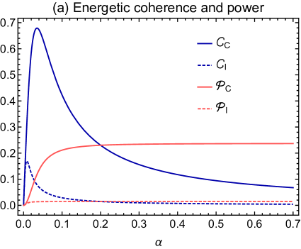
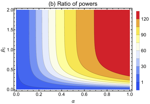
Figure 2: Comparisons of energetic coherence and power outputs in coherent and incoherent engines. The computations are carried out with the parameters $\gamma_{0}=0.01$, $\omega_{h}=10$, $\omega_{c}=5$. (a) The figure on the left illustrates the variation in energetic coherence $\mathcal{C}_{C}=\mathcal{C}(\sigma_{C})$ and $\mathcal{C}_{I}=\mathcal{C}(\sigma_{I})$ for both coherent and incoherent heat engines, respectively with respect to the driving field strength $\alpha$, for $\beta_{h}=0.01$ and $\beta_{c}=0.8$. The expressions of energetic coherence are given Eqs. (7) and (8). The traces in solid-blue and dashed-blue represent $\mathcal{C}_{C}$ and $\mathcal{C}_{I}$, respectively. The corresponding power outputs $\mathcal{P}_{C}$ and $\mathcal{P}_{I}$, given in Eq. (9), by coherent and incoherent engines, are presented with the solid-red and dashed-red traces, respectively. (b) The figure of the right displays the ratio of powers $\mathcal{P}_{C}/\mathcal{P}_{I}=\mathcal{C}_{C}/\mathcal{C}_{I}$ of the coherent and incoherent heat engine, with $\beta_{h}=0.001$, against $\alpha$ and $\beta_{c}$. In fact, for these parameters, the ratio can be $\mathcal{P}_{C}/\mathcal{P}_{I}\geq 135$. See text for more details.

III Quantum enhancements in coherent engines

An evaluation of the performance of a continuous quantum heat engine requires a comprehensive analysis of three metrics: (i) efficiency, which signifies how efficiently heat is being converted into work; (ii) power, which is the rate of work output; and (iii) noise-to-signal ratio (NSR) in power, which signifies the relative fluctuation or inverse of precision in the power output. We compare these metrics for coherent and incoherent heat engines and demonstrate that the former have substantial quantum enhancements in performance over the latter.

Our analysis reveals that the engine performance is related to the energetic coherence present in the steady state $\sigma_{X}$ (for $X=I,C$) in the rotating frame. Henceforth, a steady state refers to the steady state in the rotating frame. The quantum enhancements in the performance of CQHEs over the IQHEs are the direct consequence of the fact that the energetic coherence in $\sigma_{C}$ is higher than that of $\sigma_{I}$, in general. Note that the energetic coherence in the steady state results from a balance between two opposing processes - the (periodic) driving that creates coherence and the dissipation(s) that destroys coherence in the qutrit. Due to coherent heat transfer, the dissipative ‘tendency’ in CQHEs is weaker compared to the dissipative ‘tendency’ in IQHEs. As a result, we observe more energetic coherence in the former.

We start our analysis by studying the coherence in the steady states. In what follows, we set $\gamma_{h}=\gamma_{c}=\gamma_{0}$ and equal driving strength $\alpha$ for fair comparisons. The energetic coherence is measured using the $l$-1 norm of coherence  Baumgratz et al. (2014), given by $\mathcal{C}(\sigma_{X})=\sum_{i\neq j}|\sigma_{X}^{(ij)}|$, where $\sigma_{X}^{(ij)}=\langle i|\sigma_{X}|j\rangle$. For CQHEs and IQHEs, $\sigma_{X}^{(ij)}=\sigma_{X}^{(ji)*}$, and the corresponding amount of energetic coherence in the steady states are given by

$$\mathcal{C}(\sigma_{C}) =\frac{4\alpha\ \gamma_{0}(n_{h}-n_{c})}{8\alpha^{2}+\gamma_{0}^{2}(n_{hc}+2n_{c}n_{h})^{2}},$$ (7)

$$\mathcal{C}(\sigma_{I}) =\frac{4\alpha\ \gamma_{0}(n_{h}-n_{c})}{4\alpha^{2}(3n_{hc}+4)+\gamma_{0}^{2}n_{hc}(n_{hc}+3n_{h}n_{c})},$$ (8)

where $n_{hc}=n_{h}+n_{c}$. We refer to Appendices A and  B for detailed derivation. For fixed $\gamma_{0}$, $n_{h}$, and $n_{c}$, the energetic coherence is a function of the driving strength $\alpha$. As shown in Fig. 2(a), the energetic coherence $\mathcal{C}(\sigma_{C})$ for CQHEs are higher than the energetic coherence $\mathcal{C}(\sigma_{I})$ of IQHEs in general. Even for some reasonable values of system and bath parameters, the $\mathcal{C}(\sigma_{C})$ becomes more than 135 times of $\mathcal{C}(\sigma_{I})$, i.e., $\mathcal{C}(\sigma_{C})\geq 135\ \mathcal{C}(\sigma_{I})$. We also note that, for fixed $n_{h}$, $n_{c}$, and $\gamma_{0}$, there is a critical value of the driving strength $\alpha_{cr}$ for which $\mathcal{C}(\sigma_{C})=\mathcal{C}(\sigma_{I})$. We calculate the critical value (see Appendix C) and observe that $\mathcal{C}(\sigma_{C})\leq\mathcal{C}(\sigma_{I})$ for $\alpha\leq\alpha_{cr}$. However, the $\alpha_{cr}$ is generally very small, representing extremely weak periodic driving, except for the case of the baths with very high temperatures, i.e., $n_{h}\approx n_{c}\gg 1$. In all reasonable physical situations, the engines operate with $\alpha>\alpha_{cr}$, which we consider for evaluating engine performances below.

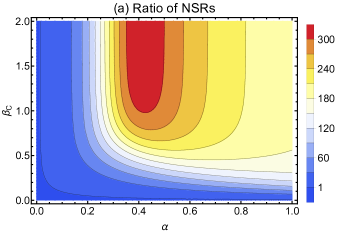
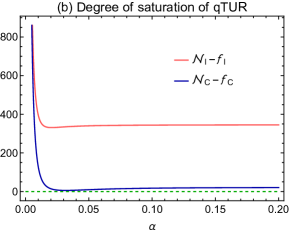
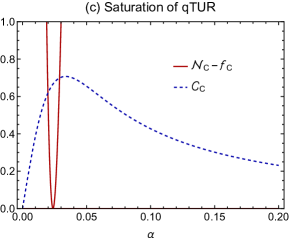
Figure 3: Comparisons of noise-to-signal ratios (NSRs) in coherent and incoherent engines. The parameters $\gamma_{0}=0.01$, $\omega_{h}=10$, and $\omega_{c}=5$ are considered for all the figures. (a) The figure on the left displays the ratio $\mathcal{N}_{I}/\mathcal{N}_{C}$ of NSRs in power (see Eq. (12)) corresponding to incoherent and coherent heat engines against $\beta_{c}$ and $\alpha$, while $\beta_{h}=0.001$. Note, $\mathcal{N}_{I}>\mathcal{N}_{C}$ signifies that the coherent engine produces less NSR in power than the incoherent engine, and the ratio can reach up to $\mathcal{N}_{I}/\mathcal{N}_{C}\geq 330$. (b) The figure in the middle shows the difference between the NSR and its lower bound for CQHEs and IQHEs (i.e., degree of saturation of qTUR) in Eq. (12), involving NSRs and their quantum bounds with respect to $\alpha$ for $\beta_{h}=0.01$ and $\beta_{c}=0.8$. The traces in dark-blue and light-red represent $\mathcal{N}_{C}-f_{C}$ and $\mathcal{N}_{I}-f_{I}$ for the coherent and incoherent engines, respectively. The dashed-green trace corresponds to the zero value. (c) The figure on the right represents the saturation of qTUR by CQHEs for the parameters $\beta_{h}=0.01$ and $\beta_{c}=3$ with a large amount of energetic coherence. Here, $\mathcal{C}_{C}=\mathcal{C}(\sigma_{C})$ represents the energetic coherence in the steady state of CQHEs.

Power and efficiency – Now, we study power and efficiency. The power delivered by a steady state engine has a monotonic relation with the energetic coherence present in the steady state, and it is given by (see Appendices A and  B)

$$\mathcal{P}_{X}=|\langle P_{X}\rangle|=\alpha\ (\omega_{h}-\omega_{c})\ \mathcal{C}(\sigma_{X}),$$ (9)

which is a non-linear function of $\alpha$. As shown in Fig. 2(a), it increases with $\alpha$. The power is proportional to coherence for a given $\alpha$. In fact, the ratio of the powers of CQHEs and IQHEs becomes equal to the ratio of the energetic coherence present in their respective steady states, i.e., $\mathcal{P}_{C}/\mathcal{P}_{I}=\mathcal{C}(\sigma_{C})/\mathcal{C}(\sigma_{I})$. Given that $\mathcal{C}(\sigma_{C})>\mathcal{C}(\sigma_{I})$ in general, the power of CQHEs is higher than the power delivered by IQHEs or $\mathcal{P}_{C}/\mathcal{P}_{I}>1$. A numerical analysis of the power ratio is presented in Fig. 2(b) with respect to the bath temperatures and the driving strength, which displays that not only $\mathcal{P}_{C}/\mathcal{P}_{I}$ is greater than one, but also the ratio may reach more than 135. Clearly, CQHEs exhibit quantum enhancements over IQHEs in power.

The heat current from the hot bath is given by

$$\langle\dot{J}_{X}^{h}\rangle=\alpha\ \omega_{h}\ \mathcal{C}(\sigma_{X}),$$ (10)

for both coherent and incoherent heat engines, and it has a monotonic relation with energetic coherence in the steady states. Yet again, due to energetic coherence, the heat current in CQHEs is higher than in IQHEs. In other words, the CQHEs have a higher capacity to draw heat from the hot bath than the IQHEs. However, the former also produces more power than the latter. Consequently, the efficiency $\eta_{X}=-\langle P_{X}\rangle/\langle\dot{J}_{X}^{h}\rangle$ remains same for both the engines, i.e.,

$$\eta_{I}=\eta_{C}=1-\omega_{c}/\omega_{h}.$$ (11)

Thus, CQHEs perform as good as IQHEs as far as heat-to-work conversion efficiency is concerned. See Appendices A and  D.2 for the derivations.

Noise-to-signal ratio (NSR) in power – In microscopic heat engines, power output often fluctuates. This, in turn, delimits the reliability or stability of the engines. The fluctuation is usually expressed in terms of the variance of power $\Delta P_{X}$, for $X=I,C$. For CQHEs and IQHEs, they are

$$\Delta P_{X}=\lambda_{1}^{X}\langle P_{X}\rangle-\lambda_{2}^{X}\langle P_{X}\rangle^{3},$$

where coefficients $\lambda_{i}^{X}$s are functions of system and bath parameters. See Appendix D for more details.

Ideally, a good engine is expected to deliver high power output and low power output fluctuations. This quality is characterized by the NSR in power, i.e., the ratio between the fluctuation in power $\Delta P_{X}$, and the square of the average power output $\langle P_{X}\rangle^{2}$, and it is lower bounded by a quantum limit Hasegawa (2020) as

$$\mathcal{N}_{X}=\frac{\rm\Delta P_{X}}{\langle P_{X}\rangle^{2}}\geq f_{X},$$ (12)

where the lower bound $f_{X}$ is determined by quantum dynamical activity and coherent dynamical contribution. This relation is known as the quantum thermodynamic uncertainty relation (qTUR), and it is derived using quantum Cramér-Rao bound Hasegawa (2020). The bounds $f_{X}$ in Eq. (12) are different for coherent and incoherent heat engines as they depend on the underlying Markovian dynamics. We find that the $\mathcal{N}_{X}$ depends on the energetic coherence present in the steady states and, for CQHEs and IQHEs, they are (see Appendices D.1 and  D.2)

$$\mathcal{N}_{C} =\frac{F_{p}}{\alpha\ \mathcal{C}(\sigma_{C})}\left(1-\frac{3}{2}\mathcal{C}(\sigma_{C})^{2}\right),$$ (13)

$$\mathcal{N}_{I} =\frac{F_{p}}{\alpha\ \mathcal{C}(\sigma_{I})}\left(1-\frac{k}{F_{p}}\mathcal{C}(\sigma_{I})^{2}\right),$$ (14)

respectively, where

$$F_{p}=\frac{2n_{h}n_{c}+n_{hc}}{n_{h}-n_{c}},\ k=\frac{4\alpha^{2}+\gamma_{0}^{2}(n_{hc}^{2}+2n_{hc}+3n_{h}n_{c})}{\gamma_{0}^{2}(n_{h}-n_{c})}.$$ (15)

From the Eqs. (13) and (14), it is seen that the NSR in both coherent and incoherent engines can be suppressed by accessing energetic coherence in the steady state for fixed $n_{h}$ and $n_{c}$. We observe that the NSR for CQHEs is, in general, much lower than that of IQHEs, which is the consequence of $\mathcal{C}(\sigma_{C})\gg\mathcal{C}(\sigma_{I})$. As shown in Fig. 3(a), the NSR in CQHEs can be as less as 330 times or lower than the NSR attained in IQHEs. Clearly, CQHEs are more reliable or deliver more precision in power than IQHEs.

The saturation of the relation (12), i.e., $\mathcal{N}_{X}=f_{X}$, implies that the engine is producing the least possible NSR in power that is given by its quantum bound. This is the best possible operating condition one would desire from an engine. A numerical analysis presented in Fig. 3(b) demonstrates that the CQHEs can operate in a regime where they yield very low NSR in power close to the quantum bound. In contrast, the IQHE has more NSR in power, which is far from its quantum bound. In addition, the CQHEs can saturate the qTUR by harnessing a large amount of energetic coherence, as shown in Fig. 3(c). Overall, the CQHEs are highly reliable and exhibit substantial quantum enhancements over IQHEs.

Violations of cTUR – For classical heat engines, it is known that the rate of entropy production and the noise-to-signal ratio (NSR) in power follow a trade-off relation. This feature has been studied in terms of classical thermodynamic uncertainty relation (cTUR)  Barato and Seifert (2015), given by

$$\mathcal{Q}=\dot{S}\mathcal{N}\geq 2,$$ (16)

where $\dot{S}=-\beta_{h}\langle\dot{J}_{h}\rangle-\beta_{c}\langle\dot{J}_{c}\rangle$ is the entropy production rate due to steady state dynamics and $\mathcal{N}=\Delta P/\langle P\rangle^{2}$ is NSR in power. It implies that a reduction in NSR can be achieved at the cost of increasing the entropy production rate $\dot{S}$, particularly when the bound in (16) is saturated. This, in turn, represents more degree of irreversibility in the engine operation, leading to a reduced heat-to-work conversion efficiency. A similar conclusion is also drawn from another relation, known as the power-efficiency-constancy trade-off relation Pietzonka and Seifert (2018). Interestingly, it coincides with cTUR for CQHEs and IQHEs (see Appendix E).

We have discussed earlier that, for both coherent and incoherent heat engines, the NSR in power can be reduced while keeping the engine efficiency the same. This is why we witness violations of cTUR by CQHEs and IQHEs for some values of system-bath parameters, signifying that the engines can operate in the quantum regime.

The left-hand side of relation (16) reduces to (for $X=I,C$)

$$\mathcal{Q}_{X}=\ln{\left(\frac{n_{h}(n_{c}+1)}{n_{c}(n_{h}+1)}\right)}F_{X}.$$ (17)

Here $F_{X}=\frac{\Delta\dot{N}_{X}}{\langle\dot{N}_{X}\rangle}$ is the Fano factor, where ${\langle\dot{N}_{X}\rangle}={|\langle P_{X}\rangle}|/(\omega_{h}-\omega_{c})$ is the photon current and ${\Delta\dot{N}_{X}}=\Delta{P}_{X}/(\omega_{h}-\omega_{c})^{2}$ is the fluctuation in photon current. The violation of cTUR by CQHEs and IQHEs implies the violation of $\mathcal{Q}_{C}\geq 2$ and $\mathcal{Q}_{I}\geq 2$, respectively. Interestingly, the corresponding Fano factor can be expressed in terms of energetic coherence as

$$F_{C} =F_{p}\left(1-\frac{3}{2}\mathcal{C}(\sigma_{C})^{2}\right),$$ (18)

$$F_{I} =F_{p}\left(1-\frac{k}{F_{p}}\mathcal{C}(\sigma_{I})^{2}\right),$$ (19)

where $F_{p}$ and $k$ are given in Eq. (15). We refer to Appendix E for the derivations. In the absence of energetic coherence, $\mathcal{Q}=\ln{\left(\frac{n_{h}(n_{c}+1)}{n_{c}(n_{h}+1)}\right)}F_{p}$. In that case, the cTUR is respected because $\ln{\left(\frac{n_{h}(n_{c}+1)}{n_{c}(n_{h}+1)}\right)}F_{p}\geq 2$ Kalaee et al. (2021). On the contrary, for quantum engines, the violations of cTUR can necessarily be attributed to the presence of energetic coherence in the steady states.

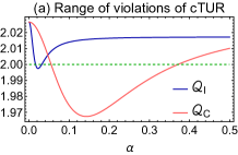
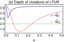
Figure 4: Violations of cTUR by CQHEs and IQHEs. (a) The figure on the left displays the range of violations of cTUR by coherent and incoherent heat engines with respect to $\alpha$, for the parameters $\gamma_{0}=0.01$, $\omega_{h}=10$, $\omega_{c}=5$, $\beta_{h}=0.01$, and $\beta_{c}=0.1$. (b) The figure on the right depicts the depth of violation of cTUR for the parameters $\gamma_{0}=0.01$, $\omega_{h}=10$, $\omega_{c}=5$, $\beta_{h}=0.003$, and $\beta_{c}=0.7$. The figures show that the CQHE violates cTUR for a wider range of parameter $\alpha$. Further, the minimum value of $\mathcal{Q}_{I}$ is $1.997$ while the minimum value of $\mathcal{Q}_{C}$ can be $1.24$. See text for more details.

The important point we highlight here is that the CQHEs violate cTUR not only for a wider range of parameters but also by a higher amount than IQHEs. This is, yet again, due to the fact that $\mathcal{C}(\sigma_{C})>\mathcal{C}(\sigma_{I})$ in general. A numerical study is carried out to compare $\mathcal{Q}_{C}$ and $\mathcal{Q}_{I}$ and presented in Fig. 4(a) and 4(b). We observe that $\mathcal{Q}_{C}$ can have values as low as $1.24$, while the lowest value of $\mathcal{Q}_{I}$ remains very close to $1.997$. Thus, IQHEs only marginally violate the classical limit. Overall, the violations of cTUR for a wider range of parameters and with a larger amount indicate that CQHEs possess more non-classical features than IQHEs.

IV Summary

Recent studies have indicated that the performance of microscopic heat engines can be enhanced by harnessing quantum mechanical features, like energetic quantum coherence. To harness more energetic coherence, we have introduced continuous quantum heat engines that utilize coherent energy (heat) transfers between the working system and the baths via two-photon transitions (Raman transitions). These coherent heat engines are analogous to the traditional Scovil and Schulz-DuBois (SSD) engines, except that the latter only allow incoherent heat transfers via one-photon transitions. The analysis and results presented above clearly demonstrate that, due to coherent heat transfers, coherent heat engines harness much more energetic coherence in the working system than traditional (incoherent) quantum engines. Consequently, the power and noise-to-signal ratio in power is enhanced by hundreds of folds compared to their incoherent analogs. The noise-to-signal ratio in power has a fundamental lower bound derived from the quantum Cramér-Rao bound, and the inequality is termed the quantum thermodynamic uncertainty relation (qTUR). We have shown that coherent engines can yield a substantially low noise-to-signal ratio in power, which is very close to the lower bound (quantum limit). Even the CQHEs can saturate this quantum bound by harnessing high energetic coherence. This suggests that saturation of qTUR requires a high amount of coherence. Thus, coherent engines are highly reliable. In addition, unlike incoherent engines, coherent engines violate classical thermodynamic uncertainty relation for a much wider range of parameters and by a much higher amount. Altogether, the coherent engines possess more quantum features and greatly outperform conventional quantum and classical heat engines, manifesting genuine quantum enhancements.

Two-photon Raman transitions provide a very common and standard tool in contemporary applications of quantum optics (cf. Cohen-Tannoudji et al. (1998); Haroche and Raimond (2006); Meystre and Scully (2021); Larson and Mavrogordatos (2021)). This paves the way for the realization of coherent quantum heat engines on various experimental platforms. Raman transitions have been easily demonstrated in various experimental setups, such as superconducting circuits Aamir et al. (2022); Zanner et al. (2022), atom-optical systems Gauguet et al. (2008); Kristensen et al. (2021), and nitrogen-vacancy centers in diamond Böhm et al. (2021), among others. Thus, our present analysis and results not only improve the understanding of quantum thermal devices, particularly how energetic coherence greatly enhances engine performance, but also open up new avenues for quantum-enabled technologies in the near future.

An executive summary of our main results is below.

• A new model of continuous quantum heat engines is introduced that enables coherent heat transfer between the working system (qutrit) and the baths via two-photon transitions.

• These coherent engines harness a much greater amount of energetic coherence in the qutrit than the analogous incoherent engines, where the latter are the traditional SSD engines.

• The coherent engines yield much higher power and much less signal-to-noise ratio in power compared to incoherent engines, while the efficiency remains the same.

• The coherent engines can operate at or very close to the quantum limit on the noise-to-signal ratio in power imposed by quantum thermodynamic uncertainty relation. Thus, the coherent engines are highly reliable.

• The improvements in performance by coherent engines, exhibiting genuine quantum enhancements, are attributed to the presence of high energetic coherence, which is a consequence of coherent heat transfer.

• The new model of engines with coherent heat transfer and the improved understanding of the role of quantum properties in their performance are expected to find important implications in emerging quantum-enabled technologies.

Appendix A Steady state solution of incoherent quantum heat engines in rotating frame

For incoherent engines, the total Hamiltonian of the qutrit system and two photonic (bosonic) thermal baths can be written as

$$H=H_{S}+H_{B_{h}}+H_{B_{c}}+H_{SB_{h}B_{c}}^{I},$$ (20)

where the Hamiltonian and of the qutrit system is given by

$$H_{S}=\omega_{h}\outerproduct{2}{2}+(\omega_{h}-\omega_{c})\outerproduct{1}{1},$$ (21)

with $\omega_{h}$ and $\omega_{h}-\omega_{c}$ being the frequencies corresponding to the energy gaps. The Hamiltonians of the photonic thermal baths $H_{B_{h}}$ and $H_{B_{c}}$ and the interaction $H_{SB_{h}B_{c}}^{I}$ given in the main text. The corresponding Lindblad master equation describing the local dynamics of the qutrit is given in Eq. (2) in the main text. In a rotating frame, given by $B_{R}=e^{i\tilde{H}t}Be^{-i\tilde{H}t}$ and any operator $B$ and $[H_{0},\tilde{H}]=0$, the master equation becomes

$$\dot{\rho_{R}}= -i[H_{S}-\tilde{H}+H_{dR},\rho_{R}]+\mathcal{D}_{h}(\rho_{R})+\mathcal{D}_{c}(\rho_{R}).$$ (22)

Without loss of generality, we consider $H_{S}=\tilde{H}$. Thus, the steady-state solution of the above master equation can be obtained by solving $\dot{\rho}_{R}=0$ (we denote the steady state by $\sigma_{I}$), and it is

$$\sigma_{I} =\frac{4\alpha^{2}(\gamma_{c}+\gamma_{h}+\gamma_{c}n_{c}+\gamma_{h}n_{h}+\gamma_{c}\gamma_{h}n_{c}(n_{h}+1)(\gamma_{c}n_{c}+\gamma_{h}n_{h})}{4\alpha^{2}(\gamma_{c}(3n_{c}+2)+\gamma_{h}(3n_{h}+2))+\gamma_{c}\gamma_{h}(3n_{c}n_{h}+n_{c}+n_{h})(\gamma_{c}n_{c}+\gamma_{h}n_{h})}\outerproduct{0}{0}$$

$$-\frac{2i\alpha\gamma_{c}\gamma_{h}(n_{h}-n_{c})}{4\alpha^{2}(\gamma_{c}(3n_{c}+2)+\gamma_{h}(3n_{h}+2))+\gamma_{c}\gamma_{h}(3n_{c}n_{h}+n_{c}+n_{h})(\gamma_{c}n_{c}+\gamma_{h}n_{h})}\outerproduct{0}{1}$$

$$+\frac{2i\alpha\gamma_{c}\gamma_{h}(n_{h}-n_{c})}{4\alpha^{2}(\gamma_{c}(3n_{c}+2)+\gamma_{h}(3n_{h}+2))+\gamma_{c}\gamma_{h}(3n_{c}n_{h}+n_{c}+n_{h})(\gamma_{c}n_{c}+\gamma_{h}n_{h})}\outerproduct{1}{0}$$

$$+\frac{4\alpha^{2}(\gamma_{c}+\gamma_{h}+\gamma_{c}n_{c}+\gamma_{h}n_{h}+\gamma_{c}\gamma_{h}n_{h}(n_{c}+1)(\gamma_{c}n_{c}+\gamma_{h}n_{h})}{4\alpha^{2}(\gamma_{c}(3n_{c}+2)+\gamma_{h}(3n_{h}+2))+\gamma_{c}\gamma_{h}(3n_{c}n_{h}+n_{c}+n_{h})(\gamma_{c}n_{c}+\gamma_{h}n_{h})}\outerproduct{1}{1}$$

$$+\frac{(4\alpha^{2}+\gamma_{c}\gamma_{h}n_{c}n_{h})(\gamma_{c}n_{c}+\gamma_{h}n_{h})}{4\alpha^{2}(\gamma_{c}(3n_{c}+2)+\gamma_{h}(3n_{h}+2))+\gamma_{c}\gamma_{h}(3n_{c}n_{h}+n_{c}+n_{h})(\gamma_{c}n_{c}+\gamma_{h}n_{h})}\outerproduct{2}{2}.$$ (23)

The $l$-1 norm of energetic coherence Baumgratz et al. (2014) in the steady state on the rotating frame is

$$\mathcal{C}(\sigma_{I})=|\sigma_{I}^{(01)}|+|\sigma_{I}^{(10)}|=\frac{4\alpha\gamma_{c}\gamma_{h}(n_{h}-n_{c})}{4\alpha^{2}(\gamma_{c}(3n_{c}+2)+\gamma_{h}(3n_{h}+2))+\gamma_{c}\gamma_{h}(3n_{c}n_{h}+n_{c}+n_{h})(\gamma_{c}n_{c}+\gamma_{h}n_{h})},$$ (24)

where $\sigma_{I}^{(ij)}=\langle i|\sigma_{I}|j\rangle$. Now, the average power and the average heat currents in IQHEs corresponding to the hot and cold baths are given by

$$\langle P_{I}\rangle=-i\tr([H_{S},H_{dR}]\sigma_{I})=-i\alpha(\omega_{h}-\omega_{c})(\sigma^{(01)}_{I}-\sigma^{(10)}_{I})=-\alpha(\omega_{h}-\omega_{c})\ \mathcal{C}(\sigma_{I}),$$ (25)

$$\langle\dot{J}^{h}_{I}\rangle=\Tr[\mathcal{D}_{h}(\sigma_{I})H_{S}]=\alpha\ \omega_{h}\ \mathcal{C}(\sigma_{I}),$$ (26)

and $$\langle\dot{J}^{c}_{I}\rangle=\Tr[\mathcal{D}_{c}(\sigma_{I})H_{S}]=-\alpha\ \omega_{c}\ \mathcal{C}(\sigma_{I}),$$ (27)

respectively. Accordingly, the heat-to-work conversion ratio for IQHEs is

$$\eta_{I}=-\frac{\langle P_{I}\rangle}{\langle\dot{J}^{h}_{I}\rangle}=1-\frac{\omega_{c}}{\omega_{h}}.$$ (28)

Appendix B Derivation of Lindblad master equation for coherent quantum heat engines

In this section, we derive the Lindblad master equation for a three-level quantum system coupled with the two photonic (bosonic) thermal baths (hot and cold baths), where the system and baths interact via two-photon transitions (Raman Interactions, i.e., three-body interactions). Our derivation follows the standard textbook approach discussed in Refs. Breuer and Petruccione (2007); Lidar (2020). The total Hamiltonian of the system and two photonic thermal baths can be written as

$$H=H_{S}+H_{B_{h}}+H_{B_{c}}+H_{SB_{h}B_{c}}^{C}.$$ (29)

where suffixes $h$ and $c$ correspond to hot and cold baths, respectively. We assume $\hbar=k_{B}=1$ throughout this work. In Eq. (29), the system Hamiltonian $H_{S}$ describes a three-level system (qutrit), given by

$$H_{S}=\omega_{h}\outerproduct{2}{2}+(\omega_{h}-\omega_{c})b_{hc}^{\dagger}b_{hc}=\omega_{h}\outerproduct{2}{2}+(\omega_{h}-\omega_{c})\outerproduct{1}{1},$$ (30)

where $\omega_{h}$ and $\omega_{h}-\omega_{c}$ refers to the frequencies corresponding to the energy gaps, and $b_{hc}^{\dagger}=|1\rangle\langle 0|$ and $b_{hc}=|0\rangle\langle 1|$. In Eq. (29), the photonic baths are a collection of infinite dimensional systems whose total Hamiltonian is given as

$$H_{B_{h}}+H_{B_{c}}=\sum_{k}\Omega_{k,h}a^{\dagger}_{k,h}a_{k,h}+\sum_{k^{\prime}}\Omega_{k^{\prime},c}a^{\dagger}_{k^{\prime},c}a_{k^{\prime},c}.$$ (31)

Furthermore, in Eq. (29), the interaction Hamiltonian between the system and the baths has the following form Gerry and Eberly (1990); Gerry and Huang (1992); Wu (1996)

$$H_{SB_{h}B_{c}}^{C}=g_{0}\sum_{kk^{\prime}}(a_{k,h}a^{\dagger}_{k^{\prime},c}b_{hc}^{\dagger}+a^{\dagger}_{k,h}a_{k^{\prime},c}b_{hc}),$$ (32)

Here, we consider system-baths coupling to be very weak, i.e., $g_{0}\ll 1$. The total Hamiltonian of the composite system (system + baths) in the interaction picture can be written as

$$\tilde{H}(t)=g_{0}\sum_{k,k^{\prime}}(a_{k,h}(t)a^{\dagger}_{k^{\prime},c}(t)b_{hc}^{\dagger}(t)+a^{\dagger}_{k,h}(t)a_{k^{\prime},c}(t)b_{hc}(t)),$$ (33)

where $b_{hc}(t)=b_{hc}e^{-i(\omega_{h}-\omega_{c})t}$, $b_{hc}^{\dagger}(t)=b_{hc}^{\dagger}e^{i(\omega_{h}-\omega_{c})t}$, $a_{p}(t)=a_{p}e^{-i\omega_{p}t}$ and $a_{p}^{\dagger}(t)=a_{p}^{\dagger}e^{i\omega_{p}t}$. For convenience, we can write the above Hamiltonian

$$\tilde{H}_{I}(t)=g_{0}\sum_{k,k^{\prime}}\sum_{\alpha=\{1,2\}}A_{\alpha}(t)\otimes B_{\alpha,kk^{\prime}}(t),$$ (34)

where $A_{1}(t)=b_{hc}^{\dagger}(t)$, $A_{2}(t)=b_{hc}(t)$, $B_{kk^{\prime},1}(t)=a_{k,h}(t)a^{\dagger}_{k^{\prime},c}(t)$ and $B_{kk^{\prime},2}(t)=a^{\dagger}_{k,h}(t)a_{k^{\prime},c}(t)$. In the interaction picture, the dynamics of the composite system is given by the von Neumann equation,

$$\frac{d\tilde{\rho}(t)}{dt}=-i[\tilde{H}(t),\tilde{\rho}(t)].$$ (35)

For the cases where the system and baths are initially in a product state and very weakly coupled, using Born and Markov approximations, we obtain the following dynamical equation of the system

$$\frac{d\tilde{\rho}(t)}{dt}=-g_{0}^{2}\sum_{\alpha\beta}\sum_{kk^{\prime}ss^{\prime}}\int_{0}^{\infty}d\tau\{\mathcal{B}_{\alpha\beta,kk^{\prime}ss^{\prime}}(\tau,0)[A_{\alpha}(t),A_{\beta}(t-\tau)\tilde{\rho}(t)]+\mathcal{B}_{\beta\alpha,ss^{\prime}kk^{\prime}}(0,\tau)[\tilde{\rho}(t)A_{\beta}(t-\tau),A_{\alpha}(t)]\},$$ (36)

where $\mathcal{B}_{\alpha\beta,kk^{\prime}ss^{\prime}}(\tau,0)=\tr(e^{iH_{B}\tau}B_{\alpha,kk^{\prime}}e^{-iH_{B}\tau}B_{\beta,ss^{\prime}}\rho_{\beta_{h}}\otimes\rho_{\beta_{c}})$ and $\mathcal{B}_{\beta\alpha,ss^{\prime}kk^{\prime}}(0,\tau)=\tr(B_{\beta,ss^{\prime}}e^{iH_{B}\tau}B_{\alpha,kk^{\prime}}e^{-iH_{B}\tau}\rho_{\beta_{h}}\otimes\rho_{\beta_{c}})$. Here $H_{B}=H_{B_{h}}+H_{B_{c}}$ is total free Hamiltonian of the baths. The states $\rho_{\beta_{h}}$ and $\rho_{\beta_{c}}$ are the thermal states of hot and cold baths at inverse temperatures $\beta_{h}$ and $\beta_{c}$. The above dynamical equation in the frequency domain can be written as

$$\frac{d\tilde{\rho}(t)}{dt}=-g_{0}^{2}\sum_{kk^{\prime}ss^{\prime}} \big{[}\int_{0}^{\infty}d\tau\mathcal{B}_{12,kk^{\prime}ss^{\prime}}(\tau,0)e^{i\omega_{hc}\tau}[b_{hc}^{\dagger},b_{hc}\tilde{\rho}(t)]+\int_{0}^{\infty}d\tau\mathcal{B}_{21,kk^{\prime}ss^{\prime}}(\tau,0)e^{-i\omega_{hc}\tau}[b_{hc},b_{hc}^{\dagger}\tilde{\rho}(t)]$$

$$+\int_{0}^{\infty}d\tau\mathcal{B}_{12,kk^{\prime}ss^{\prime}}(0,\tau)e^{-i\omega_{hc}\tau}[\tilde{\rho}(t)b_{hc}^{\dagger},b_{hc}]+\int_{0}^{\infty}d\tau\mathcal{B}_{21,kk^{\prime}ss^{\prime}}(0,\tau)e^{i\omega_{hc}\tau}[\tilde{\rho}(t)b_{hc},b_{hc}^{\dagger}]\big{]},$$ (37)

where $\omega_{hc}=\omega_{h}-\omega_{c}$. The bath correlation functions can be simplified as

$$\sum_{kk^{\prime}ss^{\prime}}\int_{0}^{\infty}d\tau\mathcal{B}_{12}(\tau,0)e^{i\omega_{hc}\tau}=\sum_{kk^{\prime}ss^{\prime}}\int_{0}^{\infty}d\tau\langle a_{k,h}(\tau)a^{\dagger}_{k^{\prime},c}(\tau)a^{\dagger}_{s,h}a_{s^{\prime},c}\rangle e^{i\omega_{hc}\tau}=\sum_{kk^{\prime}}(n_{k,h}(\Omega_{k,h})+1)n_{k^{\prime},c}(\Omega_{k^{\prime},c})\int_{0}^{\infty}d\tau e^{-i(\Delta_{kk^{\prime},hc}-\omega_{hc})\tau},$$

$$\sum_{kk^{\prime}ss^{\prime}}\int_{0}^{\infty}d\tau\mathcal{B}_{21}(\tau,0)e^{-i\omega_{hc}\tau}=\sum_{kk^{\prime}}(n_{k,c}(\Omega_{k,h})+1)n_{k^{\prime},h}(\Omega_{k^{\prime},c})\int_{0}^{\infty}d\tau e^{i(\Delta_{kk^{\prime},hc}-\omega_{hc})\tau},$$

$$\sum_{kk^{\prime}ss^{\prime}}\int_{0}^{\infty}d\tau\mathcal{B}_{12}(0,\tau)e^{-i\omega_{hc}\tau}=\sum_{kk^{\prime}}(n_{k,h}(\Omega_{k,h})+1)n_{k^{\prime},c}(\Omega_{k^{\prime},c})\int_{0}^{\infty}d\tau e^{i(\Delta_{hc}-\omega_{kk^{\prime},hc})\tau},$$

$$\sum_{kk^{\prime}ss^{\prime}}\int_{0}^{\infty}d\tau\mathcal{B}_{21}(\tau,0)e^{-i\omega_{hc}\tau}=\sum_{kk^{\prime}}(n_{k,c}(\Omega_{k,h})+1)n_{k^{\prime},c}(\Omega_{k^{\prime},h})\int_{0}^{\infty}d\tau e^{-i(\Delta_{kk^{\prime},hc}-\omega_{hc})\tau},$$

$$\sum_{kk^{\prime}ss^{\prime}}\int_{0}^{\infty}d\tau e^{\pm i(\Delta_{kk^{\prime},hc}-\omega_{hc})\tau}=\sum_{kk^{\prime}}\pi\delta(\Delta_{kk^{\prime},hc}-\omega_{hc})\pm i\mathbb{P}(\frac{1}{\Delta_{kk^{\prime},hc}-\omega_{hc}}),$$

where $\Delta_{kk^{\prime},hc}=\Omega_{k,h}-\Omega_{k^{\prime},c}$. Here we have used the relations $\langle a^{\dagger}_{p}a_{p^{\prime}}\rangle=n_{p}\delta_{pp^{\prime}}$, $\langle a_{p}a^{\dagger}_{p^{\prime}}\rangle=(n_{p}+1)\delta_{pp^{\prime}}$ and $\langle a_{p}a_{p^{\prime}}\rangle=\langle a^{\dagger}_{p}a^{\dagger}_{p}\rangle=0$ to simplify the bath correlation functions. To further simplify these functions, now we also convert $\sum_{p}\sum_{p^{\prime}}=\int_{0}^{\infty}\int_{0}^{\infty}d\Omega d\Omega^{\prime}D(\Omega)D(\Omega^{\prime})$, where $D(\Omega)$ is the photon density of states, i.e. the number of photon modes in a small frequency interval $[\Omega,\Omega+d\Omega]$. Ignoring the principal value part for the moment, we then obtain

$$\sum_{k,k^{\prime}}f \left(n_{h}(\Omega_{k,h}),n_{c}(\Omega_{k^{\prime},c})\right)\int_{0}^{\infty}d\tau e^{\pm i(\Delta_{kk^{\prime},hc}-\omega_{hc})\tau}$$

$$=\pi\int_{0}^{\infty}d\Omega_{h}D(\Omega_{h})\int_{0}^{\infty}d\Omega_{c}D(\Omega_{c})f\left(n_{h}(\Omega_{h}),n_{c}(\Omega_{c})\right)\delta\left((\Omega_{h}-\Omega_{c})-(\omega_{h}-\omega_{c})\right),$$ (38)

where $f$ is a function of $n_{h}(\Omega_{k,h})$ and $n_{c}(\Omega_{k^{\prime},c})$. The double integral on the right-hand side is correlated. To match it with the incoherent quantum heat engines case, we enforce the resonance condition $(\Omega_{c}=\omega_{c})$ and $(\Omega_{h}=\omega_{h})$. As a consequence, the expression reduces to

$$\sum_{k,k^{\prime}}f(n_{h}(\Omega_{k,h}),n_{c}(\Omega_{k^{\prime},c}))\int_{0}^{\infty}d\tau e^{\pm i(\Delta_{kk^{\prime},hc}-\omega_{hc})\tau}=\pi\int_{0}^{\infty}d\Omega_{h}D(\Omega_{h})\int_{0}^{\infty}d\Omega_{c}D(\Omega_{c})f(n_{h}(\Omega_{h}),n_{c}(\Omega_{c}))\delta(\Omega_{h}-\omega_{h})\delta(\Omega_{c}-\omega_{c}),$$ (39)

and finally to

$$\sum_{k,k^{\prime}}f(n_{h}(\Omega_{k,h}),n_{c}(\Omega_{k^{\prime},c}))\int_{0}^{\infty}d\tau e^{\pm i(\Delta_{kk^{\prime},hc}-\omega_{hc})\tau}=\pi f(n_{h}(\omega_{h}),n_{c}(\omega_{c}))D(\omega_{c})D(\omega_{h}).$$ (40)

After substituting the expression of simplified bath correlation functions in Eq. (B), we obtain the Lindblad master equation

$$\frac{d\tilde{\rho}(t)}{dt}=\gamma_{1}\left(b_{hc}\tilde{\rho}(t)b_{hc}^{\dagger}-\frac{1}{2}\{b_{hc}^{\dagger}b_{hc},\tilde{\rho}(t)\}\right)+\gamma_{2}\left(b_{hc}^{\dagger}\tilde{\rho}(t)b_{hc}-\frac{1}{2}\{b_{hc}b_{hc}^{\dagger},\tilde{\rho}(t)\}\right),$$

where $\gamma_{1}=\gamma_{0}n_{c}(n_{h}+1)$, $\gamma_{2}=\gamma_{0}n_{h}(n_{c}+1)$, $\gamma_{0}=2g_{0}^{2}\pi D(\omega_{c})D(\omega_{h})$ is Weiskopf-Wigner decay constant, and $n_{x}=1/(e^{\beta_{x}\omega_{x}}-1)$ is average boson number of the bath ’$x$’ with inverse temperature $\beta_{x}$ ($x=h,c$). The Lindblad master equation derived above is in the interaction picture. It can be expressed in Schrodinger’s Picture as

$$\frac{d{\rho}(t)}{dt} =-i[H_{S},\rho(t)]+\gamma_{1}\left(b_{hc}{\rho}(t)b_{hc}^{\dagger}-\frac{1}{2}\{b_{hc}^{\dagger}b_{hc},{\rho}(t)\}\right)+\gamma_{2}\left(b_{hc}^{\dagger}{\rho}(t)b_{hc}-\frac{1}{2}\{b_{hc}b_{hc}^{\dagger},{\rho}(t)\}\right).$$

This dynamics leads to a steady state $\rho_{ss}$, i.e., $\dot{\rho}_{ss}=0$, given by

$$\rho_{ss}=\frac{\text{$\gamma$}_{1}}{(\text{$\gamma$}_{1}+\text{$\gamma$}_{2})}\outerproduct{0}{0}+\frac{\text{$\gamma$}_{2}}{(\text{$\gamma$}_{1}+\text{$\gamma$}_{2})}\outerproduct{1}{1}.$$ (41)

For the steady state, the ratio of populations of exited state $|1\rangle$ and ground state $|0\rangle$ is given as

$$\frac{\rho^{(11)}_{ss}}{\rho^{(00)}_{ss}}=\frac{\gamma_{2}}{\gamma_{1}}=e^{{-(\beta_{h}\omega_{h}-\beta_{c}\omega_{c})}}=e^{-\frac{(\beta_{h}\omega_{h}-\beta_{c}\omega_{c})}{(\omega_{h}-\omega_{c})}(\omega_{h}-\omega_{c})},$$ (42)

where $\rho^{(ij)}_{ss}=\langle i|\rho_{ss}|j\rangle$. To have an engine operation by utilizing two-photon transitions, we need population inversion, i.e., $\frac{\rho^{(11)}_{ss}}{\rho^{(00)}_{ss}}>1$. For this, the required condition is $\beta_{h}\omega_{h}-\beta_{c}\omega_{c}<0$. This also implies $n_{h}>n_{c}$.

B.1 Steady state solution of coherent quantum heat engines in rotating frame

With an external periodic driving on the qutrit $H_{d}(t)=\alpha(e^{-i\omega t}|1\rangle\langle 0|+e^{i\omega t}|0\rangle\langle 1|)$, the Lindblad master equation describing the dynamics of a coherent quantum heat engine becomes

$$\dot{\rho}= -i[H_{S}+H_{d}(t),\rho]+\mathcal{D}_{hc}(\rho),$$ (43)

where the master equation involves single dissipator $\mathcal{D}_{hc}(\rho)$, given by

$$\mathcal{D}_{hc}(\rho)=\gamma_{1}(b_{hc}{\rho}(t)b_{hc}^{\dagger}-\frac{1}{2}\{b_{hc}^{\dagger}b_{hc},{\rho}(t)\})+\gamma_{2}(b_{hc}^{\dagger}{\rho}(t)b_{hc}-\frac{1}{2}\{b_{hc}b_{hc}^{\dagger},{\rho}(t)\}).$$ (44)

We can transform the above Lindblad master equation to the rotating frame using the transformation $B_{R}=e^{i\tilde{H}t}Be^{-i\tilde{H}t}$, where $B$ is an arbitrary operator and $[H_{S},\tilde{H}]=0$, as follows:

$$\dot{\rho}_{R}= -i[H_{S}-\tilde{H}+H_{dR},\rho_{R}]+\mathcal{D}_{hc}(\rho_{R}),$$ (45)

where $H_{dR}$ corresponds the driving Hamiltonian $H_{d}(t)$ in rotating frame. Without loss of generality, we consider $H_{S}=\tilde{H}$.

A steady-state solution of the above master equation can be obtained by solving $\dot{\rho}_{R}=0$ (we denote the steady state by $\sigma_{C}$), which yields

$$\sigma_{C}=\frac{4\alpha^{2}+\gamma_{1}(\gamma_{1}+\gamma_{2})}{8\alpha^{2}+(\gamma_{1}+\gamma_{2})^{2}}\outerproduct{0}{0}+\frac{2i\alpha(\gamma_{1}-\gamma_{2})}{8\alpha^{2}+(\gamma_{1}+\gamma_{2})^{2}}\outerproduct{0}{1}\\ -\frac{2i\alpha(\gamma_{1}-\gamma_{2})}{8\alpha^{2}+(\gamma_{1}+\gamma_{2})^{2}}\outerproduct{1}{0}+\frac{4\alpha^{2}+\gamma_{2}(\gamma_{1}+\gamma_{2})}{8\alpha^{2}+(\gamma_{1}+\gamma_{2})^{2}}\outerproduct{1}{1}.$$ (46)

The $l$-1 norm of coherence Baumgratz et al. (2014) of the steady state in CQHEs can be expressed as

$$\mathcal{C}(\sigma_{C})=|\sigma_{C}^{(01)}|+|\sigma_{C}^{(10)}|=\frac{4\gamma_{0}\alpha(n_{h}-n_{c})}{8\alpha^{2}+\gamma_{0}^{2}(2n_{h}n_{c}+n_{h}+n_{c})^{2}},$$ (47)

where $\sigma_{C}^{(ij)}=\langle i|\sigma_{I}|j\rangle$. The average power is directly related to energetic coherence as

$$\langle P_{C}\rangle=-i\tr([H_{S},H_{dR}]\sigma_{C})=-i\alpha(\omega_{h}-\omega_{c})(\sigma^{(01)}_{C}-\sigma^{(10)}_{C})=-\alpha(\omega_{h}-\omega_{c})\ \mathcal{C}(\sigma_{C}).$$ (48)

The dynamics due to heat transfer with the baths is governed by single dissipator $\mathcal{D}_{hc}$, unlike in IQHEs discussed in Appendix A, and it takes into account the contributions from hot and cold baths together. Because of that, we cannot directly calculate the heat currents from the hot and cold baths with the dissipator. We overcome this limitation by employing the full counting statistics (FCS) of the steady-state dynamics in the rotating frame (see Appendix D).

Appendix C Comparison of energetic coherences in coherent and incoherent heat engines

The energetic coherence in the steady state of the qutrit is non-linearly dependent on the driving parameter $\alpha$ for both coherent and incoherent heat engines. It is, in general, higher in the coherent heat engines compared to the incoherent ones. However, for some values of $\alpha$, the energetic coherence in the coherent heat engines can be lower than the incoherent ones. The driving parameter has a critical value, given by $\alpha_{cr}$, below which the energetic coherence is higher for incoherent heat engines. We determine the $\alpha_{cr}$ by solving the condition

$$\mathcal{C}(\sigma_{C})=\mathcal{C}(\sigma_{I}),$$ (49)

and it is

$$\alpha_{cr}=\gamma_{0}\sqrt{\frac{(n_{h}+n_{c})(n_{h}+n_{c}+3n_{h}n_{c})-\gamma_{0}^{2}(n_{c}+n_{h}+2n_{c}n_{h})^{2}}{8-4\left(3(n_{h}+n_{c})+4\right)}}.$$ (50)

The $\mathcal{C}(\sigma_{C})>\mathcal{C}(\sigma_{I})$ for $\alpha>\alpha_{cr}$ and $\mathcal{C}(\sigma_{C})\leq\mathcal{C}(\sigma_{I})$ for $\alpha\leq\alpha_{cr}$. Note that we need to satisfy the condition $n_{h}>n_{c}$ for the continuous device to operate as a heat engine. However, for reasonable values of the parameters $n_{h}$, $n_{c}$, and $\gamma_{0}$, the critical value $\alpha_{cr}$ remains very small, corresponding to a very weak external driving. Fig. 5 illustrates how $\alpha_{cr}$ varies with respect to inverse temperatures of the baths. In the exceptional cases where the baths are extremely hot, i.e., $n_{h}\approx n_{c}\gg 1$, the $\alpha_{cr}$ becomes very high. Nevertheless, considering the usual experimental situations, the engines operate with $\alpha>\alpha_{cr}$, and the coherent engines yield more energetic coherence in their steady state than the incoherent engines.

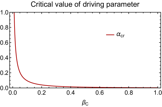
Figure 5: The figure depicts the variation of the critical value of the driving parameter against the inverse temperature of the cold bath. Here we consider $\gamma_{0}$ = 0.01, $\omega_{h}$ = 10, $\omega_{c}$ = 5, and $\beta_{h}$ = 0.001.

Appendix D Full Counting Statistics

Full Counting Statistics (FCS) provides an analytical approach to determine the statistics of the quantity of interests $M$, such as power, currents corresponding to each bath, and their fluctuations in an open quantum system dynamics Esposito et al. (2009). This approach incorporates counting fields into the master equation. Suppose $\rho(\chi,t)$ represents the solution of the dressed Lindblad master equation. In that case, we define the moment-generating function $\mathcal{M}(\chi,t)$ and the cumulant-generating function $\mathcal{F}(\chi,t)$ as follows:

$$\mathcal{M}(\chi,t)=\mathrm{tr}{\{\rho(\chi,t)\}},\ \mbox{and}\ \mathcal{F}(\chi,t)=\ln\mathcal{M}(\chi,t).$$ (51)

Sometimes, a description in terms of cumulants is more convenient. The advantage lies in the fact that the dominant eigenvalue of the Liouvillian usually determines the long-time evolution of the cumulant-generating function:

$$\mathcal{C}(\chi,t)\approx\lambda(\chi)t,$$ (52)

where $\lambda(\chi)$is the eigenvalue of $\mathcal{L}(\chi)=\mathcal{L}(\chi,0)$ with the largest real part (uniqueness assumed) and it vanishes when $\chi=0$.

In the long-time limit, the cumulants of the quantity of interest $M$ in the steady state can be obtained using the following formula:

$$\langle\langle M^{k}\rangle\rangle=\bigg{(}\frac{d}{d(i\chi)}\bigg{)}^{k}\lambda(\chi)\bigg{|}_{\chi=0}.$$ (53)

The first and second cumulants correspond to the mean and variance of the quantity of interest $M$, respectively:

$$\langle M\rangle=\bigg{(}\frac{d}{d(i\chi)}\bigg{)}\lambda(\chi)\bigg{|}_{\chi=0},\ \ \mbox{and}\ \ \Delta M=\langle\langle M^{2}\rangle\rangle=\bigg{(}\frac{d}{d(i\chi)}\bigg{)}^{2}\lambda(\chi)\bigg{|}_{\chi=0}.$$ (54)

A direct computation of $\lambda(\chi)$ is not straightforward. To analytically determine the mean and variance from the derivatives, we follow the method outlined in Refs. Bruderer et al. (2014); Kalaee et al. (2021); Prech et al. (2023); Landi et al. (2024). Consider the characteristic polynomial of $\cal{L}(\chi)$

$$\sum_{n}a_{n}\lambda(\chi)^{n}=0,$$ (55)

where the terms $a_{n}$ are functions of $\chi$. Derivatives of $a_{n}$ are defined as

$$a^{\prime}_{n}=i\frac{d}{d\chi}a_{n}|_{\chi=0},\ \mbox{and}\ a^{\prime\prime}_{n}=\big{(}i\frac{d}{d\chi}\big{)}^{n}a_{n}|_{\chi=0}.$$ (56)

With a little analysis, we can express mean and variance as (for more details, see appendices of Refs. Kalaee et al. (2021); Prech et al. (2023); Landi et al. (2024)):

$$\langle M\rangle=-\frac{a^{\prime}_{0}}{a_{1}},\ \mbox{and}\ \Delta M=\bigg{(}\frac{a^{\prime\prime}_{0}}{a^{\prime}_{0}}-\frac{2a^{\prime}_{1}}{a_{1}}\bigg{)}\langle M\rangle-\frac{2a_{2}}{a_{1}}\langle M\rangle^{2}.$$ (57)

Note that the above expressions of mean and variance hold for all systems with Lindblad dynamics with a unique steady state.

D.1 Counting field statistics for coherent quantum heat engines

Here, we re-derive the Lindblad master equation of coherent heat engine by introducing counting fields, which will help us to evaluate current and power statistics Esposito et al. (2009). The total Hamiltonian for the system and the baths (in the presence of driving) is given as

$$H=H_{S}+H_{d}(t)+H_{B_{h}}+H_{B_{c}}+H_{SB_{h}B_{c}}^{C}.$$ (58)

where $H_{d}(t)$ represents the external driving field acting on the three-level system and the rest of the Hamiltonians defined in the previous section. Here, we are considering a situation where the two baths continuously interact with the system, and the interaction between the system and the baths is weak. We choose the initial state as a product state, i.e., $\rho(0)=\rho_{S}(0)\otimes\rho_{B}$, where $\rho_{B}=\rho_{\beta_{h}}\otimes\rho_{\beta_{c}}$ and the baths are prepared in thermal states with respective Hamiltonians $H_{B_{h}}$, $H_{B_{c}}$ and inverse temperatures $\beta_{h}$ and $\beta_{c}$, respectively. To measure the observables are the Hamiltonians $H_{B_{h}}$ and $H_{B_{c}}$ and to get the corresponding probability distributions of their measurement, we introduce counting field $\chi_{j}$ $(j=h,c)$ to each bath. We introduce $\chi\equiv{\{\chi_{h},\chi_{c}\}}$ to denote collectively both the counting variables. The modified density matrix $\rho(\chi,t)$ of composite system is given as

$$\rho(\chi,t)=U(\chi,t)\rho(0)\bar{U}(-\chi,t),$$ (59)

with

$$U(\chi,t)=e^{-i(\chi_{h}H_{B_{h}}+\chi_{c}H_{B_{c}})/2}U(t)e^{i(\chi_{h}H_{B_{h}}+\chi_{c}H_{B_{c}})/2}\ \ \mbox{and}\ \ \bar{U}(-\chi,t)=e^{i(\chi_{h}H_{B_{h}}+\chi_{c}H_{B_{c}})/2}U^{\dagger}(t)e^{-i(\chi_{h}H_{B_{h}}+\chi_{c}H_{B_{c}})/2}$$

being the counting field-dressed evolution operator. Here $U(t)$ is the unitary evolution operator generated by the total Hamiltonian $H$. The time evolution of modified density matrix $\rho(\chi,t)$ is given by following master equation

$$\frac{d\rho(\chi,t)}{dt}=-i[H(\chi,t)\rho(\chi,t)-\rho(\chi,t)H(-\chi,t)],$$ (60)

where, $H(\chi,t)=e^{-i(\chi_{h}H_{B_{h}}+\chi_{c}H_{B_{c}})/2}He^{i(\chi_{h}H_{B_{h}}+\chi_{c}H_{B_{c}})/2}$. In the interaction picture, one gets (the operators are labeled by tilde)

$$\tilde{\rho}(\chi,t)=U_{0}\rho(\chi,t)U^{\dagger}_{0},$$ (61)

where $U_{0}$ is the unitary operator generated by the Hamiltonian $H_{0}(t)=H_{S}(t)+H_{B}$. Here we have denoted $H_{S}(t)=H_{S}+H_{d}(t)$ and $H_{B}=H_{B_{h}}+H_{B_{c}}$. In the interaction picture, the dressed total Hamiltonian is given by

$$\tilde{H}_{I}(\chi,t)=U_{0}H_{SB}(\chi,t)U_{0}^{\dagger}=\sum_{\alpha,kk^{\prime}}A_{\alpha}(t)\otimes B_{\alpha,kk^{\prime}}(\chi,t)\ \ \mbox{and}\ \ \tilde{H}_{I}(-\chi,t)=U_{0}H_{SB}(\chi,t)U_{0}^{\dagger}=\sum_{\alpha,kk^{\prime}}A_{\alpha}(t)\otimes B_{\alpha,kk^{\prime}}(-\chi,t),$$ (62)

where $B_{\alpha,kk^{\prime}}(\chi,t)=B^{h}_{\alpha,k}(\chi_{h},t)\otimes B^{c}_{\alpha,k^{\prime}}(\chi_{c},t)$ and $B^{h(c)}$’s are bath operators corresponding to hot (cold) bath. In the interaction picture, the evolution equation can be written as

$$\frac{d\tilde{\rho}(\chi,t)}{dt}=-i[\tilde{H}_{I}(\chi,t)\tilde{\rho}(\chi,t)-\tilde{\rho}(\chi,t)\tilde{H}_{I}(-\chi,t)].$$ (63)

Next, considering the weak coupling assumption and performing the standard Born-Markov approximation, we arrive at the following master equation

$$\frac{d\tilde{\rho}_{S}(\chi,t)}{dt}=-\int_{0}^{\infty}d\tau{\rm Tr}_{B}[\tilde{H}_{I} (\chi,t)\tilde{H}_{I}(\chi,t-\tau)\tilde{\rho}_{S}(\chi,t)\rho_{B}-\tilde{H}_{I}(\chi,t)\tilde{\rho}_{S}(\chi,t)\rho_{B}\tilde{H}_{I}(-\chi,t-\tau)$$

$$-\tilde{H}_{I}(\chi,t-\tau)\tilde{\rho}_{S}(\chi,t)\rho_{B}\tilde{H}_{I}(-\chi,t)+\tilde{\rho}_{S}(\chi,t)\rho_{B}\tilde{H}_{I}(-\chi,t-\tau)\tilde{H}_{I}(-\chi,t)],$$ (64)

where we have used ${\rm Tr}_{B}[\tilde{H}_{I}(\chi,t)\ \rho_{B}]=0$, and $\rho_{B}=\rho_{\beta_{h}}\otimes\rho_{\beta_{c}}$. After simplification, the above equation can be written as

$$\frac{d\tilde{\rho}_{S}(\chi,t)}{dt}=-g_{0}^{2}\int_{0}^{\infty}d\tau\sum_{\alpha\beta kk^{\prime}ss^{\prime}} \left({A}_{\alpha}(t){A}_{\beta}(t-\tau)\tilde{\rho}_{S}(\chi,t)\Tr[{B}_{\alpha,kk^{\prime}}(\chi,t){B}_{\beta,ss^{\prime}}(\chi,t-\tau)\rho_{B}]\right.$$

$$-{A}_{\alpha}(t)\tilde{\rho}_{S}(\chi,t){A}_{\beta}(t-\tau)\Tr[{B}_{\alpha,kk^{\prime}}(\chi,t)\rho_{B}{B}_{\beta,ss^{\prime}}(-\chi,t-\tau)]$$

$$-{A}_{\alpha}(t-\tau)\tilde{\rho}_{S}(\chi,t){A}_{\beta}(t)\Tr[{B}_{\alpha,kk^{\prime}}(\chi,t-\tau)\rho_{B}{B}_{\beta,ss^{\prime}}(-\chi,t)]$$

$$\left.+\tilde{\rho}_{S}(\chi,t){A}_{\alpha}(t-\tau){A}_{\beta}(t)\Tr[\rho_{B}{B}_{\alpha,kk^{\prime}}(-\chi,t-\tau){B}_{\beta,ss^{\prime}}(-\chi,t)]\right).$$

After further simplifying the bath correlation function, we obtain

$$\frac{d\tilde{\rho}_{S}(\chi,t)}{dt}= -g_{0}^{2}\int_{0}^{\infty}d\tau\sum_{\alpha\beta}\sum_{kk^{\prime}ss^{\prime}}({A}_{\alpha}(t){A}_{\beta}(t-\tau)\tilde{\rho}_{S}(\chi,t)\tr[{B}_{\alpha,kk^{\prime}}(\tau){B}_{\beta,ss^{\prime}}(0)\rho_{B}]-{A}_{\alpha}(t)\tilde{\rho}_{S}(\chi,t){A}_{\beta}(t-\tau)\tr[{B}_{\beta,ss^{\prime}}(-2\chi,\tau){B}_{\alpha,kk^{\prime}}(0)\rho_{B}]$$

$$-{A}_{\alpha}(t-\tau)\tilde{\rho}_{S}(\chi,t){A}_{\beta}(t)\tr[{B}_{\beta,ss^{\prime}}(-2\chi,t){B}_{\alpha,kk^{\prime}}(0)\rho_{B}]+\tilde{\rho}_{S}(\chi,t){A}_{\alpha}(t-\tau){A}_{\beta}(t)\tr[{B}_{\alpha,kk^{\prime}}(-\tau){B}_{\beta,ss^{\prime}}(0)\rho_{B}]).$$

Using the explicit form of system and bath operators $A_{1}(t)=b_{hc}^{\dagger}(t)$, $A_{2}(t)=b_{hc}(t)$, $B_{kk^{\prime},1}(t)=a_{k,h}(t)a^{\dagger}_{k^{\prime},c}(t)$, $B_{kk^{\prime},2}(t)=a^{\dagger}_{k,h}(t)a_{k^{\prime},c}(t)$, $b_{hc}(t)=b_{hc}e^{-i(\omega_{h}-\omega_{c})t}$, $b_{hc}^{\dagger}(t)=b_{hc}^{\dagger}e^{i(\omega_{h}-\omega_{c})t}$, $a_{p}(t)=a_{p}e^{-i\omega_{p}t}$ and $a_{p}^{\dagger}(t)=a_{p}^{\dagger}e^{i\omega_{p}t}$, and solving the bath correlation function and converting sums into integrals as considered in the previous section B, we get the following dressed Lindblad master equation in Schrodinger picture as

$$\frac{d{\rho}(\chi,t)}{dt}=-i[H_{S}+H_{d}(t),\rho]+\gamma_{1}(e^{i(\omega_{h}\chi_{h}-\omega_{c}\chi_{c})}b_{hc}{\rho}(t)b_{hc}^{\dagger}-\frac{1}{2}\{b_{hc}^{\dagger}b_{hc},{\rho}(t)\})+\gamma_{2}(e^{-i(\omega_{h}\chi_{h}-\omega_{c}\chi_{c})}b_{hc}^{\dagger}{\rho}(t)b_{hc}-\frac{1}{2}\{b_{hc}b_{hc}^{\dagger},{\rho}(t)\}),$$ (65)

where $\gamma_{1}=\gamma_{0}n_{c}(n_{h}+1)$, $\gamma_{2}=\gamma_{0}n_{h}(n_{c}+1)$, $\gamma_{0}=2g^{2}\pi D(\omega_{c})D(\omega_{h})$ is Weiskopf-Wigner decay constant, and $n_{x}=1/(e^{\beta_{x}\omega_{x}}-1)$ is the average photon number in the bath with inverse temperature $\beta_{x}$. In the rotating frame, the above master equation reduces to

$$\frac{d{\rho}(\chi,t)}{dt}=-i[H_{dR},\rho]+\gamma_{1}(e^{i(\omega_{h}\chi_{h}-\omega_{c}\chi_{c})}b_{hc}{\rho}(t)b_{hc}^{\dagger}-\frac{1}{2}\{b_{hc}^{\dagger}b_{hc},{\rho}(t)\})+\gamma_{2}(e^{-i(\omega_{h}\chi_{h}-\omega_{c}\chi_{c})}b_{hc}^{\dagger}{\rho}(t)b_{hc}-\frac{1}{2}\{b_{hc}b_{hc}^{\dagger},{\rho}(t)\}),$$ (66)

and the corresponding full Liouvillian super-operator with counting fields is

$$\mathcal{L}(\chi_{h},\chi_{c})=\left(\begin{array}[]{cccc}-\text{$\gamma$}_{1}&-i\alpha&i\alpha&\text{$\gamma$}_{2}e^{-i(\chi_{h}\text{$\omega$}_{h}-\chi_{c}\text{$\omega$}_{c})}\\ -i\alpha&-\frac{\text{$\gamma$}_{1}}{2}-\frac{\text{$\gamma$}_{2}}{2}&0&i\alpha\\ i\alpha&0&-\frac{\gamma_{1}}{2}-\frac{\text{$\gamma$}_{2}}{2}&-i\alpha\\ \text{$\gamma$}_{1}e^{i(\chi_{h}\text{$\omega$}_{h}-\chi_{c}\text{$\omega$}_{c})}&i\alpha&-i\alpha&-\text{$\gamma$}_{2}\\ \end{array}\right).$$ (67)

For calculating power statistics, we set $\chi_{h}=\chi_{c}=\chi$. Following the previous discussion in this section, we can determine the polynomial factors with respective derivatives

$$a_{1} =2\alpha^{2}({\gamma}_{1}+{\gamma}_{2})+\frac{1}{4}({\gamma}_{1}+{\gamma}_{2})^{3},$$

$$a_{2} =\frac{1}{4}\left(16\alpha^{2}+5({\gamma}_{1}+{\gamma}_{2})^{2}\right),$$

$$a^{\prime}_{0} =\alpha^{2}({\gamma}_{1}-{\gamma_{2}})({\gamma}_{1}+{\gamma}_{2})({\omega}_{h}-{\omega}_{c}),$$

$$a^{\prime\prime}_{0} =-\alpha^{2}({\gamma}_{1}+{\gamma}_{2})^{2}({\omega}_{h}-{\omega}_{c})^{2},$$

$$\mbox{and}\ \ \ a^{\prime}_{1} =2\alpha^{2}({\gamma}_{1}-{\gamma}_{2})({\omega}_{h}-{\omega}_{c}).$$

The expression for the average (mean) and variance of power are given by

$$\langle P_{C}\rangle=\frac{4\alpha^{2}(\text{$\gamma$}_{1}-\text{$\gamma$}_{2})}{8\alpha^{2}+(\text{$\gamma$}_{1}+\text{$\gamma$}_{2})^{2}}(\text{$\omega$}_{h}-\text{$\omega$}_{c}),\ \mbox{and}\ \Delta P_{C}=F_{p}(\langle P_{C}\rangle-\frac{3}{2\alpha^{2}(\omega_{h}-\omega_{c})^{2}}\langle P_{C}\rangle^{3})(\omega_{h}-\omega_{c}),$$ (68)

where $F_{p}=\frac{2n_{h}n_{c}+n_{h}+n_{c}}{n_{h}-n_{c}}$. Similarly, we can determine the average and variance of heat current corresponding to a bath with inverse temperature $\beta_{x}$ by setting $\chi_{x}=\chi$ and $\chi_{y}=0$ in the Liouvillian super-operator. The average heat currents from the hot and cold baths are

$$\langle\dot{J}^{h}_{C}\rangle=\frac{4\alpha^{2}(\text{$\gamma$}_{2}-\text{$\gamma$}_{1})}{8\alpha^{2}+(\text{$\gamma$}_{1}+\text{$\gamma$}_{2})^{2}}\text{$\omega$}_{h},\ \ \mbox{and}\ \ \langle\dot{J}^{c}_{C}\rangle=\frac{4\alpha^{2}(\text{$\gamma$}_{1}-\text{$\gamma$}_{2})}{8\alpha^{2}+(\text{$\gamma$}_{1}+\text{$\gamma$}_{2})^{2}}\text{$\omega$}_{c},$$ (69)

respectively, and the corresponding variances in heat currents are

$$\Delta\dot{J}^{h}_{C} =\frac{4\alpha^{2}(\text{$\gamma$}_{1}+\text{$\gamma$}_{2})\left(64\alpha^{4}-8\alpha^{2}\left(\text{$\gamma$}_{1}^{2}-10\text{$\gamma$}_{1}\text{$\gamma$}_{2}+\text{$\gamma$}_{2}^{2}\right)+(\text{$\gamma$}_{1}+\text{$\gamma$}_{2})^{4}\right)}{\left(8\alpha^{2}+(\text{$\gamma$}_{1}+\text{$\gamma$}_{2})^{2}\right)^{3}}\text{$\omega$}_{h}^{2},$$ (70)

$$\mbox{and}\ \ \Delta\dot{J}^{c}_{C} =\frac{4\alpha^{2}(\text{$\gamma$}_{1}+\text{$\gamma$}_{2})\left(64\alpha^{4}-8\alpha^{2}\left(\text{$\gamma$}_{1}^{2}-10\text{$\gamma$}_{1}\text{$\gamma$}_{2}+\text{$\gamma$}_{2}^{2}\right)+(\text{$\gamma$}_{1}+\text{$\gamma$}_{2})^{4}\right)}{\left(8\alpha^{2}+(\text{$\gamma$}_{1}+\text{$\gamma$}_{2})^{2}\right)^{3}}\text{$\omega$}_{c}^{2}.$$ (71)

With this, the heat-to-work conversion efficiency of CQHEs becomes

$$\eta_{C}=-\frac{\langle P_{C}\rangle}{\langle\dot{J}^{h}_{C}\rangle}=1-\frac{\omega_{c}}{\omega_{h}}.$$ (72)

It is important to note that IQHEs and CQHEs have the same efficiency. Further, the noise-to-signal ratio of the power of CQHEs is

$$\mathcal{N}_{C}=\frac{\Delta P_{C}}{\langle P_{C}\rangle^{2}}=F_{p}\big{(}\frac{1}{\langle P_{C}\rangle}-\frac{3}{2\alpha^{2}(\omega_{h}-\omega_{c})^{2}}\langle P_{C}\rangle\big{)}(\omega_{h}-\omega_{c})=\frac{F_{p}}{\alpha\mathcal{C}(\sigma_{{C}})}(1-\frac{3}{2}{\mathcal{C}(\sigma_{{C}})^{2}}),$$ (73)

where $\langle P_{C}\rangle=-\alpha(\omega_{h}-\omega_{c})\mathcal{C}(\sigma_{C})$, and $\mathcal{C}(\sigma_{{C}})$ is $l$-1 norm of coherence of the steady state $\sigma_{C}$. It is important to note that the noise-to-signal ratio of currents, power, and photon number flux is the same for CQHEs.

D.2 Counting field statistics for Incoherent quantum heat engines

To determine the power statistics in incoherent heat engines, we again use the Full Counting Statistics (FCS) technique, which includes counting fields in the master equation. Let $\chi_{h}$ and $\chi_{c}$ be counting fields for the hot and cold baths, respectively. The dressed Lindblad master equation (22) of IQHEs in the rotating frame becomes

$$\dot{\rho}_{R}= -i[H_{dR},\rho_{R}]+\gamma_{h}(n_{h}+1)(e^{-i\omega_{h}\chi_{h}}b_{h}{\rho}_{R}b^{\dagger}_{h}-\frac{1}{2}\{b^{\dagger}_{h}b_{h},{\rho}_{R}\})+\gamma_{h}n_{h}(e^{i\omega_{h}\chi_{h}}b^{\dagger}_{h}{\rho}_{R}b_{h}-\frac{1}{2}\{b_{h}b^{\dagger}_{h},{\rho}_{R}\})$$ (74)

$$+\gamma_{c}(n_{c}+1)(e^{-i\omega_{c}\chi_{c}}b_{c}{\rho}_{R}b^{\dagger}_{c}-\frac{1}{2}\{b^{\dagger}_{c}b_{c},{\rho}_{R}\})+\gamma_{c}n_{c}(e^{i\omega_{c}\chi_{c}}b^{\dagger}_{c}{\rho}_{R}b_{c}-\frac{1}{2}\{b_{c}b^{\dagger}_{c},{\rho}_{R}\}).$$

Accordinlgly, the full Liouvillian super-operator $\mathcal{L}(\chi_{h},\chi_{c})$ with counting fields is

$$\left(\begin{array}[]{ccccccccc}-\text{g}_{1}-\text{g}_{3}&0&0&0&\text{g}_{4}e^{i\chi_{c}\omega_{c}}&0&0&0&\text{g}_{2}e^{i\text{$\chi$}_{h}\text{$\omega$}_{h}}\\ 0&-\frac{\text{g}_{1}}{2}-\frac{\text{g}_{3}}{2}-\frac{\text{g}_{4}}{2}&-i\alpha&0&0&0&0&0&0\\ 0&-i\alpha&-\frac{\text{g}_{1}}{2}-\frac{\text{g}_{2}}{2}-\frac{\text{g}_{3}}{2}&0&0&0&0&0&0\\ 0&0&0&-\frac{\text{g}_{1}}{2}-\frac{\text{g}_{3}}{2}-\frac{\text{g}_{4}}{2}&0&0&i\alpha&0&0\\ \text{g}_{3}e^{-i\chi_{c}\omega_{c}}&0&0&0&-\text{g}_{4}&-i\alpha&0&i\alpha&0\\ 0&0&0&0&-i\alpha&-\frac{\text{g}_{2}}{2}-\frac{\text{g}_{4}}{2}&0&0&i\alpha\\ 0&0&0&i\alpha&0&0&-\frac{\text{g}_{1}}{2}-\frac{\text{g}_{2}}{2}-\frac{\text{g}_{3}}{2}&0&0\\ 0&0&0&0&i\alpha&0&0&-\frac{\text{g}_{2}}{2}-\frac{\text{g}_{4}}{2}&-i\alpha\\ \text{g}_{1}e^{-i\text{$\chi$}_{h}\text{$\omega$}_{h}}&0&0&0&0&i\alpha&0&-i\alpha&-\text{g}_{2}\\ \end{array}\right),$$

where $g_{1}=\gamma_{h}(n_{h}+1)$, $g_{2}=\gamma_{h}n_{h}$, $g_{3}=\gamma_{c}(n_{c}+1)$ and $g_{4}=\gamma_{c}n_{c}$. We set $\chi_{h}=\chi_{c}=\chi$ to calculate the power statistics. Following the previous discussion in this section, we find the polynomial factors with respective derivatives:

$$a_{1}= -\frac{1}{64}({\gamma}_{c}{n}_{c}+{\gamma}_{h}{n}_{h})\left(4\alpha^{2}+({\gamma}_{c}+{\gamma}_{h}+2{\gamma}_{c}{n}_{c}+{\gamma}_{h}{n}_{h})({\gamma}_{c}+{\gamma_{h}}+{\gamma}_{c}n_{c}+2{\gamma}_{h}n_{h})\right)^{2}\left(4\alpha^{2}({\gamma}_{c}(3n_{c}+2)+{\gamma}_{h}(3n_{h}+2))\right.$$

$$\left.+{\gamma}_{c}{\gamma}_{h}(3n_{c}n_{h}+n_{c}+n_{h})({\gamma}_{c}n_{c}+{\gamma}_{h}n_{h})\right),$$

$$a_{2}= -\frac{1}{64}(4\alpha^{2}+({\gamma}_{c}+{\gamma}_{h}+2{\gamma}_{c}n_{c}+{\gamma}_{h}n_{h})({\gamma}_{c}+{\gamma}_{h}+{\gamma}_{c}n_{c}+2{\gamma}_{h}n_{h}))(({\gamma}_{c})^{5}n_{c}^{2}(n_{c}+1)(2n_{c}+1)^{2}+({\gamma}_{c})^{2}({\gamma}_{h})^{3}(5n_{c}^{2}+(n_{c}$$

$$(238n_{c}+157)+25)n_{h}^{3}+(6n_{c}(39n_{c}+19)+11)n_{h}^{2}+n_{c}(67n_{c}+18)n_{h})+({\gamma}_{c})^{3}({\gamma}_{h})^{2}(n_{c}^{3}(n_{h}(238n_{h}+157)+25)+n_{c}^{2}$$

$$(6n_{h}(39n_{h}+19)+11)+n_{c}n_{h}(67n_{h}+18)+5n_{h}^{2})+{\gamma}_{c}({\gamma}_{h})^{4}n_{h}(n_{c}(n_{h}(n_{h}(82n_{h}+113)+47)+6)+n_{h}(28n_{h}^{2}+30n_{h}$$

$$+7))+64\alpha^{4}({\gamma}_{c}+{\gamma}_{h}+2{\gamma}_{c}n_{c}+2n_{h}n_{h})+4\alpha^{2}((({\gamma}_{c})^{3}(3n_{c}+2)^{2}(6n_{c}+1)+(({\gamma}_{c})^{2}({\gamma}_{h}(n_{c}(2(91n_{c}+85)n_{h}+85n_{c}+72)$$

$$+36n_{h}+12)+({\gamma}_{c}(({\gamma}_{h})^{2}(2n_{c}(n_{h}(91n_{h}+85)+18)+n_{h}(85n_{h}+72)+12)+(({\gamma}_{h})^{3}(3n_{h}+2)^{2}(6n_{h}+1))+(({\gamma}_{c})^{4}({\gamma}_{h}n_{c}$$

$$(n_{c}(n_{c}(n_{c}(82n_{h}+28)+113n_{h}+30)+47n_{h}+7)+6n_{h})+(({\gamma}_{h})^{5}n_{h}^{2}(n_{h}+1)(2n_{h}+1)^{2}),$$

$$a^{\prime}_{0}= \frac{1}{16}{\gamma}_{c}{\gamma}_{h}(n_{c}-n_{h})(\omega_{h}-\omega_{c})({\gamma}_{c}n_{c}+{\gamma}_{h}n_{h})\left(4\alpha^{3}+\alpha({\gamma}_{c}+{\gamma}_{h}+2{\gamma}_{c}n_{c}+{\gamma}_{h}n_{h})({\gamma}_{c}+{\gamma}_{h}+{\gamma}_{c}n_{c}+2{\gamma}_{h}n_{h})\right)^{2},$$

$$a^{\prime\prime}_{0}= \frac{1}{16}\alpha^{2}{\gamma}_{c}{\gamma}_{h}(2n_{c}n_{h}+n_{c}+n_{h})({\omega}_{c}-{\omega}_{h})^{2}({\gamma}_{c}n_{c}+{\gamma}_{h}n_{h})\left(4\alpha^{2}+({\gamma}_{c}+{\gamma}_{h}+2{\gamma}_{c}n_{c}+{\gamma}_{h}n_{h})({\gamma}_{c}+{\gamma}_{h}+{\gamma}_{c}n_{c}+2{\gamma}_{h}n_{h})\right)^{2},$$

$$\mbox{and}\ \ \ a^{\prime}_{1}= \frac{1}{8}\alpha^{2}{\gamma}_{c}{\gamma}_{h}(n_{c}-n_{h})({\omega}_{h}-{\omega}_{c})\left(4\alpha^{2}+({\gamma}_{c})^{2}(n_{c}(8n_{c}+7)+1)+{\gamma}_{c}{\gamma}_{h}(17n_{c}n_{h}+7n_{c}+7n_{h}+2)+({\gamma}_{h})^{2}(n_{h}(8n_{h}+7)+1)\right)$$

$$\ \ \ \ \ \ \ \left(4\alpha^{2}+({\gamma}_{c}+{\gamma}_{h}+2{\gamma}_{c}n_{c}+{\gamma}_{h}n_{h})({\gamma}_{c}+{\gamma}_{h}+{\gamma}_{c}n_{c}+2{\gamma}_{h}n_{h})\right).$$

Utilizing these expressions, the average power and the variance in power of IQHEs become

$$\langle P_{I}\rangle =-\frac{4\alpha^{2}\gamma_{h}\gamma_{c}(n_{h}-n_{c})}{4\alpha^{2}(\gamma_{c}(3n_{c}+2)+\gamma_{h}(3n_{h}+2))+\gamma_{c}\gamma_{h}(3n_{c}n_{h}+n_{c}+n_{h})(\gamma_{c}n_{c}+\gamma_{h}n_{h})}(\omega_{h}-\omega_{c}),$$ (75)

$$\mbox{and}\ \ \ \Delta P_{I} =(F_{p}\langle P_{I}\rangle-\frac{k}{\alpha^{2}(\omega_{h}-\omega_{c})^{2}}\langle P_{I}\rangle^{3})(\omega_{h}-\omega_{c}),$$ (76)

where $F_{p}=\frac{2n_{h}n_{c}+n_{h}+n_{c}}{n_{h}-n_{c}}$ and $k=\frac{4\alpha^{2}}{\gamma_{0}^{2}(n_{h}-n_{c})}+\frac{n_{h}n_{c}+n_{c}^{2}+n_{h}^{2}}{n_{h}-n_{c}}+2F_{p}$. Now, the noise-to-signal ratio of the power of IQHEs is

$$\mathcal{N}_{I}=\frac{\Delta P_{I}}{\langle P_{I}\rangle^{2}}=\left(\frac{F_{p}}{\langle P_{I}\rangle}-\frac{k}{\alpha^{2}(\omega_{h}-\omega_{c})^{2}}\langle P_{I}\rangle\right)(\omega_{h}-\omega_{c})=\frac{F_{p}}{\alpha\mathcal{C}(\sigma_{{I}})}\left(1-\frac{k}{F_{p}}{\mathcal{C}(\sigma_{{I}})^{2}}\right),$$ (77)

where $\langle P_{I}\rangle=-\alpha(\omega_{h}-\omega_{c})\mathcal{C}(\sigma_{I})$, and $\mathcal{C}(\sigma_{{I}})$ is $l$-1 norm of coherence of the steady state $\sigma_{I}$. It is important to note that the noise-to-signal ratio of currents, power, and photon number flux is the same for IQHEs.

Appendix E Classical thermodynamic uncertainty relation and power-efficiency-constancy trade-off relation

Classical steady-state heat engines always exhibit trade-off relationships between relative fluctuation in output power, the thermodynamic cost (quantified by the rate of entropy production $\dot{S}$), and heat-to-work conversion efficiency. There are two trade-off relations

$$\mathcal{Q} =\dot{S}\frac{\Delta P}{\langle P\rangle^{2}}\geq 2,$$ (78)

$$\mbox{and}\ \mathcal{D} =({\eta_{Cor}}-{\eta})\frac{\rm\Delta P}{\langle P\rangle}\frac{\beta_{c}\omega_{h}}{(\omega_{h}-\omega_{c})}\geq 2,$$ (79)

where $\dot{S}$ the rate of entropy production, $\eta=1-\frac{\omega_{c}}{\omega_{h}}$ is the engine efficiency for both coherent and incoherent engines, and $\eta_{Cor}=1-\frac{\beta_{h}}{\beta_{c}}$ is the Carnot efficiency. Note, Eq. (78) is referred to as the classical thermodynamic uncertainty relation (cTUR) Barato and Seifert (2015) and Eq. (79) is referred to as the power-efficiency-constancy trade-off relation Pietzonka and Seifert (2018). The entropy production rate $\dot{S}$ for coherent and incoherent engines can be written as (for $X=C,I$)

$$\dot{S}_{X}=-\beta_{h}\langle\dot{J}^{h}_{X}\rangle-\beta_{c}\langle\dot{J}_{X}^{c}\rangle=\ln{\left(\frac{n_{h}(n_{c}+1)}{n_{c}(n_{h}+1)}\right)}\langle\dot{N}_{X}\rangle>0,$$ (80)

where ${\langle\dot{N}_{X}\rangle}={|\langle{P}_{X}\rangle}|/(\omega_{h}-\omega_{c})$ is the average photon number current, $\dot{J}^{X}_{h}$ and $\dot{J}^{X}_{c}$ are average heat currents corresponding hot and cold baths, respectively. Moreover, we can write

$$({\eta_{Cor}}-{\eta})\frac{\beta_{c}\omega_{h}}{(\omega_{h}-\omega_{c})}=\ln{\left(\frac{n_{h}(n_{c}+1)}{n_{c}(n_{h}+1)}\right)}.$$ (81)

To obtain above expression we have used the relation $n_{x}=1/(e^{\beta_{x}\omega_{x}}-1)$ for $x=h,c$. Using above relations, we can show that

$$\leavevmode\nobreak\ \mathcal{Q}_{X}=\mathcal{D}_{X}=\ln{\left(\frac{n_{h}(n_{c}+1)}{n_{c}(n_{h}+1)}\right)}F_{X}.$$ (82)

Here $F_{X}=\frac{\Delta\dot{N}_{X}}{\langle\dot{N}_{X}\rangle}$ is known as the Fano factor of photon number current ($\dot{N}$), where ${\langle\dot{N}_{X}\rangle}={|\langle{P}_{X}\rangle}|/(\omega_{h}-\omega_{c})$ and ${\Delta\dot{N}_{X}}=\Delta{P_{X}}/(\omega_{h}-\omega_{c})^{2}$ are variance and average of photon number current for the steady state dynamics. The Eq. (82) indicates that in the context of CQHEs and IQHEs, both the cTUR and the power-efficiency-constancy trade-off relation coincide. By using the expression of $\langle P_{X}\rangle$ and $\Delta P_{X}$, the Fano factors for CQHEs and IQHEs can be respectively written in terms of population and energetic coherence as,

$$F_{C}=F_{p}\left(1-\frac{3}{2}{(\mathcal{C}(\sigma_{{C}}))^{2}}\right),\ \ \ \mbox{and}\ \ \ F_{I}=F_{p}\left(1-\frac{k}{F_{p}}{(\mathcal{C}(\sigma_{{I}}))^{2}}\right).$$ (83)

Appendix F Quantum Thermodynamic Uncertainty Relation

A quantum formulation of the thermodynamic uncertainty relation was recently obtained for Markovian dynamics (described by the Lindblad master equation) using the quantum Cramér-Rao bound. To read the steady-state version of qTUR, one reads as follows Hasegawa (2020):

$$\mathcal{N}=\frac{\Delta P}{\langle P\rangle^{2}}\geq f=\frac{1}{\Upsilon+\Psi}.$$ (84)

In the above bound (84), $\Upsilon$ denotes the quantum dynamical activity, which is the average rate of transitions in the steady-state and reads

$$\Upsilon=\sum_{k}\Tr(L_{k}^{\dagger}L_{k}\rho_{ss}),$$ (85)

where $\rho_{ss}$ represent the steady state of the given system, $L_{k}$ and $L_{k}^{\dagger}$ represent the jump operators and its ad-joint operators, respectively. In the above bound (84), $\Psi$ denotes the coherent-dynamics contribution and reads

$$\Psi=-4(\langle\langle\mathbb{I}|\mathcal{L}_{L}\mathcal{L}^{+}\mathcal{L}_{R}|\rho_{ss}\rangle\rangle+\langle\langle\mathbb{I}|\mathcal{L}_{R}\mathcal{L}^{+}\mathcal{L}_{L}|\rho_{ss}\rangle\rangle),$$ (86)

where $|\rho_{ss}\rangle\rangle$ denotes the vectorized steady-state density matrix $\rho_{ss}$, $|\mathbb{I}\rangle\rangle=\sum_{i}|i\rangle^{*}\otimes|i\rangle$ is the vectorized identity. $\mathcal{L}^{+}$ denotes the Drazin inverse of vectorized Liouvillian super operator ($\mathcal{L}=\mathcal{L}_{R}+\mathcal{L}_{L}$) and the expression of $\mathcal{L}_{R}$ and $\mathcal{L}_{L}$ reads as follows

$$\mathcal{L}_{R} =-i\mathcal{I}\otimes H+\frac{1}{2}\sum_{k}(L_{k}^{*}\otimes L_{k}-\mathcal{I}\otimes L_{k}^{\dagger}L_{k}),$$

and

$$\mathcal{L}_{L} =iH^{T}\otimes\mathcal{I}+\frac{1}{2}\sum_{k}(L_{k}^{*}\otimes L_{k}-(L_{k}^{\dagger}L_{k})^{T}\otimes\mathcal{I}),$$

where $H$ is the Hamiltonian of the system and $\mathcal{I}$ is the identity matrix. The vectorized Liouvillian super operator can be written as $\mathcal{L}=\sum_{j\neq 0}\lambda_{j}|x_{j}\rangle\rangle\langle\langle y_{j}|$, where $|x_{j}\rangle\rangle$ and $|y_{j}\rangle\rangle$ are right and left eigenvectors of vectorized Liouvillian super operator, respectively and $\lambda_{j}$ is eigen value of vectorized Liouvillian super operator. The Drazin inverse of the Liouvillian super operator can be obtained by inverting the eigen values $\mathcal{L}^{+}=\sum_{j\neq 0}\frac{1}{\lambda_{j}}|x_{j}\rangle\rangle\langle\langle y_{j}|$ Landi et al. (2024). The Drazin inverse also can be calculated using some alternative methods, for more details see Ref. Landi et al. (2024). Employing this definition, we derived the Drazin inverse of vectorized Liouvillian superoperators for CQHEs and IQHEs as

$$\mathcal{L}^{+}_{C}=\left(\begin{array}[]{cccc}\frac{4\alpha^{2}(\gamma_{1}-3\gamma_{2})-\gamma_{1}(\gamma_{1}+\gamma_{2})^{2}}{\left(8\alpha^{2}+(\gamma_{1}+\gamma_{2})^{2}\right)^{2}}&\frac{2i\alpha}{8\alpha^{2}+(\gamma_{1}+\gamma_{2})^{2}}&-\frac{2i\alpha}{8\alpha^{2}+(\gamma_{1}+\gamma_{2})^{2}}&\frac{4\alpha^{2}(3\gamma_{1}-\gamma_{2})+\gamma_{2}(\gamma_{1}+\gamma_{2})^{2}}{\left(8\alpha^{2}+(\gamma_{1}+\gamma_{2})^{2}\right)^{2}}\\ \frac{4i\alpha\left(4\alpha^{2}+(2\gamma_{1}-\gamma_{2})(\gamma_{1}+\gamma_{2})\right)}{\left(8\alpha^{2}+(\gamma_{1}+\gamma_{2})^{2}\right)^{2}}&-\frac{2\left(4\alpha^{2}+(\gamma_{1}+\gamma_{2})^{2}\right)}{(\gamma_{1}+\gamma_{2})\left(8\alpha^{2}+(\gamma_{1}+\gamma_{2})^{2}\right)}&-\frac{8\alpha^{2}}{(\gamma_{1}+\gamma_{2})\left(8\alpha^{2}+(\gamma_{1}+\gamma_{2})^{2}\right)}&-\frac{4i\alpha\left(4\alpha^{2}-(\gamma_{1}-2\gamma_{2})(\gamma_{1}+\gamma_{2})\right)}{\left(8\alpha^{2}+(\gamma_{1}+\gamma_{2})^{2}\right)^{2}}\\ -\frac{4i\alpha\left(4\alpha^{2}+(2\gamma_{1}-\gamma_{2})(\gamma_{1}+\gamma_{2})\right)}{\left(8\alpha^{2}+(\gamma_{1}+\gamma_{2})^{2}\right)^{2}}&-\frac{8\alpha^{2}}{(\gamma_{1}+\gamma_{2})\left(8\alpha^{2}+(\gamma_{1}+\gamma_{2})^{2}\right)}&-\frac{2\left(4\alpha^{2}+(\gamma_{1}+\gamma_{2})^{2}\right)}{(\gamma_{1}+\gamma_{2})\left(8\alpha^{2}+(\gamma_{1}+\gamma_{2})^{2}\right)}&\frac{4i\alpha\left(4\alpha^{2}-(\gamma_{1}-2\gamma_{2})(\gamma_{1}+\gamma_{2})\right)}{\left(8\alpha^{2}+(\gamma_{1}+\gamma_{2})^{2}\right)^{2}}\\ \frac{\gamma_{1}(\gamma_{1}+\gamma_{2})^{2}-4\alpha^{2}(\gamma_{1}-3\gamma_{2})}{\left(8\alpha^{2}+(\gamma_{1}+\gamma_{2})^{2}\right)^{2}}&-\frac{2i\alpha}{8\alpha^{2}+(\gamma_{1}+\gamma_{2})^{2}}&\frac{2i\alpha}{8\alpha^{2}+(\gamma_{1}+\gamma_{2})^{2}}&\frac{4\alpha^{2}(\gamma_{2}-3\gamma_{1})-\gamma_{2}(\gamma_{1}+\gamma_{2})^{2}}{\left(8\alpha^{2}+(\gamma_{1}+\gamma_{2})^{2}\right)^{2}}\\ \end{array}\right)$$

and

$$\mathcal{L}^{+}_{I}=\left(\begin{array}[]{ccccccccc}a_{11}&0&0&0&a_{15}&a_{16}&0&a_{18}&a_{19}\\ 0&a_{22}&a_{23}&0&0&0&0&0&0\\ 0&a_{32}&a_{33}&0&0&0&0&0&0\\ 0&0&0&a_{44}&0&0&a_{47}&0&0\\ a_{51}&0&0&0&a_{55}&a_{56}&0&a_{58}&a_{59}\\ a_{61}&0&0&0&a_{65}&a_{66}&0&a_{68}&a_{69}\\ 0&0&0&a_{74}&0&0&a_{77}&0&0\\ a_{81}&0&0&0&a_{85}&a_{86}&0&a_{88}&a_{89}\\ a_{91}&0&0&0&a_{95}&a_{96}&0&a_{98}&a_{99}\\ \end{array}\right),$$

respectively, where

$$\gamma_{1}=\gamma_{0}n_{c}(n_{h}+1),$$

$$\gamma_{2}=\gamma_{0}n_{h}(n_{c}+1),$$

$$a_{11}=-\frac{4\alpha^{2}\gamma_{0}^{2}(n_{c}+n_{h}+2)\left(n_{c}^{2}+6n_{c}n_{h}+n_{h}^{2}\right)+\gamma_{0}^{4}(n_{c}+n_{h})^{2}\left(n_{c}^{2}(n_{h}+1)+n_{c}n_{h}^{2}+n_{h}^{2}\right)+64\alpha^{4}(n_{c}+n_{h}+2)}{\gamma_{0}\left(4\alpha^{2}(3n_{c}+3n_{h}+4)+\gamma_{0}^{2}(n_{c}+n_{h})(3n_{c}n_{h}+n_{c}+n_{h})\right)^{2}},$$

$$a_{61}=-a_{81}=\frac{2i\alpha(n_{c}-n_{h})\left(\gamma_{0}^{2}\left(3n_{c}^{2}(n_{h}+1)+n_{c}(3n_{h}(n_{h}+4)+4)+n_{h}(3n_{h}+4)\right)+12\alpha^{2}(n_{c}+n_{h}+2)\right)}{\left(4\alpha^{2}(3n_{c}+3n_{h}+4)+\gamma_{0}^{2}(n_{c}+n_{h})(3n_{c}n_{h}+n_{c}+n_{h})\right)^{2}},$$

$$a_{23}=a_{32}=-a_{74}=-a_{47}=\frac{4i\alpha}{4\alpha^{2}+\gamma_{0}^{2}(2n_{c}+n_{h}+2)(n_{c}+2n_{h}+2)},$$

$$a_{22}=a_{44}=-\frac{2\gamma_{0}(n_{c}+2n_{h}+2)}{4\alpha^{2}+\gamma_{0}^{2}(2n_{c}+n_{h}+2)(n_{c}+2n_{h}+2)},$$

$$a_{33}=a_{77}=-\frac{2\gamma_{0}(2n_{c}+n_{h}+2)}{4\alpha^{2}+\gamma_{0}^{2}(2n_{c}+n_{h}+2)(n_{c}+2n_{h}+2)},$$

$$a_{16}=-a_{18}=\frac{2i\alpha(n_{c}-n_{h})}{4\alpha^{2}(3n_{c}+3n_{h}+4)+\gamma_{0}^{2}(n_{c}+n_{h})(3n_{c}n_{h}+n_{c}+n_{h})},$$

$$a_{56}=-a_{58}=\frac{2i\alpha(n_{c}+2n_{h}+2)}{4\alpha^{2}(3n_{c}+3n_{h}+4)+\gamma_{0}^{2}(n_{c}+n_{h})(3n_{c}n_{h}+n_{c}+n_{h})},$$

$$a_{96}=a_{98}=-\frac{2i\alpha(2n_{c}+n_{h}+2)}{4\alpha^{2}(3n_{c}+3n_{h}+4)+\gamma_{0}^{2}(n_{c}+n_{h})(3n_{c}n_{h}+n_{c}+n_{h})},$$

$$a_{86}=a_{68}=-\frac{4\alpha^{2}(3n_{c}+3n_{h}+4)}{\gamma_{0}(n_{c}+n_{h})\left(4\alpha^{2}(3n_{c}+3n_{h}+4)+\gamma_{0}^{2}(n_{c}+n_{h})(3n_{c}n_{h}+n_{c}+n_{h})\right)},$$

$$a_{66}=a_{88}=\frac{-4\alpha^{2}(3n_{c}+3n_{h}+4)-2\gamma_{0}^{2}(n_{c}+n_{h})(3n_{c}n_{h}+n_{c}+n_{h})}{\gamma_{0}(n_{c}+n_{h})\left(4\alpha^{2}(3n_{c}+3n_{h}+4)+\gamma_{0}^{2}(n_{c}+n_{h})(3n_{c}n_{h}+n_{c}+n_{h})\right)},$$

$$a_{15}=\frac{4\alpha^{2}\gamma_{0}^{2}\left(-n_{c}^{3}+(5n_{c}+4)n_{h}^{2}+2(n_{c}-2)n_{c}n_{h}+2n_{h}^{3}\right)-\gamma_{0}^{4}n_{c}(n_{c}+n_{h})^{2}\left((n_{c}-1)n_{h}+n_{c}-2n_{h}^{2}\right)+32\alpha^{4}(n_{c}+n_{h})}{\gamma_{0}\left(4\alpha^{2}(3n_{c}+3n_{h}+4)+\gamma_{0}^{2}(n_{c}+n_{h})(3n_{c}n_{h}+n_{c}+n_{h})\right)^{2}},$$

$$a_{19}=\frac{4\alpha^{2}\gamma_{0}^{2}\left(2n_{c}^{3}+n_{c}^{2}(5n_{h}+4)+2n_{c}(n_{h}-2)n_{h}-n_{h}^{3}\right)+32\alpha^{4}(n_{c}+n_{h})+\gamma_{0}^{4}n_{h}(n_{c}+n_{h})^{2}(n_{c}(2n_{c}+1)-(n_{c}+1)n_{h})}{\gamma_{0}\left(4\alpha^{2}(3n_{c}+3n_{h}+4)+\gamma_{0}^{2}(n_{c}+n_{h})(3n_{c}n_{h}+n_{c}+n_{h})\right)^{2}},$$

$$a_{65}=-a_{85}=\frac{2i\alpha\left(4\alpha^{2}\left(3n_{c}^{2}+3n_{c}(3n_{h}+4)+6n_{h}(n_{h}+2)+8\right)+\gamma_{0}^{2}\left(3n_{c}^{3}(n_{h}+1)+3n_{c}^{2}(3n_{h}(n_{h}+2)+2)+n_{c}n_{h}\left(6n_{h}^{2}+3n_{h}+4\right)-2n_{h}^{2}\right)\right)}{\left(4\alpha^{2}(3n_{c}+3n_{h}+4)+\gamma_{0}^{2}(n_{c}+n_{h})(3n_{c}n_{h}+n_{c}+n_{h})\right)^{2}},$$

$$a_{95}=\frac{4\alpha^{2}\gamma_{0}^{2}\left(n_{c}^{2}(2n_{c}+3)+(5n_{c}+7)n_{h}^{2}+(n_{c}+2)(5n_{c}+4)n_{h}+2n_{h}^{3}\right)-16\alpha^{4}(n_{c}+n_{h})+2\gamma_{0}^{4}n_{c}(n_{h}+1)(n_{c}+n_{h})^{2}(n_{c}+n_{h}+1)}{\gamma_{0}\left(4\alpha^{2}(3n_{c}+3n_{h}+4)+\gamma_{0}^{2}(n_{c}+n_{h})(3n_{c}n_{h}+n_{c}+n_{h})\right)^{2}},$$

$$a_{59}=\frac{4\alpha^{2}\gamma_{0}^{2}\left(2n_{c}^{3}+n_{c}^{2}(5n_{h}+7)+n_{c}(n_{h}+2)(5n_{h}+4)+n_{h}^{2}(2n_{h}+3)\right)-16\alpha^{4}(n_{c}+n_{h})+2\gamma_{0}^{4}(n_{c}+1)n_{h}(n_{c}+n_{h})^{2}(n_{c}+n_{h}+1)}{\gamma_{0}\left(4\alpha^{2}(3n_{c}+3n_{h}+4)+\gamma_{0}^{2}(n_{c}+n_{h})(3n_{c}n_{h}+n_{c}+n_{h})\right)^{2}},$$

$$a_{89}=-a_{69}=\frac{2i\alpha\left(4\alpha^{2}\left(6n_{c}^{2}+3n_{c}(3n_{h}+4)+3n_{h}(n_{h}+4)+8\right)+\gamma_{0}^{2}\left(6n_{c}^{3}n_{h}+n_{c}^{2}\left(9n_{h}^{2}+3n_{h}-2\right)+n_{c}n_{h}(3n_{h}(n_{h}+6)+4)+3n_{h}^{2}(n_{h}+2)\right)\right)}{\left(4\alpha^{2}(3n_{c}+3n_{h}+4)+\gamma_{0}^{2}(n_{c}+n_{h})(3n_{c}n_{h}+n_{c}+n_{h})\right)^{2}},$$

$$a_{99}=-\frac{4\alpha^{2}\gamma_{0}^{2}\left((7n_{c}+3)n_{h}^{2}+10n_{c}(n_{c}+1)n_{h}+n_{c}(n_{c}(4n_{c}+11)+8)+n_{h}^{3}\right)+16\alpha^{4}(n_{c}+n_{h})+\gamma_{0}^{4}n_{h}(n_{c}+n_{h})^{2}(n_{c}(4n_{c}+n_{h}+5)+n_{h}+2)}{\gamma_{0}\left(4\alpha^{2}(3n_{c}+3n_{h}+4)+\gamma_{0}^{2}(n_{c}+n_{h})(3n_{c}n_{h}+n_{c}+n_{h})\right)^{2}},$$

$$a_{55}=-\frac{4\alpha^{2}\gamma_{0}^{2}\left(n_{c}^{3}+n_{c}^{2}(7n_{h}+3)+10n_{c}n_{h}(n_{h}+1)+n_{h}(n_{h}(4n_{h}+11)+8)\right)+\gamma_{0}^{4}n_{c}(n_{c}+n_{h})^{2}\left((n_{c}+5)n_{h}+n_{c}+4n_{h}^{2}+2\right)+16\alpha^{4}(n_{c}+n_{h})}{\gamma_{0}\left(4\alpha^{2}(3n_{c}+3n_{h}+4)+\gamma_{0}^{2}(n_{c}+n_{h})(3n_{c}n_{h}+n_{c}+n_{h})\right)^{2}},$$

$$a_{51}=$$

$$\frac{4\alpha^{2}\gamma_{0}^{2}\left(n_{c}\left(n_{c}-n_{c}^{2}+4\right)+(5n_{c}+1)n_{h}^{2}+2n_{c}(n_{c}+3)n_{h}+2n_{h}^{3}-4n_{h}\right)-\gamma_{0}^{4}(n_{c}+1)(n_{c}+n_{h})^{2}\left((n_{c}-1)n_{h}+n_{c}-2n_{h}^{2}\right)+32\alpha^{4}(n_{c}+n_{h}+2)}{\gamma_{0}\left(4\alpha^{2}(3n_{c}+3n_{h}+4)+\gamma_{0}^{2}(n_{c}+n_{h})(3n_{c}n_{h}+n_{c}+n_{h})\right)^{2}},$$

and

$$a_{91}=$$

$$\frac{4\alpha^{2}\gamma_{0}^{2}\left(2n_{c}^{3}+n_{c}^{2}(5n_{h}+1)+2n_{c}(n_{h}(n_{h}+3)-2)+n_{h}\left(n_{h}-n_{h}^{2}+4\right)\right)+32\alpha^{4}(n_{c}+n_{h}+2)+\gamma_{0}^{4}(n_{h}+1)(n_{c}+n_{h})^{2}(n_{c}(2n_{c}+1)-(n_{c}+1)n_{h})}{\gamma_{0}\left(4\alpha^{2}(3n_{c}+3n_{h}+4)+\gamma_{0}^{2}(n_{c}+n_{h})(3n_{c}n_{h}+n_{c}+n_{h})\right)^{2}}.$$

The superoperators $\mathcal{L}_{R}$ and $\mathcal{L}_{L}$ for CQHEs and IQHEs can be computed using the corresponding jump operators $\sqrt{\gamma_{0}n_{c}(n_{h}+1)}b_{h}$, $\sqrt{\gamma_{0}n_{h}(n_{c}+1)}b_{hc}^{\dagger}$ and $\sqrt{\gamma_{0}(n_{h}+1)}b_{h}$, $\sqrt{\gamma_{0}n_{h}}b_{h}^{\dagger}$, $\sqrt{\gamma_{0}(n_{c}+1)}b_{c}$, $\sqrt{\gamma_{0}n_{c}}b_{c}^{\dagger}$ through a simple exercise. The expressions of the lower bounds ($f_{X}$) on the noise-to-signal ratio of power for CQHEs and IQHEs in terms of driving and bath parameters are as follows

$$\frac{1}{f_{C}} =\frac{2\left(2\alpha^{2}+\gamma_{0}^{2}{n_{h}}{n_{c}}({n_{c}}+1)({n_{h}}+1)\right)\left(32\alpha^{2}+\gamma_{0}^{2}(2{n_{c}}{n_{h}}+{n_{c}}+{n_{h}})^{2}\right)}{\gamma_{0}(n_{h}+n_{c}+2n_{h}n_{c})(8\alpha^{2}+\gamma_{0}^{2}(n_{h}+n_{c}+2n_{h}n_{c})^{2})},$$

$$\ \ \ \mbox{and}\ \ \ \frac{1}{f_{I}} =\frac{2(n_{h}+n_{c}+2)(4\alpha^{2}+\gamma_{0}^{2}n_{h}n_{c})(16\alpha^{2}+\gamma_{0}^{2}(n_{h}+n_{c})^{2})}{\gamma_{0}(n_{h}+n_{c})(4\alpha^{2}(4+3(n_{h}+n_{c}))+\gamma_{0}^{2}(n_{h}+n_{c})(n_{h}+n_{c}+3n_{h}n_{c}))}.$$

It is important to note that the noise-to-signal ratio of currents, power, and photon number flux is the same for CQHEs as well as for IQHEs.

References

Binder et al. (2018)Felix Binder, Luis A. Correa, Christian Gogolin, Janet Anders, and Gerardo Adesso, Thermodynamics in the Quantum Regime, Vol. 195 (Springer International Publishing, 2018).
Auffèves (2022)Alexia Auffèves, “Quantum technologies need a quantum energy initiative,” PRX Quantum 3, 020101 (2022).
Crooks (1999)Gavin E. Crooks, “Entropy production fluctuation theorem and the nonequilibrium work relation for free energy differences,” Physical Review E 60, 2721 (1999).
Campisi et al. (2011)Michele Campisi, Peter Hänggi, and Peter Talkner, “Colloquium: Quantum fluctuation relations: Foundations and applications,” Reviews of Modern Physics 83, 771 (2011).
Brandão et al. (2013)Fernando G. S. L. Brandão, Michał Horodecki, Jonathan Oppenheim, Joseph M. Renes, and Robert W. Spekkens, “Resource theory of quantum states out of thermal equilibrium,” Physical Review Letters 111, 250404 (2013).
Horodecki and Oppenheim (2013)Michał Horodecki and Jonathan Oppenheim, “Fundamental limitations for quantum and nanoscale thermodynamics,” Nature Communications 4, 2059 (2013).
Skrzypczyk et al. (2014)Paul Skrzypczyk, Anthony J. Short, and Sandu Popescu, “Work extraction and thermodynamics for individual quantum systems,” Nature Communications 5, 4185 (2014).
Lostaglio et al. (2015)Matteo Lostaglio, David Jennings, and Terry Rudolph, “Description of quantum coherence in thermodynamic processes requires constraints beyond free energy,” Nature Communications 6, 6383 (2015).
Alhambra et al. (2016)Álvaro M. Alhambra, Lluis Masanes, Jonathan Oppenheim, and Christopher Perry, “Fluctuating work: From quantum thermodynamical identities to a second law equality,” Physical Review X 6, 041017 (2016).
Bera et al. (2017)Manabendra N. Bera, Arnau Riera, Maciej Lewenstein, and Andreas Winter, “Generalized laws of thermodynamics in the presence of correlations,” Nature Communications 8, 2180 (2017).
Sparaciari et al. (2017)Carlo Sparaciari, Jonathan Oppenheim, and Tobias Fritz, “Resource theory for work and heat,” Physical Review A 96, 052112 (2017).
Gour et al. (2018)Gilad Gour, David Jennings, Francesco Buscemi, Runyao Duan, and Iman Marvian, “Quantum majorization and a complete set of entropic conditions for quantum thermodynamics,” Nature Communications 9, 5352 (2018).
Bera et al. (2019)Manabendra Nath Bera, Arnau Riera, Maciej Lewenstein, Zahra Baghali Khanian, and Andreas Winter, “Thermodynamics as a Consequence of Information Conservation,” Quantum 3, 121 (2019).
Bera et al. (2021)Mohit Lal Bera, Maciej Lewenstein, and Manabendra Nath Bera, “Attaining Carnot efficiency with quantum and nanoscale heat engines,” npj Quantum Information 7, 31 (2021).
Bera et al. (2022)Mohit Lal Bera, Sergi Julià-Farré, Maciej Lewenstein, and Manabendra Nath Bera, “Quantum heat engines with Carnot efficiency at maximum power,” Physical Review Research 4, 013157 (2022).
Khanian et al. (2023)Zahra Baghali Khanian, Manabendra Nath Bera, Arnau Riera, Maciej Lewenstein, and Andreas Winter, “Resource theory of heat and work with non-commuting charges,” Annales Henri Poincaré 24, 1725–1777 (2023).
Bera et al. (2024)Mohit Lal Bera, Tanmoy Pandit, Kaustav Chatterjee, Varinder Singh, Maciej Lewenstein, Utso Bhattacharya, and Manabendra Nath Bera, “Steady-state quantum thermodynamics with synthetic negative temperatures,” Physical Review Research 6, 013318 (2024).
Scovil and Schulz-DuBois (1959)H. E. D. Scovil and E. O. Schulz-DuBois, “Three-level masers as heat engines,” Physical Review Letters 2, 262 (1959).
Boukobza and Tannor (2006a)E. Boukobza and D. J. Tannor, “Thermodynamic analysis of quantum light amplification,” Physical Review A 74, 063822 (2006a).
Boukobza and Tannor (2006b)E. Boukobza and D. J. Tannor, “Thermodynamics of bipartite systems: Application to light-matter interactions,” Physical Review A 74, 063823 (2006b).
Boukobza and Tannor (2007)E. Boukobza and D. J. Tannor, “Three-level systems as amplifiers and attenuators: A thermodynamic analysis,” Physical Review Letters 98, 240601 (2007).
Myers et al. (2022)Nathan M. Myers, Obinna Abah, and Sebastian Deffner, “Quantum thermodynamic devices: From theoretical proposals to experimental reality,” AVS Quantum Science 4, 027101 (2022).
Cangemi et al. (2023)Loris Maria Cangemi, Chitrak Bhadra, and Amikam Levy, “Quantum engines and refrigerators,” (2023), arXiv:2302.00726 .
Sheng et al. (2021)Jiteng Sheng, Cheng Yang, and Haibin Wu, “Realization of a coupled-mode heat engine with cavity-mediated nanoresonators,” Science Advances 7, eabl7740 (2021).
Klatzow et al. (2019)James Klatzow, Jonas N. Becker, Patrick M. Ledingham, Christian Weinzetl, Krzysztof T. Kaczmarek, Dylan J. Saunders, Joshua Nunn, Ian A. Walmsley, Raam Uzdin, and Eilon Poem, “Experimental demonstration of quantum effects in the operation of microscopic heat engines,” Physical Review Letters 122, 110601 (2019).
Roßnagel et al. (2016)Johannes Roßnagel, Samuel T. Dawkins, Karl N. Tolazzi, Obinna Abah, Eric Lutz, Ferdinand Schmidt-Kaler, and Kilian Singer, “A single-atom heat engine,” Science 352, 325 (2016).
Bouton et al. (2021)Quentin Bouton, Jens Nettersheim, Sabrina Burgardt, Daniel Adam, Eric Lutz, and Artur Widera, “A quantum heat engine driven by atomic collisions,” Nature Communications 12, 2063 (2021).
Peterson et al. (2019)John P. S. Peterson, Tiago B. Batalhão, Marcela Herrera, Alexandre M. Souza, Roberto S. Sarthour, Ivan S. Oliveira, and Roberto M. Serra, “Experimental characterization of a spin quantum heat engine,” Physical Review Letters 123, 240601 (2019).
de Araujo et al. (2023)Clodoaldo I. L. de Araujo, Pauli Virtanen, Maria Spies, Carmen González-Orellana, Samuel Kerschbaumer, Maxim Ilyn, Celia Rogero, Tero T. Heikkilä, Francesco Giazotto, and E. Strambini, “Superconducting spintronic heat engine,” (2023), arXiv:2310.18132 .
Rahav et al. (2012)Saar Rahav, Upendra Harbola, and Shaul Mukamel, “Heat fluctuations and coherences in a quantum heat engine,” Physical Review A 86, 043843 (2012).
Kalaee et al. (2021)Alex Arash Sand Kalaee, Andreas Wacker, and Patrick P. Potts, “Violating the thermodynamic uncertainty relation in the three-level maser,” Physical Review E 104, L012103 (2021).
Bayona-Pena and Takahashi (2021)Pablo Bayona-Pena and Kazutaka Takahashi, “Thermodynamics of a continuous quantum heat engine: Interplay between population and coherence,” Physical Review A 104, 042203 (2021).
Singh et al. (2023)Varinder Singh, Vahid Shaghaghi, Özgür E. Müstecaplıoğlu, and Dario Rosa, “Thermodynamic uncertainty relation in nondegenerate and degenerate maser heat engines,” Physical Review A 108, 032203 (2023).
Scully et al. (2011)Marlan O. Scully, Kimberly R. Chapin, Konstantin E. Dorfman, Moochan Barnabas Kim, and Anatoly Svidzinsky, “Quantum heat engine power can be increased by noise-induced coherence,” Proceedings of the National Academy of Sciences 108, 15097 (2011).
Scully (2010)Marlan O. Scully, “Quantum photocell: Using quantum coherence to reduce radiative recombination and increase efficiency,” Physical Review Letters 104, 207701 (2010).
Dorfman et al. (2018)Konstantin E. Dorfman, Dazhi Xu, and Jianshu Cao, “Efficiency at maximum power of a laser quantum heat engine enhanced by noise-induced coherence,” Physical Review E 97, 042120 (2018).
Pietzonka and Seifert (2018)Patrick Pietzonka and Udo Seifert, “Universal trade-off between power, efficiency, and constancy in steady-state heat engines,” Physical Review Letters 120, 190602 (2018).
Ptaszyński (2018)Krzysztof Ptaszyński, “Coherence-enhanced constancy of a quantum thermoelectric generator,” Physical Review B 98, 085425 (2018).
Liu and Segal (2019)Junjie Liu and Dvira Segal, “Thermodynamic uncertainty relation in quantum thermoelectric junctions,” Physical Review E 99, 062141 (2019).
Pal et al. (2020)Soham Pal, Sushant Saryal, Dvira Segal, T. S. Mahesh, and Bijay Kumar Agarwalla, “Experimental study of the thermodynamic uncertainty relation,” Physical Review Research 2, 022044 (2020).
Rignon-Bret et al. (2021)Antoine Rignon-Bret, Giacomo Guarnieri, John Goold, and Mark T. Mitchison, “Thermodynamics of precision in quantum nanomachines,” Physical Review E 103, 012133 (2021).
Souza et al. (2022)Leonardo da Silva Souza, Gonzalo Manzano, Rosario Fazio, and Fernando Iemini, “Collective effects on the performance and stability of quantum heat engines,” Physical Review E 106, 014143 (2022).
Prech et al. (2023)Kacper Prech, Philip Johansson, Elias Nyholm, Gabriel T. Landi, Claudio Verdozzi, Peter Samuelsson, and Patrick P. Potts, “Entanglement and thermokinetic uncertainty relations in coherent mesoscopic transport,” Physical Review Research 5, 023155 (2023).
Manzano and López (2023)Gonzalo Manzano and Rosa López, “Quantum-enhanced performance in superconducting andreev reflection engines,” Physical Review Research 5, 043041 (2023).
Braunstein and Caves (1994)Samuel L. Braunstein and Carlton M. Caves, “Statistical distance and the geometry of quantum states,” Physical Review Letters 72, 3439 (1994).
Hasegawa (2023)Yoshihiko Hasegawa, “Unifying speed limit, thermodynamic uncertainty relation and heisenberg principle via bulk-boundary correspondence,” Nature Communications 14, 2828 (2023).
Breuer and Petruccione (2007)Heinz-Peter Breuer and Francesco Petruccione, The Theory of Open Quantum Systems (Oxford University Press, Oxford, 2007).
Gerry and Eberly (1990)Christopher C. Gerry and J. H. Eberly, “Dynamics of a raman coupled model interacting with two quantized cavity fields,” Physical Review A 42, 6805 (1990).
Gerry and Huang (1992)Christopher C. Gerry and H. Huang, “Dynamics of a two-atom raman coupled model interacting with two quantized cavity fields,” Physical Review A 45, 8037 (1992).
Cohen-Tannoudji et al. (1998)Claude Cohen-Tannoudji, Jacques Dupont-Roc, and Gilbert Grynberg, Atom-photon interactions: basic processes and applications (John Wiley & Sons, 1998).
Haroche and Raimond (2006)Serge Haroche and J-M Raimond, Exploring the quantum: atoms, cavities, and photons (Oxford University Press, 2006).
Meystre and Scully (2021)Pierre Meystre and Marlan O Scully, Quantum optics (Springer, 2021).
Larson and Mavrogordatos (2021)Jonas Larson and Themistoklis Mavrogordatos, The Jaynes–Cummings model and its descendants: modern research directions (IoP Publishing, 2021).
Aamir et al. (2022)Mohammed Ali Aamir, Claudia Castillo Moreno, Simon Sundelin, Janka Biznárová, Marco Scigliuzzo, Kowshik Erappaji Patel, Amr Osman, D. P. Lozano, Ingrid Strandberg, and Simone Gasparinetti, “Engineering symmetry-selective couplings of a superconducting artificial molecule to microwave waveguides,” Physical Review Letters 129, 123604 (2022).
Zanner et al. (2022)Maximilian Zanner, Tuure Orell, Christian M. F. Schneider, Romain Albert, Stefan Oleschko, Mathieu L. Juan, Matti Silveri, and Gerhard Kirchmair, “Coherent control of a multi-qubit dark state in waveguide quantum electrodynamics,” Nature Physics 18, 538 (2022).
Gauguet et al. (2008)A. Gauguet, T. E. Mehlstäubler, T. Lévèque, J. Le Gouët, W. Chaibi, B. Canuel, A. Clairon, F. Pereira Dos Santos, and A. Landragin, “Off-resonant raman transition impact in an atom interferometer,” Physical Review A 78, 043615 (2008).
Kristensen et al. (2021)Sofus L. Kristensen, Matt Jaffe, Victoria Xu, Cristian D. Panda, and Holger Müller, “Raman transitions driven by phase-modulated light in a cavity atom interferometer,” Physical Review A 103, 023715 (2021).
Böhm et al. (2021)Florian Böhm, Niko Nikolay, Sascha Neinert, Christoph E. Nebel, and Oliver Benson, “Ground-state microwave-stimulated raman transitions and adiabatic spin transfer in the nitrogen vacancy center,” Physical Review B 104, 035201 (2021).
Lidar (2020)Daniel A. Lidar, “Lecture notes on the theory of open quantum systems,” (2020), arXiv:1902.00967 .
Esposito et al. (2009)Massimiliano Esposito, Upendra Harbola, and Shaul Mukamel, “Nonequilibrium fluctuations, fluctuation theorems, and counting statistics in quantum systems,” Reviews of Modern Physics 81, 1665 (2009).
Bruderer et al. (2014)M Bruderer, L D Contreras-Pulido, M Thaller, L Sironi, D Obreschkow, and M B Plenio, “Inverse counting statistics for stochastic and open quantum systems: the characteristic polynomial approach,” New Journal of Physics 16, 033030 (2014).
Landi et al. (2024)Gabriel T. Landi, Michael J. Kewming, Mark T. Mitchison, and Patrick P. Potts, “Current fluctuations in open quantum systems: Bridging the gap between quantum continuous measurements and full counting statistics,” PRX Quantum 5, 020201 (2024).