Repeating partial disruptions and two-body relaxation
Abstract
Two-body relaxation may drive stars onto near-radial orbits around a massive black hole, resulting in a tidal disruption event (TDE). In some circumstances, stars are unlikely to undergo a single terminal disruption, but rather to have a sequence of many grazing encounters with the black hole. It has long been unclear what is the physical outcome of this sequence: each of these encounters can only liberate a small amount of stellar mass, but may significantly alter the orbit of the star. We study the phenomenon of repeating partial tidal disruptions (pTDEs) by building a semi-analytical model that accounts for mass loss and tidal excitations. In the empty loss cone regime, where two-body relaxation is weak, we estimate the number of consecutive partial disruption that a star can undergo, on average, before being significantly affected by two-body encounters. We find that in this empty loss cone regime, a star will be destroyed in a sequence of weak pTDEs, possibly explaining the tension between the low observed TDE rate and its higher theoretical estimates.
∗E-mail: ]luca.broggi@unimib.it
1 Introduction
A massive black hole (MBH) can reveal itself and increase its mass via a so-called stellar tidal disruption event (TDE, Hills 1975; Rees 1988; Phinney 1989; Evans & Kochanek 1989). A TDE occurs when a star gets too close to the MBH so that the MBH tidal shear overcomes the star self-gravity, resulting in the disruption and accretion of the star by the MBH (e.g. Rees, 1988; Lodato et al., 2009). Such events produce an extremely bright electromagnetic flare observable up to cosmological distances (Bloom et al., 2011; Cenko et al., 2012; Leloudas et al., 2016) In particular, they can probe the dynamical properties of the galactic nuclei in which they are generated (see e.g. the recent reviews by Stone et al., 2020; Wevers & Ryu, 2023). The most ubiquitous and likely dominant mechanism able to generate a TDE is stellar two-body relaxation: repeated two-body interactions among stars slowly affect the orbital properties of an unlucky star that as a consequence may get too close to the MBH and find itself destroyed. Theoretical works focusing on this aspect typically assess the occurrence rate of TDEs given the properties of the MBH and host environment (e.g. Syer & Ulmer, 1999; Magorrian et al., 1998; Wang & Merritt, 2004); the growing body of TDE observations (now of the order of , Gezari, 2021) has sparked growing interest in assessing TDE rates and has recently allowed comparisons between theoretically predicted TDE rates and observationally measured ones. In particular, recent comparisons between theoretical (Stone & Metzger, 2016; Stone et al., 2020) and observational (van Velzen, 2018; Sazonov et al., 2021; Lin et al., 2022; Yao et al., 2023) TDE rate estimates suggest that current detection rates are a factor of a few to an order of magnitude lower than empirically-calibrated predictions from classical loss cone theory (though see also Roth et al. 2021; Polkas et al. 2023; Teboul et al. 2024). This problem may become worse considering the over-representation of observed TDEs in rare post-starburst host galaxies (French et al., 2016, 2020), pushing down the intrinsic TDE rate in “normal” galaxies.
Theoretical TDE rate calculations usually start from a kinetic theory treatment of the statistical evolution of stellar systems (Chandrasekhar, 1942). Idealizing the stellar distribution as a statistical continuum, one finds that a conical region in velocity space, the “loss cone,” is where TDEs occur, and the rate of TDEs is set by the rate of stellar diffusion into this loss cone (Frank & Rees, 1976; Lightman & Shapiro, 1977; Shapiro & Marchant, 1978; Cohn & Kulsrud, 1978). This theory relies on the assumption that the disruption of a star happens as soon as the pericentre of its orbit is smaller than
| (1) |
known as the tidal disruption radius111A similar approach is also applied to the formation of extreme mass ratio inspirals (EMRIs; Hils & Bender, 1995), which occur when compact objects are captured by MBHs through gravitational wave emission (Hopman & Alexander, 2005; Merritt, 2013; Broggi et al., 2022). The EMRI loss cone is not as simple as the classical TDE loss cone, however, because of the slow evolution of EMRI orbits over many pericenter passages; in this way, detailed treatments of EMRI dynamics prefigure the aim of this paper.. Here and respectively represent the stellar mass and radius, while is the MBH mass.
In standard loss cone theory, is typically assumed to be the threshold separation below which the total disruption of the star occurs, while stars approaching with larger pericentres are assumed to remain unperturbed. However, reality is more complex: the star can either be fully destroyed at a pericentre closer than , or, if passing by at larger separations, only some outer layers of the envelope may be "peeled off" the star and accreted by the MBH, while a stellar remnant survives the interaction, giving rise to a partial disruption (e.g. Mainetti et al., 2017; Ryu et al., 2020c). Such partial disruptions can repeat if the orbit of the star is not dramatically affected by either the partial disruption process itself or by subsequent two-body scatterings over the course of the next orbit. A number of recent works have addressed the expected emission and accretion features associated with the partial disruption of a single star approaching the MBH (Guillochon & Ramirez-Ruiz, 2013; Coughlin & Nixon, 2019; Miles et al., 2020), and a growing body of literature is reporting observational candidates for partial disruptions, which manifest themselves as repeating events over timescales of yrs (Payne et al., 2021; Wevers et al., 2023; Liu et al., 2023a, b; Malyali et al., 2023b, a; Somalwar et al., 2023). However, the theoretical modeling of the event rates associated to partial TDEs is still in its infancy (Stone et al., 2020; Krolik et al., 2020; Chen & Shen, 2021; Zhong et al., 2022; Bortolas et al., 2023).
In a recent work, Bortolas et al. (2023) explore for the first time the rate of both partial and total TDEs by extending standard loss cone theory to include partial TDEs, with critical pericenters determined from fully relativistic hydrodynamics simulations involving realistic main sequence stars (Ryu et al., 2020a, b, d). In particular, they show that it is possible to relate the rate of total disruptions with the rate of (repeated) partial disruptions that are expected to occur in nuclear clusters; partial disruptions were found to exceed the rate of total disruptions by a factor of ten or more, especially if the stellar system was dominated by the empty loss cone regime (see definition in Sec. 2.2 below). In Bortolas et al. (2023), the loss cone radius was assumed to be the one at which partial disruptions start to occur, instead of the commonly assumed full disruption radius . However, this first work did not take into account the fact that when a star undergoes multiple partial disruptions, its specific energy can vary owing to the mass stripping it experiences at pericentre, as well as tidal excitation that can be converted into orbital energy.
In this work we present a simple effective model for repeated partial disruptions accounting for the energy changes the star may experience at each pericentre; we estimate the number of repeated partial disruptions stars can experience and their final fate. Furthermore, we assess whether the classical loss cone theory remains valid when also considering partial disruptions and, if this is the case, how it could be adapted to properly capture this phenomenon.
The paper is organized as follows: in Section 2 we present the physical phenomena included in our model of partial disruptions, and we summarize the key hypotheses and results of classical loss cone theory as presented in Cohn & Kulsrud (1978); in Section 3 we present the results of some simulations that show the effect of repeated disruptions on orbits unaffected by relaxation; finally, in Section 4 we summarize our results and discuss their implications. In Appendix A we show the results of our simulations when accounting for additional effects.
2 Partial disruptions and loss cone theory
Here we build a simple model of partial disruptions to identify and characterize the key features of the process: the change in stellar mass and specific binding energy. We start by describing how the mass loss experienced by partial disruptions can affect their subsequent orbits.
2.1 Partial Disruptions
We consider a star of mass and radius undergoing a partial disruption around a MBH of mass . The star is originally on an orbit with specific energy and specific angular momentum ; in our notation, the orbit is bound when . Since we expect no significant density of stars inside , the local potential is Keplerian and the pericentre of the orbit for – as we expect for a tidal disruption – is
| (2) |
When the star approaches the central MBH on an orbit with , it loses part of its mass and the strong tidal forces can make its structure oscillate. These two effects generally alter the orbit of the remnant (if it survives the first pericentre passage) as follows.
The process of partial disruption around an MBH strongly affects the specific orbital energy of the subject star, while its angular momentum change is significantly smaller. The orbit of the surviving stellar core is modified by the receipt of a core kick produced by asymmetric mass loss in the envelope; this asymmetry creates a “rocket effect” altering the orbital elements of the core (Manukian et al., 2013). This is in agreement with what found by Ryu et al. (2020c) through hydrodynamical simulations and is consistent with theoretical expectations (see e.g. Ivanov & Novikov, 2001). At the order of magnitude level, the kick imparted to the surviving core, , can be written as a fraction of the typical velocity at the pericentre , we therefore have
| (3) |
where is the semimajor axis of the orbit. Since we focus on very eccentric orbits, and the relative change in angular momentum is negligible with respect to the relative change in energy. In addition to the effect of core kicks, a close pericentre passage induces tidal oscillations at the expenses of orbital kinetic energy and orbital angular momentum. Assuming that the oscillations have specific energy and specific angular momentum (with ), it follows that for a star on an orbit with
| (4) |
Therefore, the relative change in orbital angular momentum coming from tidal oscillations may be neglected for the very eccentric orbits we are considering.
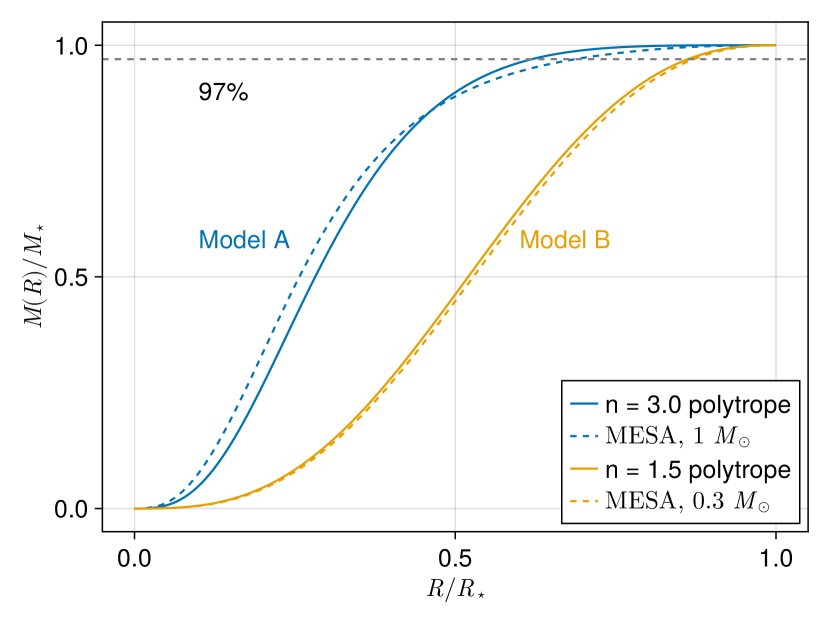
The mass lost in the process of a partial disruption depends on the orbital parameters (in particular on the pericentre distance), and on the internal structure of the star. We will consider two reference cases:
-
•
Model A: a star with mass and radius , , pc.
-
•
Model B: a star with mass and radius , , pc.
where we report the index of the polytropic model that better agrees with the equilibrium MESA profile (Paxton et al., 2010) for the two cases.
In the case of model A, we estimate the mass loss as a function of the pericentre through the fitting formulae obtained by Ryu et al. (2020a, b, c) for stars on nearly radial orbits ()
| (5) |
where is a form factor of order unity that determines the pericentre corresponding to (i.e. a total disruption). When considering a model A star:
| (6) |
In the case we are considering, and , so that .
In the case of model B, we rely on the simulations by Guillochon & Ramirez-Ruiz (2013), that simulated stars with polytropic index . Here the mass loss is given by222The expression of matches the accurate version presented in the erratum (eq. A9).
| (7) |
for . We extrapolate this function at larger pericentre values (i.e. smaller s) as
| (8) |
that is a smooth extrapolation of the main solution up to the second derivative in the log-log space. Although the simulations of Guillochon & Ramirez-Ruiz (2013) were Newtonian, this is an acceptable approximation for partial disruptions around lower-mass MBHs such as our case. The value of the pericentre where the mass is completely lost gives .
The change in orbital energy due to the ejection of material can be crudely estimated from the asymmetry in the tidal field as (Stone et al., 2013; Metzger et al., 2022, eq. 32)
| (9) |
The aforementioned equation assumes a pericentre close to the tidal disruption radius . A more accurate extension to larger pericentres that agrees with hydrodynamical simulations of a star undergoing a partial disruption around an intermediate MBH is simply obtained by replacing with the pericentre of the orbit (Kremer et al., 2022)
| (10) |
An alternative estimate, obtained not from physical reasoning but rather from fitting rational functions to simulations of a star being destroyed by an MBH has been obtained by Gafton et al. (2015)
| (11) |
The two prescriptions show significant difference when is large, while they are comparable (within a factor of 3) when (in Fig. 3 they can be compared directly).
As we already mentioned, tidal forces may also alter the stellar structure, inducing oscillations of the star by converting part of its orbital kinetic energy into the mechanical energy of stellar normal modes. This process, known as tidal excitation (or the “dynamical tide”), increases the orbital binding energy in competition with the effects of mass loss. The energy of the oscillations can be written as (Press & Teukolsky, 1977)
| (12) |
where is a function that depends on the details of the stellar structure. Assuming that the oscillations are weak, one can treat them in the linear regime, and the function can be expanded, giving
| (13) |
where , are the lowest order terms (quadrupolar and octupolar, respectively) in the linear expansion of the tidal field (Lee & Ostriker, 1986). Although these functions involve complicated integrals over the internal structure of the star, we employ the analytic fitting functions of Portegies Zwart & Meinen (1993, eq. 7 and Tab.1, with since ), which are accurate for the polytropic models we use.
When mass loss becomes significant and oscillations are strong, the linear regime becomes inadequate; one must instead solve directly the hydrodynamics of the oscillations. While this is most accurately done with hydrodynamical simulations (Manukian et al., 2013), the tidal coupling driving nonlinear oscillations can be approximated reasonably well with the “extended affine model” of Ivanov & Novikov (2001), a generalization of the classical affine model for tidally disrupting stars (Luminet & Carter, 1986)333The affine model approximates the interior of a star subject to strong tidal perturbations as a set of concentric (but not necessarily co-aligned; Ivanov & Novikov, 2001) ellipsoidal shells with time-evolving axis ratios. In this sense, it can be understood as a nonlinear theory of the quadrupolar tide, neglecting higher-order terms.. In the case of some polytrope models, analytic fits of the extended affine model’s predictions for nonlinear have been presented in Generozov et al. (2018, eq. B1 and B2, ). Since stars described by model A are more centrally concentrated with respect to stars of model B – see Fig. 1 – tidal excitation is generally stronger, compared to asymmetric mass loss effects, in Model B ().
The energy changes presented here allow us to infer whether a star can undergo multiple partial disruptions, and whether it becomes more or less bound at each passage.
2.2 Two-body relaxation and loss cone theory
The dynamical evolution and relaxation of a nuclear cluster due to two-body encounters is simply and accurately described by the orbit-averaged Fokker-Planck equation (Cohn & Kulsrud, 1978). By directly computing the expected stochastic variations of a test star’s orbital parameters, it can be shown that relaxation in squared angular momentum (normalized to the value at the circular orbit of energy ) is more efficient than relaxation in for eccentric orbits. One can identify two time scales (Merritt, 2013):
-
•
is the typical relaxation time for the energy of a particle with semi major axis , where and are the velocity dispersion and the density of the stellar distribution at a distance from the centre, respectively.
-
•
is the typical relaxation time for the angular momentum of the particle.
Since , nearly radial orbits (where stars about to be destroyed are typically located) relax much faster in angular momentum, effectively decoupling the relaxation processes in and for small . This fact has been exploited by Cohn & Kulsrud (1978) to derive a suitable boundary layer solution for the orbit-averaged Fokker-Planck equation in and to consistently include loss cone effects in the equation. Moreover, they derived the expected relaxed distribution of among all the particles with energy , including those that will end up in a tidal disruption. We will briefly describe this derivation, in order to highlight the underlying assumptions.
Since is small compared to the scale radius of the stellar distribution, the value of (the dimensionless angular momentum corresponding to ) is very small for most of the stars in the distribution. Therefore, one typically assumes that the energy is constant and can be treated as a parameter. The orbit-averaged Fokker-Planck equation for the phase space distribution function reduces to
| (14) |
where is the orbit averaged diffusion coefficient, that for very eccentric orbits characterises the effects of 2-body encounters (Merritt, 2013)
| (15) |
Here is the orbital period (we neglect its weak dependence on coming from the stellar potential), while and are the orbit-averaged expectation values of perturbations in and , which depend negligibly on the properties of the star being scattered.444The advective terms are proportional to the mass of the body being scattered, but they are increasingly negligible as goes to zero. It is useful to quantify the strength of angular momentum diffusion by defining:
| (16) |
The quantity is also known as the loss cone occupation fraction or loss cone diffusivity, since the local strength of stochastic kicks determines how many particles on an orbit penetrating will actually reach the pericentre without being scattered back onto a safe orbit. Consequently, inside the loss cone, no particles with are statistically expected when (since relaxation needs more than one orbit to change significantly the pericentre), while many particles are expected at any time when (as their pericentre is likely to change along the orbit due to 2-body encounters). The former is usually referred to as the empty loss cone regime, the latter as the full loss cone regime. The number of orbits required for relaxation to affect the orbital parameters will be a crucial point for our analysis of repeated partial disruptions, since they can happen only if the orbital parameters are negligibly altered by relaxation. Because of the dependency on , the value of in the two models is related as
| (17) |
A common assumption in literature is to employ a reduced equation to evolve a distribution function that does not depend explicitly on , and assumes the steady state distribution of angular momentum at each energy
| (18) |
to compute the rate of tidal disruptions at each energy. The relation between and is directly determined by the model of instantaneous tidal disruptions at the pericentre. The rates are computed from the solution of the 1D evolution in energy (Vasiliev, 2017; Stone et al., 2020)
| (19) |
as
| (20) |
where the pre-factor converts the distribution function into the differential distribution such that the number of stars is given by . As we shall see, the model of a TDE as an instantaneous event is directly related to the estimate of TDE event rates through the computation of .
We summarize here the key assumptions made to derive the relaxed profile in Cohn & Kulsrud (1978):
-
CK 1
A full, terminal disruption occurs at the pericentre if and only if .
-
CK 2
The energy fluctuation timescale is much longer than the angular momentum relaxation timescale.

We will now consider a prototypical system to compute the strength of 2-body relaxation. The system is composed of a central MBH with mass surrounded by a distribution of stars (total number , individual mass ) and stellar black holes (total number , individual mass ) both following a Dehnen profile (Dehnen, 1993; Tremaine et al., 1994) with scale radius of and inner slope , as in Broggi et al. (2022). This system has an influence radius555There are multiple definitions of influence radius in literature. In this work we define , where is the local velocity dispersion. of and the velocity dispersion at the influence radius corresponds to , computed according to the by Gültekin et al. (2009). This system is used to compute the quantity . The loss cone diffusivity in this system is shown in Fig. 2.
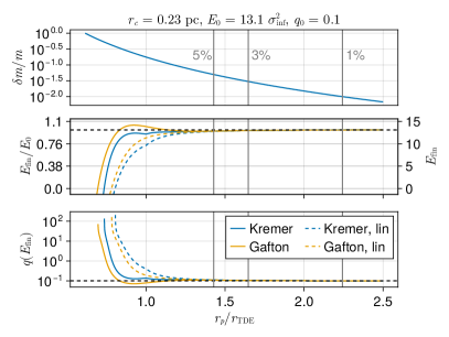
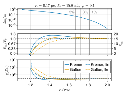
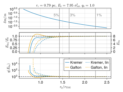
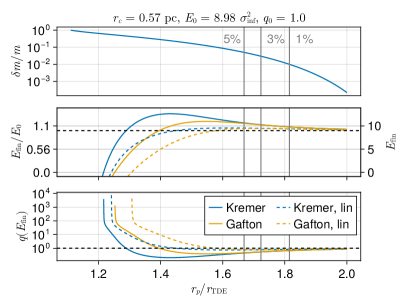
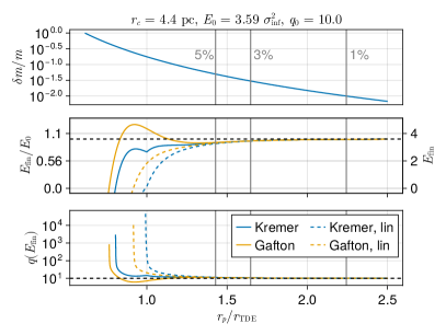
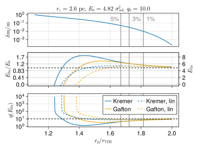
In Fig. 3 we show the predictions of our semi-analytical model for partial disruptions of a star. We consider both model A and model B stars; different values of the initial energy corresponding to ; different prescriptions for energy change in the core kick (Eqs. 10 and 11); and different models for tidal excitation (linear and non-linear).
Irrespective of the specific models used for the computation of energy changes (i.e. tidal excitation and mass loss), there is a qualitative difference between the partial disruption of stars in the two stellar models – such a difference is driven by the different internal structure. The more compact structure of model requires deeper penetration of the orbit (smaller ) for the star to lose mass, so that the function goes to zero at large pericentres faster than to stars described by model A. Moreover, the compact structure of model B corresponds to a larger energy stored into oscillations, with tidal oscillations being dominant at large . On the other hand, partial disruptions of model stars are dominated by the effects of mass loss at larger pericentres. In general, the linear expansion seems to perform well compared to non-linear estimates when mass loss is below approximately . While in the case of model A Eq. 11 predicts a larger energy increase with respect to Eq. 10, the opposite is true in the case of model B given the larger pericentres involved in units of .
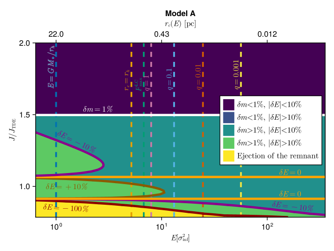
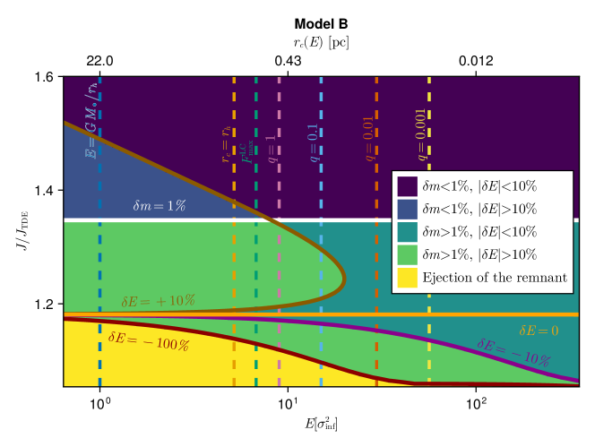
To overview the full energy range, in Fig. 4 we show the qualitative effect of single passages at the pericentre as a function of the initial energy and angular momentum for model A and model B; we also report the radius of a circular orbit at energy for better interpretation. Here, we use the combination of energy change given by Eq. 11 and non-linear tidal excitations of Eq. 12. We plot the contours that correspond to , and , and define some (arbitrary) thresholds to classify the possible outcomes:
-
•
Negligible change in the orbit, negligible change in the mass. We define this to happen when and (dark blue).
-
•
Significant change in the orbit, negligible change in the mass. This happens when and (blue). This only happens in model B.
-
•
Negligible change in the orbit, significant change in the mass. This happens when and (aqua green).
-
•
Significant change in the orbit, significant change in the mass. This happens when and (green).
-
•
Ejection of the remnant. This happens when (yellow).
As with the previous analysis, we see that the two stellar models show different qualitative behaviours for large pericentres. In particular, we see that model A stars have smaller energy fluctuations at , while the tidal excitation is strongly relevant in model B for semimajor axis (estimated through ) comparable to the influence radius. On the other hand, mass loss effects are dominant for model A and the total energy change is positive (i.e, the resulting orbit is more bound) only at small pericentre passages. Close to , the energy fluctuation steeply decreases and the remnant is ejected in both cases.
3 Repeated disruptions and 2-body relaxation
We will now try to assess the impact of single and repeated disruptions, first considering the full loss cone regime, where repeated disruptions are unlikely to occur, and then the empty loss cone regime where repeated partial disruptions are likely to take place. The key variable we will introduce is the number of orbits needed by relaxation to significantly alter the pericentre
| (21) |
so that a repeated partial disruption is likely to occur when .
3.1 Full loss cone regime
When , relaxation acts on timescales shorter than times between two partial disruption events. In this regime, single passages grazing or entering the loss cone radius will alter the orbital parameters once per period , while the timescale of relaxation in angular momentum is . This implies that only a small fraction of stars with pericentre smaller than the tidal disruption radius will actually reach the turning point, but they are likely to be scattered to a different (safe) orbit before. As a consequence, the probability of having a pTDE and staying on the same orbit to undergo a second disruption is small, and virtually negligible since grows quickly as the orbital energy decreases (see Fig. 2).
A fraction of partial disruptions of loosely bound stars may result in the ejection of the remnant at a pericentre larger than (see Fig. 4), and this may be compatible with classical loss cone theory.
In fact, since they both imply an instantaneous removal of the subject star from the distribution, ejections can be treated together with total disruptions in the standard approach to the loss cone, where particles are removed when they reach a pericentre below the critical value . Therefore, by identifying a suitable, larger threshold radius that roughly distinguishes the region of ejections plus total disruptions, classical loss cone theory may be simply adapted to provide a good description of the system. Such a value of weakly depends on energy, but this does not affect the estimation of the corresponding Cohn-Kulsrud solution.
3.2 Empty loss cone regime
In the empty loss cone regime , and repeated partial disruptions are expected. In fact, the empty loss cone regime is defined as the region of phase space where relaxation needs many orbits to alter significantly the orbital parameters of an orbit with the critical pericentre .
Model A Model B
Since we are interested in understanding whether the classical loss cone theory applies to partial disruptions, we need to assess the cumulative effect of repeated partial disruption on the orbits over the local relaxation timescale, that operates in orbits; furthermore, this approach allows us to estimate how many passages a star initially on a partial disruption orbit manages to complete before either being ejected, surviving the interaction without escaping the system, or being fully disrupted.
For each pericentre passage, we will consider the mass lost according to Eq. (5) (model A) or Eq. (7) (model B) and the two prescriptions for the corresponding decrease in specific binding energy via core kicks, also including the exchange of energy between stellar oscillations and orbital motion according to Eq. (12). We remark that the perturbation due to tidal excitation is positive-definite (i.e. the orbit becomes more bound) only at the first pericentre passage. At subsequent passages, whether the tidal deformation injects or subtracts energy to the stellar orbit depends on the phase of the ongoing oscillation (induced by the previous passage) when the star is gets back to pericentre (Lai, 1997). To include this effect, we use Eq. 12 to determine the amplitude of the energy exchanged but, from the second pericentre passage onwards, we give it a random sign at each passage.
For and each stellar model we set up three simulations with the following simple scheme.
-
1.
We set the initial energy corresponding to the chosen value of . We set the initial mass to and the initial angular momentum , where is the angular momentum of the orbit whose pericentre is .
- 2.
-
3.
We use Eq. (10) or Eq. (11) and Eq. (12) to compute the total energy variation
(22) where at the first pericentre passage, and with equal probability at later passages. We keep track of the total energy of the oscillations, and we adjust to damp them completely when their total energy would become negative.
-
4.
We compute the new mass , the new tidal disruption radius , and the new energy .
We repeat steps until
-
•
total disruption ( for model A, for model B),
-
•
ejection (),
-
•
survival (i.e. the star completes orbits).
For each value of we choose 80 equally spaced values in
| (23) |
with and , consistently with step 1 above.
We treat and as fixed parameters throughout the evolution, since modelling the readjustment of the star requires to directly solve the complex hydrodynamic evolution of the stellar structure666Since we are considering orbital periods of at most yr, much less than the Kelvin-Helmholtz timescale ( Myr; Kippenhahn & Weigert, 1990), dramatic mass loss and energy injection through the dissipation of nonlinear oscillation modes can in principle seriously affect the internal structure of the star.. In Appendix A we explore a non-fiducial scenario where the star can inflate due to nonlinear tides. In this case, part of the energy stored in oscillations is converted into internal energy through an enlargement of the radius. Finally, we remark that this procedure implies that the specific angular momentum is constant throughout the repeated disruptions.
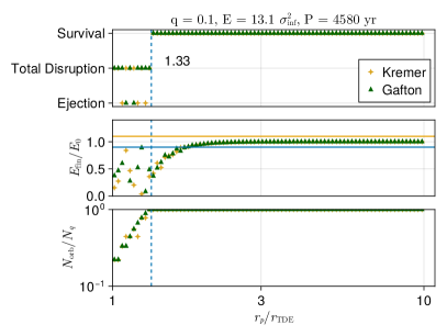
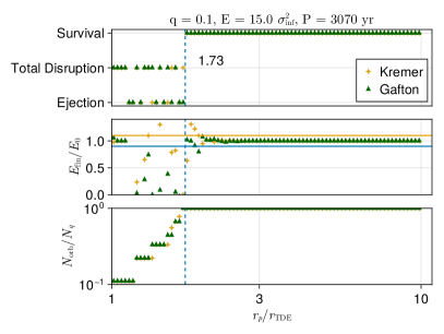
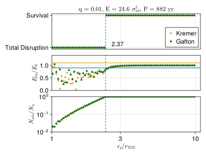
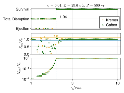
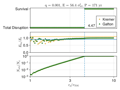
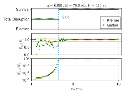
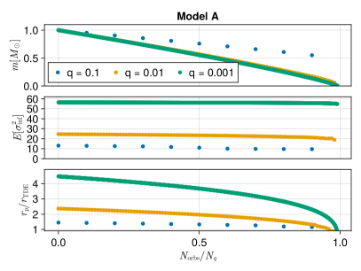
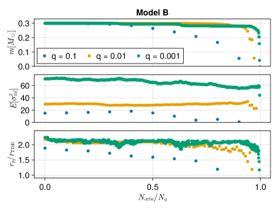
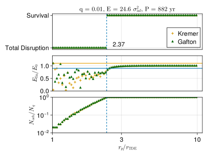
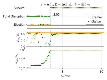
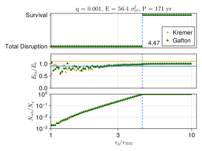
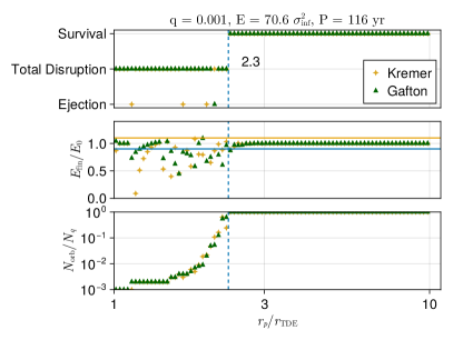
In Fig. 5 we show the results of our simulations by reporting the outcome (survival, total disruption or ejection), the final energy and the number of repeating partial disruption orbits for each simulation as a function of its initial pericentre . For both models and for any value of , we see that repeating the partial disruption process can lead to total disruption and, in a minority of cases, to ejection at pericentres larger than and The threshold radius (reported in units of in each sub-figure) increases with and therefore decreases with . There are, however, some significant differences between the repeated partial disruption of a star described by model A and one described by model B.

In the case of model A, when a star is partially destroyed and manages to survive pericentre passages, it gradually decreases its specific binding energy , ending up on orbits for which is larger: particles slightly above the threshold radius at equal to or will decrease by and respectively. This is consistent with the fact that asymptotically the total energy fluctuation is dominated by the effects of mass loss.
On the other hand, in the case of model B the star may increase its energy up to for the three values of we considered. This is consistent with the fact that asymptotically the total energy fluctuation is dominated by the effects of tidal excitation.
We highlight that, for the cases we considered, each threshold pericentre between total disruption / ejection and survival is consistent between the two models for core kicks, and is such that the linear regime of tidal oscillations is sufficiently accurate (see Fig. 3). Only below the threshold pericentre the non-linear description of tidal oscillations must be taken into account.
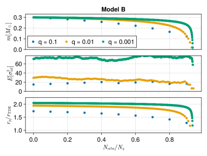
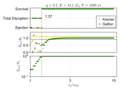
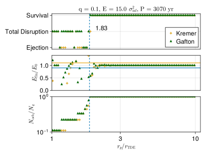
In Fig. 6 we show the trajectories at the threshold pericentre for both models. The plot shows that model A corresponds to a gradual decrease of , while model B corresponds to fluctuations of because of tidal excitation. By construction, the angular momentum of the star is conserved along the evolution, so that the pericentre is constant too: is recomputed at each step with the updated energy, but the fluctuations are at most of one part in for these orbits. Therefore, the key change in the process is the enlargement of due to mass loss, so that within a small number of orbits (compared to ) the mass is fast depleted up to the total disruption (upper panel). The energy of the star, on the other hand, shows an evolution that depends on the stellar model and the particular pericentre, and for and clearly follows the expectation based on the large trend.
4 Discussion and conclusions
We presented a simple semi-analytical model of partial disruptions for two stellar models, one for main sequence stars with mass and the other for main sequence stars with mass . The prescriptions included in our semi-analytical models are based on the results of hydrodynamical simulations and semi-analytic modeling (Ryu et al., 2020a, b, c, d; Guillochon & Ramirez-Ruiz, 2013; Gafton et al., 2015; Kremer et al., 2022; Stone et al., 2013; Ivanov & Novikov, 2001). To properly study the phenomenon in the empty loss cone regime, where relaxation needs more than one orbit to change the orbital parameters, we accounted for the possibility of repeating partial disruptions. We will now discuss the implications of our model for the inclusion of partial disruptions in the loss cone theory, and the computation of their event rate.
4.1 Partial disruptions and loss cone theory
In the theory of the loss cone, one can use a Monte Carlo or a Fokker Planck approach to study the evolution of the distribution function of a stellar system (Cohn & Kulsrud, 1978; Shapiro & Marchant, 1978). These studies show that particles enter the critical radius of the loss cone once are driven there by the stochastic encounters; in particular they typically start with a pericentre larger than the critical value and are then driven on orbits penetrating the critical sphere.
In the full loss cone regime, particles approaching the loss cone boundary can be scattered at any pericentre value (Merritt, 2013), so that all possible outcomes (i.e. partial disruption with orbital and mass change, ejection or total disruption) can occur. Neglecting the change in energy and mass, one can apply the classical loss cone theory - based on the instantaneous disruption model - to account for ejections and therefore use the corresponding (larger) critical pericentre.
In the empty loss cone regime, the stellar model plays an important role. For stars of (i.e. star model A), our model predicts that for (and larger values up to ) stars approaching the loss cone in phase space by gradually reducing their pericentre due to 2-body interactions will likely reduce their specific binding energy significantly (more than ). Consequently, stars will move to a region where is larger - where they can be scattered away from the loss cone, or being disrupted / ejected at an energy different from the initial one. Only at very small , as in the case of , the energy change is so small that the particle will likely proceed towards total disruption through a sequence of very small partial disruption events. The classical picture based on instantaneous disruption cannot be therefore adapted, as we proposed for the full loss cone regime. Here, the phenomenon of partial disruptions will effectively alter the energy of the particles approaching the loss cone, invalidating the assumption CK2, i.e. the fact that the (stochastic) relaxation of can determine the expected relaxed profile in phase space.
Stars described by model B, on the other hand, show a difference: the specific binding energy is subject to significant fluctuations, as these compact stars are more susceptible to tidal excitation. The orbital energy can change by more than as the star approaches the loss cone boundary, with a bias towards tighter configurations when considering Kremer’s estimate for mass loss (Eq. 10). This means that the star may be moved to regions where is smaller and two-body interactions less efficient. This process is somehow similar to that of extreme mass ratio inspirals (EMRIs), a phenomenon where a compact object approaches the central MBH so close that its evolution is deterministically driven by GWs emission over hundreds of thousand of orbits (Amaro-Seoane, 2018). In this case, the role of the emission of GWs at each pericentre passage would be replaced by a small mass loss and consequent tidal excitation. The total event rate of EMRIs (but not the distribution at capture) is computed by integrating the classically expected rate – with the loss cone radius equal to the innermost parabolic orbit – over the region where one expects EMRIs to be formed (Hopman & Alexander, 2005; Bar-Or & Alexander, 2016). For stars of model B, a tentative approach to compute the total number of stars undergoing a partial disruption may be therefore to integrate the classical rate over the phase-space region where . However, the information about the number of repeated partial disruptions that each of these stars undergoes must be inserted with a more detailed model.
As we mentioned at the beginning of this section, relaxation in the empty loss cone regime mainly drives particles from larger to smaller angular momenta/pericentres. This means that stars will gradually approach the critical thresholds identified in Fig. 5 from right to left in the plots, effectively resulting in a sequence of weak partial disruptions as shown in Fig. 6. As decreases, the mass lost at each pericentre passage is smaller, and therefore the resulting electromagnetic flare is expected to be weaker (Stone et al., 2020; Rossi et al., 2021).
4.2 Implications for TDE rates
Currently available estimates of time-evolving TDE rates rely on the assumption that the relaxed profile in angular momentum of stars is described by the CK solution, either in the whole range of , as in 1D Fokker Planck approaches (e.g. Vasiliev, 2017; Stone & Metzger, 2016) or as the boundary condition at the loss cone interface for 2D models (e.g. Broggi et al., 2022). It is of primary interest to understand how these results should be interpreted when relaxing the hypothesis of instantaneous disruption.
The efficiency of two-body relaxation in altering the orbital parameters when implies that the classically computed rates are reliable in this regime, and should be computed with a loss cone radius slightly larger than accounting for the possibility of ejections due to mass loss ( and for the models we considered). Among the events computed this way, one should identify the pericentres resulting into observable events, as discussed in Bortolas et al. (2023).
The case of partial disruptions in the empty loss cone regime instead requires a more careful treatment. As a first order effect, when , particles at pericentres up to for model A and for model B will be affected by the presence of the loss cone. At smaller value of , therefore higher specific binding energy, we expect this pericentre to increase due to the higher number of orbits allowed. This will correspond to a larger rate of partial disruptions, possibly repeating. Moreover, both models predict a significant change of the specific binding energy for particles as they approach the identified total disruption zone, with higher values of corresponding to stronger alterations. In the case of model A stars, part of the classically predicted rate will therefore result in failed disruptions, since particles will be moved to higher areas as the sequence of weak partial disruptions takes place. On the other hand, model B stars might increase their specific binding energy completing the sequence of weak disruptions. In both cases, the inclusion of partial disruptions in Fokker-Planck solvers requires a proper modeling of the phenomenon accounting for modifications to the Cohn-Kulsrud profile, see Eq. 18.
For all models, the inclusion of repeated partial disruptions implies that a fraction of the classically expected TDEs will actually correspond to a sequence of weak disruptions, that may be too weak to be detected (Rossi et al., 2021; Stone et al., 2020), but can still contribute to the growth of the MBH. The large number of consecutive desruptions with weak mass loss may result in a sequence of bursts of gravitational waves, possibly increasing the gravitational wave background from TDEs (Toscani et al., 2020).
It has been estimated that most of the TDEs originates in the empty loss cone regime, with a fraction approximately given by (Stone & Metzger, 2016, eq. 29)
| (24) |
corresponding to of the total expected cosmological rate. A qualitative result of our analysis is that part of these classically expected events will correspond to non-detectable pTDEs, therefore possibly reconciling the observed discrepancy between observed and expected TDE rates (Stone et al., 2020; van Velzen, 2018), while mantaining the possibility that stellar captures contribute to the growth of MBHs.
4.3 Caveats
In the case of model A, we determined the mass lost at the pericentre passage through Eq. 5. This equation has been derived for a MESA star with the core hydrogen mass fraction of 0.5 (Ryu et al., 2020a) on a parabolic orbit. On the other hand, the effect of tidal excitation has been included through a prescription valid for polytropes. The MESA profile and the polytropic model correspond to different tidal excitation, with MESA model subject to stronger oscillations as shown in Generozov et al. (2018) (the corresponding function is larger by a factor of a few).
On the other hand, when considering model B, we used the estimate for from the simulations by Guillochon & Ramirez-Ruiz (2013). These do not account for relativistic effects, that are increasingly important as the mass of the central MBH grows and the pericentre of the orbit of partial disruption decreases.
Liu et al. (2024) simulated the partial disruption of different stars on orbits with eccentricity around an MBH with mass . The simulations include the disruption of a star with radius initially described by a MESA model (corresponding to our model A stars). At small penetration factors, corresponding to weak mass loss, the simulated stars get slightly more tightly bound to the central MBH, the opposite of our predictions, showing a trend similar to what we expect for the less concentrated model B stars. In addition to the inconsistency between the MESA profile and the polytrope, this qualitative difference may also arise from the specific orbital parameters. In fact Eq.5 (the function relating the pericentre distance and the mass lost at the pericentre passage 5) has been fit to the simulation of disruptions on orbits (Ryu et al., 2020a, b, c), and the tidal excitation prescription similarly assume a parabolic orbit (Lee & Ostriker, 1986; Ivanov & Novikov, 2001). In general, the time spent at the pericentre increases as the eccentricity decreases, affecting both asymmetric mass loss and tidal excitation.
A general assumption in our treatment of repeating partial disruptions is that the stellar profile evolves self-similarly - with the same radius and the same polytropic index . However, it is natural to expect that strong non-linear excitation and significant mass loss will result in a readjustment of the stellar profile and change, for example, the best fitting polytropic index. In general, when mass loss is extremely weak the outer layers of the star may expand to locally compensate the stripping. Moreover, as tidal oscillations become stronger, it is possible that part of the energy they store may thermalise and trigger a readjustment of the stellar profile, possibly by enlarging the radius of the star. In Appendix A we explore this possibility and show that this effect mainly affects stars described by model B. In fact, being dominated by tidal excitation effects at larger , model B stars can end up in a total disruption at slightly larger pericentre compared to the reference scenario. Overall, the qualitative picture we discussed seems generally insensitive to stellar expansion, but we caution that our model for this is approximate and the matter should be investigated further with hydrodynamical simulations.
The model we built for partial disruptions holds only on a range of MBH masses. Repeated disruptions at small penetration factors may completely disrupt a star as long as the motion of the central MBHs around the centre of the system is negligible with respect to the orbital timescales, setting a lower bound to the mass of the central MBH. On the other hand, the star can undergo a disruption as long as it is not gravitationally captured before the disruption, setting an upper bound to the mass of the central black hole ( for a sun-like star, the Hills mass). Finally, when the mass of the central black hole is large, one should account for general relativistic effects affecting the disruption process (Coughlin & Nixon, 2022) and the tidal excitation of the surviving core (Ivanov et al., 2003).
Finally, we included relaxation in our model only by setting the maximum number of pericentre passages that a repeating pTDE can perform. However, a more complete treatment should include discrete orbital fluctuations (in energy and angular momentum), e.g. in a Monte Carlo fashion (Shapiro & Marchant, 1978). This will result, for example, in the possibility of interrupting the sequence of weak partial disruptions with a stronger event even in the empty loss cone regime (Weissbein & Sari, 2017).
4.4 Summary and Conclusions
We have constructed a simple model for the partial disruption of a star around a massive black hole. We estimated of the number of consecutive partial disruptions that a star will undergo depending on the strength of two-body encounters, and estimated the final outcome of the sequence of disruptions as a function of the initial pericentre distance. We considered two stellar models of and , taking these two values as roughly representative of lower-main sequence and upper-main sequence internal structures. We then built a model for partial disruptions that accounts for the effects of mass loss and tidal excitation of the stellar structure. We built our model based on the results of hydrodynamical simulations (Ryu et al., 2020a, b, c, d; Guillochon & Ramirez-Ruiz, 2013; Gafton et al., 2015) and previous theoretical studies (Kremer et al., 2022; Stone et al., 2013; Ivanov & Novikov, 2001). For each model we studied the problem of single partial disruptions, arguing that this is the relevant problem for loss cone orbits ( comparable to ) with binding energy small enough that two-body relaxation is efficient, i.e. in the full loss cone regime. We then considered the phenomenon of repeated partial disruptions, estimating the number of passages as the inverse of the loss cone occupation fraction , as in Eq. (21). Therefore, pTDEs are expected to occur in the empty loss cone regime.
The main results of our work are summarised below:
-
•
The phenomenon of ejections, that is caused by significant mass loss in partial disruptions, may effectively enlarge the loss cone radius by 20% compared to .
-
•
Partial disruptions may alter the orbital energy without destroying the stars. For stars with , weak pTDEs happening at pericentres larger than will result in a less tightly bound remnant. For stars with , weak pTDEs happening at pericentres larger than will result in a more tightly bound remnan.
-
•
Stars in the empty loss cone are kicked by two-body relaxation towards orbits with smaller pericentres. Regardless of the stellar model, they are likely being consumed by a sequence of weak pTDEs. Only for stars we find the possibility of being scattered onto a total TDE or away from the loss cone because of significant energy fluctuations when is small ().
-
•
TDEs originating in the empty loss cone may correspond to unobservable events. Since 70 % of the TDEs are expected to originate in the empty loss cone regime, accounting for repeating pTDEs may reconcile expectations and observations of the total observed TDE rate.
We conclude by noting that our results strongly depend on the interplay of mass loss effects and tidal excitation. The simulation of a star being repeatedly disrupted by a MBH is currently too computationally expensive, since one needs to describe the hydrodynamical structure of the star including self gravity. The large computational cost is primarily due to the need of following a star along its nearly-radial orbit. However, a better understanding of repeating pTDEs offers a promising tentative solution for the tension between observational TDE rates and theoretical estimates.
Acknowledgements
LB thanks Alessandro Lupi and Martina Toscani for useful discussions.
MB acknowledges support provided by MUR under grant “PNRR - Missione 4 Istruzione e Ricerca - Componente 2 Dalla Ricerca all’Impresa - Investimento 1.2 Finanziamento di progetti presentati da giovani ricercatori ID:SOE_0163” and by University of Milano-Bicocca under grant “2022-NAZ-0482/B”.
LB, EB and AS acknowledge the financial support provided under the European
Union’s H2020 ERC Consolidator Grant “Binary Massive Black Hole Astrophysics” (B Massive, Grant Agreement: 818691).
EB acknowledges support from the European Union’s Horizon Europe programme under the Marie Skłodowska-Curie grant agreement No 101105915 (TESIFA), from the European
Consortium for Astroparticle Theory in the form of an Exchange Travel Grant, and the European Union’s Horizon 2020 Programme under the AHEAD2020 project
(grant agreement 871158). NCS was supported by the Israel Science Foundation (Individual Research Grant 2565/19) and the Binational Science Foundation (grant Nos. 2019772 and 2020397).
Software: the Julia language (Bezanson et al., 2017); Makie.jl (Danisch & Krumbiegel, 2021); Roots.jl (Verzani, 2020); Interpolations.jl (Kittisopikul &
Holy, 2023).
Appendix A Expansion due to tidal oscillations
We report here a set of simulations that allow for the conversion of energy stored in oscillations into internal energy of the star. This is implemented through an expansion of the star, computed between step 3 and step 4 of the procedure outlined in 3.2. This is expected to happen only when the oscillations of the stellar structure are strongly non-linear. To estimate when this happens, we compare the total energy stored in oscillations with the internal energy of the star. For a polytrope model with index (Chandrasekhar, 1957)
| (25) |
When (an arbitrary threshold) we enlarge the stellar radius by a quantity
| (26) |
and update consistently
| (27) |
In Fig. 7 and 8 we report the orbits at the threshold value of and the overview of the outcomes at , and .
Compared to the reference model presented in the text, partial disruptions will completely destroy stars up to larger pericentre values. The effect is evident for model B stars, since they are strongly affected by tidal excitation at larger . Qualitatively, the results of this simulations are consistent with the conclusions presented in the main text.
References
- Amaro-Seoane (2018) Amaro-Seoane, P. 2018, Living Reviews in Relativity, 21, 4
- Bar-Or & Alexander (2016) Bar-Or, B. & Alexander, T. 2016, The Astrophysical Journal, 820, 129
- Bezanson et al. (2017) Bezanson, J., Edelman, A., Karpinski, S., & Shah, V. B. 2017, SIAM Review, 59, 65
- Bloom et al. (2011) Bloom, J. S., Giannios, D., Metzger, B. D., et al. 2011, Science, 333, 203
- Bortolas et al. (2023) Bortolas, E., Ryu, T., Broggi, L., & Sesana, A. 2023, Partial Stellar Tidal Disruption Events and Their Rates
- Broggi et al. (2022) Broggi, L., Bortolas, E., Bonetti, M., Sesana, A., & Dotti, M. 2022, Monthly Notices of the Royal Astronomical Society, 514, 3270
- Cenko et al. (2012) Cenko, S. B., Krimm, H. A., Horesh, A., et al. 2012, The Astrophysical Journal, 753, 77
- Chandrasekhar (1942) Chandrasekhar, S. 1942, Principles of Stellar Dynamics
- Chandrasekhar (1957) Chandrasekhar, S. 1957, An Introduction to the Study of Stellar Structure.
- Chen & Shen (2021) Chen, J.-H. & Shen, R.-F. 2021, ApJ, 914, 69
- Cohn & Kulsrud (1978) Cohn, H. & Kulsrud, R. M. 1978, The Astrophysical Journal, 226, 1087
- Coughlin & Nixon (2019) Coughlin, E. R. & Nixon, C. J. 2019, ApJ, 883, L17
- Coughlin & Nixon (2022) Coughlin, E. R. & Nixon, C. J. 2022, The Astrophysical Journal, 936, 70
- Danisch & Krumbiegel (2021) Danisch, S. & Krumbiegel, J. 2021, Journal of Open Source Software, 6, 3349
- Dehnen (1993) Dehnen, W. 1993, Monthly Notices of the Royal Astronomical Society, 265, 250
- Evans & Kochanek (1989) Evans, C. R. & Kochanek, C. S. 1989, ApJ, 346, L13
- Frank & Rees (1976) Frank, J. & Rees, M. J. 1976, Monthly Notices of the Royal Astronomical Society, 176, 633
- French et al. (2016) French, K. D., Arcavi, I., & Zabludoff, A. 2016, The Astrophysical Journal, 818, L21
- French et al. (2020) French, K. D., Wevers, T., Law-Smith, J., Graur, O., & Zabludoff, A. I. 2020, Space Sci. Rev., 216, 32
- Gafton et al. (2015) Gafton, E., Tejeda, E., Guillochon, J., Korobkin, O., & Rosswog, S. 2015, Monthly Notices of the Royal Astronomical Society, 449, 771
- Generozov et al. (2018) Generozov, A., Stone, N. C., Metzger, B. D., & Ostriker, J. P. 2018, Monthly Notices of the Royal Astronomical Society, 478, 4030
- Gezari (2021) Gezari, S. 2021, Annual Review of Astronomy and Astrophysics, 59, 21
- Guillochon & Ramirez-Ruiz (2013) Guillochon, J. & Ramirez-Ruiz, E. 2013, ApJ, 767, 25
- Guillochon & Ramirez-Ruiz (2013) Guillochon, J. & Ramirez-Ruiz, E. 2013, The Astrophysical Journal, 767, 25
- Gültekin et al. (2009) Gültekin, K., Richstone, D. O., Gebhardt, K., et al. 2009, The Astrophysical Journal, 698, 198
- Hills (1975) Hills, J. G. 1975, Nature, 254, 295
- Hils & Bender (1995) Hils, D. & Bender, P. L. 1995, The Astrophysical Journal, 445, L7
- Hopman & Alexander (2005) Hopman, C. & Alexander, T. 2005, The Astrophysical Journal, 629, 362
- Ivanov et al. (2003) Ivanov, P. B., Chernyakova, M. A., & Novikov, I. D. 2003, Monthly Notices of the Royal Astronomical Society, 338, 147
- Ivanov & Novikov (2001) Ivanov, P. B. & Novikov, I. D. 2001, The Astrophysical Journal, 549, 467
- Kippenhahn & Weigert (1990) Kippenhahn, R. & Weigert, A. 1990, Stellar Structure and Evolution
- Kittisopikul & Holy (2023) Kittisopikul, M. & Holy, T. E. 2023, JuliaMath/Interpolations.Jl
- Kremer et al. (2022) Kremer, K., Lombardi, J. C., Lu, W., Piro, A. L., & Rasio, F. A. 2022, The Astrophysical Journal, 933, 203
- Krolik et al. (2020) Krolik, J., Piran, T., & Ryu, T. 2020, ApJ, 904, 68
- Lai (1997) Lai, D. 1997, The Astrophysical Journal, 490, 847
- Lee & Ostriker (1986) Lee, H. M. & Ostriker, J. P. 1986, The Astrophysical Journal, 310, 176
- Leloudas et al. (2016) Leloudas, G., Fraser, M., Stone, N. C., et al. 2016, Nature Astronomy, 1, 0002
- Lightman & Shapiro (1977) Lightman, A. P. & Shapiro, S. L. 1977, The Astrophysical Journal, 211, 244
- Lin et al. (2022) Lin, Z., Jiang, N., Kong, X., et al. 2022, ApJ, 939, L33
- Liu et al. (2023a) Liu, C., Mockler, B., Ramirez-Ruiz, E., et al. 2023a, ApJ, 944, 184
- Liu et al. (2023b) Liu, Z., Malyali, A., Krumpe, M., et al. 2023b, A&A, 669, A75
- Liu et al. (2024) Liu, Z., Ryu, T., Goodwin, A. J., et al. 2024, Rapid Evolution of the Recurrence Time in the Repeating Partial Tidal Disruption Event eRASSt J045650.3-203750
- Lodato et al. (2009) Lodato, G., King, A. R., & Pringle, J. E. 2009, MNRAS, 392, 332
- Luminet & Carter (1986) Luminet, J. P. & Carter, B. 1986, The Astrophysical Journal Supplement Series, 61, 219
- Magorrian et al. (1998) Magorrian, J., Tremaine, S., Richstone, D., et al. 1998, AJ, 115, 2285
- Mainetti et al. (2017) Mainetti, D., Lupi, A., Campana, S., et al. 2017, A&A, 600, A124
- Malyali et al. (2023a) Malyali, A., Liu, Z., Merloni, A., et al. 2023a, MNRAS [\eprint[arXiv]2301.05484]
- Malyali et al. (2023b) Malyali, A., Liu, Z., Rau, A., et al. 2023b, MNRAS [\eprint[arXiv]2301.05501]
- Manukian et al. (2013) Manukian, H., Guillochon, J., Ramirez-Ruiz, E., & O’Leary, R. M. 2013, The Astrophysical Journal, 771, L28
- Merritt (2013) Merritt, D. 2013, Dynamics and Evolution of Galactic Nuclei (Princeton University Press)
- Metzger et al. (2022) Metzger, B. D., Stone, N. C., & Gilbaum, S. 2022, The Astrophysical Journal, 926, 101
- Miles et al. (2020) Miles, P. R., Coughlin, E. R., & Nixon, C. J. 2020, ApJ, 899, 36
- Paxton et al. (2010) Paxton, B., Bildsten, L., Dotter, A., et al. 2010, The Astrophysical Journal Supplement Series, 192, 3
- Payne et al. (2021) Payne, A. V., Shappee, B. J., Hinkle, J. T., et al. 2021, ApJ, 910, 125
- Phinney (1989) Phinney, E. S. 1989, in IAU Symposium, Vol. 136, The Center of the Galaxy, ed. M. Morris, 543
- Polkas et al. (2023) Polkas, M., Bonoli, S., Bortolas, E., et al. 2023, arXiv e-prints, arXiv:2312.13242
- Portegies Zwart & Meinen (1993) Portegies Zwart, S. F. & Meinen, A. T. 1993, Astronomy and Astrophysics, 280, 174
- Press & Teukolsky (1977) Press, W. H. & Teukolsky, S. A. 1977, The Astrophysical Journal, 213, 183
- Rees (1988) Rees, M. J. 1988, Nature, 333, 523
- Rossi et al. (2021) Rossi, E. M., Stone, N. C., Law-Smith, J. A. P., et al. 2021, Space Science Reviews, 217, 40
- Roth et al. (2021) Roth, N., van Velzen, S., Cenko, S. B., & Mushotzky, R. F. 2021, ApJ, 910, 93
- Ryu et al. (2020a) Ryu, T., Krolik, J., Piran, T., & Noble, S. C. 2020a, ApJ, 904, 98
- Ryu et al. (2020b) Ryu, T., Krolik, J., Piran, T., & Noble, S. C. 2020b, ApJ, 904, 99
- Ryu et al. (2020c) Ryu, T., Krolik, J., Piran, T., & Noble, S. C. 2020c, ApJ, 904, 100
- Ryu et al. (2020d) Ryu, T., Krolik, J., Piran, T., & Noble, S. C. 2020d, ApJ, 904, 101
- Sazonov et al. (2021) Sazonov, S., Gilfanov, M., Medvedev, P., et al. 2021, arXiv e-prints, arXiv:2108.02449
- Shapiro & Marchant (1978) Shapiro, S. L. & Marchant, A. B. 1978, The Astrophysical Journal, 225, 603
- Somalwar et al. (2023) Somalwar, J. J., Ravi, V., Yao, Y., et al. 2023, The first systematically identified repeating partial tidal disruption event
- Stone et al. (2013) Stone, N., Sari, R., & Loeb, A. 2013, Monthly Notices of the Royal Astronomical Society, 435, 1809
- Stone & Metzger (2016) Stone, N. C. & Metzger, B. D. 2016, Monthly Notices of the Royal Astronomical Society, 455, 859
- Stone et al. (2020) Stone, N. C., Vasiliev, E., Kesden, M., et al. 2020, Space Sci. Rev., 216, 35
- Stone et al. (2020) Stone, N. C., Vasiliev, E., Kesden, M., et al. 2020, Space Science Reviews, 216, 35
- Syer & Ulmer (1999) Syer, D. & Ulmer, A. 1999, MNRAS, 306, 35
- Teboul et al. (2024) Teboul, O., Stone, N. C., & Ostriker, J. P. 2024, MNRAS, 527, 3094
- Toscani et al. (2020) Toscani, M., Rossi, E. M., & Lodato, G. 2020, Monthly Notices of the Royal Astronomical Society, 498, 507
- Tremaine et al. (1994) Tremaine, S., Richstone, D. O., Byun, Y.-I., et al. 1994, The Astronomical Journal, 107, 634
- van Velzen (2018) van Velzen, S. 2018, ApJ, 852, 72
- Vasiliev (2017) Vasiliev, E. 2017, arXiv:1709.04467 [astro-ph] [\eprint[arxiv]1709.04467]
- Verzani (2020) Verzani, J. 2020, Roots.jl: Root finding functions for Julia, https://github.com/JuliaMath/Roots.jl
- Wang & Merritt (2004) Wang, J. & Merritt, D. 2004, ApJ, 600, 149
- Weissbein & Sari (2017) Weissbein, A. & Sari, R. 2017, Monthly Notices of the Royal Astronomical Society, 468, 1760
- Wevers et al. (2023) Wevers, T., Coughlin, E. R., Pasham, D. R., et al. 2023, ApJ, 942, L33
- Wevers & Ryu (2023) Wevers, T. & Ryu, T. 2023, arXiv e-prints, arXiv:2310.16879
- Yao et al. (2023) Yao, Y., Ravi, V., Gezari, S., et al. 2023, arXiv e-prints, arXiv:2303.06523
- Zhong et al. (2022) Zhong, S., Li, S., Berczik, P., & Spurzem, R. 2022, ApJ, 933, 96