The Rosenzweig-Porter model revisited for the three Wigner-Dyson symmetry classes

Abstract

Interest in the Rosenzweig-Porter model, a parameter-dependent random-matrix model that interpolates between Poisson and Wigner-Dyson (WD) statistics, has come up again in recent years in the field of many-body quantum chaos. The reason is that the model exhibits parameter ranges in which the eigenvectors are Anderson-localized, non-ergodic (fractal) and ergodic extended, respectively. The central question is how these phases and their transitions can be distinguished through properties of the eigenvalues and eigenvectors. We present numerical results for all symmetry classes of Dyson’s threefold way. We analyzed the fluctuation properties in the eigenvalue spectra, and compared them with existing and new analytical results. Based on these results we propose characteristics of the short- and long-range correlations as measures to explore the transition from Poisson to WD statistics. Furthermore, we performed in-depth studies of the properties of the eigenvectors in terms of the fractal dimensions, the Kullback-Leibler (KL) divergences and the fidelity susceptibility. The ergodic and Anderson transitions take place at the same parameter values and a finite size scaling analysis of the KL divergences at the transitions yields the same critical exponents for all three WD classes, thus indicating superuniversality of these transitions.

I Introduction

Random matrix theory (RMT) [1] has been successful in the description of the fluctuation properties in the energy spectra of atomic nuclei [2, 3, 4, 5, 6, 7, 8, 9] and, within the field of quantum chaos, of those of quantum systems with a chaotic classical counterpart. The objective of quantum chaos is to identify signatures of classical chaos in the properties of quantum systems. However, nuclear many-body systems do not have an obvious classical analogue, even though their spectra exhibit features that are similar to those of quantum systems with integrable, chaotic or mixed integrable-chaotic dynamics [10]. It was demonstrated in Refs. 11, 12 that integrability may be associated with collective excitations, i.e. collective motion of the nucleons, whereas chaoticity corresponds to complex motion. In fact RMT, was introduced by Wigner to describe the spectral properties of nuclei [2, 3, 5, 7, 13, 14]. In Refs. 15, 16, 17 a link between the spectral properties of quantum systems with a chaotic dynamics and random Hermitian matrices with Gaussian-distributed matrix elements was proposed. This idea was pursued and led to the Bohigas-Giannoni-Schmit (BGS) conjecture [18] which states that the spectral properties of typical quantum systems, that belong to either the orthogonal ($\beta=1$) universality class, which applies to integer spin systems with preserved time-reversal (${\mathcal{T}}\,$) invariance, to the unitary one ($\beta=2$), when ${\mathcal{T}}$-invariance is violated, or to the symplectic one ($\beta=4$) for half-integer spin systems with preserved ${\mathcal{T}}$-invariance, agree with those of random matrices from the corresponding Wigner-Dyson (WD) ensembles. These comprise the Gaussian orthogonal ensemble (GOE), the Gaussian unitary ensemble (GUE), and the Gaussian symplectic ensemble (GSE), respectively [1, 19]. On the other hand, Berry and Tabor demonstrated, based on the Einstein-Brillouin-Keller quantization [20], that the fluctuation properties in the eigenvalue sequences of typical integrable systems ($\beta=0$) exhibit Poissonian statistics. The BGS conjecture was confirmed for single-particle systems theoretically for all three universality classes [21, 22, 23, 19] and also experimentally, e.g., with flat, cylindrical microwave resonators [24, 25, 26, 27] simulating quantum billiards and microwave networks simulating quantum graphs [28, 29, 30]. It also applies to quantum systems with chaotic classical dynamics and partially violated ${\mathcal{T}}$-invariance [31, 32, 33, 34]. These are described by a RMT model interpolating between the GOE and the GUE for complete ${\mathcal{T}}$-invariance violation. Such systems were investigated theoretically in Refs. 35, 36, 8, 37, 36 and experimentally in microwave billiards [38, 39, 40, 41].

We report in this work on the analysis of the properties of a random matrix model, the Rosenzweig-Porter model (RP), which is a paradigmatic model for the description of universal properties of typical quantum systems, whose classical counterpart undergoes a transition from integrable to chaotic dynamics, leading to a transition from Poisson to Wigner-Dyson statistics of their spectral properties and a transition from localized to extended for their eigenvectors. The RP model was introduced in 1960 to describe phenomena like level repulsion or partial level clustering, exhibited by the energy levels that were obtained from experimental atomic spectra [42]. Depending on a parameter $\lambda$ it interpolates between random matrices from either of the WD ensembles and random diagonal matrices, denoted $\hat{H}^{\beta}$ and $\hat{H}_{0}$, respectively,

$$\hat{H}^{0\to\beta}(\lambda)=\hat{H}_{0}+\lambda\hat{H}^{\beta}\,,\,\beta=1,2,4.$$ (1)

Here, we choose Gaussian distributed random entries for $\hat{H}_{0}$. Upon increasing $\lambda$, the relative strength of off-diagonal matrix elements with respect to diagonal ones increases, and the spectral properties experience a transition from Poisson to WD statistics, while the eigenvectors undergo a transition from localized to extended ergodic phase. Recently, the transition from Poisson to GUE was studied experimentally with a microwave billiard [43].

It was shown in Ref. 44 that a suitable re-parametrization of $\lambda$ in terms of a power law of the matrix dimension uncovers an additional, intermediate phase, consisting of extended non-ergodic eigenstates that exhibit fractal dimensions, referred to as generalized Rosenzweig-Porter (gRP) model in the following. Like in the original model (1) the random matrices $\hat{H}^{\rm gRP}(\gamma)$ of the gRP model are Gaussian distributed, however the variances of the off-diagonal elements are modified by multiplication with an $N$-dependent prefactor,

$$H^{\rm gRP}_{nm}(\gamma)=H_{nn}\delta_{nm}+\frac{1}{N^{\gamma/2}}H_{nm}(1-\delta_{nm})$$ (2)

$$\sigma_{d}^{2}=\langle H_{nn}^{2}\rangle=\frac{1}{\beta N},\,\sigma_{off}^{2}=\left\langle\left(H^{(\xi)}_{nm}\right)^{2}\right\rangle=\frac{1}{2\beta N},\,\xi=0,\dots,\beta-1,\,\beta=1,2,4,$$ (3)

where $N,\,\sigma_{d}^{2},\,\sigma_{off}^{2}$ denote the dimension of $\hat{H}$ and the diagonal and off-diagonal variances, respectively. The parameter $\xi$ counts the number of independent components of the off-diagonal matrix elements of $\hat{H}$ and $\gamma$ determines the phase diagram. For $\beta=1$ $\hat{H}^{\rm gRP}(\gamma)$ is real symmetric, for $\beta=2$ it is complex Hermitian and for $\beta=4$ it is quaternion real and can be written in the quaternion representation. Assuming that $\hat{H}^{\beta=4}$ is $2N$-dimensional, it is given in terms of an $N\times N$ matrix whose matrix elements are $2\times 2$ quaternion matrices of the form,

$$\hat{h}_{mn}=h^{(0)}_{mn}\hbox{$1\hskip-1.2pt\vrule depth=0.0pt,height=6.88889pt,width=0.7pt\vrule depth=0.0pt,height=0.3pt,width=1.19995pt$}_{2}+\bm{h}_{mn}\cdot\bm{\tau},\,n,m=1,\dots,N.$$ (4)

Here, $\hbox{$1\hskip-1.2pt\vrule depth=0.0pt,height=6.88889pt,width=0.7pt\vrule depth=0.0pt,height=0.3pt,width=1.19995pt$}_{2}$ is the 2-dimensional unit matrix, and $\bm{\tau}=-i\bm{\sigma}$ with the components of $\bm{\sigma}$, $\hat{\sigma}_{i},\,i=1,2,3$, denoting the three Pauli matrices. Time-reversal invariance implies that the matrices $\hat{h}_{nm}$ are quaternion real, $h^{(\mu)}_{mn}=h^{(\mu)\ast}_{mn},\mu=0,\dots,3$, and Hermiticity yields $h^{(0)}_{mn}=h^{(0)}_{nm}$, $\bm{h}_{mn}=-\bm{h}_{nm}$, and thus $\hat{h}_{nn}=h^{(0)}_{nn}\hbox{$1\hskip-1.2pt\vrule depth=0.0pt,height=6.88889pt,width=0.7pt\vrule depth=0.0pt,height=0.3pt,width=1.19995pt$}_{2}$. The eigenvalues of quaternion real matrices are Kramers degenerated so that the number of eigenvalues is reduced to one half of the dimension.

For $0\leq\gamma<1$ the properties of the eigenstates of the model Hamiltonian (2) coincide with those of random matrices from the WD ensemble [45, 44, 46] with corresponding value $\beta$. At $\gamma=\gamma_{E}=1$ an ergodic phase transition occurs. Furthermore, it was shown in Refs. 47, 45, 48, 49 that for $\gamma>2$ all eigenstates are localized and at $\gamma_{A}=2$ the Anderson localization transition takes place. In the parameter range $\gamma_{E}<\gamma<\gamma_{A}$, referred to as non-ergodic extended phase, the eigenstates are delocalized and exhibit single-fractal properties [44]. Due to the existence of this intermediate phase and its connection to the phenomenon of many-body localization [50, 51, 52], the gRP model has gained considerable attention in the last few years [53, 54, 55, 56, 57, 46, 58, 59, 60, 61, 62, 63]. Several extensions and modifications of the model were also studied, among which are the circular [64, 65] and non-Hermitian [66] RP model and the effects of fat-tailed distributions of off-diagonal elements [67, 68] or fractal disorder [69].

The values of $\gamma$, $\gamma_{E}$ and $\gamma_{A}$, where the transitions to ergodic and localization take place, may be estimated using the rule of thumb criteria for ergodicity and localization for dense matrices outlined in Refs. 70, 67. They are based on the following sums over moments of $|H_{nm}|$,

$$S_{q}(N)=\frac{1}{N\,A^{q}}\sum_{n,m=1}^{N}\langle|H_{nm}|^{q}\rangle,$$ (5)

with $A=\sqrt{\langle|H_{nn}|^{2}\rangle}$, $q=1,2$ and $N$ denoting the dimension of the matrix. The criteria are:

• The property $\lim_{N\to\infty}S_{1}(N)<\infty$ implies that the eigenstates are localized and spectral statistics agrees with Poisson statistics (Anderson localization criterion).

• The property $\lim_{N\to\infty}S_{2}(N)\to\infty$ implies that the eigenstates are ergodically distributed over the whole available space and spectral statistics agrees with WD statistics (ergodicity criterion).

• The property $\lim_{N\to\infty}S_{1}(N)\to\infty$ and $\lim_{N\to\infty}S_{2}(N)<\infty$ indicates – but does not necessarily imply – that the states are extended but non-ergodic.

• Furthermore, a sufficient condition for complete ergodicity is fulfilled [67] if $\lim_{N\to\infty}S_{1}(N)\to\infty$, $\lim_{N\to\infty}S_{2}(N)\to\infty$ and $\lim_{N\to\infty}\bar{S}(N)\to\infty$, with

  $$\bar{S}(N)=\frac{\bigl{(}\sum_{m}\langle|H_{nm}|^{2}\rangle_{\mathrm{t}}\bigr{)}^{2}}{S_{2}(N)},$$ (6)

  and $\langle.\rangle_{t}$ denoting the typical value which is given by $\langle|H_{nm}|^{2}\rangle_{\mathrm{t}}=\exp{\bigl{[}\langle\ln(|H_{nm}|^{2})\rangle\bigr{]}}$.

For the gRP model we obtain with the definition of the variance $\sigma^{2}$ of the Gaussian distributions in (3) $S_{1}(N)=\sqrt{2/\pi}\bigl{[}1+1/\sqrt{2}(N-1)N^{-\gamma/2}\bigr{]}$, $S_{2}(N)=1+1/2(N-1)N^{-\gamma}$ and $\langle|H_{nm}|^{2}\rangle_{\mathrm{t}}=\sigma^{2}/[2\exp(\gamma_{EM}]$, with $\gamma_{EM}$ denoting the Euler-Mascheroni constant. This yields in the limit $N\to\infty$ the values $\gamma_{E}=1$ and $\gamma_{A}=2$ for the transition from ergodic to non-ergodic and non-ergodic to localized phase, respectively.

We extend the numerical studies of the Rosenzweig-Porter model to the transition from Poisson to GSE and present results for the spectral properties of the three WD ensembles in Sec. II. They have been studied thoroughly for the transition from Poisson to GOE, e.g. in Ref. 60 and for that from Poisson to GUE even analytical results exist [32, 71, 72, 48, 73]. These have been tested experimentally and checked with low-dimensional random matrices in Ref. 43. In this work we test them with high-dimensional matrices and derive a Wigner-surmise like analytical expression for the ratio distribution for that transition; see Appendix A.1 for details. The ratio distribution has the advantage that it is dimensionless, so that unfolding of the eigenvalues of $\hat{H}^{0\to\beta}(\gamma)$ to a uniform spectral density is not required. The average ratios are commonly used as a measure for the size of ergodicity [58]. We propose the position of the maximum of the nearest-neighbor spacing distribution, the position of the minimum of the form factor, the deviation of the number variance from that of the corresponding WD ensemble, and the slope of the power spectrum in the asymptotic limit as measures for the transition from ergodic to localized, as outlined in Sec. II. For the long-range correlations the associated measures reveal deviations from the corresponding WD statistics when increasing $\gamma$ beyond $\gamma=1$ and saturate at the value corresponding to Poisson statistics for $\gamma\gtrsim 2$. Yet, to identify the region $1<\gamma<2$ as a fractal, i.e., non-ergodic phase, the properties of the associated eigenvectors need to be analyzed. An in-depth analysis of commonly used statistical measures is presented for all three WD ensembles in Sec. III.

II Analysis of spectral properties and comparison with available analytical results for the RP model

To study the properties of the eigenvalues $E_{\mu}$ and the eigenvector components $\psi_{\mu}(i),\,i=1,\dots,N$ of the gRP Hamiltonian (2), we solve the eigenvalue problem, $\hat{H}|\psi_{\mu}\rangle=E_{\mu}|\psi_{\mu}\rangle,\,\mu=1,\dots,N$, where the eigenvectors are given in terms of the computational basis $|\psi_{\mu}\rangle=\sum_{i}\psi_{\mu}(i)|i\rangle$, by full exact diagonalization for numerous values of $\gamma\in[0.0,3.5]$ for $\beta=1,2,4$ and $N=2^{n}$ with $n$ varying from 9 to 16. In the following subsections we present our results on fluctuation properties in the eigenvalue spectrum, localization properties of the eigenstates, and the fidelity susceptibility which depends on a combination of the $E_{\mu}$ and the $\psi_{\mu}(i)$.

In (2) $\hat{H}$ and in (1) $\hat{H}^{\beta}$ are drawn from the Gaussian ensemble denoted by $\beta$ with variance $\sigma^{2}=\frac{(1+\delta_{nm})}{2\beta N}$. Thus the $N$-dimensional gRP Hamiltonian (2) can be cast to its original form [42, 74, 72, 48] given in (1) by replacing $\hat{H}_{0}$ by the difference of two diagonal matrices, $\hat{H}^{(1)}-\frac{1}{N^{\gamma/2}}\hat{H}^{(2)}$, whose matrix elements are Gaussian distributed with variances $\left\langle\left(H^{(1)}_{nn}\right)^{2}\right\rangle=\left\langle\left(H^{(2)}_{nn}\right)^{2}\right\rangle=\frac{1}{\beta N}$, yielding a random diagonal matrix with Gaussian distributed matrix elements with variance $\left\langle\left(H_{0nn}\right)^{2}\right\rangle=\frac{1}{\beta N}\left(1+\frac{1}{N^{\gamma}}\right)$. Accordingly we may expect that $\lambda\propto\frac{1}{N^{\gamma/2}}$.

For the derivation of system-independent analytical results for universal spectral properties [1, 6] generally the parameter $\lambda$ is rescaled with the spectral density of the entries of $\hat{H}_{0}$ [75, 47, 72, 48, 6] such that its $N$-dependence is removed and the limit $N\to\infty$ can be performed. In the present case the variances of the diagonal elements of $\hat{H}_{0}$ and $\hat{H}^{\beta}$ are chosen similar for $N\gg 1$, so that this is not needed. Indeed, the spectral properties do not change when increasing the dimension from $N=2^{16}$ to $N=100000$. Thus, to determine the functional dependence of $\lambda$ on $\gamma$, we may evaluate available analytical expressions for short- and long-range correlation functions of the eigenvalues of the model Hamiltonian (1) and fit to them those obtained for fixed $N$ from random-matrix simulations with the Hamiltonian (2). For $\lambda\to\infty$ the random matrix $\hat{H}^{0\to\beta}(\lambda)$ approaches the WD ensemble with corresponding $\beta$, however, its spectral properties already coincide with WD statistics for $\lambda\gtrsim 2.5$.

For the study of spectral properties we performed for all three values of $\beta$ numerical simulations for random matrices from the gRP Hamiltonian (2) with $N=2^{16}$. The sorted eigenvalues $E_{1}\leq E_{2}\leq\cdots\leq E_{N}$ of the WD ensembles can be unfolded with the integrated semicircle law,

$$N(E)=\frac{N}{\pi}\left[E\sqrt{1-E^{2}}+\frac{\pi}{2}+\arcsin\left(E\right)\right],$$ (7)

with $N(E)$ denoting the number of eigenvalues below $E$. For non-zero values of $\gamma$ we unfolded to average spacing unity with a combination of the semicircle law and a polynomial of 5th order. Here, we excluded the lowest and largest 7500 eigenvalues, corresponding to $\approx 23\%$ of the total number $N$. We analyzed the nearest-neighbor spacing distribution $P(s)$, the distribution of ratios of consecutive eigenvalue spacings $P(r)$, the two-point cluster function $Y_{2}(r)=1-R_{2}(r)$, with $R_{2}(r)$ denoting the spectral two-point correlation function, the number variance $\Sigma^{2}(L)=\langle(N(L)-\langle N(L)\rangle)^{2}\rangle$ with $N(L)$ denoting the number of eigenvalues in an interval of length $L$, and the spectral form factor $K(\tau)=1-b(\tau)$ with $b(\tau)=\int_{-\infty}^{\infty}Y_{2}(r)e^{-i2\pi r\tau}dr$. Furthermore, we analyzed power spectra, which are not commonly used, yet are sensitive to small perturbations. The power spectrum is defined as

$$s\left(\tau=\frac{l}{N}\right)=\left\langle\left|\frac{1}{\sqrt{N}}\sum_{q=0}^{N-1}\delta_{q}\exp\left(-2\pi i\frac{l}{N}q\right)\right|^{2}\right\rangle,\,l=1,\dots N$$ (8)

with $\delta_{q}=\epsilon_{q+1}-\epsilon_{1}-q$ and $\epsilon_{j}$ denoting the unfolded eigenvalues [76, 77].

II.1 Short-range correlations

Wigner-surmise like approximations have been derived for the nearest-neighbor spacing distributions based on $2\times 2$-dimensional random matrices of the form (1) for $\beta=1,2$ and based on $2\times 2$ matrices in quaternion basis of the form (1) for $\beta=4$. For $\beta=1$ it has been derived in Refs. 74, 78, 79,

$$P_{0\to 1}(s)=\frac{su_{\lambda}^{2}}{\lambda}\exp{\left(-\frac{u_{\lambda}^{2}s^{2}}{4\lambda^{2}}\right)}\int_{0}^{\infty}d\xi e^{-\xi^{2}-2\xi\lambda}I_{0}\left(\frac{s\xi u_{\lambda}}{\lambda}\right)$$ (9)

where $u_{\lambda}=\sqrt{\pi}U(-\frac{1}{2},0,\lambda^{2})$, with $U(a,c,x)$ denoting the Tricomi function,

$$U(-\frac{1}{2},0,\lambda^{2})=\frac{1}{\sqrt{\pi}}e^{\frac{\lambda^{2}}{2}}\int_{0}^{\frac{\pi}{2}}d\Theta\cos\left(\frac{\lambda^{2}}{2}\tan\Theta-\Theta\right)$$ (10)

and $I_{0}(x)$ is the modified Bessel function

$$I_{0}(x)=\frac{1}{\pi}\int_{0}^{\pi}d\Theta\cosh(x\cos\Theta)\ .$$ (11)

This distribution interpolates between Poisson for $\lambda=0$ and the Wigner surmise for $\beta=1$ in the limit $\lambda\to\infty$. Note that the limit $\lambda\to 0$ has to be taken such that $\lambda<s$. For finite values of $\lambda$ the distribution decays exponentially for $s\gg\langle s\rangle$ with $\langle s\rangle$ denoting the average spacing, that is, the distribution (9) exhibits the characteristic features of intermediate statistics [80]. In Ref. [32] a Wigner-surmise like expression was derived for $\beta=2$ based on the RP model (1) with $N=2$,

$$P_{0\to 2}(s)=Cs^{2}e^{-D^{2}s^{2}}\int_{0}^{\infty}dxe^{-\frac{x^{2}}{4\lambda^{2}}-x}\frac{\sinh z}{z},\,$$

$$D(\lambda)=\frac{1}{\sqrt{\pi}}+\frac{1}{2\lambda}e^{\lambda^{2}}[1-\Phi(\lambda)]-\frac{\lambda}{2}{\rm Ei}\left(\lambda^{2}\right),\,+\frac{2\lambda^{2}}{\sqrt{\pi}}{{}_{2}{F}_{2}}\left(\frac{1}{2},1;\frac{3}{2},\frac{3}{2};\lambda^{2}\right),\,C(\lambda)=\frac{4D^{3}(\lambda)}{\sqrt{\pi}},\,z=\frac{xDs}{\lambda},$$

where $\Phi(x)$ denotes the error function, Ei$(x)$ the exponential integral, and ${{}_{2}{F}_{2}}(\alpha_{1},\alpha_{2};\beta_{1},\beta_{2};x)$ the generalized hypergeometric error function [81, 82]. This distribution was rederived in Ref. [83] and is quoted in Ref. [84], where also a Wigner-surmise like expression was derived for $\beta=4$ based on the RP model (1) with $N=4$, corresponding to a $2\times 2$ dimensional matrix in the quaternion basis,

$$P_{0\to 4}(s)=D\frac{\lambda}{2\sqrt{\pi}}s_{0}e^{-\frac{s_{0}^{2}}{4}}\int_{0}^{\infty}dxe^{-x^{2}-2\lambda x}\frac{z\cosh(z)-\sinh z}{x^{3}},$$ (13)

$$D(\lambda)=\frac{\lambda}{\sqrt{\pi}}\int_{0}^{\infty}dx\frac{(4x^{3}+2x)e^{-x^{2}}+\sqrt{\pi}(4x^{4}+4x^{2}-1)\Phi(x)}{x^{3}}e^{-2\lambda x},\,s_{0}=2Ds,\,z=s_{0}x.$$

In Fig. A3 we show examples for the nearest-neighbor spacing distribution and the cumulative one for various values of $\gamma$. In the left part of Fig. 1 we compare the nearest-neighbor spacing distributions obtained from random-matrix simulations for the gRP Hamiltonian (2) (black histograms) for two values of $\gamma$ for the transition from Poisson to WD statistics with $\beta=1$ (left column), $\beta=2$ (middle column) and $\beta=4$ (right column) with the distribution $P_{0\to\beta}(s)$ best fitting them. The agreement is as good as that of the exact nearest-neighbor spacing distributions of random matrices from the WD ensembles with the corresponding Wigner surmise [85, 19]. In the left part of Fig. 2 we show the values of $\lambda$ resulting from the fit of the analytical curves $P_{0\to\beta}(s)$ given in (9)-(13) to those obtained from the RMT simulations employing the gRP Hamiltonian (2) as function of $\gamma$. Below $\gamma\simeq 1.4$, $\lambda$ doesn’t change with $\gamma$. Actually, there the numerically obtained nearest-neighbor spacing distributions, and thus the best fitting $P_{0\to\beta}(s)$, lie on top of the corresponding Wigner surmise. Deviations from the latter or, equivalently from WD behavior, are observed above $\gamma\simeq 1.45$, implicating that the nearest-neighbors distribution becomes sensitive to the modification of the WD Hamiltonian in (2) only beyond that value. As visible in the logarithmic plot shown in the right part of  Fig. 2, $\lambda\propto N^{-B\gamma}$ for $1.45\leq\gamma\leq 2.1$. A linear regression yields $B\simeq 0.5$, as expected from the definitions of the RP and gRP models; see (1) and (2).

These features confirm that the nearest-neighbor spacing distribution is not sensitive to small perturbations of the random matrices from the WD ensembles. The mean spacing cannot be used as a measure for the transition from WD behavior to localization, since the eigenvalues are rescaled to mean spacing unity. However, we observe that the position of the maximum of the nearest-neighbor spacing distribution undergoes a transition from zero to the value for the corresponding WD ensemble, when increasing $\gamma$. Therefore we use it as indicator for the onset of localization. It is plotted as function of $\gamma$ in the right part of Fig. 1 for the WD ensembles. A drastic change of the position is visible for all WD classes for $\gamma\gtrsim 1.45$ up to $\gamma\simeq 2$.

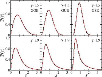
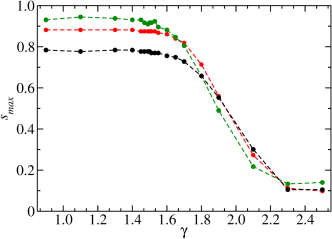
Figure 1: Left: Examples for the nearest-neighbor spacing distributions obtained from random-matrix simulations for the gRP model (black histograms) for the transition from Poisson to GOE (left column), GUE (middle column) and GSE (right column), respectively. They are compared to the curves $P_{0\to\beta}(s)$ given in Eqs. (9-13) best fitting them (red dashed line). Right: Position of the maximum of the best-fitting $P_{0\to\beta}(s)$ as function of the transition parameter $\gamma$ for $\beta=1$ (black), $\beta=2$ (red) and $\beta=4$ (dark green).

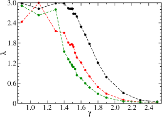
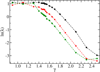
Figure 2: Left: Values of $\lambda$ obtained from the fit of $P_{0\to\beta}(s)$ to the numerical results for $\beta=1$ (black), $\beta=2$ (red) and $\beta=4$ (green) as function of $\gamma$. Right: Same as left for the natural logarithm of $\lambda$.

We also analyzed the distribution of the ratios of consecutive spacings [86, 87] between nearest-neighbor eigenvalues, $r_{j}=\frac{E_{j+1}-E_{j}}{E_{j}-E_{j-1}}$ and of $r_{j}^{min}=\rm{min}\left(r_{j},\frac{1}{r_{j}}\right)$. Wigner-surmise like analytical expressions are available for all three WD ensembles [87, 88]. They are applicable to systems for which the spectral density does not exhibit singularities and have the advantage that no unfolding is required, since the ratios are dimensionless [86, 87, 88].

Based on the joint probability distribution (A27) of the eigenvalues of $\hat{H}^{0\to 2}(\lambda)$ for the transition from Poisson to GUE, we derive in Sec. A.2 a Wigner-surmise like analytical expression for the ratio distribution, which is given in (A76). Examples are shown in Fig. A1. With increasing $\lambda$ a transition from the result (A48) for the eigenvalues of a $3\times 3$-dimensional diagonal matrix with Gaussian distributed entries to (A86) for the Wigner-surmise like analytical result for the GUE takes place. In Fig. 3 we compare for a few values of $\gamma$ the numerical results to the corresponding analytical ones. Like for the Wigner-surmise like results for the nearest-neighbor spacing distributions the numerical evaluation of (A76) becomes increasingly cumbersome with increasing $\gamma$, because in the limit $\lambda\to 0$ ($\gamma\to\infty$) the integrand turns into a $\delta$-function as outlined in the appendix [see (A44)], reflecting the abrupt transition of the ratio distribution occurring when increasing $\lambda$ from zero to any small value in (1) [74, 32].

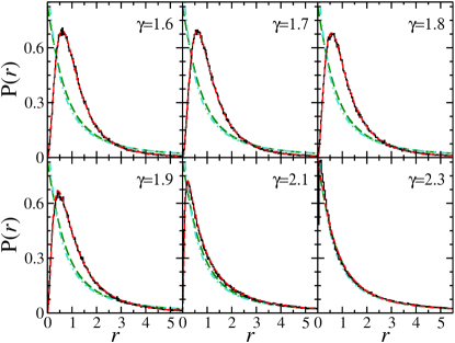
Figure 3: Examples for ratio distributions obtained from random-matrix simulations for the gRP model (black histograms) for the transition from Poisson to GUE. They are compared to the corresponding analytical result obtained from  (A76) (red dashed line). The turquoise dash-dot-dot lines show the analytical result (A49) for Poissonian distributed random numbers [87], the dashed green line the result for $3\times 3$-dimensional diagonal matrices with Gaussian distributed entries given in (A48). For $\gamma=1.6$ the curve is close to the Wigner-surmise like distribution of the GUE (A86). For $\gamma=2.3$ the numerical result is closer to the distribution (A48) than to the curve for Poissonian random numbers (A49).

For all three WD ensembles analytical results have been obtained for $\langle r\rangle$ and $\langle r^{min}\rangle$ [88], $\langle r\rangle=1.75,1.36.1.17$ and $\langle r^{min}\rangle=0.53,0.6,0.67$ for the GOE, GUE and GSE, respectively, and for Poissonian random numbers they are given by $\langle r\rangle=\infty$ and $\langle r^{min}\rangle=0.39$. These values are attained for $\beta=1,2,4$ in the limits of small and large $\gamma$, respectively. This is illustrated in Fig. 4, where we also show the analytical result as blue solid line for the transition from Poisson to GUE. Marginal deviations from the results for the WD ensembles are observed for $\lambda\gtrsim 1.45$, however, clear changes occur only above $\lambda\gtrsim 1.6$, thus implying that the ratio distributions are even less sensitive to small perturbations of the WD matrices [58, 60] than the nearest-neighbor spacing distribution. Nevertheless, they are commonly used to get information on presence or absence of quantum chaos, respectively, ergodicity, the reason being that no unfolding of the eigenvalues is required. In Fig. 5 we show for all three WD ensembles the average values $\langle r^{min}\rangle$ for different system sizes $N$. We observe for all cases ($\beta=1,2,4$) a crossing of the curves at $\gamma=2$, implying that at that value $\langle r^{min}\rangle$ does not depend on $N$. This indicates that a phase transition from extended to localized takes place at $\gamma=2$ [58]. Remarkably, the transition takes place at the same value of $\gamma$ for all three universality classes. Figure A4 exhibits $\langle r^{\rm min}\rangle$ as function of $\gamma$ and of the center of a sliding energy window comprising 500 eigenvalues for all three WD ensembles. The plots clearly show an energy dependent transition from WD to Poisson statistics, thus indicating a mobility edge for the associated eigenvectors.

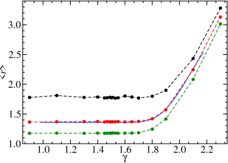
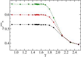
Figure 4: Average values for $\langle r\rangle$ (left) and $\langle r^{min}\rangle$ (right) for the transitions from Poisson to the WD ensembles (black: $\beta=1$, red: $\beta=2$, green: $\beta=4$) as function of $\gamma$. The blue line exhibits the corresponding analytical result. Note, that the ratio distribution (A76) becomes indistinguishable from the result (A48) (except for $\lambda<r$) for $\gamma\gtrsim 2.1$, so we don’t show results above that value.

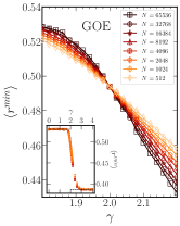
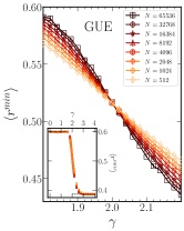
Figure 5: System size dependence of the average values $\langle r^{min}\rangle$ for transitions from Poisson to the WD ensembles as a function of $\gamma$. The insets show the extended $\gamma$ region for four system sizes, with the ergodic and Poisson values marked by dashed black lines.

II.2 Long-range correlations

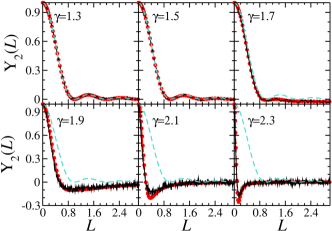
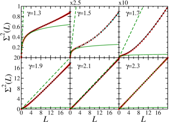
Figure 6: Left: Comparison of the two-point cluster function obtained from the random-matrix simulations for the GUE gRP Hamiltonian (2) (black) with the analytical result (A87) (red) for various values of $\gamma$ indicated in the panels. Here, $L$ denotes the length of the energy interval in units of mean spacing. The dashed turquoise line exhibits the result for the WD ensemble with $\beta=2$. Right: Comparison of the number variance obtained from the random-matrix simulations for the GUE gRP Hamiltonian (2) (black) with the analytical result (A88) (red) for various values of $\gamma$ indicated in the panels. The turquoise line shows one example for random matrices of dimension $N=100000$. It is indistinguishable from the result for $N=2^{16}$. The solid and dashed green lines exhibit the results for Poisson and GUE statistics, respectively.

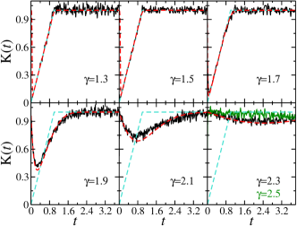
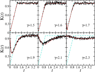
Figure 7: Left: Comparison of the spectral form factor obtained from the random-matrix simulations for the GUE gRP Hamiltonian (2) (black) with the analytical result (A.3) (red) for various values of $\gamma$. The corresponding values of $\lambda$ are obtained by fitting the analytical curves to the numerical ones. We do not show them, since they agree with the values obtained from the nearest-neighbor spacing distributions. Right: Same as in the left panel, the only difference being that the analytical curve is obtained from the Fourier transform of the analytical result (A87) for the two-point cluster function (red). Some slight discrepancies are observed for small values of $t$ for the case $\gamma=1.7$, but otherwise agreement with the numerical ones is as good as in the left panel, if not better.

Based on the RP model (1), in Ref. 32 approximate analytical results were obtained for the two-point cluster function for the transition from Poisson to GOE and an analytical expression for the transition from Poisson to GUE, which is exact for all values of $\lambda$ and $N$, however, the computation of the limit $N\to\infty$ starting from that expression was impossible [32]. In [89] the replica approach was applied to the gRP model for the transition from Poisson to GOE to compute the average spectral density and level compressibility. Yet, exact analytical results for statistical measures of long-range correlations of random matrices from the RP ensemble (1) are only available for $\beta=2$, see Appendix A.3. Examples for the two-point cluster function and number variance are shown in Fig. 6, and for the spectral form factor in the left panel of Fig. 7. The values of $\lambda$ obtained from the fit of the analytical result for $\Sigma^{2}(L)$ to the numerical results as function of $\gamma$ agree with those obtained from the fit of $P_{0\to 2}(s)$ given in (II.1) to the nearest-neighbor spacing distribution of the gRP Hamiltonian (2) with $\beta=2$ shown in Fig. 2. Note, that there are discrepancies in the scales of $\tilde{\alpha}$ and $\tilde{\tau}$ between Refs. [48] and [73]. These are due to differing definitions of the $N$-dependent scale of the parameter $\lambda$. We fixed this by computing the spectral form factor from the Fourier transform of the analytical result for the two-point cluster function [73] given in (A87) (right panel of Fig. 7) and comparing it to the analytical result for $K(\tau)$ [48] given in (A.3) (left panel of Fig. 7). Furthermore, we compared the resulting values of $\tilde{\alpha}$ and $\tilde{\tau}$ with those obtained from the fits of the Wigner-surmise like analytical result, $P_{0\to 2}(s)$, to the nearest-neighbor spacing distributions obtained for the gRP model, shown in Fig. 2, yielding $\tilde{\alpha}=\frac{\pi}{\sqrt{2}}\lambda$ and $\tilde{\tau}=\frac{\tau}{2\pi}$. For the matter of completeness, we would like to mention, that approximations have been derived for $Y_{2}^{0\to 2}(r)$ for $\lambda\ll 1$ and $\lambda\gg 1$ in Refs. 90, 91, 32, 47, 45, 71, 34, 72, 92, 48, 73.

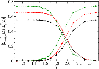
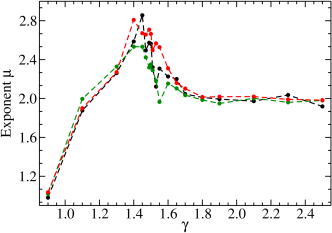
Figure 8: Left: Distance between the number variance $\Sigma^{2}(L)$ at $L=3$ for $\gamma=0.9$, where it coincides with that for the corresponding WD ensemble (dots), respectively, for Poisson statistics (triangles) and its value for $\gamma>0.9$ for the transition from Poisson to GOE (black), to GUE (red) and to GSE (green). Right: Same as left for the exponent $\mu$ deduced from the logarithm of power spectra, $\log_{10}[s(\tau)]$ as function of $\log_{10}[\tau]$ in the asymptotic region $\tau\lesssim 10^{-2}$ (see main text).

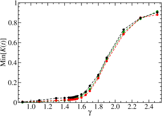
Figure 9: Left: Position $t_{min}$ of the minimum of the form factor $K(t)$ for the GOE (black), GUE (red) and GSE (green). Right: Same as left for the value of the form factor at the position of the minimum, $K(t_{min})$.

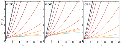
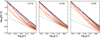
Figure A5: Left: Number variance $\Sigma^{2}(L)$ obtained from random-matrix simulations for the gRP model for $\beta=2$ (left), $\beta=1$ (middle) and $\beta=4$ (right) for the same values of $\gamma$ and color coding as in Fig. A3. The color changes from yellow to brown with increasing $\gamma$ and $\Sigma^{2}(L)$ experiences a transition from WD to Poisson. Actually, for $\gamma=0.9$ the curves lie on top of the WD result (turquoise dashed line), whereas already for $\gamma=1.1$ deviations are visible and for $\gamma=2.5$ they lie on top of the curve for Poissonian random numbers (turquoise dash-dot line). Right: Same as left for the power spectrum. For $\gamma=0.9$ the curve is close to an approximate result for the corresponding WD ensemble (turquoise dashed line), and for $\gamma=2.5$ it lies on top of the approximate result for Poissonian random numbers (turquoise dash-dot line) (see main text).

In the left part of  Fig. A5 results are shown for the number variance for the gRP Hamiltonian (2) with (3) for $\beta=1,2,4$. In Fig. A7 we show the numerical results for the spectral form factor for the gRP models with $\beta=1,4$. The turquoise lines show the results for the corresponding WD ensemble. For the two-point cluster functions, shown in the left part of Fig. 6, deviations from the WD ensemble with $\beta=2$ are visible only for $\gamma\gtrsim 1.5$, whereas clear discrepancies are observed in $\Sigma^{2}(L)$ for all values of $\beta$ for $\gamma\gtrsim 1$. To illustrate this, we plot in the left part of Fig. 8 its distance from the curve for $\gamma=0.9$, which lies on top of the WD one, at $L=3$ (dots), and similarly, the distance from Poisson statistics (triangles). For $\gamma\gtrsim 1$ the distances are nonzero for the former and they increase rapidly for $\gamma\gtrsim 1.4$ and saturate for $\gamma\gtrsim 2$ and are close to Poisson then. For the spectral form factor slight deviations from the corresponding WD ensemble are observed for $\gamma\gtrsim 1$ around the minimum at $t\simeq 0$, and for $\gamma\gtrsim 1.5$ discrepancies between the gRP and WD ensembles are clearly visible. To illustrate this, we plot in Fig. 9 the value of $t$ at the minimum of $K(t)$ (left), denoted by $t_{min}$, and the value of the minimum, $K(t_{min})$, itself. In the ergodic limit both values are zero, whereas for Poissonian random numbers the spectral form factor is constant, $K(t)=1$, and thus doesn’t exhibit a minimum. We find that $t_{min}$ and $K(t_{min})$ are nonzero for $\gamma\gtrsim 1$ and for $\gamma\gtrsim 2$ they increase drastically and $K(t_{min})$ saturates at about unity.

Another measure for long-range correlations is the power spectrum defined in (8). Exact analytical results were obtained for the power spectra in Refs. 93, 94 for fully chaotic quantum systems with violated ${\mathcal{T}}$-invariance, however, we are not aware of any analytical results for the RP model. The power spectrum exhibits for $\tau\ll 1$ a power law behavior $\langle s(\tau)\rangle\propto\tau^{-\mu}$, where $\mu=2$ for Poisson distributed random numbers and $\mu=1$ independently of the universality class for the WD ensembles. In the right part of Fig. A5 we show logarithmic plots of the power spectra versus $\log_{10}[\tau]$ obtained from the gRP model for all three universality classes. They are compared to theoretical approximations in terms of the spectral form factor derived in Ref. 95 for the WD ensembles and Poisson statistics, that have been tested experimentally for all WD ensembles [30, 96] for spectra consisting of several hundreds of eigenvalues.

In Fig. A6 we compare the approximation obtained from the analytical results for the spectral form factor to the numerical results for the power spectrum for several values of $\gamma$. There are deviations especially for $1.4\lesssim\gamma\lesssim 1.7$. Even for $\gamma=0.9$, which is close to the GUE curve, slight differences are visible. We attribute this to the high dimensions of the matrices used, that are large enough to reveal deviations from the approximations. Furthermore, these figures illustrate that the power spectra indeed increase linearly with decreasing $\log_{10}[\tau]$ for $\log_{10}[\tau]\lesssim-1.6$ for $\beta=4$ and for $\log_{10}[\tau]\lesssim-2$ for $\beta=1,2$. For $\gamma\gtrsim 1$ their slopes change drastically with increasing $\gamma$ and approach the result for Poisson statistics for $\gamma\gtrsim 2$. Accordingly, we may use the slope of the straight line best fitting $\log_{10}\left[s\left(\tau\right)\right]$ for $\log_{10}[\tau]\lesssim-2$ as indicator for the onset of deviations from WD statistics and agreement with Poisson. We show the values of $\mu$ obtained from linear regression of the logarithm of the power spectra as function of the logarithm of $\tau$ for $\tau\lesssim 10^{-2}$ for the three WD ensembles in the right part of Fig. 8. Deviations from WD statistics are visible for $\gamma>1$ and at $\gamma\simeq 1.45$ an abrupt change is observed. For $\gamma\gtrsim 1.9$ the random-matrix curves agree with the result for Poissonian random numbers.

Summarizing the results of Sec. II, we observe in the short-range correlations changes in the position of the maximum of the nearest-neighbor spacing distributions and the average ratio distributions above $\gamma\approx 1.45-1.6$ and saturation above $\gamma\simeq 2$, whereas in the long-range correlations changes are visible for $\gamma\gtrsim 1$. Yet, for $\gamma\gtrsim 2$ deviations of $\Sigma^{2}(L)$ from the corresponding WD curve, the power $\mu$ of the asymptotic algebraic decay of the power spectrum and the position of the minimum of the form factor saturate at values close to those of Poissonian random numbers.

III Properties of the eigenvectors of the gRP model

Long-range correlations like the number variance and the spectral form factor clearly indicate the ergodic transition, however for the unambiguous determination of the fractal phase and the Anderson transition, the analysis of properties of the eigenvectors of the gRP Hamiltonian $\hat{H}^{\rm gRP}(\gamma)$ in (2) is needed. In this section we investigate them in terms of fractal dimensions [44], participation ratios [46] and participation entropy [58], Kullback-Leibler divergences [97, 58, 67] and fidelity susceptibility [98, 61]. Due to Kramer’s degeneracies for the gRP model with symplectic universality class, we only consider one half of the eigenvectors, namely those with an odd index, for that case.

III.1 Fractal dimensions

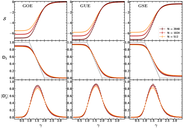
Figure 10: Participation entropy ${\cal{S}}$, fractal dimension $D_{1}$ and the derivative of fractal dimension $|D_{1}^{\prime}|$ for the GOE, GUE and GSE gRP model for system sizes $N=2^{n}$, with $n=9,10,11$ (yellow to brown). The dotted line in the fractal dimension is the analytical result [44].

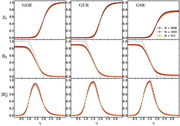
Figure 11: Participation number ${\cal{I}}_{2}$, fractal dimension $D_{2}$ and the derivative of fractal dimension $|D_{2}^{\prime}|$ for the GOE, GUE and GSE gRP model for system sizes $N=2^{n}$, with $n=9,10,11$ (yellow to brown). The dotted line in the fractal dimension is the analytical result [44].

We analyzed several measures to obtain information on the properties of the eigenvectors, one being the generalized participation numbers (PN):

$${\cal{I}}_{q}=\langle\sum_{i}|\psi_{\mu}(i)|^{2q}\rangle,$$ (14)

where the normalized $\mu-$th eigenstate of the Hamiltonian, $H|\psi_{\mu}\rangle=E_{\mu}|\psi_{\mu}\rangle$, is written in the computational basis $|\psi_{\mu}\rangle=\sum_{i}\psi_{\mu}(i)|i\rangle$, and the average is taken over a chosen energy window around the band center as well as over multiple disorder realizations. From the generalized PN we extract the fractal dimensions as

$$D_{q}=\log_{N}({\cal{I}}_{q})/(1-q).$$ (15)

For $q=1$ it yields the participation entropy,

$${\cal{S}}=\langle\sum_{i}|\psi_{\mu}(i)|^{2}\log(|\psi_{\mu}(i)|^{2})\rangle=-D_{1}\log(N)+const.$$ (16)

For the localized, fractal and extended phases the values of the fractal dimensions are $D_{q}=0$, $0<D_{q}<1$, and $D_{q}=1$, respectively. In Figs. 10 and 11 we show for all three WD ensembles the participation entropy and participation numbers for dimensions $N=2^{n},\ n=9,10,11$ together with $D_{1}$ and $D_{2}$, respectively. For $D_{1}$ and $D_{2}$ we also show the analytical result $D_{q}=1,2-\gamma,0$ for $\gamma<1$, $1<\gamma<2$ and $\gamma>2$, respectively, derived in Ref. 44 for the transitions from Poisson to GOE and GUE. We also plot it for the transition to GSE. Deviations between the analytical curve and numerical results are of the same size for the unitary and symplectic universality classes for $1\leq\gamma\lesssim 2$. However, for $\gamma\gtrsim 2$ $D_{1}$, $D_{2}$ and ${\cal{S}}$ approach a non-zero value and, accordingly, ${\cal{I}}_{2}$ is less than unity for the symplectic case. Note that, due to Kramer’s degeneracy the dimension is effectively one half of that of the other two cases. More importantly, any linear combination of the associated eigenvectors are eigenvectors of $\hat{H}^{\rm gRP}$ in (2), so that the occupation probabilities are spread over two eigenstates. This explains, why for these measures the values expected for complete localization are not yet attained for the highest considered dimension and $q$ value.

The ergodic and Anderson transitions are identified in the corresponding derivatives $|D_{1}^{\prime}|$ and $|D_{2}^{\prime}|$ as the values of $\gamma$, where the curves for different $N$ cross. These values agree well with the predicted values $\gamma_{E}=1$ and $\gamma_{A}=2$, respectively [58]. Note, that the positions of the maxima of $|D_{1}^{\prime}|$ and $|D_{2}^{\prime}|$, that is of the turning points of $D_{1}$ and $D_{2}$, as function of $\gamma$ are at the value $\gamma\simeq 1.5$, where deviations from the WD ensembles and drastic changes set in for the short-range correlations (see Figs. 1 and 4) and long-range correlations (see Figs. 8 and 9), respectively.

III.2 Kullback-Leibler divergence

The Kullback-Leibler (KL) divergence [97] or relative entropy is commonly used as a measure to compare two probability densities, exhibiting nonzero values when they differ, and values close to zero when they are similar. In our case the probability density of interest is that of the eigenstate occupations $|\psi_{\mu}(i)|^{2}$. The KL divergences that we study are defined as [58, 67]

$${\cal{K}}_{A}=\langle\sum_{i}|\psi_{\mu}(i)|^{2}\log(\frac{|\psi_{\mu}(i)|^{2}}{|\psi_{\mu+1}(i)|^{2}})\rangle$$ (17)

$${\cal{K}}_{E}=\langle\sum_{i}|\psi_{\mu}(i)|^{2}\log(\frac{|\psi_{\mu}(i)|^{2}}{|\tilde{\psi}_{\mu^{\prime}}(i)|^{2}})\rangle.$$ (18)

Here, ${\cal{K}}_{A}$ compares the occupation probability density of two eigenstates corresponding to nearest-neighbor eigenvalues within the same disorder realization and, accordingly, provides an appropriate measure to determine the Anderson localization phase transition, whereas ${\cal{K}}_{E}$ compares the distributions of two eigenstates from different realizations and yields a suitable indicator of the ergodic phase transition.

To determine the two transition points and the corresponding critical exponents we use the finite size scaling (FSS) analysis as described in Ref. 99. The KL divergences are assumed to be given by a scaling law

$${\cal{K}}_{l}=F(\Phi_{1},\Phi_{2}),$$ (19)

with the scaling variables $\Phi_{1},\Phi_{2}$, given as

$$\Phi_{j}=u_{j}(w)\bigl{[}\log(N)\bigr{]}^{\alpha_{j}},$$ (20)

where $w=(\gamma-\gamma_{c})/\gamma_{c}$ is the reduced parameter of the gRP model and $\gamma_{c}$ is the transition point to be determined. The logarithmic system size dependence in the scaling variables was first used in Ref. 58 and further justified in Ref. 67 and the corresponding scaling exponent are $\alpha_{1}$ and $\alpha_{2}$. For the relevant variables , $\Phi_{1}$, and the irrelevant ones, $\Phi_{2}$, the scaling exponents are given in terms of $\nu$ and $y$, respectively, with $\alpha_{1}=1/\nu$ and $\alpha_{2}=y$. In the vicinity of the transition the functions $u_{i}$ are Taylor expanded

$$u_{i}(w)=\sum_{j=0}^{m_{j}}b_{i,j}w^{j},$$ (21)

where the cutoff integer $m_{j}$ is a parameter of the FSS and $b_{i,j}$ are additional fitting coefficients. Similarly the scaling function $F$ is Taylor expanded in powers of the scaling variables

$$F(\Phi_{1},\Phi_{2})=\sum_{j_{1}=0}^{n_{1}}\sum_{j_{2}=0}^{n_{2}}a_{j_{1},j_{2}}\Phi_{1}^{j_{1}}\Phi_{2}^{j_{2}},$$ (22)

with fitting coefficients $a_{j_{1},j_{2}}$. To avoid disambiguity we set $a_{1,0}=a_{0,1}=1$ and $b_{1,0}=0$. Then the total number of free parameters is $N_{P}=2+m_{1}+m_{2}+(n_{1}+1)(n_{2}+1)$ and in order to determine them we minimize the $\chi^{2}$ statistics, given as

$$\chi^{2}=\sum_{l=1}^{N_{D}}\frac{(F_{l}-{\cal{K}}_{l})^{2}}{\sigma_{l}^{2}}.$$ (23)

In the numerical analysis, the ${\cal{K}}_{l}$ are obtained for matrix sizes $N=512-32768$: (i) for ${\cal{K}}_{E}$ by extracting a single state closest to the energy 0 and averaging over multiple realization of the gRP matrices; (ii) for ${\cal{K}}_{A}$ by averaging KL divergence values at different parameters $\gamma$ over $\pm 10\%$ of the $N$ eigenstates around the band center, which is at energy zero, and then averaging the resulting mean values over multiple realizations of gRP matrices. We find that the values ${\cal{K}}_{E}$ for nearby states within the same random matrix realization are highly correlated. Thus we take a single state closest to the band center from each realization. The associated standard errors of the mean yield $\sigma_{l}$ entering (23). The total number of data points is $N_{D}$. The results are shown in Figs. 12 and 13 (symbols) together with the curves best fitting them (solid lines of corresponding color). For the minimization of Eq. (23) we use the Levenberg–Marquardt (LM) algorithm as implemented in the LMFIT package in Python. We have also performed Monte-Carlo (MC) simulations of the synthetic data sets (as described in Ref. 100, Chapter 15.6) using $300$ to $1000$ sets.

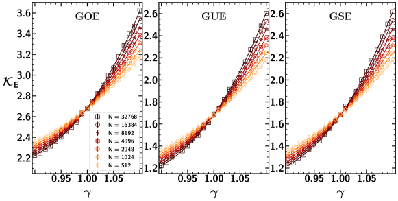
Figure 12: The KL divergence ${\cal{K}}_{E}$ near the ergodic transition for all three WD symmetry classes. The lines are the best fits obtained using the minimization of the $\chi^{2}$ statistics with $n_{1}=3,m_{1}=2,n_{2}=m_{2}=0$, see also Table 1.

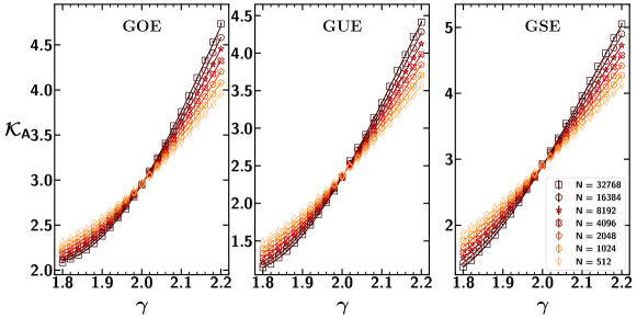
Figure 13: The KL divergence ${\cal{K}}_{A}$ near the Anderson transition for all three WD symmetry classes. The lines are the best fits obtained using the minimization of the $\chi^{2}$ statistics with $n_{1}=3,m_{1}=2,n_{2}=m_{2}=0$, see also Table 2.

The results of the fitting procedure are summarized in Tables 1 and 2 for the ergodic and Anderson transitions, respectively. For the ergodic transition the fitting without the irrelevant scaling variable gives consistent results with very high precision. For the GUE and GSE the irrelevant scaling variable is needed at the Anderson transition, as indicated by high values of $\chi^{2}$ if it is not used. We find that the stability of fitting is better for the ergodic transition. We suspect that this is due to the underestimation of $\sigma_{l}$ in Eq. (23), which might originate from the correlations between the fractal states within the same disorder realization as reported in Ref. 44 and is known to occur for the Anderson transition in the 3D Anderson model [101, 102]. Errors are largest for the GSE case, which we again attribute to Kramer’s degeneracy, implicating halving of the dimension and the superposition of the associated pairs of eigenmodes. Nevertheless the fitting results as given in Tables 1 and 2 agree very well for the different settings and clearly confirm up to the errors the prediction $\nu_{A}=\nu_{E}=1$, thus showing the superuniversality of the transitions in the gRP models.

class	$n_{1},m_{1},n_{2},m_{2}$	$\gamma_{E}$	$\nu_{E}$	$\chi^{2}$	$N_{D}$	MC sets
	$3,2,0,0$	$0.9971\pm 0.0006$	$1.0243\pm 0.0091$	147.4	147
GOE	$3,2,0,0$	$0.9971\pm 0.0007$	$1.0244\pm 0.0090$			1000
	$2,4,0,0$	$0.9965\pm 0.0006$	$1.0037\pm 0.0078$	154.0	147
	$2,4,0,0$	$0.9965\pm 0.0005$	$1.0035\pm 0.0076$			1000
	$3,2,0,0$	$0.99937\pm 0.00036$	$1.0032\pm 0.0051$	189.8	147
GUE	$3,2,0,0$	$0.99937\pm 0.00031$	$1.0032\pm 0.0044$			1000
	$2,4,0,0$	$0.99924\pm 0.00034$	$0.9997\pm 0.0053$	189.4	147
	$2,4,0,0$	$0.99924\pm 0.00028$	$0.9998\pm 0.0045$			1000
	$3,2,0,0$	$1.00192\pm 0.00040$	$1.0046\pm 0.0053$	203.6	147
GSE	$3,2,0,0$	$1.00192\pm 0.00045$	$1.0047\pm 0.0044$			1000
	$2,4,0,0$	$1.00091\pm 0.00035$	$0.9877\pm 0.0054$	213.8	147
	$2,4,0,0$	$1.00092\pm 0.00028$	$0.9876\pm 0.0043$			1000

Table 1: The FSS analysis for the ergodic transition in the gRP models for all three WD symmetry classes. The parameter range $\gamma\in[0.9,1.1]$ was used. The rows where $\chi^{2}$ and the number of MC sets are given show the results from the LM algorithm and the MC simulations, respectively. A single state closest to the band center was used per realization.

class	$n_{1},m_{1},n_{2},m_{2}$	$\gamma_{A}$	$\nu_{A}$	y	$\chi^{2}$	$N_{D}$	MC sets
	$3,2,0,0$	$2.0025\pm 0.0004$	$0.9964\pm 0.0032$		211.6	147
GOE	$3,2,0,0$	$2.0025\pm 0.0003$	$0.9966\pm 0.0026$				1000
	$5,2,0,0$	$2.0036\pm 0.0004$	$0.9984\pm 0.0029$		159.0	147
	$5,2,0,0$	$2.0035\pm 0.0004$	$0.9984\pm 0.0025$				1000
	$3,2,0,0$	$2.0068\pm 0.0005$	$0.9930\pm 0.0033$		404	147
GUE	$3,2,0,0$	$2.0068\pm 0.0003$	$0.9930\pm 0.0020$				1000
	$3,2,1,1$	$1.9989\pm 0.0021$	$1.0061\pm 0.0068$	$-5.7\pm 2.0$	$158.4$	147
	$3,2,1,1$	$1.9986\pm 0.0027$	$1.0062\pm 0.0068$	$-6.4\pm 2.6$			300
	$3,2,0,0$	$2.0020\pm 0.0007$	$0.9461\pm 0.0047$		1414	147
GSE	$3,2,0,0$	$2.0020\pm 0.0002$	$0.9461\pm 0.0014$				1000
	$3,2,1,1$	$1.965\pm 0.011$	$0.972\pm 0.035$	$-1.3\pm 0.7$	$203.1$	147
	$3,2,1,1$	$1.965\pm 0.008$	$0.970\pm 0.020$	$-1.4\pm 0.6$			300

Table 2: The FSS analysis for the Anderson transition in the gRP models for all three WD symmetry classes. The parameter range $\gamma\in[1.8,2.2]$ was used. The rows where $\chi^{2}$ and the number of MC sets are given show the results from the LM algorithm and the MC simulations, respectively. In total twenty percent of the states around the band center were used for each realization. Note that for $n_{2}=m_{2}=0$ no irrelevant scaling variables are used and thus $y$ equals zero.

III.3 Fidelity susceptibility

In Ref. 103 a new measure has been introduced which depends on the eigenvalues and eigenvectors of a parameter-dependent Hamiltonian, and probes ergodicity in terms of the adiabatic deformation of these eigenstates. The Hamiltonian is obtained by perturbing the gRP Hamiltonian $\hat{H}^{\rm gRP}(\gamma)$ in (2) with a parameter-dependent perturbation, $\hat{H}(\epsilon)=\hat{H}+\epsilon\hat{V}$. The adiabatic gauge potential (AGP) which generates the adiabatic deformation of the eigenstates $\{E_{l}(\epsilon),|l(\epsilon\rangle\}$ of $\hat{H}(\epsilon)$, obtained from the eigenvalue equation $\hat{H}(\epsilon)|l(\epsilon)\rangle=E_{l}(\epsilon)|l(\epsilon)\rangle$, is defined as

$$\mathcal{A}_{\epsilon}|l(\epsilon)\rangle=i\partial_{\epsilon}|l(\epsilon)\rangle.$$ (24)

Differentiation of the eigenvalue equation with respect to $\epsilon$ yields for $\epsilon\to 0$ [104, 78]

$$\langle m|A_{\epsilon}|l\rangle|_{\epsilon=0}=-i\frac{\langle m|\partial_{\epsilon}\hat{H}(\epsilon)|_{\epsilon=0}|l\rangle}{E_{m}-E_{l}},$$ (25)

where we introduced the notation $|l\rangle\equiv|l(\epsilon=0)\rangle$ and $E_{l}\equiv E_{l}(\epsilon=0)$. The Hilbert-Schmidt norm of $\langle m|A_{\epsilon}|l\rangle$ yields the fidelity susceptibility [105, 61],

$$\chi_{l}=\sum_{m\neq l}\frac{|\langle m|\partial_{\epsilon}\hat{H}(\epsilon)|_{\epsilon=0}|l\rangle|^{2}}{(E_{m}-E_{l})^{2}},$$ (26)

which has been shown [105, 103, 106, 107] to be a particularly sensitive measure for ergodicity. This can be expected from its structure. Namely, in the ergodic phase eigenfunctions are fully extended and the eigenvalues repel each other, whereas in the fractal phase eigenfunctions are partially localized [46] and part of the eigenvalues are nearly degenerate.

We consider an $\epsilon$-independent potential $\hat{V}$, which is diagonal in the representation of the unperturbed gRP Hamiltonian $\hat{H}^{\rm gRP}(\gamma)$ given in (2), with box-distributed random entries and compute for given $\hat{V}$ and matrix elements $H_{nm}$ in (3) the fidelity susceptibility $\chi$ as function of the gRP parameter $\gamma$. Here, we take into account $\pm 10\%$ of the eigenstates $|l\rangle$ around the band center for various dimensions $N$. Furthermore, we analyze the logarithm of $\chi_{l}$, $\zeta=\langle\langle\log(\chi_{l})\rangle_{l}\rangle_{\rm ens}$ to mitigate the accidental small denominators in the definition of $\chi_{l}$ [98], with $\langle\cdot\rangle_{l}$ and $\langle\cdot\rangle_{\rm ens}$ denoting the arithmetic mean over $l$ and ensemble average over numerous random-matrix realizations of $\hat{H}^{\rm gRP}(\gamma)$ defined in equations (2) and (3), respectively.

In Fig. 14 we show the fidelity susceptibility for the GOE gRP for $N=2^{n}$ with $n=9-15$. The number of realizations used was at least 2000, 1000, 500, 200, 100, 20, 3 for system sizes from 512 to 32768, respectively. In Fig. 15 we compare the results for the three WD ensembles for $n=9-11$, where less realizations were used for the GUE (500, 250, 50) and GSE (1000, 500, 100) classes. Due to the different random extensive observables used for different system sizes we rather compare $\zeta^{\prime}=\zeta(\gamma)-\zeta(\gamma=0)$. For all cases the curves for different dimensions $N$ cross each other at $\gamma=1$, indicating that there the transition from the ergodic to the fractal phase takes place. This is illustrated in Fig. 16 showing a zoom into the region around $\gamma=1$. For $\gamma>1$ the curves increase until they reach a maximum at $\gamma=2$, that is, at the value of $\gamma$ where the Anderson transition takes place. Beyond that value $\chi_{l}$ decreases to zero with increasing $\gamma$ for all WDs, indicating localization. Note, that the curves cross each other again at $\gamma\simeq 3$, however, in distinction to that at $\gamma=1$, there the crossings are spread over a nonzero range of $\gamma$ values.

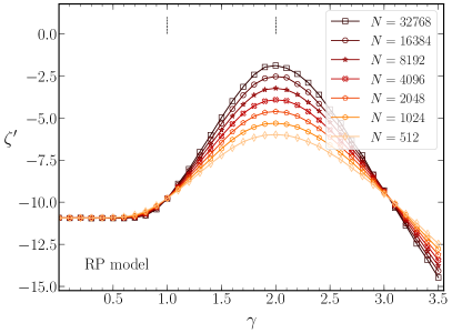
Figure 14: Fidelity susceptibility for the GOE gRP model using random extensive observable.

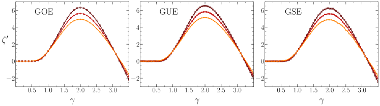
Figure 15: Fidelity susceptibility for the three WD gRP models using random extensive observable, for system sizes $N=512,1024,2048$. The curves were shifted vertically such that they all start at the same value $\zeta^{\prime}=0$ for $\gamma=0$.

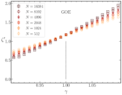
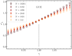
Figure 16: Fidelity susceptibility in the vicinity of the ergodic transition for the three WD gRP models using random extensive observable. The curves were shifted vertically such that they all start at the same value $\zeta^{\prime}=0$ for $\gamma=0$.

Conclusions

We analyzed spectral properties and properties of the eigenvectors of random matrices from the gRP model for all the WD ensembles. We extend the known results for the transition from Poisson to GOE and GUE to the symplectic universality class, i.e., the GSE. Furthermore, employing high-dimensional random matrices (N=65536), we validate for the transition from Poisson statistics to GUE the existing analytical results for the long-range correlations [48, 73] and an analytical expression for the ratio distribution derived in the appendix in Sec. A.2. We also compare for all three WD ensembles the numerically obtained nearest-neighbor spacing distributions to Wigner-surmise like results [74, 84]. We analyze the transition from extended to localized states in terms of the position of the maximum of the nearest-neighbor spacing distribution and the average ratios for short-range correlations. For long-range correlations, we employ the distance of the number variance from WD statistics, the asymptotic power-law behavior of the power spectrum and the position of the minimum of the spectral form factor to identify the transitions. We find that deviations from WD statistics are observed in the short-range correlations only above $\gamma\simeq 1.5$, whereas they set in immediately beyond $\gamma\simeq 1$ for the long-range correlations. Both the measures for short- and long-range correlations approach the corresponding result for Poissonian random numbers above $\gamma\simeq 2$ for all three WD ensembles.

To obtain information on the properties of the eigenvectors of the gRP Hamiltonian (2) and accurately determine the ergodic and Anderson transition and identify the fractal phase, we analyzed fractal dimensions, including the participation entropy and participation number, and KL divergences. For the symplectic case, due to Kramer’s degeneracy which implies that the occupation probability spreads over the pairs of eigenmodes associated with the degenerate eigenvalues, we find for the localized phase small deviations from the predicted values. The Anderson transition is seen in the generalized participation numbers, in addition the ergodic one in the derivative of the fractal dimensions $D_{1}$ and $D_{2}$. Both transitions are detected using KL divergences of eigenfunction occupations. A finite-size scaling analysis shows that all these measures show superuniversality of the transitions in the sense that the values of $\gamma_{E}$ and $\gamma_{A}$ are identical for all three WD ensembles, with the critical exponent being consistent with the value $\nu=1$. Similarly, the fidelity susceptibility detects the ergodic transition and exhibits a maximum at the Anderson transition. When looking at the curves for different dimensions $N$, shown in Figs. 14 and 15, one might conclude that there is a further transition at $\gamma=3$. However, there the curves do not cross at a single point and therefore they do not identify a genuine third transition.

One interesting question for future research is to confirm the ability of fidelity susceptibility to detect non-ergodic transitions by benchmarking it in other models with non-ergodic phases, and to investigate if (and how) it can discriminate between single fractal and multifractal regions in the parameter space. Another one is to find spectral measures for long-range correlations in addition to those considered in the present work that might provide useful indicators to detect transitions, e.g. non-ergodic ones.

Appendix A Analytical Results for the transition $\beta=0\to\beta=2$ from Poisson to GUE

A.1 The joint-probablity density of the eigenvalues for the transition from Poisson to GUE

The derivation of the joint-probability distribution of the eigenvalues $\{e_{i}\}$, $P(\{e_{i}\};\gamma)$ of random matrices from the RP model

$$\hat{H}^{0\to 2}(\lambda)=\hat{H}_{0}+\lambda\hat{H}^{(\beta=2)},\,\lambda=\frac{1}{N^{\gamma/2}},$$ (A27)

where $\hat{H}^{(0)}$ denotes a random diagonal matrix and $\hat{H}^{\beta}$ a random matrix from the GUE with $\beta=2$, with Gaussian distributed matrix elements with variances

$$\left\langle\left(H^{2}_{nm}\right)^{2}\right\rangle=\sigma^{2}=1.$$ (A28)

involves an integral over the unitary matrices diagonalizing it, which is the Harish-Chandra Itzykson-Zuber integral [108, 109, 32], yielding

$$P(\{e_{i}\})=\left(\frac{1}{\sqrt{2\pi\lambda^{2}}}\right)^{N}\int d\left[\bm{E}\right]P^{(0)}(\bm{E})\exp\left[-\frac{1}{2\lambda^{2}}\sum_{i}(e_{i}-E_{i})^{2}\right]\frac{\prod_{n<m}(e_{n}-e_{m})^{2}}{\prod_{n<m}(E_{n}-E_{m})^{2}}.$$ (A29)

The probablity density $P^{(0}(\bm{E})$ of the matrix elements $E_{i}$ of $\hat{H}^{0}$ is arbitrary, however for the numerical simulations we chose them Gaussian distributed with variances

$$\tilde{\sigma}^{2}=\left\langle\left(H^{0}_{nn}\right)^{2}\right\rangle=\sigma^{2}\left(1-\lambda^{2}\right),$$ (A30)

$$P^{(0}(\bm{E})=\prod_{i=1}^{N}\frac{e^{-E_{i}^{2}/2\tilde{\sigma}^{2}}}{\sqrt{2\pi\tilde{\sigma}^{2}}}.$$ (A31)

A.2 Derivation of the ratio distribution for the transition from Poisson to GUE

Starting from (A29), we derive a Wigner-surmise like expression for the distribution $P^{0\to 2}(r)$, abbreviated as $P(r)$ in the following, of the ratios $r_{i}=\frac{e_{i+1}-e_{i}}{e_{i}-e_{i-1}}$ of the sorted eigenvales $e_{i}\leq e_{i+1},i=1,\dots\,,N$ by restricting to $N=3$,

$$P(r)=3!\int_{-\infty}^{\infty}de_{2}\int_{-\infty}^{e_{2}}de_{1}\int_{e_{2}}^{\infty}de_{3}P(e_{1},e_{2},e_{3})\delta\left(r-\frac{e_{3}-e_{2}}{e_{2}-e_{1}}\right).$$ (A32)

We perform a variable transformation $[e_{1},e_{2},e_{3}]\rightarrow[\tilde{e}_{1}=e_{1}/(\sqrt{2}\lambda),\tilde{e}_{2}=e_{2}/(\sqrt{2}\lambda),\tilde{e}_{3}=e_{3}/(\sqrt{2}\lambda)]$, similarly $[E_{1},E_{2},E_{3}]\rightarrow[E_{1}/(\sqrt{2}\lambda),E_{2}/(\sqrt{2}\lambda),E_{3}/(\sqrt{2}\lambda)]$, and then $[\tilde{e}_{1},\tilde{e}_{2},\tilde{e}_{3}]\longrightarrow[x=(\tilde{e}_{2}-\tilde{e}_{1}),z,y=(\tilde{e}_{3}-\tilde{e}_{2})]$ yielding

$$P(r)= 3!\left(\sqrt{\frac{2\lambda^{2}}{\pi}}\right)^{3}\int_{-\infty}^{\infty}dE_{1}\int_{-\infty}^{\infty}dE_{2}\int_{-\infty}^{\infty}dE_{3}\frac{P_{3}^{(0)}(\sqrt{2}\lambda\bm{E})}{\Delta(\bm{E})}e^{-(E_{1}^{2}+E_{2}^{2}+E_{3}^{2})}$$ (A33)

$$\times \int_{0}^{\infty}dx\int_{0}^{\infty}dyxy(x+y)\exp\left[-\left(x^{2}+y^{2}\right)-2\left(xE_{1}-yE_{3}\right)\right]\delta\left(r-\frac{y}{x}\right)$$

$$\times \int_{0}^{\infty}dz\exp\left[-3z^{2}+2z\left(x-y+E_{1}+E_{2}+E_{3}\right)\right],$$

with $\Delta(\bm{E})=(E_{3}-E_{2})(E_{3}-E_{1})(E_{2}-E_{1})$. The integrations over $y$ and $z$ lead to

$$P(r)= 3!\frac{r(r+1)}{\sqrt{3}}\frac{2\lambda^{2}}{\pi}\int_{-\infty}^{\infty}dE_{1}\int_{-\infty}^{\infty}dE_{2}\int_{-\infty}^{\infty}dE_{3}\frac{P_{3}^{(0)}(\sqrt{2}\lambda\bm{E})}{\Delta(\bm{E})}e^{-(E_{1}^{2}+E_{2}^{2}+E_{3}^{2})}e^{(E_{1}+E_{2}+E_{3})^{2}/3}$$ (A34)

$$\times \int_{0}^{\infty}dxx^{4}\exp\left[-\frac{2}{3}(1+r+r^{2})x^{2}+\frac{2x}{3}\left(-2E_{1}+E_{2}+E_{3}\right)+r\left(2E_{3}-E_{1}-E_{2}\right)\right].$$

Next, we insert for $P_{3}^{(0)}(\bm{E})$ (A31), perform a variable change from $[E_{1},E_{2},E_{3}]\rightarrow[u=(E_{2}-E_{1}),w,v=(E_{3}-E_{2})]$ and introduce the notation $\alpha^{2}=\frac{\lambda^{2}}{1-\lambda^{2}}$, so that the integrals over $\{E_{i}\}$ become,

$$I= \int_{-\infty}^{\infty}\frac{du}{u}\int_{-\infty}^{\infty}\frac{dv}{v}\frac{1}{u+v}\exp\left\{-(\alpha^{2}+1)(u^{2}+v^{2})+\frac{(v-u)^{2}}{3}+\frac{2x}{3}\left[2u+v+r(2v+u)\right]\right\}$$ (A35)

$$\times \int_{-\infty}^{\infty}dwe^{\left[-3\alpha^{2}w^{2}+2w(u-v)\alpha^{2}\right]}\left[\frac{1}{\sqrt{2\pi(1-\lambda^{2})}}\right]^{3}.$$ (A36)

Performing the integral over $w$ yields

$$P(r)= 2r(r+1)\frac{\alpha^{2}}{\pi^{2}}\int_{-\infty}^{\infty}\frac{du}{u}\int_{-\infty}^{\infty}\frac{dv}{v}\frac{1}{u+v}\exp\left[-\frac{2}{3}(\alpha^{2}+1)(u^{2}+v^{2}+uv)\right]$$ (A37)

$$\times \int_{0}^{\infty}dxx^{4}\exp\left[-Rx^{2}+2xF\right],$$ (A38)

where we introduced the notations

$$R=\frac{2}{3}(1+r+r^{2}),\,F(u,v)=\frac{1}{3}[2u+v+r(u+2v)].$$ (A39)

Integration over $x$ leaves us with a double integral,

$$P(r)=2r(r+1)\frac{\alpha^{2}}{\pi^{2}}\int_{-\infty}^{\infty}\frac{du}{u}\int_{-\infty}^{\infty}\frac{dv}{v}\frac{1}{u+v}\exp\left[-\frac{2}{3}(\alpha^{2}+1)(u^{2}+v^{2}+uv)\right]g(u,v)$$ (A40)

with

$$g(u,v)=\frac{1}{2R}\left(\frac{F}{R}\right)^{3}+\frac{5}{4R^{2}}\frac{F}{R}+e^{\frac{F^{2}}{R}}\frac{1}{2}\sqrt{\frac{\pi}{R}}\left[1+\Phi\left(\frac{F}{\sqrt{R}}\right)\right]\left\{\frac{3}{4R^{2}}+\frac{3}{R}\left(\frac{F}{R}\right)^{2}+\left(\frac{F}{R}\right)^{4}\right\}.$$ (A41)

Here, $\Phi(x)$ denotes the error function. Due to the symmetry properties of the integrand, terms with $g(u,v)=g(-u,-v)$ and $g(u,-v)=g(-u,v)$ cancel each other, so that the first term in the square bracket in (A41) vanishes upon integration.

Before we continue with the integration we consider the limit $\alpha\to 0$. For this we introduce the variable transformation $[u,v]\to[\tilde{u}=\alpha u,\tilde{v}=\alpha v]$, resulting with $\tilde{F}(\tilde{u},\tilde{v})=\alpha F(u,v)$ in

$$P(r)=\frac{2r(r+1)}{\pi^{2}}\int_{-\infty}^{\infty}\frac{du}{u}\int_{-\infty}^{\infty}\frac{dv}{v}\frac{1}{u+v}\exp\left[-\frac{2}{3}\left(1+\frac{1}{\alpha^{2}}\right)(u^{2}+v^{2}+uv)\right]$$ (A42)

$$\times\left\{\frac{1}{2R}\left(\frac{\tilde{F}}{R}\right)^{3}+\alpha^{2}\frac{5}{4R^{2}}\frac{\tilde{F}}{R}+e^{\frac{\tilde{F}^{2}}{\alpha^{2}R}}\frac{1}{2}\sqrt{\frac{\pi}{R}}\Phi\left(\frac{\tilde{F}}{\alpha\sqrt{R}}\right)\left[\alpha^{3}\frac{3}{4R^{2}}+\frac{3}{R}\alpha\left(\frac{\tilde{F}}{R}\right)^{2}+\frac{1}{\alpha}\left(\frac{\tilde{F}}{R}\right)^{4}\right]\right\}.$$ (A43)

In the limit $\alpha\to 0$ only the last term in the curly bracket remains and we obtain with

$$\frac{1}{\alpha}\exp\left[-\frac{1}{\alpha^{2}}\left(\frac{2}{3}(u^{2}+v^{2}+uv)-\frac{\tilde{F}^{2}}{R}\right)\right]\xrightarrow{\alpha\to 0}\sqrt{\pi}\delta\left(\sqrt{\frac{2}{3}(u^{2}+v^{2}+uv)-\frac{\tilde{F}^{2}}{R}}\right),$$ (A44)

$$P(r)=\sqrt{\pi}\frac{2r(r+1)}{\pi^{2}}\int_{-\infty}^{\infty}\frac{du}{u}\int_{-\infty}^{\infty}\frac{dv}{v}\frac{1}{u+v}\exp\left[-\frac{2}{3}(u^{2}+v^{2}+uv)\right]$$ (A45)

$$\times\sqrt{3R}\delta\left(v-ur\right)\frac{1}{2}\sqrt{\frac{\pi}{R}}\frac{\tilde{F}}{|\tilde{F}|}\left(\frac{\tilde{F}}{R}\right)^{4}$$ (A46)

$$=\frac{\sqrt{3}}{\pi}\int_{0}^{\infty}du2ue^{-Ru^{2}}$$ (A47)

$$=\frac{\sqrt{3}}{R\pi}=\frac{3\sqrt{3}}{2\pi(1+r+r^{2})},$$ (A48)

which is the Wigner-surmise like result for the ratio distribution of the Gaussian-distributed elements $E_{i}$ with arbitrary variance $\sigma^{2}$ of the diagonal matrix $\hat{H}_{0}$ in (A27). It differs from the result for Poissonian random numbers,

$$P^{\rm Poi}(r)=\frac{1}{(1+r)^{2}}.$$ (A49)

Next we compute the integral in (A40) for $\alpha>0$. In order to get rid of the factor $1/(u+v)$ in (A40), we use

$$\frac{F}{uv(u+v)}=\frac{(2+r)}{v(u+v)}+\frac{(1+2r)}{u(u+v)},$$ (A50)

and define new integration variables $[\tilde{u}=(u+v),\tilde{v}=v]$ for the first term and $[\tilde{u}=u,\tilde{v}=(u+v)]$ for the second one. Introducing polar coordinates $[\tilde{u}=\rho\cos\varphi,\tilde{v}=\rho\sin\varphi]$ and the notations

$$F_{1}(\varphi)=\frac{1}{3\sqrt{R}}\left|(2+r)\cos(\varphi/2)+(r-1)\sin(\varphi/2)\right|$$ (A51)

$$F_{2}(\varphi)=\frac{1}{3\sqrt{R}}\left|(r+1)\cos(\varphi/2)+(1+2r)\sin(\varphi/2)\right|$$ (A52)

leads to

$$P(r)=4\frac{r(r+1)}{R^{3}}\frac{\alpha^{2}}{\pi^{2}}\int_{-\pi}^{\pi}\frac{d\varphi}{\sin\varphi}\int_{0}^{\infty}d\rho\exp\left[-\frac{2}{3}(\alpha^{2}+1)\rho^{2}\left(1-\frac{\sin\varphi}{2}\right)\right]h(\varphi,\rho)$$ (A53)

with

$$h(\varphi,\rho) =\frac{f(\varphi)}{2}\rho+\frac{5}{4}\frac{1+r}{\rho}$$ (A54)

$$+e^{F_{1}^{2}\rho^{2}}\frac{\sqrt{\pi}}{2}\Phi\left(F_{1}\rho\right)\left[\frac{3}{4}\frac{1}{F_{1}}\frac{1}{\rho^{2}}+3F_{1}+\left(F_{1}\right)^{3}\rho^{2}\right]\frac{2+r}{3}$$ (A55)

$$+e^{F_{2}^{2}\rho^{2}}\frac{\sqrt{\pi}}{2}\Phi\left(F_{2}\rho\right)\left[\frac{3}{4}\frac{1}{F_{2}}\frac{1}{\rho^{2}}+3F_{2}+\left(F_{2}\right)^{3}\rho^{2}\right]\frac{1+2r}{3}\,$$ (A56)

and

$$f(\varphi) =\left[\frac{2+r}{3}F_{1}^{2}+\frac{1+2r}{3}F_{2}^{2}\right]$$ (A57)

$$=\frac{1}{6R}\left[\left(2r+\frac{1}{2}\right)R+1+\frac{(2+r)(1+2r)(1-r)}{3}\cos\varphi+[(2-r)R-2]\sin\varphi\right]$$ (A58)

$$:=\tilde{a}(r)+\tilde{b}(r)\cos\varphi+\tilde{c}(r)\sin\varphi\,.$$ (A59)

The first integral in (A54) equals

$$\int_{-\pi}^{\pi}\frac{d\varphi}{\sin\varphi}\int_{0}^{\infty}d\rho\rho\exp\left[-\frac{2}{3}(\alpha^{2}+1)\rho^{2}\left(1-\frac{\sin\varphi}{2}\right)\right]f(\varphi)$$ (A60)

$$=\frac{3}{4}\frac{1}{\alpha^{2}+1}\int_{-\pi}^{\pi}\frac{d\varphi}{\sin\varphi}\frac{f(\varphi)}{1-\frac{\sin\varphi}{2}}$$ (A61)

$$=\frac{3}{2}\frac{1}{\alpha^{2}+1}\frac{\pi}{\sqrt{3}}\tilde{a}(r)+2\tilde{c}(r)$$ (A62)

$$=\frac{\pi}{8}\frac{\sqrt{3}}{\alpha^{2}+1}[3R-2]\,.$$ (A63)

For the second one in (A54) we obtain

$$\int_{-\pi}^{\pi}\frac{d\varphi}{\sin\varphi}\int_{0}^{\infty}\frac{d\rho}{\rho}\exp\left[-\frac{2}{3}(\alpha^{2}+1)\rho^{2}\left(1-\frac{\sin\varphi}{2}\right)\right]$$ (A64)

$$= \int_{0}^{\pi}\frac{d\varphi}{\sin\varphi}\int_{0}^{\infty}\frac{d\rho}{\rho}\exp\left[-\frac{2}{3}(\alpha^{2}+1)\rho\right]\sinh\left[\frac{2}{3}(\alpha^{2}+1)\rho\frac{\sin\varphi}{2}\right]$$ (A65)

$$= \int_{0}^{\pi/2}\frac{d\varphi}{\sin\varphi}\ln\left[\frac{1+\frac{\sin\varphi}{2}}{1-\frac{\sin\varphi}{2}}\right]$$ (A66)

$$= \frac{\pi^{2}}{6}$$ (A67)

We introduce the notations

$$A_{i}(\varphi)=\frac{2}{3}(\alpha^{2}+1)\left(1-\frac{\sin\varphi}{2}\right)-F_{i}^{2}(\varphi),\,i=1,2,$$ (A68)

that can be brought to the forms

$$A_{1}(\varphi)=\frac{1}{3R}\left[\alpha^{2}R\left(2-\sin\varphi\right)+(1+r)^{2}\left(\sin(\varphi/2)-\frac{r}{1+r}\cos(\varphi/2)\right)^{2}\right]$$ (A69)

$$A_{2}(\varphi)=\frac{1}{3R}\left[\alpha^{2}R\left(2-\sin\varphi\right)+\left(\sin(\varphi/2)-(1+r)\cos(\varphi/2)\right)^{2}\right]\,,$$ (A70)

implying, that $A_{i}(\varphi)$ vanishes only for $\alpha=0$, namely, for $i=1$ at $\tan(\varphi/2)=\frac{r}{r+1}$ and for $i=2$ at $\tan(\varphi/2)=r+1$, respectively. Consequently, in the limit $\alpha\to 0$, where only the integrals over the last terms in Eqs. (A55) and (A56) survive, the integrals over $\varphi$ only contribute at these values, and the result (A48) is recovered.

Performing integration by parts in the first integral of Eqs. (A55) and (A56) yields

$$\frac{\sqrt{\pi}}{2}\int_{-\pi}^{\pi}\frac{d\varphi}{\sin\varphi}\frac{1}{F_{i}(\varphi)}\int_{0}^{\infty}\frac{d\rho}{\rho^{2}}e^{-A_{i}(\varphi)\rho^{2}}\Phi(F_{i}(\varphi)\rho)$$ (A71)

$$= -\sqrt{\pi}\int_{-\pi}^{\pi}\frac{d\varphi}{\sin\varphi}\frac{1}{F_{i}(\varphi)}A_{i}(\varphi)\int_{0}^{\infty}d\rho e^{-A_{i}(\varphi)\rho^{2}}\Phi(F_{i}(\varphi)\rho)$$ (A72)

$$+ \int_{-\pi}^{\pi}\frac{d\varphi}{\sin\varphi}\int_{0}^{\infty}\frac{d\rho}{\rho}\exp\left[-\frac{2}{3}(\alpha^{2}+1)\rho^{2}\left(1-\frac{\sin\varphi}{2}\right)\right]$$ (A73)

$$= -\frac{3\pi}{8}\int_{-\pi}^{\pi}\frac{d\varphi}{\sin\varphi}X_{i}\left[1-\frac{2}{\pi}\arctan(X_{i})\right]+\frac{\pi^{2}}{6},$$ (A74)

where we introduced the notation

$$X_{i}=\frac{\sqrt{A_{i}(\varphi)}}{F_{i}(\varphi)}\,.$$ (A75)

In the remaining integrals, integration over $\rho$ can be performed leaving the integrals over $\varphi$. The final result reads

$$P(r)= \frac{r(r+1)}{R^{3}}\frac{1}{2\pi}\left\{\sqrt{3}\frac{\alpha^{2}}{\alpha^{2}+1}\frac{(3R-2)}{2R}\right.$$ (A76)

$$+ (2+r)\alpha^{2}\int_{-\pi}^{\pi}\frac{d\varphi}{\sin\varphi}\left(-X_{1}+\frac{2}{X_{1}}+\frac{1}{3X_{1}^{3}}\right)\left[1-\frac{2}{\pi}\arctan(X_{1})\right]$$ (A77)

$$+ (1+2r)\alpha^{2}\int_{-\pi}^{\pi}\frac{d\varphi}{\sin\varphi}\left(-X_{2}+\frac{2}{X_{2}}+\frac{1}{3X_{2}^{3}}\right)\left[1-\frac{2}{\pi}\arctan(X_{2})\right]$$ (A78)

$$+ \frac{2}{\pi}\alpha^{2}\left.\int_{-\pi}^{\pi}\frac{d\varphi}{\sin\varphi}\left[\frac{2+r}{3}\frac{1}{X_{1}^{2}(1+X_{1}^{2})}+\frac{1+2r}{3}\frac{1}{X_{2}^{2}(1+X_{2}^{2})}\right]\right\}$$ (A79)

The last integral can be further evaluated,

$$\frac{2}{\pi}\alpha^{2}\int_{-\pi}^{\pi}\frac{d\varphi}{\sin\varphi}\left[\frac{2+r}{3}\frac{1}{X_{1}^{2}(1+X_{1}^{2})}+\frac{1+2r}{3}\frac{1}{X_{2}^{2}(1+X_{2}^{2})}\right]$$ (A80)

$$= \frac{2}{\pi}\alpha^{2}\int_{-\pi}^{\pi}\frac{d\varphi}{\sin\varphi}\left[\frac{2+r}{3}\frac{1}{X_{1}^{2}}+\frac{1+2r}{3}\frac{1}{X_{2}^{2}}\right]-\sqrt{3}\frac{\alpha^{2}}{\alpha^{2}+1}\frac{(3R-2)}{2R}\,.$$ (A81)

In the limit $\alpha\to\infty$ we have $\alpha^{2}\frac{1}{X_{i}^{2}(1+X_{i}^{2})}\simeq\frac{\alpha^{2}}{X_{i}^{4}}\xrightarrow{\alpha\to\infty}0$. Using, that for $x>1$ $\arctan(x)=\frac{\pi}{2}-{\rm arccot}\left(\frac{1}{x}\right)$, we obtain for the remaining integrals

$$(2+r)\alpha^{2}\int_{-\pi}^{\pi}\frac{d\varphi}{\sin\varphi}\left(-X_{1}+\frac{2}{X_{1}}+\frac{1}{3X_{1}^{3}}\right)\left[1-\frac{2}{\pi}\arctan(X_{1})\right]$$ (A82)

$$+ (1+2r)\alpha^{2}\int_{-\pi}^{\pi}\frac{d\varphi}{\sin\varphi}\left(-X_{2}+\frac{2}{X_{2}}+\frac{1}{3X_{2}^{3}}\right)\left[1-\frac{2}{\pi}\arctan(X_{2})\right]$$ (A83)

$$\simeq(2+r)\alpha^{2}\frac{7}{3}\int_{-\pi}^{\pi}\frac{d\varphi}{\sin\varphi}\frac{1}{X_{1}^{2}}+(1+2r)\alpha^{2}\frac{7}{3}\int_{-\pi}^{\pi}\frac{d\varphi}{\sin\varphi}\frac{1}{X_{2}^{2}}$$ (A84)

$$\simeq 21\int_{-\pi}^{\pi}\frac{d\varphi}{\sin\varphi}\frac{f(\varphi)}{2-\sin\varphi}=7\sqrt{3}\frac{\alpha^{2}}{\alpha^{2}+1}\frac{(3R-2)}{2R}$$ (A85)

yielding

$$P(r)\xrightarrow{\alpha\to\infty}\frac{r(r+1)}{R^{3}}\frac{1}{2\pi}8\sqrt{3}\frac{(3R-2)}{2R}=\frac{81\sqrt{3}}{4\pi}\frac{\left[r(1+r)\right]^{2}}{(1+r+r^{2})^{4}}\,,$$ (A86)

which is the Wigner-surmise like result for the ratio distribution of the GUE. In Fig. A1 we show the analytical result for the ratio distribution (A76) for varying $\lambda$. With increasing $\lambda$ a transition from the result (A48) for the eigenvalues of a $3\times 3$-dimensional diagonal matrix with Gaussian distributed entries for $N=3$ to (A86) for the surmise-like ratio distribution of the GUE takes place.

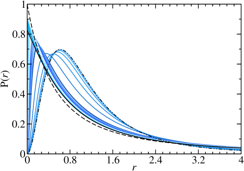
Figure A1: Examples for the Wigner-surmise like result (A76) for the ratio distribution of the eigenvalues of $\hat{H}^{0\to 0}$. With increasing $\lambda$ a transition from the result (A48) to (A86) takes place. The analytical results (A48), (A49) and (A76) are shown as black solid,dashed and dash-dotted lines, respectively.

A.3 Analytical results for long-range correlation functions for the transition from Poisson to GUE

In Ref. 73 an exact analytical expression was derived for $Y_{2}^{0\to 2}(r)$ based on the graded eigenvalue method,

$$Y_{2}^{0\to 2}(r) =\frac{1}{2(\pi r)^{2}}\left[1-e^{-2\frac{r^{2}}{\tilde{\alpha}^{2}}}\cos(2\pi r)\right]-\frac{1}{(\pi\tilde{\alpha})^{2}}+\frac{1}{\pi}\int_{0}^{\infty}\rho d\rho e^{-\frac{\rho^{2}}{2c}}\int_{0}^{\pi}d\phi\cos(\phi)\left[\mathrm{Re}(A)+\mathrm{Re}(B)\right]$$ (A87)

$$A =\frac{e^{i\phi}\left[1-\frac{\rho}{\kappa}\sin\phi\right]}{1+i\frac{\rho e^{i\phi}}{2\kappa}}\exp\left[-i\frac{\rho^{2}}{2c\kappa}\frac{1}{1-\frac{\rho}{\kappa}\sin\phi}\right],B=\frac{e^{-i\phi}\left[1+\frac{\rho}{\kappa}\sin\phi\right]}{1+i\frac{\rho e^{-i\phi}}{2\kappa}}\exp\left[-i\frac{\rho^{2}}{2c\kappa}\frac{1}{1+\frac{\rho}{\kappa}\sin\phi}\right],$$

$$\kappa =\frac{r}{\pi\tilde{\alpha}^{2}},\,c=\frac{1}{(\pi\tilde{\alpha})^{2}}.$$

The number variance is deduced from (A87) via the relation

$$\Sigma_{0\to 2}^{2}(L)=L-2\int_{0}^{L}(L-r)Y_{2}^{0\to 2}(r)dr\,.$$ (A88)

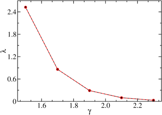
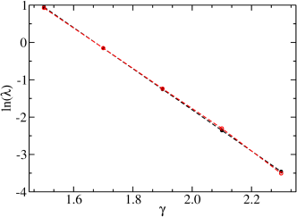
Figure A2: Left: Values of $\lambda$ obtained from the fit of the analytical result for $\Sigma^{2}(L)$ to the numerical results as function of $\gamma$. A fit of $\lambda\approx AN^{-B\gamma}$ yields $A=8034.46$ and $B=0.49$. Right: A linear fit $\ln(\lambda)\approx a-b\cdot\gamma\cdot{\rm ln}N$ yields $a=9.2122$ and $b=0.5$ (red).

In Ref. 48 an exact analytical result was obtained for the form factor,

$$K^{0\to 2}(\tilde{\tau})=1+\frac{2}{\xi}I_{1}(\xi)\exp{\left[-\pi\tilde{\alpha}^{2}\tilde{\tau}-\frac{\tilde{\alpha}^{2}\tilde{\tau}^{2}}{2}\right]}-\frac{\tilde{\tau}}{2\pi}\xi\int_{1}^{\infty}dt(t^{2}-1)I_{1}(\xi t)\exp\left[-t^{2}\frac{\tilde{\alpha}^{2}\tilde{\tau}^{2}}{2}-\pi\tilde{\alpha}^{2}\tilde{\tau}\right],$$

$$\xi=\sqrt{2\pi}\tilde{\alpha}^{2}\tilde{\tau}^{3/2},$$ (A89)

which was rederived in Ref. 44. For the evaluation of the integral for values of $\tau\gtrsim\tau_{min}$, with $\tau_{min}$ denoting the value of $\tau$ at the minimum of $K(\tau)$, we performed a transformation of the integration variable $t$ to $t=\sqrt{1+x}$ as in Ref. 44. We performed random-matrix simulations for values of $\gamma$ varying from $0.9\leq\gamma\leq 2.5$ in the RP model (1) and determined the corresponding values of $\lambda$ by fitting the analytical expression (A88) deduced from (A87) to the numerical ones. The resulting values are shown in Fig. A2. They agree well with those shown in Fig. 2 obtained from a fit of the distribution $P_{0\to 2}(s)$ given in (II.1) to the numerical results for the random-matrix obtained for the gRP model with $\beta=2$. A fit to $AN^{B\gamma}$ yields $B\simeq 0.5$ as expected from the definitions of the generalized and original RP model, Eqs. (2) with (3) and (1).

Appendix B Additional numerical results

In Fig. A3 we show the nearest-neighbor spacing distributions and its cumulative distribution for all values of $\gamma$ considered in this work. Figure A4 exhibits the energy-resolved average ratios $\langle r^{\rm min}\rangle$ as function of $\gamma$ and the center of the sliding energy interval which comprises 500 eigenvalues. In Fig. A4 are plotted the number variance and power spectrum for the same values of $\gamma$ as in Fig. A3. The asymptotic behavior of the latter is compared with approximate analytical results in terms of the spectral form factor in Fig. A6. In the intermediate region $1.3\lesssim\gamma\lesssim 1.8$ the approximation does not apply. In Fig. A7 the spectral form factor is depicted for six values of $\gamma$ for the GOE and the GUE. The turpuoise dashed lines show the analytical result for the corresponding WD ensemble.

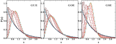
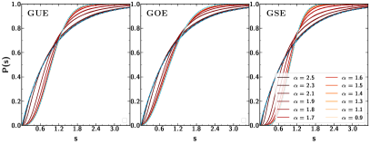
Figure A3: Left: Nearest-neighbor spacing distributions $P(s)$ obtained from random-matrix simulations for the gRP model for $\beta=2$ (left), $\beta=1$ (middle) and $\beta=4$ (right) for the values of $\gamma$ given in the insets of the right panel. The color changes from yellow to brown with increasing $\gamma$ and $P(s)$ experiences a transition from WD to Poisson statistics. Actually, for $\gamma=0.9$ the curves lie on top of the WD result (turquoise dashed line), and for $\gamma=2.5$ it is close to the result for Poissonian random numbers (turquoise dash-dot line). Right: Same as left for the cumulative nearest-neighbor spacing distribution.

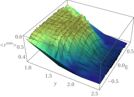
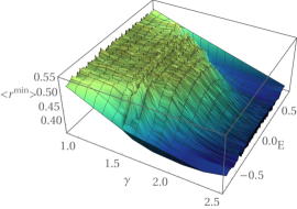
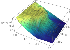
Figure A4: Average r-ratios $\langle r^{\rm min}\rangle$ as a function of $\alpha$ and energy center of a sliding window of 500 levels for N=65534. In the 3D plot Dark blue corresponds to the result for Poisson, yellow to that for GUE (left), GOE (middle) and GSE (right). Here, the eigenvalues were shifted such that the band center is at zero and then divided by their maximum value so that their values range from -1 to +1.

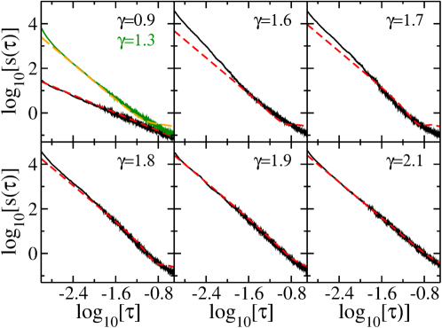
Figure A6: Comparison of the power spectrum for various values of $\gamma$ with an analytical approximation in terms of the spectral form factor (see main text). We find clear deviations in the range $1.3\lesssim\gamma\lesssim 1.8$ where the exponent $\mu$ shown in Fig. 8 exhibits a drastic change.

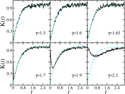
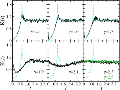
Figure A7: Left: Form factor obtained from the random-matrix simulations for the gRP Hamiltonian (2) (black) for the transition from Poisson to GOE for various values of $\gamma$. The turquoise line show the analytical curve for the GOE. Right: Form factor obtained from the random-matrix simulations for the gRP Hamiltonian (2) (black) for the transition from Poisson to GSE for various values of $\gamma$. The turquoise line shows the analytical curve for the GSE.

References

- Mehta [2004] M. L. Mehta, Random Matrices (Elsevier, Amsterdam, 2004).
- Porter [1965] C. E. Porter, Statistical Theories of Spectra: Fluctuations (Academic, New York, 1965).
- Brody et al. [1981] T. A. Brody, J. Flores, J. B. French, P. A. Mello, A. Pandey, and S. S. M. Wong, Random-matrix physics: spectrum and strength fluctuations, Rev. Mod. Phys. 53, 385 (1981).
- Haq et al. [1982] R. U. Haq, A. Pandey, and O. Bohigas, Fluctuation properties of nuclear energy levels: Do theory and experiment agree?, Phys. Rev. Lett. 48, 1086 (1982).
- Guhr and Weidenmüller [1989] T. Guhr and H. A. Weidenmüller, Coexistence of collectivity and chaos in nuclei, Ann. Phys. 193, 472 (1989).
- Guhr et al. [1998] T. Guhr, A. Müller-Groeling, and H. A. Weidenmüller, Random-matrix theories in quantum physics: common concepts, Phys. Rep. 299, 189 (1998).
- Weidenmüller and Mitchell [2009] H. Weidenmüller and G. Mitchell, Random matrices and chaos in nuclear physics: Nuclear structure, Rev. Mod. Phys. 81, 539 (2009).
- Mitchell et al. [2010] G. E. Mitchell, A. Richter, and H. A. Weidenmüller, Random matrices and chaos in nuclear physics: Nuclear reactions, Rev. Mod. Phys. 82, 2845 (2010).
- Gómez et al. [2011] J. Gómez, K. Kar, V. Kota, R. Molina, A. Relaño, and J. Retamosa, Many-body quantum chaos: Recent developments and applications to nuclei, Phys. Rep. 499, 103 (2011).
- Guhr [2009] T. Guhr, Doorway mechanism in many body systems and in quantum billiards, Acta Pol. A 116, 741 (2009).
- Enders et al. [2000] J. Enders, T. Guhr, N. Huxel, P. von Neumann-Cosel, C. Rangacharyulu, and A. Richter, Level spacing distribution of scissors mode states in heavy deformed nuclei, Phys. Lett. B 486, 273 (2000).
- Enders et al. [2004] J. Enders, T. Guhr, A. Heine, P. von Neumann Cosel, V. Ponomarev, A. Richter, and J. Wambach, Spectral statistics and the fine structure of the electric pygmy dipole resonance in n=82 nuclei, Nuclear Physics A 741, 3 (2004).
- Dietz et al. [2017] B. Dietz, A. Heusler, K. H. Maier, A. Richter, and B. A. Brown, Chaos and regularity in the doubly magic nucleus , Phys. Rev. Lett. 118, 012501 (2017).
- Dietz et al. [2018] B. Dietz, B. A. Brown, U. Gayer, N. Pietralla, V. Y. Ponomarev, A. Richter, P. C. Ries, and V. Werner, Chaos and regularity in the spectra of the low-lying dipole excitations of , Phys. Rev. C 98, 054314 (2018).
- Berry and Tabor [1977a] M. V. Berry and M. Tabor, Level clustering in the regular spectrum, Proc. R. Soc. London A 356, 375 (1977a).
- Casati et al. [1980] G. Casati, F. Valz-Gris, and I. Guarnieri, On the connection between quantization of nonintegrable systems and statistical theory of spectra, Lett. Nuovo Cimento 28, 279 (1980).
- Bohigas et al. [1984] O. Bohigas, M. J. Giannoni, and C. Schmit, Characterization of chaotic quantum spectra and universality of level fluctuation laws, Phys. Rev. Lett. 52, 1 (1984).
- Bohigas and Pato [2004] O. Bohigas and M. P. Pato, Missing levels in correlated spect, Phys. Lett. B 595, 171 (2004).
- Haake et al. [2018] F. Haake, S. Gnutzmann, and M. Kuś, Quantum Signatures of Chaos (Springer-Verlag, Heidelberg, 2018).
- Berry and Tabor [1977b] M. V. Berry and M. Tabor, Calculating the bound spectrum by path summation in actionangle variables, J. Phys. A 10, 371 (1977b).
- Scharf et al. [1988] R. Scharf, B. Dietz, M. Kuś, F. Haake, and M. V. Berry, Kramers’ degeneracy and quartic level repulsion, Europhys. Lett. 5, 383 (1988).
- Giannoni et al. [1989] M. Giannoni, A. Voros, and J. Zinn-Justin, eds., Chaos and Quantum Physics (Elsevier, Amsterdam, 1989).
- Stöckmann [2000] H.-J. Stöckmann, Quantum Chaos: An Introduction (Cambridge University Press, Cambridge, 2000).
- Stöckmann and Stein [1990] H.-J. Stöckmann and J. Stein, ”quantum” chaos in billiards studied by microwave absorption, Phys. Rev. Lett. 64, 2215 (1990).
- Sridhar [1991] S. Sridhar, Experimental observation of scarred eigenfunctions of chaotic microwave cavities, Phys. Rev. Lett. 67, 785 (1991).
- Gräf et al. [1992] H.-D. Gräf, H. L. Harney, H. Lengeler, C. H. Lewenkopf, C. Rangacharyulu, A. Richter, P. Schardt, and H. A. Weidenmüller, Distribution of eigenmodes in a superconducting stadium billiard with chaotic dynamics, Phys. Rev. Lett. 69, 1296 (1992).
- Deus et al. [1995] S. Deus, P. M. Koch, and L. Sirko, Statistical properties of the eigenfrequency distribution of three-dimensional microwave cavities, Phys. Rev. E 52, 1146 (1995).
- Hul et al. [2004] O. Hul, S. Bauch, P. Pakoński, N. Savytskyy, K. Życzkowski, and L. Sirko, Experimental simulation of quantum graphs by microwave networks, Phys. Rev. E 69, 056205 (2004).
- Allgaier et al. [2014] M. Allgaier, S. Gehler, S. Barkhofen, H.-J. Stöckmann, and U. Kuhl, Spectral properties of microwave graphs with local absorption, Phys. Rev. E 89, 022925 (2014).
- Białous et al. [2016] M. Białous, V. Yunko, S. Bauch, M. Ławniczak, B. Dietz, and L. Sirko, Power spectrum analysis and missing level statistics of microwave graphs with violated time reversal invariance, Phys. Rev. Lett. 117, 144101 (2016).
- Pandey and Shukla [1991] A. Pandey and P. Shukla, Eigenvalue correlations in the circular ensembles, J. Phys. A 24, 3907 (1991).
- Lenz [1992] G. Lenz, Zufallsmatrixtheorie und Nichtgleichgewichtsprozesse der Niveaudynamik, Ph.D. thesis, Fachbereich Physik der Universität-Gesamthochschule Essen (1992).
- Bohigas et al. [1995] O. Bohigas, M.-J. Giannoni, A. M. O. de Almeidaz, and C. Schmit, Chaotic dynamics and the goe-gue transition, Nonlinearity 8, 203 (1995).
- Guhr [1996a] T. Guhr, Ann. Phys. 250, 145 (1996a).
- French et al. [1985] J. B. French, V. K. B. Kota, A. Pandey, and S. Tomsovic, Bound on time-reversal noninvariance in the nuclear hamiltonian, Phys. Rev. Lett. 54, 2313 (1985).
- Pluhař et al. [1995] Z. Pluhař, H. A. Weidenmüller, J. Zuk, C. Lewenkopf, and F. Wegner, Crossover from orthogonal to unitary symmetry for ballistic electron transport in chaotic microstructures, Ann. Phys. 243, 1 (1995).
- Aßmann et al. [2016] M. Aßmann, J. Thewes, D. Fröhlich, and M. Bayer, Quantum chaos and breaking of all anti-unitary symmetries in Rydberg excitons, Nature Materials 15, 741 (2016).
- So et al. [1995] P. So, S. M. Anlage, E. Ott, and R. Oerter, Wave chaos experiments with and without time reversal symmetry: GUE and GOE statistics, Phys. Rev. Lett. 74, 2662 (1995).
- Stoffregen et al. [1995] U. Stoffregen, J. Stein, H.-J. Stöckmann, M. Kuś, and F. Haake, Microwave billiards with broken time reversal symmetry, Phys. Rev. Lett. 74, 2666 (1995).
- Wu et al. [1998] D. H. Wu, J. S. A. Bridgewater, A. Gokirmak, and S. M. Anlage, Probability amplitude fluctuations in experimental wave chaotic eigenmodes with and without time-reversal symmetry, Phys. Rev. Lett. 81, 2890 (1998).
- Dietz et al. [2019] B. Dietz, T. Klaus, M. Miski-Oglu, A. Richter, and M. Wunderle, Partial time-reversal invariance violation in a flat, superconducting microwave cavity with the shape of a chaotic Africa billiard, Phys. Rev. Lett. 123, 174101 (2019).
- Rosenzweig and Porter [1960] N. Rosenzweig and C. E. Porter, ”repulsion of energy levels” in complex atomic spectra, Phys. Rev. 120, 1698 (1960).
- Zhang et al. [2023] X. Zhang, W. Zhang, J. Che, and B. Dietz, Experimental test of the rosenzweig-porter model for the transition from poisson to gaussian unitary ensemble statistics, Phys. Rev. E 108, 044211 (2023).
- Kravtsov et al. [2015] V. E. Kravtsov, I. M. Khaymovich, E. Cuevas, and M. Amini, A random matrix model with localization and ergodic transitions, New J. Phys. 17, 122002 (2015).
- Brézin and Hikami [1996] E. Brézin and S. Hikami, Correlations of nearby levels induced by a random potential, Nucl. Phys. B 479, 697 (1996).
- Bogomolny and Sieber [2018a] E. Bogomolny and M. Sieber, Eigenfunction distribution for the rosenzweig-porter model, Phys. Rev. E 98, 032139 (2018a).
- Pandey [1995] A. Pandey, Brownian-motion model of discrete spectra, Chaos, Solitons & Fractals 5, 1275 (1995).
- Kunz and Shapiro [1998] H. Kunz and B. Shapiro, Transition from poisson to gaussian unitary statistics: The two-point correlation function, Phys. Rev. E 58, 400 (1998).
- von Soosten and Warzel [2018] P. von Soosten and S. Warzel, The phase transition in the ultrametric ensemble and local stability of Dyson Brownian motion, Electron. J. of Probab. 23, 1 (2018).
- Abanin et al. [2019] D. A. Abanin, E. Altman, I. Bloch, and M. Serbyn, Colloquium: Many-body localization, thermalization, and entanglement, Rev. Mod. Phys. 91, 021001 (2019).
- Alet and Laflorencie [2018] F. Alet and N. Laflorencie, Many-body localization: An introduction and selected topics, Comptes Rendus Physique 19, 498 (2018), quantum simulation / Simulation quantique.
- Sierant et al. [2024] P. Sierant, M. Lewenstein, A. Scardicchio, L. Vidmar, and J. Zakrzewski, Many-body localization in the age of classical computing (2024), arXiv:2403.07111 [cond-mat.dis-nn] .
- Landon et al. [2019] B. Landon, P. Sosoe, and H.-T. Yau, Fixed energy universality of dyson brownian motion, Advances in Mathematics 346, 1137 (2019).
- Facoetti et al. [2016] D. Facoetti, P. Vivo, and G. Biroli, From non-ergodic eigenvectors to local resolvent statistics and back: A random matrix perspective, Europhysics Letters 115, 47003 (2016).
- Truong and Ossipov [2016] K. Truong and A. Ossipov, Eigenvectors under a generic perturbation: Non-perturbative results from the random matrix approach, Europhysics Letters 116, 37002 (2016).
- Monthus [2017] C. Monthus, Multifractality of eigenstates in the delocalized non-ergodic phase of some random matrix models: Wigner–weisskopf approach, Journal of Physics A: Mathematical and Theoretical 50, 295101 (2017).
- von Soosten and Warzel [2019] P. von Soosten and S. Warzel, Non-ergodic delocalization in the rosenzweig–porter model, Letters in Mathematical Physics 109, 905 (2019).
- Pino et al. [2019] M. Pino, J. Tabanera, and P. Serna, From ergodic to non-ergodic chaos in rosenzweig–porter model, Journal of Physics A: Mathematical and Theoretical 52, 475101 (2019).
- Tomasi et al. [2019] G. D. Tomasi, M. Amini, S. Bera, I. M. Khaymovich, and V. E. Kravtsov, Survival probability in Generalized Rosenzweig-Porter random matrix ensemble, SciPost Phys. 6, 014 (2019).
- Berkovits [2020] R. Berkovits, Super-poissonian behavior of the rosenzweig-porter model in the nonergodic extended regime, Phys. Rev. B 102, 165140 (2020).
- Skvortsov et al. [2022] M. A. Skvortsov, M. Amini, and V. E. Kravtsov, Sensitivity of (multi)fractal eigenstates to a perturbation of the hamiltonian, Phys. Rev. B 106, 054208 (2022).
- Hopjan and Vidmar [2023] M. Hopjan and L. Vidmar, Scale-invariant critical dynamics at eigenstate transitions, Phys. Rev. Res. 5, 043301 (2023).
- Čadež et al. [2023] T. Čadež, B. Dietz, D. Rosa, A. Andreanov, K. Slevin, and T. Ohtsuki, Machine learning wave functions to identify fractal phases, Phys. Rev. B 108, 184202 (2023).
- Buijsman and Lev [2022] W. Buijsman and Y. B. Lev, Circular Rosenzweig-Porter random matrix ensemble, SciPost Phys. 12, 082 (2022).
- Buijsman [2024] W. Buijsman, Long-range spectral statistics of the rosenzweig-porter model, Phys. Rev. B 109, 024205 (2024).
- De Tomasi and Khaymovich [2022] G. De Tomasi and I. M. Khaymovich, Non-hermitian rosenzweig-porter random-matrix ensemble: Obstruction to the fractal phase, Phys. Rev. B 106, 094204 (2022).
- Khaymovich et al. [2020] I. M. Khaymovich, V. E. Kravtsov, B. L. Altshuler, and L. B. Ioffe, Fragile extended phases in the log-normal rosenzweig-porter model, Phys. Rev. Research 2, 043346 (2020).
- Kutlin and Khaymovich [2024] A. Kutlin and I. M. Khaymovich, Anatomy of the eigenstates distribution: A quest for a genuine multifractality, SciPost Phys. 16, 008 (2024).
- Sarkar et al. [2023] M. Sarkar, R. Ghosh, and I. M. Khaymovich, Tuning the phase diagram of a rosenzweig-porter model with fractal disorder, Phys. Rev. B 108, L060203 (2023).
- Bogomolny and Sieber [2018b] E. Bogomolny and M. Sieber, Power-law random banded matrices and ultrametric matrices: Eigenvector distribution in the intermediate regime, Phys. Rev. E 98, 042116 (2018b).
- Guhr [1996b] T. Guhr, Transition from poisson regularity to chaos in a time-reversal noninvariant system, Phys. Rev. Lett. 76, 2258 (1996b).
- Guhr [1996c] T. Guhr, Transitions toward quantum chaos: With supersymmetry from poisson to gauss, Ann. Phys. 250, 145 (1996c).
- Frahm et al. [1998] K. M. Frahm, T. Guhr, and A. Müller-Groeling, Between poisson and gue statistics: Role of the breit–wigner width, Ann. Phys. 270, 292 (1998).
- Lenz and Haake [1991] G. Lenz and F. Haake, Reliability of small matrices for large spectra with nonuniversal fluctuations, Phys. Rev. Lett. 67, 1 (1991).
- Pandey [1981] A. Pandey, Ann. Phys. 134, 110 (1981).
- Relaño et al. [2002] A. Relaño, J. M. G. Gómez, R. A. Molina, J. Retamosa, and E. Faleiro, Quantum chaos and noise, Phys. Rev. Lett. 89, 244102 (2002).
- Faleiro et al. [2004] E. Faleiro, J. M. G. Gómez, R. A. Molina, L. Muñoz, A. Relaño, and J. Retamosa, Theoretical derivation of noise in quantum chaos, Phys. Rev. Lett. 93, 244101 (2004).
- Haake et al. [1991] F. Haake, G. Lenz, P. Seba, J. Stein, H.-J. Stöckmann, and K. Życzkowski, Manifestation of wave chaos in pseudointegrable microwave resonators, Phys. Rev. A 44, R6161 (1991).
- Kota [2014] V. K. B. Kota, Embedded Random Matrix Ensembles in Quantum Physics (Springer-Verlag, Heidelberg, 2014).
- Bogomolny et al. [1999] E. B. Bogomolny, U. Gerland, and C. Schmit, Models of intermediate spectral statistics, Phys. Rev. E 59, R1315 (1999).
- Abramowitz and Stegun [2013] M. Abramowitz and I. A. Stegun, eds., Handbook of Mathematical Functions with Formulas, Graphs and Mathematical Tables (Dover, New York, 2013).
- Gradshteyn and Ryzhik [2007] I. S. Gradshteyn and I. M. Ryzhik, eds., Tables of Integrals, Series and Products (Elsevier, Amsterdam, 2007).
- Kota and Sumedha [1999] V. K. B. Kota and S. Sumedha, Transition curves for the variance of the nearest neighbor spacing distribution for poisson to gaussian orthogonal and unitary ensemble transitions, Phys. Rev. E 60, 3405 (1999).
- Schierenberg et al. [2012] S. Schierenberg, F. Bruckmann, and T. Wettig, Wigner surmise for mixed symmetry classes in random matrix theory, Phys. Rev. E 85, 061130 (2012).
- Dietz and Haake [1990] B. Dietz and F. Haake, Taylor and padé analysis of the level spacing distributions of random-matrix ensembles, Z. Phys. A 80, 153 (1990).
- Oganesyan and Huse [2007] V. Oganesyan and D. A. Huse, Localization of interacting fermions at high temperature, Phys. Rev. B 75, 155111 (2007).
- Atas et al. [2013a] Y. Y. Atas, E. Bogomolny, O. Giraud, and G. Roux, Distribution of the ratio of consecutive level spacings in random matrix ensembles, Phys. Rev. Lett. 110, 084101 (2013a).
- Atas et al. [2013b] Y. Atas, E. Bogomolny, O. Giraud, P. Vivo, and E. Vivo, Joint probability densities of level spacing ratios in random matrices, J. Phys. A 46, 355204 (2013b).
- Venturelli et al. [2023] D. Venturelli, L. F. Cugliandolo, G. Schehr, and M. Tarzia, Replica approach to the generalized Rosenzweig-Porter model, SciPost Phys. 14, 110 (2023).
- French et al. [1988] J. French, V. Kota, A. Pandey, and S. Tomsovic, Statistical properties of many-particle spectra vi. fluctuation bounds on n-nt-noninvariance, Ann. Phys. 181, 235 (1988).
- Leyvraz and Seligman [1990] F. Leyvraz and T. H. Seligman, Self-consistent perturbation theory for random matrix ensembles, J. Phys. A: Math. Gen. 23, 1555 (1990).
- Altland and Zirnbauer [1997] A. Altland and M. R. Zirnbauer, Nonstandard symmetry classes in mesoscopic normal-superconducting hybrid structures, Phys. Rev. B 55, 1142 (1997).
- Riser et al. [2017] R. Riser, V. A. Osipov, and E. Kanzieper, Power spectrum of long eigenlevel sequences in quantum chaotic systems, Phys. Rev. Lett. 118, 204101 (2017).
- Riser and Kanzieper [2023] R. Riser and E. Kanzieper, Power spectrum of the circular unitary ensemble, Physica D: Nonlinear Phenomena 444, 133599 (2023).
- Molina et al. [2007] R. Molina, J. Retamosa, L. Muñoz, A. Relaño, and E. Faleiro, Power spectrum of nuclear spectra with missing levels and mixed symmetries, Phys. Lett. B 644, 25 (2007).
- Che et al. [2021] J. Che, J. Lu, X. Zhang, B. Dietz, and G. Chai, Missing-level statistics in classically chaotic quantum systems with symplectic symmetry, Phys. Rev. E 103, 042212 (2021).
- Kullback and Leibler [1951] S. Kullback and R. A. Leibler, On Information and Sufficiency, The Annals of Mathematical Statistics 22, 79 (1951).
- Sels and Polkovnikov [2021] D. Sels and A. Polkovnikov, Dynamical obstruction to localization in a disordered spin chain, Phys. Rev. E 104, 054105 (2021).
- Slevin and Ohtsuki [2014] K. Slevin and T. Ohtsuki, Critical exponent for the anderson transition in the three-dimensional orthogonal universality class, New Journal of Physics 16, 10.1088/1367-2630/16/1/015012 (2014).
- Press et al. [2002] W. H. Press, S. A. Teukolsky, W. T. Vetterling, and B. P. Flannery, Numerical recipes in C: the art of scientific computing, 2nd Edition (Cambridge University Press, 2002).
- Rodriguez et al. [2010] A. Rodriguez, L. J. Vasquez, K. Slevin, and R. A. Römer, Critical parameters from a generalized multifractal analysis at the anderson transition, Phys. Rev. Lett. 105, 046403 (2010).
- Rodriguez et al. [2011] A. Rodriguez, L. J. Vasquez, K. Slevin, and R. A. Römer, Multifractal finite-size scaling and universality at the anderson transition, Phys. Rev. B 84, 134209 (2011).
- Pandey et al. [2020] M. Pandey, P. W. Claeys, D. K. Campbell, A. Polkovnikov, and D. Sels, Adiabatic eigenstate deformations as a sensitive probe for quantum chaos, Phys. Rev. X 10, 041017 (2020).
- Pechukas [1983] P. Pechukas, Distribution of energy eigenvalues in the irregular spectrum, Phys. Rev. Lett. 51, 943 (1983).
- Sierant et al. [2019] P. Sierant, A. Maksymov, M. Kuś, and J. Zakrzewski, Fidelity susceptibility in gaussian random ensembles, Phys. Rev. E 99, 050102 (2019).
- Nandy et al. [2022] D. K. Nandy, T. Čadež, B. Dietz, A. Andreanov, and D. Rosa, Delayed thermalization in the mass-deformed sachdev-ye-kitaev model, Phys. Rev. B 106, 245147 (2022).
- Orlov et al. [2023] P. Orlov, A. Tiutiakina, R. Sharipov, E. Petrova, V. Gritsev, and D. V. Kurlov, Adiabatic eigenstate deformations and weak integrability breaking of heisenberg chain, Phys. Rev. B 107, 184312 (2023).
- Harish-Chandra [1958] Harish-Chandra, Spherical functions on a semisimple lie group, i, Am. J. Math. 80, https://doi.org/10.2307/2372786 (1958).
- Pandey and Mehta [1983] A. Pandey and M. L. Mehta, Gaussian ensembles of random hermitian matrices intermediate between orthogonal and unitary ones, Commun. Math. Phys. 87, 449 (1983).