Causality for Earth Science - A Review on Time-series and Spatiotemporal Causality Methods
Abstract
This survey paper covers the breadth and depth of time-series and spatiotemporal causality methods, and their applications in Earth Science. More specifically, the paper presents an overview of causal discovery and causal inference, explains the underlying causal assumptions, and enlists evaluation techniques and key terminologies of the domain area. The paper elicits the various state-of-the-art methods introduced for time-series and spatiotemporal causal analysis along with their strengths and limitations. The paper further describes the existing applications of several methods for answering specific Earth Science questions such as extreme weather events, sea level rise, teleconnections etc. This survey paper can serve as a primer for Data Science researchers interested in data-driven causal study as we share a list of resources, such as Earth Science datasets (synthetic, simulated and observational data) and open source tools for causal analysis. It will equally benefit the Earth Science community interested in taking an AI-driven approach to study the causality of different dynamic and thermodynamic processes as we present the open challenges and opportunities in performing causality-based Earth Science study.
Significance Statement
Causality is the study of discovering cause-effect relations in data. Earth Science can benefit greatly from causal methods as researchers have started utilizing causality to understand the complex interactions leading to climate change, long term weather patterns, extreme weather events, etc. This paper provides a primer to causal inference and causal discovery for different Earth Science domains with some of the existing applications and open questions for future research. The paper also comprises a holistic list of available tools and datasets that can help both Data Science and Earth Science communities in performing causal analysis on Earth data.
1 Introduction
Earth science is the study of the Earth’s physical properties, structure, and processes. It encompasses a wide range of topics including geology, meteorology, oceanography, and environmental science (Smith and Pun, 2013). Earth science research relies purely on climate models that replicate complex dynamical systems. Climate models allow scientists to better understand how the Earth’s climate system works and how it might change in the future. These models can be used to make predictions about future climate change and to test different scenarios, for instance studying the global carbon footprint to reduce greenhouse gas emissions. However, climate models are computationally expensive and require a lot of computing power to run. This is because they need to simulate many different dynamic processes that occur in the atmosphere, oceans, and on land. For instance a simulation that works on cloud formation or generating ocean currents.
In recent decades, there has been a significant increase in the availability of large-scale climate data from various observational sources (such as satellite remote sensing, station-based or field site measurements) and Earth system model outputs (Guo et al., 2015). This data, along with the increasing computational power, has opened up new ways to use data-driven methods for observational causal discoveries without relying on the correlation and trend analyses of the data (Rubin, 2005). In Earth system sciences, causal structure discovery (CSD) models are making inroads into several domains (Melkas et al., 2021). Climate causal studies pose the changing trend of applying the current state-of-the-art climate data not only to correlation and regression methods but also to causal inference methods. For instance, climate researchers have realized that climate simulations introduce ambiguous values to the datasets which makes them not applicable in decision-making applications (Ebert-Uphoff and Deng, 2012). After understanding the importance of data-driven methods in climate science, scientists have started to explore different causal structure algorithms and Bayesian networks to get deeper insights into causal hypotheses and the evaluation of physical models (Ebert-Uphoff and Deng, 2012). In the past, Bayesian models were used to compute the probability of climate data where it is needed for forecasting and risk assessment tools. Now, Bayesian models are significantly used in climate science to test the causal hypothesis to develop decision-making algorithms. A recent research study (Nowack et al., 2020) evaluated the ability of the Coupled Model Intercomparison Project Phase 5 (CMIP5) to simulate atmospheric dynamical interactions using the causal model evaluation (CME) framework. This study highlighted the potential of the CME framework to offer a pathway to reducing uncertainties in climate change projections by quantifying differences between models and observations. To sum it up, causality methods can play a crucial role in Earth Science studies by helping researchers understand and quantify the cause-and-effect relationships within complex Earth systems for a variety of usecases. Some of these include: identifying the primary drivers of environmental changes, attributing specific climate events like volcanic eruptions, identifying causes of extreme weather events such as hurricanes, droughts and floods, helping in the prediction of natural hazards such as earthquakes and tsunamis, designing effective pollution control policies, understanding El Niño/La Niña events and their global climate impacts, etc.
This survey paper is therefore an effort to provide an overview of the current state of knowledge on causality in Earth Science. It will serve as a primer to help understand key concepts in causality and methods that are commonly used. In addition to existing survey papers (Table 1), our survey paper will help identify gaps in current causality-based Earth Science research and highlight areas where causal methods could be used to improve our understanding of the Earth’s system. The paper is organized as follows. Section 2 enlists some open challenges in causality-based study of Earth Science problems. Section 3 explains the concept of causal structure learning or ”Causal Discovery”. Here, we first explain the foundational concepts of causal discovery such as key terms, causal assumptions and the relevant evaluation metrics for the structure learning task. We then enlist several approaches to perform causal discovery on time-series and spatiotemporal data. Finally, we share the applications of causal discovery in Earth Science as found in the literature. Section 4 explains the process of estimating causal effects, also known as ”Causal Inference”. Just like the previous section, we first explain the key terms, causal assumption and evaluation metrics related to Causal inference. The subsequent topics elicits the various state-of-the-art methods introduced for time-series and spatiotemporal causal inference along with their strengths and limitations. This section further describes the existing applications of several causal inference methods for answering specific Earth Science questions such as extreme weather events, sea level rise, etc. In Section 5, we share a list of resources including Earth Science datasets (synthetic, simulated and observational data) and open source toolboxes for causal analysis. Lastly, we conclude our work and share potential research pathways in Section 6. We hope our paper equally benefits both the Data Science community interested in data-driven causal study and the Earth Science community interested in taking an AI-driven approach to study the causality of different dynamic and thermodynamic processes.
| Paper Title | Discovery | Inference | Datasets | Metrics | Software | Time series | Spatial |
|---|---|---|---|---|---|---|---|
| Inferring causation from time series in Earth system sciences (Runge et al., 2019b) | \xmark | \xmark | \xmark | \xmark | |||
| D’ya Like DAGs? A Survey on Structure Learning and Causal Discovery (Vowels et al., 2022) | \xmark | \xmark | |||||
| Survey and Evaluation of Causal Discovery Methods for Time Series (Assaad et al., 2022) | \xmark | \xmark | \xmark | ||||
| Causal Structure Learning (Heinze-Deml et al., 2018) | \xmark | \xmark | \xmark | \xmark | |||
| Review of Causal Discovery Methods Based on Graphical Models (Glymour et al., 2019) | \xmark | \xmark | \xmark | \xmark | \xmark | ||
| A Survey of Learning Causality with Data: Problems and Methods (Guo et al., 2020) | \xmark | ||||||
| Causal inference for time series analysis: problems,methods and evaluation (Moraffah et al., 2021) | \xmark | \xmark | |||||
| A Survey on Causal Discovery Methods for I.I.D. and Time Series Data (Hasan et al., 2023) | \xmark | \xmark | |||||
| Causal Inference for Time Series (Runge et al., 2023) | \xmark | \xmark | |||||
| A Primer on Deep Learning for Causal Inference (Koch et al., 2021) | \xmark | \xmark | \xmark | ||||
| Causal Discovery from Temporal Data: An Overview and New Perspectives (Gong et al., 2023) | \xmark | \xmark | \xmark | ||||
| A Survey on Causal Inference (Yao et al., 2021) | \xmark | \xmark | \xmark | \xmark | |||
| Causal inference for process understanding in Earth sciences (Massmann et al., 2021) | \xmark | \xmark | \xmark | \xmark | \xmark | ||
| Spatial Causality: A Systematic Review on Spatial Causal Inference (Akbari et al., 2023) | \xmark | \xmark | \xmark | \xmark | |||
| A review of spatial causal inference methods for environmental and epidemiological applications (Reich et al., 2021) | \xmark | \xmark | \xmark | ||||
| Our Survey |
| Earth Science Domain | Key Questions |
|---|---|
| Atmosphere | How do natural and anthropogenic activities influence greenhouse gas concentrations and atmospheric composition? |
| How do aerosols influence cloud formation, precipitation patterns, and regional climate variability? | |
| How are climate change and global warming influencing patterns of weather extremes, including heatwaves, | |
| droughts, extreme rainfall events, and storms? | |
| What are the mechanisms driving changes in atmospheric circulation patterns, such as shifts in jet streams | |
| and tropical cyclones? | |
| Cryosphere | What are the primary drivers of amplified Arctic warming and accelerated loss of sea ice? |
| How does Arctic amplification contribute to more frequent extreme heat, wildfire and increasing precipitation | |
| at high latitudes? | |
| What factors drive the loss of glacier mass in both the Arctic and Antarctic regions, and what implications does | |
| this have for global weather patterns? | |
| Hydrosphere | What are the climatic and non-climatic drives for water cycle change? |
| How does sea level rise impact water-related extreme events (e.g., floods and droughts)? | |
| What are the effects of alterations in soil moisture on local weather patterns, water security, and agricultural systems? | |
| Ocean | How are rising global temperatures affecting ocean temperatures, both at the surface and in deeper layers? |
| How is increased atmospheric carbon dioxide leading to ocean acidification? | |
| How is climate change affecting ocean circulation patterns, including the Gulf Stream and the Atlantic | |
| Meridional Overturning Circulation (AMOC)? | |
| What are the feedback loops between changes in the ocean carbon cycle and global climate dynamics? | |
| Biosphere | How is rising global temperature influencing the geographic ranges and habitats of species? |
| How does amplified Arctic warming affect polar biodiversity? | |
| What are the consequences of coral reef degradation? |
| Area | Challenges | Opportunities |
|---|---|---|
| Causal Discovery | Accurate modeling of complex processes that | Domain Knowledge based Causal Discovery |
| occur in the Earth’s system | ||
| Causal Discovery | Lack of ground truth information for validation | Synthetic datasets simulating Earth Science data |
| of causal models | distributions | |
| Causal Discovery | No information on true causal frequency | Multi-scale causal discovery |
| Causal Discovery / Causal Inference | Tackling biases in simulated data | Adjusting for hidden confounders |
| Causal Discovery / Causal Inference | High dimensional data | Extracting causally relevant variables, |
| Causal representation learning, Causal discovery | ||
| in low dimensional space | ||
| Causal Discovery / Causal Inference | Non-linear data distributions | Deep learning based Causal Discovery / |
| Inference methods | ||
| Causal Discovery | Seasonality / Non-stationarity in data | Incorporating periodicity / segmentation, |
| Sliding window analysis | ||
| Causal Inference | Tackling bias due to time-variying confounding | Matching Methods Treatment weighting methods |
| Causal Inference | Tackling bias due to spatial confounding | Neighboringhood weighting, Adjusting |
| spillover effects |
2 Open Challenges in Causality-based Earth Science Study
Due to the multi-way interactions between the atmosphere, hydrosphere, cryosphere, geosphere, and biosphere, studying causality between them is a challenging but important task, which makes it an area of high interest within the Earth Science community. Here, we have identified several fundamental questions within the Earth Science domain, particularly concerning the rapidly increasing emissions of greenhouse gases and the consequential impacts of climate change, which may benefit from causality methods. These inquiries pose significant challenges due to several factors: 1) Data availability may be inadequate or insufficient, hindering comprehensive analysis. 2) Climate data is inherently complex, with multiple dimensions, making analysis and interpretation challenging. 3) The complex interaction among numerous variables complicates the disentanglement of causal relationships and feedback mechanisms. 4) Confounding effects further hinder the clarification of causality. 5) The inability to conduct controlled laboratory experiments in climate science limits our understanding of causal relationships. 6) The current state of climate models may lack the sophistication and precision necessary to accurately capture the complex interactions among variables. In Table 2, we enlist some of the causality-related open questions in different Earth Science domains (Masson-Delmotte et al., 2021; Pörtner et al., 2022). In Table 3, we identify some of the challenges in performing observational causal discovery and causal inference in various domains of Earth Science and the opportunities they pave for researchers.
3 Causal Discovery
Causal discovery refers to the process of discovering causal relations and uncovering underlying data generation process in real world data, helping researchers make more informed decisions, predict outcomes, and understand how changes in one variable, state or process may lead to changes in others (Pearl, 1988). In recent years, several graph-based algorithms are proposed for discovering the causal structures from empirical data (Spirtes et al., 2000; Tian and Pearl, 2013). The important causal connections are discovered purely based on the statistical analyses of observation data. This section presents an overview of time-series and spatiotemporal causal discovery, the key concepts in causality, and common approaches for performing causal structure learning for both temporal and spatial datasets. It further includes brief overview of renowned causal discovery methods, their limitations and applications in Earth Science study. To begin with, we have enlisted the key terminologies in causal discovery in Table 7.
| Terminology | Explanation |
|---|---|
| Causal discovery models | It aims to discover causal structures from data |
| Causal inference | Estimating the strength of the causal relationship between two variables |
| Undirected Graph | A graph with no direction between the nodes |
| Probabilistic Graphical Model | It captures conditional independence relationships between interacting random variables. |
| Bayesian Network Model | A probabilistic graphical model that represents the conditional dependencies of a set of |
| random variables via a directed acyclic graph (DAG) | |
| Latent parameter | Unknown / hidden parameters or hypotheses |
| Conditional independence | Nodes that are not causally related / connected |
| Conditional dependence | Nodes that are causally related / connected |
| Markov Network | An undirected graphical model with a set of random variables having a Markov property |
| Correlation graph | It determines the correlation patterns in the data |
| Structural Causal Model | It provides a mathematical and graphical representation of causal relationships |
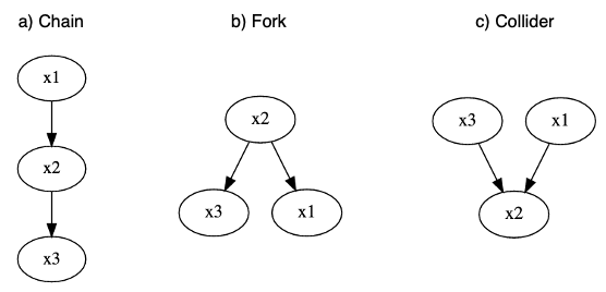
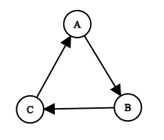
| Chain | Series-like structure (Figure 1: X1 causes X2 and X2 causes X3) |
| Fork | This structure shows a common cause of two effects. (Figure 1: X2 causes X1 and X3) |
| Collider | This structure include two causes of a single effect. (Figure 1: both X1 and X3 are the causes of X2) |
| Partial correlation | Partial correlation refers to lagging each of several variables on all relevant delays relative to another variable |
| Mutual independence | Each event is independent of any combination of other events in the collection |
| Structure learning | The process of inferring the structure of directed acyclic graph (DAG) from data |
| Moralization | Cognitive enhancement in causal selection process |
| Markov equivalence class | A set of DAGs that shares the same set of conditional independencies |
| Mutual Information Network | A measure of mutual information between two variables in the Bayesian network |
| Probability | Likelihood occurrence of an event |
3.1 Causal Assumptions
There are certain foundational principles and conditions, referred to as causal assumptions, that underlie the process of inferring causal relationships between variables. Different causal discovery methods may have different sets of assumptions. Some of the common causal assumptions are given below:
Causal Sufficiency:
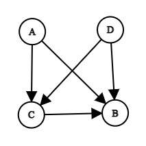
If for every measured variable in the data, all of its common causes are also measured, then the causal sufficiency assumption holds. As per this condition, a pair of variables is causally sufficient if all the common causes are measured, i.e. there are no latent confounders (Nogueira et al., 2021). Causal sufficiency is a very strong assumption as there is no such thing as a closed world. In real-world settings, it is not always the case that all possible causes are measured and hence, this assumption is often violated (Pellet and Elisseeff, 2008). Causal insufficiency occurs when for a set of variables V, there exists variables not present in V that are direct causes of more than one variable in V. In Figure 2, the variables are causally insufficient since another variable D outside of set V is the common cause of B & C.
Causal Markov Condition (CMC) / Causal Markov property:
The causal Markov assumption states that every node in a causal DAG G is independent of its non-descendants when conditioned on its parents. The idea behind the CMC is that when a variable’s effects (descendents) are ignored, all the relevant probabilistic information about that variable can be obtained from its direct causes (parents) (Scheines, 1997). CMC can also be explained in terms of d-separation. In a causal DAG G, all variables that are d-separated will be conditionally independent of each other in the respective probability distribution (Weinberger, 2018). This also implies that, among three disjoint nodes, one node must block all paths between the other two nodes (Nogueira et al., 2021). The causal Markov assumption is true in a DAG which is causally sufficient i.e. have no latent confounders.
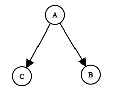
The CMC for the variables in the causal graph of Figure 3 is as follows:
C B A (C is independent of its non-descendant B conditioned on its parent A)
B C A (B is independent of its non-descendant C conditioned on its parent A)
Causal Faithfulness Condition (CFC):
The causal faithfulness assumption can be stated as follows. In a causal DAG G, no conditional independence between the variables holds unless entailed by the causal Markov condition (CMC). That is, CFC specifies which variables in a DAG will be probabilistically dependent (Weinberger, 2018). This is the converse of the Markov condition since CMC specifies which variables will be conditionally independent given their parents. With respect to d-separation, CFC means that except for the d-separated variables in a DAG, all other variables are dependent. In Figure 3, variables (A,C) and (A,B) are dependent. Based on CFC, it can be interpreted that no observed interdependency in the data is accidental, but results from the underlying causal mechanism (Druzdzel, 2009).
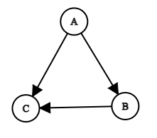
Acyclicity:
The acyclicity assumption states that no feedback loops are allowed in a causal graph. That is, there can be no directed paths from a variable back to itself similar to the structure of a directed acyclic graph (DAG). This is a very basic property of a causal graph Figure 4b) that must be fulfilled to represent the causal relationships accurately. Therefore, a causal graph is a DAG where no variable is its ancestor or its descendant (Greenland and Pearl, 2007).
(a) (b)
Data Assumptions:
Causal discovery approaches heavily rely on the available data and their assumptions. The data for performing any causal analysis can be either observational or interventional in nature, or both. To conduct causal discovery, often different types of assumptions about the data distribution are considered. They include data being linear or nonlinear, continuously valued or discrete valued, stationary or non-stationary (for temporal data), etc. Often assumptions about the varied noise distributions such as Gaussian, Gumbel, or Exponential noise to which the data may belong are made. Apart from these, some common assumptions about data are the existence of any sampling or selection bias, missing data, latent variables or noise, etc.
3.2 Evaluation Metrics
Evaluating the performance of causal discovery methods is crucial to assess their accuracy and reliability in identifying causal relationships from observational data. Given below are the commonly used evaluation metrics for causal discovery:
True Positive Rate (TPR):
TPR is the probability that an actual positive will test positive. Assuming the threshold of probability of an edge ranges from , TPR is defined as
| (1) |
where is the set of ground truth edges (i.e., .
False Positive Rate:
False positive rate (FPR) is the probability that an actual negative will test positive. Assuming the threshold of probability of an edge ranges from , is defined as
| (2) |
where is the set of ground truth missing edges (i.e., ).
Structural Hamming Distance (SHD):
Structural Hamming Distance (SHD) is the number of operators required to make two PDAGs match. The operators include adding or removing an undirected edge, and adding, removing or reversing the orientation of an edge. Let be the space of PDAGs over variables. SHD is defined as:
| (3) |
Structural Intervention Distance (SID):
Structural intervention distance (SID) is the number of vertice pairs for which the estimate DAG correctly predicts intervention distributions within the class of distributions that is Markov with respect to another DAG.
Area Over Curve (AOC):
Area over curve (AOC) simply area under curve (AUC) with . The curve is plotted with against as , where .
3.3 Common Approaches
Causal discovery methods can be categorized into following three major categories or approaches:
Constraint based Approach:
One of the most common approaches for performing causal discovery is the constraint-based approach which relies on testing the conditional independencies between the variables to identify the causal edges. In the constraint-based category, one of the oldest approaches is the Peter-Clark (PC) algorithm proposed by (Spirtes et al., 2000). It assumes faithfulness which implies that all the interdependencies in a DAG need to be under the d-separation criterion. Another well-known constraint-based approach is the Fast Causal Inference (FCI) algorithm (Spirtes et al., 2000) which differs from the PC algorithm as it violates causal sufficiency. That is, FCI assumes that some common causes may be unmeasured in real-world data.
Score based Approach:
The score-based approach is another common approach for causal discovery. Score-based approaches try to find the DAG with the maximum likelihood given the data (Triantafillou and Tsamardinos, 2016). They search over the space of all possible DAGs aiming to maximize a score function that depicts how well the graph fits the data. As a score function, the Bayesian Information Criterion (BIC) and other similar approaches are used to score the produced graphs and output the DAG with the best score (fits data the best). The score function can be modified to optimize or reduce the search space of all possible DAGs. In terms of performance, score-based algorithms can be cost ineffective as they need to score every possible DAG (Nogueira et al., 2021). When the number of variables increases even slightly, the number of possible graphs can grow super-exponentially. One of the famous score-based methods is the Greedy Equivalence Search (GES) algorithm (Chickering, 2002) that initially starts with an empty graph, and keeps on adding currently needed edges, and then deletes unnecessary edges as per the score function.
Functional Causal Models-based Approach:
Functional Causal Model (FCM) or also called SCM based approaches express the causal relationships in a specific functional form (a set of equations) where the variables are a function () of their direct causes (causal parents) and an independent noise term . These approaches rely heavily on the independent noise for the recovery and estimation of the causal relations. The FCM-based methods try to distinguish different DAGs in the same equivalence class by imposing additional assumptions on the data distributions and/or function classes. A wide range of FCM-based approaches exists for both temporal and non-temporal data that tries to handle both linear and non-linear causal relations using methods such as independent component analysis (ICA) (Stone, 2004) and additive noise models (ANMs) (Hoyer et al., 2008) respectively.
3.4 Time-Series Causal Discovery
Timeseries causal discovery refers to the process of identifying causal relationships between variables in a timeseries data setting. Causal discovery in timeseries data involves dealing with the specific challenges of temporal dependencies and potential feedback loops. It has been widely used in econometrics, neuroscience, and climate science (Spirtes et al., 2000; Zhou et al., 2014; Van Nes et al., 2015; Ghysels et al., 2016). Identifying time lags is an important aspect of causal discovery in timeseries data. It involves determining the delay or time difference between the cause and its effect. Time lags are crucial for understanding the dynamics of the causal relationship and for making accurate predictions in timeseries forecasting tasks. To identify time lags in causal relationships, researchers may use methods like cross-correlation analysis, autocorrelation, or timeseries cross-validation techniques (Spirtes et al., 2000). These methods help measure the strength of the association between variables at different time lags and assist in determining the optimal lag that maximizes the predictive performance or the strength of the causal relationship. We explain some of the widely used causal discovery methods below, along with their variants, underlying causal assumptions and limitations. A tabulated summary of these time-series causal discovery methods is given in Table 5.
| Method | Assumptions | Causal Relationship | Produced Edge | |||||
|---|---|---|---|---|---|---|---|---|
| Faithfulness | Sufficiency |
|
Linear | Non-linear | Instantaneous | Lagged | ||
| Granger Causality | \xmark | \xmark | \xmark | \xmark | \xmark | |||
| PCMCI | \xmark | |||||||
| PCMCI+ | ||||||||
| LPCMCI | \xmark | |||||||
| LiNGAM | \xmark | \xmark | \xmark | \xmark | \xmark | |||
| VarLiNGAM | \xmark | \xmark | \xmark | |||||
| TS-LiNGAM | \xmark | \xmark | \xmark | \xmark | \xmark | \xmark | ||
| TiMINo | \xmark | \xmark | \xmark | \xmark | \xmark | \xmark | ||
| NAVAR | \xmark | \xmark | \xmark | \xmark | \xmark | |||
3.4.1 Granger Causality, V-Granger
Granger causality is a statistical hypothesis test used to determine whether one time series can predict another Granger (1969). It is named after Clive Granger, a Nobel laureate economist who developed the concept. Granger causality is widely used in time series analysis to investigate the causal relationships between variables. The basic idea behind Granger causality is that if a time series X ”Granger-causes” another time series Y, then past values of X contain information that helps predict future values of Y beyond what can be predicted using past values of Y alone. It is important to note that Granger causality does not establish a true cause-and-effect relationship in the sense of a controlled experiment. It only identifies whether one time series provides useful predictive information for another time series. Nevertheless, Granger causality is commonly used in various fields, including economics, finance, engineering, and neuroscience, to explore relationships between time-varying data. However, it has limitations and assumptions. For instance, the choice of time lags can influence the results. GC assumes causal sufficiency condition, stationary and linear relationship and does not predict the direction of causal relation. The method is data hungry and requires sufficiently large sample size. Granger causality can be a useful exploratory tool, and its results should be interpreted carefully in the context of the specific data and research question at hand.
With the Granger Causality widely used in various fields to understand the causal relationship between time series, the presence of unobserved confounders poses a fundamental problem in observational studies, especially for non-linear Granger causality. V-Granger (Meng, 2019), overcomes the causal sufficiency limitation by estimating Granger causality in the presence of unobserved confounders using a variational autoencoder (VAE) to estimate the intractable posterior distribution and a recurrent neural network to model the temporal relationship in the data. Through experiments on synthetic and semi-synthetic datasets, as well as two real datasets: Butter and Temperature, the authors demonstrated how V-Granger outperforms the traditional Granger test in some cases. However, the method is not suitable for datasets with high noise levels.
3.4.2 PCMCI, PCMCI+, LPCMCI
PCMCI1 (Runge et al., 2019a) is a method for efficient estimation of causal graphs from high-dimensional time series datasets, which can be used for robust forecasting and the estimation and prediction of direct, total, and mediated effects. A baseline of PCMCI was first introduced by (Runge et al., 2015) for identifying causal gateways and mediators in complex spatiotemporal systems. The method combines the PC stable causal discovery algorithm with momentary conditional independence (MCI) to estimate causal networks from large-scale time series datasets in a two-step approach. The first step is to find lagged parents of all individual nodes using the PC stable method. The second step is to test the momentary conditional independence. As a result of the second step, if two nodes are independent, then there exists no cause-effect relationship between them. The outcome of this two-step method includes a causal adjacency matrix, corresponding lag values and strength of identified relationships given by p-values. PCMCI supports multiple linear and non-parametric conditional independence tests depending on the data distribution. For instance, the partial correlation or test assumes linear dependencies and Gaussian noise in the data. There are multiple variants of PCMCI available for different downstream tasks. For instance, PCMCI+ can be used for discovering contemporaneous and lagged causal relations in autocorrelated nonlinear time series datasets. For details on PCMCI’s implementation, independence tests available and different variants of PCMCI, please refer to their Github111https://github.com/jakobrunge/tigramite repository.
Similarly, Latent PCMCI or LPCMCI1 (Gerhardus and Runge, 2020) is a constraint-based approach which is a variant of the PCMCI algorithm for causal discovery from large-scale time series data in the presence of hidden confounders. This method is specialized to learn lag-specific causal relationships for linear and nonlinear, lagged and contemporaneous causal discovery from observational time series data.
3.4.3 LinGAM, VARLiNGAM, TS-LiNGAM
LinGAM222https://lingam.readthedocs.io/en/latest/index.html (Linear Non-Gaussian Acyclic Model) (Shimizu et al., 2006) is a framework used for causal discovery and estimation of causal effects from observational data. It focuses on identifying linear causal relationships among variables while considering non-Gaussian noise distributions. LinGAM assumes acyclic causal relationships among variables, meaning it aims to identify a directed acyclic graph (DAG) that represents the underlying causal structure. VARLiNGAM Hyvärinen et al. (2010) extends the foundational LiNGAM model to encompass scenarios involving time series. This augmentation involves integrating the core LiNGAM model with the conventional vector autoregressive models (VAR). Consequently, it facilitates the exploration of causal relationships encompassing both delayed and concurrent (instantaneous) effects. This stands in contrast to the traditional VAR framework, which solely examines causal relations with a time delay. VARLiNGAM holds similar causal assumptions as the base LinGAM model, such as, data linearity, causal sufficiency with no hidden confounders, acyclicity of contemporaneous causal relations and non-gaussian continuous error variables.
TS-LiNGAM (Hyvärinen et al., 2008) is a generalization of the LiNGAM algorithm which uses a non-Gaussianity assumption to estimate both instantaneous and lagged causal edges. The model is a combination of autoregressive models and structural equation modeling (SEM). It assumes the external noises to be mutually independent, temporally uncorrelated, and to be non-Gaussian. TS-LiNGAM combines classic least-squares estimation of an autoregressive (AR) model with LiNGAM estimation. It does so in four steps: i) Estimation of a classic autoregressive model, ii) Residuals computation, iii) Performing LiNGAM analysis on the residuals, and iv) Computation of the causal effect estimates. The method has been evaluated on real datasets such as financial (stock) data and magnetoencephalographic data i.e measurements of the electric activity in the brain.
3.4.4 TiMiNo
TiMINo (Peters et al., 2013) approach provides a new method at that time for causal inference on time series data that overcomes some of the methodological issues of previous methods that could not capture nonlinear and instantaneous effects. Specifically, TiMINo extends Structural Equation Models (SEMs) to the time series setting, and uses a restricted function class to provide general identifiability results including lagged and instantaneous effects that can be nonlinear and unfaithful, and non-instantaneous feedback between the time series. Given a sample of finite and continuous-distributed multivariate time series data, and output the summary time graph if the input data satisfies model assumptions. Otherwise, if the input fails the assumptions, TiMINo causality remains mostly undecided instead of drawing wrong causal conclusions. The model is defined as , where is the time lag for independence test, is the set of parent nodes of node , is a time-series data with finite and continuous distribution, and is a noise vector jointly independent over i and t. The approach assumes that each time series is a function of all direct causes and some noise variable, and restricts the function class to provide general identifiability results. Potential weaknesses of TiMINo are discussed including the possibility of fitting a model in the wrong direction and the effects of independence testing on smaller datasets.
3.4.5 Tidybench algorithms
(Weichwald et al., 2020) presents four algorithms333https://github.com/sweichwald/tidybench for causal discovery from time series data to address some common challenges such as time-aggregation, time-delays, and time-subsampling. The algorithms also focus on the properties of realistic weather and climate data and were among the winning algorithms in the Causality 4 Climate (C4C) competition at the NeurIPS 2019 conference. The output from these algorithms is an edge score matrix that contains a score for each pair of variables (, ) which represents the likelihood that the edge → exists. The algorithms are based on the following concept. Present values are regressed on past values and the regression coefficients are inspected to decide if one variable is a Granger-cause of another. Following is a brief description of all the algorithms: (i) SLARAC (Subsampled Linear Auto-Regression Absolute Coefficients) fits a VAR model on bootstrapped data samples and each time it randomly selects a lag to include, (ii) QRBS (Quantiles of Ridge-regressed Bootstrap Samples) also considers bootstrapped data samples and Ridge-regresses time-delays on the preceding values, (iii) LASAR (Lasso Auto-Regression) applies Lasso regression on the residuals of the preceding step onto values one step further in the past and keeps track of the variable selection at each lag to fit an OLS regression in the end with the selected variables only, and lastly, (iv) SELVAR (Selective auto-regressive model) selects edges using a hill-climbing approach based on the leave-one-out residual sum of squares and then scores the selected edges with the absolute values of the regression coefficients.
3.4.6 Additive Nonlinear Time Series Causal Models
Chu et al. (Chu et al., 2008) presents a feasible procedure for learning a class of non-linear time series structures, called additive non-linear time series, and demonstrates its effectiveness in extracting detailed causal information from stationary models. The authors propose a new model specification procedure that combines statistical tests for conditional independence relations and the temporal structure of time series data. Before this, no previous methods existed for non-linear systems. Based on assumptions of stationary data, the methods discuss and extend linear methods including PC and Fast Causal Inference (FCI) with joint Normal distributions. The main algorithm used is PC, which is known to be consistent only in the absence of feedback relations and latent common causes. The paper also mentions other related algorithms such as FCI and an algorithm by Richardson and Spirtes that allow for latent variables and linear feedback relations, respectively. However, no algorithm is available that is consistent for searching linear causal models when both latent variables and feedback may be present. To extend the PC and related algorithms to a larger class of systems that includes nonlinear continuous models, a more general conditional independence test is required. Therefore the paper proposes to use a new definition of the independence test used for the additive nonlinear time series model and embed it into a causal inference algorithm. The experiments generate simulation results and show that the additive non-linear algorithm performs well for trigonometric lag models and linear lag models, but less satisfactorily for polynomial lag models. The simulation results demonstrate the effectiveness of the additive non-linear algorithm in inferring causal structure from time series data, particularly for trigonometric lag models and linear lag models.
3.4.7 Additional Methods
There are several other causal discovery methods introduced for time-series data in recent years. Temporal Causal Discovery Framework (TCDF444https://github.com/M-Nauta/TCDF) (Nauta et al., 2019a) is a deep learning based framework that learns a causal graph structure in observational time-series data using attention-based convolutional neural networks. The model takes in a multivariate time-series, whereas the output is a graph comprising of nodes and the edges with lagged values. TCDF uses attention mechanism to interpret potential causal edges and Permutation Importance Validation Method (PIVM) to validate if a potential cause is a true cause. TCDF has been evaluated on financial data for stock returns and FMRI data to measure brain blood flow.
Similarly, Neural Additive Vector Autoregression Models (NAVAR555https://github.com/bartbussmann/NAVAR) is a causal discovery approach for time series data that can handle highly non-linear relationships between variables. NAVAR leverages deep neural networks (DNNs) to extract the (additive) Granger causal influences from the time evolution in multivariate time series data. NAVAR assumes an additive structure, where the predictions depend linearly on independent nonlinear functions of the input variables which are modeled as nonlinear functions using the neural networks. Due to this additive structure, the causal relations can be scored and ranked. NAVAR has been evaluated on various benchmark causal discovery datasets available on the CauseMe666https://causeme.uv.es/ platform for the earth sciences domain. Another deep learning based causal discovery method is Causal-HMM777https://github.com/LilJing/causal_hmm (Li et al., 2021a). The method proposes to predict irreversible diseases at an early stage using time series data. It is an HMM-based hidden Markov model consisting of a subset of hidden variables, and a reformulated sequential variational autoencoder (VAE) framework to learn the proposed causal hidden Markov model. The model is applied to early prediction of peripapillary atrophy on an in-house dataset of peripapillary atrophy (PPA), and promising results are achieved on out-of-distribution test data. An ablation study shows the effectiveness of each component while visualizing the accurate identification of lesion regions.
3.5 Spatiotemporal Causal Discovery
Spatiotemporal causal discovery refers to the process of identifying causal relationships among variables that vary both in space and time. This field typically deals with datasets where observations are collected over both spatial and temporal dimensions, such as data from weather systems, ecological systems, social networks, or biological processes. The goal of spatiotemporal causal discovery is to uncover the underlying causal structure that governs the dynamics of these systems. This involves not only identifying causal relationships between variables but also understanding how these relationships change over space and time. Here we present some of the recent methods proposed to perform causal discovery on spatiotemporal datasets.
3.5.1 Mapped-PCMCI
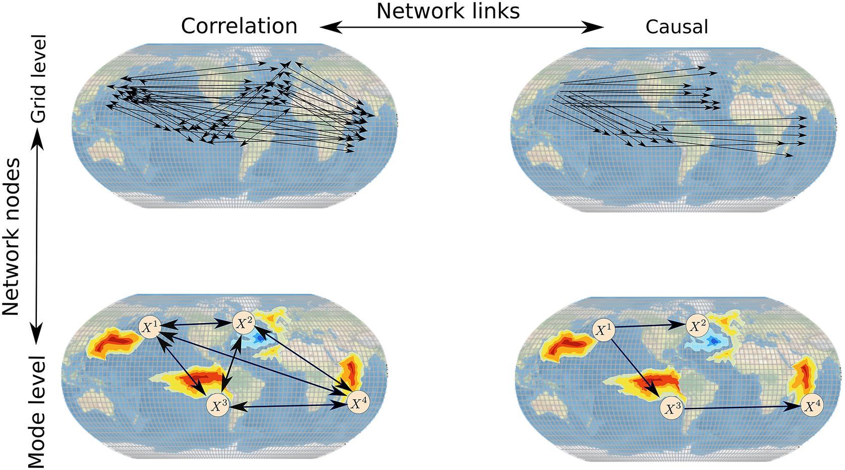
(Tibau et al., 2022) presented a spatiotemporal stochastic climate model SAVAR which can be used to benchmark causal discovery methods for teleconnections, providing insights into the strengths and weaknesses of different analysis methods. The authors also introduced novel causal discovery method named Mapped-PCMCI that outperforms existing approaches, contributing to the advancement of process-based understanding and climate model evaluation. The proposed SAVAR model benchmarks different teleconnection analysis methods including grid-level causal discovery methods and a combination of dimension-reduction and causal discovery methods. The experiments conducted in the paper demonstrate that the grid-level causal method based on the SAVAR model outperforms baseline causal discovery methods, which do not consider the mode structure and attempt to directly infer the causal graph at the grid level. Proposed with the SAVAR is the Mapped-PCMCI method, which is based on the assumption that the causal dependencies within a gridded dataset have a lower-dimensional mode representation. The method consists of four steps (Figure 5): (1) Perform a dimensionality reduction method on the gridded data to extract a limited number of mode time series variables. (2) Apply a causal discovery method to the mode time series variables to obtain the parents and the estimated causal network of the modes. (3) Estimate (lagged) causal effects for all links to obtain a coefficient matrix. (4) Invert the dimension reduction by mapping the causal effects among the grid locations using the modes’ weights. This method aims to overcome the challenges of dealing with large networks, nonstationary networks, and the high-dimensional and redundant estimation problem at the grid level. It provides a spatial grid-level representation of the causal network obtained at the mode level, allowing for the analysis of causal relationships in complex systems. Python code for both the SAVAR and Mapped-PCMCI were published on GitHub 888https://github.com/xtibau/.
3.5.2 Interactive Causal Structure Discovery (ICSD)
(Melkas et al., 2021) presented a workflow ICSD (Interactive Causal Structure Discovery) in Earth System Sciences that takes into account experts’ domain knowledge during the application of causal discovery (CD) algorithms in Earth sciences systems. ICSD provides users an interactive way to edit the outputs of different CD algorithms and iteratively incorporate prior knowledge in the initial output models. It formulates the structure learning problem as building a probabilistic model of the data and encodes expert’s prior knowledge as a prior distribution over all possible causal structures. The current formulation takes a greedy approach which leads to local optima where the choice of the initial state affects the final model. A score is associated with each causal model that reflects the log-likelihood of the model. For demonstration of the approach, three different CD algorithms (PC, GES and LiNGAM) were experimented on a forestry dataset that includes daytime measurements of variables such as shortwave downward radiation, temperature, latent heat flux vapor, pressure deficit, etc. Experimental results suggest that even a small amount of prior knowledge is useful in improving the results of CD algorithms. The experiments also showed how overfitting and concept drift can occur and be detected by ICSD. At present, the user navigation begins with the outputs from different CD algorithms which is sub-optimal. A future work is to find an optimal set of representative starting points for exploration.
3.5.3 Spatio-Temporal Causal Discovery Framework(STCD)
The Spatio-Temporal Causal Discovery Framework (STCD) (Sheth et al., 2022) aimed to identify causal relationships in the spatio-temporal domain by enforcing both temporal and spatial constraints. This framework is motivated by the influence of causal factors in hydrological systems where the geographical location of a river or a subsidiary is a crucial factor in deciding the causal parents. STCD primarily extends the TCDF (Nauta et al., 2019b) framework by adding a component that ensures the enforcement of the spatial constraint. TCDF is a temporal causal discovery approach based on CNNs for multivariate time series data that uses an attention mechanism to identify potential causal parents of the target time-series. Using the attention scores, it filters the list of potential candidates. The proposed framework STCD on the other hand eliminates irrelevant candidates by penalizing the attention scores if the candidates violate the spatial constraints. When the attention vector for a target time series is obtained, then the spatial constraint is imposed on it. In hydrological systems, a river located geographically below the target river can never be a causal parent even if they satisfy the temporal constraint because the flow of water is always from top to bottom. Motivated by this idea, the spatial constraint imposes a direction of the flow. Specifically, it is the product of a distance and a spatial coefficient . The distance has either a positive or negative direction based on the geographical positioning of the locations, and controls the effect of the spatial constraint on the attention score. The framework is tested to discover causal relationships of streamflow at the mouth of the Brazos basin in Texas from runoff in the basin. A limitation of STCD is that it models the spatial and temporal interactions separately which might hinder the discovery process when the spatial and temporal components influence each other.
3.5.4 Group Elastic Net
(Lozano et al., 2009) proposed a data-centric approach to climate change attribution, using spatial-temporal causal modeling to analyze climate observations and forcing factors. The authors developed a novel method called Group Elastic Net to infer causality from the data and incorporate extreme value modeling to study extreme climate events. With the assumption of spatial stationarity, the model combines graphical modeling techniques with Granger Causality to derive effective methods for causal modeling based on the spatio-temporal structure of the data and enforces sparsity at the group level. The model also applies extreme-value theory to model extreme events and incorporates these estimates into the causal modeling and attribution process. The experiments involve data collection from multiple sources. For real data collection, the researchers compiled a comprehensive set of relevant variables for climate modeling in North America. They obtained data from various sources including the Climate Research Unit (CRU), the National Oceanic and Atmospheric Administration (NOAA), NASA, the National Climate Data Center (NCDC), and the Carbon Dioxide Information Analysis Center (CDIAC). These sources provided data on climate variables such as temperature, precipitation, solar irradiance, greenhouse gases, and aerosols. In addition to the real climate data, the researchers also conducted simulation experiments using synthetic spatial-temporal data. They used a spatial-temporal vector autoregressive (VAR) model to generate the synthetic data. The experiments compared the performance of the Group Elastic Net method, which considers spatial interactions, with a method that neglects such interactions. The experimental results indicate that changes in temperature are not solely accounted for by solar radiance but are attributed more significantly to CO2 and other greenhouse gases. The results also show a significant increase in the intensity of extreme temperatures, and these changes are attributable to greenhouse gases. The proposed approach offers a useful alternative to simulation-based climate modeling and provides valuable insights from a fresh perspective.
3.5.5 pg-Causality
Previous methods for identifying causal pathways in air pollution have been proposed from two perspectives: pattern-based and Bayesian-based. Pattern-based approaches provide shallow understanding and have limited usability due to a large number of patterns, while Bayesian-based approaches are limited by noise, data sparsity, computational cost, and confounding factors. Zhu et al. (Zhu et al., 2017) present a novel approach, called pg-Causality, which combines pattern mining and Bayesian learning to efficiently identify spatiotemporal causal pathways for air pollutants using urban big data. The approach overcomes the challenges of noise, computational complexity, and complex causal pathways, and thus outperforming traditional methods in terms of time efficiency, inference accuracy, and interpretability. The authors use the FEP Mining Algorithm to mine frequent episode patterns (FEPs) in a symbolic pollution database. This algorithm considers constraints such as consecutive symbols being different and a specified temporal constraint between consecutive records. After discovering the FEPs, the authors extract candidate causes for each sensor by finding pattern-matched pairs within a specified time lag threshold. The authors use a Gaussian Bayesian network (GBN) based graphical model to capture the causal relationships among air pollutants. They generate initial causal pathways by incorporating the extracted matched patterns and candidate sensors into the GBN model. Finally, the authors refine the causal structures using an EM learning phase and a structure reconstruction phase. The EM learning phase learns the parameters of the graphical model, while the structure reconstruction phase selects the top neighborhood sensors based on the newly generated GCscore and updates the Q matrix. The experiments were conducted using real-world data sets from North China, Yangtze River Delta, and Pearl River Delta. These data sets included records of 6 air pollutants and 5 meteorological measurements. The approach showed scalability in identifying causal pathways for air pollutants at the sensor level, which is more than ten times larger than at the city level. The overall experimental results showed that the proposed approach achieved high accuracy, time efficiency, and scalability in inferring causal relationships in air pollution data.
3.6 Applications of Causal Discovery in Earth Science
We explained some of the renowned causal discovery methods for time-series and spatiotemporal data in the previous subsection. Here, we will share some of the applications of those widely used causal discovery methods, specifically in the Earth Science domain. A summary of these applications is provided in Table 6.
| Data | Method | Application |
| Time-series | PC | Causal discovery for hydrometeorological systems (Ombadi et al. 2020) |
| GC | Long-term causal links in climate change events (Smirnov and Mokhov 2009, Kodra et al. 2011) | |
| GC | Causal discovery for hydrometeorological systems (Ombadi et al. 2020) | |
| GC | Causal discovery for teleconnections (Mosedale et al. 2006, Varando et al. 2021) | |
| CEN | Causal discovery for midlatitude winter circulation within the Arctic (Kretschmer et al. 2016) | |
| CEN | Causal discovery for precursors of september Arctic sea-ice extent (Li et al. 2018) | |
| PCMCI | Causal discovery for biosphere–atmosphere interactions (Krich et al. 2020) | |
| PCMCI | Causal discovery to study wildfire impact (Qu et al. 2021) | |
| Causal Feature Learning | Causal discovery for teleconnections (Chalupka et al. 2016) | |
| Tidybench Algorithms | Causal discovery for time-aggregation, time-delays and time-subsampling in | |
| weather data (Weichwald et al. 2020) | ||
| Spatiotemporal | PC-stable | Spatiotemporal causal discovery for univariate climate data (Ebert-Uphoff and Deng 2017) |
| PCMCI | Causal discovery for tropical–extratropical summer interactions (Di Capua et al. 2022) | |
| Mapped-PCMCI | Causal discovery for teleconnections (Tibau et al. 2022) | |
| STCD | Causal discovery for hydrological systems (Sheth et al. 2022) | |
| Group Elastic Net | Causal discovery for climate change attributions ((Lozano et al. 2009) | |
| pg-Causality | Identifying causal pathways for air pollutants (Zhu et al. 2017) |
3.6.1 Applications of Granger Causality
In climate research, understanding complex phenomena, such as teleconnection patterns, is important because it links atmospheric changes in one region to impacts in distant regions. However, the automatic identification of these patterns from observational data is still unresolved due to nonlinearities, nonstationarities, and the limitations of correlation analyses. Varando et al.(Varando et al., 2021) propose a deep learning approach to address these problems and learn Granger causal feature representations that capture the true causal effects of the target index, such as El Niño Southern Oscillation (ENSO) or North Atlantic Oscillation (NAO). The authors propose a method called the Granger Penalized Autoencoder with the assumptions including the presence of nonlinearities and nonstationarities in the observational data, as well as the limitation of correlation analyses in identifying true causal patterns. By utilizing normalized difference vegetation index (NDVI) data collected from MODIS reflectance data over 11 years, their work identified clear patterns of the causal footprints of ENSO on vegetation in different regions. The GitHub repository of this research is approachable999https://github.com/IPL-UV/LatentGranger. (Mosedale et al., 2006) used a Granger causality based approach to quantitatively measure the feedback of daily sea surface temperatures (SSTs) on daily values of the North Atlantic Oscillation (NAO). This was done by simulating a realistic coupled general circulation model (GCM). This study is an extension of the work by Mosedale et al. in 2005. where the Granger causality approach is used to find the best time series models for modeling the coupled system for greater flexibility. (Smirnov and Mokhov, 2009) introduced the idea of long-term causality, which is an extension of Granger causality. Long-term causality was estimated from data through empirical modeling and analysis of model dynamics under different conditions. They applied this concept to find out how strongly the global surface temperature (GST) is affected by variations in carbon dioxide, atmospheric content, solar activity, and volcanic activity during the last 150 years. (Kodra et al., 2011) extended the classic Granger causality test to handle the multisource nature of data. Using a reverse cumulative Granger causality test, they tested the hypothesis that Granger causality can be extracted from the bivariate series of globally averaged land surface temperature (GT) observations and observed CO2 in the atmosphere.
3.6.2 Applications of Pearl Causality
Causal discovery algorithms based on probabilistic graphical models have been applied in geoscience applications to identify and visualize dynamical processes, but the lack of ground truth and unexplained connections have posed several challenges. To address these challenges, Ebert-Uphoff et al.(Ebert-Uphoff and Deng, 2017) developed a simulation framework using synthetic spatio-temporal data to better understand the physical processes and interpret the resulting connectivity graphs, ultimately solving the mystery of the previously unexplained connections. This approach allows for the resolution of previously unexplained connections and provides a benchmark for other causal discovery algorithms. The authors used a constraint-based structure learning method called the PC stable algorithm, which is a modification of the classic PC algorithm. This algorithm produces graph structures where observed variables form the nodes, and connections between nodes indicate potential cause-effect relationships. The PC stable algorithm has advantages such as increased robustness of results and suitability for parallelization. The authors dropped the requirement of causal sufficiency and focused on necessary conditions for cause-effect relationships. The article discusses the results of three different scenarios in the simulations. In Scenario 1, increasing the spatial resolution leads to more edges for a specific time interval and fewer edges for a longer time interval. In Scenario 2, concurrent edges are believed to be caused by contradictory velocities at the boundaries of the advection field. In Scenario 3, concurrent edges in the center do not match the typical diffusion pattern and appear to fill modeling gaps. The velocity estimates in Scenario 1 with higher speed are weak due to many high-speed interactions represented as concurrent edges.
3.6.3 Applications of PCMCI
(Krich et al., 2020) used the PCMCI algorithm to study the underlying causal relations in biosphere–atmosphere interactions. Particularly they estimated the causal graphs from the eddy covariance measurements of land–atmosphere fluxes and global satellite remote sensing of vegetation greenness datasets. The causal graphs revealed the gradual shifts that correspond to little adjustments, such as the relationship between temperature and visible heat as well as increasing dryness which might not have been discovered merely through correlation analysis.
(Qu et al., 2021) used PCMCI to recover the causal graphs for 8 vegetation types which represent the causal relations and time lags between wildfire burned areas and weather/drought and vegetation conditions. A significant conclusion they found is that weather and aridity conditions are dominant indicators to burned areas for grassland. Also, for broadleaf forests, radiation while for needleleaf forests temperature is the most vital indicator. To analyze the influence of a set of spatial patterns representing tropical–extratropical summer interactions, (Di Capua et al., 2022) estimated causal maps which is an extension of PCMCI to spatial fields of variables.
Lastly, given the challenges in analyzing teleconnections and the lack of ground truth benchmark datasets, Mapped-PCMCI(Tibau et al., 2022) proposed to tackle these challenges by presenting a simplified stochastic climate model that generated gridded data and represents climate modes and their teleconnections.
3.6.4 Applications of other Causal Discovery Methods
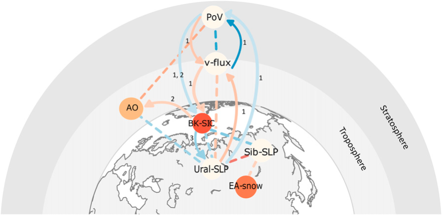
One of the predecessors of PCMCI method is the Causal Effect Network (Kretschmer et al., 2016) which was implemented to identify the time-delayed causal relationships between different actors of midlatitude winter circulation within the Arctic. Through experiments on monthly, bi-monthly and quarter-monthly time-series of seven meteorological variables (See (Kretschmer et al., 2016) for details), the authors pin-pointed Barents and Kara sea ice to be important drivers of winter circulation further confirming the troposphere-stratosphere coupling proposed in previous literature. The causal graph of this discovery is given in Figure 6. The same approach was utilized by (Li et al., 2018) to study the precursors of summer (September) Arctic sea-ice extent.
(Chalupka et al., 2016) learned macro-level causal features from micro-level variables without supervision using Causal Feature Learning (CFL). These macro-level features are used to discover causal relationships between them and target output. Aggregating micro-level variables into the macro-level variables helps to ignore changes in the micro-level variables that have no effect on the output variable Y. Here the authors calculated conditional expectation using the regression of Y based on x. Then these conditional expectations are clustered to generate the macro-level variables. This method was used to find the causal relation between the El Nino and La Nina events with the eastern Pacific near-surface wind (ZW, zonal wind) and sea surface temperature (SST) variable.
(Ombadi et al., 2020) aimed to evaluate different causal discovery methods and their performance in retrieving causal information from synthetic data and real-world observations for hydrometeorological systems. The methods for causal discovery in hydrometeorological systems involved in the paper are Granger causality (GC), Transfer Entropy (TE), graph-based algorithms (PC), and Convergent Cross Mapping (CCM). The author applies them to examine the causal drivers of evapotranspiration in a shrubland region during summer and winter seasons. The study aims to present the fundamentals of these methods and shed light on their assumptions in the context of hydrometeorological systems. Specifically, it discusses the assumptions of causal sufficiency, causal faithfulness, and stationary time series. To evaluate performance of the four causal discovery methods, the study uses synthetic data generated from the bucket model and analyzes the causal structures of hydrological systems. The evaluation includes assessing the asymptotic performance of each method, investigating the sensitivity to sample size, and assessing the sensitivity to the presence of noise. The observational data is obtained from the Santa Rita Mesquite FluxNet site in Arizona to analyze the environmental controls on evapotranspiration.
4 Causal Inference
Causal inference can be defined as the process of estimating the causal effects (influence) of one event, process, state or object (a cause) on the another event, process, state or object (an effect). Causal inference has been applied to study environmental science for several decades, with early applications dating back to the mid-20th century (Hill, 1965). However, much of the earlier causal inference based analysis was done on independent and identically distributed (i.i.d) data utilizing statistical inferential and regression techniques to estimate the causal effects on potential outcomes (Pearl, 2009). This section presents the key terminologies (Table 7), common approaches and causal assumptions required to perform causal inference techniques. We explain the different time-series and spatiotemporal causal inference techniques introduced, along with their limitations and applications in Earth Science.
| Terminology | Explanation |
|---|---|
| causal effect | strength or infleunce of a causal relation |
| instance | a single unit; data sample |
| treatment | cause; variable that is intervened on |
| potential outcome | effect; variable exposed to the treatment |
| confounders | variable influencing both treatment and outcome |
| covariates | pre-treatment variables; features |
| intervention | nudging the value of a treatment variable |
| average treatment effect (ATE) | the average difference in potential outcomes with and without |
| undergoing intervention |
4.1 Common Approaches
For estimation of causal effect, there are two main categories of techniques, potential outcome framework and do-calculus.
4.1.1 Potential Outcome Framework:
The potential outcome framework relies on hypothetical interventions such that it defines the causal effect as the difference between the outcomes that would be observed with and without exposure to the intervention. This technique is widely used in epidemiology where patients are randomly divided into treated and controlled groups and the effectiveness of treatment is inferred by observing patients condition with and without undergoing a treatment (Rubin, 2005). The treatment effect can be measured at individual, treated group, sub-treated group and entire population levels.
4.1.2 Do-Calculus
The first method, do-calculus was developed in 1995 to identify causal effects in non-parametric models using conditional probabilities (Spirtes, 2010). Once a causal structure is identified, do-calculus can be applied to find interventional distributions by deriving mathematical representations for a physical intervention using the operator, as shown in Equation 4. Here, Y represents the outcome, X represents the variable intervened on and Z represents a set of covariates.
| (4) |
In case of a binary-valued variable X, the average causal effect (ACE) can be calculated using do-calculus by calculating the difference between do(X=1) and do(X=0), as shown in Equation 5.
| (5) |
4.2 Assumptions for Causal Inference
For consistent causal effect estimation on observational data, it is important to hold the following identifiability conditions or causal assumptions:
Consistency:
Under the consistency condition, the potential outcome for the treated subject is considered equal to the observed outcome Y. The same goes for the untreated subject.
Positivity:
This assumption implies that the probability of receiving treatment given some covariates is always greater than zero. That is, where .
Conditional Exchangeability:
Under the conditional exchangeability assumption, also known as ”weak ignorability”, the condtional probability of receiving treatment depends only on the covariates , that is, and treatment are are statistically independent given every possible value of . On the contrary, unconditional exchangeability implies that treatment group has the same distribution of outcomes as the untreated control group.
SUTVA:
Under the Stable Unit Treatment Value Assumption (SUTVA), the potential outcome on one unit is not affected by the treatment effect on other units and there is no hidden variations of treatment.
4.3 Evaluation Metrics
4.3.1 Root Mean Square Error (RMSE)
Researchers evaluate the performance of their predictive models using the Root Mean Square Error (RMSE) which can be only calculated for factual observational data but cannot be done for counterfactual predictions. Since the ground truth information is only available for synthetic data, we further evaluate the causal effect estimation skill of a model using the PEHE metric.
| (6) |
4.3.2 Precision in Estimated Heterogeneous Effects (PEHE)
This metric is commonly used in machine learning literature for calculating the average error across the predicted average treatment effects (ATEs) (Hill, 2011).
| (7) |
4.4 Time-series Causal Inference
Majority of the causal inference models work in time and space invariant settings. However, when it comes to time-series data, the question changes to inferring the effect of treatment on outcome at time in the presence of a set of covariates . Such settings require models that can estimate time-varying causal or treatment effects. This further leads to the problem of time-varying confounding, that is the common influence a past treatment or covariate might have on the future treatments and the future outcome . Traditional methods for performing time-series causal inference typically involve statistical modeling techniques that aim to identify causal relationships between variables in time-series data, however, these methods have several limitations, which can affect the reliability and validity of causal conclusions drawn from the analysis.
In causal inference, confoundedness poses a significant challenge because it can lead to incorrect conclusions about the causal relationship between the independent variable and the dependent variable. When confounding variables are not properly accounted for, the observed association between the independent and dependent variables may be due to the confounding variable rather than a true causal effect. Balancing scores that incorporate propensity score are the most common approaches to debias confounding effects. To overcome this challenge, Robin’s g-methods have shown to provide promising results on reducing bias caused by time-varying treatment and covariates on the potential outcome (Naimi et al., 2017). The prediction models of these estimators are typically based on linear or logistic regression, the downside of which is that in case of complex non-linearities in treatment or outcome variables, these methods will lead to inaccurate results. G-methods provide metrics to overcome the problem of time-varying confounding through standardization, g-computation and inverse probability of treatment weighted (IPTW) estimators (Naimi et al., 2017).
4.5 Time Series Causal Inference Methods
So far, we have seen causal inference surveys focusing on CI methods for i.i.d. data (Table 1), however, real world observations require dynamic or time-varying causal analysis focusing on calculating the impact of an intervention on a sequential or time-varying outcome (Moraffah et al., 2021). For instance, policymakers and climate change activists would be interested in identifying the impact of lowering CO2 emissions on the rate of ozone depletion over a specific period of time. Depending upon the underlying methodology, time-series causal inference methods can be categorized into (i) time-varying causal inference, and (ii) time-invariant causal inference methods. We summarize some of the widely-used causal inference methods under each category below.
4.6 Time-varying Causal Inference Methods
Time-varying causal inference methods are approaches used to understand and analyze causal relationships in situations where the treatment or intervention, the outcome, and potentially the covariates, change over time. These methods aim to uncover how a changing treatment influences the outcome of interest, considering the dynamic nature of both the treatment and the outcome variables.
In contrast to traditional causal inference, where the focus is on a fixed intervention and its effect, time-varying causal inference takes into account the evolving nature of interventions and outcomes. This is particularly relevant in fields such as epidemiology, economics, and environmental science, where interventions and exposures can vary over time. Some common time-varying causal inference methods include:
4.6.1 Marginal Structural Models
Marginal Structural Models (MSMs) (Robins et al., 2000) are a class of causal inference methods designed to estimate the causal effects of time-varying treatments in the presence of time-dependent confounding. While traditional methods like ordinary regression models may not properly handle time-varying treatments and confounders, MSMs were developed to address biases that can arise when using these traditional regression models to estimate causal effects in situations where treatments change over time. MSMs provide a framework to model and adjust for the dynamic nature of treatments, confounders, and their interdependencies using the IPTW weights. MSMs first employ IPTW to re-weight the data and emulate a hypothetical time-fixed treatment scenario. This mitigates confounding by making treated and untreated groups comparable. A weighted regression model is then employed to estimate the treatment effect, accounting for the dynamic confounding. MSMs rely on the assumptions of positivity and no unmeasured confounders. Though MSMs have become a cornerstone in time-varying causal inference in the fields of epidemiology (VanderWeele, 2009; Hernán et al., 2000), public health (Williamson and Ravani, 2017; VanderWeele et al., 2011) and social sciences(Bacak and Kennedy, 2015), they also have some limitations. Complex interactions between time-varying treatments and confounders, longitudinal missing data and information censoring can be challenging to model using MSM technique.
4.6.2 Convergent Cross Mapping
Convergent Cross Mapping (CCM) (Ye et al., 2015) is a nonlinear causal inference technique used to detect the presence of causal relationships between variables in time series data. It is particularly useful when the relationship between variables is complex and non-linear. CCM is based on the concept of time delay embedding, where time series data is transformed into higher-dimensional space by embedding time-delayed copies of the series.
4.6.3 Instrument Variables
In causal graphs, a variable is called an instrumental variable (IV) if it is independent of the hidden confounders and related to the effect only through the cause. For a causal model of the form prediction of the Y based on the observation X with the presence of hidden confounders yields a biased estimation of the coefficient. The Conditional Instrumental Variable (CIV) (Thams et al., 2022) method used IVs to identify the coefficient from the time series causal model with the presence of hidden confounders applying condition on the required number of previous instances of IVs.
4.6.4 Deep Representation Learning based Models
Causal inference methods based on representation learning or deep learning techniques (Bengio et al., 2013) learn the representation of input data by extracting features from the covariate space (Koch et al., 2021), where majority of the existing deep learning based methods are developed for i.i.d data (Koch et al., 2021). In these deep learning based CI methods, a single neural network (also called meta learner) can be trained to make predictions for both treatment and control groups individually to estimate the average treatment effect (ATE).
For time-series causal inference, researchers have proposed methodologies based on machine learning and deep learning models that also tackle the problem of time-varying confounding (Moraffah et al., 2021). Recurrent Marginal Structural Networks (R-MSN) (Lim, 2018) and Counterfactual Recurrent Network (CRN) (Bica et al., 2020b) are some of the recent models that claim to estimate causal effects in the presence of time-varying confounders, however, contrary to the claim, these methods are healthcare-specific and cannot be generalized for other domain areas like Earth science because these models require one-hot encoded treatment flags with multivariate combined dosage. Time Series Deconfounder - a multi-task method, leverages the assignment of multiple binary treatments over time to enable the estimation of treatment effects in the presence of multi-cause hidden confounders (Bica et al., 2020a). Taking this one step further, G-Net is a recently proposed method for time-varying dynamic treatment effect estimation (Li et al., 2021b). The method provides a recurrent-neural network based g-computation technique to estimate the propensity scores for handling time-varying confoundedness. Most recently, (Ali et al., 2023) proposed TCINet, a deep learning based counterfactual prediction model that leverages stabilized weighting (instead of IPTW weights) using probabilistic modeling. The authors evaluated TCINet on climate data and presented their findings on the relationship between Greenland blocking and summer sea ice melt within Barents Sea and Kara Sea.
Though deep representation learning methods are capable of automatically learning the intrinsic correlations and are also effective in accurate counterfactual estimation, they often lead to predictions with high variance or uncertainty estimates.
4.7 Time-invariant Causal Inference Methods
Time-invariant treatment effect estimation methods focus on quantifying the causal impact of a treatment on an outcome when both the treatment and outcome variables are observed at a single point in time. Whereas, a treatment is time-invariant or fixed when it occurs at one specific point of time and then does not change afterwards. We enlist some of the time-invariant causal inference methods below:
4.7.1 Causal-ARIMA
The Causal-ARIMA (C-ARIMA) is a potential outcome framework-based method to estimate causal effects from time series datasets (Menchetti et al., 2021). This method is suitable for datasets where it is not possible to separate the treated and controlled groups to estimate the effects of the applied treatment. In an observational study, if an intervention event occurs at a specific time point, the time series divides into two different time horizons, pre-intervention and post-intervention. Here the intervention is not applied at each time point, it occurred at a given time and draws the effect on the rest of the observations of the system. The C-ARIMA method is a three-step process: first, the relationship between the covariates and target variable is learned from the pre-intervention data using an ARIMA model. Then using learned relationships from pre-intervention data the counterfactual outcomes are predicted for post-intervention data points. Finally, the causal effect is measured from the factual observations and predicted counterfactual data. The C-ARIMA method works on the basis of five assumptions: single persistent intervention, non-anticipating potential outcomes, temporal no-interference, covariates-treatment independence, and Non-anticipating treatment. The C-ARIMA method can identify different types of causal effects without making any structural assumptions about the effect caused due to the intervention.
4.7.2 Difference in Difference
The Difference-in-Differences (DID) method (Lechner, 2011) is a statistical technique used in econometrics and social sciences to estimate the causal impact of a treatment, intervention, or policy by comparing changes in outcomes over time between a treatment group and a control group. DID is particularly useful when randomization of subjects into treatment and control groups is not possible or ethical, making it challenging to establish causality through traditional experimental methods. To perform causal inference using this method, start by selecting two groups: a treatment group that is exposed to the intervention or policy change and a control group that is not exposed. These groups should be similar in all relevant aspects except for the treatment or policy change. Next, data is collected on the outcome of interest for both groups, typically before and after the treatment or policy change. Finally, the causal effect is estimated by calculating the difference in the changes in outcomes in the controlled group and the treated groups. The DID estimate can be analyzed using regression techniques to control for potential confounding factors, such as demographics or other trends affecting the outcome. However, there are some limitations. The method requires adequate sample size to yield meaningful results and it can handle time-varying confounders. Overall, Difference-in-Differences is a powerful tool for causal inference when randomized controlled trials are not feasible or ethical. However, it relies heavily on the validity of the parallel trends assumption, and researchers must carefully consider potential sources of bias when designing and interpreting DID studies. Mathematically, the DID estimate can be expressed as follows:
| (8) |
Here, refers to the outcome in treated group, refers to the outcome in the controlled group, refers to the pre-treatment data and refers to post-treatment data.
4.7.3 Interrupted Time Series
Interrupted time series (ITS) analysis (McDowall et al., 1980) is a statistical method used for assessing the causal impact of an intervention, treatment, or policy change on a specific outcome by analyzing changes in a time series data set. Unlike the Difference-in-Differences (DID) method, which compares two groups (treatment and control) before and after an intervention, ITS focuses on a single group and tracks changes in that group’s outcomes over time, before and after the intervention. ITS requires defining a point in time when the intervention, treatment, or policy change occurred. This is referred to as the ”interruption point”. A statistical model is built to estimate the expected trajectory of the outcome in the absence of the intervention. Common models used for pre-intervention estimation include linear regression, autoregressive integrated moving average (ARIMA), or segmented regression models. To estimate the effect of the intervention, observed outcomes after the intervention are compared with the predicted outcomes from the model. The difference between the observed and predicted outcomes at each time point after the intervention represents the intervention effect.
Interrupted time series analysis is particularly valuable for evaluating the impact of policies, interventions, or treatments that are implemented at a specific point in time. It provides a rigorous framework for establishing causal relationships by demonstrating that observed changes in the outcome are more likely due to the intervention than to other factors. However, as with any statistical method, the validity of ITS analysis depends on the quality of data and the appropriate modeling of the pre-intervention trend. ITS can be a powerful tool for causal inference when experimental designs are not feasible.
4.7.4 Causal Impact
The Causal Impact method (Brodersen et al., 2015) is a statistical approach used for estimating the causal effect of an intervention, event, or treatment on a time series data set. It was developed by Google’s Research and Data Science teams and is implemented in the R package (http://google.github.io/CausalImpact/CausalImpact.html). This method is particularly useful for businesses and researchers to assess the impact of marketing campaigns, policy changes, or any other interventions on metrics such as sales, website traffic, or user engagement. The Causal Impact method builds a Bayesian structural time series (BSTS) model to represent the expected behavior of the time series data in the absence of the intervention. The BSTS model captures trends, seasonality, and other patterns in the pre-intervention data. The difference between the observed post-intervention data and the counterfactual prediction represents the causal impact of the intervention. This difference is used to estimate the treatment effect and assess its statistical significance. Causal Impact is particularly valuable when you want to assess the impact of a specific event or intervention on a time series metric while accounting for the underlying patterns and variations in the data. It offers a probabilistic and data-driven approach to causal inference, which can be beneficial for decision-making in various domains.
4.7.5 Regression Discontinuity Design
The Regression Discontinuity Design (RDD) method (Hahn et al., 2001) is a quasi-experimental research design used in causal inference to estimate the causal effect of a treatment, intervention, or policy change when the assignment to the treatment or control group is determined by a cutoff or threshold in a continuous or ordinal variable. RDD is particularly useful when random assignment to treatment and control groups is not feasible, but there exists a natural ”discontinuity” in the assignment process that can be exploited to make causal inferences. RDD is a powerful method for causal inference when the assignment to treatment or control groups is determined by a discontinuity in a continuous or ordinal variable. However, it relies on the assumption of a smooth discontinuity and requires careful design and analysis to ensure valid causal inferences.
RDD estimates the treatment effect using regression analysis. The method requires defining a threshold in the data . The ATE is estimated by comparing the average outcomes for individuals just below the threshold with those just above the threshold . The difference in outcomes between the two groups can be attributed to the treatment or intervention. Mathematically, the ATE estimate can be expressed as follows:
| (9) |
| Method |
|
|
|
|
|
||||||||||
|---|---|---|---|---|---|---|---|---|---|---|---|---|---|---|---|
| Difference in Difference | \cmark | \xmark | \xmark | \xmark | \xmark | ||||||||||
| Causal Impact | \cmark | \cmark | \cmark | \xmark | \cmark | ||||||||||
| Instrument Variables | \cmark | \cmark | \cmark | \cmark | \cmark | ||||||||||
| CRN | \cmark | \xmark | \cmark | \cmark | \xmark | ||||||||||
| MSM | \cmark | \xmark | \cmark | \xmark | \xmark | ||||||||||
| R-MSN | \cmark | \xmark | \cmark | \cmark | \xmark | ||||||||||
| Time-series Deconfounder | \cmark | \xmark | \cmark | \cmark | \xmark |
4.8 Spatiotemporal Causal Inference
Methods for spatiotemporal causal inference often integrate techniques from both causal inference and spatiotemporal analysis. These methods may include statistical modeling, machine learning algorithms, and deep learning approaches to estimate causal effects in observational data while considering spatial and temporal dependencies. Reich et al. provided a comprehensive review of the challenges and limitations of performing causal inference in spatial settings and enlisted methods that exploit spatial structure and those that account for spatial interference in spatiotemporal settings (Reich et al., 2021). Here, we present some of the recent methods introduced to perform causal inference on spatiotemporal data.
4.8.1 Spatially Interrupted Time-Series (SITS)
(Zhang and Ning, 2023) investigated the spatiotemporal heterogeneities in the causal effects of mobility intervention policies during the COVID-19 outbreak using a spatially interrupted time-series (SITS) analysis. The study aimed to understand the spatiotemporal heterogeneity in the causal effectiveness of these policies, particularly at finer-grained spatial and temporal resolutions, and provide insights for policymakers on when and where to implement specific policies to control the spread of the virus. The SITS system involves the application of the Interrupted Time-Series (ITS) design combined with spatial analysis. The ITS design is a quasi-experimental design for policy evaluation that records and measures behavioral outcomes before and after implementing a policy intervention. The SITS analysis requires a long time series with multiple observations over time, especially before the treatment period, to establish a credible estimation of counterfactuals. It compares mobility outcomes over time within a single group of individuals or neighborhoods, rather than between a treatment group and a control group. This helps to control for potential biases arising from between-group differences. To incorporate spatial heterogeneities, the SITS analysis considers the spatial contexts of neighborhoods, including socioeconomic and built environment settings. The effects of the policy intervention, such as the level and slope changes, are moderated by these spatial contexts. The SITS model estimates the spatiotemporally varying causal effects of the policy interventions by incorporating these spatial moderating effects. The SITS analysis in this study used a timeseries dataset of neighborhood-based mobility levels extracted from a large set of mobile phone signaling data in Shenzhen, China. The dataset allowed for tracking the daily mobility trend at the neighborhood level before and after the COVID-19 outbreak. Two mobility control policies were focused on: the first-level response to public health emergencies (FLR) declared on January 23, 2020, and the lockdown of residential communities (COM) implemented on February 7, 2020. By revealing the disparities in the ability to alter normal activity patterns in response to NPIs, the study also provides insights into sociospatial equality and resilient neighborhood planning in the post-epidemic era. The study analyzed the effects of two mobility intervention policies: the first-level response (FLR) policy and the closed-off management (COM) policy. The spatial distributions of the decay rates of the two policies were different, with neighborhoods with larger decay rates primarily located in compact areas near city centers for the FLR and at the urban fringe for the COM. The study also found that the spatial variations in mobility change became increasingly small or homogenous over time.
4.8.2 Propensity Score based Spatiotemporal Causal Inference Methods
Propensity scoring techniques are extended in spatiotemporal causal inference setting to account for confounding caused by spatial confounders. Papadogeorgou et. al. proposed a distance adjusted propensity score method to incorporate spatial proximity in causal inference techniques in the presence of observed confounders (Papadogeorgou et al., 2019). Later, they proposed a spatiotemporal causal inference method for stochastic interventions assuming both the treatment and outcome variables are coming from the spatiotemporal point processes (Papadogeorgou et al., 2022). In the stochastic intervention setting the treatments are specified through a probability distribution instead of fixed values in the potential outcome framework. This model makes two assumptions on the treatment: unconfoundedness and bounded relative overlap of the treatment, which ensures that the intervention with high probability does not become a fixed treatment. This method allows the intervention can be applied to any spatial location, an infinite number of interventions at the same time and measures the outcome for all applied interventions using an intervention distribution pattern. So it is possible to apply and measure the outcomes for any spatial and temporal intervention patterns.
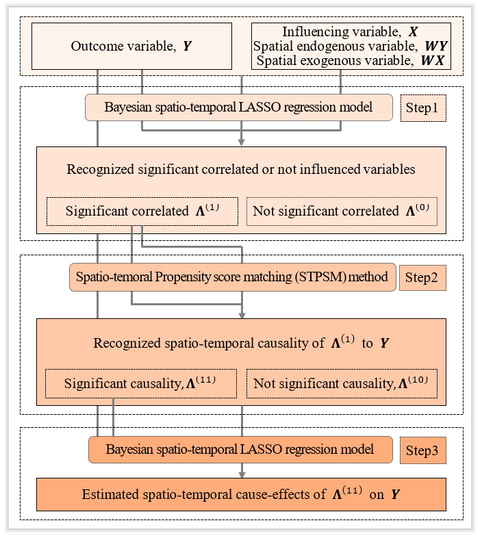
4.8.3 Additional Spatiotemporal Causal Inference Methods
Christiansen et al. proposed a latent spatial confounder model to study relationship between conflict and the forest loss in Columbia (Christiansen et al., 2022). Papadogeorgou et al. recently proposed a Bayesian modeling approach to causal inference in the presence of latent confounders and spatial interference (Papadogeorgou and Samanta, 2023). Overall, spatiotemporal causal inference still remains a lesser tapped area with much focus on spatiotemporal causal structure learning (part of spatiotemporal causal discovery). One reason behind this is the challenging task of inferring causation in both space and time-varying setting in the presence of latent confounders and spatial interference, two of the major challenges in this research area.
4.9 Applications of Causal Inference in Earth Science
Applications of causal inference in Earth Science is constrained by the inability of validating the findings as observational data cannot be controlled, randomized or intervened on. Nevertheless, we enlist some of the recent inroads in causal inference for Earth Science domains. (Yang et al., 2022) applied an advanced data-driven causal inference method based on the convergent cross mapping (CCM) algorithm that provides valuable insights to identify thermal influence and feedback among the different climate regions in the contiguous U.S using the long-term (1901–2018) near surface air temperature observations. (Gao et al., 2022) studied some widely applied causal inference approaches to study the extent of the influence of different vegetation structures on net primary production (NPP) from both temporal and spatial perspective. Granger Causality Test (GCT), CCM, etc. are some of the used temporal causal models in this study. The authors conclude that in scenarios where it is difficult to infer causation from a temporal perspective, it may be feasible to use spatial causal inference there. (Wu et al., 2023) used a CCM method to study the the driving effects of various environmental factors such as air temperature, vegetation index, soil moisture, net surface radiation, precipitation, water vapor, etc. on land surface temperature in China based on the remote-sensing and reanalysis data from 2003–2018.
5 Datasets and Toolbox for Causality
Datasets play an important role when it comes to validating and analyzing the effectiveness of any new model or method. The ground truth knowledge of the dataset helps to approve or reject the result produced through any model. In this section, we provide reference to multiple synthetic, simulation and real-world datasets used for benchmarking causal discovery and inference methods for Earth Science domain. A summary of the publicly available toolboxes for causal study is given in Table LABEL:tab:tools.
5.1 Synthetic datasets
This type of data is generated using self-defined processes/equations by introducing different statistical and distribution features. So we know the structure of the data before applying the causal analysis method which is helpful to computer different evaluation matrices through ground truth.
Harvard Dataverse:
Six synthetic datasets are available at Harvard Dataverse101010 https://dataverse.harvard.edu/dataverse/basic_causal_structures_additive_noise, where these datasets represent different causal structures such as fork, v-structure, mediator, diamond, and seven variables, etc. The time series of each dataset is generated using a nonlinear function of cause variables, linear self-causation, and additive Gaussian noise. The number of time steps of all time series is set to 1000.
FLAIRS:
(Huang and Kleinberg, 2015) is a set of simulated time series datasets for causal analysis. This resource contains 22 simulated datasets, two datasets with a common cause and common effect, and 20 datasets each with a different random causal structure. All datasets contain 20 variables, 1000 time points, lags of [1,3] time units and all variables have continuous values.
FinanceCPT:
(Kleinberg, 2013) is a simulated financial time series dataset collection that contains 25 variables and 10 causal structures. For each causal structure two different observation time periods of 4000 time steps are generated, so this collection has 20 different datasets. The two observation periods of the same causal structure help to test any causal model that can find the same structure in both periods. These datasets have [20, 40] random relationships between variables with 1-3 time lags
PROMO dataset:
(Guyon et al., 2011) is a simple causal effect time series dataset of product sales and different promotions applied for each product. This dataset contains about 1000 promotion types applied on 100 different products. The daily sales value for each product is recorded for three years (i.e., 1095 days). So the daily sales and active promotions of each day for each product are available in the dataset. The goal is to predict the effect of each promotion on daily sales of each product. The ground truth causal relationship matrix is available in the dataset to evaluate the predicted result.
5.2 Realistic Simulated Data
In physical systems like the Earth system, is it not possible to perform randomized control experiments to collect data for studying causal properties. So the acceptable alternative is the computerized simulation of the physical systems which implements almost all dynamic processes to generate data resembling the actual system. Though these simulations are sometimes very time-consuming and expensive but help to produce data by changing different factors and are possible to generate counterfactual data.
North American Mesoscale:
(NAM) dataset (National Centers for Environmental Prediction, National Weather Service, NOAA, U.S. Department of Commerce, 2015) is generated by the National Centers for Environmental Prediction (NCEP) using the WRF Non Hydrostatic Mesoscale Model. This is a spatiotemporal dataset of 12km resolution covering the continental United States and the data is generated every 6 hours from 2012-01-01 00:00 to 2023-10-15 18:00. Different properties of Air Temperature, Geopotential Height, Humidity, Sea Level Pressure, Snow, Surface Pressure, Upper Air Temperature, and Upper Level Winds are available in this simulation.
FMRI benchmark:
The realistic simulated Functional Magnetic Resonance Imaging dataset contains BOLD (Blood-oxygen-level dependent) datasets for 28 different simulations for different brain networks (Smith et al., 2011). Each dataset contains the neural activity, based on the blood flow change. Each dataset contains up to 50 time series which contains between 50 and 5000 time points. Note that these datasets are considered causally sufficient.
DREAM4:
(Marbach et al., 2009) is a synthetic gene expression dataset, generated by software, and based on patterns found in model organisms. This dataset consisted of both time-series and steady-state data and the objective is to learn gene regulatory networks from gene expression data. DREAM4 consists of 5 independent datasets, each with 10 different time-series recordings for 100 genes across 21 time steps.
NCEP-DOE Reanalysis 2 product:
NCEP-DOE Reanalysis 2 product (Kanamitsu et al., 2002) for the time period 1979 to current, is a data product provided by the US National Centers for Environmental Protection (NCEP) and the Department of Energy (DOE). Reanalysis data sets are generated by fitting a complex climate model to all available data for a given period of time, thus generating estimates for times and locations that were not originally observed. A large set of almost 40 atmospheric variables are measured in the reanalysis dataset. The dataset covers 90N - 90S, 0E - 357.5E with a 2.5-degree latitude x 2.5-degree longitude global grid (144x73).
CausalWorld:
(Ahmed et al., 2021) is an open-source benchmarking for causal structure learning. This platform contains a robotic environment manipulation dataset for different tasks. These datasets represent different causal structures of interacting objects like robot and object masses, colors, sizes, etc. Different causal studies like do-interventions, counterfactual situations, structure learning, inference, etc. can be performed and evaluated using this platform.
Advection Diffusion:
The Advection Diffusion simulation (Ebert-Uphoff and Deng, 2015) mimics two important dynamic processes of many geoscience systems addiction and diffusion of a substance or property by a fluid or air. This is a spatiotemporal dataset of different properties of these processes in two grid sizes of 10x10 and 20x20. This dataset contains different scenarios ranging from simple to complex controlled by advection velocity field, advection and diffusion parameters, numerical parameters, spatial and temporal resolution, etc. parameters of these processes, and multiple runs of each scenario.
5.3 Real-world datasets
These are real observational datasets from the physical systems. So we don’t know the ground truth effect for these datasets, but we can generate counterfactuals from the knowledge learned from these datasets and measure future effects.
Beijing Multi-Site Air-Quality Dataset:
The Beijing Multi-Site Air-Quality Dataset (Chen, 2019) is an observational dataset collected by the Beijing Municipal Environmental Monitoring Center from different monitoring stations. This dataset contains hourly observation of 6 pollutants in the air: PM2.5, PM10, SO2, NO2, CO, and O3, and 6 meteorological variables: air temperature, wind direction and speed, pressure, dew point temperature, and precipitation. These data were collected from March 1st, 2013 to February 28th, 2017.
ERA5:
ERA5 (Hersbach et al., 2023) is a global climate and weather dataset maintained by the European Centre for Medium-Range Weather Forecasts (ECMWF). This dataset contains hourly observations of the different atmospheric, ocean-wave, and land-surface variables from 1940 to the present day. This dataset covers the observations from the whole globe and the repository is updated daily for new data.
Sea Ice Data:
The NSIDC DAAC SMMR and SSM/I-SSMIS data collection (DiGirolamo et al., 2022) is a polar sea ice observational dataset maintained by the National Snow and Ice Data Center (NSIDC). This dataset is collected from the Scanning Multichannel Microwave Radiometer (SMMR) instrument on the Nimbus-7 satellite and the Special Sensor Microwave/Imager (SSM/I) and Special Sensor. The data collection consists of observational measurements of sea ice concentration and extent, sea surface temperatures, wind stress, snow cover, rainfall rates, and more variables from 1978 to the present.
Metropolit Cohort:
The Metropolit Cohort dataset contains data from 11532 men born in 1953 in the Copenhagen Metropolitan area who were living in Denmark in 1968 (Osler et al., 2006). This is a longitudinal dataset of these men starting from their birth and data from different stages of their life is recorded. This dataset comprises physical, medical, mental, social, and diagnosis information collected from nationwide social and health registers. This is a high-quality dataset with good validity and a low degree of measurement error.
YahooFinancials:
Yahoo Financials 111111Yahoo Finance datasets. https://pypi.org/project/yahoofinancials/ is a data module consisting of financial data of daily stock prices of companies from the stock market. Using this dataset module we can get financial data for stock, cryptocurrency, forex, mutual fund, commodity futures, ETF, and US Treasury from Yahoo Finance for various time intervals and time ranges.
Lalonde:
The Lalonde dataset (LaLonde, 1986; Dehejia and Wahba, 1999) is a popular observational dataset collected from the National Supported Work Demonstration. The study looked at the effectiveness of a job training program (the treatment) on the real earnings of an individual, a couple of years after completion of the program. The dataset contains 445 observations, corresponding to 185 treated and 260 control subjects, a number of demographic variables (age, race, academic background, and previous real earnings), as well as a treatment indicator, and the real earnings in the year 1978 (the response). The treatment assignment indicator is the first variable of the data frame: treatment (1 = treated; 0 = control).
Besides the dataset discussed here, CauseMe (Muñoz-Marí et al., 2020) is a public platform that contains a large number of datasets with ground truth causal graphs to validate the causal discovery methods. This platform contains synthetic datasets with a wide range of properties like extreme events, complex dynamics, different errors, time delay, etc. resembling real dynamical systems. Real-world datasets with multiple dimensions are also included in this benchmarking platform where the causal graph is accepted by domain experts. It is also possible to submit new time series datasets from different domains to this platform.
5.4 Toolboxes for Causal Analysis
Many software tools have been developed in recent years for analyzing causal relationships and effects from the dataset. We summarize some open-source causality tools with the list of available methods in Table LABEL:tab:tools.
| Tools | Methods | Language | Causal Discovery (CD), Causal Inference (CI) |
|---|---|---|---|
| pcalg (Markus Kalisch et al., 2012; Alain Hauser and Peter Bühlmann, 2012) | PC, stable PC, CPC, GES, GIES, ARGES, GDS, AGES, FCI, FCI–JCI, FCI+, RFCI, LINGAM, IDA algorithm, Generalized Backdoor Criterion (GBC), Generalized Adjustment Criterion (GAC) | R | CD, CI |
| Tetrad (Ramsey et al., 2018) | FCI, RFCI-BSC, FGES, GFCI, PC, PCStable, CPC, PcMax, RFCI, MBFS, GLASSO, FOFC, FTFC, LINGAM, TsFCI*, TsGFCI*, TsIMaGES*, MultiFASK*. | Java | CD |
| Causal-cmd (Bui et al., 2022) | BPC, EB, Fang-Concatenated, FAS, Fask-Concatenated, FCI, FGES, FGES-MB, FOFC, FTFC, GFCI, GLASSO, IMGS_CONT, IMGS_DISC, MBFS, MGM, PC-ALL, PC-STABLE-MAX, R-SKEW, R-SKEW-E, R1, R2, R3, R4, RFCI, SKEW, SKEW-E, TS-FCI*, TS-GFCI*, TS-IMGS* | Java | CD |
| causal-learn (Zheng et al., 2023) | PC, FCI, CD-NOD, GES, ICA-based LiNGAM, DirectLiNGAM, VAR-LiNGAM*, RCD, CAM-UV, Additive noise models, Generalized Independence Noise (GIN) condition-based method, GRaSP, Granger causality | Python | CD |
| CausalNex (Beaumont et al., 2021) | Bayesian Networks, Counterfactual analysis, Identify the right intervention | Python | CD, CI |
| LiNGAM (Ikeuchi et al., 2023) | DirectLiNGAM, MultiGroupDirectLiNGAM, VARLiNGAM*, VARMALiNGAM*, Bootstrap, RCD, RESIT, LiM, CAM-UV, MultiGroupRCD | Python | CD |
| Tigramite 121212https://github.com/jakobrunge/tigramite | PCMCI*, PCMCI+*, LPCMCI*, RPCMCI*, J-PCMCI+* | Python | CD |
| Causal ML (Chen et al., 2020) | Uplift Random Forests, Interaction Tree, Causal Inference Tree, S-Learner, T-Learner, X-Learner, R-Learner, Doubly Robust (DR) learner, 2-Stage Least Squares (2SLS), Doubly Robust Instrumental Variable (DRIV) learner, CEVAE, DragonNet | Python | CI |
| EconML (Keith et al., 2019) | Double Machine Learning (RLearner), Dynamic Double Machine Learning, Causal Forests, Orthogonal Random Forests, T-Learner, S-Learner, X-Learner, Domain Adaptation Learner, Doubly Robust Learner, Non-Parametric Double Machine Learning, Deep Instrumental Variables, Dynamic Double Machine Learning | Python | CI |
| DoWhy (Sharma and Kiciman, 2020; Blöbaum et al., 2022) | Average causal effect for backdoor, frontdoor, instrumental variable, and other identification methods | Python | CI |
| linearmodels (Sheppard et al., 2023) | Fixed effects, First difference regression, Between estimator for panel data, Pooled regression for panel data, Fama-MacBeth estimation of panel models, Absorbing Least Squares, Two-stage Least Squares, Limited Information Maximum Likelihood, k-class Estimators, Generalized Method of Moments, 2- and 3-step estimation, Time-series estimation, GMM estimation, Seemingly Unrelated Regression (SUR/SURE), Three-Stage Least Squares (3SLS), Generalized Method of Moments (GMM) System Estimation | Python | CI |
| Causal Discovery Toolbox (Kalainathan and Goudet, 2019) | CGNN, PC, GES, GIES, LiNGAM, CAM, GS, IAMB, MMPC, SAM, CCDr, ANM, IGCI, RCC, NCC, GNN, Bivariate fit, Jarfo, CDS, RECI | Python | CD, CI |
6 Conclusion
In this survey paper, we have explored the landscape of causal discovery and causal inference methods for time-series and spatiotemporal data. We summarized common approaches, discussed limitations and assumptions, and showcased various applications across different domains of Earth Science. Owing to the critical role of causal inference methods in advancing Earth Science research, the review paper highlights open challenges and opportunities for causality to unravel environmental processes and ecosystem dynamics. By leveraging the methods explored in this paper, researchers can better understand the underlying mechanisms shaping Earth’s systems and make informed decisions to address pressing environmental challenges. Despite their potential, we acknowledge several challenges and limitations associated with causal discovery and inference methods, including issues related to confounding, endogeneity, data stationarity and non-linearity. Addressing these challenges will require interdisciplinary collaboration, methodological innovations, and improved data integration techniques. Looking ahead, several promising avenues for future research in causal inference for Earth Science emerge. Such as extending the application of causal inference methods to emerging areas of Earth system modeling, enabling methods for more robust decision-making under uncertainty, improving model interpretability and development of novel algorithms tailored to the unique characteristics of Earth Science data, such as spatiotemporal dependencies, spatial interference and non-linear interactions. By pursuing these research directions, we can further enhance the capabilities of causal discovery and inference methods to address the pressing environmental challenges facing our planet and pave the way for more sustainable and resilient Earth systems.
Acknowledgement
This work is supported by NSF grants: CAREER: Big Data Climate Causality (OAC-1942714) and HDR Institute: HARP - Harnessing Data and Model Revolution in the Polar Regions (OAC-2118285).
Availability Statement
No datasets were generated or analyzed during the current study. Software (other than for typesetting) was not used for this research.
References
- Ahmed et al. (2021) Ahmed, O., F. Träuble, A. Goyal, A. Neitz, M. Wüthrich, Y. Bengio, B. Schölkopf, and S. Bauer, 2021: Causalworld: A robotic manipulation benchmark for causal structure and transfer learning. International Conference on Learning Representations.
- Akbari et al. (2023) Akbari, K., S. Winter, and M. Tomko, 2023: Spatial causality: A systematic review on spatial causal inference. Geographical Analysis, 55 (1), 56–89.
- Alain Hauser and Peter Bühlmann (2012) Alain Hauser, and Peter Bühlmann, 2012: Characterization and greedy learning of interventional Markov equivalence classes of directed acyclic graphs. Journal of Machine Learning Research, 13, 2409–2464.
- Ali et al. (2023) Ali, S., O. Faruque, and J. Wang, 2023: Quantifying causes of arctic amplification via deep learning based time-series causal inference. arXiv preprint arXiv:2303.07122.
- Assaad et al. (2022) Assaad, C. K., E. Devijver, and E. Gaussier, 2022: Survey and evaluation of causal discovery methods for time series. Journal of Artificial Intelligence Research, 73, 767–819.
- Bacak and Kennedy (2015) Bacak, V., and E. H. Kennedy, 2015: Marginal structural models: An application to incarceration and marriage during young adulthood. Journal of Marriage and Family, 77 (1), 112–125.
- Beaumont et al. (2021) Beaumont, P., and Coauthors, 2021: Causalnex. URL https://github.com/quantumblacklabs/causalnex.
- Bengio et al. (2013) Bengio, Y., A. Courville, and P. Vincent, 2013: Representation learning: A review and new perspectives. IEEE transactions on pattern analysis and machine intelligence, 35 (8), 1798–1828.
- Bica et al. (2020a) Bica, I., A. Alaa, and M. Van Der Schaar, 2020a: Time series deconfounder: Estimating treatment effects over time in the presence of hidden confounders. International Conference on Machine Learning, PMLR, 884–895.
- Bica et al. (2020b) Bica, I., A. M. Alaa, J. Jordon, and M. van der Schaar, 2020b: Estimating counterfactual treatment outcomes over time through adversarially balanced representations. arXiv preprint arXiv:2002.04083.
- Blöbaum et al. (2022) Blöbaum, P., P. Götz, K. Budhathoki, A. A. Mastakouri, and D. Janzing, 2022: Dowhy-gcm: An extension of dowhy for causal inference in graphical causal models. arXiv preprint arXiv:2206.06821.
- Brodersen et al. (2015) Brodersen, K. H., F. Gallusser, J. Koehler, N. Remy, and S. L. Scott, 2015: Inferring causal impact using bayesian structural time-series models. Annals of Applied Statistics, 9, 247–274.
- Bui et al. (2022) Bui, K., J. Espino, Z. J. Yuan, and C. K. Wongchokprasitti, 2022: bd2kccd/causal-cmd: causal-cmd-1.4.1. Zenodo, URL https://doi.org/10.5281/zenodo.6816099, 10.5281/zenodo.6816099.
- Chalupka et al. (2016) Chalupka, K., T. Bischoff, P. Perona, and F. Eberhardt, 2016: Unsupervised discovery of el nino using causal feature learning on microlevel climate data. Proceedings of the Thirty-Second Conference on Uncertainty in Artificial Intelligence, AUAI Press, Arlington, Virginia, USA, 72–81, UAI’16.
- Chen et al. (2020) Chen, H., T. Harinen, J.-Y. Lee, M. Yung, and Z. Zhao, 2020: Causalml: Python package for causal machine learning. 2002.11631.
- Chen (2019) Chen, S., 2019: Beijing Multi-Site Air-Quality Data. DOI: https://doi.org/10.24432/C5RK5G, UCI Machine Learning Repository.
- Chickering (2002) Chickering, D. M., 2002: Optimal structure identification with greedy search. Journal of machine learning research, 3 (Nov), 507–554.
- Christiansen et al. (2022) Christiansen, R., M. Baumann, T. Kuemmerle, M. D. Mahecha, and J. Peters, 2022: Toward causal inference for spatio-temporal data: conflict and forest loss in colombia. Journal of the American Statistical Association, 117 (538), 591–601.
- Chu et al. (2008) Chu, T., C. Glymour, and G. Ridgeway, 2008: Search for additive nonlinear time series causal models. Journal of Machine Learning Research, 9 (5).
- Dehejia and Wahba (1999) Dehejia, R. H., and S. Wahba, 1999: Causal effects in nonexperimental studies: Reevaluating the evaluation of training programs. Journal of the American statistical Association, 94 (448), 1053–1062.
- Di Capua et al. (2022) Di Capua, G., D. Coumou, B. van der Hurk, A. Weissheimer, A. G. Turner, and R. V. Donner, 2022: Validation of boreal summer tropical-extratropical causal links in seasonal forecasts. Weather and Climate Dynamics Discussions, 2022, 1–40.
- DiGirolamo et al. (2022) DiGirolamo, N., P. C. L., C. D. J., G. P., and H. J. Zwally., 2022: Sea ice concentrations from nimbus-7 smmr and dmsp ssm/i-ssmis passive microwave data, version 2. NASA National Snow and Ice Data Center Distributed Active Archive Center, URL https://nsidc.org/data/NSIDC-0051/versions/2, 10.5067/MPYG15WAA4WX.
- Druzdzel (2009) Druzdzel, M. J., 2009: The role of assumptions in causal discovery.
- Ebert-Uphoff and Deng (2012) Ebert-Uphoff, I., and Y. Deng, 2012: Causal discovery for climate research using graphical models. Journal of Climate, 25 (17), 5648 – 5665, https://doi.org/10.1175/JCLI-D-11-00387.1.
- Ebert-Uphoff and Deng (2015) Ebert-Uphoff, I., and Y. Deng, 2015: Using causal discovery to track information flow in spatio-temporal data - a testbed and experimental results using advection-diffusion simulations. 1512.08279.
- Ebert-Uphoff and Deng (2017) Ebert-Uphoff, I., and Y. Deng, 2017: Causal discovery in the geosciences—using synthetic data to learn how to interpret results. Computers & Geosciences, 99, 50–60.
- Gao et al. (2022) Gao, B., M. Li, J. Wang, and Z. Chen, 2022: Temporally or spatially? causation inference in earth system sciences. Sci. Bull, 67, 232–235.
- Gerhardus and Runge (2020) Gerhardus, A., and J. Runge, 2020: High-recall causal discovery for autocorrelated time series with latent confounders. Advances in Neural Information Processing Systems, 33, 12 615–12 625.
- Ghysels et al. (2016) Ghysels, E., J. B. Hill, and K. Motegi, 2016: Testing for granger causality with mixed frequency data. Journal of Econometrics, 192 (1), 207–230.
- Glymour et al. (2019) Glymour, C., K. Zhang, and P. Spirtes, 2019: Review of causal discovery methods based on graphical models. Frontiers in genetics, 10, 524.
- Gong et al. (2023) Gong, C., D. Yao, C. Zhang, W. Li, and J. Bi, 2023: Causal discovery from temporal data: An overview and new perspectives. arXiv preprint arXiv:2303.10112.
- Granger (1969) Granger, C. W., 1969: Investigating causal relations by econometric models and cross-spectral methods. Econometrica: journal of the Econometric Society, 424–438.
- Greenland and Pearl (2007) Greenland, S., and J. Pearl, 2007: Causal diagrams.
- Guo et al. (2015) Guo, H.-D., L. Zhang, and L.-W. Zhu, 2015: Earth observation big data for climate change research. Advances in Climate Change Research, 6 (2), 108–117.
- Guo et al. (2020) Guo, R., L. Cheng, J. Li, P. R. Hahn, and H. Liu, 2020: A survey of learning causality with data: Problems and methods. ACM Computing Surveys (CSUR), 53 (4), 1–37.
- Guyon et al. (2011) Guyon, I., C. Aliferis, G. Cooper, A. Elisseeff, J. P. Pellet, P. Spirtes, and A. Statnikov, 2011: Causality workbench. Causality in the sciences, Oxford University Press.
- Hahn et al. (2001) Hahn, J., P. Todd, and W. Van der Klaauw, 2001: Identification and estimation of treatment effects with a regression-discontinuity design. Econometrica, 69 (1), 201–209.
- Hasan et al. (2023) Hasan, U., E. Hossain, and M. O. Gani, 2023: A survey on causal discovery methods for iid and time series data. Transactions on Machine Learning Research.
- Heinze-Deml et al. (2018) Heinze-Deml, C., M. H. Maathuis, and N. Meinshausen, 2018: Causal structure learning. Annual Review of Statistics and Its Application, 5, 371–391.
- Hernán et al. (2000) Hernán, M. Á., B. Brumback, and J. M. Robins, 2000: Marginal structural models to estimate the causal effect of zidovudine on the survival of hiv-positive men. Epidemiology, 561–570.
- Hersbach et al. (2023) Hersbach, B., H.and Bell, and Coauthors, 2023: Era5 hourly data on single levels from 1940 to present. Copernicus Climate Change Service (C3S) Climate Data Store (CDS), 10.24381/cds.adbb2d47.
- Hill (1965) Hill, A. B., 1965: The environment and disease: association or causation? Sage Publications.
- Hill (2011) Hill, J. L., 2011: Bayesian nonparametric modeling for causal inference. Journal of Computational and Graphical Statistics, 20 (1), 217–240.
- Hoyer et al. (2008) Hoyer, P., D. Janzing, J. M. Mooij, J. Peters, and B. Schölkopf, 2008: Nonlinear causal discovery with additive noise models. Advances in neural information processing systems, 21.
- Huang and Kleinberg (2015) Huang, Y., and S. Kleinberg, 2015: Fast and accurate causal inference from time series data. FLAIRS Conference, 49–54.
- Hyvärinen et al. (2008) Hyvärinen, A., S. Shimizu, and P. O. Hoyer, 2008: Causal modelling combining instantaneous and lagged effects: an identifiable model based on non-gaussianity. Proceedings of the 25th international conference on Machine learning, 424–431.
- Hyvärinen et al. (2010) Hyvärinen, A., K. Zhang, S. Shimizu, and P. O. Hoyer, 2010: Estimation of a structural vector autoregression model using non-gaussianity. Journal of Machine Learning Research, 11 (5).
- Ikeuchi et al. (2023) Ikeuchi, T., M. Ide, Y. Zeng, T. N. Maeda, and S. Shimizu, 2023: Python package for causal discovery based on lingam. Journal of Machine Learning Research, 24 (14), 1–8.
- Kalainathan and Goudet (2019) Kalainathan, D., and O. Goudet, 2019: Causal discovery toolbox: Uncover causal relationships in python. 1903.02278.
- Kanamitsu et al. (2002) Kanamitsu, M., W. Ebisuzaki, J. Woollen, S.-K. Yang, J. Hnilo, M. Fiorino, and G. Potter, 2002: Ncep-doe amip-ii reanalysis (r-2). Bulletin of the American Meteorological Society, 83 (11), 1631–1644.
- Keith et al. (2019) Keith, B., D. Eleanor, H. Maggie, L. Greg, O. Paul, O. Miruna, and S. Vasilis, 2019: EconML: A Python Package for ML-Based Heterogeneous Treatment Effects Estimation. Version 0.x, https://github.com/py-why/EconML.
- Kleinberg (2013) Kleinberg, S., 2013: Causality, probability, and time. Cambridge University Press, Chapter 7 pp.
- Koch et al. (2021) Koch, B., T. Sainburg, P. Geraldo, S. Jiang, Y. Sun, and J. G. Foster, 2021: Deep learning of potential outcomes. arXiv preprint arXiv:2110.04442.
- Kodra et al. (2011) Kodra, E., S. Chatterjee, and A. R. Ganguly, 2011: Exploring granger causality between global average observed time series of carbon dioxide and temperature. Theoretical and applied climatology, 104 (3), 325–335.
- Kretschmer et al. (2016) Kretschmer, M., D. Coumou, J. F. Donges, and J. Runge, 2016: Using causal effect networks to analyze different arctic drivers of midlatitude winter circulation. Journal of climate, 29 (11), 4069–4081.
- Krich et al. (2020) Krich, C., J. Runge, D. G. Miralles, M. Migliavacca, O. Perez-Priego, T. El-Madany, A. Carrara, and M. D. Mahecha, 2020: Estimating causal networks in biosphere–atmosphere interaction with the pcmci approach. Biogeosciences, 17 (4), 1033–1061.
- LaLonde (1986) LaLonde, R. J., 1986: Evaluating the econometric evaluations of training programs with experimental data. The American economic review, 604–620.
- Lechner (2011) Lechner, M., 2011: The estimation of causal effects by difference-in-difference methods. Foundations and Trends® in Econometrics, 4 (3), 165–224, 10.1561/0800000014.
- Li et al. (2021a) Li, J., B. Wu, X. Sun, and Y. Wang, 2021a: Causal hidden markov model for time series disease forecasting. Proceedings of the IEEE/CVF Conference on Computer Vision and Pattern Recognition, 12 105–12 114.
- Li et al. (2023) Li, J., J. Xue, J. Wei, Z. Ren, Y. Yu, H. An, X. Yang, and Y. Yang, 2023: Insighting drivers of population exposure to ambient ozone (o 3) concentrations across china using a spatiotemporal causal inference method. Remote Sensing, 15 (19), 4871.
- Li et al. (2021b) Li, R., and Coauthors, 2021b: G-net: a recurrent network approach to g-computation for counterfactual prediction under a dynamic treatment regime. Machine Learning for Health, PMLR, 282–299.
- Li et al. (2018) Li, S., and Coauthors, 2018: Precursors of september arctic sea-ice extent based on causal effect networks. Atmosphere, 9 (11), 437.
- Lim (2018) Lim, B., 2018: Forecasting treatment responses over time using recurrent marginal structural networks. advances in neural information processing systems, 31.
- Lozano et al. (2009) Lozano, A. C., H. Li, A. Niculescu-Mizil, Y. Liu, C. Perlich, J. Hosking, and N. Abe, 2009: Spatial-temporal causal modeling for climate change attribution. Proceedings of the 15th ACM SIGKDD international conference on Knowledge discovery and data mining, 587–596.
- Marbach et al. (2009) Marbach, D., T. Schaffter, C. Mattiussi, and D. Floreano, 2009: Generating realistic in silico gene networks for performance assessment of reverse engineering methods. Journal of computational biology, 16 (2), 229–239.
- Markus Kalisch et al. (2012) Markus Kalisch, Martin Mächler, Diego Colombo, Marloes H. Maathuis, and Peter Bühlmann, 2012: Causal inference using graphical models with the R package pcalg. Journal of Statistical Software, 47 (11), 1–26, 10.18637/jss.v047.i11.
- Massmann et al. (2021) Massmann, A., P. Gentine, and J. Runge, 2021: Causal inference for process understanding in earth sciences. arXiv preprint arXiv:2105.00912.
- Masson-Delmotte et al. (2021) Masson-Delmotte, V., and Coauthors, 2021: Climate change 2021: the physical science basis. Contribution of working group I to the sixth assessment report of the intergovernmental panel on climate change, 2.
- McDowall et al. (1980) McDowall, D., R. McCleary, and B. J. Bartos, 1980: Interrupted time series analysis. SAGE Publications.
- Melkas et al. (2021) Melkas, L., R. Savvides, S. H. Chandramouli, J. Mäkelä, T. Nieminen, I. Mammarella, and K. Puolamäki, 2021: Interactive causal structure discovery in earth system sciences. The KDD’21 Workshop on Causal Discovery, PMLR, 3–25.
- Menchetti et al. (2021) Menchetti, F., F. Cipollini, and F. Mealli, 2021: Estimating the causal effect of an intervention in a time series setting: the c-arima approach. arXiv preprint arXiv:2103.06740.
- Meng (2019) Meng, Y., 2019: Estimating granger causality with unobserved confounders via deep latent-variable recurrent neural network. arXiv preprint arXiv:1909.03704.
- Moraffah et al. (2021) Moraffah, R., P. Sheth, M. Karami, A. Bhattacharya, Q. Wang, A. Tahir, A. Raglin, and H. Liu, 2021: Causal inference for time series analysis: Problems, methods and evaluation. Knowledge and Information Systems, 1–45.
- Mosedale et al. (2006) Mosedale, T. J., D. B. Stephenson, M. Collins, and T. C. Mills, 2006: Granger causality of coupled climate processes: Ocean feedback on the north atlantic oscillation. Journal of climate, 19 (7), 1182–1194.
- Muñoz-Marí et al. (2020) Muñoz-Marí, J., G. Mateo, J. Runge, and G. Camps-Valls, 2020: Causeme: An online system for benchmarking causal discovery methods. Inpreparation.
- Naimi et al. (2017) Naimi, A. I., S. R. Cole, and E. H. Kennedy, 2017: An introduction to g methods. International journal of epidemiology, 46 (2), 756–762.
- National Centers for Environmental Prediction, National Weather Service, NOAA, U.S. Department of Commerce (2015) National Centers for Environmental Prediction, National Weather Service, NOAA, U.S. Department of Commerce, 2015: Ncep north american mesoscale (nam) 12 km analysis. Research Data Archive at the National Center for Atmospheric Research, Computational and Information Systems Laboratory, Boulder CO, URL https://doi.org/10.5065/G4RC-1N91.
- Nauta et al. (2019a) Nauta, M., D. Bucur, and C. Seifert, 2019a: Causal discovery with attention-based convolutional neural networks. Machine Learning and Knowledge Extraction, 1 (1), 19.
- Nauta et al. (2019b) Nauta, M., D. Bucur, and C. Seifert, 2019b: Causal discovery with attention-based convolutional neural networks. Machine Learning and Knowledge Extraction, 1 (1), 312–340.
- Nogueira et al. (2021) Nogueira, A. R., J. Gama, and C. A. Ferreira, 2021: Causal discovery in machine learning: Theories and applications. Journal of Dynamics & Games, 8 (3), 203.
- Nowack et al. (2020) Nowack, P., J. Runge, V. Eyring, and J. D. Haigh, 2020: Causal networks for climate model evaluation and constrained projections. Nature Communications, 11 (1), 1415, 10.1038/s41467-020-15195-y.
- Ombadi et al. (2020) Ombadi, M., P. Nguyen, S. Sorooshian, and K.-l. Hsu, 2020: Evaluation of methods for causal discovery in hydrometeorological systems. Water Resources Research, 56 (7), e2020WR027 251.
- Osler et al. (2006) Osler, M., R. Lund, M. Kriegbaum, U. Christensen, and A.-M. N. Andersen, 2006: Cohort profile: the metropolit 1953 danish male birth cohort. International Journal of Epidemiology, 35 (3), 541–545.
- Papadogeorgou et al. (2019) Papadogeorgou, G., C. Choirat, and C. M. Zigler, 2019: Adjusting for unmeasured spatial confounding with distance adjusted propensity score matching. Biostatistics, 20 (2), 256–272.
- Papadogeorgou et al. (2022) Papadogeorgou, G., K. Imai, J. Lyall, and F. Li, 2022: Causal inference with spatio-temporal data: estimating the effects of airstrikes on insurgent violence in iraq. Journal of the Royal Statistical Society Series B: Statistical Methodology, 84 (5), 1969–1999.
- Papadogeorgou and Samanta (2023) Papadogeorgou, G., and S. Samanta, 2023: Spatial causal inference in the presence of unmeasured confounding and interference. arXiv preprint arXiv:2303.08218.
- Pearl (1988) Pearl, J., 1988: Probabilistic Reasoning in Intelligent Systems: Networks of Plausible Inference. Morgan Kaufman Publishers, San Mateo, CA.
- Pearl (2009) Pearl, J., 2009: Causal inference in statistics: An overview.
- Pellet and Elisseeff (2008) Pellet, J.-P., and A. Elisseeff, 2008: Finding latent causes in causal networks: an efficient approach based on markov blankets. Advances in Neural Information Processing Systems, 21.
- Peters et al. (2013) Peters, J., D. Janzing, and B. Schölkopf, 2013: Causal inference on time series using restricted structural equation models. Advances in Neural Information Processing Systems, 26.
- Pörtner et al. (2022) Pörtner, H.-O., and Coauthors, 2022: Ipcc, 2022: Summary for policymakers.
- Qu et al. (2021) Qu, Y., C. Montzka, and H. Vereecken, 2021: Causation discovery of weather and vegetation condition on global wildfire using the pcmci approach. 2021 IEEE International Geoscience and Remote Sensing Symposium IGARSS, IEEE, 8644–8647.
- Ramsey et al. (2018) Ramsey, J. D., and Coauthors, 2018: Tetrad—a toolbox for causal discovery. 8th international workshop on climate informatics.
- Reich et al. (2021) Reich, B. J., S. Yang, Y. Guan, A. B. Giffin, M. J. Miller, and A. Rappold, 2021: A review of spatial causal inference methods for environmental and epidemiological applications. International Statistical Review, 89 (3), 605–634.
- Robins et al. (2000) Robins, J. M., M. A. Hernan, and B. Brumback, 2000: Marginal structural models and causal inference in epidemiology. Epidemiology, 550–560.
- Rubin (2005) Rubin, D. B., 2005: Causal inference using potential outcomes: Design, modeling, decisions. Journal of the American Statistical Association, 100 (469), 322–331.
- Runge et al. (2023) Runge, J., A. Gerhardus, G. Varando, V. Eyring, and G. Camps-Valls, 2023: Causal inference for time series. Nature Reviews Earth & Environment, 4 (7), 487–505.
- Runge et al. (2019a) Runge, J., P. Nowack, M. Kretschmer, S. Flaxman, and D. Sejdinovic, 2019a: Detecting and quantifying causal associations in large nonlinear time series datasets. Science advances, 5 (11), eaau4996.
- Runge et al. (2015) Runge, J., and Coauthors, 2015: Identifying causal gateways and mediators in complex spatio-temporal systems. Nature communications, 6 (1), 1–10.
- Runge et al. (2019b) Runge, J., and Coauthors, 2019b: Inferring causation from time series in Earth system sciences. Nat Commun, 10 (1), 2553, 10.1038/s41467-019-10105-3.
- Scheines (1997) Scheines, R., 1997: An introduction to causal inference.
- Sharma and Kiciman (2020) Sharma, A., and E. Kiciman, 2020: Dowhy: An end-to-end library for causal inference. arXiv preprint arXiv:2011.04216.
- Sheppard et al. (2023) Sheppard, K., and Coauthors, 2023: bashtage/linearmodels: Release 5.3. Zenodo, URL https://doi.org/10.5281/zenodo.8379085, 10.5281/zenodo.8379085.
- Sheth et al. (2022) Sheth, P., R. Shah, J. Sabo, K. S. Candan, and H. Liu, 2022: Stcd: A spatio-temporal causal discovery framework for hydrological systems. 2022 IEEE International Conference on Big Data (Big Data), IEEE, 5578–5583.
- Shimizu et al. (2006) Shimizu, S., P. O. Hoyer, A. Hyvärinen, A. Kerminen, and M. Jordan, 2006: A linear non-gaussian acyclic model for causal discovery. Journal of Machine Learning Research, 7 (10).
- Smirnov and Mokhov (2009) Smirnov, D. A., and I. I. Mokhov, 2009: From granger causality to long-term causality: Application to climatic data. Physical Review E, 80 (1), 016 208.
- Smith and Pun (2013) Smith, G., and A. Pun, 2013: How does earth work? physical geology and the process of science: Pearson new international edition. Pearson Higher Ed.
- Smith et al. (2011) Smith, S. M., K. L. Miller, G. Salimi-Khorshidi, M. Webster, C. F. Beckmann, T. E. Nichols, J. D. Ramsey, and M. W. Woolrich, 2011: Network modelling methods for fmri. Neuroimage, 54 (2), 875–891.
- Spirtes (2010) Spirtes, P., 2010: Introduction to causal inference. Journal of Machine Learning Research, 11 (5).
- Spirtes et al. (2000) Spirtes, P., C. N. Glymour, R. Scheines, and D. Heckerman, 2000: Causation, prediction, and search. MIT press.
- Stone (2004) Stone, J. V., 2004: Independent component analysis: a tutorial introduction.
- Thams et al. (2022) Thams, N., R. Søndergaard, S. Weichwald, and J. Peters, 2022: Identifying causal effects using instrumental time series: Nuisance iv and correcting for the past. arXiv preprint arXiv:2203.06056.
- Tian and Pearl (2013) Tian, J., and J. Pearl, 2013: Causal discovery from changes. arXiv preprint arXiv:1301.2312.
- Tibau et al. (2022) Tibau, X.-A., C. Reimers, A. Gerhardus, J. Denzler, V. Eyring, and J. Runge, 2022: A spatiotemporal stochastic climate model for benchmarking causal discovery methods for teleconnections. Environmental Data Science, 1, e12.
- Triantafillou and Tsamardinos (2016) Triantafillou, S., and I. Tsamardinos, 2016: Score-based vs constraint-based causal learning in the presence of confounders. Cfa@ uai, 59–67.
- Van Nes et al. (2015) Van Nes, E. H., M. Scheffer, V. Brovkin, T. M. Lenton, H. Ye, E. Deyle, and G. Sugihara, 2015: Causal feedbacks in climate change. Nature Climate Change, 5 (5), 445–448.
- VanderWeele (2009) VanderWeele, T. J., 2009: Marginal structural models for the estimation of direct and indirect effects. Epidemiology, 18–26.
- VanderWeele et al. (2011) VanderWeele, T. J., L. C. Hawkley, R. A. Thisted, and J. T. Cacioppo, 2011: A marginal structural model analysis for loneliness: implications for intervention trials and clinical practice. Journal of consulting and clinical psychology, 79 (2), 225.
- Varando et al. (2021) Varando, G., M.-A. Fernández-Torres, and G. Camps-Valls, 2021: Learning granger causal feature representations. ICML 2021 Workshop on Tackling Climate Change with Machine Learning.
- Vowels et al. (2022) Vowels, M. J., N. C. Camgoz, and R. Bowden, 2022: D’ya like dags? a survey on structure learning and causal discovery. ACM Computing Surveys, 55 (4), 1–36.
- Weichwald et al. (2020) Weichwald, S., M. E. Jakobsen, P. B. Mogensen, L. Petersen, N. Thams, and G. Varando, 2020: Causal structure learning from time series: Large regression coefficients may predict causal links better in practice than small p-values. PMLR, Proceedings of the NeurIPS 2019 Competition and Demonstration Track, Proceedings of Machine Learning Research, Vol. 123, 27–36, URL http://proceedings.mlr.press/v123/weichwald20a.html.
- Weinberger (2018) Weinberger, N., 2018: Faithfulness, coordination and causal coincidences. Erkenntnis, 83 (2), 113–133.
- Williamson and Ravani (2017) Williamson, T., and P. Ravani, 2017: Marginal structural models in clinical research: when and how to use them? Nephrology Dialysis Transplantation, 32 (suppl_2), ii84–ii90.
- Wu et al. (2023) Wu, J., Y. Zhou, H. Wang, X. Wang, and J. Wang, 2023: Assessing the causal effects of climate change on vegetation dynamics in northeast china using convergence cross-mapping. IEEE Access.
- Yang et al. (2022) Yang, X., Z.-H. Wang, C. Wang, and Y.-C. Lai, 2022: Detecting the causal influence of thermal environments among climate regions in the united states. Journal of Environmental Management, 322, 116 001.
- Yao et al. (2021) Yao, L., Z. Chu, S. Li, Y. Li, J. Gao, and A. Zhang, 2021: A survey on causal inference. ACM Transactions on Knowledge Discovery from Data (TKDD), 15 (5), 1–46.
- Ye et al. (2015) Ye, H., E. R. Deyle, L. J. Gilarranz, and G. Sugihara, 2015: Distinguishing time-delayed causal interactions using convergent cross mapping. Scientific reports, 5 (1), 14 750.
- Zhang and Ning (2023) Zhang, W., and K. Ning, 2023: Spatiotemporal heterogeneities in the causal effects of mobility intervention policies during the covid-19 outbreak: A spatially interrupted time-series (sits) analysis. Annals of the American Association of Geographers, 113 (5), 1112–1134.
- Zheng et al. (2023) Zheng, Y., and Coauthors, 2023: Causal-learn: Causal discovery in python. arXiv preprint arXiv:2307.16405.
- Zhou et al. (2014) Zhou, D., Y. Zhang, Y. Xiao, and D. Cai, 2014: Analysis of sampling artifacts on the granger causality analysis for topology extraction of neuronal dynamics. Frontiers in computational neuroscience, 8, 75.
- Zhu et al. (2017) Zhu, J. Y., C. Zhang, H. Zhang, S. Zhi, V. O. Li, J. Han, and Y. Zheng, 2017: pg-causality: Identifying spatiotemporal causal pathways for air pollutants with urban big data. IEEE Transactions on Big Data, 4 (4), 571–585.