Robust Data Pruning: Uncovering and Overcoming Implicit Bias

Abstract

In the era of exceptionally data-hungry models, careful selection of the training data is essential to mitigate the extensive costs of deep learning. Data pruning offers a solution by removing redundant or uninformative samples from the dataset, which yields faster convergence and improved neural scaling laws. However, little is known about its impact on classification bias of the trained models. We conduct the first systematic study of this effect and reveal that existing data pruning algorithms can produce highly biased classifiers. At the same time, we argue that random data pruning with appropriate class ratios has potential to improve the worst-class performance. We propose a “fairness-aware” approach to pruning and empirically demonstrate its performance on standard computer vision benchmarks. In sharp contrast to existing algorithms, our proposed method continues improving robustness at a tolerable drop of average performance as we prune more from the datasets. We present theoretical analysis of the classification risk in a mixture of Gaussians to further motivate our algorithm and support our findings.

1 Introduction

The ever-increasing state-of-the-art performance of deep learning models requires exponentially larger volumes of training data according to neural scaling laws (Hestness et al., 2017; Kaplan et al., 2020; Rosenfeld et al., 2020; Gordon et al., 2021). However, not all collected data is equally important for learning as it contains noisy, repetitive, or uninformative samples. A recent research thread on data pruning is concerned with removing those unnecessary data, resulting in improved convergence speed, neural scaling factors, and resource efficiency (Toneva et al., 2019; Paul et al., 2021; He et al., 2023). These methods design scoring mechanisms to assess the utility of each sample, often measured by its difficulty or uncertainty as approximated during a preliminary training round, that guides pruning. Sorscher et al. (2022) report that selecting high-quality data using these techniques can trace a Pareto optimal frontier, beating the notorious power scaling laws.

The modus operandi of data pruning resembles algorithms that mitigate distributional bias—a well-established issue in AI systems concerning the performance disparity across protected groups of the population (e.g., race or gender) or classes (Dwork et al., 2012; Hardt et al., 2016). The early approaches in this domain improve the worst-class performance of imbalanced datasets by subsampling the majority classes (Barua et al., 2012; Cui et al., 2019; Tan et al., 2020). Data pruning extends this strategy by designing finer pruning criteria and working for balanced datasets, too. More recent developments apply importance weighting to emphasize under-represented or under-performing groups or classes during optimization (Sinha et al., 2022; Sagawa* et al., 2020; Liu et al., 2021; Idrissi et al., 2022; Wang et al., 2023; Lukasik et al., 2022; Chen et al., 2017). Data pruning adheres to this paradigm as well by effectively assigning zero weights to the removed training samples. These parallels indicate that data pruning has potential to reduce classification bias in deep learning models, all while offering greater resource and memory efficiency. In Section 2, we conduct the first systematic evaluation of various pruning algorithms with respect to distributional robustness and find that this potential remains largely unrealized. For example, we find that Dynamic Uncertainty by He et al. (2023) achieves superior average test performance on CIFAR-100 with VGG-19 but fails miserably in terms of worst-class accuracy. Thus, it is imperative to benchmark pruning algorithms using a more comprehensive suite of performance metrics that reflect classification bias, and to develop solutions that address fairness directly.

In contrast to data pruning, many prior works on distributionally robust optimization compute difficulty-based importance scores at the level of groups or classes and not for individual training samples. For pruning, this would correspond to selecting appropriate class ratios but subsampling randomly within each class. To imitate this behavior, we propose to select class proportions based on the corresponding class-wise error rates computed on a hold-out validation set after a preliminary training on the full dataset, and call this procedure Metric-based Quotas (MetriQ). While these quotas already improve robustness of the existing pruning algorithms, they particularly shine when applied together with random pruning, substantially reducing the classification bias of models trained on the full dataset while offering an enhanced data efficiency as a bonus. Our pruning protocol even achieves higher robustness than one cost-sensitive learning approach that has access to the full dataset (Sinha et al., 2022), at no degradation of the average performance for low enough pruning ratios. A theoretical analysis of linear decision rules for a mixture of two univariate Gaussians presented in Section 4 illustrates why simple random subsampling according to MetriQ yields better worst-class performance compared to existing, finer pruning algorithms.

The summary of our contributions and the structure of the remainder of the paper are as follows.

• In Section 2, using a standard computer vision testbed, we conduct the first comprehensive evaluation of existing data pruning algorithms through the lens of fairness;

• In Section 3, we propose a random pruning procedure with error-based class ratios coined MetriQ, and verify its effectiveness in drastically reducing the classification bias;

• In Section 4, we back our empirical work with theoretical analysis of a toy Gaussian mixture model to illustrate the fundamental principles that contribute to the success of MetriQ.

2 Data Pruning & Fairness

As deep learning models become more data-hungry, researchers and practitioners are focusing extensively on improving data efficiency. Indeed, there is much room for improvement: it is generally accepted that large-scale datasets have many redundant, noisy, or uninformative samples that may even have a negative effect on learning, if any (He et al., 2023; Chaudhuri et al., 2023). Thus, it is imperative to carefully curate a subset of all available data for learning purposes. The corresponding literature is exceptionally rich, with a few fruitful and relevant research threads. Dataset distillation replaces the original examples with synthetically generated samples that bear compressed, albeit not as much interpretable, training signal (Sucholutsky and Schonlau, 2021; Cazenavette et al., 2022; Such et al., 2020; Zhao and Bilen, 2023; Nguyen et al., 2021; Feng et al., 2024). Coreset methods select representative samples that jointly capture the entire data manifold (Sener and Savarese, 2018; Guo et al., 2022; Zheng et al., 2023; Agarwal et al., 2020; Mirzasoleiman et al., 2020; Welling, 2009); they yield weak generalization guarantees for non-convex problems and are not too effective in practice (Feldman, 2020; Paul et al., 2021). Active learning iteratively selects an informative subset of a larger pool of unlabeled data for annotation, which is ultimately used for supervised learning (Tharwat and Schenck, 2023; Ren et al., 2021; Beluch et al., 2018; Kirsch et al., 2019). Subsampling deletes instances of certain groups or classes when datasets are imbalanced, aiming to reduce bias and improve robustness of the downstream classifiers (Chawla et al., 2002; Barua et al., 2012; Chaudhuri et al., 2023).

Data Pruning.

More recently, data pruning emerged as a new research direction that simply removes parts of the dataset while maintaining strong model performance. In contrast to previous techniques, data pruning selects a subset of the original, fully labeled, and not necessarily imbalanced dataset, all while enjoying strong results in deep learning applications. Data pruning algorithms use the entire dataset $\mathcal{D}=\{X_{i},y_{i}\}_{i=1}^{N}$ to optimize a preliminary query model $\phi_{\theta}$ parameterized by $\theta$ that most often assigns “utility” scores $A(\phi,X)$ to each training sample $X$; then, the desired fraction $s$ of the least useful instances is pruned from the dataset, yielding a sparse subset $\mathcal{D}_{s}=\{X\colon A(\phi,X)\geq\text{quantile}[A(\phi,\mathcal{D}),s]\}$. In their seminal work, Toneva et al. (2019) let $A(\phi,X)$ be the number of times $(X,y)$ is both learned and forgotten while training the query model. Paul et al. (2021) design a “difficulty measure” $A(\phi,X)=\lVert\sigma[\phi(X)]-y\rVert_{2}$ where $\sigma$ denotes the softmax function and $y$ is one-hot. These scores, coined EL2N, are designed to approximate the GraNd metric $A(\phi_{\theta},X)=\lVert\nabla_{\theta}\mathcal{L}[\phi(X),y]\rVert_{2}$, which is simply the $\ell_{2}$ norm of the parameter gradient of the loss $\mathcal{L}$ computed at $(X,y)$. Both EL2N and GraNd scores require only a short training round (e.g., 10 epochs) of the query model. He et al. (2023) propose to select samples according to their dynamic uncertainty throughout training of the query model. For each training epoch $k$, they estimate the variance of the target probability $\sigma_{y}[\phi(X)]$ across a fixed window of $J$ previous epochs, and finally average those scores across $k$. Since CoreSet approaches are highly relevant for data pruning, we also consider one such label-agnostic procedure that greedily selects training samples that best jointly cover the data embeddings extracted from the penultimate layer of the trained query model $\psi$ (Sener and Savarese, 2018). While all these methods come from various contexts and with different motivations, several studies show that the scores computed by many of them exhibit high cross-correlation (Sorscher et al., 2022; Kwok et al., 2024).

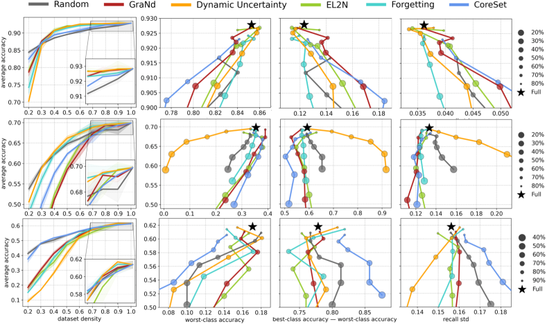
Figure 1: The average test performance of various data pruning algorithms against dataset density (fraction of samples remaining after pruning) and measures of class-wise fairness. Top: VGG-16 on CIFAR-10, Center: VGG-19 on CIFAR-100, Bottom: ResNet-18 on TinyImageNet. All results averaged over $3$ random seeds. Error bands represent min/max.

Fairness & Evaluation.

Fairness in machine learning concerns the issue of non-uniform accuracy over the data distribution (Caton and Haas, 2023). The majority of research focuses on group fairness where certain, often under-represented or sensitive, groups of the population enjoy worse predictive performance (Hashimoto et al., 2018; Thomas McCoy et al., 2020). In general, groups are subsets of classes, and worst-group accuracy is a standard optimization criterion in this domain (Sagawa* et al., 2020; Kirichenko et al., 2023; Rudner et al., 2024). The focus of this study is a special case of group fairness, classification bias, where groups are directly defined by class attributions. Classification bias commonly arises in the context of imbalanced datasets where tail classes require upsampling or importance weighting to produce models with strong worst-class performance (Cui et al., 2019; Barua et al., 2012; Tan et al., 2020; Chaudhuri et al., 2023). For balanced datasets, classification bias is found to be exacerbated by adversarial training (Li and Liu, 2023; Benz et al., 2021; Xu et al., 2021; Nanda et al., 2021; Ma et al., 2022) and network pruning (Paganini, 2020; Joseph et al., 2020; Tran et al., 2022; Good et al., 2022). These works measure classification bias in various ways ranging from visual inspection to confidence intervals for the slope of the linear regression that fits accuracy deviations around the mean across classes. Another common approach is to measure the class- or group-wise performance gaps relative to the baseline model (without adversarial training or pruning) (Hashemizadeh et al., 2023; Dai et al., 2023; Lin et al., 2022). However, this metric ignores the fact that this original model can be and often is highly unfair itself, and counts any potential improvement over it as unfavorable. Instead, we utilize a simpler and more natural suite of metrics to measure classification bias. Given accuracy (recall) $r_{k}$ for each class $k\in[K]$, we report (1) worst-class accuracy $\min_{k}r_{k}$, (2) difference between the maximum and the minimum recall $\max_{k}r_{k}$-$\min_{k}r_{k}$ (Joseph et al., 2020), and (3) standard deviation of recalls $\text{std}_{k}r_{k}$ (Ma et al., 2022).

Data Pruning Meets Fairness.

Although existing data pruning techniques have proven to achieve strong average generalization performance, no prior work systematically evaluated their robustness to classification bias. Among related works, Pote et al. (2023) studied how EL2N pruning affects the class-wise performance and found that, at high data density levels (e.g., $80$–$90\%$ remaining data), under-performing classes improve their accuracy compared to training on the full dataset. Zayed et al. (2023) propose a modification of EL2N to achieve fairness across protected groups with two attributes (e.g., male and female) in datasets with counterfactual augmentation, which is a rather specific setting. In this study, we eliminate this blind spot in the data pruning literature and analyze the trade-off between the average performance and classification bias exhibited by some of the most common data pruning methods: EL2N and GraNd (Paul et al., 2021), Influence (Yang et al., 2023), Forgetting (Toneva et al., 2019), Dynamic Uncertainty (He et al., 2023), and CoreSet (Sener and Savarese, 2018). We present the experimental details and hyperparameters in Appendix A.

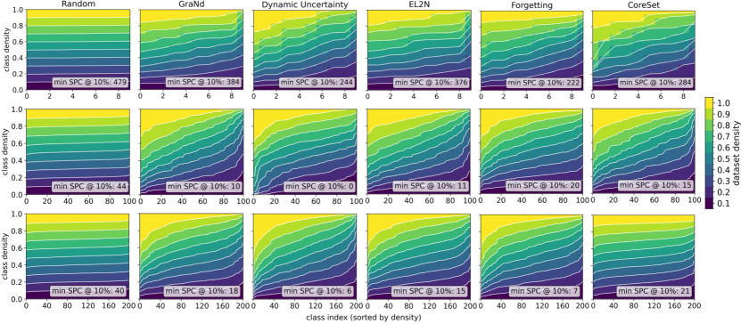
Figure 2: Sorted class densities in the training dataset pruned by various algorithms to different density levels. On each plot, we report the minimum number of samples per class (SPC) at $10\%$ dataset density. Top: VGG-16 on CIFAR-10, Center: VGG-19 on CIFAR-100, Bottom: ResNet-18 on TinyImageNet. Repeated over $3$ random seeds.

Data Pruning is Currently Unfair.

We conduct the first comprehensive comparative study of data pruning through the lens of class-wise fairness (Figure 1). First, we note that no pruning method is uniformly state-of-the-art, and the results vary considerably across model-dataset pairs. Among all algorithms, Dynamic Uncertainty with VGG-19 on CIFAR-100 presents a particularly interesting and instructive case. While it is arguably the best with respect to the average test performance, it fails miserably across all fairness metrics. Figure 2 reveals that it actually removes entire classes already at $10\%$ of CIFAR-100. Therefore, it seems plausible that Dynamic Uncertainty simply sacrifices the most difficult classes to retain strong performance on the easier ones. Figure 3 confirms our hypothesis: in contrast to other algorithms, at low density levels, Dynamic Uncertainty tends to prune classes with lower baseline accuracy (obtained from training on the full dataset) more aggressively, which entails a catastrophic classification bias hidden underneath a deceptively strong average accuracy. This observation presents a compelling argument for using criteria beyond average test performance for data pruning algorithms, particularly emphasizing classification bias.

Overall, existing algorithms exhibit poor robustness to bias, although several of them improve ever slightly over the full dataset. In particular, EL2N and GraNd achieve a relatively low classification bias, closely followed by Forgetting. At the same time, Forgetting has a substantially stronger average test accuracy compared to these three methods, falling short of Random only after pruning more than $60\%$ from CIFAR-100. Forgetting produces more balanced datasets than EL2N and GraNd at low densities (Figure 2), and tends to prune “easier” classes more aggressively compared to all other methods (Figure 3). These two properties seem to be beneficial, especially when the available training data is scarce.

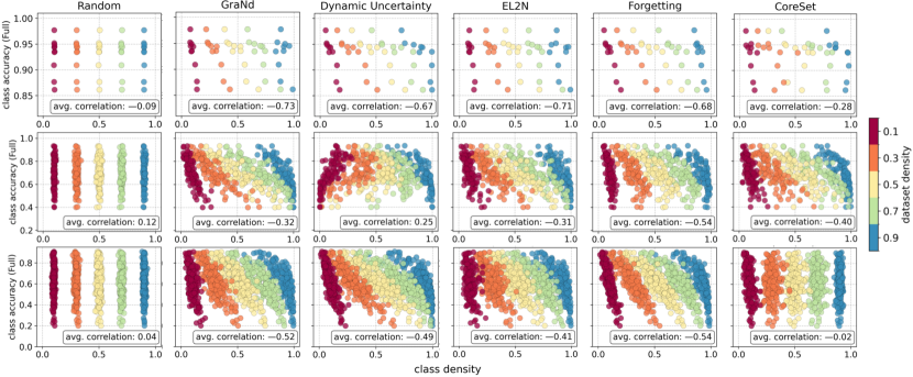
Figure 3: Full dataset test accuracy against density, across all classes, after pruning with different methods. We use the full dataset accuracy to capture the baseline “difficulty” of each class. On each plot, we report the correlation coefficient between these two quantities across classes, averaged over $5$ data density levels ($0.1$, $0.3$, $0.5$, $0.7$, $0.9$). Top: VGG-16 on CIFAR-10, Center: VGG-19 on CIFAR-100, Bottom: ResNet-18 on TinyImageNet. Experiments repeated over $3$ random seeds.

While the results in Figure 1 uncover strong classification bias, existing literature hints that data pruning should in fact be effective in mitigating the classification bias because it bears similarity to some fairness-driven optimization approaches. The majority of well-established and successful algorithms that optimize for worst-group performance apply importance weighting to effectively re-balance the long-tailed data distributions (cf. cost-sensitive learning (Elkan, 2001)). Taking this paradigm to an extreme, data pruning assigns zero weights to the pruned samples in the original dataset, trading some learning signal for faster convergence, and resource and memory efficiency. Furthermore, similarly to EL2N or Forgetting, the majority of cost-sensitive methods estimate class- or group-specific weights according to their difficulty. Thus, Sagawa* et al. (2020) optimize an approximate minimax DRO (distributionally robust) objective using a weighted sum of group-wise losses, putting higher mass on high-loss groups; Sinha et al. (2022) weigh samples by the current class-wise misclassification rates measured on a holdout validation set; Liu et al. (2021) pre-train a reference model to estimate the importance coefficients of groups for subsequent re-training. Similar cost-weighting strategies are adopted for robust knowledge distillation (Wang et al., 2023; Lukasik et al., 2022) and online batch selection (Kawaguchi and Lu, 2020; Mindermann et al., 2022). These techniques compute weights at the level of classes or sensitive groups and not for individual training samples. In the context of data pruning, this would correspond to selecting the appropriate density ratios across classes but subsampling randomly otherwise. While existing pruning algorithms automatically balance classes according to their validation errors fairly well (Figure 3), their overly scrupulous filtering within classes may be suboptimal. In support of this view, Ayed and Hayou (2023) formally show that integrating random sampling into score-based pruning procedures improves their average performance. In fact, random pruning is regarded as a notoriously strong baseline in active learning and data pruning (see Figure 1). In the next section, we propose and evaluate a random pruning algorithm that respects difficulty-based class-wise ratios.

3 Method & Results

We are ready to propose our “fairness-aware” data pruning method, which consists in random subsampling according to carefully selected target class-wise sizes. To imitate the behavior of the cost-sensitive learning procedures that optimize for worst-class accuracy as discussed in Section 2, we propose to select the pruning fraction of each class based on its validation performance given a preliminary model $\psi$ trained on the whole dataset. This query model is still required by all existing data pruning algorithms to compute scores, so we introduce no additional resource overhead.

Input: Target dataset density $d\in[0,1]$. For each class $k\in[K]$: $N_{k}$ samples in the original dataset and validation recall $r_{k}\in[0,1]$.

Initialize: Unsaturated set of classes $U\leftarrow[K]$, excess $E\leftarrow dN$, class densities $d_{k}\leftarrow 0\>\>\forall k\in[K]$.

while $E>0$ do

       $Z\leftarrow\frac{1}{E}\sum_{k\in U}N_{k}(1-r_{k})$;

       for $k\in U$ do

             $d^{\prime}_{k}\leftarrow(1-r_{k})/Z$;

             $d_{k}\leftarrow d_{k}+d^{\prime}_{k}$;

             $E\leftarrow E-N_{k}d^{\prime}_{k}$;

             if $d_{k}>1$ then

                  $U\leftarrow U\setminus\{k\}$;

                   $E\leftarrow E+N_{k}(d_{k}-1)$;

                  $d_{k}\leftarrow 1$

             end if

            

       end for

      

end while

Return : $\{d_{k}\}_{k=1}^{K}$.

Algorithm 1 MetriQ

Consider pruning a $K$-way classification dataset originally with $N$ samples down to density $0\leq d\leq 1$, so the target dataset size is $dN$ (prior literature sometimes refers to $1-d$ as the pruning fraction). Likewise, for each class $k\in[K]$, define $N_{k}$ to be the original number of samples so $N=\sum_{k=1}^{K}N_{k}$, and let $0<d_{k}\leq 1$ be the desired density of that class after pruning. Then, we set $d_{k}\propto 1-r_{k}$ where $r_{k}$ denotes recall (accuracy) of class $k$ computed by $\psi$ on a hold-out validation set. In particular, we define Metric-based Quotas (MetriQ) as $d_{k}=d(1-r_{k})/Z$ where $Z=\sum_{k=1}^{K}(1-r_{k})N_{k}\big{/}N$ is a normalizing factor to ensure that the target density is respected, i.e., $dN=\sum_{k=1}^{K}d_{k}N_{k}$. Alas, not all dataset densities $d\in[0,1]$ can be associated with a valid MetriQ collection; indeed, for large enough $d$, the required class proportions may demand $d_{k}>1$ for some $k\in[K]$. In such a case, we do not prune such classes and redistribute the excess density across unsaturated ($d_{k}<1$) classes according to their MetriQ proportions. The full procedure is described in Algorithm 1. This algorithm is guaranteed to terminate as the excess decreases in each iteration of the outer loop.

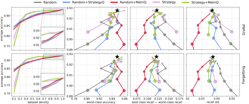
(a) VGG-16 on CIFAR-10

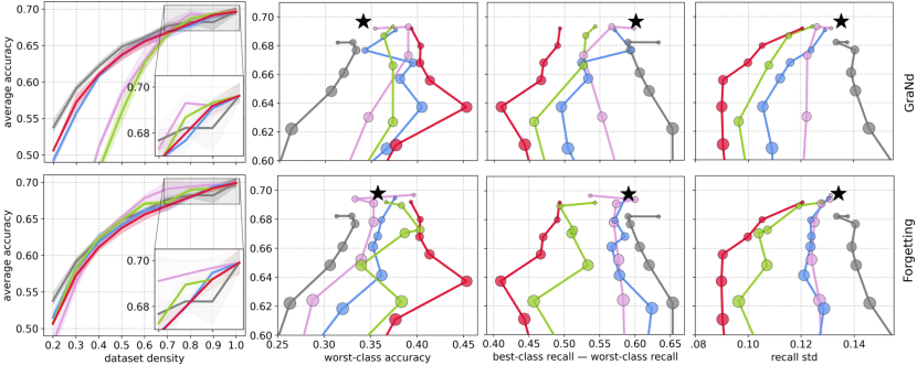
(b) VGG-19 on CIFAR-100

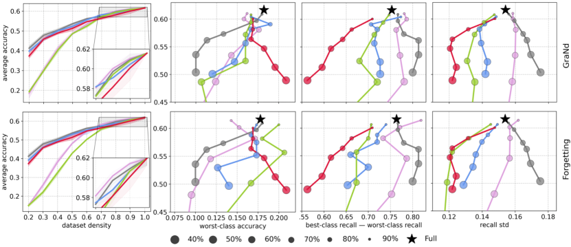
(c) ResNet-18 on TinyImageNet

Figure 4: The average test performance of various data pruning protocols against dataset density and measures of class-wise fairness. All results averaged over $3$ random seeds. Error bands represent min/max.

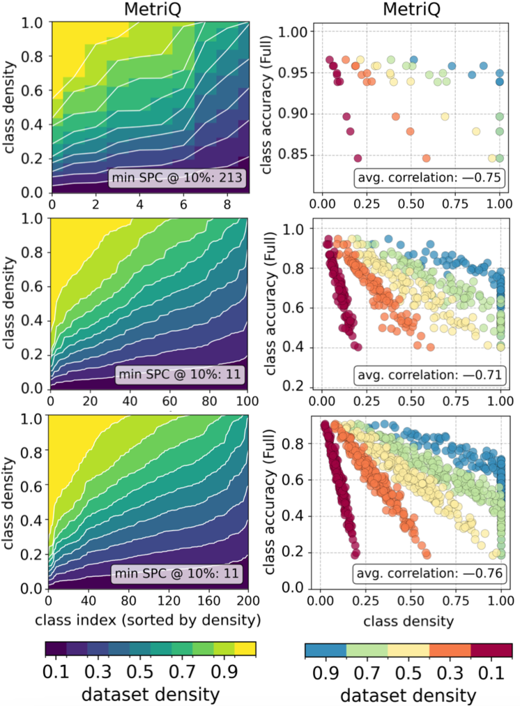
Figure 5: Class-wise densities (left) and full-dataset accuracies (right), cf. Figures 2 and 3. Top: VGG-16 on CIFAR-10, Middle: VGG-19 on CIFAR-100, Bottom: ResNet-18 on TinyImageNet.

Evaluation.

To validate the effectiveness of random pruning with MetriQ (Random+MetriQ) in reducing classification bias, we compare it to various baselines derived from two of the strongest pruning algorithms: GraNd (Paul et al., 2021), and Forgetting (Toneva et al., 2019). In addition to plain random pruning (Random)—removing a random subset of all training samples—for each of these two strategies, we consider (1) random pruning that respects class-wise ratios automatically determined by the strategy (Random+StrategyQ), (2) applying the strategy for pruning within classes but distributing sample quotas across classes according to MetriQ (Strategy+MetriQ), and (3) the strategy itself. The implementation details and hyperparameter choices are documented in Appendix A.

Results.

Figure 4 presents our results for (a) VGG-16 on CIFAR-10, (b) VGG-19 on CIFAR-100, and (c) ResNet-18 on TinyImageNet. Overall, MetriQ with random pruning consistently exhibits a significant improvement in distributional robustness of the trained models. In contrast to all other baselines that arguably achieve their highest worst-class accuracy at high dataset densities ($80$–$90\%$), our method reduces classification bias induced by the datasets as pruning continues, e.g., up to $30$–$40\%$ dataset density of TinyImageNet. Notably, Random+MetriQ improves all fairnes metrics compared to the full dataset on all model-dataset pairs, offering both robustness and data efficiency at the same time. For example, when pruning half of CIFAR-100, we achieve an increase in the worst-class accuracy of VGG-19 from $35.8\%$ to $45.4\%$—an almost $10\%$ change at a price of under $6\%$ of the average performance. The leftmost plots in Figure 4 reveal that Random+MetriQ does suffer a slightly larger degradation of the average accuracy as dataset density decreases compared to global random pruning, which is unavoidable given the natural trade-off between robustness and average performance. Yet at these low densities, the average accuracy of our method exceeds that of all other pruning algorithms.

As demonstrated in Figure 5, MetriQ produces exceptionally imbalanced datasets unless the density $d$ is too low by heavily pruning easy classes while leaving the more difficult ones intact. As expected from its design, the negative correlation between the full-dataset accuracy and density of each class is much more pronounced for MetriQ compared to existing pruning methods (cf. Figure 3). Based on our examination of these methods in Section 2, we conjectured that these two properties are associated with smaller classification bias, which is well-supported by MetriQ. Not only does it achieve unparalleled performance with random pruning, but it also enhances fairness of GraNd and Forgetting: Strategy+MetriQ curves trace a much better trade-off between the average and worst-class accuracies than their original counterparts (Strategy). At the same time, Random+StrategyQ fares similarly well, surpassing the vanilla algorithms, too. This indicates that robustness is achieved not only from the appropriate class ratios but also from pruning randomly as opposed to cherry-picking difficult samples. We develop more analytical intuition about this phenomenon in Section 4.

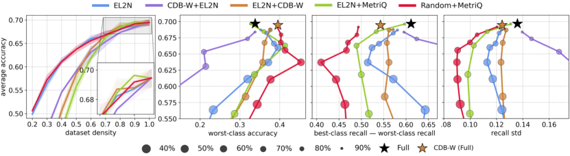
Figure 6: The average test performance of various data pruning protocols against dataset density and measures of class-wise fairness. VGG-19 on CIFAR-100. All results averaged over 3 random seeds. Error bands represent min/max.

A fairness baseline.

The results in Figure 4 provide solid evidence that Random+MetriQ is by far the state-of-the-art data pruning algorithm in the fairness framework. Not only is it superior to prior pruning baselines, it in fact produces significantly more robust models compared to the full dataset, too. Thus, we go further and test our method against one cost-sensitive learning technique, Class-wise Difficulty Based Weighted loss (CDB-W) (Sinha et al., 2022). In its simplest form adopted in this study, CDB-W dynamically updates class-specific weights $w_{k,t}=1-r_{k,t}$ at every epoch $t$ by computing recalls $r_{k,t}$ on a holdout validation set, which is precisely the proportions used by MetriQ. Throughout training, CDB-W uses these weights to upweigh the per-sample losses based on the corresponding class labels. As part of the evaluation, we test if the fairness-driven optimization of CDB-W can help data pruning (for these experiments, we use EL2N). To this end, we consider two scenarios: training the final model with CDB-W on the EL2N-pruned dataset (EL2N+CDB-W), and using a fair query model trained by CDB-W to generate EL2N scores (CDB-W+EL2N).

Having access to the full dataset, CDB-W improves the worst-class accuracy of VGG-19 on CIFAR-100 by $5.7\%$ compared to standard optimization, which is almost twice as short of the increase obtained by removing $50\%$ of the dataset with Random+MetriQ (Figure 4). When applied to EL2N-pruned datasets, CDB-W retains that original fairness level across sparsities, which is clearly inferior not only to Random+MetriQ but also to EL2N+MetriQ. Perhaps surprisingly, EL2N with scores computed by a query model trained with CDB-W fails spectacularly, inducing one of the worst bias observed in this study. Thus, MetriQ can compete with other existing methods that directly optimize for worst-class accuracy.

Imbalanced data.

In the literature, fairness issues almost exclusively arise in the context of long-tailed distributions where certain classes or groups appear far less often than others; for example, CDB-W was evaluated in this setting. While dataset imbalance may indeed exacerbate implicit bias of the trained models towards more prevalent classes, our study demonstrates that the key to robustness lies in the appropriate, difficulty-based class proportions rather than class balance per se. Even though the overall dataset size decreases, pruning with MetriQ can produce far more robust models compared to full but balanced datasets (Figure 5). Still, to promote consistency in evaluation and to further validate our algorithm, we consider long-tailed classification scenarios. We follow the approach used by Cui et al. (2019) to inject imbalance into the originally balanced TinyImageNet. In particular, we subsample each class $k\in[K]$ and retain $\mu^{k-1}$ of its original size; for an initially balanced dataset, the size ratio between the largest ($k=1$) and the smallest ($k=K$) classes becomes $\mu^{K-1}$, which is called the imbalance factor denoted by $I$. Figure 7 reveals that Random+MetriQ consistently beats EL2N in terms of both average and robust performance across a range of imbalance factors ($I=2,5,20$). Likewise, it almost always reduces bias of the unpruned imbalanced TinyImageNet even when training with a fairness-aware CDB-W procedure.

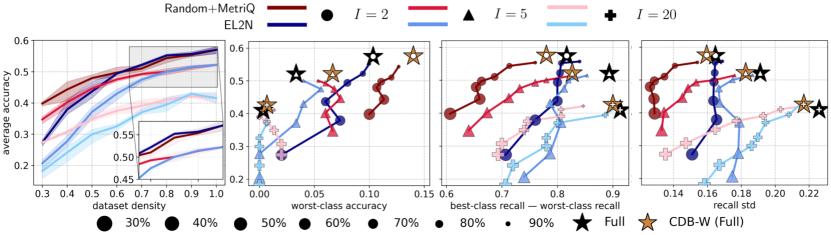
Figure 7: The average test performance of Random+MetriQ (red-toned curves) and EL2N (blue-toned curves) against dataset density and measures of class-wise fairness across dataset imbalance factors $I=2,5,20$. ResNet-18 on imbalanced TinyImageNet. All results averaged over 3 random seeds. Error bands represent min/max.

4 Theoretical Analysis

In this section, we derive analytical results for data pruning in a toy model of binary classification for a mixture of two univariate Gaussians with linear classifiers. Perhaps surprisingly, in this framework we can derive optimal fair class-wise densities that motivate our method, as well as demonstrate how prototypical pruning algorithms fail with respect to worst-class accuracy.

Let $\mathcal{M}$ be a mixture of two univariate Gaussians with conditional density functions $p(x|y=0)=\mathcal{N}(\mu_{0},\sigma_{0}^{2})$ and $p(x|y=1)=\mathcal{N}(\mu_{1},\sigma_{1}^{2})$, priors $\phi_{0}=\mathbb{P}(y=0)$ and $\phi_{1}=\mathbb{P}(y=1)$ ($\phi_{0}+\phi_{1}=1$), and $\sigma_{0}<\sigma_{1}$. Without loss of generality, we assume $\mu_{0}<\mu_{1}$. Consider linear decision rules $t\in\mathbb{R}\cup\{\pm\infty\}$ with a prediction function $\hat{y}_{t}(x)=\mathbf{1}\{x>t\}.$ The statistical 0-1 risks of the two classes are

$$R_{0}(t)=\Phi\left(\frac{\mu_{0}-t}{\sigma_{0}}\right),\qquad R_{1}(t)=\Phi\left(\frac{t-\mu_{1}}{\sigma_{1}}\right),$$ (1)

where $\Phi$ is the standard normal cumulative distribution function. Under some reasonable but nuanced conditions on the means, variances, and priors discussed in Appendix B.1, the optimal decision rule minimizing the average risk

$$R(t)=\phi_{0}R_{0}(t)+\phi_{1}R_{1}(t)$$ (2)

is computed by taking the larger of the two solutions to a quadratic equation $\partial R/\partial t=0$, which we denote by

$$t^{*}\left(\frac{\phi_{0}}{\phi_{1}}\right)=\frac{\mu_{0}\sigma^{2}_{1}-\mu_{1}\sigma^{2}_{0}+\sigma_{0}\sigma_{1}\sqrt{(\mu_{0}-\mu_{1})^{2}-2(\sigma^{2}_{0}-\sigma^{2}_{1})\log\frac{\phi_{0}\sigma_{1}}{\phi_{1}\sigma_{0}}}}{\sigma^{2}_{1}-\sigma^{2}_{0}}.$$ (3)

Note that $t^{*}(\phi_{0}/\phi_{1})$ is the rightmost intersection point of $\phi_{0}f_{0}(t)$ and $\phi_{1}f_{1}(t)$ where $f_{0}$ and $f_{1}$ are the corresponding probability density functions (Cavalli, 1945). Note that in the balanced case ($\phi_{0}=\phi_{1}$) the heavier-tailed class is more difficult and $R_{1}[t^{*}(1)]>R_{0}[t^{*}(1)]$.

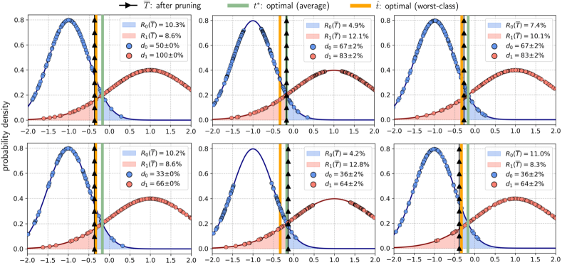
Figure 8: The effect of different pruning procedures on the solution to the binary classification with the mixture of Gaussians $\mathcal{M}$ defined by $\mu_{0}=-1$, $\mu_{1}=1$, $\sigma_{0}=0.5$, $\sigma_{1}=1$, and $\phi_{0}=\phi_{1}$. Pruning to density $75\%$ (top) and $50\%$ (bottom). Left: Random pruning with the optimal class-wise densities that satisfy $d_{1}\phi_{1}\sigma_{0}=d_{0}\phi_{0}\sigma_{1}$. Middle: SSP. Right: Random pruning with respect to class ratios provided by the SSP algorithm. The overall density of the dataset is $75\%$ (top row) and $50\%$ (bottom row). All results averaged across $10$ datasets $\{D_{i}\}_{i=1}^{10}$ each with $400$ points. The average ERM is $\overline{T}=\frac{1}{10}\sum_{i=1}^{10}T(D^{\prime}_{i})$ fitted to pruned datasets $D^{\prime}_{i}$. The class risks of the average and worst-class optimal decisions for this Gaussian mixture are $R_{0}[t^{*}(1)]=4.8\%$, $R_{1}[t^{*}(1)]=12.1\%$, and $R_{0}(\hat{t})=R_{1}(\hat{t})=9.1\%$.

We now turn to the standard (class-) distributionally robust objective: minimizing worst-class statistical risk gives rise to the decision threshold denoted by $\hat{t}=\text{argmin}_{t}\max\{R_{0}(t),R_{1}(t)\}$. As we show in Appendix B.2, $\hat{t}$ satisfies $R_{0}(\hat{t})=R_{1}(\hat{t})$, and Equation 1 then immediately yields

$$\hat{t}=(\mu_{0}\sigma_{1}+\mu_{1}\sigma_{0})/(\sigma_{0}+\sigma_{1}).$$ (4)

Note that $\hat{t}<t^{*}(1)$. This means that in the balanced case $\hat{t}$ is closer to $\mu_{0}$, the mean of the “easier” class. To understand how we should prune to achieve optimal worst-class accuracy, we compute class priors $\phi_{0}$ and $\phi_{1}$ that guarantee that the average risk minimization (Equation 2) achieves the best worst-class risk. These priors can be seen as the optimal class proportions in a “fairness-aware” dataset. Observe that, from Equation 3, $t^{*}(\sigma_{0}/\sigma_{1})=\hat{t}$ because the logarithm in the discriminant vanishes and we obtain Equation 4. Therefore, the optimal average risk minimizer coincides with the solution to the worst-case error over classes, and is achieved when the class priors $\phi_{0},\phi_{1}$ satisfy

$$\phi_{0}/\phi_{1}=\sigma_{0}/\sigma_{1}.$$ (5)

Intuitively, sufficiently large datasets sampled from $\mathcal{M}$ with class-conditionally independent samples mixed in proportions $N_{0}$ and $N_{1}$ should have their empirical 0-1 risk minimizers close to $t^{*}(N_{0}/N_{1})$. That is, randomly subsampling each class $k=0,1$ to densities $d_{k}$ that satisfy $d_{0}N_{0}\sigma_{1}=d_{1}N_{1}\sigma_{0}$ (see Equation 5) yields robust solutions with equal statistical risk across classes and, hence, optimal worst-class error. Figure 8 (left) confirms our analysis: the average empirical risk minimizer (ERM) $\overline{T}$ fitted to datasets pruned in this fashion lands near $\hat{t}$.

The class-conditional independence assumption we made above is crucial. While it is respected when subsampling randomly within each class, it clearly does not hold for existing, more sophisticated, data pruning algorithms. Therefore, even though they tend to prune easier classes more aggressively as evident from Figure 3, they rarely enjoy any improvement of the worst-class performance compared to the original dataset. We further illustrate this observation by replicating a supervised variant of the Self-Supervised Pruning (SSP) developed by Sorscher et al. (2022) for ImageNet. In this algorithm, we remove samples globally (i.e., irrespective of their class membership) located within a certain margin $M>0$ of their class means. Intuitively, this algorithm discards the easiest or the most representative samples from the most densely populated regions of the distribution. As illustrated in Figure 8 (middle), this method fortuitously prunes the easier class more aggressively; indeed, the amount of samples removed from a class with mean $\mu$ and variance $\sigma^{2}$ is proportional to the area under the probability density function over the pruning interval $[\mu-M,\mu+M]$, which is larger for smaller values of $\sigma$. Nevertheless, if the original dataset has classes mixed in proportions $N_{0}$ and $N_{1}$, the solution remains close to $t^{*}(N_{0}/N_{1})$ even after pruning, as we show formally in Appendix B.3. On the other hand, random subsampling according to class-wise pruning proportions defined by SSP does improve the worst-class accuracy, as illustrated in the right plots of Figure 8. This corresponds to our observation in Figure 4 that random pruning respecting the class proportions discovered by GraNd and Forgetting often improves fairness compared to these methods themselves.

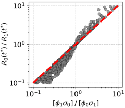
(a)

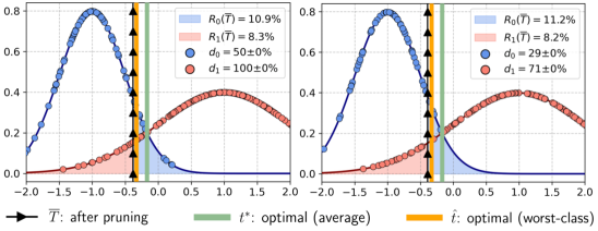
(b)

Figure 9: (a): Class-wise risk ratios of the optimal solution $t^{*}=t^{*}(\phi_{0}/\phi_{1})$ (MetriQ) vs. optimal ratios based on Equation 5 computed for various $\sigma_{0}$<$\sigma_{1}$ drawn uniformly from $[10^{-2},10^{2}]$ and $\phi_{0}\sim U[0,1]$ and $\phi_{1}=1-\phi_{0}$. The results are independent of $\mu_{0},\mu_{1}$. (b): Random pruning with MetriQ. Left: $d=75\%$; Right: $d=50\%$.

A priori, it is unclear how exactly the variance-based worst-case optimal pruning quotas in Equation 5 generalize to deep learning, and in particular how they can motivate error-based MetriQ, as proposed in Section 3. One could connect our theory to the feature distribution in the penultimate layer of neural networks and determine class densities from cluster variances around class means. In fact, SSP (Sorscher et al., 2022) uses such metrics to determine pruning scores for sample, using a pretrained model. However, such variances are noisy, especially for smaller class sizes, and hard to connect to class accuracies. Therefore, instead, we examine MetriQ in our toy framework. As argued above, given a dataset with class priors $N_{0}$ and $N_{1}$, the optimal class densities must satisfy $d_{0}N_{0}\sigma_{1}=d_{1}N_{1}\sigma_{0}$, while MetriQ requires $d_{0}R_{1}[t^{*}(N_{0}/N_{1})]=d_{1}R_{0}[t^{*}(N_{0}/N_{1})]$.

Figure 9a plots the two proportions for different Gaussian mixtures; we find that MetriQ approximates the optimal quotas quite well, especially when $\sigma_{1}/\sigma_{0}$ is small. Figure 9b demonstrates that random pruning according to MetriQ lands the average ERM near the optimal value. Thus, even though MetriQ does not enjoy simple theoretical guarantees, it still operates near-optimally in this toy setup.

5 Discussion

Data pruning—removal of uninformative samples from the training dataset—offers much needed efficiency in deep learning. However, all existing pruning algorithms are currently evaluated exclusively on their average performance, ignoring the potential impacts on fairness of the model predictions. Through a systematic study of the classification bias, we reveal that current methods often exacerbate the performance disparity across classes, which can deceptively co-occur with high average performance. At the same time, data pruning arguably operates in a similar manner to techniques that directly optimize for worst-class accuracy, suggesting that there is in fact much potential to improve model fairness by removing the right data. By examining elements of these algorithms, we find evidence that appropriately selecting the class-wise ratios but subsampling randomly within classes should reduce the implicit bias and produce more robust models. This leads us to formulate error-based class-wise pruning quotas coined MetriQ. At the same time, we find value in pruning randomly within classes, as opposed to cherry-picking, which is inherent to the existing data pruning techniques. We confirm the effectiveness of our method on a series of standard computer vision benchmarks; our simple pruning protocol traces the best trade-off between average and worst-class performance among all existing data pruning algorithms and related baselines. Additionally, we find theoretical justification for the phenomenal success of this simple strategy in a toy classification model.

Limitations & Future Work.

In this study, we focused our empirical evaluation exclusively on classification bias, so we only scratched the surface of fairness in deep learning. Further research is warranted to understand the effect of MetriQ and data pruning in general on worst-group accuracy and spurious correlations.

Appendix A Implementation Details

Our empirical work encompasses three standard computer vision benchmarks (Table 1). All code is implemented in PyTorch [Paszke et al., 2017] and run on an internal cluster equipped with NVIDIA RTX8000 GPUs. We make our code available at https://github.com/avysogorets/fair-data-pruning.

Data Pruning.

Data pruning methods require different procedures for training the query model and extracting scores for the training data. For EL2N and GraNd, we use $10\%$ of the full training length reported in Table 1 before calculating the importance scores, which is more than the minimum of $10$ epochs recommended by Paul et al. [2021]. To improve the score estimates, we repeat the procedure across $5$ random seeds and average the scores before pruning. Forgetting and Dynamic Uncertainty operate during training, so we execute a full optimization cycle of the query model but only do so once. Likewise, CoreSet is applied once on the fully trained embeddings. We use the greedy k-center variant of CoreSet. Since some of the methods require a hold-out validation set (e.g., MetriQ, CDB-W), we reserve $50\%$ of the test set for this purpose. This split is never used when reporting the final model performance.

Data Augmentation.

We employ data augmentation only when optimizing the final model. The same augmentation strategies are used for all three datasets. In particular, we normalize examples per-channel and randomly apply shifts by at most $4$ pixels in any direction and horizontal flips.

Model	Dataset	Epochs	Drop Epochs	Batch	LR	Decay
VGG-16	CIFAR-10	$160$	$80/120$	$128$	$0.1$	$1e$-$4$
VGG-19	CIFAR-100	$160$	$80/120$	$128$	$0.1$	$5e$-$4$
ResNet-18	TinyImageNet	$200$	$100/150$	$256$	$0.2$	$1e$-$4$

Table 1: Summary of experimental work and hyperparameters. All architectures include batch normalization [Ioffe and Szegedy, 2015] layers followed by ReLU activations. Models are initialized with Kaiming normal [He et al., 2015] and optimized by SGD (momentum $0.9$) with a stepwise LR schedule ($0.2\times$ drop factor applied on specified Drop Epochs) and categorical cross-entropy. The above hyperparameters are adopted from prior studies [Frankle et al., 2021, Wang et al., 2020].

Appendix B Theoretical Analysis for a Mixture of Gaussians

Consider the Gaussian mixture model and the hypothesis class of linear decision rules introduced in Section 4. Here we give a more formal treatment of the assumptions and claims made in that section.

B.1 Average risk minimization

Recall that we consider the average risk of the linear decision $\hat{y}_{t}(x)=\mathbf{1}\{x>t\}$ as $R(t)=\mathbb{E}_{x,y}[\ell(\hat{y}_{t}(x),y)]$, where the expectation is over $(x,y)\sim p(x,y)$ and class-conditional risk as $R_{y}(t)=\mathbb{E}_{x|y}[\ell(\hat{y}_{t}(x)),y)]$, where the expectation is over $x\sim p(x|y)$ for $y\in\{0,1\}$. If $\ell$ is the 0-1 loss, we thus obtain Equations 1 and 2. Recall that we have assumed $\sigma_{0}<\sigma_{1}$ and $\mu_{0}<\mu_{1}$.

We now give the precise conditions under which the average risk minimizer takes the form of $t^{*}(\phi_{0}/\phi_{1})$ from Equation 3—the larger intersection point between the graphs of scaled probability density functions $\phi_{0}f_{0}(t)$ and $\phi_{1}f_{1}(t)$.

First, we make an assumption that this intersection exists, i.e., the expression under the square root in Equation 3 is non-negative. That is, we require

$$\frac{\phi_{0}}{\phi_{1}}\geq\frac{\sigma_{0}}{\sigma_{1}}\text{exp}\left[-\frac{1}{2}\frac{(\mu_{0}-\mu_{1})^{2}}{\sigma^{2}_{1}-\sigma^{2}_{0}}\right].$$ (6)

This assumption simply guarantees the existence of intersection points of the two scaled density functions; provided this holds, we establish an additional condition on priors necessary for $t^{*}(\phi_{0}/\phi_{1})$ to be the average risk minimizer.

Theorem B.1.

If Equation 6 holds, define $t^{*}(\phi_{0}/\phi_{1})$ as in Equation 3. Then, $t^{*}(\phi_{0}/\phi_{1})$ is the statistical risk minimizer for the Gaussian mixture model if

$$\frac{\phi_{0}}{\phi_{1}}>\Phi\left(\frac{t^{*}(\phi_{0}/\phi_{1})-\mu_{1}}{\sigma_{1}}\right)\Bigg{/}\Phi\left(\frac{t^{*}(\phi_{0}/\phi_{1})-\mu_{0}}{\sigma_{0}}\right).$$ (7)

Proof.

For a decision rule $t\in\mathbb{R}\cup\{\pm\infty\}$, the statistical risk in the given Gaussian mixture model is given in Equation 1. The global minimum is achieved either at $\pm\infty$ or on $\mathbb{R}$. In the latter case, the minimizer is a solution to $\partial R(t)/\partial t=0$:

$$0=\frac{\partial R(t)}{\partial t} =-\frac{\phi_{0}}{\sqrt{2\pi}\sigma_{0}}\text{exp}\left[-\frac{1}{2}\left(\frac{\mu_{0}-t}{\sigma_{0}}\right)^{2}\right]+\frac{\phi_{1}}{\sqrt{2\pi}\sigma_{1}}\text{exp}\left[-\frac{1}{2}\left(\frac{t-\mu_{1}}{\sigma_{1}}\right)^{2}\right].$$

Rearranging and taking the logarithm on both sides yields

$$0=-2\log\left[\frac{\phi_{0}\sigma_{1}}{\phi_{1}\sigma_{0}}\right]-\left(\frac{t-\mu_{1}}{\sigma_{1}}\right)^{2}+\left(\frac{\mu_{0}-t}{\sigma_{0}}\right)^{2},$$ (8)

which is a quadratic equation in $t$ with solutions

$$t_{\pm}=\frac{\mu_{0}\sigma^{2}_{1}-\mu_{1}\sigma^{2}_{0}\pm\sigma_{0}\sigma_{1}\sqrt{(\mu_{0}-\mu_{1})^{2}+2(\sigma^{2}_{1}-\sigma^{2}_{0})\log\frac{\phi_{0}\sigma_{1}}{\phi_{1}\sigma_{0}}}}{\sigma^{2}_{1}-\sigma^{2}_{0}}.$$ (9)

By repeating the same steps for an inequality rather than equality, we conclude that $0<\partial R(t)/\partial t$ if and only if

$$0<-2\log\left[\frac{\phi_{0}\sigma_{1}}{\phi_{1}\sigma_{0}}\right]-\left(\frac{t-\mu_{1}}{\sigma_{1}}\right)^{2}+\left(\frac{\mu_{0}-t}{\sigma_{0}}\right)^{2}$$ (10)

similarly to Equation 8. This identity holds because the logarithm is a monotonically increasing function, preserving the inequality. Further expanding the right-hand side of Equation 10 and collecting similar terms, we arrive at a quadratic equation in $t$ with the leading (quadratic) coefficient $\sigma_{0}^{-2}-\sigma_{1}^{-2}>0$. Hence, the right-hand side defines an upward-branching parabola with zeros given in Equation 9 when they exist (we assume they do owing to assumption in Equation 6). The derivative of the statistical risk is positive whenever the right-hand side of Equation 10 is, i.e., on intervals $(-\infty,t_{-})$ and $(t_{+},\infty)$. Hence, the risk $R(t)$ must be increasing on the interval $(-\infty,t_{-})$, and so $t_{-}$ can never be a global minimizer. Likewise, the risk is increasing on the interval $(t_{+},\infty)$, which rules out $\{+\infty\}$. Therefore, we just need to establish that $R(-\infty)\geq R(t_{+})$, which is equivalent to Equation 7 since $t^{*}(\phi_{0}/\phi_{1})=t_{+}$. ∎

Remark.

We have considered unequal variances $\sigma_{0}^{2}<\sigma_{1}^{2}$ as a natural way to model classes with different difficulty. Yet note that our analysis still holds with slight modifications when $\sigma_{0}=\sigma_{1}=\sigma$. The difference in this case is that for any choice of priors, there is exactly one solution to Equation 8 (and exactly one intersection point of the scaled density functions), given by

$$t^{*}(\phi_{0}/\phi_{1})=\frac{2\sigma^{2}\log\left[\frac{\phi_{0}}{\phi_{1}}\right]+(\mu_{1}^{2}-\mu_{0}^{2})}{2(\mu_{1}-\mu_{0})}.$$

In particular, no additional assumptions as in Equation 6 to guarantee the existence of an intersection point need to be made. Furthermore, a similar derivative analysis as above implies that the risk is decreasing on the interval $(-\infty,t^{*}(\phi_{0}/\phi_{1}))$ and increasing on the interval $(t^{*}(\phi_{0}/\phi_{1}),+\infty)$, so that $t^{*}(\phi_{0}/\phi_{1})$ must be the statistical risk minimizer and the assumption in Equation 7 is, in fact, always satisfied. With these simplifications, the rest of the analysis presented in this section and in Section 4 holds for $\sigma_{0}=\sigma_{1}$.

B.2 Worst-class optimal priors

We wish to formally establish when $t^{*}(\sigma_{0}/\sigma_{1})$ as defined in Equation 4 minimizes both the average and worst-class risks when $\phi_{0}\propto\sigma_{0}$ and $\phi_{1}\propto\sigma_{1}$. For the first part, as we argued in Section B.1, these priors must satisfy the assumption in Equation 7 (Equation 6 is trivially satisfied). In this case, we can equivalently rewrite it as

$$\frac{\sigma_{0}}{\sigma_{1}} >\Phi\left(\frac{\mu_{0}\sigma_{1}+\mu_{1}\sigma_{0}-\mu_{1}\sigma_{0}-\mu_{1}\sigma_{1}}{\sigma_{1}(\sigma_{0}+\sigma_{1})}\right)\Bigg{/}\Phi\left(\frac{\mu_{0}\sigma_{1}+\mu_{1}\sigma_{0}-\mu_{0}\sigma_{0}-\mu_{0}\sigma_{1}}{\sigma_{1}(\sigma_{0}+\sigma_{1})}\right)$$

$$=\Phi\left(\frac{\mu_{0}-\mu_{1}}{\sigma_{0}+\sigma_{1}}\right)\Bigg{/}\Phi\left(\frac{\mu_{1}-\mu_{0}}{\sigma_{0}+\sigma_{1}}\right)=\left[1-\Phi\left(\frac{\mu_{1}-\mu_{0}}{\sigma_{0}+\sigma_{1}}\right)\right]\Bigg{/}\Phi\left(\frac{\mu_{1}-\mu_{0}}{\sigma_{0}+\sigma_{1}}\right),$$

Defining $z=\Phi\left(\frac{\mu_{1}-\mu_{0}}{\sigma_{0}+\sigma_{1}}\right)$, we arrive at $\sigma_{0}z>\sigma_{1}(1-z)$. By rearranging and collecting similar terms, we get $z>\frac{\sigma_{1}}{\sigma_{0}+\sigma_{1}}$, which is equivalent to

$$\mu_{1}-\mu_{0}>(\sigma_{0}+\sigma_{1})\Phi^{-1}\left(\frac{\sigma_{1}}{\sigma_{0}+\sigma_{1}}\right)$$ (11)

since $\Phi^{-1}$ is monotonically increasing. Hence, the assumption in Equation 7 can be interpreted as a lower bound on the separation between the two means $\mu_{0}$ and $\mu_{1}$. When this condition holds, $t^{*}(\sigma_{0}/\sigma_{1})$ minimizes the average statistical risk, as desired.

For the second part, we start by proving the following lemma.

Lemma B.2.

Suppose $f:\mathbb{R}\rightarrow[0,1]$ is a strictly increasing continuous function and $g:\mathbb{R}\rightarrow[0,1]$ is a strictly decreasing continuous function, satisfying

$$\begin{cases}\lim_{x\rightarrow-\infty}f(x)=\lim_{x\rightarrow+\infty}g(x)=0\\ \lim_{x\rightarrow+\infty}f(x)=\lim_{x\rightarrow-\infty}g(x)=1\end{cases}$$ (12)

The solution $x^{*}$ to $\min_{x}\max\{f(x),g(x)\}$ is unique and satisfies $f(x^{*})=g(x^{*})$.

Proof.

Define $h(x)=f(x)-g(x)$. Observe that $h(x)$ is a strictly increasing continuous function as $f$ and $-g$ are strictly increasing. Also, $\lim_{x\rightarrow-\infty}h(x)=-1$ and $\lim_{x\rightarrow\infty}h(x)=1$. From the Intermediate Value Theorem, there exists a point $x^{*}$, where $h(x^{*})=0$, i.e., $f(x^{*})=g(x^{*})$. Observe that $x<x^{*}$ implies $\max_{x}\{f(x),g(x)\}=g(x)$ and $x\geq x^{*}$ implies $\max_{x}\{f(x),g(x)\}=f(x)$. Therefore, the objective function decreases up to $x^{*}$ and then increases. Hence, $x^{*}$ is the minimizer of the objective $\min_{x}\max\{f(x),g(x)\}$. ∎

Since $f(t)=R_{1}(t)$ and $g(t)=R_{0}(t)$ meet the conditions of Lemma B.2, the minimizer of the worst-class risk $\hat{t}$ satisfies $R_{0}(\hat{t})=R_{1}(\hat{t})$. Equating the risks in Equation 1 then immediately proves the formula for $\hat{t}$ (Equation 4). Finally, note that $t^{*}(\sigma_{0}/\sigma_{1})=\hat{t}$ because of the vanishing logarithm. Therefore, $t^{*}(\sigma_{0}/\sigma_{1})$ minimizes both the average and worst-class statistical risks for a mixture with priors $\phi_{0}=\frac{\sigma_{0}}{\sigma_{0}+\sigma_{1}}$ and $\phi_{1}=\frac{\sigma_{1}}{\sigma_{0}+\sigma_{1}}$ provided that Equation 11 (reformulated assumption in Equation 7 for the given choice of priors) holds.

Finally, note that if $\sigma_{0}=\sigma_{1}$, $\hat{t}=t^{*}(\phi_{0}/\phi_{1})=(\mu_{0}+\mu_{1})/2$ for the optimal priors $\phi_{0}=\phi_{1}$, as expected.

B.3 The Effect of SSP

Our setting allows us to adapt and analyze a state-of-the-art baseline pruning algorithm, Self-Supervised Pruning (SSP) [Sorscher et al., 2022]. Recall that, in Section 4, we adopted a variant of SSP that removes samples within a margin $M>0$ of their class means. SSP performs k-means clustering in the embedding space of an ImageNet pre-trained self-supervised model and defines the difficulty of each data point by the cosine distance to its nearest cluster centroid, or prototype. In the case of two 1D Gaussians, this score corresponds to measuring the distance to the closest mean.

We claimed and demonstrated in Figure 8 that the optimal risk minimizer remains around $t^{*}(\phi_{0}/\phi_{1})$ even after pruning. In this section, we make these claims more precise. To this end, note that, for a Gaussian variable with variance $\sigma^{2}$, the removed probability mass is

$$\Phi\left(\frac{M+\mu-\mu}{\sigma}\right)-\Phi\left(\frac{\mu-(\mu-M)}{\sigma}\right)=2\Phi\left(\frac{M}{\sigma}\right)-1.$$ (13)

Now, for sufficiently small $M$, we can assume that the average risk minimizer lies within the interval $(\mu_{0}+M,\mu_{1}-M)$ (recall that the average risk minimizer of the original mixture lies between $\mu_{0}$ and $\mu_{1}$ owing to the assumption in Equation 7). In this case, the right tail of the easier class and the left tail of the more difficult class (these tails are misclassified for the two classes) are unaffected by pruning and, hence, the average risk after SSP $R^{\prime}(t)$ should remain proportional to the original risk $R(t)$. More formally, consider the class-wise risks after SSP:

$$R^{\prime}_{0}(t) =\frac{\Phi\left(\frac{\mu_{0}-t}{\sigma_{0}}\right)}{2-2\Phi\left(M/\sigma_{0}\right)}=\frac{R_{0}(t)}{2-2\Phi\left(M/\sigma_{0}\right)},$$

$$R^{\prime}_{1}(t) =\frac{\Phi\left(\frac{t-\mu_{1}}{\sigma_{1}}\right)}{2-2\Phi\left(M/\sigma_{1}\right)}=\frac{R_{1}(t)}{2-2\Phi\left(M/\sigma_{1}\right)}.$$

where the denominators are the normalizing factors based on Equation 13. To compute the average risk $R^{\prime}(t)=\phi_{0}^{\prime}R^{\prime}_{0}(t)+\phi_{1}^{\prime}R^{\prime}_{1}(t)$, we shall identify the modified class priors $\phi^{\prime}_{0}$ and $\phi^{\prime}_{1}$ after pruning. Again, from Equation 13, we obtain

$$\phi_{0}^{\prime} \equiv\phi_{0}\left[2-2\Phi\left(\frac{M}{\sigma_{0}}\right)\right],\qquad\phi_{1}^{\prime}\equiv\phi_{1}\left[2-2\Phi\left(\frac{M}{\sigma_{1}}\right)\right]$$ (14)

up to a global normalizing constant that ensures $\phi^{\prime}_{0}+\phi^{\prime}_{1}=1$. Therefore, the average risk is indeed proportional to $\phi_{0}R_{0}(t)+\phi_{1}R_{1}(t)=R(t)$, as desired, so the average risk minimizer after pruning coincides with the original one.

B.4 Multivariate Isotropic Gaussians

While the analysis of general multivariate Gaussians is beyond the scope of this paper, we show here that in the case of two isotropic multivariate Gaussians (i.e., $\text{Var}(x|y)=\sigma^{2}_{y}I$ for $y=0,1$), the arguments in Sections B.1–B.3 apply. In particular, we demonstrate that this scenario reduces to a univariate case.

For simplicity, assume that the means of the two Gaussians are located at $-\mu$ and $\mu$ for some $\mu\in\mathbb{R}^{d}$ for classes $y=0$ and $y=1$, respectively, which can always be achieved by a distance-preserving transformation (translation and/or rotation). Generalizing the linear classifier from Section 4, we now consider a hyperplane defined by a vector $w\in\mathbb{R}^{d}$ of unit $\ell_{2}$-norm and a threshold $t\in\mathbb{R}\cup\{\pm\infty\}$, classifying a point $x\in\mathbb{R}^{d}$ as $\mathbf{1}\{w^{\top}x\leq t\}$. Note that for a fixed vector $w\in\mathbb{R}^{d}$ and $x\sim\mathcal{N}(\mu,\sigma^{2}I_{d})$, we have $(w^{\top}x-w^{\top}\mu)/\sigma\sim\mathcal{N}(0,1)$ as a linear transformation of the isotropic Gaussian. We can now compute the class risks as

$$R_{1}(w,t) =P(w^{\top}x\leq t|y=1)$$

$$=P\left(\frac{w^{\top}x-w^{\top}\mu}{\sigma_{1}}\leq\frac{t-w^{\top}\mu}{\sigma_{1}}\bigg{|}y=1\right)=\Phi\left(\frac{t-w^{\top}\mu}{\sigma_{1}}\right),$$

$$R_{0}(w,t) =P(w^{\top}x\geq t|y=0)$$

$$=P\left(\frac{w^{\top}x+w^{\top}\mu}{\sigma_{0}}\geq\frac{t+w^{\top}\mu}{\sigma_{0}}\bigg{|}y=1\right)=\Phi\left(\frac{-t-w^{\top}\mu}{\sigma_{0}}\right).$$

The average risk given the class priors is thus

$$R(w,t)=\phi_{1}\Phi\left(\frac{t-w^{\top}\mu}{\sigma_{1}}\right)+\phi_{0}\Phi\left(\frac{-t-w^{\top}\mu}{\sigma_{0}}\right).$$

We will now show that for all the risk minimization problems we have considered in our theoretical analysis, we can equivalently minimize over a one-dimensional problem. It suffices to observe that for a fixed $t\in\mathbb{R}$, both $R_{0}(w,t)$ and $R_{1}(w,t)$ are minimized when $w$ (with $\|w\|_{2}=1$) coincides with $\mu/\|\mu\|$ because of monotonicity of $\Phi$. This leads to the expressions in Equation 1 with $\mu_{1,0}=\pm\mu/\|\mu\|$. Thus, to compute the minimum of $R(w,t)$ with respect to $w$ and $t$, we can equivalently minimize $R(\mu/\|\mu\|_{2},t)$ with respect to $t$. For the worst-class optimization

$$\min_{\|w\|=1,t}\max\{R_{1}(w,t),R_{0}(w,t)\}$$

observe that

$$\min_{t}\min_{\|w\|=1}\max\{R_{1}(w,t),R_{0}(w,t)\}=\min_{t}\max\{R_{1}(\mu/\|\mu\|,t),R_{0}(\mu/\|\mu\|,t)\}$$

Therefore, this problem also reduces to the minimization in the univariate case from Section B.2.

References

- Agarwal et al. [2020] Sharat Agarwal, Himanshu Arora, Saket Anand, and Chetan Arora. Contextual diversity for active learning. In Computer Vision–ECCV 2020: 16th European Conference, Glasgow, UK, August 23–28, 2020, Proceedings, Part XVI 16, pages 137–153. Springer, 2020.
- Ayed and Hayou [2023] Fadhel Ayed and Soufiane Hayou. Data pruning and neural scaling laws: fundamental limitations of score-based algorithms. Transactions on Machine Learning Research, 2023. ISSN 2835-8856.
- Barua et al. [2012] Sukarna Barua, Md Monirul Islam, Xin Yao, and Kazuyuki Murase. Mwmote–majority weighted minority oversampling technique for imbalanced data set learning. IEEE Transactions on knowledge and data engineering, 26(2):405–425, 2012.
- Beluch et al. [2018] William H Beluch, Tim Genewein, Andreas Nürnberger, and Jan M Köhler. The power of ensembles for active learning in image classification. In Proceedings of the IEEE Conference on Computer Vision and Pattern Recognition, pages 9368–9377, 2018.
- Benz et al. [2021] Philipp Benz, Chaoning Zhang, Adil Karjauv, and In So Kweon. Robustness may be at odds with fairness: An empirical study on class-wise accuracy. In NeurIPS 2020 Workshop on Pre-registration in Machine Learning, pages 325–342. PMLR, 2021.
- Caton and Haas [2023] Simon Caton and Christian Haas. Fairness in machine learning: A survey. ACM Comput. Surv., aug 2023.
- Cavalli [1945] Luigi Cavalli. Alcuni problemi della analisi biometrica di popolazioni naturali, 1945.
- Cazenavette et al. [2022] George Cazenavette, Tongzhou Wang, Antonio Torralba, Alexei A Efros, and Jun-Yan Zhu. Dataset distillation by matching training trajectories. In Proceedings of the IEEE/CVF Conference on Computer Vision and Pattern Recognition, pages 4750–4759, 2022.
- Chaudhuri et al. [2023] Kamalika Chaudhuri, Kartik Ahuja, Martin Arjovsky, and David Lopez-Paz. Why does throwing away data improve worst-group error? In Andreas Krause, Emma Brunskill, Kyunghyun Cho, Barbara Engelhardt, Sivan Sabato, and Jonathan Scarlett, editors, Proceedings of the 40th International Conference on Machine Learning, volume 202 of Proceedings of Machine Learning Research, pages 4144–4188. PMLR, 23–29 Jul 2023.
- Chawla et al. [2002] Nitesh V Chawla, Kevin W Bowyer, Lawrence O Hall, and W Philip Kegelmeyer. Smote: synthetic minority over-sampling technique. Journal of artificial intelligence research, 16:321–357, 2002.
- Chen et al. [2017] Robert S Chen, Brendan Lucier, Yaron Singer, and Vasilis Syrgkanis. Robust optimization for non-convex objectives. Advances in Neural Information Processing Systems, 30, 2017.
- Cui et al. [2019] Yin Cui, Menglin Jia, Tsung-Yi Lin, Yang Song, and Serge Belongie. Class-balanced loss based on effective number of samples. In Proceedings of the IEEE/CVF conference on computer vision and pattern recognition, pages 9268–9277, 2019.
- Dai et al. [2023] Yucong Dai, Gen Li, Feng Luo, Xiaolong Ma, and Yongkai Wu. Coupling fairness and pruning in a single run: a bi-level optimization perspective. arXiv preprint arXiv:2312.10181, 2023.
- Dwork et al. [2012] Cynthia Dwork, Moritz Hardt, Toniann Pitassi, Omer Reingold, and Richard Zemel. Fairness through awareness. In Proceedings of the 3rd innovations in theoretical computer science conference, pages 214–226, 2012.
- Elkan [2001] Charles Elkan. The foundations of cost-sensitive learning. In International joint conference on artificial intelligence, volume 17, pages 973–978. Lawrence Erlbaum Associates Ltd, 2001.
- Feldman [2020] Dan Feldman. Core-sets: An updated survey. WIREs Data Mining and Knowledge Discovery, 10(1):e1335, 2020.
- Feng et al. [2024] Yunzhen Feng, Shanmukha Ramakrishna Vedantam, and Julia Kempe. Embarrassingly simple dataset distillation. In The Twelfth International Conference on Learning Representations (ICLR), 2024.
- Frankle et al. [2021] Jonathan Frankle, Gintare Karolina Dziugaite, Daniel Roy, and Michael Carbin. Pruning neural networks at initialization: Why are we missing the mark? In International Conference on Learning Representations, 2021.
- Good et al. [2022] Aidan Good, Jiaqi Lin, Xin Yu, Hannah Sieg, Mikey Fergurson, Shandian Zhe, Jerzy Wieczorek, and Thiago Serra. Recall distortion in neural network pruning and the undecayed pruning algorithm. Advances in Neural Information Processing Systems, 35:32762–32776, 2022.
- Gordon et al. [2021] Mitchell A Gordon, Kevin Duh, and Jared Kaplan. Data and parameter scaling laws for neural machine translation. In Marie-Francine Moens, Xuanjing Huang, Lucia Specia, and Scott Wen-tau Yih, editors, Proceedings of the 2021 Conference on Empirical Methods in Natural Language Processing, pages 5915–5922, Online and Punta Cana, Dominican Republic, November 2021. Association for Computational Linguistics.
- Guo et al. [2022] Chengcheng Guo, Bo Zhao, and Yanbing Bai. Deepcore: A comprehensive library for coreset selection in deep learning. In International Conference on Database and Expert Systems Applications, pages 181–195. Springer, 2022.
- Hardt et al. [2016] Moritz Hardt, Eric Price, and Nati Srebro. Equality of opportunity in supervised learning. Advances in neural information processing systems, 29, 2016.
- Hashemizadeh et al. [2023] Meraj Hashemizadeh, Juan Ramirez, Rohan Sukumaran, Golnoosh Farnadi, Simon Lacoste-Julien, and Jose Gallego-Posada. Balancing act: Constraining disparate impact in sparse models, 2023.
- Hashimoto et al. [2018] Tatsunori Hashimoto, Megha Srivastava, Hongseok Namkoong, and Percy Liang. Fairness without demographics in repeated loss minimization. In International Conference on Machine Learning, pages 1929–1938. PMLR, 2018.
- He et al. [2015] Kaiming He, Xiangyu Zhang, Shaoqing Ren, and Jian Sun. Delving deep into rectifiers: Surpassing human-level performance on imagenet classification. In Proceedings of the IEEE international conference on computer vision, pages 1026–1034, 2015.
- He et al. [2023] Muyang He, Shuo Yang, Tiejun Huang, and Bo Zhao. Large-scale dataset pruning with dynamic uncertainty. arXiv preprint arXiv:2306.05175, 2023.
- Hestness et al. [2017] Joel Hestness, Sharan Narang, Newsha Ardalani, Gregory Diamos, Heewoo Jun, Hassan Kianinejad, Md Mostofa Ali Patwary, Yang Yang, and Yanqi Zhou. Deep learning scaling is predictable, empirically. arXiv preprint arXiv:1712.00409, 2017.
- Idrissi et al. [2022] Badr Youbi Idrissi, Martin Arjovsky, Mohammad Pezeshki, and David Lopez-Paz. Simple data balancing achieves competitive worst-group-accuracy. In Bernhard Schölkopf, Caroline Uhler, and Kun Zhang, editors, Proceedings of the First Conference on Causal Learning and Reasoning, volume 177 of Proceedings of Machine Learning Research, pages 336–351. PMLR, 11–13 Apr 2022.
- Ioffe and Szegedy [2015] Sergey Ioffe and Christian Szegedy. Batch normalization: Accelerating deep network training by reducing internal covariate shift. In Proceedings of the 32nd International Conference on International Conference on Machine Learning - Volume 37, ICML’15, page 448–456. JMLR.org, 2015.
- Joseph et al. [2020] Vinu Joseph, Shoaib Ahmed Siddiqui, Aditya Bhaskara, Ganesh Gopalakrishnan, Saurav Muralidharan, Michael Garland, Sheraz Ahmed, and Andreas Dengel. Going beyond classification accuracy metrics in model compression. arXiv preprint arXiv:2012.01604, 2020.
- Kaplan et al. [2020] Jared Kaplan, Sam McCandlish, Tom Henighan, Tom B. Brown, Benjamin Chess, Rewon Child, Scott Gray, Alec Radford, Jeffrey Wu, and Dario Amodei. Scaling laws for neural language models. arXiv preprint arXiv:2001.08361, 2020.
- Kawaguchi and Lu [2020] Kenji Kawaguchi and Haihao Lu. Ordered sgd: A new stochastic optimization framework for empirical risk minimization. In International Conference on Artificial Intelligence and Statistics, pages 669–679. PMLR, 2020.
- Kirichenko et al. [2023] Polina Kirichenko, Pavel Izmailov, and Andrew Gordon Wilson. Last layer re-training is sufficient for robustness to spurious correlations. In The Eleventh International Conference on Learning Representations, 2023.
- Kirsch et al. [2019] Andreas Kirsch, Joost Van Amersfoort, and Yarin Gal. Batchbald: Efficient and diverse batch acquisition for deep bayesian active learning. Advances in neural information processing systems, 32, 2019.
- Kwok et al. [2024] Devin Kwok, Nikhil Anand, Jonathan Frankle, Gintare Karolina Dziugaite, and David Rolnick. Dataset difficulty and the role of inductive bias. arXiv preprint arXiv:2401.01867, 2024.
- Li and Liu [2023] Boqi Li and Weiwei Liu. Wat: improve the worst-class robustness in adversarial training. AAAI’23/IAAI’23/EAAI’23. AAAI Press, 2023. ISBN 978-1-57735-880-0.
- Lin et al. [2022] Xiaofeng Lin, Seungbae Kim, and Jungseock Joo. Fairgrape: Fairness-aware gradient pruning method for face attribute classification. In Computer Vision – ECCV 2022: 17th European Conference, Tel Aviv, Israel, October 23–27, 2022, Proceedings, Part XIII, page 414–432, Berlin, Heidelberg, 2022. Springer-Verlag.
- Liu et al. [2021] Evan Z Liu, Behzad Haghgoo, Annie S Chen, Aditi Raghunathan, Pang Wei Koh, Shiori Sagawa, Percy Liang, and Chelsea Finn. Just train twice: Improving group robustness without training group information. In Marina Meila and Tong Zhang, editors, Proceedings of the 38th International Conference on Machine Learning, volume 139 of Proceedings of Machine Learning Research, pages 6781–6792. PMLR, 18–24 Jul 2021.
- Lukasik et al. [2022] Michal Lukasik, Srinadh Bhojanapalli, Aditya Krishna Menon, and Sanjiv Kumar. Teacher’s pet: understanding and mitigating biases in distillation. Transactions on Machine Learning Research, 2022. ISSN 2835-8856.
- Ma et al. [2022] Xinsong Ma, Zekai Wang, and Weiwei Liu. On the tradeoff between robustness and fairness. In Alice H. Oh, Alekh Agarwal, Danielle Belgrave, and Kyunghyun Cho, editors, Advances in Neural Information Processing Systems, 2022.
- Mindermann et al. [2022] Sören Mindermann, Jan M Brauner, Muhammed T Razzak, Mrinank Sharma, Andreas Kirsch, Winnie Xu, Benedikt Höltgen, Aidan N Gomez, Adrien Morisot, Sebastian Farquhar, et al. Prioritized training on points that are learnable, worth learning, and not yet learnt. In International Conference on Machine Learning, pages 15630–15649. PMLR, 2022.
- Mirzasoleiman et al. [2020] Baharan Mirzasoleiman, Jeff Bilmes, and Jure Leskovec. Coresets for data-efficient training of machine learning models. In International Conference on Machine Learning, pages 6950–6960. PMLR, 2020.
- Nanda et al. [2021] Vedant Nanda, Samuel Dooley, Sahil Singla, Soheil Feizi, and John P. Dickerson. Fairness through robustness: Investigating robustness disparity in deep learning. In Proceedings of the 2021 ACM Conference on Fairness, Accountability, and Transparency, FAccT ’21, page 466–477, New York, NY, USA, 2021. Association for Computing Machinery.
- Nguyen et al. [2021] Timothy Nguyen, Roman Novak, Lechao Xiao, and Jaehoon Lee. Dataset distillation with infinitely wide convolutional networks. In A. Beygelzimer, Y. Dauphin, P. Liang, and J. Wortman Vaughan, editors, Advances in Neural Information Processing Systems, 2021.
- Paganini [2020] Michela Paganini. Prune responsibly, 2020.
- Paszke et al. [2017] Adam Paszke, Sam Gross, Soumith Chintala, Gregory Chanan, Edward Yang, Zachary DeVito, Zeming Lin, Alban Desmaison, Luca Antiga, and Adam Lerer. Automatic differentiation in pytorch. 2017.
- Paul et al. [2021] Mansheej Paul, Surya Ganguli, and Gintare Karolina Dziugaite. Deep learning on a data diet: Finding important examples early in training. In A. Beygelzimer, Y. Dauphin, P. Liang, and J. Wortman Vaughan, editors, Advances in Neural Information Processing Systems, 2021.
- Pote et al. [2023] Tejas Pote, Mohammed Adnan, Yigit Yargic, and Yani Ioannou. Classification bias on a data diet. In Conference on Parsimony and Learning (Recent Spotlight Track), 2023.
- Ren et al. [2021] Pengzhen Ren, Yun Xiao, Xiaojun Chang, Po-Yao Huang, Zhihui Li, Brij B Gupta, Xiaojiang Chen, and Xin Wang. A survey of deep active learning. ACM computing surveys (CSUR), 54(9):1–40, 2021.
- Rosenfeld et al. [2020] Jonathan S. Rosenfeld, Amir Rosenfeld, Yonatan Belinkov, and Nir Shavit. A constructive prediction of the generalization error across scales. In International Conference on Learning Representations (ICLR) 2020, 2020.
- Rudner et al. [2024] Tim GJ Rudner, Ya Shi Zhang, Andrew Gordon Wilson, and Julia Kempe. Mind the gap: Improving robustness to subpopulation shifts with group-aware priors. In International Conference on Artificial Intelligence and Statistics (AISTATS), 2024.
- Sagawa* et al. [2020] Shiori Sagawa*, Pang Wei Koh*, Tatsunori B. Hashimoto, and Percy Liang. Distributionally robust neural networks. In International Conference on Learning Representations, 2020.
- Sener and Savarese [2018] Ozan Sener and Silvio Savarese. Active learning for convolutional neural networks: A core-set approach. In International Conference on Learning Representations, 2018.
- Sinha et al. [2022] Saptarshi Sinha, Hiroki Ohashi, and Katsuyuki Nakamura. Class-difficulty based methods for long-tailed visual recognition. International Journal of Computer Vision, 130(10):2517–2531, 2022.
- Sorscher et al. [2022] Ben Sorscher, Robert Geirhos, Shashank Shekhar, Surya Ganguli, and Ari S. Morcos. Beyond neural scaling laws: beating power law scaling via data pruning. In Alice H. Oh, Alekh Agarwal, Danielle Belgrave, and Kyunghyun Cho, editors, Advances in Neural Information Processing Systems, 2022.
- Such et al. [2020] Felipe Petroski Such, Aditya Rawal, Joel Lehman, Kenneth Stanley, and Jeffrey Clune. Generative teaching networks: Accelerating neural architecture search by learning to generate synthetic training data. In International Conference on Machine Learning, pages 9206–9216. PMLR, 2020.
- Sucholutsky and Schonlau [2021] Ilia Sucholutsky and Matthias Schonlau. Soft-label dataset distillation and text dataset distillation. In 2021 International Joint Conference on Neural Networks (IJCNN), pages 1–8. IEEE, 2021.
- Tan et al. [2020] Jingru Tan, Changbao Wang, Buyu Li, Quanquan Li, Wanli Ouyang, Changqing Yin, and Junjie Yan. Equalization loss for long-tailed object recognition. In Proceedings of the IEEE/CVF conference on computer vision and pattern recognition, pages 11662–11671, 2020.
- Tharwat and Schenck [2023] Alaa Tharwat and Wolfram Schenck. A survey on active learning: State-of-the-art, practical challenges and research directions. Mathematics, 11(4), 2023.
- Thomas McCoy et al. [2020] R. Thomas McCoy, Ellie Pavlick, and Tal Linzen. Right for the wrong reasons: Diagnosing syntactic heuristics in natural language inference. In ACL 2019 - 57th Annual Meeting of the Association for Computational Linguistics, Proceedings of the Conference, ACL 2019 - 57th Annual Meeting of the Association for Computational Linguistics, Proceedings of the Conference, pages 3428–3448. Association for Computational Linguistics (ACL), 2020.
- Toneva et al. [2019] Mariya Toneva, Alessandro Sordoni, Remi Tachet des Combes, Adam Trischler, Yoshua Bengio, and Geoffrey J. Gordon. An empirical study of example forgetting during deep neural network learning. In International Conference on Learning Representations, 2019.
- Tran et al. [2022] Cuong Tran, Ferdinando Fioretto, Jung-Eun Kim, and Rakshit Naidu. Pruning has a disparate impact on model accuracy. In Alice H. Oh, Alekh Agarwal, Danielle Belgrave, and Kyunghyun Cho, editors, Advances in Neural Information Processing Systems, 2022.
- Wang et al. [2020] Chaoqi Wang, Guodong Zhang, and Roger Grosse. Picking winning tickets before training by preserving gradient flow. In International Conference on Learning Representations, 2020.
- Wang et al. [2023] Serena Wang, Harikrishna Narasimhan, Yichen Zhou, Sara Hooker, Michal Lukasik, and Aditya Krishna Menon. Robust distillation for worst-class performance: on the interplay between teacher and student objectives. In Robin J. Evans and Ilya Shpitser, editors, Proceedings of the Thirty-Ninth Conference on Uncertainty in Artificial Intelligence, volume 216 of Proceedings of Machine Learning Research, pages 2237–2247. PMLR, 31 Jul–04 Aug 2023.
- Welling [2009] Max Welling. Herding dynamical weights to learn. In Proceedings of the 26th Annual International Conference on Machine Learning, ICML ’09, page 1121–1128, New York, NY, USA, 2009. Association for Computing Machinery.
- Xu et al. [2021] Han Xu, Xiaorui Liu, Yaxin Li, Anil Jain, and Jiliang Tang. To be robust or to be fair: Towards fairness in adversarial training. In International conference on machine learning, pages 11492–11501. PMLR, 2021.
- Yang et al. [2023] Shuo Yang, Zeke Xie, Hanyu Peng, Min Xu, Mingming Sun, and Ping Li. Dataset pruning: Reducing training data by examining generalization influence. In The Eleventh International Conference on Learning Representations, 2023.
- Zayed et al. [2023] Abdelrahman Zayed, Prasanna Parthasarathi, Gonçalo Mordido, Hamid Palangi, Samira Shabanian, and Sarath Chandar. Deep learning on a healthy data diet: finding important examples for fairness. In Proceedings of the Thirty-Seventh AAAI Conference on Artificial Intelligence and Thirty-Fifth Conference on Innovative Applications of Artificial Intelligence and Thirteenth Symposium on Educational Advances in Artificial Intelligence, AAAI’23/IAAI’23/EAAI’23. AAAI Press, 2023.
- Zhao and Bilen [2023] Bo Zhao and Hakan Bilen. Dataset condensation with distribution matching. In Proceedings of the IEEE/CVF Winter Conference on Applications of Computer Vision, pages 6514–6523, 2023.
- Zheng et al. [2023] Haizhong Zheng, Rui Liu, Fan Lai, and Atul Prakash. Coverage-centric coreset selection for high pruning rates. In The Eleventh International Conference on Learning Representations, 2023.