Maximum likelihood estimation in continuous affine Volterra processes in the ergodic regime

Abstract.

We study statistical inference of the drift parameters for the Volterra Ornstein-Uhlenbeck process on $\mathbb{R}$ and the Volterra Cox-Ingersoll-Ross process on $\mathbb{R}_{+}$ in the ergodic regime. For continuous-time observations, we derive the corresponding maximum likelihood estimators and show that they are strongly consistent and asymptotically normal locally uniformly in the parameters. For the case of discrete high-frequency observations, we prove similar results by discretization of the continuous-time maximum likelihood estimator. Finally, for discrete low-frequency observations, we show that the method of moments is consistent. Our proofs are crucially based on the law of large numbers. To prove the latter, we introduce the notion of asymptotic independence which has the advantage that it can be effectively verified by the affine transformation formula and convergence of the characteristic function. As a side product of our results, we show that the stationary processes are ergodic.

1. Introduction

1.1. Overview

Stochastic Volterra processes have gained increased attention e.g. due to their ability to capture the rough behaviour of sample paths (for an overview of the literature see e.g. [16]), and their flexibility to describe short and long-range dependencies [41]. In the absence of jumps and dimension one, a stochastic Volterra process (of convolution type) is given by

$$X_{t}=x_{0}+\int_{0}^{t}K(t-s)b(X_{s})ds+\int_{0}^{t}K(t-s)\sigma(X_{s})dB_{s},$$ (1.1)

where $(B_{t})_{t\geq 0}$ denotes a one-dimensional standard Brownian motion, $K\in L_{loc}^{2}(\mathbb{R}_{+})$ the Volterra kernel, and $b,\sigma:\mathbb{R}\longrightarrow\mathbb{R}$ are the drift and diffusion coefficients. The fractional Riemann-Liouville kernel

$$K_{\alpha}(t)=\frac{t^{\alpha-1}}{\Gamma(\alpha)},\qquad\alpha\in(1/2,1]$$ (1.2)

constitutes the most prominent example of Volterra kernels that allow for flexible incorporation of rough sample path behaviour. Other examples of Volterra kernels covered by this work are, e.g., the exponentially damped fractional kernel $K(t)=\frac{t^{\alpha-1}}{\Gamma(\alpha)}e^{-\lambda t}$, $K(t)=\sum_{j=1}^{N}c_{j}e^{-\lambda_{j}t}$ used for the Markovian approximation of solutions of (1.1) [1, 7], and the fractional $\log$-kernel $K(t)=\ln(1+t^{-\alpha})$ with $\alpha\in(0,1]$.

Processes of the form (1.1) provide a feasible framework for the modelling of rough volatility in Mathematical Finance, see e.g. [8, 18, 25, 26]. If the coefficients $b$ and $\sigma^{2}$ are affine linear in the state variable, then (1.1) is called affine Volterra process. In contrast to general stochastic Volterra processes, an important advantage of affine Volterra processes lies in their analytical traceability, see [17, 19]. For such processes, many computations can be carried out semi-explicit (e.g. via the affine transformation formula), making affine Volterra processes feasible for particular applications such as option pricing, see e.g. [2, 15, 19, 30]. For one-dimensional affine Volterra processes, the drift is necessarily given by

$$b(x)=b+\beta x$$ (1.3)

while for the diffusion coefficient, we consider the following two cases:

1. Volterra Ornstein-Uhlenbeck process on $\mathbb{R}$ where $\sigma(x)=\sigma$;

2. Volterra Cox-Ingersoll-Ross process on $\mathbb{R}_{+}$ where $\sigma(x)=\sigma\sqrt{x}$.

In this work, we study the maximum-likelihood estimation (MLE) of the drift parameters $(b,\beta)$. Analogous results for classical affine processes have been studied in [5, 6], while we refer to [34] for the general theory on statistical inference for Markov diffusion processes. For stochastic equations driven by the fractional Brownian motion, statistical inference is currently under active investigation [32, 39], see also [31, 33, 29] for the specific case of fractional Ornstein-Uhlenbeck process, and [38] for the case of the fractional square-root process. Although the models studied therein appear similar to models based on Volterra equations, there are a few important differences that make this work not a particular instance of the theory developed therein. Indeed, for Volterra processes the noise is defined in terms of a convolution with a usual Ito integral, while the integration theory for the fBm is e.g. based on Gaussian White noise calculus or for $H>1/2$ may also be defined in a pathwise sense. Moreover, for our setting, the Volterra kernel is also present in the drift and not only in the noise which requires additional care and more importantly leads to different ergodic behaviour, see [13]. Thus, based on the methods described below, this work complements the existing literature towards statistical inference for stochastic Volterra equations (1.1) applicable to a general class of completely monotone Volterra kernels $K$ beyond the fractional.

Finally, let us mention the recent PhD Thesis [43] where the estimation of $\beta$ (with $b=0$) for the Volterra Ornstein-Uhlenbeck process with fractional kernel (1.2) was studied in the supercritical regime $\beta>0$. In contrast, in this work we focus on the ergodic regime $\beta<0$, study the joint estimation of $(b,\beta)$, and consider a large class of Volterra kernels.

1.2. Methodology

Suppose that $X$ is continuously observed. Unless the Volterra kernel $K$ is sufficiently regular (e.g. in the Sobolev space $W^{1,2}_{loc}(\mathbb{R}_{+})$), $X$ is, in general, not a semimartingale, and hence we cannot directly apply the Girsanov transformation to prove the equivalence of measures, construct the likelihood ratio, and henceforth study MLE. To overcome this drawback, let us define the following functional on the path space $C(\mathbb{R}_{+})$ of continuous functions from $\mathbb{R}_{+}$ to $\mathbb{R}$

$$Z_{t}(x):=\int_{[0,t]}(x_{t-s}-x_{0})L(ds),\qquad x\in C(\mathbb{R}_{+}).$$ (1.4)

Here $L$ denotes the resolvent of the first kind of $K$. Then $Z(X)$ is also continuously observed and it is easy to see that it is a semimartingale. Thus we first prove the equivalence of the laws determined by $Z(X)$ and subsequently derive the maximum likelihood estimation of the drift parameters $(\widehat{b}_{T},\widehat{\beta}_{T})$ in terms of the process $Z(X)$. In the last step, we transform these estimators back into functionals of our original observed process $X$. To carry out this program we need to construct the inverse transformation $\Gamma$ of (1.4) on the path space, see Lemma 2.5. It turns out that for singular kernels $K$ such inverse transformation cannot be defined on all continuous paths, but only on the smaller space $C_{0}^{\eta}([0,T])$ of $\eta$-Hölder continuous paths that vanish at zero with $\eta+\alpha>1$ where $\alpha$ is determined by the order of the singularity of $K$ and its derivatives $K^{\prime},K^{\prime\prime}$, see (2.8) for the precise condition. Such mapping $\Gamma$ describes an abstract (fractional) differentiation operator while $Z$ is the corresponding (fractional) integration operator.

Similar to the classical theory of MLE, the estimators $(\widehat{b}_{T},\widehat{\beta}_{T})$ obtained in this work, involve expressions of the form $\frac{1}{T}\int_{0}^{T}f(X_{s})ds$ and in contrast to markovian diffusions as studied in [34] also stochastic intergrals of the form $\frac{1}{T}\int_{0}^{T}f(X_{t})dZ_{t}(X)$. Hence, to prove the consistency and asymptotic normality, it is feasible to work in the ergodic regime for which law-of-large numbers can be obtained. Following the results obtained in [21] for the multi-dimensional Volterra Cox-Ingersoll-Ross process, such an ergodic regime corresponds to $\beta<0$ for the state-dependent drift parameter in (1.3). Note that for the modelling of rough volatility in Mathematical Finance, processes are typically assumed to be mean-reverting which is precisely the ergodic regime $\beta<0$.

Thus, a central part of this work is dedicated to proving the law-of-large numbers in the ergodic regime. For this purpose, we introduce the notion of asymptotic independence which states that the joint law satisfies

$$(X_{t},X_{s})\Longrightarrow\pi\otimes\pi\text{ as }s,t\to\infty\text{ such that }|t-s|\to\infty,$$ (1.5)

where $\pi$ is the limit distribution of $X$, i.e. $X_{t}\Longrightarrow\pi$. The desired law-of-large numbers is then a direct consequence of (1.5), see Lemma C.1. For Markov processes, asymptotic independence can be verified from convergence in the Wasserstein distance as illustrated in Remark C.3. For affine Volterra processes studied in this work, we verify (1.5) via the convergence of the characteristic function of $(X_{s},X_{t})$ instead. Finally, based on the notion of uniform weak convergence (see Appendix A and B for details), we derive the law-of-large numbers, and hence consistency and asymptotic normality locally uniformly in the drift parameters $(b,\beta)$.

Once, the convergence of the continuous MLE estimators is shown, we turn our attention to discrete observations. For low-frequency observations, we show, as a consequence of the law-of-large numbers, that the method of moments gives consistent estimators. On the contrary side, by discretization of the continuous MLE, we obtain the consistency and asymptotic normality for discrete high-frequency observations. In contrast to the Markovian case studied in [10], the stochastic integrals $\int_{0}^{T}f(X_{t})dZ_{t}(X)$ cannot be removed by a suitable application of the Ito formula, and hence the discretization error for these integrals has to be studied directly.

Let us close this section with the main regularity condition imposed on the Volterra kernel $K$. Namely, in all results of this work, we shall assume that

1. The Volterra kernel $K\in L_{loc}^{2}(\mathbb{R}_{+})$ is completely monotone, not identically zero, and there exists $\gamma\in(0,1]$ such that

   $$\sup_{0\leq t-s\leq 1}(t-s)^{-2\gamma}\left(\int_{s}^{t}K(r)^{2}dr+\int_{0}^{\infty}(K((t-s)+r)-K(r))^{2}dr\right)<\infty.$$ (1.6)

The complete monotonicity with $K\neq 0$ guarantees the existence of a resolvent of the first kind $L$ as used in (1.4). Furthermore, for completely monotone kernels we have a variety of asymptotic results available for resolvents of the second kind (see Section 2), that allow us to prove the desired limit theorems in the ergodic regime $\beta<0$. Condition (1.6) guarantees that the process $X$ has $\eta$-Hölder continuous sample paths for $\eta\in(0,\gamma)$, and that its increments are in the ergodic regime globally Hölder continuous in $L^{p}(\Omega)$.

1.3. Volterra Ornstein-Uhlenbeck process

Let $b,\beta,x_{0}\in\mathbb{R}$ and $K$ satisfy condition (K1). The Volterra Ornstein-Uhlenbeck process (VOU process) is given by (1.1) with the particular choice $b(x)=b+\beta x$ and $\sigma(x)=\sigma$, i.e., it is the unique strong solution of the stochastic Volterra equation

$$X_{t}=x_{0}+\int_{0}^{t}K(t-s)\left(b+\beta X_{s}\right)ds+\sigma\int_{0}^{t}K(t-s)dB_{s}.$$ (1.7)

Since the coefficients are globally Lipschitz continuous, the existence and uniqueness of a strong solution follows the standard fixed-point procedure. It can be shown that $X$ is a Gaussian process with characteristics determined by the solution to a linear Volterra equation (see e.g. Section 3). In the ergodic regime $\beta<0$, it turns out that the limits

$$m_{1}(b,\beta):=\lim_{t\to\infty}\mathbb{E}[X_{t}]\qquad\text{and}\qquad m_{2}(b,\beta):=\lim_{t\to\infty}\mathbb{E}[X_{t}^{2}]$$

exist locally uniformly in the parameters $(b,\beta)$, and that the corresponding stationary process given by (3.3) is mixing. Further details are given in Section 3 including an explicit formula for the first and second moments $m_{1},m_{2}$ of the process.

In Section 4 we derive the particular form of the log-likelihood ratio from which we obtain the maximum likelihood estimators

$$\widehat{b}_{T}(X) =\frac{Z_{T}(X)\int_{0}^{T}X_{s}^{2}ds-\left(\int_{0}^{T}X_{s}ds\right)\left(\int_{0}^{T}X_{s}dZ_{s}(X)\right)}{T\int_{0}^{T}X_{s}^{2}ds-\left(\int_{0}^{T}X_{s}ds\right)^{2}}$$

$$\widehat{\beta}_{T}(X) =\frac{T\int_{0}^{T}X_{s}dZ_{s}(X)-Z_{T}(X)\int_{0}^{T}X_{s}ds}{T\int_{0}^{T}X_{s}^{2}ds-\left(\int_{0}^{T}X_{s}ds\right)^{2}}.$$

Since $Z(X)$ is a semimartingale, the integral $\int_{0}^{T}X_{s}dZ_{s}(X)$ is well-defined as a stochastic integral. Moreover, since the VOU is non-deterministic provided that $\sigma>0$ and $K\neq 0$, the denominator is a.s. strictly positive by the Cauchy-Schwarz inequality. Denote by $\mathbb{P}_{b,\beta}$ the law of $X$ with parameters $(b,\beta)$. By slight abuse of notation, we also let $X$ denote the coordinate process on $C(\mathbb{R}_{+})$. The following is the first main result of this work.

Theorem 1.1.

Suppose that condition (K1) holds, $\sigma>0$ and $\beta<0$. Then the maximum-likelihood estimator is strongly consistent. Moreover, for each compact $\Theta\subset\mathbb{R}\times(-\infty,0)$, it holds that

$$\lim_{T\to\infty}\sup_{(b,\beta)\in\Theta}\mathbb{P}_{b,\beta}\left[\left|(\widehat{b}_{T},\widehat{\beta}_{T})-(b,\beta)\right|>\varepsilon\right]=0,\qquad\forall\varepsilon>0,$$ (1.8)

and the estimator is asymptotically normal in the sense that

$$\mathcal{L}_{b,\beta}\left(\sqrt{T}(\widehat{b}_{T}-b,\widehat{\beta}_{T}-\beta)\right)\Longrightarrow\sigma I(b,\beta)^{-1/2}\mathcal{N}(0,\mathrm{id}_{2\times 2}),\qquad T\longrightarrow\infty$$ (1.9)

holds uniformly in $(b,\beta)\in\Theta$ with Fisher information matrix

$$I(b,\beta)=\begin{pmatrix}1&m_{1}(b,\beta)\\ m_{1}(b,\beta)&m_{2}(b,\beta)\end{pmatrix}.$$

For the reader interested in the notion of uniform weak convergence on $\Theta$ we have collected in the appendix a few results used throughout this work. The proof of this theorem is given in the first part of Section 4.

Next, we consider discrete high-frequency observations. For each $n\geq 1$ let $0=t_{0}^{(n)}<\dots<t_{n}^{(n)}$ be a partition of length $t_{n}^{(n)}$. To simplify the notation, we let

$$\mathcal{P}_{n}=\{[t_{k}^{(n)},t_{k+1}^{(n)}]\ :\ k=0,\dots,n-1\}$$ (1.10)

be the collection of neighbouring intervals determined by this partition, and let

$$|\mathcal{P}_{n}|=\max_{[u,v]\in\mathcal{P}_{n}}(v-u)$$

be the mesh size of the partition. Discretization of the continuous time maximum-likelihood estimator $(\widehat{b}_{t_{n}^{(n)}},\widehat{\beta}_{t_{n}^{(n)}})$ as done in [10] for the classical Cox-Ingersoll-Ross process gives with $Z=Z(X)$

$$\widehat{b}^{(n,m)}(X) =\frac{Z^{\mathcal{P}_{n}}_{t_{n}^{(n)}}\left(\sum_{[u,v]\in\mathcal{P}_{n}}X_{u}^{2}(v-u)\right)-\left(\sum_{[u,v]\in\mathcal{P}_{n}}X_{u}(v-u)\right)\left(\sum_{[u,v]\in\mathcal{P}_{n}}X_{u}(Z^{\mathcal{P}_{m}}_{v}-Z^{\mathcal{P}_{m}}_{u})\right)}{t_{n}^{(n)}\left(\sum_{[u,v]\in\mathcal{P}_{n}}X_{u}^{2}(v-u)\right)-\left(\sum_{[u,v]\in\mathcal{P}_{n}}X_{u}(v-u)\right)^{2}}$$

$$\widehat{\beta}^{(n,m)}(X) =\frac{t_{n}^{(n)}\left(\sum_{[u,v]\in\mathcal{P}_{n}}X_{u}(Z^{\mathcal{P}_{m}}_{v}-Z^{\mathcal{P}_{m}}_{u})\right)-Z^{\mathcal{P}_{n}}_{t_{n}^{(n)}}\left(\sum_{[u,v]\in\mathcal{P}_{n}}X_{u}(v-u)\right)}{t_{n}^{(n)}\left(\sum_{[u,v]\in\mathcal{P}_{n}}X_{u}^{2}(v-u)\right)-\left(\sum_{[u,v]\in\mathcal{P}_{n}}X_{u}(v-u)\right)^{2}}.$$

For the auxiliary process $Z=Z(X)$ we use a finer discretization with respect to $\mathcal{P}_{m}$ with $m\geq n$ given by

$$Z^{\mathcal{P}_{m}}_{u}(X)=\sum_{\genfrac{}{}{0.0pt}{}{[u^{\prime},v^{\prime}]\in\mathcal{P}_{m}}{v^{\prime}\leq u}}(X_{u-u^{\prime}}-x_{0})L((u^{\prime},v^{\prime}])+K(0_{+})^{-1}(X_{u}-x_{0})$$ (1.11)

where $[u,v]\in\mathcal{P}_{n}$, $Z^{\mathcal{P}_{m}}_{0}(X)=0$, and we use the convention $1/+\infty=0$. For applications, one would typically choose the equidistant partition and assume that $\mathcal{P}_{m}$ is a refinement of $\mathcal{P}_{n}$ which is equivalent to $|\mathcal{P}_{n}|/|\mathcal{P}_{m}|\in\mathbb{N}$. The following is our main result on the consistency and asymptotic normality of the discrete high-frequency estimators.

Theorem 1.2.

Suppose that condition (K1) holds, $\sigma>0$ and $\beta<0$. Assume that the discretization satisfies $t_{n}^{(n)}\longrightarrow\infty$ as $n\to\infty$, and

$$\lim_{n\to\infty}\sqrt{t_{n}^{(n)}}|\mathcal{P}_{n}|^{\gamma}=0.$$ (1.12)

Let $(m(n))_{n\geq 1}$ be such that $m(n)\geq n$ with property

$$\lim_{n\to\infty}n\cdot\frac{L((0,t_{n}^{(n)}])}{\sqrt{t_{n}^{(n)}}}|\mathcal{P}_{m(n)}|^{\gamma}=0.$$ (1.13)

Then for each compact $\Theta\subset\mathbb{R}\times(-\infty,0)$ and $\varepsilon>0$

$$\lim_{n\to\infty}\sup_{(b,\beta)\in\Theta}\mathbb{P}_{b,\beta}\left[\left|(\widehat{b}^{(n,m(n))},\widehat{\beta}^{(n,m(n))})-(b,\beta)\right|>\varepsilon\right]=0,$$ (1.14)

and asymptotically normality holds uniformly in $(b,\beta)\in\Theta$, i.e.

$$\mathcal{L}_{b,\beta}\left(\sqrt{t_{n}^{(n)}}\left((\widehat{b}^{(n,m(n))},\widehat{\beta}^{(n,m(n))})-(b,\beta)\right)\right)\Longrightarrow\sigma I(b,\beta)^{-1/2}\mathcal{N}(0,\mathrm{id}_{2\times 2}),\qquad n\to\infty.$$ (1.15)

The proof of this theorem is given in the second part of Section 4. It is based on a fine analysis of the discretization error globally in the time variables. Our proof shows that under (1.12) the estimators are consistent and asymptotically normal when $Z^{\mathcal{P}_{m}}$ is replaced by $Z$, which corresponds to discrete observations of $X$ and $Z(X)$. To recover the discrete observations of $Z(X)$ from discrete observations from $X$, further discretization $Z\to Z^{\mathcal{P}_{m}}$ is required which leads to the additional condition (1.13). Note that condition (1.12) is an analogue of the condition given in [10] for the classical Cox-Ingersoll-Ross process, while condition (1.13) is new and reflects the non-markovian behaviour of the discretization procedure.

Parameter estimation for the case where one of the parameters $b$ or $\beta$ is known is also possible under essentially the same conditions as above. The precise form of the continuous and discrete estimators are given in Remark 4.3 and Remark 4.4. Furthermore, the method of moments discussed in Corollary 3.5 provides a simpler estimation procedure that avoids the use of the auxiliary process $Z$, and also applies to discrete low-frequency observation.

1.4. Volterra Cox-Ingersoll-Ross process

The Volterra Cox-Ingersoll-Ross process (VCIR process) is the affine Volterra process on state-space $\mathbb{R}_{+}$ obtained from (1.1) with $b(x)=b+\beta x$ and $\sigma(x)=\sigma\sqrt{x}$. Following [2, Theorem 6.1], for given $x_{0},b,\sigma\geq 0$, $\beta\in\mathbb{R}$, and $K\in L_{loc}^{2}(\mathbb{R}_{+})$ satisfying condition (K1) there exists a unique (in law) $\mathbb{R}_{+}$-valued weak solution $X=(X_{t})_{t\geq 0}$ of

$$X_{t}=x_{0}+\int_{0}^{t}K(t-s)\left(b+\beta X_{s}\right)ds+\sigma\int_{0}^{t}K(t-s)\sqrt{X_{s}}dB_{s}$$ (1.16)

defined on some stochastic basis $(\Omega,\mathcal{F},(\mathcal{F}_{t})_{t\geq 0},\mathbb{P}_{b,\beta})$ with the usual conditions supporting a standard Brownian motion $(B_{t})_{t\geq 0}$. For each $\eta\in(0,\gamma)$, $X$ admits a modification with $\eta$-Hölder continuous sample paths and satisfies $\sup_{t\in[0,T]}\mathbb{E}_{b,\beta}[|X_{t}|^{p}]<\infty$ for each $p\geq 2$ and $T>0$.

To study the ergodic properties of this process, we employ the generalized affine transformation formula as given in [21]. For this purpose, let us additionally suppose that the kernel $K$ also has some fractional Sobolev regularity in the following sense:

1. There exists $\eta\in(0,1)$ such that

   $$\int_{0}^{T}t^{-2\eta}K(t)^{2}dt+\int_{0}^{T}\int_{0}^{T}\frac{|K(t)-K(s)|^{2}}{|t-s|^{1+2\eta}}dsdt<\infty,\qquad T>0.$$

Under conditions (K1), (K2) and in the ergodic regime $\beta<0$, it follows from [21] that $X_{t}\Longrightarrow\pi_{b,\beta}$ as $t\to\infty$ and that the VCIR process has a corresponding stationary process obtained by $(X_{t+h})_{t\geq 0}\Longrightarrow\mathbb{P}_{b,\beta}^{\mathrm{stat}}$ as $h\to\infty$. In Section 5, we show that $X$ satisfies the asymptotic independence and hence the law of large numbers holds, see Corollary 5.4. Moreover, in Corollary 5.5 we show that $\mathbb{P}_{b,\beta}^{\mathrm{stat}}$ is ergodic.

For $X$ being continuously observed, we define again the auxiliary process $Z(X)$ as in (1.4). According to the derivation given in Section 6, the continuous-time MLE takes the form

$$\widehat{b}_{T}(X) =\frac{TZ_{T}(X)-\int_{0}^{T}X_{t}dt\int_{0}^{T}\frac{1}{X_{t}}dZ_{t}(X)}{T^{2}-\int_{0}^{T}X_{t}dt\int_{0}^{T}\frac{1}{X_{t}}dt}$$

$$\widehat{\beta}_{T}(X) =\frac{T\int_{0}^{T}\frac{1}{X_{t}}dZ_{t}(X)-Z_{T}(X)\int_{0}^{T}\frac{1}{X_{t}}dt}{T^{2}-\int_{0}^{T}X_{t}dt\int_{0}^{T}\frac{1}{X_{t}}dt}$$

provided that $\int_{0}^{T}X_{t}^{-1}dt<\infty$ a.s. Since $X$ is non-constant provided that $K\neq 0$ and $\sigma>0$, the denominator is a.s. non-zero by the Cauchy-Schwarz inequality. In contrast to the VOU process, we do not prove the equivalence of measures $\mathbb{P}_{b,\beta}^{Z}=\mathbb{P}_{b,\beta}\circ Z(X)^{-1}$. However, based on the particular form of the estimators, we still can obtain the consistency and asymptotic normality of the estimators as stated in the following theorem.

Theorem 1.3.

Suppose that conditions (K1) and (K2) are satisfied, $\beta<0$, $\sigma>0$, and there exists $0<\lambda\leq\frac{3\gamma}{2}$ with the property

$$\inf_{h\in[0,1]}h^{-\lambda}\int_{0}^{h}K(t)^{2}dt>0.$$ (1.17)

Let $\Theta\subset\mathbb{R}_{+}\times(-\infty,0)$ be a compact such that

$$\sup_{(b,\beta)\in\Theta}\sup_{t\geq 0}\ \mathbb{E}_{b,\beta}\left[X_{t}^{-1-\varepsilon}\right]<\infty$$ (1.18)

holds for some $\varepsilon>0$. Then $(\widehat{b}_{T},\widehat{\beta}_{T})$ is strongly consistent, and satisfies (1.8) and (1.9) uniformly on $\Theta$ with Fisher information matrix

$$I(b,\beta)=\begin{pmatrix}\int_{\mathbb{R}_{+}}\frac{1}{x}\pi_{b,\beta}(dx)&1\\ 1&\int_{\mathbb{R}_{+}}x\pi_{b,\beta}(dx)\end{pmatrix}.$$

The proof of this theorem is essentially the same as of Theorem 1.1, provided that the corresponding law-of-large numbers hold. The latter is studied in Section 5, while further details on the proof of this theorem are given in the first part of Section 6. Note that $\int_{\mathbb{R}_{+}}x\pi_{b,\beta}(dx)=\lim_{t\to\infty}\mathbb{E}_{b,\beta}[X_{t}]$ can be computed explicitly (see Section 2), while an explicit formula for $\int_{\mathbb{R}_{+}}x^{-1}\pi_{b,\beta}(dx)$ is not known. Such an expression could be computed, e.g., by Monte-Carlo methods based on the law-of-large numbers established in Theorem 5.4.

Next, we consider the case of discrete high-frequency observations based on given partitions $\mathcal{P}_{n},\mathcal{P}_{m}$ with $m\geq n$ as given in (1.10). The corresponding discretized estimators are given by

$$\widehat{b}^{(n,m)}(X) =\frac{t_{n}^{(n)}Z^{\mathcal{P}_{n}}_{t_{n}^{(n)}}-\left(\sum_{[u,v]\in\mathcal{P}_{n}}X_{u}(v-u)\right)\left(\sum_{[u,v]\in\mathcal{P}_{n}}X_{u}^{-1}(Z_{v}^{\mathcal{P}_{m}}-Z_{u}^{\mathcal{P}_{m}})\right)}{(t_{n}^{(n)})^{2}-\left(\sum_{[u,v]\in\mathcal{P}_{n}}X_{u}(v-u)\right)\left(\sum_{[u,v]\in\mathcal{P}_{n}}X_{u}^{-1}(v-u)\right)}$$

$$\widehat{\beta}^{(n,m)}(X) =\frac{t_{n}^{(n)}\left(\sum_{[u,v]\in\mathcal{P}_{n}}X_{u}^{-1}(Z_{v}^{\mathcal{P}_{m}}-Z_{u}^{\mathcal{P}_{m}})\right)-Z^{\mathcal{P}_{n}}_{t_{n}^{(n)}}\left(\sum_{[u,v]\in\mathcal{P}_{n}}X_{u}(v-u)\right)}{(t_{n}^{(n)})^{2}-\left(\sum_{[u,v]\in\mathcal{P}_{n}}X_{u}(v-u)\right)\left(\sum_{[u,v]\in\mathcal{P}_{n}}X_{u}^{-1}(v-u)\right)}$$

where $Z^{\mathcal{P}_{m}}$ denotes the discretized auxiliary process with respect to $\mathcal{P}_{m}$ defined by (1.11). The next theorem provides, under additional conditions the consistency and asymptotic normality of this estimator.

Theorem 1.4.

Suppose that (K1) and (K2) holds, $\sigma>0$ and $\beta<0$, and there exists $0<\lambda\leq\frac{3\gamma}{2}$ satisfying (1.17). Let $(\mathcal{P}_{n})_{n\geq 1}$ be a sequence of partitions such that $t_{n}^{(n)}\longrightarrow\infty$ as $n\to\infty$, and (1.12) and (1.13) hold, and let $\Theta\subset\mathbb{R}\times(-\infty,0)$ be compact with the property

$$\sup_{(b,\beta)\in\Theta}\sup_{t\geq 0}\ \mathbb{E}_{b,\beta}\left[X_{t}^{-3}\right]<\infty.$$ (1.19)

Then (1.14) and (1.15) hold uniformly on $\Theta$ with Fisher information matrix given as in Theorem 1.3.

A proof of this theorem is given in the second part of Section 6. It follows essentially the same arguments as given for the proof of Theorem 1.2 with the only difference that we also have to bound the discretization error for the integrals $\int_{0}^{t}X_{s}^{-1}ds$ and $\int_{0}^{t}X_{s}^{-1}dZ_{s}(X)$ for which we employ assumption (1.19).

Conditions (1.18) and the stronger condition (1.19) are both variants of boundary non-attainment for the VCIR process. For the Markovian Cox-Ingersoll-Ross process (i.e. $K\equiv 1$), such conditions can be directly verified from the explicit form of the density of $\mathcal{L}_{b,\beta}(X_{t})$ and $\pi_{b,\beta}$ provided that $\sigma$ and $b$ satisfy the so-called Feller condition. Unfortunately, an analogous result for the VCIR is yet not established and hence the joint estimation of $(b,\beta)$ is yet conditionally given assumptions (1.18) and (1.19). The validity of these assumptions, i.e. a Volterra analogue of the Feller conditions, shall be studied in future research.

Similarly to the VOU process, also here parameter estimation may be carried out when $b$ is known (see Remark 6.2) or $\beta$ is known (see Remark 6.3). In the case where $b$ is known, due to the particular form of the estimator of $\beta$, we do not require any of the boundary non-attainment conditions (1.18) or (1.19). Furthermore, the method of moments studied in Corollary 5.6 allows for a simple estimation procedure without the use of the auxiliary process $Z$ and without any boundary non-attainment conditions. In particular, it also applies to discrete low-frequency observations.

1.5. Application to equidistant partitions

For applications with discrete observations, it is natural to choose an equidistant partition where $t_{k}=k|\mathcal{P}_{n}|$. Below we briefly discuss conditions (1.12), (1.13), (K1), and (K2) in this context with particular focus on the choices $|\mathcal{P}_{n}|=n^{-\eta}$ with $\eta\in(0,1)$ whence $t_{n}^{(n)}=n^{1-\eta}\longrightarrow\infty$, and $|\mathcal{P}_{n}|=\frac{\ln(n)}{n}$ whence $t_{n}^{(n)}=\ln(n)\longrightarrow\infty$. These examples allow for a trade-off between long-horizon (big $t_{n}^{(n)}$) and discretization depth.

Example 1.5 (fractional kernel).

The fractional kernel $K(t)=t^{\alpha-1}/\Gamma(\alpha)$ with $\alpha\in(1/2,1)$ satisfies conditions (K1) and (K2) with $\gamma=\alpha-1/2$. Moreover, we have $L(ds)=\frac{t^{-\alpha}}{\Gamma(1-\alpha)}ds$ and hence $L((0,t])=\Gamma(\alpha)^{-1}t^{1-\alpha}$.

1. Let $|\mathcal{P}_{n}|=n^{-\eta}$ with $\frac{1}{2\alpha}<\eta<1$. Since $2\alpha\eta>1$, condition (1.12) is satisfied while condition (1.13) holds for any sequence $(m(n))_{n\geq 1}$ with the property

   $$\lim_{n\to\infty}\frac{n^{1+(1-\eta)\left(\frac{3}{2}-\alpha\right)}}{m(n)^{\left(\alpha-\frac{1}{2}\right)\eta}}=0.$$

2. Let $|\mathcal{P}_{n}|=\frac{\ln(n)}{n}$. Then conditions (1.12) holds, and (1.13) reduces to

   $$\lim_{n\to\infty}\left(\frac{\ln(m(n))}{\ln(n)}\right)^{\alpha-1/2}\frac{n}{m(n)^{\alpha-1/2}}=0.$$

The next example illustrates the behaviour of a kernel that is not regular but essentially behaves like the fractional kernel with $\alpha\nearrow 1$.

Example 1.6 (log-kernel).

Let $K(t)=\log(1+1/t)$. Then conditions (K1) and (K2) are satisfied with any choice of $\gamma\in(0,1/2)$. Remark 2.1 gives $L((0,t])\leq C\ln(1+1/t)^{-1}$.

1. Let $|\mathcal{P}_{n}|=n^{-\eta}$ for $\frac{1}{2}<\eta<1$, then condition (1.12) is satisfied and (1.13) is satisfied if for some $\gamma\in(0,1/2)$

   $$\lim_{n\to\infty}n^{\frac{3-\eta}{2}}m(n)^{-\eta\gamma}=0.$$

2. Let $|\mathcal{P}_{n}|=\frac{\ln(n)}{n}$. Then (1.12) holds and (1.13) is satisfied if for some $\gamma\in(0,1/2)$

   $$\lim_{n\to\infty}n\left(\frac{\ln(m(n))}{m(n)}\right)^{\gamma}.=0.$$

Below we illustrate our conditions for the regular kernel obtained as a linear combination of exponentials. The latter plays a central role in multi-factor Markovian approximations, see [1, 7].

Example 1.7 (exponential kernel).

Let $K(t)=\sum_{i=1}^{N}c_{i}e^{-\lambda_{i}t}$ for some $c_{1},\dots,c_{N}>0$ and $\lambda_{1},\dots,\lambda_{N}\geq 0$. Then condition (K1) holds for $\gamma=1/2$ and (K2) satisfied. Using Remark 2.1 we obtain:

1. Let $|\mathcal{P}_{n}|=n^{-\eta}$ with $0<\eta<1$, then (1.12) holds, and (1.13) is implied by

   $$\lim_{n\to\infty}n^{\frac{1+\eta}{2}}m(n)^{-\frac{1}{2}}=0.$$

2. Let $|\mathcal{P}_{n}|=\frac{\ln(n)}{n}$. Then (1.12) holds and (1.13) is satisfied if

   $$\lim_{n\to\infty}n\ln(n)^{\frac{1}{2}}\left(\frac{\ln(m(n))}{m(n)}\right)^{\frac{1}{2}}=0.$$

Similarly, we could also consider kernels, e.g., of the form $\ln(1+t^{-\alpha})$ and $e^{-t^{\alpha}}$ with $\alpha\in(0,1)$, and also $\ln(1+t)/t$.

The bounds provided on the sequence $m(n)$ provide an estimate of the required discretization depth to guarantee the convergence of the discrete high-frequency estimators. However, the numerical simulations given in Section 7 suggest that the particular choice $m(n)=n$ already provides sufficiently good results.

1.6. Structure of the work

In section 2 we collect some auxiliary results on deterministic Volterra equations, resolvents of the first and second kind, and construct the inverse mapping to (1.4). In section 3 we prove the ergodicity and the law-of-large numbers for the VOU process, while convergence of the MLE is shown in section 4. Likewise, in section 5 we prove ergodicity and law-of-large numbers for the VCIR process and subsequently study convergence of the MLE in section 6. Numerical illustrations are given in Section 7, while further technical results on the weak convergence uniformly in the parameter space are discussed in the appendix.

2. Deterministic Volterra equations

2.1. Resolvents and linear Volterra equations

Let $K\in L_{loc}^{1}(\mathbb{R}_{+})$ and $\beta\in\mathbb{R}$. By [28, Theorem 3.5], the linear Volterra equation

$$x(t;f)=f(t)+\beta\int_{0}^{t}K(t-s)x(s;f)ds$$ (2.1)

has for each $f\in L_{loc}^{1}(\mathbb{R}_{+})$ a unique solution $x(\cdot;f)\in L_{loc}^{1}(\mathbb{R}_{+})$. One can show that $\int_{0}^{t}x(t-s;g)f(s)ds=\int_{0}^{t}x(t-s;f)g(s)ds$ holds for almost all $t\geq 0$ and all $f,g\in L_{loc}^{1}(\mathbb{R}_{+})$. Using this relation, we may represent the solution $x(\cdot;f)$ in terms of $x(\cdot;g)$ with appropriate choices of $g$. Below we introduce three different classes of resolvents that appear in the literature.

Define the resolvents $R_{\beta},E_{\beta},\mathcal{E}_{\beta}$ as the unique solutions of (2.1) via $R_{\beta}=x(\cdot;(-\beta)K)$, $E_{\beta}=x(\cdot;K)$, and $\mathcal{E}_{\beta}=x(\cdot;1)$. It follows from the definition that these resolvents are related via $E_{\beta}(t)(-\beta)=R_{\beta}(t)$ and

$$E_{\beta}(t)=K(t)-\int_{0}^{t}R_{\beta}(t-s)K(s)ds.$$ (2.2)

Moreover, $\mathcal{E}_{\beta}$ satisfies

$$1+\beta\int_{0}^{t}E_{\beta}(s)ds=\mathcal{E}_{\beta}(t)=1-\int_{0}^{t}R_{\beta}(s)ds,$$ (2.3)

and hence is differentiable with $\mathcal{E}_{\beta}^{\prime}(t)=\beta E_{\beta}(t)=-R_{\beta}(t)$. Finally, by Young’s inequality, if $K\in L_{loc}^{p}(\mathbb{R}_{+})$ for some $p\in[1,\infty]$, then $R_{\beta},E_{\beta}\in L_{loc}^{p}(\mathbb{R}_{+})$. Moreover, if $K\in L_{loc}^{2}(\mathbb{R}_{+})\cap C((0,\infty))$, then also $R_{\beta},E_{\beta}\in C((0,\infty))$.

Using these resolvents, we may write the unique solution $x$ of (2.1) in the form

$$x(t;f) =f(t)-\int_{0}^{t}R_{\beta}(t-s)f(s)ds$$

$$=f(t)+\beta\int_{0}^{t}E_{\beta}(t-s)f(s)ds$$ (2.4)

$$=\frac{d}{dt}\int_{0}^{t}\mathcal{E}_{\beta}(t-s)f(s)ds.$$

These representations form the backbone for the study of long-time asymptotic of linear and nonlinear Volterra equations.

Another resolvent of (2.1) corresponds to the case where we set $f=0$. Namely, for given $K\in L_{loc}^{1}(\mathbb{R}_{+})$ its resolvent of the first kind is, by definition, the unique locally finite measure $L$ of $\mathbb{R}_{+}$ such that $\int_{[0,t]}K(t-s)L(ds)=1$. If $K$ admits a resolvent of the first kind, then one can show that $\mathcal{E}_{\beta}=L\ast E_{\beta}$.

In general, a resolvent of the first kind may not exist. However, it exists whenever $K$ is nonnegative, nonincreasing, and not identically zero (see [28, Chapter 5, Theorem 5.5]). For completely monotone kernels further properties of $L$ are collected in the next remark including a rough bound on the growth rate of $L((0,t])$ which allows us to verify conditions (1.12) and (1.13).

Remark 2.1.

[28, Chapter 5, Theorem 5.4] Suppose that $K$ is completely monotone and not identically zero. Then the resolvent of the first kind exists and has representation $L(ds)=K(0_{+})^{-1}\delta_{0}(ds)+L_{0}(s)ds$ where $L_{0}\in L_{loc}^{1}(\mathbb{R}_{+})$ is completely monotone and $K(0_{+}):=\lim_{t\to 0}K(t)\in(0,+\infty]$. Moreover, by monotonicity combined with $K\ast L=1$ we obtain

$$L((0,t])=K(t)^{-1}\int_{(0,t]}K(t)L(ds)\leq K(t)^{-1}\int_{(0,t]}K(t-s)L(ds)\leq K(t)^{-1}.$$

Similarly, using the monotonicity of $L_{0}$, we obtain

$$L((0,t]) =\int_{0}^{1}L_{0}(s)ds+\int_{1}^{t}L_{0}(s)ds\leq\left(\int_{0}^{1}L_{0}(s)ds-L_{1}(1)\right)+L_{0}(1)t.$$

The next lemma provides a refined estimate with a slower growth rate based on the asymptotical behaviour of $\int_{1}^{t}K(s)ds$ and $\int_{0}^{t}K(s)ds$.

Lemma 2.2.

Let $K\in L_{loc}^{1}(\mathbb{R}_{+})$ be completely monotone and suppose that there exist $\alpha_{0}\in[0,1])$, $\alpha_{1}>0$, and a constant $C>0$ such that

$$\int_{0}^{t}K(s)ds\geq Ct^{\alpha_{0}},\ t\in(0,1],\qquad\int_{1}^{t}K(s)ds\geq Ct^{\alpha_{1}},\ t>1.$$

Then there exists another constant $C^{\prime}>0$ such that the resolvent of the first kind satisfies

$$L((0,t])\leq C^{\prime}\left(\mathbbm{1}_{\{0<\alpha_{1}<1\}}t^{1-\alpha_{1}}+\mathbbm{1}_{\{\alpha_{1}=1\}}\ln(t)+\mathbbm{1}_{\{\alpha_{1}>1\}}\right),\qquad t\geq 1.$$

Proof.

Let $\widehat{L},\widehat{K}$ be the Laplace transforms of $L,K$. Since $K$ is completely monotone, [28, Lemma 6.2.2] implies that it has an analytic extension onto $\mathrm{Re}(z)>0$, a continuous extension onto $\{\mathrm{Re}(z)\geq 0\ :\ z\neq 0\}$, and the following lower bound holds

$$|\widehat{K}(\mathrm{i}z)| \geq\frac{1}{\sqrt{2}}\int_{0}^{|z|^{-1}}K(t)dt\geq\frac{C}{\sqrt{2}}\left(\mathbbm{1}_{\{|z|>1\}}|z|^{-\alpha_{0}}+\mathbbm{1}_{\{|z|\leq 1\}}C|z|^{-\alpha_{1}}\right)$$ (2.5)

Likewise, since $L(ds)=K(0_{+})\delta_{0}(ds)+L_{0}(s)ds$ with $L_{0}$ completely monotone, also $\widehat{L}$ has an analytic extension onto $\mathrm{Re}(z)>0$ and continuous extension onto $\{\mathrm{Re}(z)\geq 0\ :\ z\neq 0\}$. Since $L\ast K=1$, one has $\widehat{L}(z)\widehat{K}(z)=z^{-1}$ for $z>0$, and hence by continuation also for $z=\mathrm{i}u$ with $u\in\mathbb{R}\backslash\{0\}$.

Let $\mathbbm{1}_{(0,t]}$ be the indicator function on $(0,t]$. Its Fourier transform is given by

$$\widehat{\mathbbm{1}_{(0,t]}}(\mathrm{i}z)=\frac{e^{\mathrm{i}tz}-1}{\mathrm{i}z}.$$

Below we would like to apply the Plancherel identity. However, since $L$ is not a $L^{2}$ function, we use the following additional approximation which is justified by dominated convergence. Let $p_{\lambda}(z)=(2\pi\lambda^{2})^{-1/2}e^{-\frac{z^{2}}{2\lambda}}$ with $\lambda>0$. Then $\widehat{p}_{\lambda}(\mathrm{i}z)=e^{-\lambda|z|^{2}/2}$. An application of Plancherel identity combined with $\widehat{p_{\lambda}\ast L}(\mathrm{i}z)=2\pi\widehat{p}_{\lambda}(\mathrm{i}z)\widehat{L}(\mathrm{i}z)$ gives

$$L((0,t]) =\lim_{\lambda\searrow 0}\int_{\mathbb{R}}\mathbbm{1}_{(0,t]}(s)(p_{\lambda}\ast L)(ds)$$

$$=\lim_{\lambda\searrow 0}\int_{\mathbb{R}}\frac{e^{\mathrm{i}tz}-1}{\mathrm{i}z}e^{-\lambda|z|^{2}/2}\widehat{L}(\mathrm{i}z)dz=\int_{\mathbb{R}}\frac{e^{\mathrm{i}tz}-1}{\mathrm{i}z}\frac{1}{\mathrm{i}z\widehat{K}(\mathrm{i}z)}dz$$

where the last equality follows from $\widehat{L}(\mathrm{i}z)\widehat{K}(\mathrm{i}z)=(\mathrm{i}z)^{-1}$. Hence we obtain from (2.5) combined with $|e^{\mathrm{i}tz}-1|\leq 1\wedge t|z|=\mathbbm{1}_{\{|z|\leq 1/t\}}t|z|+\mathbbm{1}_{\{|z|>1/t\}}$ and by using $t\geq 1$ the bound

$$L((0,t]) \leq\int_{\mathbb{R}}\frac{|e^{\mathrm{i}tz}-1|}{|z|^{2}}\frac{1}{|\widehat{K}(\mathrm{i}z)|}dz$$

$$\leq C^{\prime}\int_{\mathbb{R}}|z|^{-2}\left(\mathbbm{1}_{\{|z|\leq 1/t\}}t|z|+\mathbbm{1}_{\{|z|>1/t\}}\right)\left(\mathbbm{1}_{\{|z|>1\}}|z|^{\alpha_{0}}+\mathbbm{1}_{\{|z|\leq 1\}}|z|^{\alpha_{1}}\right)dz$$

$$=2C^{\prime}\int_{\mathbb{R}_{+}}z^{-2}\left(t\mathbbm{1}_{\{z\leq 1/t\}}z^{1+\alpha_{1}}+\mathbbm{1}_{\{1/t<z\leq 1\}}z^{\alpha_{1}}+\mathbbm{1}_{\{z>1\}}|z|^{\alpha_{0}}\right)dz$$

where $C^{\prime}$ is some constants. The first integral gives

$$t\int_{\mathbb{R}_{+}}z^{-2}\mathbbm{1}_{\{z\leq 1/t\}}z^{1+\alpha_{1}}dz=\frac{t^{1-\alpha_{1}}}{\alpha_{1}},$$

the second is bounded by

$$\int_{\mathbb{R}_{+}}z^{-2}\mathbbm{1}_{\{1/t<z\leq 1\}}z^{\alpha_{1}}dz\leq\begin{cases}\frac{1}{1-\alpha_{1}}t^{1-\alpha_{1}},&\alpha_{1}\in(0,1)\\ \ln(t),&\alpha_{1}=1\\ \frac{1}{\alpha_{1}-1},&\alpha_{1}>1,\end{cases}$$

and the last integral is bounded by a constant. This proves the assertion. ∎

2.2. Uniform resolvent bounds

Let us write $\|K\|_{L^{1}(\mathbb{R}_{+})}=\int_{0}^{\infty}K(t)dt\in[0,\infty]$ and use the conventions $1/0=+\infty$ and $1/\infty=0$. Below we state a few minor technical as required in subsequent sections.

Proposition 2.3.

Suppose that $K\in L_{loc}^{2}(\mathbb{R}_{+})$ is completely monotone and $\beta<0$. Then the following assertions hold:

1. $E_{\beta},R_{\beta}\in L^{1}(\mathbb{R}_{+})\cap L^{2}(\mathbb{R}_{+})$ are completely monotone and

   $$\int_{0}^{\infty}E_{\beta}(t)dt=\frac{1}{\|K\|_{L^{1}(\mathbb{R}_{+})}^{-1}+|\beta|}.$$ (2.6)

   Moreover, for each $N\geq 1$ it holds that

   $$\lim_{t\to\infty}\sup_{\beta\leq-1/N}\left(\int_{t}^{\infty}E_{\beta}(r)dr+\int_{t}^{\infty}E_{\beta}(r)^{2}dr\right)=0$$

   and

   $$\lim_{t\to\infty}\sup_{-N\leq\beta\leq-1/N}\left|\mathcal{E}_{\beta}(t)-\frac{1}{1+\|K\|_{L^{1}(\mathbb{R}_{+})}|\beta|}\right|=0$$

2. If additionally (1.6) holds, then there exists a constant $C>0$ (independent of $\beta$) such that for all $0\leq t-s\leq 1$ and any $\beta<0$

   $$\int_{s}^{t}E_{\beta}(r)^{2}dr+\int_{0}^{\infty}(E_{\beta}(t-s+r)-E_{\beta}(r))^{2}dr\leq C(t-s)^{2\gamma}.$$ (2.7)

   Moreover, for each $N\geq 1$ one has

   $$\sup_{-N\leq\beta<0}\left(|\mathcal{E}_{\beta}(t)-\mathcal{E}_{\beta}(s)|+\int_{s}^{t}E_{\beta}(r)dr\right)\leq(1+N)2\sqrt{C}(t-s)^{\frac{1}{2}+\gamma}.$$

Proof.

(a) Since $\beta<0$ and $K$ is completely monotone, it follows that $R_{\beta}\in L^{1}(\mathbb{R}_{+})$ is completely monotone, see [28, Chapter 5, Theorem 3.1]. Using $E_{\beta}=-\beta^{-1}R_{\beta}=|\beta|^{-1}R_{\beta}$, also $E_{\beta}$ is completely monotone and integrable. Since $E_{\beta},R_{\beta}$ are nonincreasing, it follows that $R_{\beta},E_{\beta}\in L^{2}(\mathbb{R}_{+})$. Taking Laplace transforms in the definition of $E_{\beta}=K+\beta K\ast E_{\beta}$, we obtain $\widehat{E}_{\beta}=\widehat{K}+\beta\widehat{K}\widehat{E}_{\beta}$ and hence

$$\widehat{E}_{\beta}(z)=\frac{\widehat{K}(z)}{1+|\beta|\widehat{K}(z)}=\frac{1}{\widehat{K}(z)^{-1}+|\beta|},\qquad z>0.$$

Since $\widehat{K}(z)>0$ we may take the limit $z\searrow 0$ to arrive at (2.6).

Since $E_{\beta}\geq 0$ for $\beta<0$, an application of [13, Lemma A.6] implies that $E_{\beta}\leq E_{\widetilde{\beta}}$ for $\widetilde{\beta}<\beta<0$. Thus we obtain

$$\int_{t}^{\infty}E_{\beta}(r)dr+\int_{t}^{\infty}E_{\beta}(r)^{2}dr\leq\left(1+E_{\beta_{0}}(t)\right)\int_{t}^{\infty}E_{\beta_{0}}(r)dr$$

for $\beta_{0}=-N^{-1}<0$ where we have used that $E_{\beta_{0}}$ is nonincreasing. Finally, by (2.3) combined with (2.6) we obtain

$$\left|\mathcal{E}_{\beta}(t)-\frac{1}{1+\|K\|_{L^{1}(\mathbb{R}_{+})}|\beta|}\right| =\left|\left(1+\beta\int_{0}^{t}E_{\beta}(r)dr\right)-\left(1+\beta\int_{0}^{\infty}E_{\beta}(r)\right)\right|$$

$$\leq N\int_{t}^{\infty}E_{\beta_{0}}(r)dr$$

which proves the last assertion in part (a).

(b) Using first that $E_{\beta}$ is nonincreasing, then [21, Lemma A.2], and finally condition (1.6) combined with $\int_{0}^{\infty}R_{\beta}(r)dr=|\beta|\int_{0}^{\infty}E_{\beta}(r)dr\leq 1$, we obtain

$$\int_{s}^{t}E_{\beta}(r)^{2}dr \leq\int_{0}^{t-s}E_{\beta}(r)^{2}dr$$

$$\leq 2\left(1+\left(\int_{0}^{t-s}R_{\beta}(r)dr\right)^{2}\right)\int_{0}^{t-s}K(r)^{2}dr$$

$$\leq 4C(t-s)^{2\gamma},$$

where $C>0$ is some constant. Likewise, [21, Lemma A.2] yields

$$\int_{0}^{\infty}(E_{\beta}(t-s+r)-E_{\beta}(r))^{2}dr\leq 12C(t-s)^{2\gamma}$$

which proves the first assertion of part (b). The second assertion follows from (2.3) so that

$$|\mathcal{E}_{\beta}(t)-\mathcal{E}_{\beta}(s)|+\int_{s}^{t}E_{\beta}(r)dr \leq(1+|\beta|)(t-s)^{1/2}\left(\int_{s}^{t}E_{\beta}(r)^{2}dr\right)^{1/2}$$

$$\leq(1+N)2\sqrt{C}(t-s)^{\frac{1}{2}+\gamma}.$$

∎

For explicit computations as required by the method of moments, we also need to compute the integral $\int_{0}^{\infty}E_{\beta}(t)^{2}dt$. The latter can be done in the case of fractional kernels.

Example 2.4.

Suppose that $K_{\alpha}$ is the fractional Riemann-Lioville kernel of order $\alpha\in(1/2,1)$ and $\beta<0$. Then

$$\int_{0}^{\infty}E_{\beta}(t)^{2}dt=C_{\alpha}|\beta|^{\frac{1}{\alpha}-2}$$

where the constant $C_{\alpha}$ is given by

$$C_{\alpha}=\frac{1}{\pi}\int_{0}^{\infty}\frac{du}{1+2u^{\alpha}\cos(\frac{\pi\alpha}{2})+u^{2\alpha}}.$$

Proof.

The Fourier transform of $E_{\beta}$ is given by

$$\widehat{E}(\mathrm{i}z)=\frac{1}{\widehat{K}_{\alpha}(\mathrm{i}z)^{-1}+|\beta|}=(e^{\mathrm{i}\pi\alpha/2}|z|^{\alpha}+|\beta|)^{-1},\qquad z\in\mathbb{R}.$$

The Plancherel identity combined with the substitution $u=|\beta|^{1/\alpha}z$ gives

$$\int_{0}^{\infty}E_{\beta}(t)^{2}dt =\frac{1}{2\pi}\int_{\mathbb{R}}|\widehat{E}_{\beta}(\mathrm{i}z)|^{2}dz$$

$$=\frac{1}{2\pi}\int_{\mathbb{R}}\frac{dz}{||\beta|+|z|^{\alpha}e^{\mathrm{i}\mathrm{sgn}(z)\frac{\pi\alpha}{2}}|^{2}}$$

$$=\frac{1}{\pi}\int_{0}^{\infty}\frac{dz}{|\beta|^{2}+2|\beta|z^{\alpha}\cos(\frac{\pi\alpha}{2})+z^{2\alpha}}$$

$$=\frac{|\beta|^{\frac{1}{\alpha}-2}}{\pi}\int_{0}^{\infty}\frac{du}{1+2u^{\alpha}\cos(\frac{\pi\alpha}{2})+u^{2\alpha}}.$$

∎

2.3. Generalized fractional differentiation

In this part, we construct the inverse operation to $Z$ given by (1.4). For the fractional kernel (1.2), $L(ds)=\frac{t^{-\alpha}}{\Gamma(1-\alpha)}ds$ and hence $Z$ is corresponds to fractional integration. In such a case, its inverse is the fractional differentiation operator of order $\alpha$. Thus, the following result can be seen as an abstract Volterra version of fractional differentiation. Recall that $C_{0}^{\eta}([0,T])$ denotes the space of $\eta$-Hölder continuous functions that vanish in zero.

Lemma 2.5.

Suppose that condition (K1) holds and there exists $\alpha\in(\frac{1}{2},1]$ such that

$$\sup_{t\in(0,T]}\left(t^{1-\alpha}K(t)+t^{2-\alpha}|K^{\prime}(t)|+t^{3-\alpha}|K^{\prime\prime}(t)|\right)<\infty,\qquad T>0.$$ (2.8)

Let $L$ be the resolvent of the first kind of $K$ and fix $T>0$. Then $Z:C^{\eta}([0,T])\longrightarrow C^{\eta}_{0}([0,T])$ for each $\eta\in(0,1)$. If additionally $\eta+\alpha>1$, then

$$\Gamma_{t}(z)=K(t)z_{t}+\int_{0}^{t}K^{\prime}(t-s)(z_{s}-z_{t})ds,\qquad z\in C^{\eta}_{0}([0,T])$$

satisfies $\Gamma:C_{0}^{\eta}([0,T])\longrightarrow C_{0}^{\eta+\alpha-1}([0,T])$ and it holds that

$$\Gamma(Z(x))=x\text{ and }Z(\Gamma(z))=z\text{ for }x,z\in C^{\eta}_{0}([0,T]).$$

Proof.

Step 1. Let $x\in C^{\eta}([0,T])$ and $0\leq s<t$. Then

$$|Z_{t}(x)-Z_{s}(x)| \leq\int_{[0,s]}|x_{t-r}-x_{s-r}|L(dr)+\int_{(s,t]}|x_{t-r}-x_{0}|L(dr)$$

$$\leq\|x\|_{C^{\eta}}\left(L([0,s])(t-s)^{\eta}+\int_{(s,t]}(t-r)^{\eta}L(dr)\right)$$

$$\leq\|x\|_{C^{\eta}}L([0,T])(t-s)^{\eta},$$

and it is clear that $Z_{0}(x)=0$. Thus $Z(x)\in C_{0}^{\eta}([0,T])$.

Suppose that $\eta+\alpha>1$ and let $z\in C_{0}^{\eta}([0,T])$. Then

$$|\Gamma_{t}(z)| \leq\|z\|_{C^{\eta}}\left(t^{\eta}K(t)+\int_{0}^{t}|K^{\prime}(t-s)|(t-s)^{\eta}ds\right)$$

$$\leq C_{K}\|z\|_{C^{\eta}}\left(t^{\eta+\alpha-1}+\int_{0}^{t}(t-s)^{\eta+\alpha-2}ds\right)=C_{K}\|z\|_{C^{\eta}}\frac{\alpha+\eta}{\alpha+\eta-1}t^{\alpha+\eta-1}$$

where $C_{K}$ is determined by (2.8). This shows that $\Gamma(z)$ is well-defined and has the desired Hölder continuity at $t=0$. Now let $0<s<t$ be arbitrary. A short computation yields the decomposition

$$\Gamma_{t}(z)-\Gamma_{s}(z) =(K(t)-K(s))z_{s}+K(t-s)(z_{t}-z_{s})$$

$$\qquad+\int_{s}^{t}K^{\prime}(t-r)(z_{r}-z_{t})dr$$

$$\qquad+\int_{0}^{s}(K^{\prime}(t-s+r)-K^{\prime}(r))(z_{s-r}-z_{s})dr$$

$$=I_{1}+I_{2}+I_{3}+I_{4}.$$

Let us estimate these terms separately. To simplify the notation, we denote by $\lesssim$ inequality that holds up to a constant independent of $s,t$. For $I_{1}$ we use $z_{0}=0$ and hence the Hölder continuity of $z$ in $0$ combined with (2.8) to find that

$$|I_{1}|\lesssim s^{\eta}\int_{s}^{t}r^{\alpha-2}dr\leq s^{\eta+\alpha-1}\int_{s}^{t}r^{-1}dr\lesssim s^{\eta+\alpha-1}\log(t/s)\lesssim(t-s)^{\eta+\alpha-1}.$$

For $I_{2}$ and $I_{3}$ we obtain from (2.8) and the Hölder continuity of $z$

$$|I_{2}|+|I_{3}|\lesssim(t-s)^{\eta}|K(t-s)|+\int_{s}^{t}(t-r)^{\alpha-2+\eta}dr\lesssim(t-s)^{\eta+\alpha-1}.$$

To bound the last term, let us first note that

$$|K^{\prime}(t-s+r)-K^{\prime}(r)| \lesssim\int_{r}^{t-s+r}u^{\alpha-3}du$$

$$\lesssim r^{\alpha-1}\int_{r}^{t-s+r}u^{-2}du\lesssim r^{\alpha-1}\frac{t-s}{r(t-s+r)}.$$

Hence we obtain by substitution $u=r/(t-s)$

$$|I_{4}| \lesssim\int_{0}^{s}r^{\eta+\alpha-1}\frac{t-s}{r(t-s+r)}dr$$

$$=(t-s)^{2}\int_{0}^{\frac{s}{t-s}}(t-s)^{\eta+\alpha-1}u^{\eta+\alpha-1}\frac{1}{(t-s)u(t-s+(t-s)u)}du$$

$$\lesssim(t-s)^{\eta+\alpha-1}\int_{0}^{\infty}u^{\eta+\alpha-2}(u+1)^{-1}du<\infty.$$

Step 2. Let $\varepsilon\in(0,1)$, define $K_{\varepsilon}(t)=K(t+\varepsilon)$ and

$$\Gamma^{\varepsilon}_{t}(z)=K_{\varepsilon}(t)z_{t}+\int_{0}^{t}K_{\varepsilon}^{\prime}(t-s)(z_{s}-z_{t})ds.$$

Then $\Gamma^{\varepsilon}_{t}(z)=\frac{d}{dt}(K_{\varepsilon}\ast z)_{t}$ and hence $\int_{0}^{t}\Gamma^{\varepsilon}_{s}(z)ds=\int_{0}^{t}K_{\varepsilon}(t-s)z_{s}ds$. Using (2.8) combined with $z\in C_{0}^{\eta}([0,T])$ we may apply dominated convergence and pass to the limit $\varepsilon\searrow 0$ which gives

$$\int_{0}^{t}K(t-s)z_{s}ds=\int_{0}^{t}\Gamma_{s}(z)ds,\qquad z\in C_{0}^{\eta}([0,T]).$$ (2.9)

This identity uniquely determines the relationship between $Z$ and $\Gamma$. Indeed, an application of this identity to $z=Z(x)$ with $x\in C^{\eta}([0,T])$ gives by definition of $Z$

$$\int_{0}^{t}(x_{s}-x_{0})ds=\int_{0}^{t}K(t-s)Z_{s}(x)ds=\int_{0}^{t}\Gamma_{s}(Z(x))ds$$

and hence $x_{t}=x_{0}+\Gamma_{t}(Z(x))$. Conversely, let $z\in C_{0}^{\eta}([0,T])$. Convolving (2.9) with $L$ and using $K\ast L=1$ gives $1\ast z=L\ast 1\ast\Gamma(z)=1\ast(L\ast\Gamma)$ and hence

$$z_{t}=\int_{[0,t]}\Gamma_{t-s}(z)L(ds)=\int_{[0,t]}(\Gamma_{t-s}(z)-\Gamma_{0}(z))L(ds)=Z_{t}(\Gamma(z)).$$

This proves all assertions. ∎

Condition (2.8) is only used in Lemma 2.5. Roughly speaking, this condition asserts that $K$ is bounded above by the fractional kernel (1.2). We believe that, based on a more careful analysis, it could be possible to weaken this condition from pointwise bounds towards integrability conditions on the singularity at $t=0$. To keep this work at a reasonable length, we did not pursue the direction further.

3. Ergodicity for the Volterra Ornstein-Uhlenbeck process

3.1. Limit distribution and stationary process

Here and below we let $x_{0},b,\beta\in\mathbb{R}$, $\sigma\geq 0$ and $K$ satisfy condition (K1). Denote by $X$ the corresponding VOU process obtained from (1.7). An application of the variation of constants formula for Volterra equations (see Section 2 or [2, Lemma 2.5]) shows that $X$ has an explicit representation

$$X_{t}=\mathcal{E}_{\beta}(t)x_{0}+b\int_{0}^{t}E_{\beta}(s)ds+\int_{0}^{t}E_{\beta}(t-s)dB_{s}$$ (3.1)

where $E_{\beta}\in L_{loc}^{2}(\mathbb{R}_{+})$ is given by (2.2) and $\mathcal{E}_{\beta}(t)=1+\beta\int_{0}^{t}E_{\beta}(s)ds$. In particular, $X$ is a Gaussian process with mean and covariance structure given by

$$\mathbb{E}[X_{t}] =\mathcal{E}_{\beta}(t)x_{0}+b\int_{0}^{t}E_{\beta}(s)ds$$

$$\mathrm{cov}(X_{t},X_{s}) =\sigma^{2}\int_{0}^{s\wedge t}E_{\beta}(|t-s|+r)E_{\beta}(r)dr.$$

These functions completely determine the law $\mathbb{P}_{b,\beta}=\mathcal{L}(X)$ on the path space $C(\mathbb{R}_{+})$.

In the ergodic regime $\beta<0$, Proposition 2.3 yields $E_{\beta}\in L^{1}(\mathbb{R}_{+})\cap L^{2}(\mathbb{R}_{+})$, and hence the limits

$$m_{1}(b,\beta) :=\lim_{t\to\infty}\mathbb{E}[X_{t}]=\frac{x_{0}}{1+\|K\|_{L^{1}(\mathbb{R}_{+})}|\beta|}+\frac{b}{|\beta|},$$ (3.2)

$$m_{2}(b,\beta) :=\lim_{t\to\infty}\mathbb{E}[X_{t}^{2}]=(m_{1}(b,\beta))^{2}+\sigma^{2}\int_{0}^{\infty}E_{\beta}(r)^{2}dr$$

exist locally uniformly in $(b,\beta)\in\mathbb{R}\times(-\infty,0)$. Finally, let us define

$$m_{\mathrm{var}}(\beta):=\lim_{t\to\infty}\mathrm{var}[X_{t}]=\sigma^{2}\int_{0}^{\infty}E_{\beta}(r)^{2}dr=m_{2}(b,\beta)-(m_{1}(b,\beta))^{2}.$$

To construct the corresponding stationary process, let $(B^{\prime}_{t})_{t\geq 0}$ be another standard Brownian motion independent of $(B_{t})_{t\geq 0}$ and define $W_{t}=\mathbbm{1}_{[0,\infty)}(t)B_{t}+\mathbbm{1}_{(-\infty,0)}(t)B_{t}^{\prime}$. Then

$$X^{\mathrm{stat}}_{t}=m_{1}(b,\beta)+\sigma\int_{-\infty}^{t}E_{\beta}(t-s)dW_{s},\qquad t\in\mathbb{R}$$ (3.3)

determines a strictly stationary Gaussian process with mean $m_{1}(b,\beta)$ and covariance structure

$$\mathrm{cov}(X^{\mathrm{stat}}_{t},X_{s}^{\mathrm{stat}})=\sigma^{2}\int_{0}^{\infty}E_{\beta}(|t-s|+r)E_{\beta}(r)dr.$$

Denote by $\mathbb{P}_{b,\beta}^{\mathrm{stat}}$ the law of $X^{\mathrm{stat}}$ on the path space. Below we summarize some useful results on the processes $X$ and $X^{\mathrm{stat}}$. For some related results on the Volterra Ornstein-Uhlenbeck processes with spatial structure, we refer to [40].

Proposition 3.1.

Suppose condition (K1) holds and $\beta<0$. Then for each $p\in[2,\infty)$ and $R>0$ there exists a locally bounded function $C_{p,R}(b,\beta)>0$ in $(b,\beta)\in\mathbb{R}\times(-\infty,0)$ such that

$$\sup_{t\geq 0}\mathbb{E}\left[|X_{t}|^{p}+|X_{t}^{\mathrm{stat}}|^{p}\right]\leq C_{p}(b,\beta)<\infty$$ (3.4)

and for all $0\leq t-s\leq 1$

$$\mathbb{E}[|X^{\mathrm{stat}}_{t}-X^{\mathrm{stat}}_{s}|^{p}]+\mathbb{E}[|X_{t}-X_{s}|^{p}]\leq C_{p}(b,\beta)(t-s)^{p\gamma}.$$

In particular, for each $\eta\in(0,\gamma)$, the processes $X,X^{\mathrm{stat}}$ have a modification with $\eta$-Hölder continuous sample paths, and $(X_{t+h})_{t\geq 0}\Longrightarrow(X_{t}^{\mathrm{stat}})_{t\geq 0}$ weakly as $h\to\infty$.

Proof.

For the Hölder continuity, we use representation (3.1) to get $X_{t}=\mathbb{E}[X_{t}]+\sigma\int_{0}^{t}E_{\beta}(t-s)dB_{s}$, which gives

$$\mathbb{E}[|X_{t}-X_{s}|^{p}] \leq 3^{p-1}|\mathbb{E}[X_{t}]-\mathbb{E}[X_{s}]|^{p}+3^{p-1}\sigma^{p}\mathbb{E}\left[\left|\int_{0}^{s}(E_{\beta}(t-r)-E_{\beta}(s-r))dB_{r}\right|^{p}\right]$$

$$\qquad+3^{p-1}\sigma^{p}\mathbb{E}\left[\left|\int_{s}^{t}E_{\beta}(t-r)dB_{r}\right|^{p}\right].$$

For the first term, we obtain by Cauchy-Schwarz and (2.7)

$$|\mathbb{E}[X_{t}]-\mathbb{E}[X_{s}]|\leq(|x_{0}||\beta|+|b|)\int_{s}^{t}|E_{\beta}(r)|dr\leq\sqrt{C}(|x_{0}||\beta|+|b|)(t-s)^{\frac{1}{2}+\gamma}.$$

The remaining integrals can be bounded by

$$\ \mathbb{E}\left[\left|\int_{0}^{s}(E_{\beta}(t-r)-E_{\beta}(s-r))dB_{r}\right|^{p}\right]+\mathbb{E}\left[\left|\int_{s}^{t}E_{\beta}(t-r)dB_{r}\right|^{p}\right]$$

$$\leq C_{p}^{(1)}\left(\int_{0}^{s}|E_{\beta}(t-r)-E_{\beta}(s-r)|^{2}dr\right)^{p/2}+\left(\int_{s}^{t}|E_{\beta}(t-r)|^{2}dr\right)^{p/2}$$

$$\leq C_{p}^{(2)}(t-s)^{p\gamma}$$

where $C_{p}^{(1)},C_{p}^{(2)}$ are some positive constants. To prove a similar bound for the stationary process, let us write

$$X_{t}^{\mathrm{stat}}=m_{1}(b,\beta)+\sigma\int_{0}^{\infty}E_{\beta}(t+s)dB_{s}^{\prime}+\sigma\int_{0}^{t}E_{\beta}(t-s)dB_{s}.$$

Hence it suffices to bound the integral against $(B_{t}^{\prime})_{t\geq 0}$ for which we obtain

$$\ \mathbb{E}\left[\left|\int_{0}^{\infty}E_{\beta}(t+\tau)dB_{\tau}^{\prime}-\int_{0}^{\infty}E_{\beta}(s+\tau)dB_{\tau}^{\prime}\right|^{p}\right]$$

$$\leq C_{p}^{(3)}\left(\int_{0}^{\infty}(E_{\beta}(t+\tau)-E_{\beta}(s+\tau))^{2}dr\right)^{p/2}$$

$$\lesssim C_{p}^{(4)}(t-s)^{2\gamma}$$

for some positive constants $C_{p}^{(3)},C_{p}^{(4)}$. This proves the desired Hölder regularity for $X$ and $X^{\mathrm{stat}}$. The desired moment bounds (3.4) follow directly from Proposition 2.3.

For the second part, since $X$ and $X^{\mathrm{stat}}$ are Gaussian processes, the desired convergence $(X_{t+h})_{t\geq 0}\Longrightarrow(X_{t}^{\mathrm{stat}})_{t\geq 0}$ follows from the convergence of the mean and covariance structure. Since $E_{\beta}\in L^{1}(\mathbb{R}_{+})\cap L^{2}(\mathbb{R}_{+})$ it is clear that $\lim_{h\to\infty}\mathbb{E}[X_{h+t}]=\mathbb{E}[X_{0}^{\mathrm{stat}}]$. For the covariance structure, we find

$$\mathrm{cov}(X_{t+h},X_{s+h})=\sigma^{2}\int_{0}^{(t\wedge s)+h}E_{\beta}(|t-s|+r)E_{\beta}(r)dr\longrightarrow\mathrm{cov}(X^{\mathrm{stat}}_{t},X_{s}^{\mathrm{stat}}).$$

This proves the desired convergence. ∎

3.2. Law of large numbers and mixing

In this section, we establish a law of large numbers for the VOU process $X$ and its stationary version $X^{\mathrm{stat}}$. As a first step, let us prove the asymptotic independence for $X$ and $X^{\mathrm{stat}}$.

Lemma 3.2.

Suppose that condition (K1) holds and $\beta<0$. Then

1. $\mathbb{P}_{b,\beta}$ and $\mathbb{P}_{b,\beta}^{\mathrm{stat}}$ are asymptotically independent in the sense that, for each $n\in\mathbb{N}$,

   $$(X_{t_{1}},\dots,X_{t_{n}}),\ \ (X_{t_{1}}^{\mathrm{stat}},\dots,X_{t_{n}}^{\mathrm{stat}})\Longrightarrow\pi_{b,\beta}^{\otimes n}$$

   weakly as $t_{1},\dots,t_{n}\to\infty$ with $\min_{k=1,\dots,n-1}|t_{k+1}-t_{k}|\to\infty$ locally uniformly in $(b,\beta)\in\mathbb{R}\times(-\infty,0)$. Here $\pi_{b,\beta}$ denotes the Gaussian distribution with mean $m_{1}(b,\beta)$ and variance $m_{\mathrm{var}}(\beta)$.

2. For all $n,N\in\mathbb{N}$, $0\leq t_{1}<\dots<t_{n}$ and $0\leq s_{1}<\dots<s_{N}$, one has

   $$(X^{\mathrm{stat}}_{t_{1}},\dots,X^{\mathrm{stat}}_{t_{n}},X^{\mathrm{stat}}_{s_{1}+h},\dots,X^{\mathrm{stat}}_{s_{N}+h})\Longrightarrow(X^{\mathrm{stat}}_{t_{1}},\dots,X^{\mathrm{stat}}_{t_{n}},\overline{X}_{s_{1}},\dots,\overline{X}_{s_{N}})$$ (3.5)

   weakly as $h\to\infty$, where $\overline{X}$ is an independent copy of $X^{\mathrm{stat}}$.

Proof.

The mean of $(X_{t_{1}},\dots,X_{t_{n}})$ satisfies

$$(\mathbb{E}[X_{t_{1}}],\dots,\mathbb{E}[X_{t_{n}}])^{\top}\longrightarrow(m_{1}(b,\beta),\dots,m_{1}(b,\beta)),\qquad t_{1},\dots,t_{n}\to\infty$$

locally uniformly in $(b,\beta)$ due to Proposition 3.1. If $j\neq k$, then its covariance matrix satisfies by the Cauchy-Schwarz inequality and dominated convergence

$$|\mathrm{cov}(X_{t_{j}},X_{t_{k}})|\leq\sigma^{2}\int_{0}^{\infty}E_{\beta}(r)^{2}dr\int_{|t_{j}-t_{k}|}^{\infty}E_{\beta}(r)^{2}dr\longrightarrow 0$$

as $|t_{j}-t_{k}|\to\infty$. For $j=k$, we obtain

$$\mathrm{cov}(X_{t_{j}},X_{t_{j}})=\sigma^{2}\int_{0}^{t_{j}}E_{\beta}(r)^{2}dr\longrightarrow\sigma^{2}\int_{0}^{\infty}E_{\beta}(r)^{2}dr.$$

Since the last two integrals converge locally uniformly in $\beta$ due to Proposition 3.1, the desired weak convergence locally uniformly in $(b,\beta)$ follows from Theorem B.2. The case of $X^{\mathrm{stat}}$ can be shown in the same way.

(b) As both sides are Gaussian random variables, it suffices to prove the convergence of the mean and covariance. Convergence of the mean is evident, for the covariance we first note that for $h$ sufficiently large one has

$$\mathrm{cov}(X_{t_{j}}^{\mathrm{stat}},X_{s_{k}+h}^{\mathrm{stat}})=\sigma^{2}\int_{0}^{\infty}E_{\beta}((s_{k}+h-t_{j})+r)E_{\beta}(r)dr\longrightarrow 0$$

as $h\to\infty$ by Cauchy-Schwarz and dominated convergence theorem. Hence the covariance matrix of $(X^{\mathrm{stat}}_{t_{1}},\dots,X^{\mathrm{stat}}_{t_{n}},X^{\mathrm{stat}}_{s_{1}+h},\dots,X^{\mathrm{stat}}_{s_{N}+h})$ satisfies

$$\lim_{h\to\infty} \ \begin{pmatrix}\left(\mathrm{cov}(X_{t_{j}}^{\mathrm{stat}},X_{t_{k}}^{\mathrm{stat}}\right)_{1\leq j,k\leq n}&\left(\mathrm{cov}(X_{t_{j}}^{\mathrm{stat}},X_{s_{k}+h}^{\mathrm{stat}}\right)_{1\leq j\leq n,\ 1\leq k\leq N}\\ \left(\mathrm{cov}(X_{t_{j}}^{\mathrm{stat}},X_{s_{k}+h}^{\mathrm{stat}}\right)_{1\leq j\leq n,\ 1\leq k\leq N}&\left(\mathrm{cov}(X_{s_{j}+h}^{\mathrm{stat}},X_{s_{k}+h}^{\mathrm{stat}}\right)_{1\leq j,k\leq N}\end{pmatrix}$$

$$=\begin{pmatrix}\left(\mathrm{cov}(X_{t_{j}}^{\mathrm{stat}},X_{t_{k}}^{\mathrm{stat}}\right)_{1\leq j,k\leq n}&0\\ 0&\left(\mathrm{cov}(X_{s_{j}}^{\mathrm{stat}},X_{s_{k}}^{\mathrm{stat}}\right)_{1\leq j,k\leq N}\end{pmatrix}$$

Since the right-hand side is the covariance matrix of $(X^{\mathrm{stat}}_{t_{1}},\dots,X^{\mathrm{stat}}_{t_{n}},\overline{X}_{s_{1}},\dots,\overline{X}_{s_{N}})$, property (3.5) is proved. ∎

The above result allows us to apply a version of Birkhoff’s ergodic theorem as stated in the appendix (see Lemma C.1), and to show that the stationary process is mixing. In particular, the stationary process is ergodic in the sense that its shift invariant $\sigma$-algebra is trivial.

Theorem 3.3.

Suppose that condition (K1) holds, $\sigma>0$ and $\beta<0$. Then $\mathbb{P}_{b,\beta}^{\mathrm{stat}}$ is mixing. Let $\pi_{b,\beta}$ be the Gaussian distribution on $\mathbb{R}$ with mean $m_{1}(b,\beta)$ and variance $m_{\mathrm{var}}(\beta)$, and let $f:\mathbb{R}\longrightarrow\mathbb{R}$ be polynomially bounded and continuous a.e. except for a set of Lebesgue measure zero. Then, for each $p\in[2,\infty)$,

$$\ \lim_{t\to\infty}\mathbb{E}\left[\left|\frac{1}{t}\int_{0}^{t}f(X_{s})ds-\int_{\mathbb{R}}f(x)\pi_{b,\beta}(dx)\right|^{p}\right]=0,$$ (3.6)

$$\ \lim_{t\to\infty}\mathbb{E}\left[\left|\frac{1}{t}\int_{0}^{t}f(X_{s}^{\mathrm{stat}})ds-\int_{\mathbb{R}}f(x)\pi_{b,\beta}(dx)\right|^{p}\right]=0.$$

holds locally uniformly in $(b,\beta)\in\mathbb{R}\times(-\infty,0)$.

Proof.

Let us first show that $\mathbb{P}_{b,\beta}^{\mathrm{stat}}$ is mixing, i.e.,

$$\lim_{h\to\infty}\mathbb{P}_{b,\beta}^{\mathrm{stat}}[A\cap T_{h}^{-1}(B)]=\mathbb{P}_{b,\beta}^{\mathrm{stat}}[A]\mathbb{P}_{b,\beta}^{\mathrm{stat}}[B]$$

holds for all Borel sets $A,B$ on the path space $C(\mathbb{R}_{+})$ where $T_{h}(x)=x(h+\cdot)$ denotes the shift operator on $C(\mathbb{R}_{+})$. By standard Dynkin arguments, it suffices to prove this convergence for a $\cap$-stable system of sets that generate the Borel-$\sigma$-algebra on $C(\mathbb{R}_{+})$. Let us consider, for $n\in\mathbb{N}$, $t_{1},\dots,t_{n}\geq 0$, and $a_{j}<b_{j}$, $j=1,\dots,n$, the set

$$A=\{x\in C(\mathbb{R}_{+})\ :\ (x_{t_{1}},\dots,x_{t_{n}})\in(a_{1},b_{1}]\times\dots(a_{n},b_{n}]\},$$

and similarly, for $N\in\mathbb{N}$, $s_{1},\dots,s_{N}\geq 0$ and $a_{j}^{\prime}<b_{j}^{\prime}$, the set

$$B=\{x\in C(\mathbb{R}_{+})\ :\ (x_{s_{1}},\dots,x_{s_{N}})\in(a^{\prime}_{1},b^{\prime}_{1}]\times\dots(a^{\prime}_{n},b^{\prime}_{n}]\}.$$

For this choice of sets, the assertion becomes

$$\ \lim_{h\to\infty}\mathbb{P}_{b,\beta}^{\mathrm{stat}}\left[(x_{t_{1}},\dots,x_{t_{n}};x_{s_{1}+h},\dots,x_{s_{N}+h})\in\prod_{j=1}^{n}(a_{j},b_{j}]\times\prod_{l=1}^{N}(a_{l}^{\prime},b_{l}^{\prime}]\right]$$

$$=\mathbb{P}_{b,\beta}^{\mathrm{stat}}\left[(x_{t_{1}},\dots,x_{t_{n}})\in\prod_{j=1}^{n}(a_{j},b_{j}]\right]\mathbb{P}_{b,\beta}^{\mathrm{stat}}\left[(x_{s_{1}},\dots,x_{s_{N}})\in\prod_{l=1}^{N}(a_{l}^{\prime},b_{l}^{\prime}]\right].$$

Because of (3.5) combined with the Portmanteau theorem, the above convergence is satisfied provided that

$$\mathbb{P}_{b,\beta}^{\mathrm{stat}}\left[(x_{t_{1}},\dots,x_{t_{n}})\in\partial\prod_{j=1}^{n}(a_{j},b_{j}]\right]=\mathbb{P}_{b,\beta}^{\mathrm{stat}}\left[(x_{s_{1}},\dots,x_{s_{N}})\in\partial\prod_{l=1}^{N}(a_{l}^{\prime},b_{l}^{\prime}]\right]=0.$$

The latter is satisfied since the finite-dimensional distributions of $\mathbb{P}_{b,\beta}^{\mathrm{stat}}$ are absolutely continuous with respect to the Lebesgue measure, see [20]. This proves that $\mathbb{P}_{b,\beta}^{\mathrm{stat}}$ is mixing.

Next, we show that the conditions of Lemma C.1 are satisfied for $Y_{t}=f(X_{t})$. By Lemma 3.2 we obtain $X_{t}\Longrightarrow\pi_{b,\beta}$ and $(X_{s},X_{t})\Longrightarrow\pi_{b,\beta}\otimes\pi_{b,\beta}$ locally uniformly in $(b,\beta)$. Since $m_{\mathrm{var}}(\beta)>0$ due to $\sigma>0$ and $K\neq 0$ so that $E_{\beta}\neq 0$, the Gaussian measures $\pi_{b,\beta}$ and $\pi_{b,\beta}\otimes\pi_{b,\beta}$ are absolutely continuous with respect to the Lebesgue measure. By abuse of notation, let $\pi_{b,\beta}(x)$ and $\pi_{b,\beta}(x,y)$ be the corresponding densities. Using the explicit form of these, we find

$$\int_{\mathbb{R}}\sup_{(b,\beta)\in\Theta}\pi_{b,\beta}(x)dx+\int_{\mathbb{R}^{2}}\sup_{(b,\beta)\in\Theta}\pi_{b,\beta}(x,y)dxdy<\infty$$

for each compact $\Theta\subset\mathbb{R}\times(-\infty,0)$. Hence we obtain $Y_{t}\Longrightarrow\pi_{b,\beta}\circ f^{-1}=:\pi_{b,\beta}^{f}$ and $(Y_{t},Y_{s})\Longrightarrow\pi_{b,\beta}^{f}\otimes\pi_{b,\beta}^{f}$ uniformly on $\Theta$ by the uniform continuous mapping theorem (see Theorem A.5.(c)). Thus Lemma C.1 is applicable for $Y_{t}=f(X_{t})$ which proves the assertion for the first case. The case $Y_{t}=f(X^{\mathrm{stat}}_{t})$ can be shown in the same way. ∎

Remark 3.4.

A similar statement to (3.6) also holds in the discrete-time case under the same assumptions.

3.3. Method of moments for fractional kernel

Let us apply the previously shown law of large numbers to prove consistency for the estimators obtained from the method of moments. More precisely, define

$$m_{1}(T)=\frac{1}{T}\int_{[0,T)}X_{t}\tau(dt)\ \text{ and }\ m_{2}(T)=\frac{1}{T}\int_{[0,T)}X_{t}^{2}\tau(dt)$$ (3.7)

where $\tau(dt)=dt$ in continuous time, and $\tau(dt)$ is a purely discrete measure for discrete-time observations. The method of moments estimators for $(b,\beta)$ are then obtained as the solutions of $m_{1}(T)=m_{1}(\widehat{b}_{T},\widehat{\beta}_{T})$ and $m_{2}(T)=m_{2}(\widehat{b}_{T},\widehat{\beta}_{T})$.

To solve these equations explicitly, let us suppose that $K$ is the fractional Riemann-Liouville kernel (1.2). Hence by (3.2) and Example 2.4, we obtain

$$m_{1}(b,\beta)=\frac{b}{|\beta|}\ \ \text{ and }\ \ m_{2}(b,\beta)=\left(\frac{b}{|\beta|}\right)^{2}+\sigma^{2}C_{\alpha}|\beta|^{\frac{1}{\alpha}-2}.$$ (3.8)

Solving these equations gives

$$\widehat{b}_{T} =m_{1}(T)\left(\frac{C_{\alpha}\sigma^{2}}{m_{2}(T)-m_{1}(T)^{2}}\right)^{\frac{\alpha}{2\alpha-1}}$$

$$\widehat{\beta}_{T} =-\left(\frac{C_{\alpha}\sigma^{2}}{m_{2}(T)-m_{1}(T)^{2}}\right)^{\frac{\alpha}{2\alpha-1}}.$$

The following result applies equally to continuous and discrete low-frequency observations.

Corollary 3.5.

Suppose that $K$ is given by the fractional kernel (1.2), $\sigma>0$ and $\beta<0$. Then $(\widehat{b}_{T},\widehat{\beta}_{T})$ is consistent in probability locally uniform in $(b,\beta)$, i.e.

$$\lim_{T\to\infty}\sup_{(b,\beta)\in\Theta}\mathbb{P}\left[\left|(\widehat{b}_{T},\widehat{\beta}_{T})-(b,\beta)\right|>\varepsilon\right]=0$$

holds for each $\varepsilon>0$ and any compact $\Theta\subset\mathbb{R}\times(-\infty,0)$. Furthermore, if $(T_{n})_{n\geq 1}$ is a sequence with $T_{n}\nearrow\infty$ and there exists $p\in[1,\infty)$ with

$$\sum_{n=1}^{\infty}\left|1-\frac{T_{n}}{T_{n+1}}\right|^{p}<\infty,$$

then $(\widehat{b}_{T_{n}},\widehat{\beta}_{T_{n}})$ is strongly consistent.

Proof.

Consistency locally uniformly in $(b,\beta)$ follows from the uniform law-of-large numbers given in Theorem 3.3 combined with the uniform continuous mapping theorem Proposition A.5.(a) and the continuity of $m_{1},m_{2}$ in (3.8). Furthermore, an application of Lemma C.4 implies the desired strong consistency of the estimators. ∎

4. Maximum likelihood estimation for the Volterra Ornstein-Uhlenbeck process

4.1. Continuous observations and MLE estimation

Let us first derive the maximum likelihood estimator for the drift parameters of the VOU process. For $(b,\beta)\in\mathbb{R}^{2}$ let $\mathbb{P}^{Z}_{b,\beta}$ be the law of $Z$ (see (1.4)) on the path space $C(\mathbb{R}_{+})$ of continuous functions. Fix $T>0$. If $\mathbb{P}^{Z}_{b,\beta}|_{\mathcal{F}_{T}}$ is absolutely continuous with respect to $\mathbb{P}^{Z}_{b_{0},\beta_{0}}|_{\mathcal{F}_{T}}$, then $\frac{d\mathbb{P}^{Z}_{b,\beta}}{d\mathbb{P}^{Z}_{b_{0},\beta_{0}}}|_{\mathcal{F}_{T}}$ denotes the Radon-Nikodym density on the path space $C([0,T])$.

Lemma 4.1.

Suppose that conditions (K1) and (2.8) are satisfied. Fix $T>0$. Then $\mathbb{P}^{Z}_{b,\beta}|_{\mathcal{F}_{T}}$ and $\mathbb{P}_{b_{0},\beta_{0}}|_{\mathcal{F}_{T}}$ are equivalent and it holds that

$$\frac{d\mathbb{P}^{Z}_{b,\beta}}{d\mathbb{P}_{b_{0},\beta_{0}}^{Z}}\bigg{|}_{\mathcal{F}_{T}}=\exp\left(\ell_{T}(b,\beta;b_{0},\beta_{0};Z)\right)$$ (4.1)

where the log-maximum likelihood ratio $\ell_{T}(b,\beta;b_{0},\beta_{0};Z)$ is $\mathbb{P}_{b_{0},\beta_{0}}^{Z}$-a.s. given by

$$\frac{1}{\sigma^{2}}\int_{0}^{T}\left((b-b_{0})+(\beta-\beta_{0})(\Gamma_{t}(Z)+x_{0})\right)dZ_{t}$$

$$\quad+\frac{1}{2\sigma^{2}}\int_{0}^{T}\left((b+b_{0})+(\beta+\beta_{0})(\Gamma_{t}(Z)+x_{0})\right)\left((b_{0}-b)+(\beta_{0}-\beta)(\Gamma_{t}(Z)+x_{0})\right)dt.$$

Proof.

We first show that $\mathbb{P}^{Z}_{b,\beta}|_{\mathcal{F}_{T}}$ is equivalent to $\mathbb{P}_{0,0}^{Z}|_{\mathcal{F}_{T}}$ for all $(b,\beta)$. To simplify the notation, let $X\sim\mathbb{P}_{b,\beta}$ be given as the unique strong solution of (1.7). Then $Z(X)\sim\mathbb{P}_{b,\beta}^{Z}$ and by definition of the auxiliary process $Z$ given in (1.4) combined with $K\ast L=1$, $Z(X)$ is an Ito-diffusion of the form

$$Z_{t}(X)=\int_{0}^{t}\left(b+\beta X_{s}\right)ds+\sigma B_{t}.$$ (4.2)

In particular, one has $\sigma B\sim\mathbb{P}^{Z}_{0,0}$. Since $Z$ has $\frac{1}{2}-\varepsilon$ Hölder continuous sample paths and $\alpha>\frac{1}{2}$ by (2.8), we find $\varepsilon>0$ small enough such that $\alpha+\left(\frac{1}{2}-\varepsilon\right)>1$. An application of Lemma 2.5 yields the representation

$$dZ_{t}(X)=\left(b+\beta\left(\Gamma_{t}(Z(X))+x_{0}\right)\right)dt+\sigma dB_{t}.$$

Since $\Gamma(Z(X)),\Gamma(B)\in C^{\alpha-1/2-\varepsilon}([0,T])$ a.s., we obtain $\int_{0}^{T}\left(|\Gamma_{t}(Z(X))|^{2}+|\Gamma_{t}(B)|^{2}\right)dt<\infty$ a.s.. An application of [36, Theorem 7.7] implies that the law of $Z(X)$ is equivalent to the law of $\sigma B$ with Radon-Nikodym derivative

$$\frac{d\mathbb{P}_{0,0}^{Z}}{d\mathbb{P}_{b,\beta}^{Z}}\bigg{|}_{\mathcal{F}_{T}} =\exp\left(-\int_{0}^{T}\left(b+\beta\left(\Gamma_{t}(Z)+x_{0}\right)\right)dZ_{t}+\frac{1}{2}\int_{0}^{T}\left(b+\beta\left(\Gamma_{t}(Z)+x_{0}\right)\right)^{2}dt\right)$$

defined $\mathbb{P}_{b,\beta}^{Z}$-a.s.

Let $(b_{0},\beta_{0})$ and $(b,\beta)$ be some parameters. By previous considerations, the measures $\mathbb{P}_{b,\beta}^{Z}|_{\mathcal{F}_{T}}$ and $\mathbb{P}_{b_{0},\beta_{0}}^{Z}|_{\mathcal{F}_{T}}$ are equivalent, and using

$$\frac{d\mathbb{P}^{Z}_{b,\beta}}{d\mathbb{P}^{Z}_{b_{0},\beta_{0}}}\bigg{|}_{\mathcal{F}_{T}}=\frac{d\mathbb{P}^{Z}_{b,\beta}}{d\mathbb{P}_{0,0}^{Z}}\bigg{|}_{\mathcal{F}_{T}}\frac{d\mathbb{P}_{0,0}^{Z}}{d\mathbb{P}^{Z}_{b_{0},\beta_{0}}}\bigg{|}_{\mathcal{F}_{T}}=\left(\frac{d\mathbb{P}^{Z}_{0,0}}{d\mathbb{P}_{b,\beta}^{Z}}\bigg{|}_{\mathcal{F}_{T}}\right)^{-1}\frac{d\mathbb{P}_{0,0}^{Z}}{d\mathbb{P}^{Z}_{b_{0},\beta_{0}}}\bigg{|}_{\mathcal{F}_{T}}$$

we conclude with the assertion. ∎

The maximum likelihood estimator for $(b,\beta)$ is defined as the maximum of the likelihood ratio $\ell_{T}(b,\beta;b_{0},\beta_{0};Z)$. To simplify the notation, let us choose $b_{0}=\beta_{0}=0$ and hence $\mathbb{P}_{0,0}^{Z}$ as the reference measure. Furthermore, since we are primarily interested in the MLE formulated in terms of $X$ and not $Z(X)$, let us consider the parameterization $\ell_{T}(b,\beta;b_{0},\beta_{0};Z(X))$ instead. Differentiating $\ell_{T}(b,\beta;0,0;Z(X))$ and solving the corresponding 2-dimensional linear system for $(b,\beta)$ gives the desired estimators given in the introduction.

Proof of Theorem 1.1.

Let $X$ be the VOU process with parameters $(b,\beta)$ obtained from (1.7) and let $D_{T}=T\int_{0}^{T}X_{s}^{2}ds-\left(\int_{0}^{T}X_{s}ds\right)^{2}$. Since $X$ is not constant due to $\sigma>0$, one has $\mathbb{P}[D_{T}>0]=1$. Using $dZ_{t}(X)=(b+\beta X_{t})dt+\sigma dB_{t}$ with respect to $\mathbb{P}$, we find after a short computation

$$\begin{pmatrix}\widehat{b}_{T}(X)\\ \widehat{\beta}_{T}(X)\end{pmatrix} =\begin{pmatrix}b\\ \beta\end{pmatrix}+\frac{1}{D_{T}}\begin{pmatrix}\sigma B_{T}\int_{0}^{T}X_{s}^{2}ds-\sigma\int_{0}^{T}X_{s}ds\int_{0}^{T}X_{s}dB_{s}\\ \sigma T\int_{0}^{T}X_{s}dB_{s}-\sigma B_{T}\int_{0}^{T}X_{s}ds\end{pmatrix}$$

$$=\begin{pmatrix}b\\ \beta\end{pmatrix}+\frac{\sigma}{D_{T}}\begin{pmatrix}\int_{0}^{T}X_{s}^{2}ds&-\int_{0}^{T}X_{s}ds\\ -\int_{0}^{T}X_{s}ds&T\end{pmatrix}\begin{pmatrix}B_{T}\\ \int_{0}^{T}X_{s}dB_{s}\end{pmatrix}$$

$$=\begin{pmatrix}b\\ \beta\end{pmatrix}+\sigma\langle M\rangle_{T}^{-1}M_{T}$$

where $(M_{T})_{T\geq 0}$ is a square-integrable martingale given by $M_{T}=(B_{T},\int_{0}^{T}X_{s}dB_{s})^{\top}$,

$$\langle M\rangle_{T}=\begin{pmatrix}T&\int_{0}^{T}X_{s}ds\\ \int_{0}^{T}X_{s}ds&\int_{0}^{T}X_{s}^{2}ds\end{pmatrix}\ \text{ and }\ \langle M\rangle_{T}^{-1}=\frac{1}{D_{T}}\begin{pmatrix}\int_{0}^{T}X_{s}^{2}ds&-\int_{0}^{T}X_{s}ds\\ -\int_{0}^{T}X_{s}ds&T\end{pmatrix}.$$

Since by Theorem 3.3, $\frac{1}{T}\int_{0}^{T}X_{s}ds$ and $\frac{1}{T}\int_{0}^{T}X_{s}^{2}ds$ are both convergent in $L^{2}$ with limits $m_{1}(b,\beta)$ and $m_{2}(b,\beta)$ uniformly in $(b,\beta)\in\Theta$, we conclude that

$$\frac{\langle M\rangle_{T}}{T}\longrightarrow\begin{pmatrix}1&m_{1}(b,\beta)\\ m_{1}(b,\beta)&m_{2}(b,\beta)\end{pmatrix}=I(b,\beta)$$ (4.3)

converges in $L^{2}$ uniformly in $(b,\beta)\in\Theta$. Note that $\mathrm{det}(I(b,\beta))=m_{\mathrm{var}}(\beta)>0$. In particular, $\langle M\rangle_{T}\longrightarrow+\infty$ a.s. and hence, by the strong law of large numbers for martingales, we conclude that $\langle M\rangle_{T}^{-1}M_{T}\longrightarrow 0$ a.s., which proves strong consistency.

Let us show that the estimators are uniformly convergent. By direct computation we obtain

$$\left(\frac{\langle M_{T}\rangle_{T}}{T}\right)^{-1} =\frac{1}{\frac{1}{T}\int_{0}^{T}X_{s}^{2}ds-\left(\frac{1}{T}\int_{0}^{T}X_{s}ds\right)^{2}}\begin{pmatrix}\frac{1}{T}\int_{0}^{T}X_{s}^{2}ds&-\frac{1}{T}\int_{0}^{T}X_{s}ds\\ -\frac{1}{T}\int_{0}^{T}X_{s}ds&1\end{pmatrix}$$

which converges due to Theorem 3.3 locally uniformly towards

$$\frac{1}{m_{\mathrm{var}}(\beta)}\begin{pmatrix}m_{2}(b,\beta)&-m_{1}(b,\beta)\\ -m_{1}(b,\beta)&1\end{pmatrix}=I(b,\beta)^{-1}$$

Similarly, we see that $\frac{M_{T}}{T}=(\frac{B_{T}}{T},\frac{1}{T}\int_{0}^{T}X_{s}dB_{s})^{\top}\longrightarrow 0$ in $L^{2}(\Omega)$ locally uniformly in $(b,\beta)$. Theorem A.5.(a) shows that

$$\sup_{(b,\beta)\in\Theta}\mathbb{P}[|(\widehat{b}_{T}(X),\widehat{\beta}_{T}(X))-(b,\beta)|>\varepsilon] =\sup_{(b,\beta)\in\Theta}\mathbb{P}\left[\left|\left(\frac{\langle M_{T}\rangle_{T}}{T}\right)^{-1}\frac{M_{T}}{T}\right|>\sigma^{-1}\varepsilon\right]\longrightarrow 0.$$

The asymptotic normality uniformly in $(b,\beta)\in\Theta$ follows from the central limit theorem [34, Proposition 1.21] applied to

$$\left(\frac{\langle M\rangle_{T}}{T}\right)^{-1}\frac{M_{T}}{\sqrt{T}}\Longrightarrow I(b,\beta)^{-1}\mathcal{N}(0,I(b,\beta))=I(b,\beta)^{-1/2}\mathcal{N}(0,\mathrm{id}_{2\times 2}).$$

∎

4.2. Discrete high-frequency observations

To simplify the notation, we denote by $Z=Z(X)$ the process (1.4) with $X$ given by (1.7). Let us define the discretization of $X$ with respect to $\mathcal{P}_{n}$ by

$$X^{\mathcal{P}_{n}}_{s}=\sum_{[u,v]\in\mathcal{P}_{n}}\mathbbm{1}_{[u,v)}(s)X_{u}.$$ (4.4)

Here and below we let $\lesssim$ denote an inequality that is supposed to hold up to a constant independent of the discretization and locally uniform in $(b,\beta)\in\mathbb{R}\times(-\infty,0)$. Under conditions (K1) and $\beta<0$, (3.4) gives

$$\sup_{n\geq 1}\sup_{t\in[0,t_{n}^{(n)})}\left(\|X_{t}\|_{L^{p}(\Omega)}+\|X^{\mathcal{P}_{n}}_{t}\|_{L^{p}(\Omega)}\right)\lesssim C_{p}<\infty,\qquad\forall p\in[1,\infty)$$ (4.5)

and by Hölder continuity of sample paths (see Proposition 3.1) we readily see that

$$\|X_{t}-X^{\mathcal{P}_{n}}_{t}\|_{L^{p}(\Omega)}\lesssim|\mathcal{P}_{n}|^{\gamma},\qquad t\in[0,t_{n}).$$ (4.6)

The next lemma provides an error bound of the integrals for $X$ and $X^{\mathcal{P}_{n}}$.

Lemma 4.2.

Suppose that (K1) holds, $\sigma>0$ and $\beta<0$. Let $f:\mathbb{R}\longrightarrow\mathbb{R}$ satisfy

$$|f(x)-f(y)|\leq C_{f}(1+|x|^{q}+|y|^{q})|x-y|,\qquad\forall x,y\in\mathbb{R},$$

for some constants $C_{f},q\geq 0$. Then for each $p\in[2,\infty)$ there exists $C_{p}(b,\beta)$ independent of the discretization and locally bounded with respect to $(b,\beta)\in\mathbb{R}\times(-\infty,0)$ such that

$$\ \left\|\int_{0}^{t_{n}^{(n)}}f(X_{s})ds-\sum_{[u,v]\in\mathcal{P}_{n}}f(X_{u})(v-u)\right\|_{L^{p}(\Omega)}$$

$$\quad+\left\|\int_{0}^{t_{n}^{(n)}}f(X_{s})dZ_{s}-\sum_{[u,v]\in\mathcal{P}_{n}}f(X_{u})(Z_{v}-Z_{u})\right\|_{L^{p}(\Omega)}\leq C_{p}(b,\beta)\left(\left(t_{n}^{(n)}\right)^{\frac{1}{2}}+t_{n}^{(n)}\right)|\mathcal{P}_{n}|^{\gamma}$$

and for each $[u,v]\in\mathcal{P}_{n}$ and $m\geq n$ one has

$$\left\|Z_{u}-Z^{\mathcal{P}_{m}}_{u}\right\|_{L^{p}(\Omega)}\leq C_{p}(b,\beta)|\mathcal{P}_{m}|^{\gamma}L((0,u]).$$

Proof.

Using $\sum_{[u,v]\in\mathcal{P}_{n}}f(X_{u})(v-u)=\int_{0}^{t_{n}^{(n)}}f(X^{\mathcal{P}_{n}}_{s})ds$ combined with the Hölder inequality, we obtain for the first term

$$\ \left\|\int_{0}^{t_{n}^{(n)}}f(X_{s})ds-\sum_{[u,v]\in\mathcal{P}_{n}}f(X_{u})(v-u)\right\|_{L^{p}(\Omega)}$$

$$\leq\int_{0}^{t_{n}^{(n)}}\|f(X_{s})-f(X^{\mathcal{P}_{n}}_{s})\|_{L^{p}(\Omega)}ds$$

$$\lesssim\int_{0}^{t_{n}^{(n)}}\left\|(1+|X_{s}|^{q}+|X^{\mathcal{P}_{n}}_{s}|^{q})|X_{s}-X^{\mathcal{P}_{n}}_{s}|\right\|_{L^{p}(\Omega)}ds$$

$$\lesssim\int_{0}^{t_{n}^{(n)}}\left\|X_{s}-X^{\mathcal{P}_{n}}_{s}\right\|_{L^{2p}(\Omega)}ds\lesssim|\mathcal{P}_{n}|^{\gamma}t_{n}^{(n)}$$

where we have used (4.5) and (4.6).

For the second bound, we first use $\sum_{[u,v]\in\mathcal{P}_{n}}f(X_{u})(Z_{v}-Z_{u})=\int_{0}^{t_{n}^{(n)}}f(X^{\mathcal{P}_{n}}_{s})dZ_{s}$ and then the semimartingale representation $dZ_{t}=(b+\beta X_{t})dt+\sigma dB_{t}$ to find that

$$\ \left\|\int_{0}^{t_{n}^{(n)}}f(X_{s})dZ_{s}-\sum_{[u,v]\in\mathcal{P}_{n}}f(X_{u})(Z_{v}-Z_{u})\right\|_{L^{p}(\Omega)}$$

$$=\left\|\int_{0}^{t_{n}^{(n)}}(f(X_{s})-f(X^{\mathcal{P}_{n}}_{s}))dZ_{s}\right\|_{L^{p}(\Omega)}$$

$$\leq\int_{0}^{t_{n}^{(n)}}\left\|(f(X_{s})-f(X^{\mathcal{P}_{n}}_{s}))(b+\beta X_{s})\right\|_{L^{p}(\Omega)}ds$$

$$\qquad+\sigma\left\|\int_{0}^{t_{n}^{(n)}}(f(X_{s})-f(X^{\mathcal{P}_{n}}_{s}))dB_{s}\right\|_{L^{p}(\Omega)}$$

$$\lesssim\int_{0}^{t_{n}^{(n)}}\left\|(1+|X_{s}|^{q}+|X^{\mathcal{P}_{n}}_{s}|^{q})(|b|+|\beta||X_{s}|)|X_{s}-X^{\mathcal{P}_{n}}_{s}|\right\|_{L^{p}(\Omega)}ds$$

$$\qquad+\left(\mathbb{E}\left[\left(\int_{0}^{t_{n}^{(n)}}(1+|X_{s}|^{q}+|X^{\mathcal{P}_{n}}_{s}|^{q})^{2}|X_{s}-X^{\mathcal{P}_{n}}_{s}|^{2}ds\right)^{\frac{p}{2}}\right]\right)^{\frac{1}{p}}$$

$$\lesssim\int_{0}^{t_{n}^{(n)}}\left\|X_{s}-X^{\mathcal{P}_{n}}_{s}\right\|_{L^{2p}(\Omega)}ds+\left(t_{n}^{(n)}\right)^{\frac{1}{2}-\frac{1}{p}}\left(\int_{0}^{t_{n}^{(n)}}\mathbb{E}\left[|X_{s}-X^{\mathcal{P}_{n}}_{s}|^{p}\right]ds\right)^{\frac{1}{p}}$$

$$\lesssim\left(t_{n}^{(n)}+\left(t_{n}^{(n)}\right)^{\frac{1}{2}}\right)|\mathcal{P}_{n}|^{\gamma}$$

where we have used the Hölder inequality combined with (4.5) and (4.6).

Finally, let us bound the discretization error for $Z^{\mathcal{P}_{m}}$. Writing $Z_{u}=K(0_{+})^{-1}(X_{u}-x_{0})+\int_{(0,u]}(X_{u-s}-x_{0})L(ds)$ and using the particular form of $Z^{\mathcal{P}_{m}}$ and $X^{\mathcal{P}_{m}}$ we find

$$\left\|Z_{u}-Z^{\mathcal{P}_{m}}_{u}\right\|_{L^{p}(\Omega)}\leq\int_{[u,v]}\|X_{u-s}-X_{u-s}^{\mathcal{P}_{m}}\|_{L^{p}(\Omega)}L(ds)\leq|\mathcal{P}_{m}|^{\gamma}L((0,u])$$

which proves the assertion. ∎

We are now prepared to prove our main result on the convergence of the discretized MLE estimation.

Proof of Theorem 1.2.

Step 1. Firstly, let us define the auxiliary estimators

$$\widetilde{b}^{(n)} =\frac{Z_{t_{n}^{(n)}}\left(\sum_{[u,v]\in\mathcal{P}_{n}}X_{u}^{2}(v-u)\right)-\left(\sum_{[u,v]\in\mathcal{P}_{n}}X_{u}(v-u)\right)\left(\sum_{[u,v]\in\mathcal{P}_{n}}X_{u}(Z_{v}-Z_{u})\right)}{t_{n}^{(n)}\left(\sum_{[u,v]\in\mathcal{P}_{n}}X_{u}^{2}(v-u)\right)-\left(\sum_{[u,v]\in\mathcal{P}_{n}}X_{u}(v-u)\right)^{2}}$$

$$\widetilde{\beta}^{(n)} =\frac{t_{n}^{(n)}\left(\sum_{[u,v]\in\mathcal{P}_{n}}X_{u}(Z_{v}-Z_{u})\right)-Z_{t_{n}^{(n)}}\left(\sum_{[u,v]\in\mathcal{P}_{n}}X_{u}(v-u)\right)}{t_{n}^{(n)}\left(\sum_{[u,v]\in\mathcal{P}_{n}}X_{u}^{2}(v-u)\right)-\left(\sum_{[u,v]\in\mathcal{P}_{n}}X_{u}(v-u)\right)^{2}}.$$

Then we obtain

$$\sqrt{t_{n}^{(n)}}\left(\begin{pmatrix}\widehat{b}^{(n)}\\ \widehat{\beta}^{(n)}\end{pmatrix}-\begin{pmatrix}b\\ \beta\end{pmatrix}\right) =\sqrt{t_{n}^{(n)}}\left(\begin{pmatrix}\widehat{b}^{(n)}\\ \widehat{\beta}^{(n)}\end{pmatrix}-\begin{pmatrix}\widetilde{b}^{(n)}\\ \widetilde{\beta}^{(n)}\end{pmatrix}\right)$$ (4.7)

$$\qquad+\sqrt{t_{n}^{(n)}}\left(\begin{pmatrix}\widetilde{b}^{(n)}\\ \widetilde{\beta}^{(n)}\end{pmatrix}-\begin{pmatrix}\widehat{b}_{t_{n}^{(n)}}\\ \widehat{\beta}_{t_{n}^{(n)}}\end{pmatrix}\right)$$

$$\qquad+\sqrt{t_{n}^{(n)}}\left(\begin{pmatrix}\widehat{b}_{t_{n}^{(n)}}\\ \widehat{\beta}_{t_{n}^{(n)}}\end{pmatrix}-\begin{pmatrix}b\\ \beta\end{pmatrix}\right)$$

Since $t_{n}^{(n)}\longrightarrow\infty$, the last term converges by Theorem 1.1 to the desired Gaussian law locally uniformly in $(b,\beta)$. Thus by Proposition A.6.(a) it suffices to prove that the first two terms converge to zero in probability locally uniformly in $(b,\beta)$.

Step 2. Let us define

$$A^{(1)}_{n} =\frac{1}{t_{n}^{(n)}}\int_{0}^{t_{n}^{(n)}}X_{s}ds,\qquad A^{(1)}_{\mathcal{P}_{n}}=\frac{1}{t_{n}^{(n)}}\sum_{[u,v]\in\mathcal{P}_{n}}X_{u}(v-u)$$

$$A^{(2)}_{n} =\frac{1}{t_{n}^{(n)}}\int_{0}^{t_{n}^{(n)}}X^{2}_{s}ds,\qquad A^{(2)}_{\mathcal{P}_{n}}=\frac{1}{t_{n}^{(n)}}\sum_{[u,v]\in\mathcal{P}_{n}}X^{2}_{u}(v-u)$$

$$B_{n} =\frac{1}{t_{n}^{(n)}}\int_{0}^{t_{n}^{(n)}}X_{s}dZ_{s},\qquad B_{\mathcal{P}_{n}}=\frac{1}{t_{n}^{(n)}}\sum_{[u,v]\in\mathcal{P}_{n}}X_{u}(Z_{v}-Z_{u}).$$

Then $A_{n}^{(1)}\longrightarrow m_{1}(b,\beta)$, $A_{n}^{(2)}\longrightarrow m_{2}(b,\beta)$, and since $\frac{1}{t_{n}^{(n)}}\int_{0}^{t_{n}^{(n)}}X_{s}dB_{s}\longrightarrow 0$ in $L^{2}(\Omega)$, also

$$B_{n}=\frac{1}{t_{n}^{(n)}}\int_{0}^{t_{n}^{(n)}}X_{s}(b+\beta X_{s})ds+\frac{\sigma}{t_{n}^{(n)}}\int_{0}^{t_{n}^{(n)}}X_{s}dB_{s}\longrightarrow bm_{1}(b,\beta)+\beta m_{2}(b,\beta)$$

in probability locally uniformly in $(b,\beta)$ due to the law-of-large numbers Theorem 3.3. By Lemma 4.2 and assumption (1.12) on the discretization, the discretizations $A^{(1)}_{\mathcal{P}_{n}},A^{(2)}_{\mathcal{P}_{n}},B_{\mathcal{P}_{n}}$ have the same locally uniform limit in probability as $A_{n}^{(1)},A_{n}^{(2)},B_{n}$. Finally, note that

$$D_{\mathcal{P}_{n}}:=A^{(2)}_{\mathcal{P}_{n}}-(A^{(1)}_{\mathcal{P}_{n}})^{2}\longrightarrow m_{2}(b,\beta)-\left(m_{1}(b,\beta)\right)^{2}=m_{\mathrm{var}}(\beta)$$

in probability locally uniformly in $(b,\beta)$ due to Theorem A.5.(a). Similarly, we find

$$D_{n}=\left(A_{n}^{(2)}-(A_{n}^{(1)})^{2}\right)\longrightarrow m_{\mathrm{var}}(\beta).$$

Step 3. By direct computation we see that

$$\ \sqrt{t_{n}^{(n)}}\left(\widehat{b}^{(n)}-\widetilde{b}^{(n)}\right)$$

$$=D_{\mathcal{P}_{n}}^{-1}\left[\frac{Z_{t_{n}^{(n)}}-Z^{\mathcal{P}_{n}}_{t_{n}^{(n)}}}{\sqrt{t_{n}^{(n)}}}A^{(2)}_{\mathcal{P}_{n}}-A^{(1)}_{\mathcal{P}_{n}}\frac{1}{\sqrt{t_{n}^{(n)}}}\sum_{[u,v]\in\mathcal{P}_{n}}X_{u}\left\{(Z_{v}-Z^{\mathcal{P}_{m}}_{v})-(Z_{u}-Z^{\mathcal{P}_{m}}_{u})\right\}\right]$$

By Lemma 4.2 and assumption (1.12) on the mesh size of the discretization we obtain

$$\left\|\frac{Z_{t_{n}^{(n)}}-Z^{\mathcal{P}_{n}}_{t_{n}^{(n)}}}{\sqrt{t_{n}^{(n)}}}\right\|_{L^{p}(\Omega)}\lesssim(t_{n}^{(n)})^{-1/2}L((0,t_{n}^{(n)}])|\mathcal{P}_{n}|^{\gamma}\lesssim(t_{n}^{(n)})^{1/2}|\mathcal{P}_{n}|^{\gamma}\longrightarrow 0$$

where we have used Remark 2.1. Similarly, using the boundedness of moments (see (3.4)) and then Lemma 4.2, we obtain

$$\ \left\|\frac{1}{\sqrt{t_{n}^{(n)}}}\sum_{[u,v]\in\mathcal{P}_{n}}X_{u}\left\{(Z_{v}-Z^{\mathcal{P}_{m}}_{v})-(Z_{u}-Z^{\mathcal{P}_{m}}_{u})\right\}\right\|_{L^{p}(\Omega)}$$

$$\lesssim n(t_{n}^{(n)})^{-1/2}\max_{[u,v]\in\mathcal{P}_{n}}\left(\left\|Z_{v}-Z^{\mathcal{P}_{m}}_{v}\right\|_{L^{2p}(\Omega)}+\left\|Z_{u}-Z^{\mathcal{P}_{m}}_{u}\right\|_{L^{2p}(\Omega)}\right)$$

$$\lesssim n(t_{n}^{(n)})^{-1/2}L((0,t_{n}^{(n)}])|\mathcal{P}_{m}|^{\gamma}\longrightarrow 0$$

where we have used $m=m(n)$ and assumption (1.13). In view of Step 2, the convergence $\sqrt{t_{n}^{(n)}}\left(\widehat{b}^{(n)}-\widetilde{b}^{(n)}\right)\longrightarrow 0$ follows from Proposition A.5.(a). Similarly, we obtain

$$\ \sqrt{t_{n}^{(n)}}\left(\widehat{\beta}^{(n)}-\widetilde{\beta}^{(n)}\right)$$

$$=D_{\mathcal{P}_{n}}^{-1}A_{\mathcal{P}_{n}}^{(1)}\frac{1}{\sqrt{t_{n}^{(n)}}}\sum_{[u,v]\in\mathcal{P}_{n}}X_{u}\left\{(Z_{v}-Z_{v}^{\mathcal{P}_{m}})-(Z_{u}-Z_{u}^{\mathcal{P}_{m}})\right\}$$

$$\qquad\qquad-D_{\mathcal{P}_{n}}^{-1}\frac{Z_{t_{n}^{(n)}}-Z_{t_{n}^{(n)}}^{\mathcal{P}_{n}}}{\sqrt{t_{n}^{(n)}}}A_{\mathcal{P}_{n}}^{(1)}\longrightarrow 0.$$

Step 4. In this step, we show that the second term in (4.7) converges to zero in probability locally uniformly in $(b,\beta)$. The latter completes the proof of this theorem. Firstly, by direct computation, we see that

$$\sqrt{t_{n}^{(n)}}\left(\widetilde{b}^{(n)}-\widehat{b}_{t_{n}^{(n)}}\right) =\sqrt{t_{n}^{(n)}}\frac{A_{\mathcal{P}_{n}}^{(2)}A_{n}^{(1)}B_{n}-A_{n}^{(2)}A_{\mathcal{P}_{n}}^{(1)}B_{\mathcal{P}_{n}}}{D_{n}}$$

$$\qquad+\sqrt{t_{n}^{(n)}}\frac{(A_{n}^{(1)})^{2}A_{\mathcal{P}_{n}}^{(1)}B_{\mathcal{P}_{n}}-(A_{\mathcal{P}_{n}}^{(1)})^{2}A_{n}^{(1)}B_{n}}{D_{n}}$$

$$\qquad+\sqrt{t_{n}^{(n)}}\frac{Z_{t_{n}^{(n)}}}{t^{(n)}_{n}}\frac{(A_{\mathcal{P}_{n}}^{(1)})^{2}A_{n}^{(2)}-(A_{n}^{(1)})^{2}A_{\mathcal{P}_{n}}^{(2)}}{D_{n}}$$

$$=I_{1}+I_{2}+I_{3}$$

where after further manipulations we arrive at

$$I_{1} =\sqrt{t_{n}^{(n)}}\frac{(A_{\mathcal{P}_{n}}^{(2)}-A_{n}^{(2)})A_{n}^{(1)}B_{n}+A_{n}^{(2)}(A_{n}^{(1)}-A_{\mathcal{P}_{n}}^{(1)})B_{n}+A_{n}^{(2)}A_{\mathcal{P}_{n}}^{(1)}(B_{n}-B_{\mathcal{P}_{n}})}{D_{n}}$$

$$I_{2} =\sqrt{t_{n}^{(n)}}\frac{((A_{n}^{(1)})^{2}-(A_{\mathcal{P}_{n}}^{(1)})^{2})A_{\mathcal{P}_{n}}^{(1)}B_{\mathcal{P}_{n}}+(A_{\mathcal{P}_{n}}^{(1)})^{2}(A_{\mathcal{P}_{n}}^{(1)}-A_{n}^{(1)})B_{\mathcal{P}_{n}}+(A_{\mathcal{P}_{n}}^{(1)})^{2}A_{n}^{(1)}(B_{\mathcal{P}_{n}}-B_{n})}{D_{n}}$$

$$I_{3} =\sqrt{t_{n}^{(n)}}\frac{Z_{t_{n}^{(n)}}}{t_{n}^{(n)}}\frac{((A_{\mathcal{P}_{n}}^{(1)})^{2}-(A_{n}^{(1)})^{2})A_{n}^{(2)}+(A_{n}^{(1)})^{2}(A_{n}^{(2)}-A_{\mathcal{P}_{n}}^{(2)})}{D_{n}}.$$

The desired convergence now follows from step 2, Theorem A.5.(a), and Lemma 4.2. A similar computation and argument also gives

$$\sqrt{t_{n}^{(n)}}\left(\widetilde{\beta}^{(n)}_{t_{n}^{(n)}}-\widehat{\beta}_{t_{n}^{(n)}}\right)\longrightarrow 0.$$

∎

4.3. Further estimation

In the section, we briefly outline the corresponding results for the case where one of the drift parameters is known. The proofs of the results below are essentially the same and are therefore omitted.

Remark 4.3.

Suppose that $\beta<0$ is known, condition (K1) holds and $\sigma>0$. Then the MLE for $b$ given by

$$\widehat{b}_{T}(X)=\frac{Z_{T}(X)}{T}-\frac{\beta}{T}\int_{0}^{T}X_{t}dt$$

is strongly consistent. Moreover, it is consistent in probability and asymptotically normal locally with variance $\sigma^{2}$ uniformly in the parameters. If the partition $\mathcal{P}_{n}$ satisfies $t_{n}^{(n)}\longrightarrow\infty$ and (1.12), then the discretized estimator

$$\widehat{b}^{(n)}(X)=\frac{Z^{\mathcal{P}_{n}}_{t_{n}^{(n)}}(X)}{t_{n}^{(n)}}-\frac{\beta}{t_{n}^{(n)}}\sum_{[u,v]\in\mathcal{P}_{n}}X_{u}(v-u)$$

is consistent in probability and asymptotically normal with variance $\sigma^{2}$ locally uniformly in the parameters.

Remark 4.4.

Suppose that $b$ is known, condition (K1) holds, $\beta<0$ and $\sigma>0$. Then the MLE for $\beta$ given by

$$\widehat{\beta}_{T}(X)=\frac{\int_{0}^{T}X_{t}dZ_{t}(X)-b\int_{0}^{T}X_{t}dt}{\int_{0}^{T}X_{t}^{2}dt}$$

is strongly consistent. Moreover, it is consistent in probability and asymptotically normal with variance $\sigma^{2}/m_{2}(b,\beta)$ locally uniformly in the parameters. If the discretization $\mathcal{P}_{n}$ satisfies $t_{n}^{(n)}\longrightarrow\infty$ and (1.12) and (1.13), then the discretized estimator

$$\widehat{\beta}^{(n,m)}(X)=\frac{\sum_{[u,v]\in\mathcal{P}_{n}}X_{u}\left(Z_{v}^{\mathcal{P}_{m}}(X)-Z_{u}^{\mathcal{P}_{m}}(X)\right)-b\sum_{[u,v]\in\mathcal{P}_{n}}X_{u}(v-u)}{\sum_{[u,v]\in\mathcal{P}_{n}}X_{u}^{2}(v-u)}$$

is also consistent in probability and asymptotically normal with variance $\sigma^{2}/m_{2}(b,\beta)$ locally uniformly in the parameters.

5. Ergodicity for Volterra Cox-Ingersoll-Ross process

5.1. Uniform bounds

Let $x_{0},b,\sigma\geq 0$, $\beta\in\mathbb{R}$ and $K$ satisfy condition (K1). Let $X$ be the VCIR process defined on some filtered probability space $(\Omega,\mathcal{F},(\mathcal{F}_{t})_{t\geq 0},\mathbb{P}_{b,\beta})$ with the usual conditions. Below we state an analogous result to Proposition 3.1 on uniform moment bounds with respect to time and the parameters $(b,\beta)$.

Proposition 5.1.

Suppose that condition (K1) holds and that $\beta<0$. Then for each $p\geq 2$ and each compact $\Theta\subset\mathbb{R}_{+}\times(-\infty,0)$ there exists a constant $C_{p}(\Theta)$ such that

$$\sup_{t\geq 0}\sup_{(b,\beta)\in\Theta}\mathbb{E}_{b,\beta}[X_{t}^{p}]\leq C_{p}(\Theta)<\infty$$

and for all $0\leq t-s\leq 1$ it holds that

$$\sup_{(b,\beta)\in\Theta}\mathbb{E}_{b,\beta}[|X_{t}-X_{s}|^{p}]\leq C_{p}(\Theta)|t-s|^{p\gamma}.$$

Finally, it holds that

$$\lim_{t\to\infty} \sup_{(b,\beta)\in\Theta}\left|\mathbb{E}_{b,\beta}[X_{t}]-m_{1}(b,\beta)\right|=0,$$

$$\lim_{t\to\infty} \sup_{(b,\beta)\in\Theta}\left|\mathbb{E}_{b,\beta}[X_{t}^{2}]-m_{2}(b,\beta)\right|=0$$

where $m_{1}(b,\beta)$ is given as in (3.2) and

$$m_{2}(b,\beta)=m_{1}(b,\beta)^{2}+m_{1}(b,\beta)\sigma^{2}\int_{0}^{\infty}E_{\beta}(t)^{2}dt.$$

Proof.

Using the variation of constants formula from Section 2 (see also [2, Lemma 2.5]), we find

$$X_{t}=\mathbb{E}_{b,\beta}[X_{t}]+\sigma\int_{0}^{t}E_{\beta}(t-s)\sqrt{X_{s}}dB_{s}$$ (5.1)

where the expectation is given by

$$\mathbb{E}_{b,\beta}[X_{t}]=\mathcal{E}_{\beta}(t)x_{0}+b\int_{0}^{t}E_{\beta}(s)ds.$$

Because of Proposition 2.3, it is clear that $\sup_{t\geq 0}\sup_{(b,\beta)\in\Theta}\mathbb{E}_{b,\beta}[X_{t}]<\infty$ and that $\mathbb{E}_{b,\beta}[X_{t}]\longrightarrow m_{1}(b,\beta)$ uniformly on $\Theta$ as $t\to\infty$. Likewise, its variance is given by $\mathrm{var}_{b,\beta}[X_{t}]=\sigma^{2}\int_{0}^{t}E_{\beta}(t-s)^{2}\mathbb{E}_{b,\beta}[X_{s}]ds$ and hence

$$\mathbb{E}_{b,\beta}[X_{t}^{2}]=\left(\mathbb{E}_{b,\beta}[X_{t}]\right)^{2}+\sigma^{2}\int_{0}^{t}E_{\beta}(t-s)^{2}\mathbb{E}_{b,\beta}[X_{s}]ds.$$

Again by Proposition 2.3, also the second moment is uniformly bounded for $t\geq 0$ and $(b,\beta)\in\Theta$, and it is easy to see that it converges uniformly on $\Theta$ as $t\to\infty$.

Using (5.1), the boundedness of higher moments follows from

$$\mathbb{E}_{b,\beta}[X_{t}^{p}] \leq 2^{p-1}\left(\mathbb{E}_{b,\beta}[X_{t}]\right)^{p}+2^{p-1}\sigma^{p}C_{p}\mathbb{E}_{b,\beta}\left[\left(\int_{0}^{t}E_{\beta}(t-s)^{2}X_{s}ds\right)^{p/2}\right]$$

$$\leq 2^{p-1}\left(\mathbb{E}_{b,\beta}[X_{t}]\right)^{p}+2^{p-1}\sigma^{p}C_{p}\left(\int_{0}^{t}E_{\beta}(s)^{2}ds\right)^{\frac{p}{2}-1}\int_{0}^{t}E_{\beta}(t-s)^{2}\mathbb{E}_{b,\beta}[X_{s}^{p/2}]ds$$

$$\leq 2^{p-1}\left(\sup_{t\geq 0}\mathbb{E}_{b,\beta}[X_{t}]\right)^{p}+2^{p-1}\sigma^{p}C_{p}\left(\int_{0}^{t}E_{\beta}(s)^{2}ds\right)^{\frac{p}{2}}\sup_{t\geq 0}[X_{t}^{p/2}].$$

and iteration applied to $p=2^{n}$ with $n\geq 2$.

Finally, to prove the uniform bounds on the increments of the process we first estimate

$$\mathbb{E}_{b,\beta}[|X_{t}-X_{s}|^{p}] \leq 2^{p-1}\left|\mathbb{E}_{b,\beta}[X_{t}]-\mathbb{E}_{b,\beta}[X_{s}]\right|^{p}$$

$$\qquad+2^{p-1}\sigma^{p}C_{p}\mathbb{E}_{b,\beta}\left[\left(\int_{0}^{s}(E_{\beta}(t-r)-E_{\beta}(s-r))^{2}X_{r}dr\right)^{p/2}\right]$$

$$\qquad+2^{p-1}\sigma^{p}C_{p}\mathbb{E}_{b,\beta}\left[\left(\int_{s}^{t}E_{\beta}(t-r)^{2}X_{r}dr\right)^{p/2}\right].$$

The first term can be estimated as in the proof of Proposition 3.1. For the third term, we obtain

$$\mathbb{E}_{b,\beta}\left[\left(\int_{s}^{t}E_{\beta}(t-r)^{2}X_{r}dr\right)^{p/2}\right] \leq\left(\int_{s}^{t}E_{\beta}(t-r)^{2}dr\right)^{\frac{p}{2}-1}\int_{s}^{t}E_{\beta}(t-r)^{2}\mathbb{E}_{b,\beta}[X_{r}^{p/2}]dr$$

$$\leq\sup_{t\geq 0}\sup_{(b,\beta)\in\Theta}\mathbb{E}_{b,\beta}[X_{t}^{p/2}]\left(\int_{s}^{t}E_{\beta}(t-r)^{2}dr\right)^{\frac{p}{2}}$$

which gives the desired bound due to Proposition 2.3. The second term can be estimated in the same way. ∎

5.2. Limit distribution and stationary process

Similarly to the classical CIR process (that is $K(t)=1$), also the VCIR process satisfies an affine transformation formula, see [2, Theorem 6.1]. A more general version for the Laplace transform of $\int_{[0,t]}X_{t-s}\mu(ds)$ with $\mu$ a locally finite measure on $\mathbb{R}_{+}$ was given in [21, Corollary 3.11] under conditions (K1) and (K2). Namely, let $\mu$ be a locally finite measure on $\mathbb{R}_{+}$, then

$$\mathbb{E}_{b,\beta}\left[e^{-\int_{[0,t]}X_{t-s}\mu(ds)}\right]=\exp\left(-x_{0}\mu([0,t])-\int_{0}^{t}R(V(s;\mu))ds-b\int_{0}^{t}V(s;\mu)ds\right)$$ (5.2)

where $R(x)=\beta x-\frac{\sigma^{2}}{2}x^{2}$, and $V(\cdot;\mu)\in L_{loc}^{2}(\mathbb{R}_{+})$ is the unique nonnegative solution of the Riccati Volterra equation

$$V(t;\mu)=\int_{[0,t]}K(t-s)\mu(ds)+\int_{0}^{t}K(t-s)R(V(s;\mu))ds.$$ (5.3)

This formula allows us to express the finite-dimensional distributions of $X$ via $V(\cdot;\mu)$ for appropriate choices of $\mu$. For a detailed analysis of such Riccatti-type equations we refer to [2, Section 6], [21, Section 3], and [27].

Next, we briefly summarize the known results about the limit distributions and stationary processes for the VCIR process due to [21] under the additional assumption that $\beta<0$. Namely, there exists a probability measure $\pi_{b,\beta}$ on $\mathbb{R}_{+}$ with finite moments of all orders that are locally bounded in $(b,\beta)$ such that $X_{t}\Longrightarrow\pi_{b,\beta}$ weakly as $t\to\infty$. Its Laplace transform can be expressed in terms of $V(\cdot;u\delta_{0})$ with $u\geq 0$, i.e., one has

$$\int_{\mathbb{R}_{+}}e^{-ux}\pi_{b,\beta}(dx)=\exp\left(-x_{0}u-\int_{0}^{\infty}R(\overline{V}(s;u))ds-b\int_{0}^{\infty}\overline{V}(s;u)ds\right)$$ (5.4)

where $\overline{V}(\cdot;u)\in L^{1}(\mathbb{R}_{+})\cap L^{2}(\mathbb{R}_{+})$ denotes the unique nonnegative solution of (5.3) with $\mu=u\delta_{0}$. Moreover, there exists a stationary probability law $\mathbb{P}^{\mathrm{stat}}_{b,\beta}$ on $C(\mathbb{R}_{+})$ such that $(X_{t+h})_{t\geq 0}\Longrightarrow\mathbb{P}^{\mathrm{stat}}_{b,\beta}$ weakly on $C(\mathbb{R}_{+})$ as $h\to\infty$. To describe the finite-dimensional distributions of $\mathbb{P}^{\mathrm{stat}}_{b,\beta}$, let $n\in\mathbb{N}$, $u_{1},\dots,u_{n}\geq 0$, and let $\overline{V}$ be the unique solution of (5.3) with

$$\mu=\sum_{k=1}^{n}u_{k}\delta_{t_{n}-t_{k}}.$$ (5.5)

Then by [21, Theorem 5.4] the coordinate process on $C(\mathbb{R}_{+})$ satisfies the affine transformation formula

$$\mathbb{E}_{b,\beta}^{\mathrm{stat}}\left[e^{-\sum_{k=1}^{n}u_{k}X_{t_{k}}}\right]=\exp\left(-x_{0}\left(\sum_{k=1}^{n}u_{k}\right)-\int_{0}^{\infty}R(\overline{V}(s))ds-b\int_{0}^{\infty}\overline{V}(s)ds\right).$$

Note that since $\mu(\mathbb{R}_{+})<\infty$, it follows that $\overline{V}\in L^{1}(\mathbb{R}_{+})\cap L^{2}(\mathbb{R}_{+})$ and hence the integrals on the right-hand side exist.

5.3. Asymptotic independence

In this section, we prove that the VCIR process and its stationary law are asymptotically independent. As a first step, let us note that the variation of constants formula from Section 2 applied to the function $V(\cdot;\mu)$ given by (5.3) yields

$$V(t;\mu)=\int_{[0,t]}E_{\beta}(t-s)\mu(ds)-\frac{\sigma^{2}}{2}\int_{0}^{t}E_{\beta}(t-s)V(s;\mu)^{2}ds.$$ (5.6)

This representation will be used to prove bounds on the integrals of $V(\cdot;\mu)$.

Lemma 5.2.

Suppose that $\mu(\mathbb{R}_{+})<\infty$, (K1) and (K2) hold and that $\beta<0$. Then

$$\int_{T}^{S}V(t;\mu)^{p}dt\leq\mu(\mathbb{R}_{+})^{p-1}\left(\int_{[0,T]}\int_{T-s}^{S-s}E_{\beta}(t)^{p}dt\mu(ds)+\int_{(T,S)}\int_{0}^{S-s}E_{\beta}(t)^{p}dt\mu(ds)\right)$$

holds for $p=1,2$ and $0\leq T<S\leq+\infty$.

Proof.

Noting that $V(\cdot;\mu)\geq 0$, in view of (5.6) we arrive at

$$0\leq V(t;\mu)\leq\int_{[0,t]}E_{\beta}(t-s)\mu(ds),\qquad t>0.$$ (5.7)

Thus, using the Jensen inequality

$$\left(\int_{[0,t]}E_{\beta}(t-s)\mu(ds)\right)^{p}\leq\mu(\mathbb{R}_{+})^{p-1}\int_{[0,t]}E_{\beta}(t-s)^{p}\mu(ds)$$

and then the Fubini theorem, we arrive at

$$\int_{T}^{S}V(t;\mu)^{p}dt \leq\int_{T}^{S}\left(\int_{[0,t]}E_{\beta}(t-s)\mu(ds)\right)^{p}dt$$

$$\leq\mu(\mathbb{R}_{+})^{p-1}\int_{T}^{S}\int_{[0,t]}E_{\beta}(t-s)^{p}\mu(ds)dt$$

$$=\mu(\mathbb{R}_{+})^{p-1}\bigg{(}\int_{[0,T]}\int_{T}^{S}E_{\beta}(t-s)^{p}dt\mu(ds)$$

$$\qquad\qquad\qquad\qquad\qquad\qquad+\int_{(T,S)}\int_{s}^{S}E_{\beta}(t-s)^{p}dt\mu(ds)\bigg{)}$$

$$=\mu(\mathbb{R}_{+})^{p-1}\left(\int_{[0,T]}\int_{T-s}^{S-s}E_{\beta}(t)^{p}dt\mu(ds)+\int_{(T,S)}\int_{0}^{S-s}E_{\beta}(t)^{p}dt\mu(ds)\right).$$

This proves the assertion. ∎

Next, we prove the asymptotic independence.

Theorem 5.3.

Suppose that conditions (K1) and (K2) are satisfied and that $\beta<0$ holds. Then

$$\mathbb{P}_{b,\beta}\circ(X_{t_{1}},\dots,X_{t_{n}})^{-1}\Longrightarrow\pi_{b,\beta}^{\otimes n}\ \text{ and }\ \mathbb{P}_{b,\beta}^{\mathrm{stat}}\circ(X_{t_{1}},\dots,X_{t_{n}})^{-1}\Longrightarrow\pi_{b,\beta}^{\otimes n}$$

weakly as $t_{1},\dots,t_{n}\to\infty$ such that $\min_{k=1,\dots,n}|t_{k+1}-t_{k}|\to\infty$ and $0\leq t_{1}<\dots<t_{n}$ locally uniformly with respect to $(b,\beta)\in\mathbb{R}_{+}\times(-\infty,0)$.

Proof.

Without loss of generality, assume that $\Theta=[0,b^{*}]\times[\beta_{*},\beta^{*}]\subset\mathbb{R}_{+}\times(-\infty,0)$ for some $b^{*}\geq 0$ and $\beta_{*}<\beta^{*}<0$. We will prove that the Laplace transform converges uniformly on $\Theta$. The assertion is then a consequence of Theorem B.3.

Step 1. Let us first prove the assertion for $\mathbb{P}_{b,\beta}$. Let $V=V(\cdot;\mu)$ be the unique solution of (5.3) with $\mu$ given as in (5.5). Using the affine transformation formula (5.2) we obtain

$$\mathbb{E}_{b,\beta}\left[e^{-\sum_{k=1}^{n}u_{k}X_{t_{k}}}\right] =\mathbb{E}_{b,\beta}\left[e^{-\int_{[0,t_{n}]}X_{t_{n}-s}\mu(ds)}\right]$$

$$=\exp\left(-x_{0}\sum_{k=1}^{n}u_{k}-\int_{0}^{t_{n}}R(V(s))ds-b\int_{0}^{t_{n}}V(s)ds\right)$$

$$=\prod_{k=0}^{n-1}\exp\left(-x_{0}u_{k}-x_{0}\int_{t_{n}-t_{k+1}}^{t_{n}-t_{k}}R(V(s))ds-b\int_{t_{n}-t_{k+1}}^{t_{n}-t_{k}}V(s)ds\right)$$

$$=\prod_{k=0}^{n-1}\exp\left(-x_{0}u_{k}-x_{0}\int_{0}^{t_{k+1}-t_{k}}R(V_{k}(s))ds-b\int_{0}^{t_{k+1}-t_{k}}V_{k}(s)ds\right).$$

where we have set $t_{0}=0$ and $V_{k}(s)=V(s+(t_{n}-t_{k+1}))$. Let $\overline{V}(\cdot;u)$ be the solution of (5.3) with $\mu=u\delta_{0}$, $u\geq 0$. According to (5.4), it suffices to show that, for each $k=0,\dots,n-1$,

$$\int_{0}^{t_{k+1}-t_{k}}(x_{0}R(V_{k}(s))+bV_{k}(s))ds\longrightarrow\int_{0}^{\infty}\left(x_{0}R(\overline{V}(s;u_{k+1}))+b\overline{V}(s;u_{k+1})\right)ds$$ (5.8)

holds uniformly with respect to $(b,\beta)\in\Theta$. Note that, an application of Lemma 5.2 to $\overline{V}$ and $S=+\infty$ gives for each $T\geq 0$

$$\int_{T}^{\infty}\left(\overline{V}(\tau;u)+\overline{V}(\tau;u)^{2}\right)d\tau\leq u\int_{T}^{\infty}E_{\beta^{*}}(\tau)d\tau+u^{2}\int_{T}^{\infty}E_{\beta^{*}}(\tau)^{2}d\tau<\infty$$ (5.9)

where we have used that $E_{\beta}\leq E_{\beta^{*}}$, see the proof of Proposition 2.3. Since $|R(x)|\leq|\beta|x+\frac{\sigma^{2}}{2}x^{2}$ for $x\geq 0$, the right-hand side in (5.8) is well defined. The property (5.8) will be shown in the subsequent steps 2 – 4, while the assertion for $\mathbb{P}_{b,\beta}^{\mathrm{stat}}$ will be shown in step 5.

Step 2. Recall that $\mu$ is given as in (5.5), whence $\mu(\mathbb{R}_{+})=\sum_{j=1}^{n}u_{j}$. Using Lemma 5.2 with $T=0$ gives for $k=0,\dots,n-1$ and $p=1,2$

$$\int_{0}^{\infty}V_{k}(\tau)^{p}d\tau =\int_{t_{n}-t_{k+1}}^{\infty}V(\tau)^{p}d\tau$$

$$\leq\int_{0}^{\infty}V(\tau)^{p}d\tau\leq\left(\sum_{j=1}^{n}u_{j}\right)^{p}\int_{0}^{\infty}E_{\beta}(t)^{p}dt$$

Moreover, if $0<T<t_{k+1}-t_{k}$, then we obtain again from Lemma 5.2 applied to $S=t_{k+1}-t_{k}$

$$\int_{T}^{t_{k+1}-t_{k}}V_{k}(\tau)^{p}d\tau =\int_{T+t_{n}-t_{k+1}}^{t_{n}-t_{k}}V(\tau)^{p}d\tau$$

$$\leq\left(\sum_{j=1}^{n}u_{j}\right)^{p-1}\int_{[0,T+t_{n}-t_{k+1}]}\int_{T+t_{n}-t_{k+1}-s}^{t_{n}-t_{k}-s}E_{\beta}(t)^{p}dt\mu(ds)$$

$$\qquad+\left(\sum_{j=1}^{n}u_{j}\right)^{p-1}\int_{(T+t_{n}-t_{k+1},t_{n}-t_{k})}\int_{0}^{t_{n}-t_{k}-s}E_{\beta}(t)^{p}dt\mu(ds).$$

Using the particular form of $\mu$, we see that $\mu((T+t_{n}-t_{k+1},t_{n}-t_{k}))\neq 0$ if and only if $T+t_{n}-t_{k+1}<t_{n}-t_{l}$ and $t_{n}-t_{l}<t_{n}-t_{k}$ holds for some $l=1,\dots,n$. The second condition gives $l>k$ while the first condition is equivalent to $0<T<t_{k+1}-t_{l}$ and hence is never satisfied for $l>k$. Hence $\mu((T+t_{n}-t_{k+1},t_{n}-t_{k}))=0$ and the second term vanishes. For the first term, we obtain

$$\ \int_{[0,T+t_{n}-t_{k+1}]}\int_{T+t_{n}-t_{k+1}-s}^{t_{n}-t_{k}-s}E_{\beta}(t)^{p}dt\mu(ds)$$

$$=\sum_{l=1}^{n}u_{l}\mathbbm{1}_{\{t_{n}-t_{l}\leq T+t_{n}-t_{k+1}\}}\int_{T+(t_{l}-t_{k+1})}^{t_{l}-t_{k}}E_{\beta}(\tau)^{p}d\tau$$

$$=\sum_{l=k+1}^{n}u_{l}\int_{T+(t_{l}-t_{k+1})}^{t_{l}-t_{k}}E_{\beta}(\tau)^{p}d\tau$$

$$\leq\left(\sum_{j=1}^{n}u_{j}\right)\int_{T}^{\infty}E_{\beta}(\tau)^{p}d\tau$$

where we have used that for $l\leq k$ one has $T+t_{l}-t_{k+1}\leq T-(t_{k+1}-t_{k})<0$. To summarize, we have shown that

$$\int_{T}^{t_{k+1}-t_{k}}V_{k}(\tau)^{p}d\tau\leq\left(\sum_{j=1}^{n}u_{j}\right)^{p}\int_{T}^{\infty}E_{\beta}(\tau)^{p}d\tau\leq\left(\sum_{j=1}^{n}u_{j}\right)^{p}\int_{T}^{\infty}E_{\beta^{*}}(\tau)^{p}d\tau$$ (5.10)

holds for $p=1,2$ and each $0\leq T<t_{k+1}-t_{k}$.

Step 3. In this step, we prove that, for each $T>0$ and $k=0,\dots,n-1$, we have

$$\sup_{(b,\beta)\in\Theta}\int_{0}^{T}|V_{k}(\tau)-\overline{V}(\tau;u_{k+1})|^{2}d\tau\longrightarrow 0$$ (5.11)

as $t_{1},\dots,t_{n}\to\infty$ with $|t_{k+1}-t_{k}|\to\infty$.

Fix $T>0$, $k=0,\dots,n-1$ and let $\tau\in[0,T]\subset[0,t_{k+1}-t_{k})$. Then $\tau+(t_{n}-t_{k+1})\in[t_{n}-t_{k+1},t_{n}-t_{k})$ and hence the function $V_{k}$ satisfies according to (5.6)

$$V_{k}(\tau) =\sum_{j=k+1}^{n}u_{j}E_{\beta}(\tau+(t_{n}-t_{k+1})-(t_{n}-t_{j}))$$ (5.12)

$$\qquad-\frac{\sigma^{2}}{2}\int_{0}^{\tau+(t_{n}-t_{k+1})}E_{\beta}(\tau+(t_{n}-t_{k+1})-s)V(s)^{2}ds$$

$$=\sum_{j=k+1}^{n}u_{j}E_{\beta}(\tau-(t_{k+1}-t_{j}))-\frac{\sigma^{2}}{2}\int_{-(t_{n}-t_{k+1})}^{\tau}E_{\beta}(\tau-s)V_{k}(s)^{2}ds$$

$$=u_{k+1}E_{\beta}(\tau)-\frac{\sigma^{2}}{2}\int_{0}^{\tau}E_{\beta}(\tau-s)V_{k}(s)^{2}ds+A_{k}(\tau)$$

where we have set

$$A_{k}(\tau)=\sum_{j=k+2}^{n}u_{j}E_{\beta}(\tau-(t_{k+1}-t_{j}))-\frac{\sigma^{2}}{2}\int_{0}^{t_{n}-t_{k+1}}E_{\beta}(\tau+s)V(t_{n}-t_{k+1}-s)^{2}ds.$$

Using (5.9) combined with the first bound from step 2, we find that

$$\|V_{k}+\overline{V}(\cdot;u_{k+1})\|_{L^{2}(\mathbb{R}_{+})}^{2} \leq 2\|V_{k}\|_{L^{2}(\mathbb{R}_{+})}^{2}+2\|\overline{V}(\cdot;u_{k+1})\|_{L^{2}(\mathbb{R}_{+})}^{2}$$ (5.13)

$$\leq 2\left(\sum_{j=1}^{n}u_{j}\right)^{2}\|E_{\beta^{*}}\|_{L^{2}(\mathbb{R}_{+})}^{2}+2u_{k+1}^{2}\|E_{\beta^{*}}\|_{L^{2}(\mathbb{R}_{+})}^{2}=:C.$$

Using (5.12) combined with representation (5.6) applied to $\overline{V}(\cdot;u_{k+1})$, and then the Cauchy-Schwartz inequality we arrive at

$$\ |V_{k}(\tau)-\overline{V}(\tau;u_{k+1})|^{2}$$

$$\leq 2A_{k}(\tau)^{2}+2\left(\frac{\sigma^{2}}{2}\right)^{2}\left(\int_{0}^{\tau}E_{\beta^{*}}(\tau-s)(V_{k}(s)^{2}-\overline{V}(s;u_{k+1})^{2})ds\right)^{2}$$

$$\leq 2A_{k}(\tau)^{2}+\frac{\sigma^{4}C}{2}\int_{0}^{\tau}E_{\beta^{*}}(\tau-s)^{2}|V_{k}(s)-\overline{V}(s;u_{k+1})|^{2}ds.$$

Set $\rho(t)=\frac{\sigma^{4}C}{2}E_{\beta^{*}}(t)^{2}$ and let $\varkappa\in L_{loc}^{1}(\mathbb{R}_{+})$ be the unique solution of $\varkappa(t)=\rho(t)+\int_{0}^{t}\rho(t-s)\varkappa(s)ds$. Using [28, Proposition 9.8.1] we find that $\varkappa\geq 0$ and using a Volterra analogue of the Gronwall inequality (see e.g. [2, Theorem A.2]), gives

$$|V_{k}(\tau)-\overline{V}(\tau;u_{k+1})|^{2}\leq 2A_{k}(\tau)^{2}+2\int_{0}^{\tau}\varkappa(\tau-r)A_{k}(r)^{2}dr.$$

Integrating over $[0,T]$ and then using Young’s inequality in $L^{1}([0,T])$ gives

$$\int_{0}^{T}|V_{k}(\tau)-\overline{V}(\tau;u_{k+1})|^{2}d\tau \leq 2\int_{0}^{T}|A_{k}(\tau)|^{2}d\tau+2\int_{0}^{T}\int_{0}^{\tau}\varkappa(\tau-r)A_{k}(r)^{2}drd\tau$$

$$\leq 2\left(1+\int_{0}^{T}\varkappa(\tau)d\tau\right)\int_{0}^{T}|A_{k}(\tau)|^{2}d\tau.$$

Thus, (5.11) is proven, once we have shown that $\sup_{(b,\beta)\in\Theta}\int_{0}^{T}|A_{k}(\tau)|^{2}d\tau\longrightarrow 0$. For this purpose, we first note that

$$\int_{0}^{T}|A_{k}(\tau)|^{2}d\tau \leq 2n\sum_{j=k+2}^{n}u_{j}^{2}\int_{0}^{T}E_{\beta^{*}}(\tau+(t_{j}-t_{k+1}))^{2}d\tau$$

$$\qquad+\frac{\sigma^{4}}{2}\int_{0}^{T}\left(\int_{0}^{t_{n}-t_{k+1}}E_{\beta^{*}}(\tau+s)V(t_{n}-t_{k+1}-s)^{2}ds\right)^{2}d\tau$$

where we have used $E_{\beta}\leq E_{\beta^{*}}$. The first term converges to zero by dominated convergence and

$$\int_{0}^{T}E_{\beta^{*}}(\tau+(t_{j}-t_{k+1}))^{2}d\tau=\int_{t_{j}-t_{k+1}}^{T+t_{j}-t_{k+1}}E_{\beta^{*}}(\tau)^{2}d\tau\longrightarrow 0.$$

The second term equals zero when $k+1=n$. Thus let us assume that $k+1<n$. Then using the substitution $t_{n}-t_{k+1}-s=r$ we obtain

$$\ \int_{0}^{T}\left(\int_{0}^{t_{n}-t_{k+1}}E_{\beta^{*}}(\tau+s)V(t_{n}-t_{k+1}-s)^{2}ds\right)^{2}d\tau$$

$$=\int_{0}^{T}\left(\int_{0}^{t_{n}-t_{k+1}}E_{\beta^{*}}(\tau+t_{n}-t_{k+1}-r)V(r)^{2}dr\right)^{2}d\tau$$

$$\leq\int_{0}^{T}(E_{\beta^{*}}\ast V^{2})(\tau+(t_{n}-t_{k+1}))^{2}d\tau$$

$$=\int_{t_{n}-t_{k+1}}^{T+t_{n}-t_{k+1}}(E_{\beta^{*}}\ast V^{2})(\tau)^{2}d\tau.$$

Using (5.7) combined with $E_{\beta}\leq E_{\beta^{*}}$ we obtain

$$V(t)\leq\left(\sum_{j=1}^{n}u_{j}\right)\int_{[0,t]}E_{\beta^{*}}(t-s)^{2}\mu(ds)$$ (5.14)

with the right-hand side being integrable in $t$. Hence

$$\sup_{(b,\beta)\in\Theta}\int_{t_{n}-t_{k+1}}^{T+t_{n}-t_{k+1}}(E_{\beta^{*}}\ast V^{2})(\tau)^{2}d\tau\longrightarrow 0$$

by dominated convergence, since $E_{\beta^{*}}\in L^{2}(\mathbb{R}_{+})$ and $V^{2}$ has uniform majorant (5.14) in $L^{1}(\mathbb{R}_{+})$. This proves (5.11) and hence completes the proof of step 3.

Step 4. Let us now show that (5.11) implies (5.8). Indeed, take $T>0$ and let $0\leq t_{1}<\dots<t_{n}$ be such that $|t_{k+1}-t_{k}|>T$ for all $k=0,\dots,n-1$ with $t_{0}=0$. Taking the difference in (5.8), we obtain

$$\ \left|\int_{0}^{\infty}(x_{0}R(\overline{V}(s;u_{k+1}))+b\overline{V}(s,u_{k+1}))ds-\int_{0}^{t_{k+1}-t_{k}}(x_{0}R(V_{k}(s))+bV_{k}(s))ds\right|$$

$$\leq x_{0}\int_{0}^{T}|R(\overline{V}(s;u_{k+1}))-R(V_{k}(s))|ds+b\int_{0}^{T}|\overline{V}(s;u_{k+1})-V_{k}(s)|ds$$

$$\qquad+\int_{T}^{t_{k+1}-t_{k}}\left(x_{0}|R(V_{k}(s))|+bV_{k}(s)\right)ds$$

$$\qquad+\int_{T}^{\infty}\left(x_{0}|R(\overline{V}(s;u_{k+1}))|+b\overline{V}(s;u_{k+1})\right)ds$$

$$\leq(|\beta|x_{0}+b)\int_{0}^{T}|\overline{V}(s;u_{k+1})-V_{k}(s)|ds+\frac{\sigma^{2}\sqrt{C}x_{0}}{2}\|\overline{V}(\cdot;u_{k+1})-V_{k}\|_{L^{2}([0,T])}$$

$$\qquad+(|\beta|x_{0}+b)\int_{T}^{t_{k+1}-t_{k}}V_{k}(s)ds+\frac{\sigma^{2}x_{0}}{2}\int_{T}^{t_{k+1}-t_{k}}V_{k}(s)^{2}ds$$

$$\qquad+(|\beta|x_{0}+b)\int_{T}^{\infty}\overline{V}(s;u_{k+1})ds+\frac{\sigma^{2}x_{0}}{2}\int_{T}^{\infty}\overline{V}(s;u_{k+1})^{2}ds$$

where we have used $|R(x)-R(y)|\leq|\beta||x-y|+\frac{\sigma^{2}}{2}(x+y)|x-y|$ and $|R(x)|\leq|\beta|x+\frac{\sigma^{2}}{2}x^{2}$ for $x,y\geq 0$, and also (5.13) to bound $\|\overline{V}(\cdot;u_{k+1})+V_{k}\|_{L^{2}([0,T])}\leq\sqrt{C}$. Because of (5.11), the first two terms tend to zero. The third and fourth terms converge by (5.10) to zero. Finally, the remaining two terms tend to zero due to (5.9). This proves the assertion for $X$.

Step 5. Finally, we prove the same assertion for the stationary process. Using the same $\mu$ and $V=V(\cdot;\mu)$, we find that

$$\mathbb{E}_{b,\beta}^{\mathrm{stat}}\left[e^{-\sum_{k=1}^{n}u_{k}X_{t_{k}}}\right] =\exp\left(-x_{0}\sum_{k=1}^{\infty}u_{k}-x_{0}\int_{0}^{\infty}R(V(s))ds-b\int_{0}^{\infty}V(s)ds\right)$$

$$=\prod_{k=0}^{n-1}\exp\left(-x_{0}u_{k}-x_{0}\int_{0}^{t_{k+1}-t_{k}}R(V_{k}(s))ds-b\int_{0}^{t_{k+1}-t_{k}}V_{k}(s)ds\right)$$

$$\qquad\qquad\cdot\exp\left(-x_{0}\int_{t_{n}}^{\infty}R(V(s))ds-b\int_{t_{n}}^{\infty}V(s)ds\right).$$

In steps 2 – 4, we have already seen that

$$\ \prod_{k=0}^{n-1}\exp\left(-x_{0}u_{k}-x_{0}\int_{0}^{t_{k+1}-t_{k}}R(V_{k}(s))ds-b\int_{0}^{t_{k+1}-t_{k}}V_{k}(s)ds\right)$$

$$\qquad\longrightarrow\prod_{k=0}^{n-1}\exp\left(-x_{0}u_{k}-x_{0}\int_{0}^{\infty}(R(\overline{V}(s;u_{k+1}))ds-b\int_{0}^{\infty}\overline{V}(s;u_{k+1})ds\right)$$

holds uniformly on $\Theta$. Using the particular form of $R$, the assertion follows for $p=1,2$ from

$$\int_{t_{n}}^{\infty}V(s)^{p}ds \leq\left(\sum_{j=1}^{n}u_{j}\right)^{p-1}\int_{[0,t_{n}]}\int_{t_{n}-s}^{\infty}E_{\beta^{*}}(t)^{p}dt\mu(ds)$$

$$\leq\left(\sum_{j=1}^{n}u_{j}\right)^{p-1}\sum_{l=1}^{n}u_{l}\int_{t_{j}}^{\infty}E_{\beta^{*}}(t)^{p}dt$$

$$\leq\left(\sum_{j=1}^{n}u_{j}\right)^{p}\int_{t_{1}}^{\infty}E_{\beta^{*}}(t)^{p}dt$$

where we have used Lemma 5.2 and that $\mu((t_{n},\infty))=0$. ∎

Similarly to the VOU process, also here the asymptotic independence implies a law of large numbers for the stationary VCIR process as stated below.

Corollary 5.4.

Suppose that conditions (K1) and (K2) are satisfied, $\beta<0$ and that $\sigma>0$. Then the following assertions hold:

1. If $f:[0,\infty)\longrightarrow\mathbb{R}$ is continuous and polynomially bounded, then (3.6) holds for each $p\in[2,\infty)$ and all $(b,\beta)\in\mathbb{R}_{+}\times(-\infty,0)$. If $f$ is additionally uniformly continuous, then this convergence also holds locally uniformly in $(b,\beta)$.

2. Suppose that $f:[0,\infty)\longrightarrow\mathbb{R}$ is Lebesgue almost everywhere continuous on $(0,\infty)$, has polynomial growth, and there exists $0<\lambda\leq\frac{3\gamma}{2}$ such that (1.17) holds. If $f$ is continuous in zero or $\pi_{b,\beta}(\{0\})=0$, then (3.6) holds for each $p\in[2,\infty)$ and all $(b,\beta)\in\mathbb{R}_{+}\times(-\infty,0)$.

3. Suppose there exists $0<\lambda\leq\frac{3\gamma}{2}$ such that (1.17) holds. Let $\Theta\subset\mathbb{R}_{+}\times(-\infty,0)$ be a compact such that

   $$\lim_{\eta\searrow 0}\sup_{(b,\beta)\in\Theta}\pi_{b,\beta}(\{|x|\leq\eta\})=0.$$ (5.15)

   Let $f:[0,\infty)\longrightarrow\mathbb{R}$ be Lebesgue almost everywhere continuous on $(0,\infty)$ satisfying for some $p\in[1,\infty)$

   $$\lim_{R\to\infty}\sup_{(b,\beta)\in\Theta}\left(\sup_{t\geq 0}\ \mathbb{E}_{b,\beta}\left[|f(X_{t})|^{p}\mathbbm{1}_{\{|f(X_{t})|>R\}}\right]+\int_{\mathbb{R}_{+}}|f(x)|\mathbbm{1}_{\{|f(x)|>R\}}\pi_{b,\beta}(dx)\right)=0.$$

   Then (3.6) holds for this particular choice of $p$ uniformly in $(b,\beta)\in\Theta$.

Proof.

The assertion is a consequence of Lemma C.1 applied for $Y_{t}=f(X_{t})$. Indeed, it follows from the asymptotic independence that $X_{t}\Longrightarrow\pi_{b,\beta}$ and $(X_{t},X_{s})\Longrightarrow\pi_{b,\beta}\otimes\pi_{b,\beta}$ locally uniformly in $(b,\beta)$. In case (a), we may apply the continuous mapping theorem for $(b,\beta)$ fixed to conclude that $Y$ satisfies the assumptions of Lemma C.1. When $f$ is also uniformly continuous, the same argument can be used with the uniform continuous mapping Theorem A.5 instead. For case (b) the assertion follows by the usual continuous mapping theorem with $(b,\beta)$ fixed provided that $\pi_{b,\beta}(D)=0$ where $D$ denotes the set of all continuity points of $f$. The latter property is satisfied since by [21, Section 6] the limit distribution $\pi_{b,\beta}$ is when restricted onto $(0,\infty)$ absolutely continuous with respect to the Lebesgue measure.

Finally, in case of condition (c), we may apply Theorem A.5.(c) provided that the density of the limit distribution $\pi_{b,\beta}$ satisfies condition (A.4) with respect to the Lebesgue measure. To prove the letter, let us first observe that (5.15) yields $\pi_{b,\beta}(\{0\})=0$ for $(b,\beta)\in\Theta$, and hence $\pi_{b,\beta}$ is absolutely continuous with respect to the Lebesgue measure on $\mathbb{R}_{+}$, see [21, Section 6]. Thus, writing $\pi_{b,\beta}(x)dx=\pi_{b,\beta}(dx)$, the same reference gives $\sqrt{\cdot}\pi_{b,\beta}\in B_{1,\infty}^{\delta}(\mathbb{R})$ for some $\delta\in(0,1)$ small enough. By using Proposition 5.1, it is clear that the estimates given in [21, Section 6] can be obtained uniformly on $\Theta$, which gives

$$\sup_{(b,\beta)\in\Theta}\|\sqrt{x}\pi_{b,\beta}\|_{B_{1,\infty}^{\delta}(\mathbb{R})}<\infty.$$

Let $\varepsilon\in(0,1)$ and take $\eta>0$ such that $\sup_{(b,\beta)\in\Theta}\pi_{b,\beta}(\{|x|\leq\eta\})<\varepsilon/2$. Let $A\subset\mathbb{R}_{+}$ be a Borel set with $\lambda(A)<\infty$. Then we obtain $\pi_{b,\beta}(A)\leq\varepsilon/2+\int_{\eta}^{\infty}\mathbbm{1}_{A}(x)\pi_{b,\beta}(x)dx$. To bound the latter integral, we use the Hölder inequality with $p\in(1,1/(1-\delta))$ and then the continuous embedding $B_{1,\infty}^{\lambda}(\mathbb{R})\hookrightarrow L^{p}(\mathbb{R})$ to find

$$\int_{\eta}^{\infty}\mathbbm{1}_{A}(x)\pi_{b,\beta}(x)dx \leq\eta^{-1/2}\int_{\eta}^{\infty}\mathbbm{1}_{A}(x)\sqrt{x}\pi_{b,\beta}(x)dx$$

$$\leq\eta^{-1/2}\left(\int_{\eta}^{\infty}\mathbbm{1}_{A}(x)dx\right)^{1-\frac{1}{p}}\|\sqrt{\cdot}\pi_{b,\beta}\|_{L^{p}(\mathbb{R})}$$

$$\leq C(p,\delta)\eta^{-1/2}\lambda(A)^{1-\frac{1}{p}}\sup_{(b,\beta)\in\Theta}\|\sqrt{\cdot}\pi_{b,\beta}\|_{B_{1,\infty}^{\delta}(\mathbb{R})}.$$

Thus we may choose $\lambda(A)$ small enough such that $\sup_{(b,\beta)\in\Theta}\pi_{b,\beta}(A)<\varepsilon$ which implies (A.4) and hence proves $f(X_{t})\Longrightarrow\pi_{b,\beta}\circ f^{-1}$ uniformly on $\Theta$. Similarly, we can show that $(f(X_{t}),f(X_{s}))\Longrightarrow(\pi_{b,\beta}\otimes\pi_{b,\beta})\circ(f,f)^{-1}$.

An application of Lemma C.1 to $f_{R}(x)=f(x)\wedge R$ implies that (3.6) holds for each $p\geq 0$. Let $\varepsilon>0$. Then we obtain for $R>0$

$$\ \sup_{(b,\beta)\in\Theta}\left\|\frac{1}{t}\int_{0}^{t}f(X_{s})ds-\int_{\mathbb{R}_{+}}f(x)\pi_{b,\beta}(dx)\right\|_{L^{p}(\Omega,\mathbb{P}_{b,\beta})}$$

$$\leq\sup_{(b,\beta)\in\Theta}\left\|\frac{1}{t}\int_{0}^{t}f(X_{s})ds-\frac{1}{t}\int_{0}^{t}f_{R}(X_{s})ds\right\|_{L^{p}(\Omega,\mathbb{P}_{b,\beta})}$$

$$\qquad+\sup_{(b,\beta)\in\Theta}\left\|\frac{1}{t}\int_{0}^{t}f_{R}(X_{s})ds-\int_{\mathbb{R}_{+}}f_{R}(x)\pi_{b,\beta}(dx)\right\|_{L^{p}(\Omega,\mathbb{P}_{b,\beta})}$$

$$\qquad+\left|\int_{\mathbb{R}_{+}}f_{R}(x)\pi_{b,\beta}(dx)-\int_{\mathbb{R}_{+}}f(x)\pi_{b,\beta}(dx)\right|$$

$$\leq\sup_{(b,\beta)\in\Theta}\frac{1}{t}\int_{0}^{t}\left\|f(X_{s})\mathbbm{1}_{\{|f(X_{s})|>R\}}\right\|_{L^{p}(\Omega,\mathbb{P}_{b,\beta})}ds$$

$$\qquad+\sup_{(b,\beta)\in\Theta}\left\|\frac{1}{t}\int_{0}^{t}f_{R}(X_{s})ds-\int_{\mathbb{R}_{+}}f_{R}(x)\pi_{b,\beta}(dx)\right\|_{L^{p}(\Omega,\mathbb{P}_{b,\beta})}$$

$$\qquad+\sup_{(b,\beta)\in\Theta}\int_{\mathbb{R}_{+}}|f(x)|\mathbbm{1}_{\{|f(x)|>R\}}\pi_{b,\beta}(dx)$$

$$\leq\varepsilon+\sup_{(b,\beta)\in\Theta}\left\|\frac{1}{t}\int_{0}^{t}f_{R}(X_{s})ds-\int_{\mathbb{R}_{+}}f_{R}(x)\pi_{b,\beta}(dx)\right\|_{L^{p}(\Omega,\mathbb{P}_{b,\beta})}$$

where, by assumption, we may choose $R$ large enough independent of $t$ such that the first and third term are bounded by $\varepsilon/2$. Thus letting first $t\to\infty$ and then $\varepsilon\searrow 0$ proves the assertion. ∎

The above proof also applies to the stationary process with law $\mathbb{P}_{b,\beta}^{\mathrm{stat}}$. Details are left for the reader. Below we show that the stationary process is ergodic. The latter complements the Markovian literature where similar results are usually obtained in terms of convergence of transition probabilities in the total variation distance, see e.g. [9, 22, 23, 35, 37] for related results on classical affine processes.

Corollary 5.5.

Suppose that conditions (K1) and (K2) are satisfied, $\beta<0$ and that $\sigma>0$. Then the stationary VCIR process $\mathbb{P}_{b,\beta}^{\mathrm{stat}}$ is ergodic.

Proof.

An application of the classical Birkhoff theorem to $\mathbb{P}_{b,\beta}^{\mathrm{stat}}$ implies that for each $f\in L^{p}(\mathbb{R},\pi_{b,\beta})$, one has $\frac{1}{t}\int_{0}^{t}f(X_{s})ds\longrightarrow\mathbb{E}_{b,\beta}^{\mathrm{stat}}[f(X_{0})\ |\ \mathcal{I}]$ a.s. with respect to $\mathbb{P}_{b,\beta}^{\mathrm{stat}}$ where $\mathcal{I}$ is the shift-invariant sigma-algebra. Let $A\in\mathcal{I}$. Using the stationarity of the process and the shift-invariance of $A$, we obtain $\mathbb{E}_{b,\beta}^{\mathrm{stat}}[f(X_{0})\mathbbm{1}_{A}]=\mathbb{E}_{b,\beta}^{\mathrm{stat}}[f(X_{h})\mathbbm{1}_{A}]$ and hence $\mathbb{E}_{b,\beta}^{\mathrm{stat}}[f(X_{0})\ |\ \mathcal{I}]=\mathbb{E}_{b,\beta}^{\mathrm{stat}}[f(X_{h})\ |\ \mathcal{I}]$ for any $h\geq 0$. Using the previously shown law of large numbers and Birkhoff’s ergodic theorem, the uniqueness of the limits implies for each $h\geq 0$

$$\int_{\mathbb{R}}f(x)\pi_{b,\beta}(dx)=\mathbb{E}_{b,\beta}^{\mathrm{stat}}[f(X_{h})\ |\ \mathcal{I}],\qquad\mathbb{P}_{b,\beta}^{\mathrm{stat}}\text{-a.s.}$$

Since this relation holds for all $f:\mathbb{R}\longrightarrow\mathbb{R}$ continuous and bounded, we obtain $\pi_{b,\beta}(A)=\mathbb{P}_{b,\beta}^{\mathrm{stat}}[X_{h}\in A\ |\ \mathcal{I}]$ for all Borel sets $A$. Hence we obtain for a Borel set $A\subset\mathbb{R}$ and $B\in\mathcal{I}$

$$\mathbb{E}_{b,\beta}^{\mathrm{stat}}\left[\mathbbm{1}_{\{X_{h}\in A\}}\mathbbm{1}_{B}\right] =\mathbb{E}_{b,\beta}^{\mathrm{stat}}\left[\mathbb{P}_{b,\beta}^{\mathrm{stat}}\left[X_{h}\in A\ |\ \mathcal{I}\right]\right]$$

$$=\pi_{b,\beta}(A)\mathbb{P}_{b,\beta}^{\mathrm{stat}}[B]=\mathbb{P}_{b,\beta}^{\mathrm{stat}}[X_{0}\in A]\mathbb{P}_{b,\beta}^{\mathrm{stat}}[B].$$

Hence for each $h\geq 0$ the one-dimensional distribution of $X_{h}$ is independent of $\mathcal{I}$ with respect to $\mathbb{P}_{b,\beta}^{\mathrm{stat}}$, and thus $\vee_{h\geq 0}\sigma(X_{h})$ is independent of $\mathcal{I}$. Since $\mathcal{I}\subset\vee_{h\geq 0}\sigma(X_{h})$, we conclude that $\mathcal{I}$ is independent of itself and hence trivial. This proves that $\mathbb{P}_{b,\beta}^{\mathrm{stat}}$ is ergodic. ∎

5.4. Method of moments for fractional kernel

In this section, we apply the law of large numbers to prove consistency for the estimators obtained from the method of moments. As for the case of the VOU process, below we only consider the case of fractional kernel (1.2). Define $m_{1}(T),m_{2}(T)$ as in (3.7). Then $m_{1}(T)\longrightarrow m_{1}(b,\beta)$ and $m_{2}(T)\longrightarrow m_{2}(b,\beta)$ by Proposition 5.1) with

$$m_{1}(b,\beta)=\frac{b}{|\beta|}\ \ \text{ and }\ \ m_{2}(b,\beta)=\left(\frac{b}{|\beta|}\right)^{2}+b\sigma^{2}C_{\alpha}|\beta|^{\frac{1}{\alpha}-3}.$$

see Example 2.4. Solving these equations gives

$$\widehat{b}_{T} =m_{1}(T)\left(\frac{C_{\alpha}\sigma^{2}m_{1}(T)}{m_{2}(T)-m_{1}(T)^{2}}\right)^{\frac{\alpha}{2\alpha-1}}$$

$$\widehat{\beta}_{T} =-\left(\frac{C_{\alpha}\sigma^{2}m_{1}(T)}{m_{2}(T)-m_{1}(T)^{2}}\right)^{\frac{\alpha}{2\alpha-1}}.$$

The following result applies equally to continuous and discrete low-frequency observations.

Corollary 5.6.

Suppose that $K$ is given by the fraction kernel (1.2), $\sigma>0$ and $\beta<0$. Then $(\widehat{b}_{T},\widehat{\beta}_{T})$ is consistent in probability locally uniform in $(b,\beta)$, i.e.

$$\lim_{T\to\infty}\sup_{(b,\beta)\in\Theta}\mathbb{P}\left[\left|(\widehat{b}_{T},\widehat{\beta}_{T})-(b,\beta)\right|>\varepsilon\right]=0$$

holds for each $\varepsilon>0$ and any compact $\Theta\subset\mathbb{R}\times(-\infty,0)$. Furthermore, if $(T_{n})_{n\geq 1}$ is a sequence with $T_{n}\nearrow\infty$ and there exists $p\in[1,\infty)$ with

$$\sum_{n=1}^{\infty}\left|1-\frac{T_{n}}{T_{n+1}}\right|^{p}<\infty,$$

then $(\widehat{b}_{T_{n}},\widehat{\beta}_{T_{n}})$ is strongly consistent.

Proof.

The uniform law-of-large numbers Proposition 5.4 combined with the uniform continuous mapping theorem Proposition A.5.(a) gives the consistency of the estimators locally uniformly in $(b,\beta)$. An application of Lemma C.4 implies the desired strong consistency of the estimators. ∎

6. Maximum likelihood estimation for the Volterra Cox-Ingersoll-Ross process

6.1. Continuous observations

In this section, we derive (formally) the MLE for the VCIR process. Suppose that conditions (K1) and (K2) are satisfied, and let $X$ be the VCIR process with parameters $(b,\beta)$ and law $\mathbb{P}_{b,\beta}$. Then $Z(X)$ is a semimartingale with representation

$$dZ_{t}(X)=(b+\beta X_{t})dt+\sigma\sqrt{X_{t}}dB_{t}.$$ (6.1)

Let $\mathbb{P}_{b,\beta}^{Z}$ be the law of $Z$ under $\mathbb{P}_{b,\beta}$. Then we obtain

$$dZ_{t}=(b+\beta(\Gamma_{t}(Z)+x_{0}))dt+\sigma\sqrt{\Gamma_{t}(Z)+x_{0}}dB_{t}.$$

A formal application of [36, Theorem 7.19] shows that the likelihood ratio (provided it exists) should satisfy

$$\frac{d\mathbb{P}_{b,\beta}^{Z}}{d\mathbb{P}_{b_{0},\beta_{0}}^{Z}}\bigg{|}_{\mathcal{F}_{T}}=\exp\left(\ell_{T}(b,\beta;b_{0},\beta_{0};Z)\right)$$

with the log-likelihood ratio $\ell_{T}(b,\beta;b_{0},\beta_{0};Z)$ given by

$$\int_{0}^{T}\frac{(b-b_{0})+(\beta-\beta_{0})(\Gamma_{t}(Z)+x_{0})}{\sigma^{2}(\Gamma_{t}(Z)+x_{0})}dZ_{t}$$

$$\qquad+\frac{1}{2}\int_{0}^{T}\frac{\left[(b_{0}+b)+(\beta_{0}+\beta)(\Gamma_{t}(Z)+x_{0})\right]\left[(b_{0}-b)+(\beta_{0}-\beta)(\Gamma_{t}(Z)+x_{0})\right]}{\sigma^{2}(\Gamma_{t}(Z)+x_{0})}dt.$$

A rigorous proof that the probability measures $\mathbb{P}^{Z}_{b,\beta}$ and $\mathbb{P}^{Z}_{b_{0},\beta_{0}}$ are locally equivalent seems delicate and is left for future research.

Proceeding as in the case of the VOU process, performing the substitution $Z=Z(X)$, and then solving $\nabla_{(b,\beta)}\ell_{T}(b,\beta;0,0;Z(X))=0$ gives the desired formula for the parameter estimators of the VCIR process. Below we give a proof of Theorem 1.3.

Proof of Theorem 1.3.

Proceeding as for the case of the VOU process, using (6.1), we obtain by direct computation

$$\begin{pmatrix}\widehat{b}_{T}\\ \widehat{\beta}_{T}\end{pmatrix} =\begin{pmatrix}b\\ \beta\end{pmatrix}+\frac{\sigma}{D_{T}}\begin{pmatrix}T\int_{0}^{T}\sqrt{X_{t}}dB_{t}-\int_{0}^{T}X_{t}dt\int_{0}^{T}\frac{1}{\sqrt{X_{t}}}dB_{t}\\ T\int_{0}^{T}\frac{1}{\sqrt{X_{t}}}dB_{t}-\int_{0}^{T}\sqrt{X_{t}}dB_{t}\int_{0}^{T}\frac{1}{X_{t}}dt\end{pmatrix}$$

$$=\begin{pmatrix}b\\ \beta\end{pmatrix}+\sigma\langle M\rangle_{T}^{-1}M_{T}$$

where $M$ is a continuous martingale given by $M_{T}=\int_{0}^{T}(X_{t}^{-1/2},X_{t}^{1/2})^{\top}dB_{t}$, and

$$D_{T}=T^{2}-\int_{0}^{T}X_{t}dt\int_{0}^{T}X_{t}^{-1}dt$$

is a.s strictly positive by the Cauchy-Schwarz inequality and the fact that $X$ is non-constant due to $\sigma>0$ and $K\neq 0$.

Note that condition (5.15) is satisfied by the Lemma of Fatou combined with

$$\sup_{(b,\beta)\in\Theta}\pi_{b,\beta}(\{|x|\leq\eta\}) \leq\eta^{3}\sup_{(b,\beta)\in\Theta}\int_{\mathbb{R}_{+}}x^{-3}\pi_{b,\beta}(dx)$$

$$\leq\eta^{3}\sup_{(b,\beta)\in\Theta}\sup_{t\geq 0}\mathbb{E}_{b,\beta}\left[X_{t}^{-3}\right]<\infty.$$

Likewise, it holds that

$$\ \sup_{(b,\beta)\in\Theta}\int_{\mathbb{R}_{+}}x^{-1}\mathbbm{1}_{\{x^{-1}>R\}}\pi_{b,\beta}(dx)+\sup_{(b,\beta)\in\Theta}\sup_{t\geq 0}\ \mathbb{E}_{b,\beta}\left[X_{t}^{-1}\mathbbm{1}_{\{X_{t}^{-1}>R\}}\right]$$

$$\qquad\qquad\qquad\leq\frac{2}{R^{2}}\sup_{(b,\beta)\in\Theta}\sup_{t\geq 0}\mathbb{E}_{b,\beta}\left[X_{t}^{-3}\right]<\infty$$

Thus Corollary 5.4.(c) can be applied to $f(x)=x$ and $f(x)=1/x$ with $p=1$. Thus, noting that

$$\langle M\rangle_{T}=\begin{pmatrix}\int_{0}^{T}X_{t}^{-1}dt&T\\ T&\int_{0}^{T}X_{t}dt\end{pmatrix}\ \text{ and }\ \langle M\rangle_{T}^{-1}=\frac{1}{D_{T}}\begin{pmatrix}\int_{0}^{T}X_{t}dt&-T\\ -T&\int_{0}^{T}X_{t}^{-1}dt\end{pmatrix},$$

we deduce $\langle M\rangle_{T}/T\longrightarrow I(b,\beta)$, $\langle M\rangle_{T}^{-1}/T\longrightarrow I(b,\beta)^{-1}$, and $M_{T}/T\longrightarrow 0$ in probability uniformly on $\Theta$ as $T\to\infty$. Arguing as in the case of the VOU process, we conclude that the MLE is strongly consistent, satisfies (1.8), and (1.9). ∎

6.2. Discrete high-frequency observations

Let $X^{\mathcal{P}_{n}}$ be given by (4.4). Given Proposition 5.1, this discretization also satisfies (4.5) and (4.6). In particular, we see that the bounds given in Lemma 4.2 are also valid for the VCIR process, provided that (K1), (K2) hold, $\sigma>0$, and $\beta<0$. Below we complement the latter by the approximation of the integrals $\int_{0}^{T}X_{t}^{-1}dt$ and $\int_{0}^{T}X_{t}^{-1}dZ_{t}(X)$.

Lemma 6.1.

Suppose that conditions (K1), (K2) hold, $\sigma>0$ and $\beta<0$. Suppose that $\Theta\subset\mathbb{R}_{+}\times(-\infty,0)$ is a compact such that (1.19) holds. Then

$$\ \sup_{(b,\beta)\in\Theta}(t_{n}^{(n)})^{-1/2}\mathbb{E}_{b,\beta}\left[\left|\int_{0}^{t_{n}^{(n)}}\frac{1}{X_{s}}ds-\sum_{[u,v]\in\mathcal{P}_{n}}\frac{v-u}{X_{u}}\right|\right]$$

$$\qquad+\sup_{(b,\beta)\in\Theta}(t_{n}^{(n)})^{-1/2}\mathbb{E}_{b,\beta}\left[\left|\int_{0}^{t_{n}^{(n)}}\frac{1}{X_{s}}dZ_{s}(X)-\sum_{[u,v]\in\mathcal{P}_{n}}\frac{Z_{v}(X)-Z_{u}(X)}{X_{u}^{\mathcal{P}_{n}}}\right|\right]$$

$$\qquad\qquad\lesssim\left(1+(t_{n}^{(n)})^{1/2}\right)|\mathcal{P}_{n}|^{\gamma}.$$

Proof.

First note that by (1.19) and the particular form of $X^{\mathcal{P}_{n}}$ we have

$$\mathbb{E}_{b,\beta}\left[(X_{s}^{\mathcal{P}_{n}})^{-3}\right]\leq\sup_{(b,\beta)\in\Theta}\sup_{t\geq 0}\mathbb{E}_{b,\beta}\left[X_{t}^{-3}\right]<\infty$$

for each $s\in[0,t_{n}^{(n)})$. Hence, for the first bound we obtain from (4.6)

$$\ (t_{n}^{(n)})^{-1/2}\mathbb{E}_{b,\beta}\left[\left|\int_{0}^{t_{n}^{(n)}}\frac{1}{X_{s}}ds-\sum_{[u,v]\in\mathcal{P}_{n}}\frac{v-u}{X_{u}}\right|\right]$$

$$=\mathbb{E}_{b,\beta}\left[\left|\int_{0}^{t_{n}^{(n)}}\frac{1}{X_{s}}ds-\int_{0}^{t_{n}^{(n)}}\frac{1}{X_{s}^{\mathcal{P}_{n}}}ds\right|\right]$$

$$\leq\int_{0}^{t_{n}^{(n)}}\mathbb{E}_{b,\beta}\left[\frac{|X_{s}-X_{s}^{\mathcal{P}_{n}}|}{X_{s}X_{s}^{\mathcal{P}_{n}}}\right]dx$$

$$\leq|\mathcal{P}_{n}|^{\gamma}\int_{0}^{t_{n}^{(n)}}\left(\mathbb{E}_{b,\beta}\left[X_{s}^{-2}\right]\right)^{1/2}\left(\mathbb{E}_{b,\beta}\left[(X_{s}^{\mathcal{P}_{n}})^{-2}\right]\right)^{1/2}ds$$

$$\lesssim t_{n}^{(n)}|\mathcal{P}_{n}|^{\gamma}$$

uniformly on $\Theta$. Similarly, we find by (4.5) and (4.6)

$$\ \mathbb{E}_{b,\beta}\left[\left|\int_{0}^{t_{n}^{(n)}}\frac{1}{X_{s}}dZ_{s}(X)-\sum_{[u,v]\in\mathcal{P}_{n}}\frac{Z_{v}(X)-Z_{u}(X)}{X_{u}^{\mathcal{P}_{n}}}\right|\right]$$

$$\leq\mathbb{E}_{b,\beta}\left[\left|\int_{0}^{t_{n}^{(n)}}\left(\frac{1}{X_{s}}-\frac{1}{X_{s}^{\mathcal{P}_{n}}}\right)(b+\beta X_{s})ds\right|\right]$$

$$\qquad+\sigma\mathbb{E}_{b,\beta}\left[\left|\int_{0}^{t_{n}^{(n)}}\left(\frac{1}{X_{s}}-\frac{1}{X_{s}^{\mathcal{P}_{n}}}\right)\sqrt{X_{s}}dB_{s}\right|\right]$$

$$\leq\int_{0}^{t_{n}^{(n)}}\left(\mathbb{E}_{b,\beta}\left[\left|\frac{1}{X_{s}}-\frac{1}{X_{s}^{\mathcal{P}_{n}}}\right|^{3/2}\right]\right)^{2/3}\left(\mathbb{E}_{b,\beta}\left[\left|b+\beta X_{s}\right|^{3}\right]\right)^{1/3}ds$$

$$\qquad+\sigma\left(\int_{0}^{t_{n}^{(n)}}\mathbb{E}_{b,\beta}\left[\left(\frac{1}{X_{s}}-\frac{1}{X_{s}^{\mathcal{P}_{n}}}\right)^{2}X_{s}\right]ds\right)^{1/2}$$

$$\lesssim|\mathcal{P}_{n}|^{\gamma}\int_{0}^{t_{n}^{(n)}}\left(\mathbb{E}_{b,\beta}\left[\left|\frac{1}{X_{s}X_{s}^{\mathcal{P}_{n}}}\right|^{3/2}\right]\right)^{2/3}ds$$

$$\qquad+|\mathcal{P}_{n}|^{\gamma}\left(\int_{0}^{t_{n}^{(n)}}\mathbb{E}_{b,\beta}\left[\frac{1}{X_{s}(X_{s}^{\mathcal{P}_{n}})^{2}}\right]ds\right)^{1/2}$$

where we have used the Hölder inequality with $p=3/2$ and $q=3$. The first term can be bounded by the Cauchy-Schwarz inequality by

$$\left(\mathbb{E}_{b,\beta}\left[\left|\frac{1}{X_{s}X_{s}^{\mathcal{P}_{n}}}\right|^{3/2}\right]\right)^{2/3} \leq\left(\mathbb{E}_{b,\beta}\left[X_{s}^{-3}\right]\right)^{1/3}\left(\mathbb{E}_{b,\beta}\left[(X_{s}^{\mathcal{P}_{n}})^{-3}\right]\right)^{1/3}$$

$$\lesssim\sup_{(b,\beta)\in\Theta}\sup_{t\geq 0}\left(\mathbb{E}_{b,\beta}[X_{t}^{-3}]\right)^{1/3}<\infty.$$

For the second term, we use another time the Hölder inequality with $p=3$ and $q=3/2$ to find that

$$\mathbb{E}_{b,\beta}\left[\frac{1}{X_{s}(X_{s}^{\mathcal{P}_{n}})^{2}}\right] \leq\left(\mathbb{E}_{b,\beta}\left[X_{s}^{-3}\right]\right)^{1/3}\left(\mathbb{E}_{b,\beta}\left[(X_{s}^{\mathcal{P}_{n}})^{-3}\right]\right)^{2/3}$$

$$\lesssim 1+\sup_{(b,\beta)\in\Theta}\sup_{t\geq 0}\mathbb{E}_{b,\beta}[X_{t}^{-3}]<\infty.$$

This proves the assertion. ∎

Proof of Theorem 1.4.

First note that by Lemma 4.2 which also holds for the VCIR process

$$(t_{n}^{(n)})^{-1/2}\left(\int_{0}^{t_{n}^{(n)}}X_{s}ds-\sum_{[u,v]\in\mathcal{P}_{n}}X_{u}(v-u)\right)\longrightarrow 0$$

and Lemma 6.1

$$(t_{n}^{(n)})^{-1/2}\left(\int_{0}^{t_{n}^{(n)}}X_{s}^{-1}ds-\sum_{[u,v]\in\mathcal{P}_{n}}X_{u}^{-1}(v-u)\right)\longrightarrow 0$$

in probability uniformly on $\Theta$. Likewise, for the auxiliary process $Z$ we obtain from Lemma 4.2

$$(t_{n}^{(n)})^{-1/2}\left(Z_{t_{n}^{(n)}}(X)-Z_{t_{n}^{(n)}}^{\mathcal{P}_{n}}(X)\right)\longrightarrow 0$$

and for $[u,v]\in\mathcal{P}_{m}$ with $m\geq n$ also

$$\|Z_{u}-Z_{u}^{\mathcal{P}_{m}}\|_{L^{p}(\Omega)}\lesssim|\mathcal{P}_{m}|^{\gamma}L((0,u]).$$

The assertion can be now deduced similarly to the arguments given for the proof of Theorem 1.2. Details are left to the reader. ∎

6.3. Further estimation

Finally, we briefly comment on the estimation of parameters where either $b$ or $\beta$ is known. The proofs of the remarks below can be obtained in the same way (essentially simplified) as for the joint estimation of parameters.

Remark 6.2.

Suppose that $b\geq 0$ is known, conditions (K1) and (K2) are satisfied, that $\beta<0$ and $\sigma>0$. Then the MLE for $\beta$ given by

$$\widehat{\beta}_{T}(X)=\frac{Z_{T}(X)-bT}{\int_{0}^{T}X_{t}dt}=\beta+\sigma\frac{\int_{0}^{T}\sqrt{X_{t}}dB_{t}}{\int_{0}^{T}X_{t}dt}$$

is strongly consistent. Moreover, it is consistent in probability and asymptotically normal locally uniformly in the parameters. If the partition $\mathcal{P}_{n}$ satisfies $t_{n}^{(n)}\longrightarrow\infty$ and (1.12), then the discretized estimator

$$\widehat{\beta}^{(n)}(X)=\frac{Z_{t_{n}^{(n)}}^{\mathcal{P}_{n}}-t_{n}^{(n)}b}{\sum_{[u,v]\in\mathcal{P}_{n}}X_{u}(v-u)}$$

is also strongly consistent, consistent in probability and asymptotically normal locally uniformly in the parameters.

Remark 6.3.

Suppose that $\beta<0$ is known and the same conditions as in Theorem 1.4 are satisfied. Then the MLE for $b$ given by

$$\widehat{b}_{T}(X)=\frac{\int_{0}^{T}\frac{1}{X_{t}}dZ_{t}(X)-\beta T}{\int_{0}^{T}\frac{1}{X_{t}}dt}=b+\sigma\frac{\int_{0}^{T}\frac{1}{\sqrt{X_{t}}}dB_{t}}{\int_{0}^{T}\frac{1}{X_{t}}dt}$$

and its discretized version

$$\widehat{b}^{(n,m)}(X)=\frac{\sum_{[u,v]\in\mathcal{P}_{n}}X_{u}^{-1}\left(Z_{v}^{\mathcal{P}_{m}}-Z_{u}^{\mathcal{P}_{m}}\right)-\beta t_{n}^{(n)}}{\sum_{[u,v]\in\mathcal{P}_{n}}X_{u}^{-1}(v-u)}$$

are strongly consistent, and consistent in probability and asymptotically normal locally uniformly in the parameters.

7. Numerical experiments

This section outlines numerical experiments that demonstrate the accuracy of the discrete high-frequency estimation and the method of moments for the drift parameters of both, the rough Ornstein-Uhlenbeck process and the rough Cox-Ingersoll-Ross process.

As a first step, we simulate the sample paths of the rough Ornstein-Uhlenbeck process (1.7) and rough Cox-Ingersoll-Ross process (1.16) with fractional kernel (1.2). In both cases, we employ the Euler scheme based on equidistant discretizations $t_{k}^{(n)}=\frac{k}{n}T$ with a fixed time horizon $T>0$. For simplicity, we write $t_{k}$ instead of $t_{k}^{(n)}$. Let $\xi_{1},\dots,\xi_{n}$ be a sequence of independent standard Gaussian random variables, then we obtain for the VOU process the numerical scheme

$$\widehat{X}_{k+1}=x_{0}+\frac{T}{n}\sum_{i=0}^{k}\frac{(t_{k+1}-t_{i})^{\alpha-1}}{\Gamma(\alpha)}(b+\beta\widehat{X}_{i})+\sigma\sqrt{\frac{T}{n}}\sum_{i=0}^{k}\frac{(t_{k+1}-t_{i})^{\alpha-1}}{\Gamma(\alpha)}\xi_{i+1}.$$

A similar approach applied to the VCIR process has the well-known drawback that at each step in the iteration, the approximation may take negative values. For this purpose we adopt the method proposed in [12] for Markov processes to our non-markovian setting which gives the approximation

$$\widehat{X}_{k+1} =\left|x_{0}+\frac{T}{n}\sum_{i=0}^{k}\frac{(t_{k+1}-t_{i})^{\alpha-1}}{\Gamma(\alpha)}(b+\beta\widehat{X}_{i})+\sigma\sqrt{\frac{T}{n}}\sum_{i=0}^{k}\frac{(t_{k+1}-t_{i})^{\alpha-1}}{\Gamma(\alpha)}\sqrt{\widehat{X}_{i}}\xi_{i+1}\right|.$$

For other possible numerical methods we refer to [1, 7] for Markovian approximations, [4] for the study of such Markovian approximations and the Euler scheme of stochastic Volterra equations (up to the modification as used above), and [3] for a splitting method.

Using these schemes we generate with different choices of $T$ and $n$, $N=1.000$ sample paths with

$$x_{0}=1\ \,b=1.2,\ \ \beta=-1,\ \ \alpha\in\{0.6,0.8,0.95\},$$

and $\sigma=0.3$ for the VOU process. An illustration of sample paths with these parameter set is given in Figure D.1. Using the same choice for $x_{0},b,\beta,\alpha$, we see that typical sample paths are not close to zero when $\sigma$ is small. In such a case the estimators behave similarly to the VOU process. To observe a nontrivial effect for the VCIR process, below we continue with the choices $\sigma=0.6$ and $\sigma=0.8$ for the VCIR process, see Figure D.8.

For each of these sample paths, we have evaluated the discretized maximum-likelihood estimators $(\widehat{b},\widehat{\beta})$ as described in Theorem 1.2 and Theorem 1.4, the method of moments estimators $(\widehat{b}^{\text{mom}},\widehat{\beta}^{\text{mom}})$ described in Corollary 3.5 and Corollary 5.6, and also the discretized maximum-likelihood estimators when one of the drift parameters is known $(\widehat{b}^{\beta},\widehat{\beta}^{b})$. Our results are summarized in Tables 2–6 for the VOU process and in Tables 8–12 for the VCIR process. In both cases, Figures D.3–D.7 for the VOU process, and Figures D.10–D.14 for the VCIR process illustrate the asymptotic normality of the estimators. The parameter ”Factor” therein is defined as the ratio $m(n)/n$ and allows us to analyze the possible necessity of condition (1.13).

From these tables, we note that the method of moments performs reasonably well when the discretization depth is small enough with a time horizon $T$ large enough. For the MLE when $\alpha$ is close to $1$, the estimators perform reasonably well. However, for small $\alpha\approx 1/2$, we have to take $T$ not too large to obtain a good fit. Such an effect could be related to the numerical scheme used in this work and appears to be even stronger for the simulation of the sample paths for the VCIR process due to the presence of the absolute value. Indeed, the Euler method is a discrete time series while convergence of the MLE is proved for the continuous process. More importantly, the discretizations of the stochastic integrals against the discretized process $Z^{\mathcal{P}_{m}}$ appear to be not numerically robust with respect to $\alpha$. In [10] the authors were able to remove these integrals by a suitable application of the Ito formula. A similar method seems not to apply in our case. Further research beyond the scope of this work would be required to shed more light on the connection between numerical simulations of the processes and convergence for the corresponding discretized parameter estimators.

Appendix A Uniform weak convergence

Let $(E,d)$ be a complete separable metric space and $\mathcal{B}(E)$ the Borel-$\sigma$ algebra on $E$. Let $p\geq 0$ and let $\mathcal{P}_{p}(E)$ be the space of Borel probability measures on $E$ such that $\int_{E}d(x,x_{0})^{p}\mu(dx)<\infty$ holds for some fixed $x_{0}\in E$. Here and below we let $\Theta$ be an abstract index set (of parameters).

Definition A.1.

Let $p\geq 0$ and $(\mu^{\theta}_{n})_{n\geq 1,\theta\in\Theta},(\mu^{\theta})_{\theta\in\Theta}\subset\mathcal{P}_{p}(E)$. Then $(\mu^{\theta}_{n})_{n\geq 1,\theta\in\Theta}$ converges weakly in $\mathcal{P}_{p}(E)$ to $(\mu^{\theta})_{\theta\in\Theta}$ uniformly on $\Theta$, if

$$\lim_{n\to\infty}\sup_{\theta\in\Theta}\left|\int_{E}f(x)\mu_{n}^{\theta}(dx)-\int_{E}f(x)\mu^{\theta}(dx)\right|=0$$ (A.1)

holds for each continuous function $f:E\longrightarrow\mathbb{R}$ such that there exists $C_{f}>0$ with $|f(x)|\leq C_{f}(1+d(x_{0},x)^{p})$ for $x\in E$.

We abbreviate the weak convergence on $\mathcal{P}_{p}(E)$ uniform on $\Theta$ by $\mu_{n}^{\Theta}\overset{\Theta}{\Longrightarrow}_{p}\mu^{\theta}$. In the particular case $p=0$ we write $\mathcal{P}_{0}(E)=\mathcal{P}(E)$ and denote the convergence by $\mu_{n}^{\theta}\overset{\Theta}{\Longrightarrow}\mu^{\theta}$ which corresponds to (A.1) for bounded and continuous functions. The next proposition characterizes the weak convergence in $\mathcal{P}(E)$ under an additional tightness condition.

Proposition A.2.

Let $(\mu^{\theta}_{n})_{n\geq 1,\theta\in\Theta},(\mu^{\theta})_{\theta\in\Theta}\subset\mathcal{P}(E)$ and suppose that both families of probability measures are tight, i.e. for each $\varepsilon>0$ there exists a compact $K\subset E$ such that

$$\sup_{\theta\in\Theta}\sup_{n\geq 1}\mu_{n}^{\theta}(K^{c})+\sup_{\theta\in\Theta}\mu^{\theta}(K^{c})<\varepsilon.$$ (A.2)

Then the following assertions are equivalent:

1. $\mu_{n}^{\theta}\overset{\Theta}{\Longrightarrow}\mu^{\theta}$.

2. (A.1) holds for each bounded and uniformly continuous function $f:E\longrightarrow\mathbb{R}$.

3. (A.1) holds for each bounded and Lipschitz continuous function $f:E\longrightarrow\mathbb{R}$.

Proof.

The implications $(a)\Rightarrow(b)\Rightarrow(c)$ are clear. Let us prove $(c)\Rightarrow(a)$. Let $f:E\longrightarrow\mathbb{R}$ be continuous and bounded and let $\varepsilon>0$ be arbitrary. Choose $K_{\varepsilon}\subset E$ compact as in the tightness condition. Then there exists a Lipschitz continuous function $g_{K_{\varepsilon}}:E\longrightarrow\mathbb{R}$ such that $\sup_{x\in K_{\varepsilon}}|f(x)-g_{K_{\varepsilon}}(x)|<\varepsilon$ and $\|g_{K_{\varepsilon}}\|_{\infty}\leq\|f\|_{\infty}+1$. Then we obtain from the tightness condition

$$\left|\int_{E}fd\mu_{n}^{\theta}-\int_{E}fd\mu^{\theta}\right| \leq\left|\int_{E}g_{K_{\varepsilon}}d\mu_{n}^{\theta}-\int_{E}g_{K_{\varepsilon}}d\mu^{\theta}\right|$$

$$\qquad+\left|\int_{K_{\varepsilon}}(f-g_{K_{\varepsilon}})d\mu_{n}^{\theta}\right|+\left|\int_{K_{\varepsilon}}(f-g_{K_{\varepsilon}})d\mu^{\theta}\right|$$

$$\qquad+\left|\int_{K_{\varepsilon}^{c}}(f-g_{K_{\varepsilon}})d\mu_{n}^{\theta}\right|+\left|\int_{K_{\varepsilon}^{c}}(f-g_{K_{\varepsilon}})d\mu^{\theta}\right|$$

$$\leq\left|\int_{E}g_{K_{\varepsilon}}d\mu_{n}^{\theta}-\int_{E}g_{K_{\varepsilon}}d\mu^{\theta}\right|+2\varepsilon+(2\|f\|+1)\varepsilon$$

Since $g_{K_{\varepsilon}}$ is Lipschitz continuous, we obtain from (c)

$$\limsup_{n\to\infty}\sup_{\theta\in\Theta}\left|\int_{E}fd\mu_{n}^{\theta}-\int_{E}fd\mu^{\theta}\right|\leq 2\varepsilon+(2\|f\|+1)\varepsilon.$$

Letting $\varepsilon\searrow 0$ proves $\mu_{n}^{\theta}\overset{\Theta}{\Longrightarrow}\mu^{\theta}$. ∎

In the next proposition, we provide a characterization for convergence in $\mathcal{P}_{p}(E)$.

Proposition A.3.

Let $(\mu^{\theta}_{n})_{n\geq 1},(\mu^{\theta})_{\theta\in\Theta}\subset\mathcal{P}_{p}(E)$ with $p\in(0,\infty)$, and suppose that

$$\lim_{R\to\infty}\sup_{\theta\in\Theta}\int_{E}\mathbbm{1}_{\{d(x,x_{0})>R\}}d(x,x_{0})^{p}\mu^{\theta}(dx)=0$$ (A.3)

Then the following are equivalent:

1. $\mu_{n}^{\theta}\overset{\Theta}{\Longrightarrow}_{p}\mu^{\theta}$.

2. $(\mu^{\theta}_{n})_{n\geq 1}\overset{\Theta}{\Longrightarrow}\mu^{\theta}$ and

   $$\lim_{n\to\infty}\sup_{\theta\in\Theta}\left|\int_{E}d(x,x_{0})^{p}\mu_{n}^{\theta}(dx)-\int_{E}d(x,x_{0})^{p}\mu^{\theta}(dx)\right|=0.$$

3. $(\mu^{\theta}_{n})_{n\geq 1}\overset{\Theta}{\Longrightarrow}\mu^{\theta}$ and

   $$\lim_{R\to\infty}\limsup_{n\to\infty}\sup_{\theta\in\Theta}\int_{E}\mathbbm{1}_{\{d(x,x_{0})>R\}}d(x,x_{0})^{p}\mu_{n}^{\theta}(dx)=0.$$

Proof.

$(a)\Rightarrow(b)$. This is clear.

$(b)\Rightarrow(c)$. Take $R>0$ and let $\varphi_{R}:E\longrightarrow[0,1]$ be continuous with $\varphi_{R}(x)=1$ for $d(x_{0},x)\leq R$ and $\varphi_{R}(x)=0$ for $d(x_{0},x)>R+1$. Then $\mathbbm{1}_{\{d(x_{0},x)>R+1\}}=\mathbbm{1}_{\{d(x_{0},x)>R+1\}}(1-\varphi_{R}(x))$ and $1-\varphi_{R}(x)\leq\mathbbm{1}_{\{d(x_{0},x)>R\}}$, and hence

$$\ \int_{E}d(x_{0},x)^{p}\mathbbm{1}_{\{d(x_{0},x)>R+1\}}\mu_{n}^{\theta}(dx)$$

$$\leq\int_{E}d(x_{0},x)^{p}(1-\varphi_{R}(x))\mu_{n}^{\theta}(dx)$$

$$=\int_{E}d(x_{0},x)^{p}\left(\mu_{n}^{\theta}(dx)-\mu^{\theta}(dx)\right)+\int_{E}d(x_{0},x)^{p}\left(1-\varphi_{R}(x)\right)\mu^{\theta}(dx)$$

$$\qquad+\int_{E}d(x_{0},x)^{p}\varphi_{R}(x)\left(\mu^{\theta}(dx)-\mu_{n}^{\theta}(dx)\right)$$

$$\leq\left|\int_{E}d(x_{0},x)^{p}\left(\mu_{n}^{\theta}(dx)-\mu^{\theta}(dx)\right)\right|$$

$$\qquad+\int_{E}d(x_{0},x)^{p}\mathbbm{1}_{\{d(x_{0},x)>R\}}\mu^{\theta}(dx)$$

$$\qquad+\left|\int_{E}d(x_{0},x)^{p}\varphi_{R}(x)\left(\mu^{\theta}(dx)-\mu_{n}^{\theta}(dx)\right)\right|.$$

Taking the supremum over $\theta\in\Theta$ and then $\limsup_{n\to\infty}$ shows that the first and the last term converge to zero due to assumption (b). Finally, letting then also $R\to\infty$ one finds that the second term tends to zero by tightness of $(\mu^{\theta})_{\theta\in\Theta}$.

$(c)\Rightarrow(a)$. Let $f:E\longrightarrow\mathbb{R}$ be continuous such that $|f(x)|\leq C_{f}(1+d(x_{0},x)^{p})$ holds for $x\in E$. Let $R>0$ and $\varphi_{R}$ be given as above. Using $1-\varphi_{R}(x)\leq\mathbbm{1}_{\{d(x_{0},x)>R\}}$ we obtain

$$\left|\int_{E}fd\mu_{n}^{\theta}-\int_{E}fd\mu^{\theta}\right| \leq\left|\int_{E}\varphi_{R}fd\mu_{n}^{\theta}-\int_{E}\varphi_{R}fd\mu^{\theta}\right|$$

$$\qquad+C_{f}\int_{E}\mathbbm{1}_{\{d(x_{0},x)>R\}}\left(1+d(x_{0},x)^{p}\right)\left(\mu_{n}^{\theta}(dx)+\mu^{\theta}(dx)\right)$$

Taking the supremum over $\theta\in\Theta$, then $\limsup_{n\to\infty}$, and finally $R\to\infty$, proves property (a). ∎

For applications to limit theorems, we need analogues of the continuous mapping theorem and Slutzky’s theorem where convergence is uniform on $\Theta$. To simplify the notation, we formulate it with respect to random variables $X_{n}^{\theta},X^{\theta}$ defined on some probability space $(\Omega,\mathcal{F},\mathbb{P})$. Thus, we say that $X_{n}^{\theta}\overset{\Theta}{\Longrightarrow}X^{\theta}$ if $\mathcal{L}(X_{n}^{\theta})\overset{\Theta}{\Longrightarrow}\mathcal{L}(X^{\theta})$. Finally, we say that $X_{n}^{\theta}\longrightarrow X^{\theta}$ in probability uniformly on $\Theta$, if

$$\lim_{n\to\infty}\sup_{\theta\in\Theta}\mathbb{P}[d(X_{n}^{\theta},X^{\theta})>\varepsilon]=0,\qquad\forall\varepsilon>0.$$

As a first step, we need the following lemma.

Lemma A.4.

Let $(E_{0},d_{0}),(E_{1},d_{1})$ be complete separable metric spaces. Suppose that $(\mu_{n}^{\theta})_{n\geq 1,\theta\in\Theta},(\mu^{\theta})_{\theta\in\Theta}\subset\mathcal{P}(E_{0}\times E_{1})$ satisfy (A.2) on $E=E_{0}\times E_{1}$. If

$$\lim_{n\to\infty}\sup_{\theta\in\Theta}\left|\int_{E_{0}\times E_{1}}f(x)g(y)\mu_{n}^{\theta}(dx,dy)-\int_{E_{0}\times E_{1}}f(x)g(y)\mu^{\theta}(dx,dy)\right|=0$$

holds for all bounded and Lipschitz continuous functions $f:E_{0}\longrightarrow\mathbb{R}$ and $g:E_{1}\longrightarrow\mathbb{R}$, then $\mu_{n}^{\theta}\overset{\Theta}{\Longrightarrow}\mu^{\theta}$.

Proof.

An application of the Stone-Weierstrass theorem to

$$A=\{h=f\otimes g\ :\ f\in\mathrm{Lip_{b}}(E_{0}),\ g\in\mathrm{Lip_{b}}(E_{1})\}$$

shows that $\mathrm{lin}(A)$ is dense in $C_{b}(E_{0}\times E_{1})$ with respect to the compact open topology. The proof can be deduced in the same way as Proposition A.2. ∎

Next, we provide some simple versions of the continuous mapping theorem adapted towards convergence uniform on $\Theta$.

Theorem A.5 (Uniform continuous mapping theorem).

Let $(X_{n}^{\theta})_{n\geq 1,\theta\in\Theta}$ and $(X^{\theta})_{\theta\in\Theta}$ be $E$-valued random variables on some probability space $(\Omega,\mathcal{F},\mathbb{P})$. Let $F:E\longrightarrow E^{\prime}$ be measurable where $(E^{\prime},d^{\prime})$ is another complete and separable metric space. The following assertions hold:

1. If $X_{n}^{\theta}\longrightarrow c(\theta)$ in probability uniformly on $\Theta$, $c(\theta)$ is deterministic and $F$ is uniformly continuous in $(c(\theta))_{\theta\in\Theta}$, then $F(X_{n}^{\theta})\longrightarrow F(c(\theta))$ in probability uniformly on $\Theta$.

2. If $X_{n}^{\theta}\longrightarrow X^{\theta}$ in probability uniformly on $\Theta$ and $F$ is uniformly continuous, then $F(X_{n}^{\theta})\longrightarrow F(X^{\theta})$ in probability uniformly on $\Theta$.

3. Suppose there exists $\mu\in\mathcal{P}(E)$ such that for each $\varepsilon>0$ there exists $\delta>0$ with

   $$\mu(A)<\delta\quad\Longrightarrow\quad\sup_{\theta\in\Theta}\mathbb{P}[X^{\theta}\in A]<\varepsilon.$$ (A.4)

   for any Borel set $A\subset E$. If $X_{n}^{\theta}\Longrightarrow X^{\theta}$ and the set of discontinuity points $D_{F}\subset E$ of $F$ satisfies $\mathbb{P}[X^{\theta}\in D_{F}]=0$, then $F(X_{n}^{\theta})\overset{\Theta}{\Longrightarrow}F(X^{\theta})$.

Proof.

(a) Let $\varepsilon>0$. By uniform continuity of $F$ we find $\delta>0$ independent of $\theta$ such that $d^{\prime}(F(x),c(\theta))\leq\varepsilon$ holds for $d(x,c(\theta))<\delta$. The assertion follows from

$$\mathbb{P}\left[d^{\prime}(F(X_{n}^{\theta}),c(\theta))>\varepsilon\right] =\mathbb{P}\left[d^{\prime}(F(X_{n}^{\theta}),c(\theta))>\varepsilon,\ d(X_{n}^{\theta},c(\theta))\geq\delta\right]$$

$$\leq\mathbb{P}\left[d(X_{n}^{\theta},c(\theta))\geq\delta\right]$$

(b) The proof is essentially the same as in part (a) and is therefore omitted.

(c) Let $B\subset E^{\prime}$ be closed. Then

$$\ \limsup_{n\to\infty}\sup_{\theta\in\Theta}\left(\mathbb{P}[F(X_{n}^{\theta})\in B]-\mathbb{P}[F(X^{\theta})\in B]\right)$$

$$\leq\limsup_{n\to\infty}\sup_{\theta\in\Theta}\left(\mathbb{P}[X_{n}^{\theta}\in\overline{F^{-1}(B)}]-\mathbb{P}[X^{\theta}\in\overline{F^{-1}(B)}]\right)$$

$$\qquad+\sup_{\theta\in\Theta}\left(\mathbb{P}[X^{\theta}\in\overline{F^{-1}(B)}]-\mathbb{P}[X^{\theta}\in F^{-1}(B)]\right)$$

Since $X_{n}^{\theta}\overset{\Theta}{\Longrightarrow}X^{\theta}$, the first term is bounded by zero by the uniform Portmanteau theorem (see [11, Theorem 2.1]). For the second term we use $\overline{F^{-1}(B)}\subset F^{-1}(B)\cup D_{F}$ to find

$$\sup_{\theta\in\Theta}\left(\mathbb{P}[X^{\theta}\in\overline{F^{-1}(B)}]-\mathbb{P}[X^{\theta}\in F^{-1}(B)]\right) \leq\sup_{\theta\in\Theta}\mathbb{P}[X^{\theta}\in D_{F}]=0.$$

The assertion now follows from [11, Theorem 2.1]. ∎

Proposition A.6.

Let $(X_{n}^{\theta})_{n\geq 1,\theta\in\Theta}$, $(Y_{n}^{\theta})_{n\geq 1,\theta\in\Theta}$, $(X^{\theta})_{\theta\in\Theta}$, and $(Y^{\theta})_{n\geq 1,\theta\in\Theta}$ be $E$-valued random variables on some probability space $(\Omega,\mathcal{F},\mathbb{P})$. The following assertions hold:

1. If $X_{n}^{\theta}\overset{\Theta}{\Longrightarrow}X^{\theta}$, $(Y_{n}^{\theta})_{n\geq 1,\theta\in\Theta}$ satisfies

   $$\lim_{n\to\infty}\sup_{\theta\in\Theta}\mathbb{P}[d(X_{n}^{\theta},Y_{n}^{\theta})>\varepsilon]=0,\qquad\forall\varepsilon>0,$$

   and $\mu_{n}^{\theta}=\mathcal{L}(X_{n}^{\theta})$, $\mu^{\theta}=\mathcal{L}(X^{\theta})$ satisfy (A.2), then $Y_{n}^{\theta}\overset{\Theta}{\Longrightarrow}X^{\theta}$.

2. Suppose that $X_{n}^{\theta}\overset{\Theta}{\Longrightarrow}X^{\theta}$, $Y_{n}^{\theta}\longrightarrow c(\theta)$ in probability uniformly on $\Theta$ with deterministic $(c(\theta))_{\theta\in\Theta}$, and for each $\varepsilon>0$ there exists a compact $K\subset E$ such that $c(\theta)\not\in K^{c}$ for each $\theta\in\Theta$ and

   $$\sup_{n\geq 1}\sup_{\theta\in\Theta}\left(\mathbb{P}[X_{n}^{\theta}\in K^{c}]+\mathbb{P}[X^{\theta}\in K^{c}]+\mathbb{P}[Y_{n}^{\theta}\in K^{c}]\right)<\varepsilon.$$ (A.5)

   Then $(X_{n}^{\theta},Y_{n}^{\theta})\overset{\Theta}{\Longrightarrow}(X^{\theta},c(\theta))$.

Proof.

(a) Let $f:E\longrightarrow\mathbb{R}$ be bounded and Lipschitz continuous with constant $C_{f}$. Then

$$\left|\mathbb{E}[f(Y_{n}^{\theta})]-\mathbb{E}[f(X^{\theta})]\right| \leq\left|\mathbb{E}[f(Y_{n}^{\theta})]-\mathbb{E}[f(X_{n}^{\theta})]\right|+\left|\mathbb{E}[f(X_{n}^{\theta})]-\mathbb{E}[f(X^{\theta})]\right|$$

$$\leq C_{f}\eta+C_{f}\mathbb{P}\left[d(Y_{n}^{\theta},X_{n}^{\theta})>\eta\right]+\left|\mathbb{E}[f(X_{n}^{\theta})]-\mathbb{E}[f(X^{\theta})]\right|$$

for each $\eta>0$. Using Proposition A.2, we readily deduce the assertion.

(b) Let $f,g:E\longrightarrow\mathbb{R}$ be bounded and Lipschitz continuous with constants $C_{f},C_{g}$. Then we obtain for $\varepsilon>0$

$$\ \left|\mathbb{E}[f(X_{n}^{\theta})g(Y_{n}^{\theta})]-\mathbb{E}[f(X^{\theta})g(c(\theta))]\right|$$

$$\leq\left|\mathbb{E}[f(X_{n}^{\theta})g(Y_{n}^{\theta})]-\mathbb{E}[f(X_{n}^{\theta})g(c(\theta))]\right|+\left|\mathbb{E}[f(X_{n}^{\theta})g(c(\theta))]-\mathbb{E}[f(X^{\theta})g(c(\theta))]\right|$$

$$\leq\|f\|_{\infty}C_{g}\mathbb{E}\left[1\wedge d(Y_{n}^{\theta},c(\theta))\right]+C_{f}\|g\|_{\infty}\left|\mathbb{E}[f(X_{n}^{\theta})]-\mathbb{E}[f(X^{\theta})]\right|$$

$$\leq\|f\|_{\infty}C_{g}\varepsilon+C_{g}\mathbb{P}\left[d(Y_{n}^{\theta},c(\theta))>\varepsilon\right]+C_{f}\|g\|_{\infty}\left|\mathbb{E}[f(X_{n}^{\theta})]-\mathbb{E}[f(X^{\theta})]\right|$$

Taking the supremum over $\Theta$ and letting then $n\to\infty$ gives

$$\limsup_{n\to\infty}\sup_{\theta\in\Theta}\left|\mathbb{E}[f(X_{n}^{\theta})g(Y_{n}^{\theta})]-\mathbb{E}[f(X^{\theta})g(c(\theta))]\right|\leq\|f\|_{\infty}C_{g}\varepsilon.$$

Letting $\varepsilon\searrow 0$ proves given Lemma A.4 the assertion. Hereby assumption (A.2) is satisfied due to $\mathbb{P}[(X_{n}^{\theta},Y_{n}^{\theta})\in(K\times K)^{c}]\leq\mathbb{P}[X_{n}^{\theta}\in K^{c}]+\mathbb{P}[Y_{n}^{\theta}\in K^{c}]$ and similarly $\mathbb{P}[(X^{\theta},c(\theta))\in(K\times K)^{c}]\leq\mathbb{P}[X^{\theta}\in K^{c}]+\mathbb{P}[c(\theta)\in K^{c}]$ combined with assumption (A.5). ∎

Appendix B Uniform weak convergence on $\mathbb{R}^{d}$

In this section, we particularly consider the case where $E=\mathbb{R}^{d}$ is equipped with the Euclidean distance. If $\mu_{n}^{\theta}\overset{\Theta}{\Longrightarrow}\mu^{\theta}$, then it is clear that the corresponding characteristic functions converge uniformly on $\Theta$, i.e.,

$$\sup_{\vartheta\in\Theta}\left|\int_{\mathbb{R}^{d}}e^{\mathrm{i}\langle z,x\rangle}\mu_{n}^{\theta}(dx)-\int_{\mathbb{R}^{d}}e^{\mathrm{i}\langle z,x\rangle}\mu^{\theta}(dx)\right|\longrightarrow 0,\qquad n\to\infty.$$

Under an additional tightness (or equivalently uniform continuity) condition, we show that also convergence of characteristic functions uniformly on $\Theta$ implies weak convergence of measures uniformly on $\Theta$.

Lemma B.1.

A family of Borel probability measures $(\mu_{n}^{\theta})_{n\geq 1,\theta\in\Theta}$ on $\mathbb{R}^{d}$ is tight if and only if for each $\varepsilon>0$ there exists $\sigma>0$ such that

$$\inf_{n\geq 1,\ \theta\in\Theta}\int_{\mathbb{R}^{d}}e^{-\frac{|x|^{2}}{2\sigma^{2}}}\mu_{n}^{\theta}(dx)>1-\varepsilon.$$ (B.1)

Proof.

Suppose that $(\mu_{n}^{\theta})_{n\geq 1,\theta\in\Theta}$ is tight. Let $\varepsilon>0$ and take $R>0$ such that

$$\mu_{n}^{\theta}(\{|x|>R\})<\frac{\varepsilon}{2},\qquad n\geq 1,\ \theta\in\Theta.$$

Choose $\sigma>0$ large enough such that

$$1-e^{-\frac{R^{2}}{2\sigma^{2}}}<\frac{\varepsilon}{2}.$$

Then we obtain

$$\int_{\mathbb{R}^{d}}e^{-\frac{|x|^{2}}{2\sigma^{2}}}\mu_{n}^{\theta}(dx) \geq e^{-\frac{R^{2}}{2\sigma^{2}}}\mu_{n}^{\theta}(\{|x|\leq R\})$$

$$=1-\left(1-e^{-\frac{R^{2}}{2\sigma^{2}}}+e^{-\frac{R^{2}}{2\sigma^{2}}}\mu_{n}^{\theta}(\{|x|>R\})\right)>1-\varepsilon.$$

Conversely, suppose that (B.1) holds. Take $\varepsilon>0$ and $\sigma>0$ as given in (B.1). Then we obtain for each $R>0$

$$1-\varepsilon <\int_{\mathbb{R}^{d}}e^{-\frac{|x|^{2}}{2\sigma^{2}}}\mu_{n}^{\theta}(dx)$$

$$\leq\mu_{n}^{\theta}(\{|x|\leq R\})+e^{-\frac{R^{2}}{2\sigma^{2}}}\mu_{n}^{\theta}(\{|x|>R\})$$

$$=1-\left(1-e^{-\frac{R^{2}}{2\sigma^{2}}}\right)\mu_{n}^{\theta}(\{|x|>R\}).$$

Hence we obtain

$$\sup_{n\geq 1,\ \theta\in\Theta}\mu_{n}^{\theta}(\{|x|>R\})<\frac{\varepsilon}{1-e^{-\frac{R^{2}}{2\sigma^{2}}}}.$$

Letting $R\to\infty$, proves the assertion. ∎

We are now prepared to prove the main convergence result of this section.

Theorem B.2.

Let $(\mu_{n}^{\theta})_{n\geq 1,\theta\in\Theta}$ and $(\mu^{\theta})_{\theta\in\Theta}$ be Borel probability measures on $\mathbb{R}^{d}$. The following properties are equivalent:

1. For each $z\in\mathbb{R}^{d}$ the characteristic functions converge uniformly on $\Theta$, and for each $\varepsilon>0$ there exists $\delta>0$ such that

   $$\sup_{\theta\in\Theta}\left|1-\int_{\mathbb{R}^{d}}e^{\mathrm{i}\langle z,x\rangle}\mu^{\theta}(dx)\right|<\varepsilon,\qquad|z|<\delta.$$ (B.2)

2. For each $z\in\mathbb{R}^{d}$ the characteristic functions converge uniformly on $\Theta$, and for each $\varepsilon>0$ there exists $R>0$ such that

   $$\sup_{\theta\in\Theta}\mu^{\theta}(\{|x|>R\})<\varepsilon.$$

Both conditions imply that $\mu_{n}^{\theta}\overset{\Theta}{\Longrightarrow}\mu^{\theta}$.

Proof.

(a) $\Rightarrow$ (b): Let $\sigma>0$ and let $p_{\sigma}(x)=(2\pi\sigma^{2})^{-d/2}e^{-|x|^{2}/2\sigma^{2}}$ be the density of the Gaussian distribution with mean zero and variance $\sigma^{2}I_{d}$. Using the Plancherel identity and $\widehat{p}_{\sigma}(z)=e^{-\sigma^{2}|x|^{2}/2}$, we find

$$\int_{\mathbb{R}^{d}}e^{-\frac{|x|^{2}}{2\sigma^{2}}}\mu^{\theta}(dx) =(2\pi)^{-\frac{d}{2}}\sigma^{d}\int_{\mathbb{R}^{d}}\widehat{p}_{\sigma}(z)\widehat{\mu}^{\theta}(z)dz$$

$$=\int_{\mathbb{R}^{d}}p_{1}(z)\widehat{\mu}^{\theta}(z/\sigma)dz$$

$$=1-\int_{\mathbb{R}^{d}}p_{1}(z)\left(1-\widehat{\mu}^{\theta}(z/\sigma)\right)dz.$$

Let $\varepsilon>0$ and take $\delta>0$ such that (B.2) holds. Let $R>0$ be large enough such that $\int_{\{|z|>R\}}p_{1}(z)dz<\varepsilon/2$, and fix $\sigma$ be large enough so that $R/\sigma<\delta$. Then

$$\int_{\mathbb{R}^{d}}p_{1}(z)\left|1-\widehat{\mu}^{\theta}(z/\sigma)\right|dz \leq\varepsilon\int_{\{|z|\leq R\}}p_{1}(z)dz+2\int_{\{|z|>R\}}p_{1}(z)dz\leq 2\varepsilon.$$

Lemma B.1 proves (b).

(b) $\Rightarrow$ (a): Let $\varepsilon>0$ and take $R>0$ such that $\sup_{\theta\in\Theta}\mu^{\theta}(\{|x|>R\})<\varepsilon/4$. Take $\delta=\varepsilon/2(1+R)$. Then we obtain for $|z|<\delta$

$$\sup_{\theta\in\Theta}\left|1-\int_{\mathbb{R}^{d}}e^{\mathrm{i}\langle z,x\rangle}\mu^{\theta}(dx)\right| =\left|\int_{\mathbb{R}^{d}}(1-e^{\mathrm{i}\langle z,x\rangle})\mu^{\theta}(dx)\right|$$

$$\leq R|z|\sup_{\theta\in\Theta}\mu^{\theta}(\{|x|\leq R\})+2\sup_{\theta\in\Theta}\mu^{\theta}(\{|x|>R\})<\varepsilon$$

and hence condition (a) is satisfied.

It remains to prove that conditions (a) and (b) imply that $\mu_{n}^{\theta}\overset{\Theta}{\Longrightarrow}\mu^{\theta}$. Let us first show that, under the given assumptions, $(\mu_{n}^{\theta})_{n\geq n_{0},\ \theta\in\Theta}$ is tight for some $n_{0}\geq 1$. Using the same argument as in the proof of implication (a) $\Rightarrow$ (b), we obtain for $\varepsilon>0$, $\delta>0$ as in (B.2), $R>0$ such that $\int_{\{|z|>R\}}p_{1}(z)dz<\varepsilon/2$, and $\sigma>R/\delta$ the inequality

$$\int_{\mathbb{R}^{d}}e^{-\frac{|x|^{2}}{2\sigma^{2}}}\mu_{n}^{\theta}(dx) =\int_{\mathbb{R}^{d}}p_{1}(z)\widehat{\mu}_{n}^{\theta}(z/\sigma)dz$$

$$=1-\int_{\mathbb{R}^{d}}p_{1}(z)\left(1-\widehat{\mu}^{\theta}(z/\sigma)\right)dz-\int_{\mathbb{R}^{d}}p_{1}(z)\left(\widehat{\mu}^{\theta}(z/\sigma)-\widehat{\mu}_{n}^{\theta}(z/\sigma)\right)dz$$

$$>1-2\varepsilon-\int_{\mathbb{R}^{d}}p_{1}(z)\sup_{\theta\in\Theta}\left|\widehat{\mu}^{\theta}(z/\sigma)-\widehat{\mu}_{n}^{\theta}(z/\sigma)\right|dz.$$

The integrand converges to zero for each fixed $z\in\mathbb{R}^{d}$. By dominated convergence, we find $n_{0}\geq 1$ such that

$$\int_{\mathbb{R}^{d}}p_{1}(z)\sup_{\theta\in\Theta}\left|\widehat{\mu}^{\theta}(z/\sigma)-\widehat{\mu}_{n}^{\theta}(z/\sigma)\right|dz<\varepsilon,\qquad n\geq n_{0}.$$

Hence an application of Lemma B.1 shows that $(\mu_{n}^{\theta})_{n\geq n_{0},\ \theta\in\Theta}$ is tight.

Finally, let us prove the desired weak convergence. Let $g:\mathbb{R}^{d}\longrightarrow\mathbb{R}$ be bounded and Lipschitz continuous with constant $C_{g}>0$. Then for each $\sigma>0$

$$\left|\int_{\mathbb{R}^{d}}g(x)\mu_{n}^{\theta}(dx)-\int_{\mathbb{R}^{d}}g(x)\mu^{\theta}(dx)\right| \leq\left|\int_{\mathbb{R}^{d}}g(x)\mu_{n}^{\theta}(dx)-\int_{\mathbb{R}^{d}}g(x)(p_{\sigma}\ast\mu_{n}^{\theta})(dx)\right|$$

$$\qquad+\left|\int_{\mathbb{R}^{d}}g(x)(p_{\sigma}\ast\mu_{n}^{\theta})(dx)-\int_{\mathbb{R}^{d}}g(x)(p_{\sigma}\ast\mu^{\theta})(dx)\right|$$

$$\qquad+\left|\int_{\mathbb{R}^{d}}g(x)(p_{\sigma}\ast\mu^{\theta})(dx)-\int_{\mathbb{R}^{d}}g(x)\mu^{\theta}(dx)\right|$$

$$=I_{1}+I_{2}+I_{3}$$

For the first term, we obtain

$$I_{1}\leq\int_{\mathbb{R}^{d}}\left(\int_{\mathbb{R}^{d}}|g(x)-g(x-y)|p_{\sigma}(y)dy\right)\mu_{n}^{\theta}(dx)\leq C_{g}\int_{\mathbb{R}^{d}}|y|p_{\sigma}(x)dx=C_{g}\sigma C_{1}$$

where $C_{1}=(2\pi)^{-d/2}\int_{\mathbb{R}^{d}}|y|p_{1}(y)dy$ denotes the first absolute moment of the normal distribution. Similarly one can show that

$$I_{3}\leq C_{g}\sigma C_{1}.$$

To estimate $I_{2}$, take $\varepsilon>0$ and let $R_{\varepsilon}>0$ be large enough such that

$$\sup_{n\geq n_{0}}\sup_{\theta\in\Theta}\mu_{n}^{\theta}(\{|x|>R_{\varepsilon}/2\})+\sup_{\theta\in\Theta}\mu^{\theta}(\{|x|>R_{\varepsilon}/2\})<\varepsilon.$$ (B.3)

Moreover, note that $p_{\sigma}\ast\mu_{n}^{\theta}(dx)=(p_{\sigma}\ast\mu_{n}^{\theta})(x)dx$ and $(p_{\sigma}\ast\mu^{\theta})(dx)=(p_{\sigma}\ast\mu^{\theta})(x)dx$. Letting $g_{R_{\varepsilon}}(x)=\mathbbm{1}_{\{|x|\leq R_{\varepsilon}\}}$, we obtain

$$I_{2} \leq\left|\int_{\mathbb{R}^{d}}\mathbbm{1}_{\{|x|>R_{\varepsilon}\}}g(x)(p_{\sigma}\ast\mu_{n}^{\theta})(dx)\right|+\left|\int_{\mathbb{R}^{d}}\mathbbm{1}_{\{|x|>R_{\varepsilon}\}}g(x)(p_{\sigma}\ast\mu^{\theta})(dx)\right|$$

$$\qquad+\left|\int_{\mathbb{R}^{d}}g_{R_{\varepsilon}}(x)\left((p_{\sigma}\ast\mu_{n}^{\theta})(x)-(p_{\sigma}\ast\mu^{\theta})(x)\right)dx\right|$$

$$\leq 2\|g\|_{\infty}\left((p_{\sigma}\ast\mu_{n}^{\theta})(\{|x|>R_{\varepsilon}\})+(p_{\sigma}\ast\mu^{\theta})(\{|x|>R_{\varepsilon}\})\right)$$

$$\qquad+(2\pi)^{-d}\left|\int_{\mathbb{R}^{d}}\widehat{g}_{R_{\varepsilon}}(z)\widehat{p}_{\sigma}(z)\left(\widehat{\mu_{n}}^{\theta}(z)-\widehat{\mu}^{\theta}(z)\right)dz\right|$$

where we have used the Parseval identity and then the relation between the convolution and Fourier transform. Since $\{|x+y|>R_{\varepsilon}\}\subset\{|x|>\mathbb{R}_{\varepsilon}/2\}\cup\{|y|>R_{\varepsilon}/2\}$, we obtain

$$(p_{\sigma}\ast\mu_{n}^{\theta})(\{|x|>R_{\varepsilon}\}) =\int_{\mathbb{R}^{d}\times\mathbb{R}^{d}}\mathbbm{1}_{\{|x+y|>R_{\varepsilon}\}}\mu_{n}^{\theta}(dx)p_{\sigma}(dx)$$

$$\leq\int_{\mathbb{R}^{d}\times\mathbb{R}^{d}}\left(\mathbbm{1}_{\{|x|>R_{\varepsilon}/2\}}+\mathbbm{1}_{\{|y|>R_{\varepsilon}/2\}}\right)\mu_{n}^{\theta}(dx)p_{\sigma}(dx)$$

$$=\mu_{n}^{\theta}(\{|x|>R_{\varepsilon}/2\})+p_{\sigma}(\{|y|>R_{\varepsilon}/2\})$$

$$\leq\varepsilon+\frac{2\sigma}{R_{\varepsilon}}C_{1}$$

where we have used (B.3). Similarly one can show that $(p_{\sigma}\ast\mu^{\theta})(\{|x|>R_{\varepsilon}\})\leq\varepsilon+\frac{2\sigma}{R_{\varepsilon}}C_{1}$. To summarize, we have shown that for each $\varepsilon>0$ there exists $R_{\varepsilon}>0$ such that

$$\sup_{\theta\in\Theta}\left|\int_{\mathbb{R}^{d}}g(x)\mu_{n}^{\theta}(dx)-\int_{\mathbb{R}^{d}}g(x)\mu^{\theta}(dx)\right| \leq 2\sigma C_{g}C_{1}+4\|g\|_{\infty}\varepsilon+\frac{4\sigma\|g\|_{\infty}}{R_{\varepsilon}}C_{1}$$

$$\qquad+\int_{\mathbb{R}^{d}}|\widehat{g}_{R_{\varepsilon}}(z)||\widehat{p}_{\sigma}(z)|\sup_{\theta\in\Theta}\left|\widehat{\mu_{n}}^{\theta}(z)-\widehat{\mu}^{\theta}(z)\right|dz$$

holds for each $\sigma>0$. Since $g_{R_{\varepsilon}}\in L^{2}(\mathbb{R}^{d})$, also $\widehat{g}_{R_{\varepsilon}}\in L^{2}(\mathbb{R}^{d})$. Since the integrand is pointwise convergent to zero and bounded by the integrable function $2|\widehat{g}_{R_{\varepsilon}}(z)||\widehat{p}_{\sigma}(z)|$, dominated convergence shows that the last integral tends for each $\sigma$ to zero as $n\to\infty$. Hence letting first $n\to\infty$, then $\sigma\searrow 0$, and finally $\varepsilon\searrow 0$ proves by Proposition A.2 the assertion. ∎

Finally, let us prove a similar result for probability measures supported on the positive cone $\mathbb{R}_{+}^{d}=\{x\in\mathbb{R}^{d}\ :\ x_{k}\geq 0,k=1,\dots,d\}$ in terms of Laplace transforms.

Theorem B.3.

Let $(\mu_{n}^{\theta})_{n\geq 1,\theta\in\Theta}$ and $(\mu^{\theta})_{\theta\in\Theta}$ be Borel probability measures on $\mathbb{R}_{+}^{d}$. Suppose that

$$\lim_{n\to\infty}\sup_{\theta\in\Theta}\left|\int_{\mathbb{R}_{+}^{d}}e^{-\langle z,x\rangle}\mu_{n}^{\theta}(dx)-\int_{\mathbb{R}_{+}^{d}}e^{-\langle z,x\rangle}\mu^{\theta}(dx)\right|=0$$

and for each $\varepsilon>0$ there exists $R>0$ such that

$$\sup_{\theta\in\Theta}\mu^{\theta}(\{|x|>R\})<\varepsilon.$$

Then $\mu_{n}^{\theta}\overset{\Theta}{\Longrightarrow}\mu^{\theta}$.

Proof.

Let $f:\mathbb{R}^{d}\longrightarrow\mathbb{R}$ be continuous and bounded. Fix $\varepsilon>0$ and let $R>0$ such that $\mu^{\theta}(\{|x|>R\})<\varepsilon$ for each $\theta\in\Theta$. Again by the Stone-Weierstrass theorem there exists $g$ being the finite linear combination of $e^{-\langle z,\cdot\rangle}$ such that $\sup_{|x|\leq R}|f(x)-g(x)|<\varepsilon$. Moreover, we may take $g$ is such a way that $\|g\|_{\infty}\leq\|f\|_{\infty}+1$. The assertion can be deduced similarly to the proof of Proposition A.2. ∎

Appendix C A simple uniform Birkhoff Theorem

Let $\mathbb{T}=[0,\infty)$ with $\tau(ds)=ds$ or $\mathbb{T}=\mathbb{N}_{0}$ with $\tau$ the counting measure on $\mathbb{T}$.

Lemma C.1.

Let $\Theta\subset\mathbb{R}^{d}$ be a parameter set, let $(\Omega,\mathcal{F},\mathbb{P}_{\theta})_{\theta\in\Theta}$ be a family of probability spaces, and let $(Y_{t})_{t\in\mathbb{T}}$ be a $\mathbb{R}$-valued measurable process on $(\Omega,\mathcal{F},\mathbb{P}_{\theta})$ for each $\theta\in\Theta$. Suppose that $\sup_{\theta\in\Theta}\sup_{t\in\mathbb{T}}\mathbb{E}_{\theta}[|Y_{t}|^{2}]<\infty$ and there exists $m:\Theta\longrightarrow\mathbb{R}$ such that

$$\lim_{t\to\infty}\sup_{\theta\in\Theta}\left|\frac{1}{t}\int_{[0,t)}\mathbb{E}_{\theta}[Y_{s}]\tau(ds)-m(\theta)\right|=0.$$ (C.1)

If $(Y_{t})_{t\in\mathbb{T}}$ has asymptotically vanishing covariance in the ceasaro sense uniformly in $\theta\in\Theta$, i.e.,

$$\lim_{t\to\infty}\sup_{\theta\in\Theta}\frac{1}{t^{2}}\int_{[0,t)^{2}}\mathrm{cov}_{\theta}(Y_{s},Y_{u})\tau(du)\tau(ds)=0,$$ (C.2)

then $Y$ satisfies the Birkhoff ergodic theorem in the sense that

$$\lim_{t\to\infty}\sup_{\theta\in\Theta}\mathbb{E}_{\theta}\left[\left|\frac{1}{t}\int_{[0,t)}Y_{s}\tau(ds)-m(\theta)\right|^{2}\right]=0.$$

Moreover, if there exist $p\in[2,\infty)$ and $\varepsilon>0$ such that

$$\sup_{\theta\in\Theta}\sup_{t\in\mathbb{T}}\mathbb{E}_{\theta}[|Y_{t}|^{p+\varepsilon}]<\infty$$ (C.3)

then even

$$\lim_{t\to\infty}\sup_{\theta\in\Theta}\mathbb{E}_{\theta}\left[\left|\frac{1}{t}\int_{[0,t)}Y_{s}\tau(ds)-m(\theta)\right|^{p}\right]=0.$$

Proof.

We only prove the continuous time case. First note that

$$\frac{1}{t}\int_{0}^{t}Y_{s}ds-m(\theta)=\frac{1}{t}\int_{0}^{t}(Y_{s}-\mathbb{E}_{\theta}[Y_{s}])ds+\frac{1}{t}\int_{0}^{t}\mathbb{E}_{\theta}[Y_{s}]ds-m(\theta),$$

and hence

$$\left(\frac{1}{t}\int_{0}^{t}Y_{s}ds-m(\theta)\right)^{2} =\left(\frac{1}{t}\int_{0}^{t}(Y_{s}-\mathbb{E}_{\theta}[Y_{s}])ds\right)^{2}$$

$$\qquad+2\left(\frac{1}{t}\int_{0}^{t}(Y_{s}-\mathbb{E}_{\theta}[Y_{s}])ds\right)\left(\frac{1}{t}\int_{0}^{t}\mathbb{E}_{\theta}[Y_{s}]ds-m\right)$$

$$\qquad+\left(\frac{1}{t}\int_{0}^{t}\mathbb{E}_{\theta}[Y_{s}]ds-m\right)^{2}.$$

Taking expectations and noting that the second term equals zero, we arrive at

$$\mathbb{E}_{\theta}\left[\left|\frac{1}{t}\int_{0}^{t}Y_{s}ds-m(\theta)\right|^{2}\right]=\frac{1}{t^{2}}\int_{0}^{t}\int_{0}^{t}\mathrm{cov}_{\theta}(Y_{u},Y_{s})duds+\left(\frac{1}{t}\int_{0}^{t}\mathbb{E}_{\theta}[Y_{u}]du-m\right)^{2}.$$ (C.4)

The latter expression tends to zero, uniformly in $\theta\in\Theta$. For the second assertion, let $Z_{t}=\frac{1}{t}\int_{[0,t)}Y_{s}\tau(ds)$. Then

$$\mathbb{E}_{\theta}\left[\left|Z_{t}-m(\theta)\right|^{p}\right] \leq R^{p-2}\sup_{\theta\in\Theta}\mathbb{E}_{\theta}\left[|Z_{t}-m(\theta)|^{2}\right]+\mathbb{E}_{\theta}\left[\mathbbm{1}_{\{|Z_{t}-m(\theta)|>R\}}|Z_{t}-m(\theta)|^{p}\right].$$

The first term converges, for fixed $R$, to zero as $t\to\infty$. To bound the second term, note that $\{|Z_{t}-m|>R\}\subset\{|Z_{t}|+|m(\theta)|>R\}\subset\{|Z_{t}|>R/2\}\cup\{|m(\theta)|>R/2\}$. It is easy to see that $\sup_{\theta\in\Theta}|m(\theta)|<\infty$. Hence we may take $R$ large enough (independent of $\theta$) such that $\{|m(\theta)|>R/2\}=\emptyset$ holds for each $\theta\in\Theta$. This gives

$$\mathbb{E}_{\theta}\left[\mathbbm{1}_{\{|Z_{t}-m(\theta)|>R\}}|Z_{t}-m(\theta)|^{p}\right] \leq 2^{p-1}\mathbb{E}_{\theta}\left[\mathbbm{1}_{\{|Z_{t}|>R/2\}}|Z_{t}|^{p}\right]$$

$$\qquad+2^{p-1}\left(\sup_{\theta\in\Theta}|m(\theta)|^{p}\right)\mathbb{E}_{\theta}\left[\mathbbm{1}_{\{|Z_{t}|>R/2\}}\right]$$

$$\leq 2^{p-1}\left(\frac{2^{\varepsilon}}{R^{\varepsilon}}+\frac{2^{p+\varepsilon}}{R^{p+\varepsilon}}\sup_{\theta\in\Theta}|m(\theta)|^{p}\right)\sup_{\theta\in\Theta}\sup_{t\in\mathbb{T}}\mathbb{E}_{\theta}[|Z_{t}|^{p+\varepsilon}].$$

To summarize, letting $t\to\infty$, we obtain for each fixed $R$ sufficiently large

$$\limsup_{t\to\infty}\mathbb{E}_{\theta}\left[\left|Z_{t}-m(\theta)\right|^{p}\right]\leq 2^{p-1}\left(\frac{2^{\varepsilon}}{R^{\varepsilon}}+\frac{2^{p+\varepsilon}}{R^{p+\varepsilon}}\sup_{\theta\in\Theta}|m(\theta)|^{p}\right)\sup_{\theta\in\Theta}\sup_{t\in\mathbb{T}}\mathbb{E}_{\theta}[|Z_{t}|^{p+\varepsilon}].$$

Letting now $R\to\infty$, proves the asserted. ∎

The proof also provides a convergence rate through the relation (C.4). Condition (C.2) can be seen as a variant of mixing conditions often studied for stationary processes, see [14] for an overview on this topic.

Remark C.2.

Suppose that there exists a family of probability measures $\pi_{\theta}$ on $\mathbb{R}$ such that $\mathcal{L}_{\theta}(Y_{t})\overset{\Theta}{\Longrightarrow}\pi_{\theta}$ for $t\to\infty$, and $\mathcal{L}_{\theta}(Y_{s},Y_{t})\overset{\Theta}{\Longrightarrow}\pi_{\theta}\otimes\pi_{\theta}$ as $s,t\to\infty$ with $|s-t|\to\infty$. Moreover, suppose that (C.3) holds. Then the assumptions of Lemma C.1 are satisfied with $m(\theta)=\int_{\mathbb{R}}x\pi_{\theta}(dx)$.

Proof.

Since $\mathcal{L}_{\theta}(Y_{t})\overset{\Theta}{\Longrightarrow}\pi_{\theta}$ and $\mathcal{L}_{\theta}(Y_{s},Y_{t})\overset{\Theta}{\Longrightarrow}\pi_{\theta}\otimes\pi_{\theta}$, in view of the uniform moment bound (C.3), Proposition A.3 gives $\mathbb{E}_{\theta}[Y_{s}]\longrightarrow m(\theta)$ as $s\to\infty$ uniformly in $\theta\in\Theta$ and $\mathrm{cov}_{\theta}(Y_{s},Y_{t})\longrightarrow 0$ uniformly in $\theta$. Thus conditions (C.1) and (C.2) are satisfied. ∎

For Markov processes convergence towards a limit measure $\pi_{\theta}$ can be obtained from convergence of transition probabilities in Wasserstein distances.

Remark C.3.

Suppose that $Y$ is a Markov process with transition probabilities $p_{t}(x,dy)$ and invariant measure $\pi_{Y}$ such that

$$W_{1}(p_{t}(x,\cdot),\pi_{Y})\leq r(t)(1+V(x)),\qquad t\geq 0,\ x\in\mathbb{R}$$

holds where $W_{1}$ denotes the Wasserstein 1-distance, $r:\mathbb{R}_{+}\longrightarrow\mathbb{R}_{+}$ converges to zero as $t\to\infty$ and $V:\mathbb{R}\longrightarrow\mathbb{R}_{+}$ is a Lyapunov function satisfying $\sup_{s\geq 0}\mathbb{E}_{x_{0}}[V(Y_{s})]<\infty$. Then

$$\left|\mathbb{E}_{x_{0}}[Y_{t}]-\int_{\mathbb{R}}y\pi_{Y}(dy)\right|\leq W_{1}(p_{t}(x_{0},\cdot),\pi_{Y})\longrightarrow 0.$$

For the convergence of the covariance, let $\widehat{\pi}_{Y}(u),\widehat{\pi}_{Y}(v)$ denote the characteristic function of $\pi_{Y}$ evaluated at points $u,v\in\mathbb{R}$. Using the Markov property for $s<t$, we obtain

$$\left|\mathbb{E}_{x_{0}}\left[e^{\mathrm{i}uX_{s}+\mathrm{i}vX_{t}}\right]-\widehat{\pi}_{Y}(u)\widehat{\pi}_{Y}(v)\right| \leq|u|\mathbb{E}_{x_{0}}\left[W_{1}(p_{t-s}(Y_{s},\cdot),\pi_{Y})\right]+W_{1}(p_{s}(x_{0},\cdot),\pi_{Y})$$

$$\leq|u|r(t-s)\left(1+\sup_{\tau\geq 0}\mathbb{E}_{x_{0}}[V(Y_{\tau})]\right)+r(s)(1+V(x_{0})).$$

Conditions given in the above remark are frequently available in the literature. For affine processes as studied in this work, the reader may consult e.g. [24] and the references therein. Moreover, in many cases, the above estimates can be obtained locally uniformly in the parameters $\theta$ which implies that in view of Theorem B.2 the conditions of Remark C.2 are satisfied. For other related results in the direction of Birkhoff theorems for Markov processes, we refer to [42]. Finally, we provide a simple result on the strong law-of-large numbers.

Lemma C.4.

Let $(Y_{t})_{t\geq 0}$ be a stochastic process on $\mathbb{R}$. Suppose that there exists $p\in[1,\infty)$ and $a\in\mathbb{R}$ such that $\sup_{t\geq 0}\mathbb{E}[|Y_{t}|^{p}]<\infty$ and $\frac{1}{t}\int_{0}^{t}Y_{s}ds\longrightarrow a$ in $L^{p}(\Omega)$. Then

$$\mathbb{P}\left[\lim_{n\to\infty}\frac{1}{t_{n}}\int_{0}^{t_{n}}Y_{s}ds=a\right]=1$$

holds for each sequence $(t_{n})_{n\geq 1}$ that satisfies $t_{n}\nearrow\infty$ and

$$\sum_{n=1}^{\infty}\left|1-\frac{t_{n}}{t_{n+1}}\right|^{p}<\infty.$$ (C.5)

Proof.

Define $Z_{t}=\frac{1}{t}\int_{0}^{t}Y_{s}ds-a$. Then it suffices to show that $Z_{t}\longrightarrow 0$ a.s. For $s,t>0$ we obtain

$$Z_{t}-Z_{s}=\frac{1}{t}\int_{s}^{t}Y_{r}dr+\left(\frac{s}{t}-1\right)\frac{1}{s}\int_{0}^{s}Y_{r}dr.$$

Let $A=\sup_{r\geq 0}\mathbb{E}\left[|Y_{r}|^{p}\right]<\infty$. The first term can be bounded according to

$$\mathbb{E}\left[\left|\frac{1}{t}\int_{s}^{t}Y_{r}dr\right|^{p}\right] \leq t^{-p}(t-s)^{p-1}\int_{s}^{t}\mathbb{E}\left[|Y_{r}|^{p}\right]dr$$

$$\leq t^{-p}(t-s)^{p}A.$$

For the second term, we use Jensen inequality to find that

$$\left|\frac{s}{t}-1\right|^{p}\mathbb{E}\left[\left|\frac{1}{s}\int_{0}^{s}Y_{r}dr\right|^{p}\right] \leq\left|\frac{s}{t}-1\right|^{p}\frac{1}{s}\int_{0}^{s}\mathbb{E}\left[|Y_{r}|^{p}\right]dr$$

$$\leq t^{-p}(t-s)^{p}A.$$

Hence we arrive at $\mathbb{E}\left[|Z_{t}-Z_{s}|^{p}\right]\leq 2^{p}t^{-p}|t-s|^{p}A$. Let $t_{n}\nearrow\infty$ be given as in the assumptions. Then

$$\sum_{n=1}^{\infty}\mathbb{E}\left[|Z_{t_{n+1}}-Z_{t_{n}}|^{p}\right]\leq 2^{p}A\sum_{n=1}^{\infty}t_{n+1}^{-p}|t_{n+1}-t_{n}|^{p}=2^{p}A\sum_{n=1}^{\infty}\left|1-\frac{t_{n}}{t_{n+1}}\right|^{p}<\infty.$$

Hence $Z:=\sum_{n=1}^{\infty}(Z_{t_{n+1}}-Z_{t_{n}})$ is $\mathbb{P}$-a.s. convergent. Finally, since $Z_{t_{n+1}}=Z_{t_{1}}+\sum_{j=1}^{n}(Z_{t_{j+1}}-Z_{t_{j}})$ and the right-hand side is $\mathbb{P}$-a.s. convergent, also $Z_{t_{n+1}}$ is $\mathbb{P}$-a.s. convergent. Since $Z_{t_{n+1}}\to 0$ in $L^{p}$, uniqueness of a.s. limits yield the assertion. ∎

Example C.5.

1. $t_{n}=n^{\beta}$ with $\beta>0$ satisfies (C.5) for $p>1/\beta$.

2. $t_{n}=q^{n}$ with $q>1$ does not satisfy (C.5).

Appendix D Supplementary material: Tables and figures

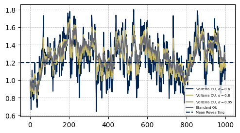
Figure D.1. Comparison of Volterra Ornstein-Uhlenbeck processes with parameter set $(x_{0},\alpha,b,\beta,\sigma)=(1,\alpha,1.2,-1,0.3)$ and $\alpha\in\{0.6,0.8,0.95,1\}$, for a fixed sample of pseudo random numbers. Here, $T=10$ and $\Delta t_{k+1}=0.01$.

VOU process with $\alpha=0.95$
Estimator	Mean	Median	Std
$\widehat{b}$	1.1983	1.1985	0.0645
$\widehat{\beta}$	-0.9988	-1.0000	0.0527
$\widehat{b}^{\text{mom}}$	0.9470	0.9470	0.0580
$\widehat{\beta}^{\text{mom}}$	-0.7890	-0.7883	0.0476
$\widehat{b}^{\beta}$	1.1997	1.1995	0.0136
$\widehat{\beta}^{b}$	-1.0003	-1.0003	0.0111

Table 1. VOU process with $T=500$, $\Delta t_{k+1}=0.5$, $\text{Factor}=1$.

VOU process with $\alpha=0.95$
Estimator	Mean	Median	Std
$\widehat{b}$	1.2059	1.2026	0.1033
$\widehat{\beta}$	-1.0046	-1.0007	0.0845
$\widehat{b}^{\text{mom}}$	1.2003	1.1951	0.1042
$\widehat{\beta}^{\text{mom}}$	-1.0005	-0.9969	0.0853
$\widehat{b}^{\beta}$	1.2004	1.2009	0.0172
$\widehat{\beta}^{b}$	-0.9998	-0.9995	0.0141

Table 2. VOU process with $T=500$, $\Delta t_{k+1}=0.05$, $\text{Factor}=1$.

VOU process with $\alpha=0.8$
Estimator	Mean	Median	Std
$\widehat{b}$	1,2046	1,1677	0,4084
$\widehat{\beta}$	-1,0055	-0,9844	0,3391
$\widehat{b}^{\text{mom}}$	1,9801	1,8663	0,786
$\widehat{\beta}^{\text{mom}}$	-1,6808	-1,5853	0,6533
$\widehat{b}^{\beta}$	1,1972	1,1965	0,0754
$\widehat{\beta}^{b}$	-1,0035	-1,003	0,0645

Table 3. VOU process with $T=15$, $\Delta t_{k+1}=0.05$, $\text{Factor}=2$.

VOU process with $\alpha=0.8$
Estimator	Mean	Median	Std
$\widehat{b}$	1,2047	1,1513	0,4019
$\widehat{\beta}$	-1,0045	-0,9732	0,3307
$\widehat{b}^{\text{mom}}$	1,6254	1,5357	0,5408
$\widehat{\beta}^{\text{mom}}$	-1,3818	-1,3173	0,4508
$\widehat{b}^{\beta}$	1,1985	1,1994	0,0766
$\widehat{\beta}^{b}$	-1,0026	-0,9983	0,0643

Table 4. VOU process with $T=15$, $\Delta t_{k+1}=0.01$, $\text{Factor}=2$.

VOU process with $\alpha=0.6$
Estimator	Mean	Median	Std
$\widehat{b}$	1.2914	1.1405	1.161
$\widehat{\beta}$	-1.0995	-1.0046	1.0553
$\widehat{b}^{\text{mom}}$	-	-	-
$\widehat{\beta}^{\text{mom}}$	-	-	-
$\widehat{b}^{\beta}$	1.185	1.1648	0.2842
$\widehat{\beta}^{b}$	-1.0362	-1.0199	0.2675

Table 5. VOU process with $T=1$, $\Delta t_{k+1}=0.01$, $\text{Factor}=4$.

VOU process with $\alpha=0.6$
Estimator	Mean	Median	Std
$\widehat{b}$	1.1456	0.9809	1.226
$\widehat{\beta}$	-0.949	-0.7999	1.0896
$\widehat{b}^{\text{mom}}$	-	-	-
$\widehat{\beta}^{\text{mom}}$	-	-	-
$\widehat{b}^{\beta}$	1.192	1.1868	0.2964
$\widehat{\beta}^{b}$	-1.0234	-0.9984	0.2728

Table 6. VOU process with $T=1$, $\Delta t_{k+1}=0.005$, $\text{Factor}=4$.

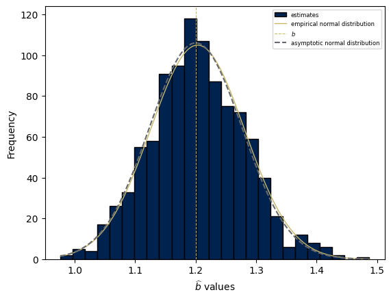
Figure D.2. VOU process with $\alpha=0.95$, $T=500$, $\Delta t_{k+1}=0.05$, $\text{Factor}=1$.

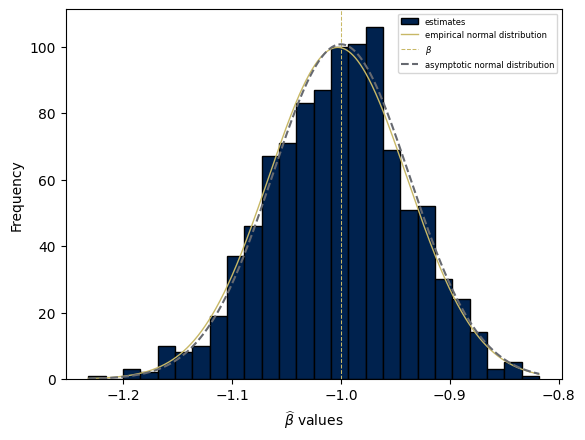
Figure D.3. VOU process with $\alpha=0.95$, $T=500$, $\Delta t_{k+1}=0.05$, $\text{Factor}=1$.

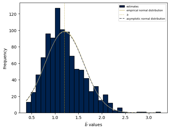
Figure D.4. VOU process with $\alpha=0.8$, $T=15$, $\Delta t_{k+1}=0.01$, $\text{Factor}=2$.

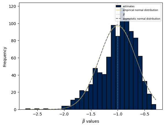
Figure D.5. VOU process with $\alpha=0.8$, $T=15$, $\Delta t_{k+1}=0.01$, $\text{Factor}=2$.

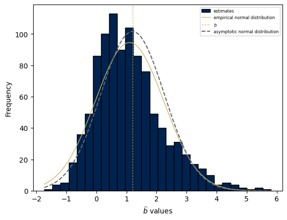
Figure D.6. VOU process with $\alpha=0.6$, $T=1$, $\Delta t_{k+1}=0.001$, $\text{Factor}=4$.

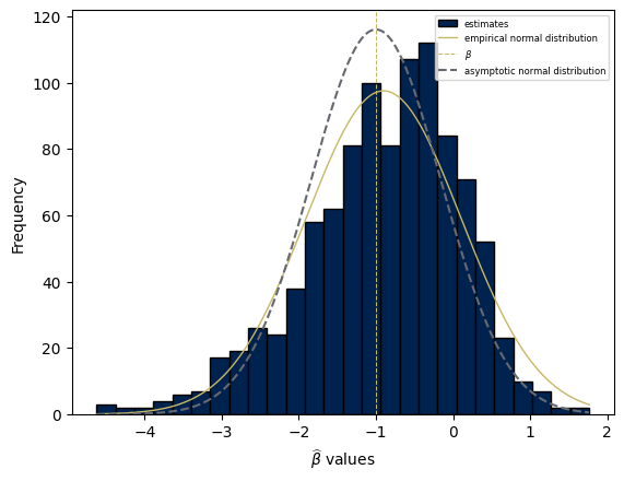
Figure D.7. VOU process with $\alpha=0.6$, $T=1$, $\Delta t_{k+1}=0.001$, $\text{Factor}=4$.

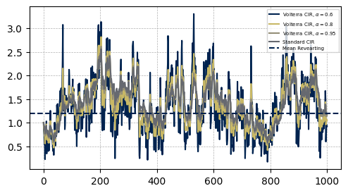
Figure D.8. Comparison of Volterra Cox-Ingersoll-Ross processes with parameter set $(x_{0},\alpha,b,\beta,\sigma)=(1,\alpha,1.2,-1,0.8)$ and $\alpha\in\{0.6,0.8,0.95,1\}$, for a fixed sample of pseudo random numbers. Here, $T=10$ and $\Delta t_{k+1}=0.01$.

VCIR process with $\alpha=0.95$ and $\sigma=0.6$
Estimator	Mean	Median	Std
$\widehat{b}$	1.1813	1.1795	0.0508
$\widehat{\beta}$	-0.9851	-0.9851	0.0468
$\widehat{b}^{\text{mom}}$	0.9331	0.932	0.0599
$\widehat{\beta}^{\text{mom}}$	-0.7779	-0.7755	0.051
$\widehat{b}^{\beta}$	1.1954	1.1944	0.021
$\widehat{\beta}^{b}$	-1.0011	-1.0011	0.0196

Table 7. VCIR process with $T=500$, $\Delta t_{k+1}=0.5$, $\text{Factor}=1$.

VCIR process with $\alpha=0.95$ and $\sigma=0.6$
Estimator	Mean	Median	Std
$\widehat{b}$	1.2008	1.1988	0.0669
$\widehat{\beta}$	-0.9988	-0.9968	0.0614
$\widehat{b}^{\text{mom}}$	1.1892	1.1906	0.0767
$\widehat{\beta}^{\text{mom}}$	-0.9902	-0.9908	0.0685
$\widehat{b}^{\beta}$	1.2014	1.2	0.0278
$\widehat{\beta}^{b}$	-0.9989	-0.9995	0.0255

Table 8. VCIR process with $T=500$, $\Delta t_{k+1}=0.05$, $\text{Factor}=1$.

VCIR process with $\alpha=0.8$ and $\sigma=0.8$
Estimator	Mean	Median	Std
$\widehat{b}$	1.1501	1.1064	0.3915
$\widehat{\beta}$	-0.9568	-0.9262	0.3726
$\widehat{b}^{\text{mom}}$	1.7488	1.6738	0.6174
$\widehat{\beta}^{\text{mom}}$	-1.5227	-1.4653	0.5871
$\widehat{b}^{\beta}$	1.166	1.1573	0.2445
$\widehat{\beta}^{b}$	-1.0328	-1.0128	0.1992

Table 9. VCIR process with $T=15$, $\Delta t_{k+1}=0.05$, $\text{Factor}=2$.

VCIR process with $\alpha=0.8$ and $\sigma=0.8$
Estimator	Mean	Median	Std
$\widehat{b}$	1.1674	1.0986	0.3836
$\widehat{\beta}$	-0.9711	-0.9343	0.3633
$\widehat{b}^{\text{mom}}$	1.6501	1.5724	0.5458
$\widehat{\beta}^{\text{mom}}$	-1.4361	-1.382	0.5043
$\widehat{b}^{\beta}$	1.1733	1.1536	0.2074
$\widehat{\beta}^{b}$	-1.0326	-1.0117	0.1909

Table 10. VCIR process with $T=15$, $\Delta t_{k+1}=0.01$, $\text{Factor}=2$.

VCIR process with $\alpha=0.6$ and $\sigma=0.8$
Estimator	Mean	Median	Std
$\widehat{b}$	1.1622	0.9118	1.4376
$\widehat{\beta}$	-0.0597	-0.3117	2.4683
$\widehat{b}^{\text{mom}}$	–	5–	–
$\widehat{\beta}^{\text{mom}}$	–	–	–
$\widehat{b}^{\beta}$	1.0778	0.9319	0.9515
$\widehat{\beta}^{b}$	-1.2725	-1.1391	0.8253

Table 11. VCIR process with $T=1$, $\Delta t_{k+1}=0.01$, $\text{Factor}=4$.

VCIR process with $\alpha=0.6$ and $\sigma=0.8$
Estimator	Mean	Median	Std
$\widehat{b}$	0.9277	0.6861	1.2994
$\widehat{\beta}$	-0.1153	-0.2514	2.321
$\widehat{b}^{\text{mom}}$	–	–	–
$\widehat{\beta}^{\text{mom}}$	–	–	–
$\widehat{b}^{\beta}$	1.0296	0.9262	1.0131
$\widehat{\beta}^{b}$	-1.2482	-1.0948	0.8637

Table 12. VCIR process with $T=1$, $\Delta t_{k+1}=0.005$, $\text{Factor}=4$.

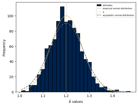
Figure D.9. VCIR process with $\alpha=0.95$, $\sigma=0.6$, $T=500$, $\Delta t_{k+1}=0.05$, $\text{Factor}=1$.

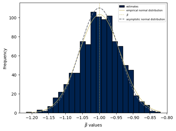
Figure D.10. VCIR process with $\alpha=0.95$, $\sigma=0.6$, $T=500$, $\Delta t_{k+1}=0.05$, $\text{Factor}=1$.

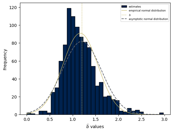
Figure D.11. VCIR process with $\alpha=0.8$, $\sigma=0.8$, $T=15$, $\Delta t_{k+1}=0.01$, $\text{Factor}=2$.

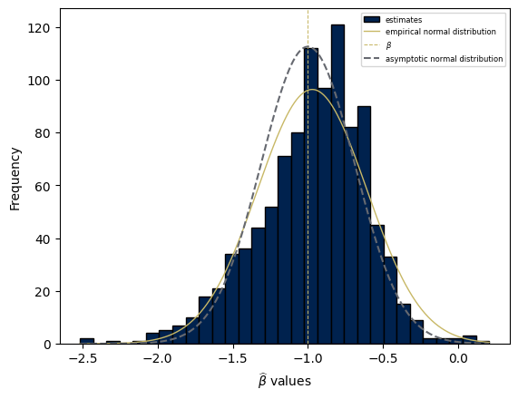
Figure D.12. VCIR process with $\alpha=0.8$, $\sigma=0.8$, $T=15$, $\Delta t_{k+1}=0.01$, $\text{Factor}=2$.

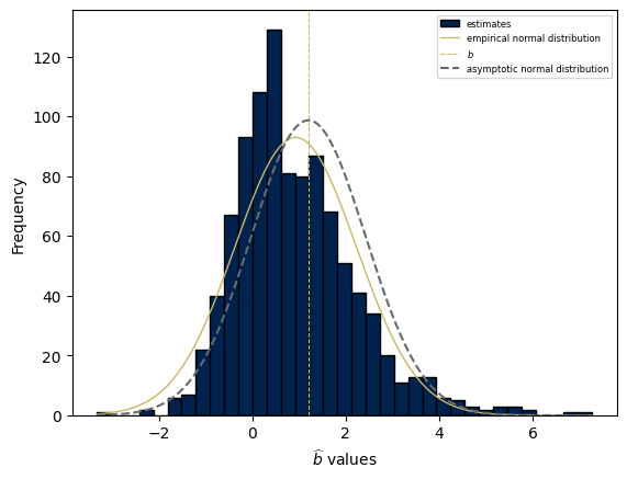
Figure D.13. VCIR process with $\alpha=0.6$, $\sigma=0.8$, $T=1$, $\Delta t_{k+1}=0.001$, $\text{Factor}=4$.

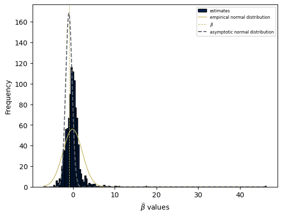
Figure D.14. VCIR process with $\alpha=0.6$, $\sigma=0.8$, $T=1$, $\Delta t_{k+1}=0.001$, $\text{Factor}=4$.

Acknowledgement

M. F. would like to thank the LMRS for the wonderful hospitality and Financial support in 2023 during which a large part of the research was carried out. Moreover, M.F. gratefully acknowledges the Financial support received from Campus France awarded by Ambassade de France en Irlande to carry out the project “Parameter estimation in affine rough models”.

References

• [1] Eduardo Abi Jaber and Omar El Euch, Multifactor approximation of rough volatility models, SIAM J. Financial Math. 10 (2019), no. 2, 309–349. MR 3934104
• [2] Eduardo Abi Jaber, Martin Larsson, and Sergio Pulido, Affine Volterra processes, Ann. Appl. Probab. 29 (2019), no. 5, 3155–3200. MR 4019885
• [3] Aurélien Alfonsi, Nonnegativity preserving convolution kernels. application to stochastic volterra equations in closed convex domains and their approximation, 2023.
• [4] Aurélien Alfonsi and Ahmed Kebaier, Approximation of stochastic volterra equations with kernels of completely monotone type, Mathematics of Computation 93 (2024), no. 346, 643–677.
• [5] Mátyás Barczy, Leif Döring, Zenghu Li, and Gyula Pap, On parameter estimation for critical affine processes, Electron. J. Stat. 7 (2013), 647–696. MR 3035268
• [6] by same author, Parameter estimation for a subcritical affine two factor model, J. Statist. Plann. Inference 151/152 (2014), 37–59. MR 3216637
• [7] Christian Bayer and Simon Breneis, Markovian approximations of stochastic Volterra equations with the fractional kernel, Quant. Finance 23 (2023), no. 1, 53–70. MR 4521278
• [8] Christian Bayer, Peter Friz, and Jim Gatheral, Pricing under rough volatility, Quant. Finance 16 (2016), no. 6, 887–904. MR 3494612
• [9] Mohamed Ben Alaya, Houssem Dahbi, and Hamdi Fathallah, Asymptotic properties of $ad(1,n)$ model and its maximum likelihood estimator, arXiv:2303.08467 (2023), 1–22.
• [10] Mohamed Ben Alaya and Ahmed Kebaier, Asymptotic behavior of the maximum likelihood estimator for ergodic and nonergodic square-root diffusions, Stochastic Analysis and Applications 31 (2013), no. 4, 552–573.
• [11] Viktor Bengs and Hajo Holzmann, Uniform approximation in classical weak convergence theory, arXiv:1903.09864 (2019).
• [12] Abdel Berkaoui, Mireille Bossy, and Awa Diop, Euler scheme for sdes with non-lipschitz diffusion coefficient: strong convergence, ESAIM: Probability and Statistics 12 (2008), no. 1, 1–11.
• [13] Luigi Amedeo Bianchi, Stefano Bonaccorsi, and Martin Friesen, Limits of stochastic volterra equations driven by gaussian noise, arXiv:2311.07358 (2023).
• [14] Richard C. Bradley, Basic properties of strong mixing conditions. A survey and some open questions, Probab. Surv. 2 (2005), 107–144, Update of, and a supplement to, the 1986 original. MR 2178042
• [15] Etienne Chevalier, Sergio Pulido, and Elizabeth Zúñiga, American options in the Volterra Heston model, SIAM J. Financial Math. 13 (2022), no. 2, 426–458. MR 4412586
• [16] Giulia Di Nunno, Kȩstutis Kubilius, Yuliya Mishura, and Anton Yurchenko-Tytarenko, From constant to rough: A survey of continuous volatility modeling, Mathematics 11 (2023), no. 19.
• [17] D. Duffie, D. Filipović, and W. Schachermayer, Affine processes and applications in finance, Ann. Appl. Probab. 13 (2003), no. 3, 984–1053. MR 1994043
• [18] Omar El Euch, Masaaki Fukasawa, and Mathieu Rosenbaum, The microstructural foundations of leverage effect and rough volatility, Finance Stoch. 22 (2018), no. 2, 241–280. MR 3778355
• [19] Omar El Euch and Mathieu Rosenbaum, The characteristic function of rough Heston models, Math. Finance 29 (2019), no. 1, 3–38. MR 3905737
• [20] Martin Friesen, Regular occupation measures of volterra processes, arXiv: (2024).
• [21] Martin Friesen and Peng Jin, Volterra square-root process: Stationarity and regularity of the law, The Annals of Applied Probability 34 (2024), no. 1A, 318 – 356.
• [22] Martin Friesen, Peng Jin, Jonas Kremer, and Barbara Rüdiger, Exponential ergodicity for stochastic equations of nonnegative processes with jumps, ALEA Lat. Am. J. Probab. Math. Stat. 20 (2023), no. 1, 593–627. MR 4567723
• [23] by same author, Regularity of transition densities and ergodicity for affine jump-diffusions, Math. Nachr. 296 (2023), no. 3, 1117–1134. MR 4585666
• [24] Martin Friesen, Peng Jin, and Barbara Rüdiger, Stochastic equation and exponential ergodicity in Wasserstein distances for affine processes, Ann. Appl. Probab. 30 (2020), no. 5, 2165–2195. MR 4149525
• [25] Masaaki Fukasawa, Volatility has to be rough, Quant. Finance 21 (2021), no. 1, 1–8. MR 4188876
• [26] Jim Gatheral, Thibault Jaisson, and Mathieu Rosenbaum, Volatility is rough, Quant. Finance 18 (2018), no. 6, 933–949. MR 3805308
• [27] Stefan Gerhold, Christoph Gerstenecker, and Arpad Pinter, Moment explosions in the rough Heston model, Decis. Econ. Finance 42 (2019), no. 2, 575–608. MR 4031338
• [28] G. Gripenberg, S.-O. Londen, and O. Staffans, Volterra integral and functional equations, Encyclopedia of Mathematics and its Applications, vol. 34, Cambridge University Press, Cambridge, 1990. MR 1050319
• [29] El Mehdi Haress and Yaozhong Hu, Estimation of all parameters in the fractional Ornstein-Uhlenbeck model under discrete observations, Stat. Inference Stoch. Process. 24 (2021), no. 2, 327–351. MR 4265053
• [30] Blanka Horvath, Antoine Jacquier, and Peter Tankov, Volatility options in rough volatility models, SIAM J. Financial Math. 11 (2020), no. 2, 437–469. MR 4091168
• [31] Yaozhong Hu and David Nualart, Parameter estimation for fractional Ornstein-Uhlenbeck processes, Statist. Probab. Lett. 80 (2010), no. 11-12, 1030–1038. MR 2638974
• [32] Yaozhong Hu, David Nualart, and Hongjuan Zhou, Drift parameter estimation for nonlinear stochastic differential equations driven by fractional Brownian motion, Stochastics 91 (2019), no. 8, 1067–1091. MR 4023508
• [33] by same author, Parameter estimation for fractional Ornstein-Uhlenbeck processes of general Hurst parameter, Stat. Inference Stoch. Process. 22 (2019), no. 1, 111–142. MR 3918739
• [34] Yury A. Kutoyants, Statistical inference for ergodic diffusion processes, Springer Series in Statistics, Springer-Verlag London, Ltd., London, 2004. MR 2144185
• [35] Zenghu Li and Chunhua Ma, Asymptotic properties of estimators in a stable Cox-Ingersoll-Ross model, Stochastic Process. Appl. 125 (2015), no. 8, 3196–3233. MR 3343292
• [36] Robert S. Liptser and Albert N. Shiryaev, Statistics of random processes. I., expanded ed., Applications of Mathematics (New York), vol. 5, Springer-Verlag, Berlin, 2001, General theory, Translated from the 1974 Russian original by A. B. Aries, Stochastic Modelling and Applied Probability. MR 1800857
• [37] Eberhard Mayerhofer, Robert Stelzer, and Johanna Vestweber, Geometric ergodicity of affine processes on cones, Stochastic Process. Appl. 130 (2020), no. 7, 4141–4173. MR 4102262
• [38] Yuliya Mishura and Anton Yurchenko-Tytarenko, Parameter estimation in rough bessel model, Fractal and Fractional 7 (2023), no. 7.
• [39] Fabien Panloup, Samy Tindel, and Maylis Varvenne, A general drift estimation procedure for stochastic differential equations with additive fractional noise, Electron. J. Stat. 14 (2020), no. 1, 1075–1136. MR 4068875
• [40] Viet Son Pham and Carsten Chong, Volterra-type Ornstein-Uhlenbeck processes in space and time, Stochastic Process. Appl. 128 (2018), no. 9, 3082–3117. MR 3834854
• [41] Gennady Samorodnitsky, Stochastic processes and long range dependence, Springer Series in Operations Research and Financial Engineering, Springer, Cham, 2016. MR 3561100
• [42] Nikola Sandrić, A note on the Birkhoff ergodic theorem, Results Math. 72 (2017), no. 1-2, 715–730. MR 3684455
• [43] Elizabeth Zuniga, Volterra processes and applications in finance, V. General Mathematics [math.GM]. Université Paris-Saclay, 2021. (2021), 37–59.