B-ary Tree Push-Pull Method is Provably Efficient for Decentralized Learning on Heterogeneous Data

Abstract

This paper considers the distributed learning problem where a group of agents cooperatively minimizes the summation of their local cost functions based on peer-to-peer communication. Particularly, we propose a highly efficient algorithm, termed “B-ary Tree Push-Pull” (BTPP), that employs two B-ary spanning trees for distributing the information related to the parameters and stochastic gradients across the network. The simple method is efficient in communication since each agent interacts with at most $(B+1)$ neighbors per iteration. More importantly, BTPP achieves linear speedup for smooth nonconvex objective functions with only $\tilde{O}(n)$ transient iterations, significantly outperforming the state-of-the-art results to the best of our knowledge.

1 Introduction

In this paper, we consider a group of agents, labeled as ${\mathcal{N}}:=\{1,2,\ldots,n\}$, in which each agent $i$ holds its own local cost function $f_{i}:\mathbb{R}^{p}\rightarrow\mathbb{R}$ and communicates only within its direct neighborhood. We investigate how the agents collaborate to locate $x\in\mathbb{R}^{p}$ that minimizes the average of all the cost functions:

$$\min_{x\in\mathbb{R}^{p}}f(x)\left(=\frac{1}{n}\sum_{i=1}^{n}f_{i}(x)\right),$$ (1)

where $f_{i}(x):=\mathbb{E}_{\xi_{i}\sim{\mathcal{D}}_{i}}\left[F_{i}(x;\xi_{i})\right]$. Here $\xi_{i}$ denotes the local data of agent $i$ that follows the local distribution ${\mathcal{D}}_{i}$. Data heterogeneity exists if $\left\{{\mathcal{D}}_{i}\right\}_{i=1}^{n}$ are not identical.

To solve problem (1), we assume each agent $i$ queries a stochastic oracle (${\mathcal{S}}{\mathcal{O}}$) to obtain noisy gradient samples. Stochastic gradients appear in many areas including online distributed learning [23, 3], reinforcement learning [17, 15], generative modeling [5, 6], and parameter estimation [2, 27]. 1.1 ensures that the gradient estimator $g_{i}(x;\xi_{i})$ remains unbiased with a bounded variance for any given ${\mathbf{x}}$, while independent samples $\xi_{i}$ are gathered continuously over time. In addition, the assumption is critical in simulation-based optimization as gradient estimation often encounters noise from multiple sources, such as modeling and discretization errors, or limitations due to finite sample sizes in Monte-Carlo methods [7].

Modern optimization and machine learning typically involve tremendous data samples and model parameters. The scale of these problems calls for efficient distributed algorithms across multiple computing nodes. Recently, distributed algorithms dealing with problem (1) have been studied extensively in the literature; see, e.g., [19, 14, 4, 34]. Traditional distributed learning approaches typically follow a centralized master-worker setup, where each worker node communicates with a (virtual) central server [12]. However, such a communication pattern incurs significant communication overheads and long latency, especially when the training requires a large number of computing nodes.

Decentralized learning is an emerging paradigm to save communication costs, where the computing nodes are connected through a certain network topology (e.g., ring, grid, hypercube). Decentralized algorithms do not rely on central servers: the agents maintain the similarity among their copies of model parameters through peer-to-peer messages passing by communicating locally with immediate neighbors in the network. Such a setup allows each node to communicate with only a few peers and hence incurs much lower communication overhead [1]. Moreover, it offers strong promise for new applications, allowing agents to collaboratively train a model while respecting the data locality and privacy of each contributor.

Specifically, in decentralized stochastic gradient methods, the agents share their local stochastic gradient updates through gossip communication [32]. At every iteration, the local updates are sent to the neighbors of each agent who iteratively propagate the information through the network. Typically, the agents employ iterative gossip averaging of their neighbors’ models with their own, where the averaging weights are chosen to ensure asymptotic uniform distribution of each update across the network. However, local averaging is less effective in “mixing” information which makes decentralized algorithms converge slower than their centralized counterparts. Generally speaking, the network topology determines both the number of per-iteration communications and the convergence rates of decentralized algorithms, leading to a trade-off. For example, a densely-connected graph enables decentralized methods to converge faster but results in less efficient communication since each node needs to communicate with more neighbors. By contrast, a sparsely-connected topology results in a slower convergence rate but also reduces the per-iteration communication cost [19, 21, 35]. In particular, for smooth and non-convex objective functions, it has been shown that decentralized stochastic gradient methods (with arbitrary topology) can achieve the same convergence rate as the centralized SGD method, but only after an initial period of iterations has passed [14, 34, 20]. The number of transient iterations (transient time) heavily depends on the network topology, and thus a practical decentralized stochastic gradient algorithm should aim to minimize the transient time while keeping the number of per-iteration communications small (e.g., over a a sparsely-connected topology). Such an observation has motivated several recent works, which consider network topologies with $\Theta(1)$ per-iteration communications (or degree) for each node; see, e.g., [34, 26].

This work considers an alternative mechanism to gossip averaging, called “B-ary Tree Push-Pull” (BTPP), inherited from the Push-Pull method in [22, 33]. Rather than relaying the messages over one graph at every iteration, BTPP uses two B-ary trees (${\mathcal{G}}_{{\mathcal{R}}}$ and ${\mathcal{G}}_{{\mathcal{C}}}$) to spread the information about the parameters and the stochastic gradients, respectively. Each agent assigned in the B-ary tree acts as a worker on an assembly line. The model parameters are transmitted through the graph ${\mathcal{G}}_{{\mathcal{R}}}$ from the parent nodes to the child nodes. Meanwhile, the stochastic gradients are computed under the current model parameters and accumulated through the inverse graph of ${\mathcal{G}}_{{\mathcal{R}}}$ denoted as ${\mathcal{G}}_{{\mathcal{C}}}$. BTPP can be viewed as a semi-(de)centralized approach given the critical role of node $1$. Notably, the corresponding mixing matrices of ${\mathcal{G}}_{{\mathcal{R}}}$ and ${\mathcal{G}}_{{\mathcal{C}}}$ only consist of $0$’s and $1$’s, which together with the B-ary Tree topology design, results in high algorithmic efficiency. We show BTPP achieves an $\tilde{{\mathcal{O}}}(n)$ transient time under smooth nonconvex objective functions with $\Theta(1)$ per-iteration communications for each agent. By comparison, the state-of-the-art transient time is ${\mathcal{O}}(n^{3})$ (see Table 1).

1.1 Related Works

Decentralized Learning

Decentralized Stochastic Gradient Descent (DSGD) type algorithms are increasingly popular for accelerating the training of large-scale machine learning models [14, 34, 10] . These algorithms have been adapted under a range of practical settings, including those discussed in [1, 16]. However, DSGD suffers from data heterogeneity [9], which triggers more advanced techniques such as EXTRA [25], Exact-Diffusion/$\text{D}^{2}$ [13], and gradient tracking [19]. The Push-Pull method [22, 33] which enjoys broad topological requirements was introduced for deterministic decentralized optimization under strongly convex objectives. This work particularly takes advantage of the flexibility in the network design of Push-Pull, utilizing the B-ary tree family, while considering stochastic gradients for minimizing smooth nonconvex objectives.

Topology Design

Decentralized stochastic gradient algorithms often rely on gossip averaging over various topologies such as rings, grids, and tori [18]. The hypercube graph [30] strikes a balance between the communication efficiency and the consensus rate, but the network size is constrained to be the power of two. The work in [34] re-examined the static exponential graph with $\Theta(\ln(n))$ degree and introduced a one-peer exponential graph with $\Theta(1)$ degree while preserving the consensus properties under the specific requirement of $n$. The paper [28] proposed a base-($k+1$) graph as an enhancement that achieves similar convergence rate as in [34] under arbitrary network size by sequentially employing multiple graph topologies (splitting an all-connected graph into $\Theta(\ln(n))$ different subgraphs). DSGD-CECA [4] requires roughly $\lceil\log_{2}(n)\rceil$ rounds of message passing for global averaging with $\Theta(n)$ network topologies. OD(OU)-EquiDyn [26] introduces algorithms that employ various topologies to achieve network-size independent consensus rates. RelaySGD [31] offers a relay-based algorithm that ensures $\Theta(1)$ per-iteration communication across different topologies.

The above-mentioned methods all enjoy comparable convergence rates with centralized SGD (and thus achieves linear speedup) when the number of iterations $T$ is large enough. The transient times are generally in the order of $\tilde{{\mathcal{O}}}(n^{3})$ (see Table 1).

Note that the above works and this paper generally consider training machine learning modes within high-performance data-center clusters, in which the network topology can be fully controlled: any two nodes can directly communicate over the network when necessary. By comparison, in some other scenarios, the underlying network topology is fixed, and the communication between two nodes is constrained (e.g., in wireless sensor networks, internet of vehicles, etc).

Algorithm	Per-iter Comm.	Size $n$	Based Graph	Trans. Iter.
$D^{2}$ (Ring) [29]	$\Theta(1)$	arbitrary	1	${\mathcal{O}}(n^{11})$
DSGD (Ring) [18]	$\Theta(1)$	arbitrary	1	${\mathcal{O}}(n^{7})$
Hypercube [30]	$\Theta(\ln(n))$	power of 2	1	$\tilde{{\mathcal{O}}}(n^{3})$
Static Exp. [34]	$\Theta(\ln(n))$	arbitrary	1	$\tilde{{\mathcal{O}}}(n^{3})$
O.-P. Exp. [34]	1	power of 2	$\Theta(\ln(n))$	$\tilde{{\mathcal{O}}}(n^{3})$
RelaySGD [31]	$\Theta(1)$	arbitrary	1	${\mathcal{O}}(n^{3})$
OD(OU)-EquiDyn [26]	1	arbitrary	$\Theta(n)$	${\mathcal{O}}(n^{3})$
DSGD-CECA [4]	$\Theta(1)$	arbitrary	$\Theta(n)$	$\tilde{{\mathcal{O}}}(n^{3})$
Base-($k+1$) [28]	$\Theta(1)$	arbitrary	$\Theta(\ln(n))$	$\tilde{{\mathcal{O}}}(n^{3})$
$\bm{B}$-ary Tree (Ours)	$\bm{\Theta(1)}$	arbitrary	2	$\bm{\tilde{{\mathcal{O}}}(n)}$

Table 1: Comparison of different algorithms for distributed stochastic optimization under smooth nonconvex objectives. “Per-iter Comm.” denotes the number of per-iteration communications or neighbors (degree) for each agent. “Based Graph” represents the number of required graph topologies during the entire training procedure. “Trans. Iter.” represents the number of transient iterations. The notation $\tilde{{\mathcal{O}}}(\cdot)$ hides all the polylogarithmic factors.

1.2 Main Contribution

This paper introduces a novel distributed stochastic gradient algorithm, termed “B-ary Tree Push-Pull” (BTPP), which is provably efficient for solving the distributed learning problem (1) under arbitrary network size. The main contribution is summarized as follows:

• BTPP incurs a $\Theta(1)$ communication overhead per-iteration for each agent. Specifically, any agent in the network communicates with at most $(B+1)$ neighbors, where $B$ can be freely chosen to fit different settings. Generally speaking, larger $B$ increases the per-iteration communication cost but reduces the transient time at the same time.

• We show BTPP enjoys an $\tilde{{\mathcal{O}}}(n)$ transient time or iteration complexity under smooth nonconvex objectives. Such a result outperforms the baselines: see Table 1. The improvement is significant since the transient time greatly impacts the algorithmic performance, especially under large $n$.

• The convergence analysis for BTPP is non-trivial, partly due to the fact that the algorithm admits two different network topologies for communicating the model parameters and the (stochastic) gradient trackers respectively. Instead of constructing the induced matrix norms $\|\cdot\|_{{\mathcal{R}}}$ and $\|\cdot\|_{{\mathcal{C}}}$ as in [22], the analysis is performed under $\left\|\cdot\right\|_{2}$ and $\left\|\cdot\right\|_{F}$ only by carefully treating the matrix products and related terms.

1.3 Notation and Preliminaries

Throughout the paper, vectors default to columns if not otherwise specified. Let each agent $i$ hold a local copy $x_{i}\in\mathbb{R}^{p}$ of the decision variable and an auxiliary variable $y_{i}\in\mathbb{R}^{p}$. Their values at iteration $k$ are denoted by $x_{i}^{(k)}$ and $y_{i}^{(k)}$, respectively. We let

$${\mathbf{X}}=\left[x_{1},x_{2},\cdots,x_{n}\right]^{\top}\in\mathbb{R}^{n\times p},\;{\mathbf{Y}}=\left[y_{1},y_{2},\cdots,y_{n}\right]^{{\mathrm{T}}}\in\mathbb{R}^{n\times p},$$

and $\mathbbm{1}$ denotes the column vector with all entries equal to 1. We also define the aggregated gradients at the local variables as

$$\nabla F({\mathbf{X}}):=\left[\nabla f_{1}(x_{1}),\nabla f_{2}(x_{2}),\cdots,\nabla f_{n}(x_{n})\right]^{{\mathrm{T}}}\in\mathbb{R}^{n\times p},$$

where $F({\mathbf{X}}):=\sum_{i=1}^{n}f_{i}(x_{i})$. In addition, denote

$${\bm{\xi}}:=\left[\xi_{1},\xi_{2},\cdots,\xi_{n}\right]^{{\mathrm{T}}},\;{\mathbf{G}}({\mathbf{X}},{\bm{\xi}}):=\left[g_{1}(x_{1},\xi_{1}),g_{2}(x_{2},\xi_{2}),\cdots,g_{n}(x_{n},\xi_{n})\right]^{{\mathrm{T}}}\in\mathbb{R}^{n\times p}.$$

For the conciseness of presentation, we also use ${\mathbf{G}}^{(t)}$ to represent ${\mathbf{G}}({\mathbf{X}}^{(t)},{\bm{\xi}}^{(t)})$. The term $\langle a,b\rangle$ stands for the inner product of two vectors $a,b\in\mathbb{R}^{p}$. For matrices, $\left\|\cdot\right\|_{2}$ and $\left\|\cdot\right\|_{F}$ represent the spectral norm and the Frobenius norm respectively, which degenerate to the Euclidean norm for vectors. For simplicity, any square matrix with power $0$ is the unit matrix ${\mathbf{I}}$ with the same dimension if not otherwise specified.

We assume each agent $i$ is able to obtain noisy gradient samples of the form $g_{i}(x,\xi_{i})$ that satisfies the following assumption.

Assumption 1.1.

For all $i\in{\mathcal{N}}$ and $x\in\mathbb{R}^{p}$, each random vector $\xi_{i}$ is independent and

$$\mathbb{E}_{\xi_{i}\sim{\mathcal{D}}_{i}}\left[g_{i}(x,\xi_{i})|x\right]=\nabla f_{i}(x)$$

$$\mathbb{E}_{\xi_{i}\sim{\mathcal{D}}_{i}}\left[\left\|g_{i}(x,\xi_{i})-\nabla f_{i}(x)\right\|^{2}|x\right]\leq\sigma^{2}$$

for some $\sigma^{2}>0$.

Regarding the individual objective functions $f_{i}$, we make the following standard assumption.

Assumption 1.2.

Each $f_{i}(x):\mathbb{R}^{p}\rightarrow\mathbb{R}$ is lower bounded with $L$-Lipschitz continuous gradients, i.e., for any $x,x^{\prime}\in\mathbb{R}^{p}$,

$$\left\|\nabla f_{i}(x)-\nabla f_{i}(x^{\prime})\right\|\leq L\left\|x-x^{\prime}\right\|.$$

Denote $f^{*}:=\min_{x\in\mathbb{R}^{p}}f(x)$.

A directed graph ${\mathcal{G}}({\mathcal{N}},{\mathcal{E}})$ consists of a set of $n$ nodes ${\mathcal{N}}$ and a set of directed edges ${\mathcal{E}}\subseteq{\mathcal{N}}\times{\mathcal{N}}$, where an edge $(j,i)\in{\mathcal{E}}$ indicates that node $j$ can directly send information to node $i$. To facilitate the local averaging procedure, each graph can be associated with a non-negative weight matrix ${\mathbf{W}}=\left[w_{ij}\right]\in\mathbb{R}^{n\times n}$, whose element $w_{ij}$ is non-zero only if $(j,i)\in{\mathcal{E}}$. Similarly, a non-negative weight matrix ${\mathbf{W}}$ corresponds to a directed graph denoted by ${\mathcal{G}}_{\mathbf{W}}$. For a given graph ${\mathcal{G}}_{\mathbf{W}}$, the in-neighborhood and out-neighborhood of node $i\in{\mathcal{N}}$ are given by ${\mathcal{N}}_{{\mathbf{W}},i}^{in}:=\{j\in{\mathcal{N}}:(j,i)\in{\mathcal{E}}\}$ and ${\mathcal{N}}_{{\mathbf{W}},i}^{out}:=\{j\in{\mathcal{N}}:(i,j)\in{\mathcal{E}}\}$, respectively. The degree of node $i$ is the number of its in-neighbors or out-neighbors. For example, in a one-peer graph, the degree of each node is at most $1$.

1.4 Organization of the Paper

The rest of this paper is organized as follows. In section 2, we introduce the B-ary Tree Push-Pull algorithm and present its main convergence results. The sketch of analysis is presented in section 3, and numerical experiments are provided in section 4. We conclude the paper in section 5.

2 B-ary Tree Push-Pull Method

2.1 Communication Graphs

The proposed B-ary Tree Push-Pull method makes use of two spanning trees as communication graphs: ${\mathcal{G}}_{{\mathcal{R}}}$ and ${\mathcal{G}}_{{\mathcal{C}}}$, which correspond to two mixing matrices ${\mathcal{R}}$ and ${\mathcal{C}}$, respectively. Specifically, we consider B-ary tree graphs with arbitrary number of nodes $n$ and depth $d$. The root node is labeled as $1$ for convenience, and we index the nodes layer-by-layer. The additional nodes are placed at the last layer if the tree is not full. Figure 2 and Figure 2 illustrate the assignment of nodes when $B=2$. In the Pull Tree ${\mathcal{G}}_{{\mathcal{R}}}$ (the left ones), each node has $1$ parent node and $B$ child nodes (except the ones in the last layer). The root node $1$ has no parent node. In the Push Tree ${\mathcal{G}}_{{\mathcal{C}}}$ (the right ones), each node has $1$ child node and $B$ parent nodes (except the ones in the last layer). It can be seen that the tree ${\mathcal{G}}_{{\mathcal{C}}}$ is identical to ${\mathcal{G}}_{{\mathcal{R}}}$ with all the edges reversing directions. Note that only node 1 has a self-loop.

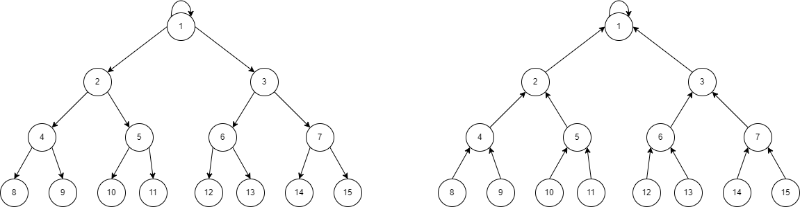
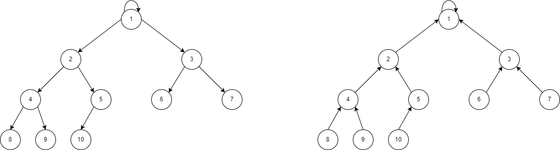
Figure 1: Two spanning trees with $16$ nodes when $B=2$. On the left is ${\mathcal{G}}_{{\mathcal{R}}}$, and the right one is ${\mathcal{G}}_{{\mathcal{C}}}$.

Figure 2: Two spanning trees with $10$ nodes when $B=2$. On the left is ${\mathcal{G}}_{{\mathcal{R}}}$, and the right one is ${\mathcal{G}}_{{\mathcal{C}}}$.

2.2 Algorithm

We consider the following distributed stochastic gradient method (Algorithm 1) for solving problem (1). At every iteration $t$, each agent $i$ pulls the state information from its in-neighborhood ${\mathcal{N}}_{{\mathcal{R}},i}^{in}$, pushes its (stochastic) gradient tracker $y_{i}$ to the out-neighborhood ${\mathcal{N}}_{{\mathcal{C}},i}^{out}$, and updates its local variables $x_{i}$ and $y_{i}$ based on the received information. The agents aim to find the $\epsilon$-stationary point jointly by performing local computation and exchanging information through two spanning trees.

Algorithm 1 B-ary Tree Push-Pull Method (BTPP)

1:Each agent $i$ initializes with any arbitrary but identical $x_{i}^{(0)}=x^{(0)}\in\mathbb{R}^{p}$, $y_{i}^{(0)}=g_{i}(x_{i}^{(0)},\xi_{i}^{(0)})\in\mathbb{R}^{p}$ after drawing a random sample $\xi_{i}^{(0)}$, stepsize $\gamma>0$ and number of iterations $T$.

2:for iteration $t=0,1,2,\ldots,T-1$ do

3:     for agent $i$ in parallel do

4:         Pull $x_{j}^{(t)}-\gamma y_{j}^{(t)}$ from each $j\in{\mathcal{N}}_{{\mathcal{R}},i}^{in}$

5:         Push $y_{i}^{(t)}$ to each $j\in{\mathcal{N}}_{{\mathcal{C}},i}^{out}$

6:         Independently draw a random sample $\xi_{i}^{(t+1)}$

7:         Update parameters through

$$x_{i}^{(t+1)} =\sum_{j\in{\mathcal{N}}_{{\mathcal{R}},i}^{in}}\left(x_{j}^{(t)}-\gamma y_{j}^{(t)}\right)$$

$$y_{i}^{(t+1)} =\sum_{j\in{\mathcal{N}}_{{\mathcal{C}},i}^{in}}y_{j}^{(t)}+g_{i}(x^{(t+1)}_{i};\xi_{i}^{(t+1)})-g_{i}(x^{(t)}_{i};\xi_{i}^{(t)})$$

8:     end for

9:end for

10:Output $x_{1}^{(T)}$.

More specifically, in the pull tree ${\mathcal{G}}_{{\mathcal{R}}}$, each node $i$ pulls the updated model from its parent node along the tree. Note that ${\mathcal{N}}_{{\mathcal{R}},i}^{in}$ consists of only one node, the parent node. The Push Tree ${\mathcal{G}}_{{\mathcal{C}}}$ is the inverse of the Pull Tree, in which each node collects and aggregates the gradient trackers from its parent nodes. Due to the tree structure, only $y_{1}^{t}$ aggregates and tracks the stochastic gradients across the entire network, which will be made clear from the analysis. The implementation of the algorithm is rather simple. Taking node $2$ in Figure 2 as an example, we have $x_{2}^{(t+1)}=x_{1}^{(t)}-\gamma y_{1}^{(t)}$ and $y_{2}^{(t+1)}=y_{4}^{(t)}+y_{5}^{(t)}+g_{2}(x^{(t+1)}_{2};\xi_{2}^{(t+1)})-g_{2}(x^{(t)}_{2};\xi_{2}^{(t)})$.

We can write Algorithm 1 in the following compact form:

$${\mathbf{X}}^{(t+1)} ={\mathcal{R}}\left({\mathbf{X}}^{(t)}-\gamma{\mathbf{Y}}^{(t)}\right)$$ (2)

$${\mathbf{Y}}^{(t+1)} ={\mathcal{C}}{\mathbf{Y}}^{(t)}+{\mathbf{G}}({\mathbf{X}}^{(t+1)},{\bm{\xi}}^{(t+1)})-{\mathbf{G}}({\mathbf{X}}^{(t)},{\bm{\xi}}^{(t)})$$

where ${\mathbf{Y}}^{(0)}={\mathbf{G}}({\mathbf{X}}^{(0)},{\bm{\xi}}^{(0)})$, and ${\mathcal{R}},{\mathcal{C}}\in\mathbb{R}^{n\times n}$ are non-negative matrices whose elements are given by

$$\left[{\mathcal{R}}\right]_{i,j}=\left\{\begin{aligned} 1&\quad\text{if }i\in\left\{Bj+1-B+[B]\right\}\cap[n]\\ 0&\quad\text{otherwise}\end{aligned}\right.$$

and ${\mathcal{C}}={\mathcal{R}}^{{\mathrm{T}}}$ which corresponds to ${\mathcal{G}}_{{\mathcal{C}}}$, the inverse tree of ${\mathcal{G}}_{{\mathcal{R}}}$. It can be seen that ${\mathcal{R}}$ is a row-stochastic matrix that only consists of $0$’s and $1$’s, and ${\mathcal{C}}$ is column stochastic. For example, the mixing matrices corresponding to the graphs in Figure 2 are given by

$${\mathcal{R}}=\left(\begin{matrix}1&&&&&&&&&\\ 1&&&&&&&&&\\ 1&&&&&&&&&\\ &1&&&&&&&&\\ &1&&&&&&&&\\ &&1&&&&&&&\\ &&1&&&&&&&\\ &&&1&&&&&&\\ &&&1&&&&&&\\ &&&&1&&&&&\\ \end{matrix}\right),\quad{\mathcal{C}}=\left(\begin{matrix}1&1&1&&&&&&&\\ &&&1&1&&&&&\\ &&&&&1&1&&&\\ &&&&&&&1&1&\\ &&&&&&&&&1\\ &&&&&&&&&\\ &&&&&&&&&\\ &&&&&&&&&\\ &&&&&&&&&\\ &&&&&&&&&\\ \end{matrix}\right),$$

where the unspecified elements are zeros.

2.3 Main Result

The main convergence properties of BTPP are summarized in the following theorem.

Theorem 2.1.

For the BTPP algorithm outlined in Algorithm 1 implemented on B-ary tree graphs ${\mathcal{G}}_{{\mathcal{R}}}$ and ${\mathcal{G}}_{{\mathcal{C}}}$, assume 1.1 and 1.2 hold. Let $\gamma=\min\{\left(\frac{\Delta_{f}}{3\sigma^{2}Ln(T+1)}\right)^{\frac{1}{2}},\left(\frac{\Delta_{f}}{1500n^{2}d^{6}\sigma^{2}L^{2}(T+1)}\right)^{\frac{1}{3}},\frac{1}{100nd^{3}L}\}$. The following convergence result holds:

$$\frac{1}{T+1}\sum_{t=0}^{T}\mathbb{E}\left\|\nabla f(x_{1}^{(t)})\right\|_{2}^{2}$$ (3)

$$\leq \frac{32\sqrt{\Delta_{f}\sigma^{2}L}}{\sqrt{n(T+1)}}+\frac{240d^{2}\left(\sigma^{2}L^{2}\Delta_{f}^{2}\right)^{\frac{1}{3}}}{\left(\sqrt{n}(T+1)\right)^{\frac{2}{3}}}+\frac{800d^{3}L\Delta_{f}}{T+1}+\frac{\left\|\nabla{\mathbf{F}}({\mathbf{X}}^{(0)})\right\|_{F}^{2}}{n(T+1)},$$

where $\Delta_{f}:=f({\mathbf{x}}_{1}^{(0)})-f^{*}$ and $d=\lfloor\log_{B}(n)\rfloor$ represents the diameter of the graphs.

Remark 2.1.

Based on the convergence rate in (3) of BTPP, we can derive that when $T=\Theta(n\log^{12}(n))$, the term ${\mathcal{O}}(\frac{1}{\sqrt{nT}})$ dominates the remaining terms up to a constant scalar. This implies that BTPP achieves linear speedup after ${\mathcal{O}}\left(n\log^{12}(n)\right)$ transient iterations.

Remark 2.2.

The convergence rate in (3) is related to the branch size $B$. For larger $B$, the diameter $d=\lfloor\log_{B}(n)\rfloor$ becomes smaller, which results in more efficient transmission of information and fewer transient iterations. However, the per-iteration communication cost is relatively larger. When $B$ is smaller, the communication burden for each agent at every iteration is lighter, but the transient time is larger. Therefore, in practice, the communication cost and convergence rate can be balanced by considering a proper $B$.

3 Analysis of B-ary Tree Push-Pull

In this section, we study the convergence of BTPP and prove Theorem 2.1 by analyzing the properties of the weight matrices ${\mathcal{R}}$ and ${\mathcal{C}}$, the evolution of the aggregated consensus error $\sum_{t=0}^{T}\mathbb{E}\left\|{\bm{\Pi}}_{{\mathbf{u}}}{\mathbf{X}}^{(t)}\right\|_{F}^{2}$, and the expected inner products of the stochastic gradients between different layers. The approach is different from those employed in [22, 19, 26], where the analysis considers two special matrix norms related to $\mathcal{R}$ and $\mathcal{C}$, respectively. Such a distinction is because BTPP works with two B-ary trees and iterates in a layer-wise manner, while most other works consider connected graphs.

Our analysis starts with characterizing the weight matrices ${\mathcal{R}}$ and ${\mathcal{C}}$, as delineated in the following lemmas. It is important to note that for any given $n$ and a specific integer $B$, we can determine an integer $d$ satisfying $\frac{B^{d}-1}{B-1}<n\leq\frac{B^{d+1}-1}{B-1}$ which is the diameter of the graphs.

Notice that $\mathcal{R}$ has a unique non-negative left eigenvector ${\mathbf{u}}^{{\mathrm{T}}}$ (w.r.t. eigenvalue 1) with ${\mathbf{u}}^{{\mathrm{T}}}\mathbbm{1}=n$. More specifically, ${\mathbf{u}}=\left[n,0,\cdots,0\right]^{{\mathrm{T}}}$, which is also the unique right eigenvector of ${\mathcal{C}}$ (w.r.t. eigenvalue 1), denoted by ${\mathbf{v}}$ for the clarity of presentation. Following the above observations, it is revealed in Lemma 3.1 that the $2$-norm of the matrix ${\mathcal{R}}-\frac{1}{n}\mathbbm{1}{\mathbf{u}}^{{\mathrm{T}}}$ with exponent $k$ remains bounded by $\sqrt{n}$ and equals zero when $k$ exceeds $d-1$.

Lemma 3.1.

Given a positive integer $k$, the 2-norm of the matrix ${\mathcal{R}}^{k}-\frac{1}{n}\mathbbm{1}{\mathbf{u}}^{{\mathrm{T}}}$ satisfies

$$\|{\mathcal{R}}^{k}-\frac{1}{n}\mathbbm{1}{\mathbf{u}}^{{\mathrm{T}}}\|_{2}\left\{\begin{aligned} \leq\sqrt{n}&\quad k\leq d-1\\ =0&\quad k\geq d\end{aligned}\right.$$

Proof.

See subsection A.1. ∎

Similar result applies to the matrix ${\mathcal{C}}^{k}-\frac{1}{n}{\mathbf{v}}\mathbbm{1}^{{\mathrm{T}}}$. Consequently, we introduce the mixing matrices ${\bm{\Pi}}_{{\mathbf{u}}},{\bm{\Pi}}_{{\mathbf{v}}}$ based on the eigenvectors ${\mathbf{u}},{\mathbf{v}}$, which play a crucial role in the follow-up analysis.

$${\bm{\Pi}}_{{\mathbf{u}}}:={\mathbf{I}}-\frac{1}{n}\mathbbm{1}{\mathbf{u}}^{{\mathrm{T}}},\ {\bm{\Pi}}_{{\mathbf{v}}}:={\mathbf{I}}-\frac{1}{n}{\mathbf{v}}\mathbbm{1}^{{\mathrm{T}}}.$$

Next, we introduce some supporting lemmas that will be used later in proving the main result. Denote by ${\mathcal{F}}_{t}$ the $\sigma$-algebra generated by $\{{\bm{\xi}}_{0},\cdots,{\bm{\xi}}_{t-1}\}$, and define $\mathbb{E}\left[\cdot|{\mathcal{F}}_{t}\right]$ as the conditional expectation given ${\mathcal{F}}_{t}$. Lemma 3.2 provides an estimate for the variance of the gradient estimator $G({\mathbf{X}}^{(t)},{\bm{\xi}}^{(t)})$.

Lemma 3.2.

Under 1.1, for any given power $k\leq d-1$, we have for all $t\geq 0$ that

$$\mathbb{E}\left[\left\|\left({\mathcal{C}}-\frac{1}{n}{\mathbf{v}}\mathbbm{1}^{{\mathrm{T}}}\right)^{k}\left({\mathbf{G}}({\mathbf{X}}^{(t)},{\bm{\xi}}^{(t)})-\nabla{\mathbf{F}}({\mathbf{X}}^{(t)})\right)\right\|_{F}^{2}\mid{\mathcal{F}}_{t}\right]\leq 2n\sigma^{2}.$$

Proof.

See subsection A.3.2. ∎

The following lemmas delineate the critical elements for constraining the average expected norms of the objective function as formulated in (1), i.e., $\frac{1}{T+1}\sum_{t=0}^{T}\mathbb{E}\left\|\nabla f(x_{1}^{(t)})\right\|_{2}^{2}$. Lemma 3.3 and Lemma 3.4 provide bounds on the expressions $\sum_{t=0}^{T}\mathbb{E}\|\bar{{\mathbf{X}}}^{(t+1)}-\bar{{\mathbf{X}}}^{(t)}\|_{F}^{2}$ and $\sum_{t=0}^{T}\left\|{\bm{\Pi}}_{{\mathbf{u}}}{\mathbf{X}}^{(t)}\right\|_{F}^{2}$, where $\bar{{\mathbf{X}}}^{(t)}:=\frac{1}{n}\mathbbm{1}{\mathbf{u}}^{\mathrm{T}}{\mathbf{X}}^{(t)}$.

Lemma 3.3.

Suppose 1.1 holds and $\gamma\leq\frac{1}{10ndL}$, we have the following inequality:

$$\sum_{t=0}^{T}\mathbb{E}\|\bar{{\mathbf{X}}}^{(t+1)}-\bar{{\mathbf{X}}}^{(t)}\|_{F}^{2}\leq 6\gamma^{2}n^{2}\sigma^{2}(T+1)+50\gamma^{2}n^{2}d^{2}L^{2}\sum_{t=0}^{T}\mathbb{E}\left\|{\bm{\Pi}}_{{\mathbf{u}}}{\mathbf{X}}^{(t)}\right\|_{F}^{2}$$

$$\qquad+6\gamma^{2}n^{2}d\left\|\nabla{\mathbf{F}}({\mathbf{X}}^{(0)})\right\|_{F}^{2}+15\gamma^{2}n^{3}\sum_{t=0}^{T}\mathbb{E}\left\|\nabla f(x_{1}^{(t)})\right\|_{2}^{2}.$$

Proof.

See subsection A.3.3. ∎

Lemma 3.4.

Suppose 1.1 holds and $\gamma\leq\frac{1}{40nd^{2}L}$, we have for $d\geq 2$ that

$$\sum_{t=0}^{T}\mathbb{E}\left\|{\bm{\Pi}}_{{\mathbf{u}}}{\mathbf{X}}^{(t)}\right\|_{F}^{2}\leq 300\gamma^{2}n^{2}d^{4}(T+1)\sigma^{2}+20\gamma^{2}n^{3}d^{2}\sum_{t=0}^{T}\mathbb{E}\|\nabla f(x_{1}^{(t)})\|_{2}^{2}$$

$$\qquad\qquad+6nd\left\|{\bm{\Pi}}_{{\mathbf{u}}}{\mathbf{X}}^{(0)}\right\|_{F}^{2}+40\gamma^{2}n^{2}d^{3}\left\|\nabla{\mathbf{F}}({\mathbf{X}}^{(0)})\right\|_{F}^{2}.$$

Proof.

See subsection A.3.4. ∎

From the design of BTPP, there is an inherent delay in the transmission of information from layer $k$ to layer $1$. As information traverses through the B-ary trees, the delay becomes evident. Specifically, for nodes at layer $k$, their information requires an additional $k$ iterations to successfully reach and impact node $1$, as demonstrated in Lemma 3.5.

Lemma 3.5.

For any integer $t>1$, we have

$$\sum_{m=1}^{\min\{t,d\}}\mathbb{E}\left\langle\nabla f(x_{1}^{(t)}),\left(\frac{{\mathbf{u}}^{{\mathrm{T}}}}{n}-\mathbbm{1}^{{\mathrm{T}}}\right){\mathbf{A}}_{m}\left({\mathbf{G}}^{(t-m)}-\nabla{\mathbf{F}}({\mathbf{X}}^{(t-m)})\right)\right\rangle=0,$$

where ${\mathbf{A}}_{m}={\mathcal{C}}^{m}-{\mathcal{C}}^{m-1}$ and ${\mathbf{A}}_{1}={\mathcal{C}}-{\mathbf{I}}$.

Proof.

See subsection A.3.5. ∎

Building on the preceding lemmas, we are in a position to establish the main convergence result for the BTPP algorithm. This involves upper bounding the expected norm for the gradient of the objective function evaluated at $x_{1}^{(t)}$. To show the result, we integrate the findings from Lemma 3.3, Lemma 3.4, and Lemma 3.5, as detailed in Lemma 3.6.

Lemma 3.6.

Suppose 1.1 and 1.2 hold and $\gamma\leq\frac{1}{100nd^{3}L}$, we have

$$\frac{1}{T+1}\sum_{t=0}^{T}\mathbb{E}\left\|\nabla f(x_{1}^{(t)})\right\|_{2}^{2}\leq\frac{8\Delta_{f}}{\gamma n(T+1)}+24\gamma\sigma^{2}L+20000\gamma^{2}nd^{6}\sigma^{2}L^{2}$$

$$\qquad+\frac{400d^{3}L^{2}\left\|{\bm{\Pi}}_{{\mathbf{u}}}{\mathbf{X}}^{(0)}\right\|_{F}^{2}}{T+1}+\frac{56\gamma d^{3}L\left\|\nabla{\mathbf{F}}({\mathbf{X}}^{(0)})\right\|_{F}^{2}}{T+1}.$$

Proof.

See subsection A.3.6. ∎

Remark 3.1.

Lemma 3.6 implies that the transient time of BTPP is influenced by the fourth term in the upper bound: $\frac{400d^{3}L^{2}\left\|{\bm{\Pi}}_{{\mathbf{u}}}{\mathbf{X}}^{(0)}\right\|_{F}^{2}}{T+1}$ which is related to the initial consensus error. Therefore, we initialize all the agents with the same solution $x^{(0)}$.

3.1 Proof of Theorem 2.1

Invoking Lemma 3.6, with identical initial values $x_{i}^{(0)}$ that implies $\left\|{\bm{\Pi}}_{{\mathbf{u}}}{\mathbf{X}}^{(0)}\right\|_{F}^{2}=0$, we have

$$\frac{1}{T+1}\sum_{t=0}^{T}\mathbb{E}\left\|\nabla f(x_{1}^{(t)})\right\|_{2}^{2}\leq\frac{8\Delta_{f}}{\gamma n(T+1)}+24\gamma\sigma^{2}L+20000\gamma^{2}nd^{6}\sigma^{2}L^{2}$$

$$\qquad\qquad+\frac{56\gamma d^{3}L\left\|\nabla{\mathbf{F}}({\mathbf{X}}^{(0)})\right\|_{F}^{2}}{T+1}.$$

Referring to Lemma 26 in [8], as stated in Lemma A.7, by taking $A=\frac{8\Delta_{f}}{n}$, $B=24\sigma^{2}L$, $C=20000nd^{6}\sigma^{2}L^{2}$ and $\alpha=100nd^{3}L$, when considering $\gamma=\min\{\left(\frac{\Delta_{f}}{3\sigma^{2}Ln(T+1)}\right)^{\frac{1}{2}},\left(\frac{\Delta_{f}}{1500n^{2}d^{6}\sigma^{2}L^{2}(T+1)}\right)^{\frac{1}{3}},\frac{1}{100nd^{3}L}\}$, we have

$$\frac{1}{T+1}\sum_{t=0}^{T}\mathbb{E}\left\|\nabla f(x_{1}^{(t)})\right\|_{2}^{2}$$

$$\leq \frac{32\sqrt{\Delta_{f}\sigma^{2}L}}{\sqrt{n(T+1)}}+\frac{240d^{2}\left(\sigma^{2}L^{2}\Delta_{f}^{2}\right)^{\frac{1}{3}}}{\left(\sqrt{n}(T+1)\right)^{\frac{2}{3}}}+\frac{800d^{3}L\Delta_{f}}{T+1}+\frac{\left\|\nabla{\mathbf{F}}({\mathbf{X}}^{(0)})\right\|_{F}^{2}}{n(T+1)}.$$

4 Numerical Results

This section presents experimental results to compare the B-ary Tree Push-Pull method with other popular algorithms on logistic regression with synthetic data and deep learning tasks with real data.

4.1 Logistic Regression

We compare the performance of BTPP against other algorithms listed in Table 1 for logistic regression with non-convex regularization [26]. The objective functions $f_{i}:\mathbb{R}^{p}\rightarrow\mathbb{R}$ are given by

$$f_{i}(x):=\frac{1}{J}\sum_{j=1}^{J}\ln\left(1+\exp(-y_{i,j}h_{i,j}^{\mathrm{T}}x)\right)+R\sum_{k=1}^{p}\frac{x_{[k]}^{2}}{1+x_{[k]}^{2}},$$

where $x_{[k]}$ is the $k$-th element of $x$, and $\left\{(h_{i,j},y_{i,j})\right\}_{j=1}^{J}$ represent the local data kept by node $i$. To control the data heterogeneity across the nodes, we first let each node $i$ be associated with a local logistic regression model with parameter $\tilde{x}_{i}$ generated by $\tilde{x}_{i}=\tilde{x}+v_{i}$, where $\tilde{x}\sim{\mathcal{N}}(0,{\mathbf{I}}_{p})$ is a common random vector, and $v_{i}\sim{\mathcal{N}}(0,\sigma_{h}^{2}{\mathbf{I}}_{p})$ are random vectors generated independently. Therefore, $\{v_{i}\}$ decide the dissimilarities between $\tilde{x}_{i}$, and larger $\sigma_{h}$ generally amplifies the difference. After fixing $\left\{\tilde{x}_{i}\right\}$, local data samples are generated that follow distinct distributions. For node $i$, the feature vectors are generated as $h_{i,j}\sim{\mathcal{N}}(0,{\mathbf{I}}_{p})$, and $z_{i,j}\sim{\mathcal{U}}(0,1)$. Then, the labels $y_{i,j}\in\left\{-1,1\right\}$ are set to satisfy $z_{i,j}\leq 1+\exp(-y_{i,j}h_{i,j}^{\mathrm{T}}\tilde{x}_{i})$.

In the simulations, the parameters are set as follows: $n=100$, $p=500$, $J=1000$, $R=0.01$, and $\sigma_{h}=0.8$. All the algorithms initialize with the same stepsize $\gamma=0.3$, except BTPP, which employs a modified stepsize $\gamma/n$. Such an adjustment is due to BTPP’s update mechanism, which incorporates a tracking estimator that effectively accumulates $n$ times the averaged stochastic gradients as the number of iterations increases. This can also be seen from the stepsize choice in Theorem 2.1. Additionally, we implement a stepsize decay of 60% every $100$ iterations to facilitate convergence.

In Figure 3, the gradient norm is used as a metric to gauge the algorithmic performance of each algorithm. The left panel of Figure 3 illustrates the comparative performance of various algorithms, highlighting that BTPP (in red) achieves faster convergence than the other algorithms with $\Theta(1)$ degree and closely approximates the performance of the centralized SGD algorithm (i.e., DSGD-FullyConnected). The right panel of Figure 3 demonstrates the behavior of BTPP when increasing the branch size $B$. It is observed that with larger $B$, the convergence trajectory of BTPP more closely aligns with that of centralized SGD, corroborating the prediction of the theoretical analysis.

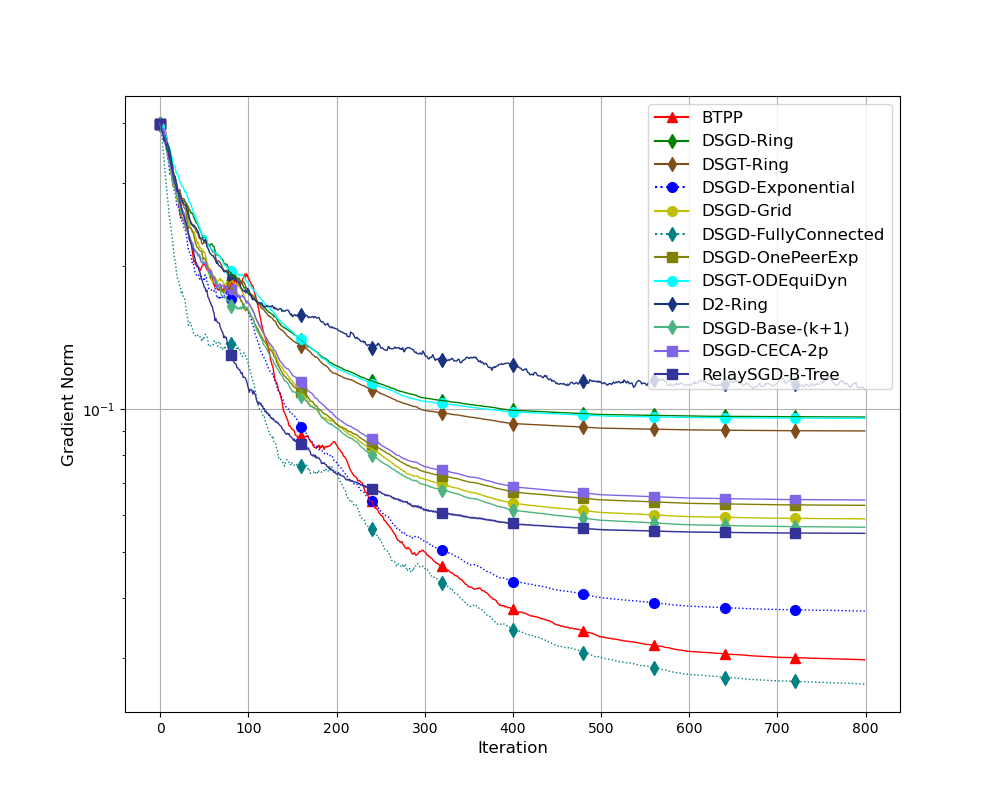
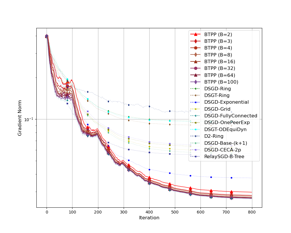
Figure 3: Left: performance of algorithms for logistic regression with nonconvex regularization, where the dotted lines correspond to algorithms whose degrees are not $\Theta(1)$. We let the branch size $B=2$ in BTPP, $\eta=0.5$ in OD-EquiDyn, $k=2$ in Base-($k+1$), and perform RelaySGD on a binary tree graph for fairness. Right: performance of BTPP with different branch size $B$.

4.2 Deep Learning

We apply BTPP and the other algorithms to solve the image classification task with CNN over MNIST dataset [11]. The network contains two convolutional layers with max pooling and ReLu and two feed-forward layers. In particular, we consider a heterogeneous data setting, where data samples are sorted based on their labels and partitioned among the agents. The local batch size is set to $8$ with $24$ agents in total. The learning rate is $0.01$ for all the algorithms except BTPP (which employs a modified stepsize $\gamma/n$) for fairness. Additionally, the starting model is enhanced by pre-training using the SGD optimizer on the entire MNIST dataset for several iterations. Figure 4 illustrates the training loss and the test accuracy curves. Comparing the performance of different algorithms, it can be seen that BTPP (in red) and DSGT with ODEquiDyn (based on $\Theta(n)$ graphs) achieve faster convergence than the other algorithms with $\Theta(1)$ degree and closely approximate the performance of centralized SGD(i.e., DSGD-FullyConnected).

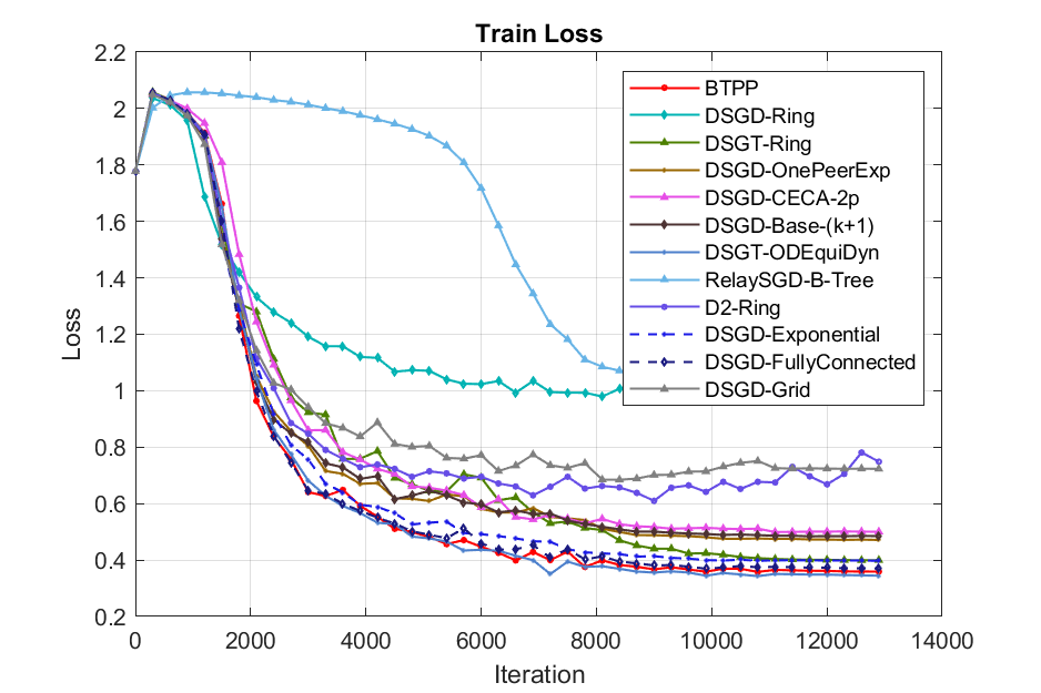
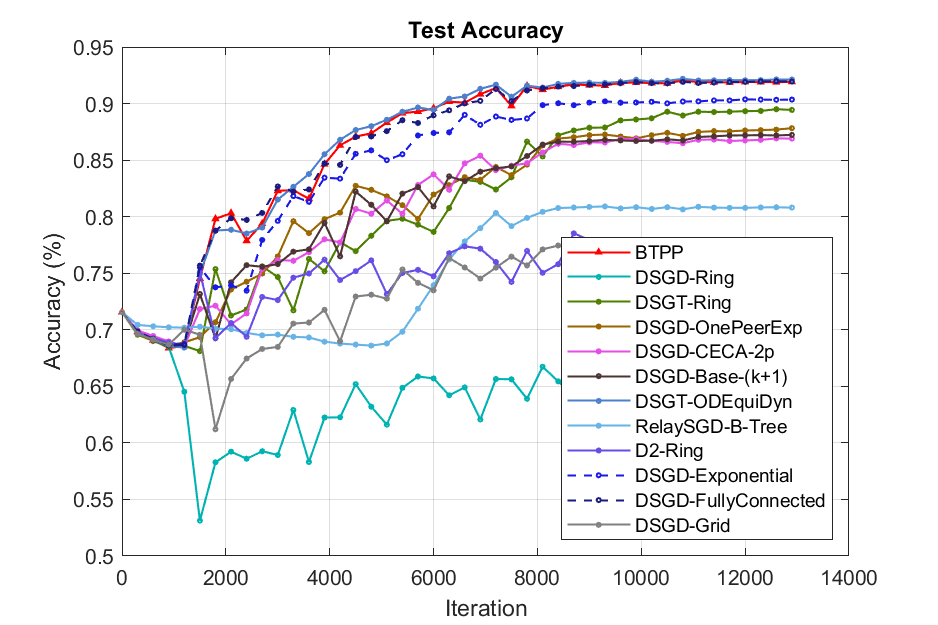
Figure 4: Train loss and test accuracy of different algorithms for training CNN on MNIST, where the dotted lines correspond to the algorithms whose degrees are not $\Theta(1)$. We perform BTPP with $B=2$, ODEquiDyn with $\eta=0.5$, Base-($k+1$) with $k=2$, and RelaySGD on a binary tree graph for fairness.

5 Conclusions

This paper proposes a novel algorithm for distributed learning over heterogeneous data, named BTPP. The convergence is theoretically analyzed for smooth non-convex stochastic optimization. The results demonstrate that, at the minimal communication cost per iteration, BTPP achieves linear speedup in the number of nodes $n$, and the transient times behaves as $\tilde{O}(n)$, outperforming the state-of-the-art results. Numerical experiments further validate the efficiency of BTPP.

Appendix A Convergence Analysis of BTPP

In this section, we aim to demonstrate the convergence results of BTPP through a three-step process. First, we explore the key properties of matrices ${\mathcal{R}}$ and ${\mathcal{C}}$, acquainting readers with several operations that will be frequently utilized in the subsequent parts. Then, we introduce various technical tools essential for the analysis. Finally, we delve into proving the convergence results supported by a series of pertinent lemmas.

A.1 Properties of the Weight Matrices

In this part, we first demonstrate that ${\mathcal{R}}\in\mathbb{R}^{n\times n}$ possesses a set of properties ( the matrix ${\mathcal{C}}={\mathcal{R}}^{{\mathrm{T}}}$ shares similar properties). Then, we utilize the established tools to prove the crucial result presented in Lemma 3.1. Lastly, we provide clarifications on certain matrix operations that will be frequently employed in deriving the convergence results.

It is important to note that for any given $n$ and specific integer $B$, the diameter of the corresponding B-ary tree graph $d$ (the distance from the last layer node to node 1) satisfies $\frac{B^{d}-1}{B-1}<n\leq\frac{B^{d+1}-1}{B-1}$. To investigate the properties of ${\mathcal{R}}$ and ${\mathcal{C}}$, we will introduce the column vector ${\mathbf{e}}_{{\mathcal{I}}}\in\mathbb{R}^{n}$, where each element of ${\mathbf{e}}_{{\mathcal{I}}}$ is equal to 1 for indices $i\in{\mathcal{I}}$ and 0 otherwise. Define the index sets

$${\mathcal{I}}_{1,k} =\left\{1:\frac{B^{k+1}-1}{B-1}\right\},$$

$${\mathcal{I}}_{i,k} =\left\{\left(\frac{B^{k+1}-1}{B-1}+(i-2)B^{k}+1\right):\left(\frac{B^{k+1}-1}{B-1}+(i-1)B^{k}\right)\right\},$$

where $k_{1}:k_{2}$ is the arithmetic progression from $k_{1}$ to $k_{2}$ with difference 1. We can then define the matrix ${\mathbf{Z}}_{k}\in\mathbb{R}^{n\times n}$ as a composite of several column vectors arranged in the following format:

$${\mathbf{Z}}_{k}=\left[{\mathbf{e}}_{{\mathcal{I}}_{1,k}};{\mathbf{e}}_{{\mathcal{I}}_{2,k}};\cdots;{\mathbf{e}}_{{\mathcal{I}}_{n,k}}\right].$$

This closed-form expression of ${\mathcal{R}}$ with any power $k$ is shown in Lemma A.1 which aids in developing further properties.

Lemma A.1.

For the pull matrix $\mathcal{R}$ corresponding to the B-ary tree ${\mathcal{G}}_{{\mathcal{R}}}$, given any positive index $k$, we have

$${\mathcal{R}}^{k}={\mathbf{Z}}_{k}.$$

Proof.

We prove the lemma by induction. First, it is obvious that ${\mathcal{R}}={\mathbf{Z}}_{1}$ by the definition of ${\mathcal{R}}$:

$${\mathcal{R}}_{ij}=1$$

iff $$i\in\{Bj+1-B+[B]\}\cap[n]\text{ or }i=j=1$$

iff $$B(j-1)+2\leq i\leq Bj+1,\ i\in[n]\text{ or }i=j=1$$

iff $$[Z_{1}]_{ij}=1.$$

Now assume the statement is true for $k=j$. Then, for $k=j+1$, we have

$${\mathcal{R}}^{j+1}={\mathcal{R}}^{j}*{\mathcal{R}}={\mathbf{Z}}_{j}{\mathbf{Z}}_{1}.$$

Denote $[{\mathbf{Z}}_{j}\cdot{\mathbf{Z}}_{1}]_{i}$ as the $i$-th column of ${\mathbf{Z}}_{j}\cdot{\mathbf{Z}}_{1}$. To establish the result, we only need to demonstrate that the two matrices, ${\mathcal{R}}^{k+1}$ and ${\mathbf{Z}}_{k+1}$, have the same column entries. For $i=1$,

$${}_{1}={\mathbf{Z}}_{j}[{\mathbf{Z}}_{1}]_{1}=\sum_{i=1}^{B+1}[{\mathbf{Z}}_{j}]_{i}=\sum_{i=1}^{B+1}{\mathbf{e}}_{{\mathcal{I}}_{i,j}}={\mathbf{e}}_{\cup_{i=1}^{B+1}{\mathcal{I}}_{i,j}}={\mathbf{e}}_{{\mathcal{I}}_{1,j+1}}.$$

For $i>1$, we have

$$[{\mathbf{Z}}_{j}{\mathbf{Z}}_{1}]_{i}={\mathbf{Z}}_{j}[{\mathbf{Z}}_{1}]_{i}=\sum_{m\in{\mathcal{I}}_{i,1}}\left[{\mathbf{Z}}_{j}\right]_{m}=\sum_{m=(i-1)B+2}^{iB+1}[{\mathbf{Z}}_{j}]_{m}$$

$$= \sum_{m=(i-1)B}^{iB-1}{\mathbf{e}}_{{\mathcal{I}}_{m,j}}={\mathbf{e}}_{\cup_{m=(i-1)B}^{iB-1}{\mathcal{I}}_{m,j}}={\mathbf{e}}_{{\mathcal{I}}_{i,j+1}}.$$

Thus, we conclude that ${\mathcal{R}}^{k+1}={\mathbf{Z}}_{k+1}$. ∎

Corollary A.2 below reveals that when the power $k$ exceeds $d$, ${\mathcal{R}}^{k}$ transforms into a matrix where the first column is entirely composed of ones, while all the other columns consist of zeros.

Corollary A.2.

For $k=d$, we have

$${\mathcal{R}}^{k}-\frac{1}{n}\mathbbm{1}{\mathbf{u}}^{{\mathrm{T}}}=\mathbf{0}$$

where $\mathbf{0}$ is the matrix with all entries equal 0.

Proof.

From Lemma A.1, we have for the $i$-th column of ${\mathcal{R}}^{k}-\frac{1}{n}\mathbbm{1}{\mathbf{u}}^{{\mathrm{T}}}$ that

$$\left[{\mathcal{R}}^{k}-\frac{1}{n}\mathbbm{1}{\mathbf{u}}^{{\mathrm{T}}}\right]_{i}=\left\{\begin{aligned} -{\mathbf{e}}_{\frac{B^{k+1}-1}{B-1}+1:n}&\ i=1\\ {\mathbf{e}}_{{\mathcal{I}}_{i,k}}&\ i>1\end{aligned}\right.$$

For $k=d$, the first $n$ elements of all the columns remain $0$, which implies the desired result. ∎

Now, we are ready to prove Lemma 3.1:

Proof of Lemma 3.1.

For any integer $k\leq d-1$, define

$$n_{0}:=\left\lfloor\frac{n-\frac{B^{k+1}-1}{B-1}}{B^{k}}\right\rfloor.$$

This ensures that $\frac{B^{k+1}-1}{B-1}+n_{0}B^{k}\leq n$ and $\frac{B^{k+1}-1}{B-1}+(n_{0}+1)B^{k}>n$, so that only the first $(n_{0}+2)$-th columns of ${\mathcal{R}}^{k}$ consist of non-zero elements. Note that

$$\max_{\|{\mathbf{x}}\|_{2}=1}\left\{\|\left({\mathcal{R}}^{k}-\frac{1}{n}\mathbbm{1}{\mathbf{u}}^{{\mathrm{T}}}\right){\mathbf{x}}\|_{2}^{2}\right\}=\max_{{\mathbf{x}}}\left\{\frac{\|\left({\mathcal{R}}^{k}-\frac{1}{n}\mathbbm{1}{\mathbf{u}}^{{\mathrm{T}}}\right){\mathbf{x}}\|_{2}^{2}}{\|{\mathbf{x}}\|^{2}_{2}}\right\}.$$

Then, we focus on the non-zero elements of the matrix ${\mathcal{R}}^{k}-\frac{1}{n}\mathbbm{1}{\mathbf{u}}^{{\mathrm{T}}}$.

$$\frac{\|\left({\mathcal{R}}^{k}-\frac{1}{n}\mathbbm{1}{\mathbf{u}}^{{\mathrm{T}}}\right){\mathbf{x}}\|_{2}^{2}}{\|{\mathbf{x}}\|^{2}_{2}} =\frac{1}{\|{\mathbf{x}}\|^{2}_{2}}\left(\sum_{j=2}^{n_{0}+1}B^{k}(x_{j}-x_{1})^{2}+\left[n-\frac{B^{k+1}-1}{B-1}-B^{k}n_{0}\right]\left(x_{n_{0}+2}-x_{1}\right)^{2}\right)$$

$$:=\frac{\tilde{{\mathbf{x}}}^{{\mathrm{T}}}\Sigma\tilde{{\mathbf{x}}}}{\|{\mathbf{x}}\|^{2}},$$

where $\tilde{{\mathbf{x}}}=\left(x_{1},\cdots,x_{n_{0}+2}\right)$ is the truncated ${\mathbf{x}}$, and

$$\Sigma=\left(\begin{matrix}n-\frac{B^{k+1}-1}{B-1}&-B^{k}&\cdots&-\left[n-\frac{B^{k+1}-1}{B-1}-B^{k}n_{0}\right]\\ -B^{k}&B^{k}&&\\ \vdots&&\ddots&\\ -\left[n-\frac{B^{k+1}-1}{B-1}-B^{k}n_{0}\right]&&&\left[n-\frac{B^{k+1}-1}{B-1}-B^{k}n_{0}\right]\end{matrix}\right),$$

where the unspecified elements are all zeros. Since $\Sigma$ is symmetric, all the eigenvalues are real. We show by contradiction that any eigenvalue $\lambda$ of $\Sigma$ is upper bounded by $n$. Otherwise, if there exists $\lambda>n$, we denote ${\mathbf{x}}$ as the corresponding eigenvector of $\lambda$. Then, we have from $\Sigma{\mathbf{x}}=\lambda{\mathbf{x}}$ that

$$\lambda x_{1} =\left(n-\frac{B^{k+1}-1}{B-1}\right)x_{1}-B^{k}x_{2}-\cdots-\left[n-\frac{B^{k+1}-1}{B-1}-B^{k}n_{0}\right]x_{n_{0}+2}$$

$$\lambda x_{2} =-B^{k}x_{1}+B^{k}x_{2}$$

$$\lambda x_{3} =-B^{k}x_{1}+B^{k}x_{3}$$

$$\cdots$$

$$\lambda x_{n_{0}+2} =-\left[n-\frac{B^{k+1}-1}{B-1}-B^{k}n_{0}\right]x_{1}+\left[n-\frac{B^{k+1}-1}{B-1}-B^{k}n_{0}\right]x_{n_{0}+2}.$$

Without loss of generality, assume $x_{1}\neq 0$. Then, by substituting the other relations into the first one, we have

$$\lambda=n-\frac{B^{k+1}-1}{B-1}+\sum_{i=1}^{n_{0}}\frac{B^{2k}}{\lambda-B^{k}}+\frac{\left[n-\frac{B^{k+1}-1}{B-1}-B^{k}n_{0}\right]^{2}}{\lambda-\left[n-\frac{B^{k+1}-1}{B-1}-B^{k}n_{0}\right]}.$$

With the fact that $\lambda>n$, there holds

$$\lambda\leq n-\frac{B^{k+1}-1}{B-1}+\frac{n_{0}B^{2k}}{n-B^{k}}+\frac{\left[n-\frac{B^{k+1}-1}{B-1}-B^{k}n_{0}\right]^{2}}{n-\left[n-\frac{B^{k+1}-1}{B-1}-B^{k}n_{0}\right]}$$

$$= n-\frac{B^{k+1}-1}{B-1}+\frac{n_{0}B^{2k}}{n-B^{k}}+\frac{n^{2}}{\frac{B^{k+1}-1}{B-1}+B^{k}n_{0}}-2n+\frac{B^{k+1}-1}{B-1}+B^{k}n_{0}$$

$$= \frac{nB^{k}n_{0}}{n-B^{k}}+\frac{n\left(n-\frac{B^{k+1}-1}{B-1}-B^{k}n_{0}\right)}{\frac{B^{k+1}-1}{B-1}+B^{k}n_{0}}$$

$$\leq \frac{nB^{k}n_{0}}{n-B^{k}}+\frac{n}{n-B^{k}}\left(n-\frac{B^{k+1}-1}{B-1}-B^{k}n_{0}\right)$$

$$= n\frac{n-\frac{B^{k+1}-1}{B-1}}{n-B^{k}}<n,$$

which is a contradiction. Thus, we have $\lambda\leq n$. It follows that

$$\frac{\tilde{{\mathbf{x}}}^{{\mathrm{T}}}\Sigma\tilde{{\mathbf{x}}}}{\|{\mathbf{x}}\|^{2}}\leq\frac{\tilde{{\mathbf{x}}}^{{\mathrm{T}}}\Sigma\tilde{{\mathbf{x}}}}{\|\tilde{{\mathbf{x}}}\|^{2}}\leq\lambda_{\max}(\Sigma)\leq n.$$

From the fact that the square root function is monotonically increasing on $[0,\infty)$, we have

$$\|{\mathcal{R}}^{k}-\frac{1}{n}\mathbbm{1}{\mathbf{u}}^{{\mathrm{T}}}\|_{2}^{2}=\max_{\|{\mathbf{x}}\|_{2}=1}\left\{\|\left({\mathcal{R}}^{k}-\frac{1}{n}\mathbbm{1}{\mathbf{u}}^{{\mathrm{T}}}\right){\mathbf{x}}\|_{2}^{2}\right\}\leq n,$$

which implies that $\|{\mathcal{R}}^{k}-\frac{1}{n}\mathbbm{1}{\mathbf{u}}^{{\mathrm{T}}}\|_{2}\leq\sqrt{n}$ for $k\leq d-1$ and $\|{\mathcal{R}}^{k}-\frac{1}{n}\mathbbm{1}{\mathbf{u}}^{{\mathrm{T}}}\|_{2}=0$ otherwise by Corollary A.2. ∎

The transformations described in Corollary A.3 below are straightforward.

Corollary A.3.

For any integer $m>0$, we have

$${\bm{\Pi}}_{{\mathbf{u}}}{\mathcal{R}} ={\bm{\Pi}}_{{\mathbf{u}}}\left({\mathcal{R}}-\frac{1}{n}\mathbbm{1}{\mathbf{u}}^{{\mathrm{T}}}\right)=\left({\mathcal{R}}-\frac{1}{n}\mathbbm{1}{\mathbf{u}}^{{\mathrm{T}}}\right){\bm{\Pi}}_{{\mathbf{u}}},$$

$${\bm{\Pi}}_{{\mathbf{u}}}{\mathcal{R}}^{m} ={\bm{\Pi}}_{{\mathbf{u}}}\left({\mathcal{R}}^{m}-\frac{1}{n}\mathbbm{1}{\mathbf{u}}^{{\mathrm{T}}}\right)={\bm{\Pi}}_{{\mathbf{u}}}\left({\mathcal{R}}-\frac{1}{n}\mathbbm{1}{\mathbf{u}}^{{\mathrm{T}}}\right)^{m}=\left({\mathcal{R}}-\frac{1}{n}\mathbbm{1}{\mathbf{u}}^{{\mathrm{T}}}\right)^{m}{\bm{\Pi}}_{{\mathbf{u}}}.$$

To simplify the convergence analysis, we introduce the matrix ${\mathbf{A}}_{i}$ defined as follows:

$${\mathbf{A}}_{i}={\mathcal{C}}^{i}-{\mathcal{C}}^{i-1}$$

for $i=1,2,\cdots,d$. Specifically, ${\mathbf{A}}_{1}={\mathcal{C}}-{\mathbf{I}}$. Consequently, Corollary A.4 below can be directly deduced from Lemma A.1 and Corollary A.3.

Corollary A.4.

For $i=1,\cdots,d$, we have

$$\left(\frac{{\mathbf{u}}^{{\mathrm{T}}}}{n}-\mathbbm{1}^{{\mathrm{T}}}\right){\mathbf{A}}_{i}=\left\{\begin{aligned} {\mathbf{e}}_{\frac{B^{i}-1}{B-1}+1:\frac{B^{i+1}-1}{B-1}}^{{\mathrm{T}}}&\quad i\leq d-1\\ {\mathbf{e}}_{\frac{B^{d}-1}{B-1}+1:n}^{{\mathrm{T}}}&\quad i=d\end{aligned}\right.$$

Intuitively, Corollary A.4 illustrates that $\left(\frac{{\mathbf{u}}^{{\mathrm{T}}}}{n}-\mathbbm{1}^{{\mathrm{T}}}\right){\mathbf{A}}_{i}$ serves as an indicator vector representing the $(i+1)$-th layer of the graph.

A.2 Supporting Inequalities and Lemmas

Lemma A.5 and Lemma A.6 below are frequently employed for bounding the norms of matrix summations and multiplications. Their proofs rely on the Cauchy-Schwartz inequality and the definitions of matrix norms $\|\cdot\|_{2}$ and $\|\cdot\|_{F}$.

Lemma A.5.

For an arbitrary set of $m$ matrices $\{{\mathbf{A}}_{i}\}_{i=1}^{m}$ with the same size, we have

$$\left\|\sum_{i=1}^{m}{\mathbf{A}}_{i}\right\|_{F}^{2}\leq m\sum_{i=1}^{m}\left\|{\mathbf{A}}_{i}\right\|_{F}^{2}.$$

Proof.

By the definition of Frobenius norm, we have

$$\left\|\sum_{i=1}^{m}{\mathbf{A}}_{i}\right\|_{F}\leq\sum_{i=1}^{m}\left\|{\mathbf{A}}_{i}\right\|_{F}.$$

Taking squares on both sides and invoking the Cauchy-Schwarz inequality, we have

$$\left\|\sum_{i=1}^{m}{\mathbf{A}}_{i}\right\|_{F}^{2}\leq\left(\sum_{i=1}^{m}\left\|{\mathbf{A}}_{i}\right\|_{F}\right)^{2}\leq m\sum_{i=1}^{m}\left\|{\mathbf{A}}_{i}\right\|_{F}^{2}.$$

∎

Lemma A.6.

Let ${\mathbf{A}}$, ${\mathbf{B}}$ be two real matrices whose sizes match. Then,

$$\left\|{\mathbf{A}}{\mathbf{B}}\right\|_{F}\leq\left\|{\mathbf{A}}\right\|_{2}\left\|{\mathbf{B}}\right\|_{F}.$$

Proof.

Let ${\mathbf{A}}={\mathbf{U}}\Sigma{\mathbf{V}}^{H}$ be the singular value decomposition of ${\mathbf{A}}$, with the largest singular value $\sigma_{\max}$ and hence $\left\|{\mathbf{A}}\right\|_{2}=\sigma_{\max}$. Then, we have

$$\left\|{\mathbf{A}}{\mathbf{B}}\right\|_{F}^{2} =\left\|{\mathbf{U}}\Sigma{\mathbf{V}}^{H}{\mathbf{B}}\right\|_{F}^{2}=\text{trace}\left(\left({\mathbf{U}}\Sigma{\mathbf{V}}^{H}{\mathbf{B}}\right)^{H}\left({\mathbf{U}}\Sigma{\mathbf{V}}^{H}{\mathbf{B}}\right)\right)$$

$$=\text{trace}\left(\left(\Sigma{\mathbf{V}}^{H}{\mathbf{B}}\right)^{H}\left(\Sigma{\mathbf{V}}^{H}{\mathbf{B}}\right)\right)=\left\|\Sigma{\mathbf{V}}^{H}{\mathbf{B}}\right\|_{F}^{2}$$

$$\leq\sigma_{\max}^{2}\|{\mathbf{V}}^{H}{\mathbf{B}}\|_{F}^{2}=\sigma_{\max}^{2}\text{trace}\left({\mathbf{B}}^{{\mathrm{T}}}{\mathbf{V}}{\mathbf{V}}^{H}{\mathbf{B}}\right)$$

$$=\sigma_{\max}^{2}\text{trace}\left({\mathbf{B}}^{{\mathrm{T}}}{\mathbf{B}}\right)=\sigma_{\max}^{2}\left\|{\mathbf{B}}\right\|_{F}^{2}$$

$$=\left\|{\mathbf{A}}\right\|_{2}^{2}\left\|{\mathbf{B}}\right\|_{F}^{2},$$

which implies the desired result. ∎

Lemma A.7 below will be used in the last step for deriving the convergence rate of BTPP.

Lemma A.7.

Let $A,B,C$ and $\alpha$ be positive constants and $T$ be a positive integer. Define function

$$g(\gamma)=\frac{A}{\gamma(T+1)}+B\gamma+C\gamma^{2}.$$

Then,

$$\inf_{\gamma\in(0,\frac{1}{\alpha}]}g(\gamma)\leq 2\left(\frac{AB}{T+1}\right)^{\frac{1}{2}}+2C^{\frac{1}{3}}\left(\frac{A}{T+1}\right)^{\frac{2}{3}}+\frac{\alpha A}{T+1},$$

where the upper bound can be achieved by choosing $\gamma=\min\left\{\left(\frac{A}{B(T+1)}\right)^{\frac{1}{2}},\left(\frac{A}{C(T+1)}\right)^{\frac{1}{3}},\frac{1}{\alpha}\right\}$.

Proof.

See Lemma 26 in [8] for a reference. ∎

Lemma A.8 is a technical result related to random variables.

Lemma A.8.

Consider three random variables $X$, $Y$, and $Z$. Assume that $Z$ is independent with $(X,Y)$. Let $h$ and $g$ be functions such that the conditional expectation $\mathbb{E}[g(Y,Z)\mid Y]=0$. We have

$$\mathbb{E}\left(h(X)g(Y,Z)\right)=0.$$

Proof.

It implies by the condition $Z\perp\!\!\!\perp(X,Y)$ that $\sigma(Z)\perp\!\!\!\perp\sigma(X,Y)$. Then,

$$\mathbb{E}\left[h(X)g(Y,Z)|Y\right] =\mathbb{E}\left\{\mathbb{E}\left[h(X)g(Y,Z)|X,Y\right]|Y\right\}$$

$$=\mathbb{E}\left\{h(X)\mathbb{E}\left[g(Y,Z)|X,Y\right]|Y\right\}.$$

It suffices to show

$$\mathbb{E}\left[g(Y,Z)|X,Y\right]=\mathbb{E}\left[g(Y,Z)|Y\right](=0).$$

Let $f_{g}(y)=\mathbb{E}\left(g(y,Z)\right)$. Since $\sigma(Z)\perp\!\!\!\perp\sigma(X,Y)$, we have $\sigma(Z)\perp\!\!\!\perp\sigma(Y)$. Then,

$$f_{g}(Y)=\mathbb{E}\left(g(Y,Z)|Y\right)=\mathbb{E}\left[g(Y,Z)|X,Y\right],$$

which follows directly from (10.17) in [24]. Thus, by the Tower Rule, we reach the statement as follows:

$$\mathbb{E}\left(h(X)g(Y,Z)\right)=\mathbb{E}\left\{\mathbb{E}\left(h(X)g(Y,Z)|Y\right)\right\}=0.$$

∎

A.3 Proofs of Key Lemmas

In this section, we prove several key lemmas for proving the main convergence result of BTPP.

A.3.1 Preparation

Algorithm 1, as encapsulated by the equations in (2), can be succinctly expressed in the following matrix form:

$$\left(\begin{array}[]{c}{\mathbf{X}}^{(t+1)}\\ {\mathbf{Y}}^{(t+1)}\end{array}\right)=\left(\begin{array}[]{cc}{\mathcal{R}}&-\gamma{\mathcal{R}}\\ \mathbf{0}&{\mathcal{C}}\end{array}\right)\left(\begin{array}[]{c}{\mathbf{X}}^{(t)}\\ {\mathbf{Y}}^{(t)}\end{array}\right)+\left(\begin{array}[]{c}\mathbf{0}\\ {\mathbf{G}}^{(t+1)}-{\mathbf{G}}^{(t)}\end{array}\right).$$ (4)

By repeatedly applying equation (4) starting from time step $t$ and going back to time step $0$, we arrive at the following relation:

$$\left(\begin{array}[]{c}{\mathbf{X}}^{(t)}\\ {\mathbf{Y}}^{(t)}\end{array}\right) =\left(\begin{array}[]{cc}{\mathcal{R}}&-\gamma{\mathcal{R}}\\ \mathbf{0}&{\mathcal{C}}\end{array}\right)^{t}\left(\begin{array}[]{c}{\mathbf{X}}^{(0)}\\ {\mathbf{Y}}^{(0)}\end{array}\right)+\sum_{m=0}^{t-1}\left(\begin{array}[]{cc}{\mathcal{R}}&-\gamma{\mathcal{R}}\\ \mathbf{0}&{\mathcal{C}}\end{array}\right)^{t-m-1}\left(\begin{array}[]{c}\mathbf{0}\\ {\mathbf{G}}^{(m+1)}-{\mathbf{G}}^{(m)}\end{array}\right).$$

For the sake of clarity, we start with introducing some simple definitions. Any matrix raised to the power of 0 is defined as the identity matrix ${\mathbf{I}}$, which matches the original matrix in dimension. The only exceptions are $\left({\mathcal{R}}-\frac{1}{n}\mathbbm{1}{\mathbf{u}}^{{\mathrm{T}}}\right)^{0}:={\bm{\Pi}}_{{\mathbf{u}}}$ and $\left({\mathcal{C}}-\frac{1}{n}{\mathbf{v}}\mathbbm{1}^{{\mathrm{T}}}\right)^{0}:={\bm{\Pi}}_{{\mathbf{v}}}$ for convenience. Furthermore, we introduce the following terms:

$$\bar{{\mathbf{X}}}^{(t)}:=\frac{1}{n}\mathbbm{1}{\mathbf{u}}^{{\mathrm{T}}}{\mathbf{X}}^{(t)},\ \bar{{\mathbf{Y}}}^{(t)}:=\frac{1}{n}{\mathbf{v}}\mathbbm{1}^{{\mathrm{T}}}{\mathbf{Y}}^{(t)}.$$

Note that, for any given integer $m>0$,

$$\left(\begin{array}[]{cc}{\mathcal{R}}&-\gamma{\mathcal{R}}\\ \mathbf{0}&{\mathcal{C}}\end{array}\right)^{m}=\left(\begin{array}[]{cc}{\mathcal{R}}^{m}&-\gamma\sum_{j=1}^{m}{\mathcal{R}}^{j}{\mathcal{C}}^{m-j}\\ \mathbf{0}&{\mathcal{C}}^{m}\end{array}\right).$$

As a result, given the initial condition ${\mathbf{Y}}^{(0)}={\mathbf{G}}^{(0)}$, we can deduce the outcomes of ${\mathbf{X}}^{(t)}$ and ${\mathbf{Y}}^{(t)}$ as follows.

$${\mathbf{X}}^{(t)} ={\mathcal{R}}^{t}{\mathbf{X}}^{(0)}-\gamma\sum_{m=0}^{t-2}\sum_{j=1}^{t-m-1}{\mathcal{R}}^{j}{\mathcal{C}}^{t-m-1-j}\left[{\mathbf{G}}^{(m+1)}-{\mathbf{G}}^{(m)}\right]-\gamma\sum_{j=1}^{t}{\mathcal{R}}^{j}{\mathcal{C}}^{t-j}{\mathbf{G}}^{(0)},$$ (5)

$${\mathbf{Y}}^{(t)} =\sum_{m=0}^{t-1}{\mathcal{C}}^{t-m-1}\left[{\mathbf{G}}^{(m+1)}-{\mathbf{G}}^{(m)}\right]+{\mathcal{C}}^{t}{\mathbf{G}}^{(0)}.$$ (6)

Then, after multiplying ${\bm{\Pi}}_{{\mathbf{u}}}$ and ${\bm{\Pi}}_{{\mathbf{v}}}$ to equation (5) and equation (6) respectively, and invoking Corollary A.3, we have

$$\begin{split}{\bm{\Pi}}_{{\mathbf{u}}}{\mathbf{X}}^{(t)}&=\left({\mathcal{R}}-\frac{1}{n}\mathbbm{1}{\mathbf{u}}^{{\mathrm{T}}}\right)^{t}{\mathbf{X}}^{(0)}-\gamma\sum_{j=1}^{\min\left\{d-1,t\right\}}\left({\mathcal{R}}-\frac{1}{n}\mathbbm{1}{\mathbf{u}}^{{\mathrm{T}}}\right)^{j}{\mathcal{C}}^{t-j}{\mathbf{G}}^{(0)}\\ &\quad-\gamma\sum_{m=0}^{t-2}\sum_{j=1}^{\min\left\{t-m-1,d-1\right\}}\left({\mathcal{R}}-\frac{1}{n}\mathbbm{1}{\mathbf{u}}^{{\mathrm{T}}}\right)^{j}{\mathcal{C}}^{t-m-1-j}\left[{\mathbf{G}}^{(m+1)}-{\mathbf{G}}^{(m)}\right],\end{split}$$ (7)

$$\begin{split}{\bm{\Pi}}_{{\mathbf{v}}}{\mathbf{Y}}^{(t)}&=\sum_{m=\max\left\{0,t-d\right\}}^{t-1}\left({\mathcal{C}}-\frac{1}{n}{\mathbf{v}}\mathbbm{1}^{{\mathrm{T}}}\right)^{t-m-1}\left[{\mathbf{G}}^{(m+1)}-{\mathbf{G}}^{(m)}\right]+\left({\mathcal{C}}-\frac{1}{n}{\mathbf{v}}\mathbbm{1}^{{\mathrm{T}}}\right)^{t}{\mathbf{G}}^{(0)}\\ &=\sum_{m=0}^{\min\{t,d\}-1}\left({\mathcal{C}}-\frac{1}{n}{\mathbf{v}}\mathbbm{1}^{{\mathrm{T}}}\right)^{m}\left({\mathbf{G}}^{(t-m)}-{\mathbf{G}}^{(t-m-1)}\right)+\left({\mathcal{C}}-\frac{1}{n}{\mathbf{v}}\mathbbm{1}^{{\mathrm{T}}}\right)^{t}{\mathbf{G}}^{(0)}\\ &=\sum_{m=1}^{\min\{t,d\}}{\mathbf{A}}_{m}{\mathbf{G}}^{(t-m)}+{\bm{\Pi}}_{{\mathbf{v}}}{\mathbf{G}}^{(t)}.\end{split}$$ (8)

A.3.2 Proof of Lemma 3.2

Proof.

For any given $t$ and $i\neq j$, due to the independently drawn sample $\xi_{i}^{(t)}$, we have that $\xi_{i}^{(t)}$ is independent of $({\mathcal{F}}_{t},\xi_{j}^{(t)})$, and thus $\xi_{i}^{(t)}$ is independent of $\sigma(x_{i}^{(t)},x_{j}^{(t)},\xi_{j}^{(t)})$. Hence, invoking Lemma A.8 and 1.1 yields

$$\mathbb{E}\left[\nabla F(x_{i}^{(t)};\xi_{i}^{(t)})-\nabla f_{i}(x_{i}^{(t)})\bigg{|}x_{i}^{(t)}\right]=\mathbb{E}\left[\nabla F(x_{i}^{(t)};\xi_{i}^{(t)})-\nabla f_{i}(x_{i}^{(t)})\bigg{|}{\mathcal{F}}_{t}\right]=0,$$

$$\mathbb{E}\left\langle\nabla F(x_{i}^{(t)};\xi_{i}^{(t)})-\nabla f_{i}(x_{i}^{(t)}),\nabla F(x_{j}^{(t)};\xi_{j}^{(t)})-\nabla f_{j}(x_{j}^{(t)})\right\rangle=0.$$

Then, for any index set ${\mathcal{I}}\subseteq\{1,2,\cdots,n\}$, we have $\mathbb{E}\|{\mathbf{e}}_{{\mathcal{I}}}^{{\mathrm{T}}}\left({\mathbf{G}}^{(t)}-\nabla{\mathbf{F}}({\mathbf{X}}^{(t)})\right)\|_{2}^{2}\leq|{\mathcal{I}}|\sigma^{2}$.

Notice that

$$\left\|\left({\mathcal{C}}-\frac{1}{n}{\mathbf{v}}\mathbbm{1}^{{\mathrm{T}}}\right)^{k}\left({\mathbf{G}}^{(t)}-\nabla{\mathbf{F}}({\mathbf{X}}^{(t)})\right)\right\|_{F}^{2}= \left\|{\mathbf{e}}_{\frac{B^{k+1}-1}{B-1}+1:n}\left({\mathbf{G}}^{(t)}-\nabla{\mathbf{F}}({\mathbf{X}}^{(t)})\right)\right\|_{2}^{2}$$

$$+\sum_{i=2}^{n}\left\|{\mathbf{e}}_{{\mathcal{I}}_{i,k}}\left({\mathbf{G}}^{(t)}-\nabla{\mathbf{F}}({\mathbf{X}}^{(t)})\right)\right\|_{2}^{2}.$$

Thus, we obtain the desired result by invoking Lemma A.1 and Corollary A.2 after taking expectation on both sides of the above relation:

$$\mathbb{E}\left\|\left({\mathcal{C}}-\frac{1}{n}{\mathbf{v}}\mathbbm{1}^{{\mathrm{T}}}\right)^{j}\left({\mathbf{G}}^{(t)}-\nabla{\mathbf{F}}({\mathbf{X}}^{(t)})\right)\right\|_{F}^{2}\leq 2\left(n-\frac{B^{k+1}-1}{B-1}\right)\sigma^{2}\leq 2n\sigma^{2}.$$

∎

Under 1.1 and the randomly selected samples, Lemma 3.2 and Corollary A.9 below provide an initial estimation for the variance terms. The proof of Corollary A.9 is directly from the analysis in subsection A.3.2 and Corollary A.4.

Corollary A.9.

Under 1.1, we have for all $t\geq 0$ that

$$\sum_{k=1}^{d}\mathbb{E}\|\left(\frac{{\mathbf{u}}^{{\mathrm{T}}}}{n}-\mathbbm{1}^{{\mathrm{T}}}\right)A_{k}\left({\mathbf{G}}({\mathbf{X}}^{(t)},{\bm{\xi}}^{(t)})-\nabla{\mathbf{F}}({\mathbf{X}}^{(t)})\right)\|_{2}^{2}\leq(n-1)\sigma^{2}.$$

A.3.3 Proof of Lemma 3.3

Proof.

Notice that

$$\bar{{\mathbf{X}}}^{(t+1)}-\bar{{\mathbf{X}}}^{(t)}=-\gamma\frac{1}{n}\mathbbm{1}{\mathbf{u}}^{{\mathrm{T}}}{\mathbf{Y}}^{(t)}=-\gamma\frac{1}{n}\mathbbm{1}{\mathbf{u}}^{{\mathrm{T}}}\left[{\bm{\Pi}}_{{\mathbf{v}}}{\mathbf{Y}}^{(t)}+\frac{1}{n}{\mathbf{v}}\mathbbm{1}^{{\mathrm{T}}}{\mathbf{Y}}^{(t)}\right]$$

$$\qquad=-\gamma\frac{1}{n}\mathbbm{1}{\mathbf{u}}^{{\mathrm{T}}}{\bm{\Pi}}_{{\mathbf{v}}}{\mathbf{Y}}^{(t)}-\gamma\mathbbm{1}\mathbbm{1}^{{\mathrm{T}}}{\mathbf{Y}}^{(t)}=-\gamma\mathbbm{1}\left(\frac{{\mathbf{u}}^{{\mathrm{T}}}}{n}-\mathbbm{1}^{{\mathrm{T}}}\right){\bm{\Pi}}_{{\mathbf{v}}}{\mathbf{Y}}^{(t)}-\gamma\mathbbm{1}\mathbbm{1}^{{\mathrm{T}}}{\mathbf{Y}}^{(t)}.$$

Multiplying $\mathbbm{1}^{{\mathrm{T}}}$ on both sides of equation (6), we have $\mathbbm{1}^{{\mathrm{T}}}{\mathbf{Y}}^{(t)}=\mathbbm{1}^{{\mathrm{T}}}{\mathbf{G}}^{(t)}$ for any integer $t$. Thus, in light of equation (8), we have

$$\bar{{\mathbf{X}}}^{(t+1)}-\bar{{\mathbf{X}}}^{(t)}=-\gamma\mathbbm{1}\left(\frac{{\mathbf{u}}^{{\mathrm{T}}}}{n}-\mathbbm{1}^{{\mathrm{T}}}\right){\bm{\Pi}}_{{\mathbf{v}}}{\mathbf{Y}}^{(t)}-\gamma\mathbbm{1}\mathbbm{1}^{{\mathrm{T}}}{\mathbf{G}}^{(t)}$$

$$\qquad=-\gamma\mathbbm{1}\left(\frac{{\mathbf{u}}^{{\mathrm{T}}}}{n}-\mathbbm{1}^{{\mathrm{T}}}\right)\sum_{m=1}^{\min\left\{t,d\right\}}{\mathbf{A}}_{m}{\mathbf{G}}^{(t-m)}-\gamma\mathbbm{1}\left(\frac{{\mathbf{u}}^{{\mathrm{T}}}}{n}-\mathbbm{1}^{{\mathrm{T}}}\right){\mathbf{G}}^{(t)}-\gamma\mathbbm{1}\mathbbm{1}^{{\mathrm{T}}}{\mathbf{G}}^{(t)}$$

$$\qquad=-\gamma\mathbbm{1}\left(\frac{{\mathbf{u}}^{{\mathrm{T}}}}{n}-\mathbbm{1}^{{\mathrm{T}}}\right)\sum_{m=1}^{\min\left\{t,d\right\}}{\mathbf{A}}_{m}\left({\mathbf{G}}^{(t-m)}-\nabla{\mathbf{F}}({\mathbf{X}}^{(t-m)})\right)$$

$$\qquad\qquad-\gamma\mathbbm{1}\left(\frac{{\mathbf{u}}^{{\mathrm{T}}}}{n}-\mathbbm{1}^{{\mathrm{T}}}\right)\sum_{m=1}^{\min\left\{t,d\right\}}{\mathbf{A}}_{m}\nabla{\mathbf{F}}({\mathbf{X}}^{(t-m)})-\gamma\mathbbm{1}\frac{{\mathbf{u}}^{{\mathrm{T}}}}{n}{\mathbf{G}}^{(t)}$$

$$\qquad=-\gamma\mathbbm{1}\left(\frac{{\mathbf{u}}^{{\mathrm{T}}}}{n}-\mathbbm{1}^{{\mathrm{T}}}\right)\sum_{m=1}^{\min\left\{t,d\right\}}{\mathbf{A}}_{m}\left({\mathbf{G}}^{(t-m)}-\nabla{\mathbf{F}}({\mathbf{X}}^{(t-m)})\right)$$

$$\qquad\qquad-\gamma\mathbbm{1}\left(\frac{{\mathbf{u}}^{{\mathrm{T}}}}{n}-\mathbbm{1}^{{\mathrm{T}}}\right)\sum_{m=\max\{0,t-d\}}^{t-1}\left({\mathcal{C}}-\frac{1}{n}{\mathbf{v}}\mathbbm{1}^{{\mathrm{T}}}\right)^{t-m-1}\left[\nabla{\mathbf{F}}({\mathbf{X}}^{(m+1)})-\nabla{\mathbf{F}}({\mathbf{X}}^{(m)})\right]$$

$$\qquad\qquad-\gamma\mathbbm{1}\left(\frac{{\mathbf{u}}^{{\mathrm{T}}}}{n}-\mathbbm{1}^{{\mathrm{T}}}\right)\left({\mathcal{C}}-\frac{1}{n}{\mathbf{v}}\mathbbm{1}^{{\mathrm{T}}}\right)^{t}\nabla{\mathbf{F}}({\mathbf{X}}^{(0)})+\gamma\mathbbm{1}\left(\frac{{\mathbf{u}}^{{\mathrm{T}}}}{n}-\mathbbm{1}^{{\mathrm{T}}}\right)\nabla{\mathbf{F}}({\mathbf{X}}^{(t)})-\gamma\mathbbm{1}\frac{{\mathbf{u}}^{{\mathrm{T}}}}{n}{\mathbf{G}}^{(t)}.$$

Hence, taking the F-norm and expectation on both sides, we have from Lemma A.5 that

$$\mathbb{E}\|\bar{{\mathbf{X}}}^{(t+1)}-\bar{{\mathbf{X}}}^{(t)}\|_{F}^{2}\leq 5\gamma^{2}n\mathbb{E}\left\|\sum_{m=1}^{\min\left\{t,d\right\}}\left(\frac{{\mathbf{u}}^{{\mathrm{T}}}}{n}-\mathbbm{1}^{{\mathrm{T}}}\right){\mathbf{A}}_{m}\left({\mathbf{G}}^{(t-m)}-\nabla{\mathbf{F}}({\mathbf{X}}^{(t-m)})\right)\right\|_{F}^{2}$$ (9)

$$\qquad+5\gamma^{2}n\mathbb{E}\left\|\left(\frac{{\mathbf{u}}^{{\mathrm{T}}}}{n}-\mathbbm{1}^{{\mathrm{T}}}\right)\sum_{m=\max\{0,t-d\}}^{t-1}\left({\mathcal{C}}-\frac{1}{n}{\mathbf{v}}\mathbbm{1}^{{\mathrm{T}}}\right)^{t-m-1}\left[\nabla{\mathbf{F}}({\mathbf{X}}^{(m+1)})-\nabla{\mathbf{F}}({\mathbf{X}}^{(m)})\right]\right\|_{F}^{2}$$

$$\qquad+5\gamma^{2}n\mathbb{E}\left\|\left(\frac{{\mathbf{u}}^{{\mathrm{T}}}}{n}-\mathbbm{1}^{{\mathrm{T}}}\right)\left({\mathcal{C}}-\frac{1}{n}{\mathbf{v}}\mathbbm{1}^{{\mathrm{T}}}\right)^{{\mathrm{T}}}\nabla{\mathbf{F}}({\mathbf{X}}^{(0)})\right\|_{F}^{2}$$

$$\qquad+5\gamma^{2}n\mathbb{E}\left\|\frac{{\mathbf{u}}^{{\mathrm{T}}}}{n}\left(\nabla{\mathbf{F}}({\mathbf{X}}^{(t)})-{\mathbf{G}}^{(t)}\right)\right\|_{F}^{2}+5\gamma^{2}n\mathbb{E}\left\|\mathbbm{1}^{{\mathrm{T}}}{\mathbf{F}}({\mathbf{X}}^{(t)})\right\|_{F}^{2}.$$

Note that, invoking Lemma 3.2 and Corollary A.9 yields

$$\mathbb{E}\left\|\sum_{m=1}^{\min\left\{t,d\right\}}\left(\frac{{\mathbf{u}}^{{\mathrm{T}}}}{n}-\mathbbm{1}^{{\mathrm{T}}}\right){\mathbf{A}}_{m}\left({\mathbf{G}}^{(t-m)}-\nabla{\mathbf{F}}({\mathbf{X}}^{(t-m)})\right)\right\|_{F}^{2}$$

$$= \sum_{m=1}^{\min\left\{t,d\right\}}\mathbb{E}\left\|\left(\frac{{\mathbf{u}}^{{\mathrm{T}}}}{n}-\mathbbm{1}^{{\mathrm{T}}}\right){\mathbf{A}}_{m}\left({\mathbf{G}}^{(t-m)}-\nabla{\mathbf{F}}({\mathbf{X}}^{(t-m)})\right)\right\|_{F}^{2}$$

$$\leq (n-1)\sigma^{2}.$$

From 1.2, Lemma A.6 and Lemma A.5, we have

$$\mathbb{E}\left\|\left(\frac{{\mathbf{u}}^{{\mathrm{T}}}}{n}-\mathbbm{1}^{{\mathrm{T}}}\right)\sum_{m=\max\{0,t-d\}}^{t-1}\left({\mathcal{C}}-\frac{1}{n}{\mathbf{v}}\mathbbm{1}^{{\mathrm{T}}}\right)^{t-m-1}\left[\nabla{\mathbf{F}}({\mathbf{X}}^{(m+1)})-\nabla{\mathbf{F}}({\mathbf{X}}^{(m)})\right]\right\|_{F}^{2}$$

$$\leq d\sum_{m=\max\{0,t-d\}}^{t-1}\mathbb{E}\left\|\left(\frac{{\mathbf{u}}^{{\mathrm{T}}}}{n}-\mathbbm{1}^{{\mathrm{T}}}\right)\left({\mathcal{C}}-\frac{1}{n}{\mathbf{v}}\mathbbm{1}^{{\mathrm{T}}}\right)^{t-m-1}\left[\nabla{\mathbf{F}}({\mathbf{X}}^{(m+1)})-\nabla{\mathbf{F}}({\mathbf{X}}^{(m)})\right]\right\|_{F}^{2}$$

$$\leq d\sum_{m=\max\{0,t-d\}}^{t-1}\mathbb{E}\left\|\left(\frac{{\mathbf{u}}^{{\mathrm{T}}}}{n}-\mathbbm{1}^{{\mathrm{T}}}\right)\left({\mathcal{C}}-\frac{1}{n}{\mathbf{v}}\mathbbm{1}^{{\mathrm{T}}}\right)^{t-m-1}\right\|_{2}^{2}\left\|\nabla{\mathbf{F}}({\mathbf{X}}^{(m+1)})-\nabla{\mathbf{F}}({\mathbf{X}}^{(m)})\right\|_{F}^{2}$$

$$\leq ndL^{2}\sum_{m=\max\{0,t-d\}}^{t-1}\mathbb{E}\left\|{\mathbf{X}}^{(m+1)}-{\mathbf{X}}^{(m)}\right\|_{F}^{2}$$

$$\leq ndL^{2}\sum_{m=\max\{0,t-d\}}^{t-1}3\left(\mathbb{E}\left\|{\mathbf{X}}^{(m+1)}-\bar{{\mathbf{X}}}^{(m+1)}\right\|_{F}^{2}+\mathbb{E}\left\|{\mathbf{X}}^{(m)}-\bar{{\mathbf{X}}}^{(m)}\right\|_{F}^{2}+\mathbb{E}\left\|\bar{{\mathbf{X}}}^{(m+1)}-\bar{{\mathbf{X}}}^{(m)}\right\|_{F}^{2}\right).$$

Thus, summing over $t$ in (9) from 0 to $T$, combining all the inequalities above, and invoking 1.1 and 1.2, we have

$$\sum_{t=0}^{T}\mathbb{E}\|\bar{{\mathbf{X}}}^{(t+1)}-\bar{{\mathbf{X}}}^{(t)}\|_{F}^{2}\leq 5\gamma^{2}n(n-1)\sigma^{2}(T+1)+30\gamma^{2}n^{2}d^{2}L^{2}\sum_{t=0}^{T}\mathbb{E}\left\|{\bm{\Pi}}_{{\mathbf{u}}}{\mathbf{X}}^{(t)}\right\|_{F}^{2}$$

$$\qquad+15\gamma^{2}n^{2}d^{2}L^{2}\sum_{t=0}^{T}\mathbb{E}\left\|\bar{{\mathbf{X}}}^{(t+1)}-\bar{{\mathbf{X}}}^{(t)}\right\|_{F}^{2}$$

$$\qquad+5\gamma^{2}n^{2}\sum_{t=0}^{\min\{t,d-1\}}\mathbb{E}\left\|\nabla{\mathbf{F}}({\mathbf{X}}^{(0)})\right\|_{F}^{2}+5\gamma^{2}n\sigma^{2}(T+1)$$

$$\qquad+5\gamma^{2}n\sum_{t=0}^{T}\left(2\mathbb{E}\left\|\mathbbm{1}^{{\mathrm{T}}}\nabla{\mathbf{F}}({\mathbf{X}}^{(t)})-\mathbbm{1}^{{\mathrm{T}}}\nabla{\mathbf{F}}(\bar{{\mathbf{X}}}^{(t)})\right\|_{2}^{2}+2n^{2}\mathbb{E}\left\|\frac{1}{n}\mathbbm{1}^{{\mathrm{T}}}\nabla{\mathbf{F}}(\bar{{\mathbf{X}}}^{(t)})\right\|_{2}^{2}\right)$$

$$\quad\leq 5\gamma^{2}n^{2}\sigma^{2}(T+1)+40\gamma^{2}n^{2}d^{2}L^{2}\sum_{t=0}^{T}\mathbb{E}\left\|{\bm{\Pi}}_{{\mathbf{u}}}{\mathbf{X}}^{(t)}\right\|_{F}^{2}+15\gamma^{2}n^{2}d^{2}L^{2}\sum_{t=0}^{T}\mathbb{E}\left\|\bar{{\mathbf{X}}}^{(t+1)}-\bar{{\mathbf{X}}}^{(t)}\right\|_{F}^{2}$$

$$\qquad+5\gamma^{2}n^{2}d\left\|\nabla{\mathbf{F}}({\mathbf{X}}^{(0)})\right\|_{F}^{2}+10\gamma^{2}n^{3}\sum_{t=0}^{T}\mathbb{E}\left\|\nabla f(x_{1}^{(t)})\right\|_{2}^{2}.$$

Since $\gamma\leq\frac{1}{10ndL}$, we have $15\gamma^{2}n^{2}d^{2}L^{2}\leq\frac{1}{6}$, and the desired result follows. ∎

A.3.4 Proof of Lemma 3.4

Proof.

We show the upper bound for $\mathbb{E}\left\|{\bm{\Pi}}_{{\mathbf{u}}}{\mathbf{X}}^{(t)}\right\|_{F}^{2}$ by studying equation (7) and bound the F-norm of each term respectively. From Corollary A.2, we can change the power of ${\mathcal{R}}-\frac{1}{n}\mathbbm{1}{\mathbf{u}}^{{\mathrm{T}}}$ to at most $d-2$:

$${\bm{\Pi}}_{{\mathbf{u}}}{\mathbf{X}}^{(t)}= ({\mathcal{R}}^{t}-\frac{1}{n}\mathbbm{1}{\mathbf{u}}^{{\mathrm{T}}}){\mathbf{X}}^{(0)}-\gamma\sum_{m=0}^{t-2}\sum_{j=1}^{\min\{t-m-1,d-1\}}({\mathcal{R}}-\frac{1}{n}\mathbbm{1}{\mathbf{u}}^{{\mathrm{T}}})^{j}{\mathcal{C}}^{t-m-1-j}\left[{\mathbf{G}}^{(m+1)}-{\mathbf{G}}^{(m)}\right]$$ (10)

$$\qquad-\gamma\sum_{j=1}^{\min\{t,d-1\}}\left({\mathcal{R}}-\frac{1}{n}\mathbbm{1}{\mathbf{u}}^{{\mathrm{T}}}\right)^{j}{\mathcal{C}}^{t-j}{\mathbf{G}}^{(0)}.$$

Then, we derive the following decomposition by pairing the gradients with each of the stochastic gradients in order to use 1.1.

$${\bm{\Pi}}_{{\mathbf{u}}}{\mathbf{X}}^{(t)}= ({\mathcal{R}}^{{\mathrm{T}}}-\frac{1}{n}\mathbbm{1}{\mathbf{u}}^{{\mathrm{T}}}){\mathbf{X}}^{(0)}-\gamma\sum_{j=1}^{\min\{t,d-1\}}\left({\mathcal{R}}-\frac{1}{n}\mathbbm{1}{\mathbf{u}}^{{\mathrm{T}}}\right)^{j}\left({\mathcal{C}}-\frac{1}{n}{\mathbf{v}}\mathbbm{1}^{{\mathrm{T}}}\right)^{t-j}\left({\mathbf{G}}^{(0)}-\nabla{\mathbf{F}}({\mathbf{X}}^{(0)})\right)$$ (11)

$$-\gamma\sum_{j=1}^{\min\{t,d-1\}}\left({\mathcal{R}}-\frac{1}{n}\mathbbm{1}{\mathbf{u}}^{{\mathrm{T}}}\right)^{j}\frac{1}{n}{\mathbf{v}}\mathbbm{1}^{{\mathrm{T}}}\left({\mathbf{G}}^{(0)}-\nabla{\mathbf{F}}({\mathbf{X}}^{(0)})\right)$$

$$-\gamma\sum_{j=1}^{\min\{t,d-1\}}\left({\mathcal{R}}-\frac{1}{n}\mathbbm{1}{\mathbf{u}}^{{\mathrm{T}}}\right)^{j}\left({\mathcal{C}}-\frac{1}{n}{\mathbf{v}}\mathbbm{1}^{{\mathrm{T}}}\right)^{t-j}\nabla{\mathbf{F}}({\mathbf{X}}^{(0)})$$

$$-\gamma\sum_{j=1}^{\min\{t,d-1\}}\left({\mathcal{R}}-\frac{1}{n}\mathbbm{1}{\mathbf{u}}^{{\mathrm{T}}}\right)^{j}\frac{1}{n}{\mathbf{v}}\mathbbm{1}^{{\mathrm{T}}}\nabla{\mathbf{F}}({\mathbf{X}}^{(0)})$$

$$-\gamma\sum_{m=0}^{t-2}\sum_{j=\max\{1,t-m-d\}}^{\min\{t-m-1,d-1\}}({\mathcal{R}}-\frac{1}{n}\mathbbm{1}{\mathbf{u}}^{{\mathrm{T}}})^{j}\left({\mathcal{C}}-\frac{1}{n}{\mathbf{v}}\mathbbm{1}^{{\mathrm{T}}}\right)^{t-m-1-j}$$

$$\qquad\qquad\qquad\qquad\left[{\mathbf{G}}^{(m+1)}-\nabla{\mathbf{F}}({\mathbf{X}}^{(m+1)})+\nabla{\mathbf{F}}({\mathbf{X}}^{(m)})-{\mathbf{G}}^{(m)}\right]$$

$$-\gamma\sum_{m=0}^{t-2}\sum_{j=\max\{1,t-m-d\}}^{\min\{t-m-1,d-1\}}({\mathcal{R}}-\frac{1}{n}\mathbbm{1}{\mathbf{u}}^{{\mathrm{T}}})^{j}\left({\mathcal{C}}-\frac{1}{n}{\mathbf{v}}\mathbbm{1}^{{\mathrm{T}}}\right)^{t-m-1-j}\left[\nabla{\mathbf{F}}({\mathbf{X}}^{(m+1)})-\nabla{\mathbf{F}}({\mathbf{X}}^{(m)})\right]$$

$$-\gamma\sum_{m=0}^{t-2}\sum_{j=1}^{\min\{t-m-1,d-1\}}\left({\mathcal{R}}-\frac{1}{n}\mathbbm{1}{\mathbf{u}}^{{\mathrm{T}}}\right)^{j}\frac{{\mathbf{v}}\mathbbm{1}^{{\mathrm{T}}}}{n}\left[{\mathbf{G}}^{(m+1)}-\nabla{\mathbf{F}}({\mathbf{X}}^{(m+1)})+\nabla{\mathbf{F}}({\mathbf{X}}^{(m)})-{\mathbf{G}}^{(m)}\right]$$

$$-\gamma\sum_{m=0}^{t-2}\sum_{j=1}^{\min\{t-m-1,d-1\}}\left({\mathcal{R}}-\frac{1}{n}\mathbbm{1}{\mathbf{u}}^{{\mathrm{T}}}\right)^{j}\frac{{\mathbf{v}}\mathbbm{1}^{{\mathrm{T}}}}{n}\left[\nabla{\mathbf{F}}({\mathbf{X}}^{(m+1)})-\nabla{\mathbf{F}}({\mathbf{X}}^{(m)})\right]$$

$$:= \left({\mathcal{R}}-\frac{1}{n}\mathbbm{1}{\mathbf{u}}^{{\mathrm{T}}}\right)^{t}{\mathbf{X}}^{(0)}-\gamma{\mathbf{Q}}_{0,t,1}-\gamma{\mathbf{Q}}_{0,t,2}-\gamma{\mathbf{Q}}_{0,t,3}-\gamma{\mathbf{Q}}_{0,t,4}$$

$$-\gamma{\mathbf{Q}}_{1,t}-\gamma{\mathbf{Q}}_{2,t}-\gamma{\mathbf{Q}}_{3,t}-\gamma{\mathbf{Q}}_{4,t},$$

where the terms from ${\mathbf{Q}}_{0,t,1}$ to ${\mathbf{Q}}_{0,t,4}$ and from ${\mathbf{Q}}_{1,t}$ to ${\mathbf{Q}}_{4,t}$ correspond to each term following $\left({\mathcal{R}}-\frac{1}{n}\mathbbm{1}{\mathbf{u}}^{{\mathrm{T}}}\right)^{{\mathrm{T}}}{\mathbf{X}}^{(0)}$ one-by-one.

We assume that $d\geq 2$, since $d=1$ makes the summation illegal (summing over $j$ from a positive number to a non-positive number), in which case ${\bm{\Pi}}_{{\mathbf{u}}}{\mathbf{X}}^{(t)}$ degenerates to $({\mathcal{R}}^{{\mathrm{T}}}-\frac{1}{n}\mathbbm{1}{\mathbf{u}}^{{\mathrm{T}}}){\mathbf{X}}^{(0)}$ and hence

$$\sum_{t=0}^{T}\left\|{\bm{\Pi}}_{{\mathbf{u}}}{\mathbf{X}}^{(t)}\right\|_{F}^{2}=\left\|{\bm{\Pi}}_{{\mathbf{u}}}{\mathbf{X}}^{(0)}\right\|_{F}^{2}.$$

For $d\geq 2$, Lemma A.10 - Lemma A.12 below introduce the upper bounds for the F-norms of ${\mathbf{Q}}_{1,t}$, ${\mathbf{Q}}_{2,t}$ and ${\mathbf{Q}}_{3,t}+{\mathbf{Q}}_{0,t,2}$, summing from $t=0$ to $T$. Lemma A.13 establishes a similar upper bound for the F-norm of ${\mathbf{Q}}_{0,t,1}+{\mathbf{Q}}_{0,t,3}$. Furthermore, Lemma A.14 provides the upper bound for the F-norm of ${\mathbf{Q}}_{0,t,4}+{\mathbf{Q}}_{4,t}$.

Lemma A.10.

For any iteration number $T$, we have

$$\sum_{t=0}^{T}\mathbb{E}\|{\mathbf{Q}}_{1,t}\|_{F}^{2}\leq 32n^{2}d^{4}(T+1)\sigma^{2}.$$

Proof.

To make the summation legal given $d\geq 2$, we need $d-1\geq t-m-d$, which implies that $m\geq t+1-2d$. Then,

$${\mathbf{Q}}_{1,t}= \sum_{m=0}^{t-2}\sum_{j=\max\{1,t-m-d\}}^{\min\{t-m-1,d-1\}}\left({\mathcal{R}}-\frac{1}{n}\mathbbm{1}{\mathbf{u}}^{{\mathrm{T}}}\right)^{j}\left({\mathcal{C}}-\frac{1}{n}{\mathbf{v}}\mathbbm{1}^{{\mathrm{T}}}\right)^{t-m-1-j}$$

$$\qquad\qquad\qquad\left[{\mathbf{G}}^{(m+1)}-\nabla{\mathbf{F}}({\mathbf{X}}^{(m+1)})+\nabla{\mathbf{F}}({\mathbf{X}}^{(m)})-{\mathbf{G}}^{(m)}\right]$$

$$= \sum_{m=\max\{t+1-2d,0\}}^{t-2}\sum_{j=\max\{1,t-m-d\}}^{\min\{t-m-1,d-1\}}\left({\mathcal{R}}-\frac{1}{n}\mathbbm{1}{\mathbf{u}}^{{\mathrm{T}}}\right)^{j}$$

$$\qquad\qquad\left({\mathcal{C}}-\frac{1}{n}{\mathbf{v}}\mathbbm{1}^{{\mathrm{T}}}\right)^{t-m-1-j}\left[{\mathbf{G}}^{(m+1)}-\nabla{\mathbf{F}}({\mathbf{X}}^{(m+1)})+\nabla{\mathbf{F}}({\mathbf{X}}^{(m)})-{\mathbf{G}}^{(m)}\right].$$

Invoking Lemma A.5, Lemma 3.1 and Lemma 3.2, we have

$$\mathbb{E}\|{\mathbf{Q}}_{1,t}\|_{F}^{2}\leq 2(d-1)^{2}\sum_{m=\max\{t+1-2d,0\}}^{t-2}\sum_{j=\max\{1,t-m-d\}}^{\min\{t-m-1,d-1\}}\mathbb{E}\left\|\left({\mathcal{R}}-\frac{1}{n}\mathbbm{1}{\mathbf{u}}^{{\mathrm{T}}}\right)^{j}\right\|_{2}^{2}\cdot$$

$$\qquad\qquad\left\|\left({\mathcal{C}}-\frac{1}{n}{\mathbf{v}}\mathbbm{1}^{{\mathrm{T}}}\right)^{t-m-1-j}\left[{\mathbf{G}}^{(m+1)}-\nabla{\mathbf{F}}({\mathbf{X}}^{(m+1)})+\nabla{\mathbf{F}}({\mathbf{X}}^{(m)})-{\mathbf{G}}^{(m)}\right]\right\|_{F}^{2}$$

$$\quad\leq 2n(d-1)^{2}\sum_{m=\max\{t+1-2d,0\}}^{t-1}\sum_{j=\max\{1,t-m-d\}}^{\min\{t-m-1,d-1\}}8n\sigma^{2}$$

$$\quad\leq 32n^{2}d^{4}\sigma^{2}.$$

Summing over $t$ from 0 to $T$, we get the desired result. ∎

Lemma A.11.

For any $\gamma\leq\frac{1}{20ndL}$, we have

$$\sum_{t=0}^{T}\mathbb{E}\|{\mathbf{Q}}_{2,t}\|_{F}^{2} \leq 52n^{2}d^{4}L^{2}\sum_{t=0}^{T}\mathbb{E}\left\|{\bm{\Pi}}_{{\mathbf{u}}}{\mathbf{X}}^{(t)}\right\|_{F}^{2}+144\gamma^{2}n^{4}d^{4}(T+1)L^{2}\sigma^{2}$$

$$+360\gamma^{2}n^{5}d^{4}L^{2}\sum_{t=0}^{T}\mathbb{E}\left\|\frac{1}{n}\nabla{\mathbf{F}}(\bar{{\mathbf{X}}}^{(t)})\right\|_{2}^{2}+360\gamma^{2}n^{4}d^{5}L^{2}\left\|\nabla{\mathbf{F}}({\mathbf{X}}^{(0)})\right\|_{F}^{2}.$$

Proof.

Similar to the proof of Lemma A.10, we have

$${\mathbf{Q}}_{2,t}=\sum_{m=\max\{t+1-2d,0\}}^{t-1}\sum_{j=\max\{1,t-m-d\}}^{\min\{t-m-1,d-1\}}\left({\mathcal{R}}-\frac{1}{n}\mathbbm{1}{\mathbf{u}}^{{\mathrm{T}}}\right)^{j}\left({\mathcal{C}}-\frac{1}{n}{\mathbf{v}}\mathbbm{1}^{{\mathrm{T}}}\right)^{t-m-1-j}\left[\nabla{\mathbf{F}}({\mathbf{X}}^{(m+1)})-\nabla{\mathbf{F}}({\mathbf{X}}^{(m)})\right].$$

Invoking Lemma A.5 and 1.2, we obtain

$$\mathbb{E}\|{\mathbf{Q}}_{2,t}\|_{F}^{2} \leq 4n^{2}d^{3}\sum_{m=\max\{t+1-2d,0\}}^{t-1}\mathbb{E}\left[\|\nabla{\mathbf{F}}({\mathbf{X}}^{(m+1)})-\nabla{\mathbf{F}}({\mathbf{X}}^{(m)})\|_{F}^{2}\right]$$

$$\leq 4n^{2}d^{3}L^{2}\sum_{m=\max\{t+1-2d,0\}}^{t-1}\mathbb{E}\left\|{\mathbf{X}}^{(m+1)}-\bar{{\mathbf{X}}}^{(m+1)}+\bar{{\mathbf{X}}}^{(m)}-{\mathbf{X}}^{(m)}+\bar{{\mathbf{X}}}^{(m+1)}-\bar{{\mathbf{X}}}^{(m)}\right\|_{F}^{2}$$

$$\leq 24n^{2}d^{3}L^{2}\sum_{m=\max\{t+1-2d,0\}}^{t}\mathbb{E}\left\|{\bm{\Pi}}_{{\mathbf{u}}}{\mathbf{X}}^{(t)}\right\|_{F}^{2}+12n^{2}d^{3}L^{2}\sum_{m=\max\{t+1-2d,0\}}^{t-1}\mathbb{E}\left\|\bar{{\mathbf{X}}}^{(m+1)}-\bar{{\mathbf{X}}}^{(m)}\right\|_{F}^{2}.$$

It follows by summing over $t$ from $0$ to $T$ and applying Lemma 3.3 that

$$\sum_{t=0}^{T}\mathbb{E}\|{\mathbf{Q}}_{2,t}\|_{F}^{2}\leq 48n^{2}d^{4}L^{2}\sum_{t=0}^{T}\mathbb{E}\left\|{\bm{\Pi}}_{{\mathbf{u}}}{\mathbf{X}}^{(t)}\right\|_{F}^{2}+24n^{2}d^{4}L^{2}\sum_{t=0}^{T}\mathbb{E}\left\|\bar{{\mathbf{X}}}^{(t+1)}-\bar{{\mathbf{X}}}^{(t)}\right\|_{F}^{2}$$

$$\qquad\leq\left(48n^{2}d^{4}L^{2}+1200\gamma^{2}n^{4}d^{6}L^{4}\right)\sum_{t=0}^{T}\mathbb{E}\left\|{\bm{\Pi}}_{{\mathbf{u}}}{\mathbf{X}}^{(t)}\right\|_{F}^{2}+144\gamma^{2}n^{4}d^{4}(T+1)L^{2}\sigma^{2}$$

$$\qquad\qquad+360\gamma^{2}n^{5}d^{4}L^{2}\sum_{t=0}^{T}\mathbb{E}\left\|\nabla f(x_{1}^{(t)})\right\|_{2}^{2}+144\gamma^{2}n^{4}d^{5}L^{2}\left\|\nabla{\mathbf{F}}({\mathbf{X}}^{(0)})\right\|_{F}^{2}.$$

Hence, under the condition that $\gamma\leq\frac{1}{20ndL}$, there holds $1200\gamma^{2}n^{4}(d-1)^{6}L^{4}\leq 4n^{2}(d-1)^{4}L^{2}$, which implies the desired result. ∎

Lemma A.12.

For any $T$, we have

$$\sum_{t=0}^{T}\mathbb{E}\|{\mathbf{Q}}_{3,t}+{\mathbf{Q}}_{0,t,2}\|_{F}^{2}\leq d^{2}n^{2}(T+1)\sigma^{2}.$$

Proof.

By definition, we have

$${\mathbf{Q}}_{3,t}+{\mathbf{Q}}_{0,t,2}=\sum_{j=1}^{\min\{t,d-1\}}\left({\mathcal{R}}-\frac{1}{n}\mathbbm{1}{\mathbf{u}}^{{\mathrm{T}}}\right)^{j}\frac{1}{n}{\mathbf{v}}\mathbbm{1}^{{\mathrm{T}}}\left({\mathbf{G}}^{(0)}-\nabla{\mathbf{F}}({\mathbf{X}}^{(0)})\right)+$$

$$\sum_{m=0}^{t-2}\sum_{j=1}^{\min\{t-m-1,d-1\}}\left({\mathcal{R}}-\frac{1}{n}\mathbbm{1}{\mathbf{u}}^{{\mathrm{T}}}\right)^{j}\frac{{\mathbf{v}}\mathbbm{1}^{{\mathrm{T}}}}{n}\left[{\mathbf{G}}^{(m+1)}-\nabla{\mathbf{F}}({\mathbf{X}}^{(m+1)})+\nabla{\mathbf{F}}({\mathbf{X}}^{(m)})-{\mathbf{G}}^{(m)}\right]$$

$$= \sum_{m=\max\{t-d,0\}}^{t-1}\left({\mathcal{R}}-\frac{1}{n}\mathbbm{1}{\mathbf{u}}^{{\mathrm{T}}}\right)^{t-m}\frac{{\mathbf{v}}\mathbbm{1}^{{\mathrm{T}}}}{n}\left[{\mathbf{G}}^{(m)}-\nabla{\mathbf{F}}({\mathbf{X}}^{(m)})\right].$$

Thus, invoking Lemma A.5 and Lemma 3.1, we have

$$\mathbb{E}\|{\mathbf{Q}}_{3,t}\|_{F}^{2}\leq nd\sum_{m=\max\{t-d,0\}}^{t-1}\mathbb{E}\|\frac{{\mathbf{v}}}{n}\|_{2}^{2}\cdot\|\mathbbm{1}^{{\mathrm{T}}}\left({\mathbf{G}}^{(m+1)}-\nabla{\mathbf{F}}({\mathbf{X}}^{(m+1)})\right)\|_{F}^{2}\leq d^{2}n^{2}\sigma^{2}.$$

After summing over $t$ from $0$ to $T$, we get the desired result. ∎

Lemma A.13.

For any $T$, we have

$$\sum_{t=0}^{T}\mathbb{E}\left\|{\mathbf{Q}}_{0,t,1}+{\mathbf{Q}}_{0,t,3}\right\|_{F}^{2}\leq 4n^{2}d^{3}\sigma^{2}+4n^{2}d^{3}\left\|\nabla{\mathbf{F}}({\mathbf{X}}^{(0)})\right\|_{F}^{2}.$$

Proof.

Note that

$$\left\|{\mathbf{Q}}_{0,t,1}+{\mathbf{Q}}_{0,t,3}\right\|_{F}^{2}\leq 2\left\|{\mathbf{Q}}_{0,t,1}\right\|_{F}^{2}+2\left\|{\mathbf{Q}}_{0,t,3}\right\|_{F}^{2}.$$

We show the upper bounds for $\sum_{t=0}^{T}\left\|{\mathbf{Q}}_{0,t,i}\right\|_{F}^{2}$, where $i=1,3$ respectively. Based on Corollary A.2, Lemma A.5 and Lemma 3.2, we have the following result:

$$\left\|{\mathbf{Q}}_{0,t,1}\right\|_{F}^{2}=\left\|\sum_{j=1}^{\min\{t,d-1\}}\left({\mathcal{R}}-\frac{1}{n}\mathbbm{1}{\mathbf{u}}^{{\mathrm{T}}}\right)^{j}\left({\mathcal{C}}-\frac{1}{n}{\mathbf{v}}\mathbbm{1}^{{\mathrm{T}}}\right)^{t-j}\left({\mathbf{G}}^{(0)}-\nabla{\mathbf{F}}({\mathbf{X}}^{(0)})\right)\right\|_{F}^{2}$$

$$\qquad=\left\|\sum_{j=\max\{1,t-d+1\}}^{\min\{t,d-1\}}\left({\mathcal{R}}-\frac{1}{n}\mathbbm{1}{\mathbf{u}}^{{\mathrm{T}}}\right)^{j}\left({\mathcal{C}}-\frac{1}{n}{\mathbf{v}}\mathbbm{1}^{{\mathrm{T}}}\right)^{t-j}\left({\mathbf{G}}^{(0)}-\nabla{\mathbf{F}}({\mathbf{X}}^{(0)})\right)\right\|_{F}^{2}$$

$$\qquad\leq nd\sum_{j=\max\{1,t-d+1\}}^{\min\{t,d-1\}}\left\|\left({\mathcal{C}}-\frac{1}{n}{\mathbf{v}}\mathbbm{1}^{{\mathrm{T}}}\right)^{t-j}\left({\mathbf{G}}^{(0)}-\nabla{\mathbf{F}}({\mathbf{X}}^{(0)})\right)\right\|_{F}^{2}.$$

Then, recall that the summation is legal only when $t\leq 2(d-2)$. We have

$$\sum_{t=0}^{T}\mathbb{E}\left\|{\mathbf{Q}}_{0,t,1}\right\|_{F}^{2}\leq\sum_{t=0}^{\min\{T,2(d-2)\}}nd\sum_{j=\max\{1,t-d+1\}}^{\min\{t,d-1\}}\left\|\left({\mathcal{C}}-\frac{1}{n}{\mathbf{v}}\mathbbm{1}^{{\mathrm{T}}}\right)^{t-j}\left({\mathbf{G}}^{(0)}-\nabla{\mathbf{F}}({\mathbf{X}}^{(0)})\right)\right\|_{F}^{2}$$

$$\quad\leq 2n^{2}d^{3}\sigma^{2}.$$

Similarly,

$$\sum_{t=0}^{{\mathrm{T}}}\mathbb{E}\left\|{\mathbf{Q}}_{0,t,3}\right\|_{F}^{2}$$

$$\qquad\leq\sum_{t=0}^{\min\{T,2(d-1)\}}d\sum_{j=\max\{1,t-d+1\}}^{\min\{t,d-1\}}\left\|\left({\mathcal{R}}-\frac{1}{n}\mathbbm{1}{\mathbf{u}}^{{\mathrm{T}}}\right)^{j}\right\|_{2}^{2}\left\|\left({\mathcal{C}}-\frac{1}{n}{\mathbf{v}}\mathbbm{1}^{{\mathrm{T}}}\right)^{t-j}\right\|_{2}^{2}\left\|\nabla{\mathbf{F}}({\mathbf{X}}^{(0)})\right\|_{F}^{2}$$

$$\qquad\leq 2n^{2}d^{3}\left\|\nabla{\mathbf{F}}({\mathbf{X}}^{(0)})\right\|_{F}^{2}.$$

Combining the above upper bounds leads to the final result. ∎

Lemma A.14.

For any $T$, we have

$$\sum_{t=0}^{T}\mathbb{E}\left\|{\mathbf{Q}}_{0,t,4}+{\mathbf{Q}}_{4,t}\right\|_{F}^{2}\leq 2n^{2}d^{2}L^{2}\sum_{t=0}^{T}\mathbb{E}\|{\bm{\Pi}}_{{\mathbf{u}}}{\mathbf{X}}^{(t)}\|_{F}^{2}+2n^{3}d^{2}\sum_{t=0}^{T}\mathbb{E}\|f(x_{1}^{(m)})\|_{2}^{2}.$$

Proof.

Note that

$${\mathbf{Q}}_{0,t,4}+{\mathbf{Q}}_{4,t}=\sum_{m=0}^{t-2}\sum_{j=1}^{\min\{t-m-1,d-1\}}\left({\mathcal{R}}-\frac{1}{n}\mathbbm{1}{\mathbf{u}}^{{\mathrm{T}}}\right)^{j}\frac{{\mathbf{v}}\mathbbm{1}^{{\mathrm{T}}}}{n}\left[\nabla{\mathbf{F}}({\mathbf{X}}^{(m+1)})-\nabla{\mathbf{F}}({\mathbf{X}}^{(m)})\right]$$

$$\qquad+\sum_{j=1}^{\min\{t,d-1\}}\left({\mathcal{R}}-\frac{1}{n}\mathbbm{1}{\mathbf{u}}^{{\mathrm{T}}}\right)^{j}\frac{1}{n}{\mathbf{v}}\mathbbm{1}^{{\mathrm{T}}}\nabla{\mathbf{F}}({\mathbf{X}}^{(0)})$$

$$\quad=\sum_{m=\max\{t-d,0\}}^{t-1}\left({\mathcal{R}}-\frac{1}{n}\mathbbm{1}{\mathbf{u}}^{{\mathrm{T}}}\right)^{t-m}\frac{{\mathbf{v}}\mathbbm{1}^{{\mathrm{T}}}}{n}\nabla{\mathbf{F}}({\mathbf{X}}^{(m)}),$$

where the last equality comes from extending the summation in the first line and telescoping the summation. Consequently, we have

$${\mathbf{Q}}_{0,t,4}+{\mathbf{Q}}_{4,t}=\sum_{m=\max\{t-d,0\}}^{t-1}\left({\mathcal{R}}-\frac{1}{n}\mathbbm{1}{\mathbf{u}}^{{\mathrm{T}}}\right)^{t-m}\frac{{\mathbf{v}}\mathbbm{1}^{{\mathrm{T}}}}{n}\left(\nabla{\mathbf{F}}({\mathbf{X}}^{(m)})-\nabla{\mathbf{F}}(\bar{{\mathbf{X}}}^{(m)})+\nabla{\mathbf{F}}(\bar{{\mathbf{X}}}^{(m)})\right).$$

Then, taking the F-norm on both sides and invoking Lemma A.6, Lemma A.5 and Lemma 3.3 as before, we have

$$\left\|{\mathbf{Q}}_{0,t,4}+{\mathbf{Q}}_{4,t}\right\|_{F}^{2}\leq dn\sum_{m=\max\{t-d,0\}}^{t-1}\left(2\|\frac{{\mathbf{v}}\mathbbm{1}^{{\mathrm{T}}}}{n}\left[\nabla{\mathbf{F}}({\mathbf{X}}^{(m)})-\nabla{\mathbf{F}}(\bar{{\mathbf{X}}}^{(m)})\right]\|_{F}^{2}+2\|\frac{{\mathbf{v}}\mathbbm{1}^{{\mathrm{T}}}}{n}\nabla{\mathbf{F}}(\bar{{\mathbf{X}}}^{(m)})\|_{F}^{2}\right)$$

$$\leq 2dn^{2}L^{2}\sum_{m=\max\{t-d,0\}}^{t-1}\|{\bm{\Pi}}_{{\mathbf{u}}}{\mathbf{X}}^{(m)}\|_{F}^{2}+2dn^{3}\sum_{m=\max\{t-d,0\}}^{t-1}\|\nabla f(x_{1}^{(m)})\|_{2}^{2}.$$

Taking expectation on both sides and summing over $t$ from $0$ to $T$, we get

$$\sum_{t=0}^{T}\mathbb{E}\left\|{\mathbf{Q}}_{0,t,4}+{\mathbf{Q}}_{4,t}\right\|_{F}^{2}\leq 2n^{2}d^{2}L^{2}\sum_{t=0}^{T}\mathbb{E}\|{\bm{\Pi}}_{{\mathbf{u}}}{\mathbf{X}}^{(t)}\|_{F}^{2}+2n^{3}d^{2}\sum_{t=0}^{T}\mathbb{E}\|\nabla f(x_{1}^{(m)})\|_{2}^{2}.$$

∎

Back to equation (11), note that

$$\left\|{\bm{\Pi}}_{{\mathbf{u}}}{\mathbf{X}}^{(t)}\right\|_{F}^{2}\leq 6\left\|({\mathcal{R}}^{{\mathrm{T}}}-\frac{1}{n}\mathbbm{1}{\mathbf{u}}^{{\mathrm{T}}})^{t}{\mathbf{X}}^{(0)}\right\|_{F}^{2}+6\gamma^{2}\left\|{\mathbf{Q}}_{0,t,1}+{\mathbf{Q}}_{0,t,3}\right\|_{F}^{2}$$

$$\qquad+6\gamma^{2}\left\|{\mathbf{Q}}_{1,t}\right\|_{F}^{2}+6\gamma^{2}\left\|{\mathbf{Q}}_{2,t}\right\|_{F}^{2}+6\gamma^{2}\left\|{\mathbf{Q}}_{3,t}+{\mathbf{Q}}_{0,t,2}\right\|_{F}^{2}+6\gamma^{2}\left\|{\mathbf{Q}}_{0,t,4}+{\mathbf{Q}}_{4,t}\right\|_{F}^{2}.$$

Taking full expectation on both sides, summing over $t$ from $0$ to $T$ and combining Lemma A.10 to Lemma A.13, we have

$$\sum_{t=0}^{T}\mathbb{E}\left\|{\bm{\Pi}}_{{\mathbf{u}}}{\mathbf{X}}^{(t)}\right\|_{F}^{2}\leq 6\sum_{t=0}^{\min\{T,d-1\}}\mathbb{E}\left\|\left({\mathcal{R}}^{{\mathrm{T}}}-\frac{1}{n}\mathbbm{1}{\mathbf{u}}^{{\mathrm{T}}}\right)^{t}{\mathbf{X}}^{(0)}\right\|_{F}^{2}+6\gamma^{2}\sum_{t=0}^{T}\mathbb{E}\left\|{\mathbf{Q}}_{1,t}\right\|_{F}^{2}+6\gamma^{2}\sum_{t=0}^{T}\mathbb{E}\left\|{\mathbf{Q}}_{2,t}\right\|_{F}^{2}$$ (12)

$$\qquad\qquad+6\gamma^{2}\sum_{t=0}^{T}\mathbb{E}\left\|{\mathbf{Q}}_{3,t}+{\mathbf{Q}}_{0,t,2}\right\|_{F}^{2}+6\gamma^{2}\sum_{t=0}^{T}\mathbb{E}\left\|{\mathbf{Q}}_{0,t,4}+{\mathbf{Q}}_{4,t}\right\|_{F}^{2}+6\gamma^{2}\sum_{t=0}^{T}\mathbb{E}\left\|{\mathbf{Q}}_{0,t,1}+{\mathbf{Q}}_{0,t,3}\right\|_{F}^{2}$$

$$\quad\leq 6nd\left\|{\bm{\Pi}}_{{\mathbf{u}}}{\mathbf{X}}^{(0)}\right\|_{F}^{2}+192\gamma^{2}n^{2}d^{4}(T+1)\sigma^{2}+312\gamma^{2}n^{2}d^{4}L^{2}\sum_{t=0}^{T}\mathbb{E}\left\|{\bm{\Pi}}_{{\mathbf{u}}}{\mathbf{X}}^{(t)}\right\|_{F}^{2}$$

$$\qquad\qquad+1000\gamma^{4}n^{4}d^{4}(T+1)L^{2}\sigma^{2}+2160\gamma^{4}n^{5}d^{4}L^{2}\sum_{t=0}^{T}\mathbb{E}\left\|\nabla f(x_{1}^{(t)})\right\|_{2}^{2}$$

$$\qquad\qquad+2160\gamma^{4}n^{4}d^{5}L^{2}\left\|\nabla{\mathbf{F}}({\mathbf{X}}^{(0)})\right\|_{F}^{2}+6\gamma^{2}n^{2}d^{2}(T+1)\sigma^{2}+24\gamma^{2}n^{2}d^{3}\sigma^{2}$$

$$\qquad\qquad+24\gamma^{2}n^{2}d^{3}\left\|\nabla{\mathbf{F}}({\mathbf{X}}^{(0)})\right\|_{F}^{2}+12\gamma^{2}n^{2}d^{2}L^{2}\sum_{t=0}^{T}\mathbb{E}\left\|{\bm{\Pi}}_{{\mathbf{u}}}{\mathbf{X}}^{(t)}\right\|_{F}^{2}+12\gamma^{2}n^{3}d^{2}\sum_{t=0}^{T}\mathbb{E}\left\|\nabla f(x_{1}^{(t)})\right\|_{2}^{2}.$$

For $\gamma\leq\frac{1}{40nd^{2}L}$, which implies that $312\gamma^{2}n^{2}d^{4}L^{2}+12\gamma^{2}n^{2}d^{2}L^{2}\leq\frac{1}{4}$, we can simplify equation (12) as follows:

$$\sum_{t=0}^{T}\left\|{\bm{\Pi}}_{{\mathbf{u}}}{\mathbf{X}}^{(t)}\right\|_{F}^{2}\leq 300\gamma^{2}n^{2}d^{4}(T+1)\sigma^{2}+20\gamma^{2}n^{3}d^{2}\sum_{t=0}^{T}\mathbb{E}\|\nabla f(x_{1}^{(t)})\|_{2}^{2}$$

$$\qquad\qquad+6nd\left\|{\bm{\Pi}}_{{\mathbf{u}}}{\mathbf{X}}^{(0)}\right\|_{F}^{2}+40\gamma^{2}n^{2}d^{3}\left\|\nabla{\mathbf{F}}({\mathbf{X}}^{(0)})\right\|_{F}^{2},$$

which implies the desired result.

∎

A.3.5 Proof of Lemma 3.5

Proof.

Notice that

$$x_{1}^{(t)}=x_{1}^{(t-1)}-\gamma y_{1}^{(t-1)}=x_{1}^{(t-1)}-\gamma\sum_{i\in{\mathcal{I}}_{1,1}}y_{1}^{(t-2)}-\gamma g_{1}(x_{1}^{(t-1)},\xi_{1}^{(t-1)})+\gamma g_{1}(x_{1}^{(t-2)},\xi_{1}^{(t-2)}).$$

Therefore, $x_{1}^{(t)}$ does not depend on $\xi_{i}^{t-1}$ for $i\neq 1$. We iterate the above procedure to get

$$x_{1}^{(t)}= x_{1}^{(t-1)}-\gamma g_{1}(x_{1}^{(t-1)},\xi_{1}^{(t-1)})+\gamma g_{1}(x_{1}^{(t-2)},\xi_{1}^{(t-2)})$$

$$-\gamma\sum_{i\in{\mathcal{I}}_{1,2}}y_{i}^{(t-3)}-\gamma\sum_{i\in{\mathcal{I}}_{1,1}}g_{i}(x_{1}^{(t-2)},\xi_{1}^{(t-2)})+\gamma\sum_{i\in{\mathcal{I}}_{1,1}}g_{i}(x_{1}^{(t-3)},\xi_{1}^{(t-3)}).$$

Similar to $x_{1}^{(t)}$, we know that $x_{1}^{(t-1)}$ does not depend on $\xi_{i}^{(t-2)}$, $i\neq 1$. Hence $x_{1}^{(t)}$ is independent with $\xi_{i}^{(t-2)}$ for $i\notin{\mathcal{I}}_{1,1}$. By iterating the procedure, we conclude that $x_{1}^{(t)}$ is independent with $\xi_{i}^{(t-k)}$ for $i\notin{\mathcal{I}}_{1,k}$.

Consequently, by choosing $Z=\{\xi_{i}^{(t-k)},i\in{\mathcal{I}}_{1,k},i\notin{\mathcal{I}}_{1,k-1}\}$, $X=x_{1}^{(t)}$, $Y=\{x_{i}^{(t-k)},i\in\left[n\right]\}$ in Lemma A.8, $Z$ is independent with $(X,Y)$, we get

$$\mathbb{E}\left\langle\nabla f(x_{1}^{(t)}),{\mathbf{e}}_{{\mathcal{I}}_{1,k}/{\mathcal{I}}_{1,k-1}}\left({\mathbf{G}}^{(t-k)}-\nabla{\mathbf{F}}({\mathbf{X}}^{(t-k)})\right)\right\rangle=0.$$

Then, invoking Corollary A.4, we have

$$\sum_{m=1}^{\min\{t,d\}}\mathbb{E}\left\langle\nabla f(x_{1}^{(t)}),\left(\frac{{\mathbf{u}}^{{\mathrm{T}}}}{n}-\mathbbm{1}^{{\mathrm{T}}}\right){\mathbf{A}}_{m}\left({\mathbf{G}}^{(t-m)}-\nabla{\mathbf{F}}({\mathbf{X}}^{(t-m)})\right)\right\rangle$$

$$= \sum_{m=1}^{\min\{t,d\}}\mathbb{E}\left\langle\nabla f(x_{1}^{(t)}),{\mathbf{e}}_{{\mathcal{I}}_{1,m}/{\mathcal{I}}_{1,m-1}}\left({\mathbf{G}}^{(t-m)}-\nabla{\mathbf{F}}({\mathbf{X}}^{(t-m)})\right)\right\rangle=0.$$

∎

A.3.6 Proof of Lemma 3.6

Proof.

By 1.2, the function $f:=\frac{1}{n}\sum_{i=1}^{n}f_{i}$ is $L$-smooth. Then,

$$\mathbb{E}f(x_{1}^{(t+1)})\leq\mathbb{E}f(x_{1}^{(t)})+\mathbb{E}\langle\nabla f(x_{1}^{(t)}),x_{1}^{(t+1)}-x_{1}^{(t)}\rangle+\frac{L}{2}\mathbb{E}\|x_{1}^{(t+1)}-x_{1}^{(t)}\|_{2}^{2}.$$ (13)

For the last term, we have

$$\mathbb{E}\|x_{1}^{(t+1)}-x_{1}^{(t)}\|_{2}^{2}=\mathbb{E}\|\frac{1}{n}{\mathbf{u}}^{{\mathrm{T}}}\left({\mathbf{X}}^{(t+1)}-{\mathbf{X}}^{(t)}\right)\|_{2}^{2}$$

$$= \frac{1}{n}\mathbb{E}\|\frac{1}{n}\mathbbm{1}{\mathbf{u}}^{{\mathrm{T}}}\left({\mathbf{X}}^{(t+1)}-{\mathbf{X}}^{(t)}\right)\|_{F}^{2}=\frac{1}{n}\mathbb{E}\|\bar{{\mathbf{X}}}^{(t+1)}-\bar{{\mathbf{X}}}^{(t)}\|_{F}^{2}.$$

For the second last term, we have

$$\mathbb{E}\langle\nabla f(x_{1}^{(t)}),x_{1}^{(t+1)}-x_{1}^{(t)}\rangle=\mathbb{E}\langle\nabla f(x_{1}^{(t)}),\frac{{\mathbf{u}}^{{\mathrm{T}}}}{n}\left({\mathbf{X}}^{(t+1)}-{\mathbf{X}}^{(t)}\right)\rangle=\mathbb{E}\langle\nabla f(x_{1}^{(t)}),-\gamma\frac{{\mathbf{u}}^{{\mathrm{T}}}}{n}{\mathbf{Y}}^{(t)}\rangle$$ (14)

$$= \mathbb{E}\langle\nabla f(x_{1}^{(t)}),-\gamma\left(\frac{{\mathbf{u}}^{{\mathrm{T}}}}{n}-\mathbbm{1}^{{\mathrm{T}}}\right){\mathbf{Y}}^{(t)}\rangle+\mathbb{E}\langle\nabla f(x_{1}^{(t)}),-\gamma\mathbbm{1}^{{\mathrm{T}}}{\mathbf{Y}}^{(t)}\rangle.$$

We now bound the two terms in the above equation. Firstly,

$$\mathbb{E}\langle\nabla f(x_{1}^{(t)}),-\gamma\left(\frac{{\mathbf{u}}^{{\mathrm{T}}}}{n}-\mathbbm{1}^{{\mathrm{T}}}\right){\mathbf{Y}}^{(t)}\rangle=\gamma\mathbb{E}\langle\nabla f(x_{1}^{(t)}),-\left(\frac{{\mathbf{u}}^{{\mathrm{T}}}}{n}-\mathbbm{1}^{{\mathrm{T}}}\right){\bm{\Pi}}_{{\mathbf{v}}}{\mathbf{Y}}^{(t)}\rangle.$$

Recall that by equation (8),

$$\gamma\mathbb{E}\langle\nabla f(x_{1}^{(t)}),-\left(\frac{{\mathbf{u}}^{{\mathrm{T}}}}{n}-\mathbbm{1}^{{\mathrm{T}}}\right){\bm{\Pi}}_{{\mathbf{v}}}{\mathbf{Y}}^{(t)}\rangle$$ (15)

$$= \gamma\mathbb{E}\left\langle\nabla f(x_{1}^{(t)}),-\left(\frac{{\mathbf{u}}^{{\mathrm{T}}}}{n}-\mathbbm{1}^{{\mathrm{T}}}\right)\sum_{m=1}^{\min\{t,d\}}{\mathbf{A}}_{m}{\mathbf{G}}^{(t-m)}-\left(\frac{{\mathbf{u}}^{{\mathrm{T}}}}{n}-\mathbbm{1}^{{\mathrm{T}}}\right){\mathbf{G}}^{(t)}\right\rangle$$

$$= -\gamma\mathbb{E}\left\langle\nabla f(x_{1}^{(t)}),\left(\frac{{\mathbf{u}}^{{\mathrm{T}}}}{n}-\mathbbm{1}^{{\mathrm{T}}}\right)\left({\mathbf{G}}^{(t)}-\nabla{\mathbf{F}}({\mathbf{X}}^{(t)})\right)\right\rangle$$

$$-\gamma\mathbb{E}\left\langle\nabla f(x_{1}^{(t)}),\left(\frac{{\mathbf{u}}^{{\mathrm{T}}}}{n}-\mathbbm{1}^{{\mathrm{T}}}\right)\sum_{m=1}^{\min\{t,d\}}{\mathbf{A}}_{m}\left({\mathbf{G}}^{(t-m)}-\nabla{\mathbf{F}}({\mathbf{X}}^{(t-m)})\right)\right\rangle$$

$$-\gamma\mathbb{E}\left\langle\nabla f(x_{1}^{(t)}),\left(\frac{{\mathbf{u}}^{{\mathrm{T}}}}{n}-\mathbbm{1}^{{\mathrm{T}}}\right)\nabla{\mathbf{F}}({\mathbf{X}}^{(t)})\right\rangle$$

$$-\gamma\mathbb{E}\left\langle\nabla f(x_{1}^{(t)}),\left(\frac{{\mathbf{u}}^{{\mathrm{T}}}}{n}-\mathbbm{1}^{{\mathrm{T}}}\right)\sum_{m=1}^{\min\{t,d\}}{\mathbf{A}}_{m}\nabla{\mathbf{F}}({\mathbf{X}}^{(t-m)})\right\rangle.$$

We bound the four terms above one by one. For the first term,

$$\mathbb{E}\langle\nabla f(x_{1}^{(t)}),-\left(\frac{{\mathbf{u}}^{{\mathrm{T}}}}{n}-\mathbbm{1}^{{\mathrm{T}}}\right)\left({\mathbf{G}}^{(t)}-\nabla{\mathbf{F}}({\mathbf{X}}^{(t)})\right)\rangle=0.$$

For the second one, invoking Lemma 3.5, we have

$$\mathbb{E}\left\langle\nabla f(x_{1}^{(t)}),\left(\frac{{\mathbf{u}}^{{\mathrm{T}}}}{n}-\mathbbm{1}^{{\mathrm{T}}}\right)\sum_{m=1}^{\min\{t,d\}}{\mathbf{A}}_{m}\left({\mathbf{G}}^{(t-m)}-\nabla{\mathbf{F}}({\mathbf{X}}^{(t-m)})\right)\right\rangle$$

$$= \sum_{m=1}^{\min\{t,d\}}\mathbb{E}\left\langle\nabla f(x_{1}^{(t)}),\left(\frac{{\mathbf{u}}^{{\mathrm{T}}}}{n}-\mathbbm{1}^{{\mathrm{T}}}\right){\mathbf{A}}_{m}\left({\mathbf{G}}^{(t-m)}-\nabla{\mathbf{F}}({\mathbf{X}}^{(t-m)})\right)\right\rangle=0.$$

For the last two terms in (15), we have as:

$$-\mathbb{E}\left\langle\nabla f(x_{1}^{(t)}),\left(\frac{{\mathbf{u}}^{{\mathrm{T}}}}{n}-\mathbbm{1}^{{\mathrm{T}}}\right)\nabla{\mathbf{F}}({\mathbf{X}}^{(t)})\right\rangle-\mathbb{E}\left\langle\nabla f(x_{1}^{(t)}),\left(\frac{{\mathbf{u}}^{{\mathrm{T}}}}{n}-\mathbbm{1}^{{\mathrm{T}}}\right)\sum_{m=1}^{\min\{t,d\}}{\mathbf{A}}_{m}\nabla{\mathbf{F}}({\mathbf{X}}^{(t-m)})\right\rangle$$

$$= \sum_{m=1}^{\min\{t,d\}}\mathbb{E}\left\langle\nabla f(x_{1}^{(t)}),-\left(\frac{{\mathbf{u}}^{{\mathrm{T}}}}{n}-\mathbbm{1}^{{\mathrm{T}}}\right)\left({\mathcal{C}}-\frac{1}{n}{\mathbf{v}}\mathbbm{1}^{{\mathrm{T}}}\right)^{m-1}\left(\nabla{\mathbf{F}}({\mathbf{X}}^{(t-m+1)})-\nabla{\mathbf{F}}({\mathbf{X}}^{(t-m)})\right)\right\rangle.$$

By the Cauchy-Schwartz inequality, we have

$$\sum_{m=1}^{\min\{t,d\}}\mathbb{E}\left\langle\nabla f(x_{1}^{(t)}),-\left(\frac{{\mathbf{u}}^{{\mathrm{T}}}}{n}-\mathbbm{1}^{{\mathrm{T}}}\right)\left({\mathcal{C}}-\frac{1}{n}{\mathbf{v}}\mathbbm{1}^{{\mathrm{T}}}\right)^{m-1}\left(\nabla{\mathbf{F}}({\mathbf{X}}^{(t-m+1)})-\nabla{\mathbf{F}}({\mathbf{X}}^{(t-m)})\right)\right\rangle$$

$$\leq \sum_{m=1}^{\min\{t,d\}}\left\{\frac{n}{2d}\mathbb{E}\left\|\nabla f(x_{1}^{(t)})\right\|_{2}^{2}+\frac{d}{2n}\mathbb{E}\left\|\left(\frac{{\mathbf{u}}^{{\mathrm{T}}}}{n}-\mathbbm{1}^{{\mathrm{T}}}\right)\left({\mathcal{C}}-\frac{1}{n}{\mathbf{v}}\mathbbm{1}^{{\mathrm{T}}}\right)^{m-1}\right\|_{2}^{2}\left\|\nabla{\mathbf{F}}({\mathbf{X}}^{(t-m+1)})-\nabla{\mathbf{F}}({\mathbf{X}}^{(t-m)})\right\|_{F}^{2}\right\}$$

$$\leq \frac{n}{2}\mathbb{E}\left\|\nabla f(x_{1}^{(t)})\right\|_{2}^{2}+\frac{dL^{2}}{2}\sum_{m=1}^{\min\{t,d\}}\mathbb{E}\left\|{\mathbf{X}}^{(t-m+1)}-{\mathbf{X}}^{(t-m)}\right\|_{F}^{2}$$

$$\leq \frac{n}{2}\mathbb{E}\left\|\nabla f(x_{1}^{(t)})\right\|_{2}^{2}+\frac{3dL^{2}}{2}\sum_{m=1}^{\min\{t,d\}}\mathbb{E}\left(\left\|{\bm{\Pi}}_{{\mathbf{u}}}{\mathbf{X}}^{(t-m+1)}\right\|_{F}^{2}+\left\|{\bm{\Pi}}_{{\mathbf{u}}}{\mathbf{X}}^{(t-m)}\right\|_{F}^{2}+\left\|\bar{{\mathbf{X}}}^{(t-m+1)}-\bar{{\mathbf{X}}}^{(t-m)}\right\|_{F}^{2}\right).$$

Thus, combining the above inequalities together yields

$$\sum_{t=0}^{T}\gamma\mathbb{E}\langle\nabla f(x_{1}^{(t)}),-\left(\frac{{\mathbf{u}}^{{\mathrm{T}}}}{n}-\mathbbm{1}^{{\mathrm{T}}}\right){\bm{\Pi}}_{{\mathbf{v}}}{\mathbf{Y}}^{(t)}\rangle\leq\frac{n\gamma}{2}\sum_{t=0}^{T}\mathbb{E}\left\|\nabla f(x_{1}^{(t)})\right\|_{2}^{2}$$

$$\qquad\qquad+3\gamma d^{2}L^{2}\sum_{t=0}^{T}\mathbb{E}\left\|{\bm{\Pi}}_{{\mathbf{u}}}{\mathbf{X}}^{(t)}\right\|_{F}^{2}+3\gamma d^{2}L^{2}\sum_{t=0}^{T}\mathbb{E}\left\|\bar{{\mathbf{X}}}^{(t+1)}-\bar{{\mathbf{X}}}^{(t)}\right\|_{F}^{2}.$$

Secondly, for the second term in (14),

$$\mathbb{E}\langle\nabla f(x_{1}^{(t)}),-\gamma\mathbbm{1}^{{\mathrm{T}}}{\mathbf{Y}}^{(t)}\rangle=\mathbb{E}\langle\nabla f(x_{1}^{(t)}),-\gamma\mathbbm{1}^{{\mathrm{T}}}{\mathbf{G}}^{(t)}\rangle=\mathbb{E}\langle\nabla f(x_{1}^{(t)}),-\gamma\mathbbm{1}^{{\mathrm{T}}}\nabla{\mathbf{F}}({\mathbf{X}}^{(t)})\rangle$$

$$= -n\gamma\mathbb{E}\|\nabla f(x_{1}^{(t)})\|_{2}^{2}-n\gamma\mathbb{E}\langle\nabla f(x_{1}^{(t)}),\frac{1}{n}\mathbbm{1}^{{\mathrm{T}}}\nabla{\mathbf{F}}({\mathbf{X}}^{(t)})-\frac{1}{n}\mathbbm{1}^{{\mathrm{T}}}\nabla{\mathbf{F}}(\bar{{\mathbf{X}}}^{(t)})\rangle$$

$$\leq -n\gamma\mathbb{E}\|\nabla f(x_{1}^{(t)})\|_{2}^{2}+\gamma\frac{n}{4}\mathbb{E}\|\nabla f(x_{1}^{(t)})\|_{2}^{2}+2\gamma\mathbb{E}\|\nabla{\mathbf{F}}({\mathbf{X}}^{(t)})-\nabla{\mathbf{F}}(\bar{{\mathbf{X}}}^{(t)})\|_{F}^{2}$$

$$\leq -n\gamma\mathbb{E}\|\nabla f(x_{1}^{(t)})\|_{2}^{2}+\gamma\frac{n}{4}\mathbb{E}\|\nabla f(x_{1}^{(t)})\|_{2}^{2}+2\gamma L^{2}\mathbb{E}\|{\bm{\Pi}}_{{\mathbf{u}}}{\mathbf{X}}^{(t)}\|_{F}^{2}.$$

Summing over $t$ from $0$ to $T$, we have

$$\sum_{t=0}^{T}\mathbb{E}\langle\nabla f(x_{1}^{(t)}),-\gamma\mathbbm{1}^{{\mathrm{T}}}{\mathbf{Y}}^{(t)}\rangle\leq-\frac{3n\gamma}{4}\sum_{t=0}^{T}\mathbb{E}\left\|\nabla f(x_{1}^{(t)})\right\|_{2}^{2}+2\gamma L^{2}\sum_{t=0}^{T}\mathbb{E}\left\|{\bm{\Pi}}_{{\mathbf{u}}}{\mathbf{X}}^{(t)}\right\|_{F}^{2}.$$

It yields by summing over $t$ from 0 to $T$ on both sides of equation (13) that

$$\mathbb{E}f(x_{1}^{(T+1)})-\mathbb{E}f(x_{1}^{0})\leq\sum_{t=0}^{T}\mathbb{E}\langle\nabla f(x_{1}^{(t)}),x_{1}^{(t+1)}-x_{1}^{(t)}\rangle+\frac{L}{2n}\sum_{t=0}^{T}\mathbb{E}\|\bar{{\mathbf{X}}}^{(t+1)}-\bar{{\mathbf{X}}}^{(t)}\|_{F}^{2}$$

$$\quad\leq\sum_{t=0}^{T}\mathbb{E}\langle\nabla f(x_{1}^{(t)}),-\gamma\mathbbm{1}^{{\mathrm{T}}}{\mathbf{Y}}^{(t)}\rangle+\sum_{t=0}^{T}\gamma\mathbb{E}\langle\nabla f(x_{1}^{(t)}),-\left(\frac{{\mathbf{u}}^{{\mathrm{T}}}}{n}-\mathbbm{1}^{{\mathrm{T}}}\right){\bm{\Pi}}_{{\mathbf{v}}}{\mathbf{Y}}^{(t)}\rangle+\frac{L}{2n}\sum_{t=0}^{T}\mathbb{E}\|\bar{{\mathbf{X}}}^{(t+1)}-\bar{{\mathbf{X}}}^{(t)}\|_{F}^{2}.$$

With the results above, given $\Delta_{f}=f(x^{0})-f^{*}$, we have

$$-\Delta_{f} \leq-\frac{n\gamma}{4}\sum_{t=0}^{T}\mathbb{E}\left\|\nabla f(x_{1}^{(t)})\right\|_{2}^{2}+\frac{L}{2n}\sum_{t=0}^{T}\mathbb{E}\|\bar{{\mathbf{X}}}^{(t+1)}-\bar{{\mathbf{X}}}^{(t)}\|_{F}^{2}$$

$$\qquad+5\gamma d^{2}L^{2}\sum_{t=0}^{T}\mathbb{E}\left\|{\bm{\Pi}}_{{\mathbf{u}}}{\mathbf{X}}^{(t)}\right\|_{F}^{2}+3\gamma d^{2}L^{2}\sum_{t=0}^{T}\mathbb{E}\left\|\bar{{\mathbf{X}}}^{(t+1)}-\bar{{\mathbf{X}}}^{(t)}\right\|_{F}^{2}.$$

Invoking Lemma 3.3, we have for $\gamma\leq\frac{1}{100nd^{3}L}(\leq\frac{1}{10ndL})$ that

$$-\Delta_{f} \leq n\gamma\left(45\gamma^{2}n^{2}d^{2}L^{2}+8\gamma nL-\frac{1}{4}\right)\sum_{t=0}^{T}\mathbb{E}\left\|\nabla f(x_{1}^{(t)})\right\|_{2}^{2}$$

$$\qquad+\left(150\gamma^{3}n^{2}d^{4}L^{4}+25\gamma^{2}nd^{2}L^{3}+5\gamma d^{2}L^{2}\right)\sum_{t=0}^{T}\mathbb{E}\left\|{\bm{\Pi}}_{{\mathbf{u}}}{\mathbf{X}}^{(t)}\right\|_{F}^{2}$$

$$\qquad+3\gamma^{2}n(T+1)L\sigma^{2}+18\gamma^{3}n^{2}d^{2}L^{2}(T+1)\sigma^{2}$$

$$\qquad+\left(18\gamma^{3}n^{2}d^{3}L^{2}+3\gamma^{2}nL\right)\left\|\nabla{\mathbf{F}}({\mathbf{X}}^{(0)})\right\|_{F}^{2},$$

where it holds that $150\gamma^{3}n^{2}d^{4}L^{4}+25\gamma^{2}nd^{2}L^{3}+5\gamma d^{2}L^{2}\leq 6\gamma d^{2}L^{2}$.

Invoking Lemma 3.4, we have for $\gamma\leq\frac{1}{100nd^{3}L}(\leq\frac{1}{40nd^{2}L})$ that

$$-\Delta_{f} \leq n\gamma\left(120\gamma^{2}n^{2}d^{4}L^{2}+45\gamma^{2}n^{2}d^{2}L^{2}+8\gamma nL-\frac{1}{4}\right)\sum_{t=0}^{T}\mathbb{E}\left\|\nabla f(x_{1}^{(t)})\right\|_{2}^{2}$$

$$\qquad+3\gamma^{2}n(T+1)L\sigma^{2}+18\gamma^{3}n^{2}d^{2}L^{2}(T+1)\sigma^{2}+1800\gamma^{3}n^{2}d^{6}(T+1)\sigma^{2}L^{2}$$

$$\qquad+\left(240\gamma^{3}n^{2}d^{5}L^{2}+18\gamma^{3}n^{2}d^{3}L^{2}+3\gamma^{2}nL\right)\left\|\nabla{\mathbf{F}}({\mathbf{X}}^{(0)})\right\|_{F}^{2}$$

$$\qquad+36\gamma nd^{3}L^{2}\left\|{\bm{\Pi}}_{{\mathbf{u}}}{\mathbf{X}}^{(0)}\right\|_{F}^{2}.$$

Thus, for $\gamma\leq\frac{1}{100nd^{3}L}$, we have

$$120\gamma^{2}n^{2}d^{4}L^{2}+45\gamma^{2}n^{2}d^{2}L^{2}+8\gamma nL-\frac{1}{4}\leq-\frac{1}{8}$$

$$\gamma n\left(240\gamma^{2}nd^{5}L^{2}+18\gamma^{2}nd^{3}L^{2}+3\gamma L\right)\leq 7\gamma^{2}nd^{2}L.$$

After re-arranging the terms, we conclude that

$$\frac{1}{T+1}\sum_{t=0}^{T}\mathbb{E}\left\|\nabla f(x_{1}^{(t)})\right\|_{2}^{2}\leq\frac{8\Delta_{f}}{\gamma n(T+1)}+24\gamma\sigma^{2}L+20000\gamma^{2}nd^{6}\sigma^{2}L^{2}$$

$$\qquad+\frac{400d^{3}L^{2}\left\|{\bm{\Pi}}_{{\mathbf{u}}}{\mathbf{X}}^{(0)}\right\|_{F}^{2}}{T+1}+\frac{56\gamma d^{3}L\left\|\nabla{\mathbf{F}}({\mathbf{X}}^{(0)})\right\|_{F}^{2}}{T+1}.$$

∎

References

- [1] M. Assran, N. Loizou, N. Ballas, and M. Rabbat, Stochastic gradient push for distributed deep learning, in International Conference on Machine Learning, PMLR, 2019, pp. 344–353.
- [2] L. Bottou, Stochastic gradient descent tricks, in Neural Networks: Tricks of the Trade: Second Edition, Springer, 2012, pp. 421–436.
- [3] J. Dean, G. Corrado, R. Monga, K. Chen, M. Devin, M. Mao, M. Ranzato, A. Senior, P. Tucker, K. Yang, et al., Large scale distributed deep networks, Advances in neural information processing systems, 25 (2012).
- [4] L. Ding, K. Jin, B. Ying, K. Yuan, and W. Yin, Dsgd-ceca: Decentralized sgd with communication-optimal exact consensus algorithm, arXiv preprint arXiv:2306.00256, (2023).
- [5] I. Goodfellow, J. Pouget-Abadie, M. Mirza, B. Xu, D. Warde-Farley, S. Ozair, A. Courville, and Y. Bengio, Generative adversarial nets, Advances in neural information processing systems, 27 (2014).
- [6] D. P. Kingma, M. Welling, et al., An introduction to variational autoencoders, Foundations and Trends® in Machine Learning, 12 (2019), pp. 307–392.
- [7] J. P. Kleijnen, Design and analysis of simulation experiments, Springer, 2018.
- [8] A. Koloskova, T. Lin, and S. U. Stich, An improved analysis of gradient tracking for decentralized machine learning, Advances in Neural Information Processing Systems, 34 (2021), pp. 11422–11435.
- [9] A. Koloskova, N. Loizou, S. Boreiri, M. Jaggi, and S. Stich, A unified theory of decentralized sgd with changing topology and local updates, in International Conference on Machine Learning, PMLR, 2020, pp. 5381–5393.
- [10] A. Koloskova, S. Stich, and M. Jaggi, Decentralized stochastic optimization and gossip algorithms with compressed communication, in International Conference on Machine Learning, PMLR, 2019, pp. 3478–3487.
- [11] Y. LeCun, C. Cortes, C. Burges, et al., Mnist handwritten digit database, 2010.
- [12] M. Li, D. G. Andersen, J. W. Park, A. J. Smola, A. Ahmed, V. Josifovski, J. Long, E. J. Shekita, and B.-Y. Su, Scaling distributed machine learning with the parameter server, in 11th USENIX Symposium on operating systems design and implementation (OSDI 14), 2014, pp. 583–598.
- [13] Z. Li, W. Shi, and M. Yan, A decentralized proximal-gradient method with network independent step-sizes and separated convergence rates, IEEE Transactions on Signal Processing, 67 (2019), pp. 4494–4506.
- [14] X. Lian, C. Zhang, H. Zhang, C.-J. Hsieh, W. Zhang, and J. Liu, Can decentralized algorithms outperform centralized algorithms? a case study for decentralized parallel stochastic gradient descent, Advances in neural information processing systems, 30 (2017).
- [15] T. P. Lillicrap, J. J. Hunt, A. Pritzel, N. Heess, T. Erez, Y. Tassa, D. Silver, and D. Wierstra, Continuous control with deep reinforcement learning, arXiv preprint arXiv:1509.02971, (2015).
- [16] T. Lin, S. P. Karimireddy, S. U. Stich, and M. Jaggi, Quasi-global momentum: Accelerating decentralized deep learning on heterogeneous data, arXiv preprint arXiv:2102.04761, (2021).
- [17] V. Mnih, K. Kavukcuoglu, D. Silver, A. Graves, I. Antonoglou, D. Wierstra, and M. Riedmiller, Playing atari with deep reinforcement learning, arXiv preprint arXiv:1312.5602, (2013).
- [18] A. Nedić, A. Olshevsky, and M. G. Rabbat, Network topology and communication-computation tradeoffs in decentralized optimization, Proceedings of the IEEE, 106 (2018), pp. 953–976.
- [19] S. Pu and A. Nedić, Distributed stochastic gradient tracking methods, Mathematical Programming, 187 (2021), pp. 409–457.
- [20] S. Pu, A. Olshevsky, and I. C. Paschalidis, Asymptotic network independence in distributed stochastic optimization for machine learning: Examining distributed and centralized stochastic gradient descent, IEEE signal processing magazine, 37 (2020), pp. 114–122.
- [21] S. Pu, A. Olshevsky, and I. C. Paschalidis, A sharp estimate on the transient time of distributed stochastic gradient descent, IEEE Transactions on Automatic Control, 67 (2021), pp. 5900–5915.
- [22] S. Pu, W. Shi, J. Xu, and A. Nedić, Push–pull gradient methods for distributed optimization in networks, IEEE Transactions on Automatic Control, 66 (2020), pp. 1–16.
- [23] B. Recht, C. Re, S. Wright, and F. Niu, Hogwild!: A lock-free approach to parallelizing stochastic gradient descent, Advances in neural information processing systems, 24 (2011).
- [24] S. Resnick, A probability path, Springer, 2019.
- [25] W. Shi, Q. Ling, G. Wu, and W. Yin, Extra: An exact first-order algorithm for decentralized consensus optimization, SIAM Journal on Optimization, 25 (2015), pp. 944–966.
- [26] Z. Song, W. Li, K. Jin, L. Shi, M. Yan, W. Yin, and K. Yuan, Communication-efficient topologies for decentralized learning with consensus rate, Advances in Neural Information Processing Systems, 35 (2022), pp. 1073–1085.
- [27] N. Srivastava, G. Hinton, A. Krizhevsky, I. Sutskever, and R. Salakhutdinov, Dropout: a simple way to prevent neural networks from overfitting, The journal of machine learning research, 15 (2014), pp. 1929–1958.
- [28] Y. Takezawa, R. Sato, H. Bao, K. Niwa, and M. Yamada, Beyond exponential graph: Communication-efficient topologies for decentralized learning via finite-time convergence, arXiv preprint arXiv:2305.11420, (2023).
- [29] H. Tang, X. Lian, M. Yan, C. Zhang, and J. Liu, : Decentralized training over decentralized data, in International Conference on Machine Learning, PMLR, 2018, pp. 4848–4856.
- [30] L. Trevisan, Lecture notes on graph partitioning, expanders and spectral methods, University of California, Berkeley, https://people. eecs. berkeley. edu/luca/books/expanders-2016. pdf, (2017).
- [31] T. Vogels, L. He, A. Koloskova, S. P. Karimireddy, T. Lin, S. U. Stich, and M. Jaggi, Relaysum for decentralized deep learning on heterogeneous data, Advances in Neural Information Processing Systems, 34 (2021), pp. 28004–28015.
- [32] L. Xiao and S. Boyd, Fast linear iterations for distributed averaging, Systems & Control Letters, 53 (2004), pp. 65–78.
- [33] R. Xin and U. A. Khan, A linear algorithm for optimization over directed graphs with geometric convergence, IEEE Control Systems Letters, 2 (2018), pp. 315–320.
- [34] B. Ying, K. Yuan, Y. Chen, H. Hu, P. Pan, and W. Yin, Exponential graph is provably efficient for decentralized deep training, Advances in Neural Information Processing Systems, 34 (2021), pp. 13975–13987.
- [35] K. Yuan, S. A. Alghunaim, and X. Huang, Removing data heterogeneity influence enhances network topology dependence of decentralized sgd, Journal of Machine Learning Research, 24 (2023), pp. 1–53.