A Hessian for Gaussian Mixture Likelihoods in Nonlinear Least Squares

Abstract

This paper proposes a novel Hessian approximation for Maximum a Posteriori estimation problems in robotics involving Gaussian mixture likelihoods. The proposed Hessian leads to better convergence properties. Previous approaches manipulate the Gaussian mixture likelihood into a form that allows the problem to be represented as a nonlinear least squares (NLS) problem. However, they result in an inaccurate Hessian approximation due to additional nonlinearities that are not accounted for in NLS solvers. The proposed Hessian approximation is derived by setting the Hessians of the Gaussian mixture component errors to zero, which is the same starting point as for the Gauss-Newton Hessian approximation for NLS, and using the chain rule to account for additional nonlinearities. The proposed Hessian approximation is more accurate, resulting in improved convergence properties that are demonstrated on simulated and real-world experiments. A method to maintain compatibility with existing solvers, such as ceres, is also presented. Accompanying software and supplementary material can be found at https://github.com/decargroup/hessian_sum_mixtures.

I Introduction and Related Work

Estimating the state of a system from noisy and incomplete sensor data is a central task for autonomous systems. To describe inherent uncertainty in the measurements and state, probabilistic tools are required. Gaussian measurement likelihoods are commonly used in state estimation, allowing estimation problems to be easily formulated as instances of nonlinear least squares (NLS) optimization [1, §4.3]. The NLS formulations for state estimation stem from considering the negative log-likelihood (NLL) of the Gaussian, allowing a cancellation between the logarithm and the Gaussian exponent. However, in practice, many sensor models are highly non-Gaussian, as in underwater acoustic positioning [2], or subsea Simultaneous Localization and Mapping (SLAM) [3].

Even when the sensor characteristics are well-modeled by Gaussian distributions, multimodal error distributions arise in real-world situations involving ambiguity. Examples include simultaneous localization and mapping (SLAM) under unknown data associations [4], 3D multi-object tracking [5], and loop-closure ambiguity in pose-graph optimization [6]. In such cases, Gaussian measurement likelihoods are insufficient, and realizing robust and safe autonomy requires more accurate modeling of the underlying distributions.

A popular parametric model used to represent multimodal distributions is the Gaussian mixture model (GMM), composed of a weighted sum of Gaussian components [7, §2.3.9]. Extensions of the incremental smoothing and mapping framework iSAM2, such as multi-hypothesis iSAM [8], have been developed to represent ambiguity in state estimation problems using GMMs. However, these approaches are incompatible with standard NLS optimization methods and require a dedicated solver. Hence, other research has focused on incorporating GMM measurement likelihoods for use in standard NLS optimization frameworks. In the GMM case, the NLL does not simplify since the logarithm is unable to cancel with the Gaussian exponents. One of the most widely used methods to overcome this is the Max-Mixture [9], which approximates the summation over Gaussians with a maximum operator. This extracts the dominant component of the mixture, reducing the problem back to a single Gaussian. This technique allows the problem to be cast into a NLS form at the cost of introducing additional local minima. The extension of Robust Incremental least-Squares Estimation (RISE) to non-Gaussian models [10] allows for error terms with arbitrary distributions to be cast into instances of NLS minimization. The application of the framework in [10] to GMMs error terms is presented in [11] and called the Sum-Mixture method. While the approach in [10] works well for its intended scope, its application to GMMs results in issues when iterative optimization methods are used.

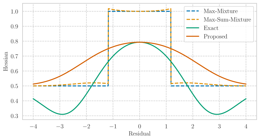
Figure 1: A comparison of the Hessian approximation for a Gaussian mixture factor consisting of two components, both centered around zero but with different covariances. For a scalar cost and state variable, the Hessian is also scalar. When substituted into a local optimization method, a better Hessian approximation results in better convergence. In particular, the proposed Hessian (orange) is much closer visually to the exact Hessian (green) than the Max-Mixture (blue) and Max-Sum-Mixture (yellow) approaches.

Common iterative methods for solving NLS problems, such as Gauss-Newton, rely on an approximation of the Hessian of the cost function. When the Sum-Mixture approach is used in conjunction with such optimization techniques, the resulting Hessian approximation is inaccurate, leading to degraded performance. This inaccuracy was pointed out in [11], but not explained theoretically. The paper [11] then proposes an alternative to the Sum-Mixture approach, termed the Max-Sum-Mixture approach, which is a hybrid between the Max-Mixture and Sum-Mixture approaches. The dominant component of the mixture is factored out, creating a Max-Mixture error term, while the remaining non-dominant factor is treated using the approach of [10]. The Hessian contribution for the non-dominant factor is inaccurate in a similar fashion as that of the Sum-Mixture, and improving on this aspect is the focus of this paper.

The contribution of this paper is a novel Hessian approximation for NLS problems involving GMM terms, which is derived by using the Gauss-Newton Hessian approximation for the component errors corresponding to each component of the GMM, and using the chain rule to take into account the additional nonlinearities. This approach is similar in spirit to how the robust loss nonlinearity is treated in deriving the Triggs correction proposed in [12] and used in the ceres library [13]. Traditional NLS solvers do not allow the user to specify a separate Hessian, only requiring an error definition and its corresponding Jacobian. Therefore, this paper also proposes a method of defining an error and Jacobian that uses the proposed Hessian while maintaining compatibility with the NLS solver.

The more accurate Hessian approximation is showcased in Figure 1 for a simple 1D example, and the improvement in the Hessian accuracy leads to improved convergence properties of gradient-based optimization methods. The benefits of the proposed approach are demonstrated on a toy problem, a simulated point-set registration problem [11], [14] and on a SLAM problem with unknown data associations on the “Lost in the Woods” dataset [15]. The implementation is open-sourced at https://github.com/decargroup/hessian_sum_mixtures and uses a modified version of the navlie NLS solver [16].

The rest of this paper is organized as follows. Newton’s method and the Gauss-Newton Hessian approximation for NLS are presented in Sec. II. Sec. III presents Gaussian mixtures, the difficulties in applying NLS to Gaussian mixtures, as well as a review of the previous approaches to solving this problem. Sec. IV discusses the reasons for the Hessian inaccuracy of existing methods, and Sec. V presents the proposed approach. Sec. VI describes how to maintain compability with traditional NLS solvers while using the proposed Hessian. Sec. VII presents simulation and experimental results highlighting the benefits of the proposed approach.

II Theoretical Background

Popular optimization methods used for state estimation are reviewed to motivate the improvement of the Hessian approximation used. Furthermore, the link to NLL minimization of Gaussian probabilities is reviewed, while Sec. III presents the extension to GMMs.

II-A Newton’s Method

Newton’s method is a local optimization method that iteratively minimizes a quadratic approximation to the loss function [1, §4.3.1]. Denoting the optimization variable as $\mbf{x}\in\mathbb{R}^{n}$ and the loss function to be minimized as $J(\mbf{x})$, Newton’s method begins with an initial guess $\mbf{x}^{(0)}$, and iteratively updates the optimization variable using

$$\mbf{x}^{(i+1)} =\mbf{x}^{(i)}+\alpha^{(i)}\Delta\mbf{x}^{(i)},$$ (1)

where $\alpha^{(i)}$ is a user-defined step size and $\Delta\mbf{x}^{(i)}$ is the descent direction. Setting the gradient of the local quadratic approximation of the loss at $\mbf{x}^{(i)}$ to zero results in the descent direction being given by [17, §2.2]

$$\frac{\partial^{2}J(\mbf{x})}{\partial\mbf{x}\partial\mbf{x}^{\mathsf{T}}}\Delta\mbf{x} =-\frac{\partial J(\mbf{x})}{\partial\mbf{x}^{\mathsf{T}}},$$ (2)

where $\frac{\partial J(\mbf{x})}{\partial\mbf{x}}$ and $\frac{\partial^{2}J(\mbf{x})}{\partial\mbf{x}\partial\mbf{x}^{\mathsf{T}}}$ are the Jacobian and Hessian respectively, and are evaluated at the current iterate $\mbf{x}^{(i)}$. The notation $\frac{\partial J(\mbf{x})}{\partial\mbf{x}^{\mathsf{T}}}=\left(\frac{\partial J(\mbf{x})}{\partial\mbf{x}}\right)^{\mathsf{T}}$ is used throughout this paper. The iterate $\mbf{x}^{(i)}$ is updated using (1) and the process is iterated to convergence. The main drawbacks of this method are the need to compute the Hessian, as well as the requirement for the Hessian to be positive definite. The Hessian is only guaranteed to be positive semidefinite for convex losses [18, §3.1.4], which are infrequent in robotics applications.

II-B Gauss-Newton Method

The Gauss-Newton method is an optimization approach applicable to problems that have a NLS structure. The loss function is written as the sum of squared error terms,

$$J(\mbf{x}) =\sum_{i=1}^{{n_{f}}}J_{i}(\mbf{x})=\sum_{i=1}^{{n_{f}}}\frac{1}{2}\mbf{e}_{i}(\mbf{x})^{\mathsf{T}}\mbf{e}_{i}(\mbf{x}),$$ (3)

where $J_{i}(\mbf{x})$ denotes a single summand, and ${n_{f}}$ is the number of summands. The Jacobian and Hessian are computed using the chain rule,

$$\frac{\partial J(\mbf{x})}{\partial\mbf{x}} =\sum_{i=1}^{{n_{f}}}\frac{\partial J(\mbf{x})}{\partial\mbf{e}_{i}}\frac{\partial\mbf{e}_{i}}{\partial\mbf{x}},$$ (4)

$$\frac{\partial^{2}J(\mbf{x})}{\partial\mbf{x}\partial\mbf{x}^{\mathsf{T}}} =\sum_{i=1}^{{n_{f}}}\left(\frac{\partial\mbf{e}_{i}}{\partial\mbf{x}}^{\mathsf{T}}\frac{\partial\mbf{e}_{i}}{\partial\mbf{x}}+\sum_{j=1}^{{n_{\textrm{e}}}_{i}}e_{i,j}\frac{\partial^{2}e_{i,j}}{\partial\mbf{x}\partial\mbf{x}^{\mathsf{T}}}\right),$$ (5)

where the argument $\mbf{x}$ has been dropped in writing $\mbf{e}_{i}$. The Gauss-Newton approximation sets the second term of (5) to zero, such that

$$\frac{\partial^{2}J(\mbf{x})}{\partial\mbf{x}\partial\mbf{x}^{\mathsf{T}}} \approx\mbf{H}_{\text{GN}}=\sum_{i=1}^{{n_{f}}}\frac{\partial\mbf{e}_{i}}{\partial\mbf{x}}^{\mathsf{T}}\frac{\partial\mbf{e}_{i}}{\partial\mbf{x}},$$ (6)

where $\mbf{H}_{\text{GN}}$ is the Hessian approximation made by Gauss-Newton. For an error term $\mbf{e}_{i}(\mbf{x})$ affine in $\mbf{x}$, this approximation is exact, and the algorithm converges in a single iteration.

II-C Maximum a Posteriori Estimation

Maximum a Posteriori (MAP) estimation seeks to estimate the system state $\mbf{x}\in\mathbb{R}^{n}$ by maximizing the posterior probability [1, Sec. 3.1.2], which for Gaussian error models results in the optimization problem

$$\hat{\mbf{x}} =\operatorname*{arg\,min}_{\mbf{x}}\sum_{i=1}^{{n_{f}}}-\log\mathcal{N}\left(\boldsymbol{\eta}_{i}(\mbf{x});\boldsymbol{\mu}_{i},\mbf{R}_{i}\right),$$ (7)

where $\mathcal{N}\left(\boldsymbol{\eta}_{i};\boldsymbol{\mu}_{i},\mbf{R}_{i}\right)$ is a Gaussian probability density function (PDF) in the error $\boldsymbol{\eta}_{i}$ with mean $\boldsymbol{\mu}_{i}$ and covariance $\mbf{R}_{i}$. The MAP estimation problem results in an NLS problem of the form (3), with the the normalized error $\mbf{e}_{i}(\mbf{x})$ obtained through the change of variables

$$\mbf{e}_{i}(\mbf{x}) =\sqrt{\mbf{R}_{i}^{-1}}(\boldsymbol{\eta}_{i}(\mbf{x})-\boldsymbol{\mu}_{i}).$$ (8)

For non-Gaussian error models, the Gaussian in (7) is replaced by an arbitrary PDF $p(\boldsymbol{\eta}_{i})$ resulting in a more general summand expression $J_{i}(\mbf{x})=-\log p(\boldsymbol{\eta}_{i})+c_{i}$ in (3). The constant $c_{i}$ absorbs extraneous normalization constants from $-\log p(\boldsymbol{\eta}_{i})$ that do not affect the optimization.

III Gaussian Mixture Error Terms

A possible choice for the error model probability $p_{i}\left(\cdot\right)$ is a Gaussian mixture model. Gaussian mixture models are the sum of $n_{k}$ weighted Gaussian components, allowing for a wide range of arbitrary probability distributions to be easily represented. The expression for a single Gaussian mixture term, with the term index $i$ omitted for readability, is given by

$$p(\mbf{x}) =\sum_{{k}=1}^{{n_{k}}}w_{k}\mathcal{N}\left(\boldsymbol{\eta}_{k}(\mbf{x});\boldsymbol{\mu}_{k},\mbf{R}_{k}\right),$$ (9)

where $w_{k}$ is the weight of the $k$’th Gaussian component. Note that here the sum is over components, whereas in Sec. II the sums considered are over problem error terms, of which only a single one is now considered. To find an expression of the NLL for error models of the form (9), first let $\alpha_{k}$ be the weight normalized by covariance, written as

$$\alpha_{k} =w_{k}\det(\mbf{R}_{k})^{-1/2}.$$ (10)

Then, dropping state- and covariance-independent normalization constants and using the change of variables (8) yields the expression for the corresponding summand given by

$$J_{\text{GMM}}(\mbf{x}) =-\log p(\mbf{x})+c$$ (11)

$$=-\log\sum_{{k}=1}^{{n_{k}}}\alpha_{k}\exp\left(-\frac{1}{2}\mbf{e}_{k}(\mbf{x})^{\mathsf{T}}\mbf{e}_{k}(\mbf{x})\right).$$ (12)

The summand corresponding to a Gaussian mixture model NLL, given by (12), is not of the form of a standard NLS problem in (3). Unlike with Gaussian error terms, an NLS problem cannot be directly obtained, since the logarithm does not cancel the exponent. Hence, standard NLS optimization methods, such as Gauss-Newton, are not directly applicable to problems with Gaussian mixture error terms. Three existing approaches have been proposed to utilize Gaussian mixture terms within the framework of NLS, as discussed in the following sections.

III-A Max-Mixtures

The Max-Mixture approach, first introduced in [9], replaces the summation in (12) with a $\max$ operator, such that the NLL is given by

$$-\log p_{\max}(\mbf{x}) =-\log\left(\max_{k}\alpha_{k}\exp\left(-\frac{1}{2}\mbf{e}_{k}(\mbf{x})^{\mathsf{T}}\mbf{e}_{k}(\mbf{x})\right)\right).$$

The key is that the $\max$ operator and the logarithm may be swapped, allowing the logarithm to be pushed inside the $\max$ operator to yield the Max-Mixture error, given by

$$-\log p_{\max}(\mbf{x}) =-\log\alpha_{k}+\frac{1}{2}\mbf{e}_{{k}^{*}}(\mbf{x})^{\mathsf{T}}\mbf{e}_{{k}^{*}}(\mbf{x}),$$ (13)

where

$${{k}^{*}}=\operatorname*{arg\,max}_{{k}}\alpha_{k}\exp\left(-\frac{1}{2}\mbf{e}_{k}(\mbf{x})^{\mathsf{T}}\mbf{e}_{k}(\mbf{x})\right)$$ (14)

is the integer index of the dominant mixture component at any given $\mbf{x}$. The Max-Mixture error in (13) is in the standard NLS form, and methods such as Gauss-Newton can be used to solve the problem.

III-B Sum-Mixtures

A general method for treating non-Gaussian likelihoods in NLS is proposed in [10]. For a general non-Gaussian NLL $-\log p_{\textrm{non-gauss}}(\mbf{x})$, the corresponding NLS error $e_{\textrm{non-gauss}}(\mbf{x})$ is derived by writing the relationship

$$J_{\textrm{SM}}(\mbf{x}) =-\log p_{\textrm{non-gauss}}(\mbf{x})+c$$ (15)

$$=\frac{1}{2}\left(\sqrt{\log{\gamma_{\text{{{SM}}}}}-\log p_{\textrm{non-gauss}}(\mbf{x})}\right)^{2},$$ (16)

where ${\gamma_{\text{{{SM}}}}}$ is a normalization constant chosen such that ${\gamma_{\text{{{SM}}}}}\geq\log p_{\textrm{non-gauss}}(\mbf{x})$ to ensure that the square root argument is always positive. In this case, the constant $c$ absorbs the constant offset that is added by the normalization constant. The expression (16) allows the error definition

$$e_{\textrm{non-gauss}}(\mbf{x}) =\sqrt{\log{\gamma_{\text{{{SM}}}}}-\log p_{\textrm{non-gauss}}(\mbf{x})}.$$ (17)

The Sum-Mixture approach consists of applying this approach to the Gaussian mixture case,

$$J_{\text{SM}}(\mbf{x}) =\frac{1}{2}e_{\textrm{SM}}^{2}(\mbf{x})$$ (18)

$$=\frac{1}{2}\left(\sqrt{2}\sqrt{-\log\frac{1}{{\gamma_{\text{{{SM}}}}}}\sum_{{k}=1}^{{n_{k}}}\alpha_{k}\exp\left(-\frac{1}{2}\mbf{e}_{k}^{\mathsf{T}}\mbf{e}_{k}\right)}\right)^{2}.$$ (19)

Ensuring positivity of the square root argument can be achieved by setting the normalization constant to ${\gamma_{\text{{{SM}}}}}=\sum_{k=1}^{n_{k}}\alpha_{k}$ [19].

III-C Max-Sum-Mixtures

The Max-Sum-Mixture is introduced in [11], and is a hybrid between the Max-Mixture and Sum-Mixture approaches. The dominant component of the mixture is factored out such that the corresponding summand is given by

$$J_{\text{MSM}}(\mbf{x}) =\frac{1}{2}\mbf{e}_{{{k}^{*}}}^{\mathsf{T}}\mbf{e}_{{k}^{*}}$$ (20)

$$\quad-\log\sum_{k=1}^{n_{k}}\alpha_{k}\exp\left(-\frac{1}{2}\mbf{e}_{k}^{\mathsf{T}}\mbf{e}_{k}+\frac{1}{2}\mbf{e}_{{{k}^{*}}}^{\mathsf{T}}\mbf{e}_{{k}^{*}}\right).$$

The first term of (III-C) is analogous to the Max-Mixture case. The second term is treated using the Sum-Mixture approach,

$$e_{2}(\mbf{x}) =\sqrt{2}\sqrt{-\log\frac{1}{{\gamma_{\text{{{MSM}}}}}}\sum_{k=1}^{n_{k}}\frac{\alpha_{k}}{\alpha_{{k}^{*}}}\exp(-\mbf{e}_{k}^{\mathsf{T}}\mbf{e}_{k}+\mbf{e}_{{{k}^{*}}}^{\mathsf{T}}\mbf{e}_{{k}^{*}})},$$

where ${{\gamma_{\text{{{MSM}}}}}}$ is chosen as ${{\gamma_{\text{{{MSM}}}}}}={n_{k}}\max\frac{\alpha_{k}}{\alpha_{{k}^{*}}}+\delta$. The parameter $\delta>0$ is a damping constant [19] that dampens the influence of this nonlinear term in the optimization.

IV Inaccuracy of the Non-Dominant Component Max-Sum-Mixture Hessian

NLS problems are defined by the choice of error. Different choices of error may be made, which in turn defines the Gauss-Newton Hessian approximation. Because of the Gaussian noise assumption in most robotics problems, the error choice is natural because the negative log-likelihood is quadratic. However, since GMMs do not yield a quadratic log-likelihood, there is no natural error choice. The Sum-Mixture is one such error choice but yields an inaccurate Hessian approximation. The inaccuracy is made clear by considering a problem with a single Gaussian mixture error term of the form (9), having a single mode. The cost function is given by

$$J(\mbf{x})=\frac{1}{2}\mbf{e}(\mbf{x})^{\mathsf{T}}\mbf{e}(\mbf{x}),$$ (21)

and when the Sum-Mixture formulation is applied to this problem, the cost function becomes

$$J(\mbf{x}) =\frac{1}{2}e_{{\textrm{SM}}}(\mbf{x})^{2},$$ (22)

with $e_{{\textrm{SM}}}(\mbf{x})=\sqrt{\mbf{e}^{\mathsf{T}}(\mbf{x})\mbf{e}(\mbf{x})}$. Even for a Gaussian likelihood problem that is easily solved by Gauss-Newton in its original formulation, since the error $e_{{\textrm{SM}}}(\mbf{x})$ is a scalar, the Sum-Mixture approach results in a rank one Gauss-Newton Hessian approximation for the corresponding summand. While this is not an issue within the original application in [10], the Hessian approximation when applied to mixtures is inaccurate.

The fundamental reason for this inaccuracy is that higher-level terms in the NLS Hessian (5) are neglected. Due to the added nonlinearity $e_{{\textrm{SM}}}(\mbf{x})=\sqrt{\mbf{e}^{\mathsf{T}}(\mbf{x})\mbf{e}(\mbf{x})}$, terms get absorbed from the left term of (5) into the right one and end up neglected. Even for well-behaved component errors, the additional nonlinearity imposed by the LogSumExp expression inside the square root in (19), together with the square root itself, make it such that the Gauss-Newton approximation is inaccurate, as demonstrated by the unimodal single-factor case. The Max-Sum-Mixture approach mostly addresses the shortcomings of the Sum-Mixture method by extracting the dominant component.

However, the non-dominant components in the second term of (III-C) are still subjected to the same treatment. Their contribution to the overall Hessian is thus inaccurate, leading to the discrepancies shown in Figure 1. In turn, the inaccurate Hessian negatively affects convergence, since it is used to compute the iteration step (2). Furthermore, it can affect consistency, since the Laplace approximation [7, Sec. 4.4] uses the Hessian to provide a covariance on the resulting state estimate.

V Proposed Approach: Hessian-Sum-Mixture

The proposed approach is termed the “Hessian-Sum-Mixture” (HSM) method and improves on previous formulations by proposing a Hessian that takes into account the nonlinearity of the LogSumExp expression in the GMM NLL (12), while keeping the Gauss-Newton approximation for each component. The overall loss function is exactly the same, up to a constant offset, as for the Sum-Mixture and Max-Sum-Mixture approaches. However, the proposed Hessian derivation does not depend on defining a Gauss-Newton error.

Rather, the proposed Hessian-Sum-Mixture Hessian approximation is derived by setting the second derivatives of the component errors to zero, and using the chain rule to take into account the LogSumExp nonlinearity and derive the cost Hessian.

Formally, by writing the negative LogSumExp nonlinearity as

$$\rho(f_{1},\dots,f_{n_{k}}) =-\log\sum_{{k}=1}^{{n_{k}}}\alpha_{k}\exp(-f_{k}),$$ (23)

and setting the $f_{k}$ components to the quadratic forms $f_{k}\left(\mbf{x}\right)=\frac{1}{2}\mbf{e}_{k}\left(\mbf{x}\right)^{\mathsf{T}}\mbf{e}_{k}\left(\mbf{x}\right)$, the negative Gaussian mixture log-likelihood may be rewritten as $-\log p(\mbf{x})=J(\mbf{x})+c$ with

$$J(\mbf{x}) =\rho(f_{1}(\mbf{e}_{1}(\mbf{x})),\dots,f_{k}(\mbf{e}_{k}(\mbf{x})),\dots f_{n_{k}}(\mbf{e}_{n_{k}}(\mbf{x}))).$$ (24)

Using the Gauss-Newton Hessian approximation for the mixture components yields

$$\frac{\partial^{2}f_{k}(\mbf{x})}{\partial\mbf{x}\partial\mbf{x}^{\mathsf{T}}}\approx\frac{\partial\mbf{e}_{k}}{\partial\mbf{x}^{\mathsf{T}}}\frac{\partial\mbf{e}_{k}}{\partial\mbf{x}}.$$ (25)

Applying the chain rule to (24) and using the approximation (25) yields the factor Jacobian as

$$\frac{\partial J(\mbf{x})}{\partial\mbf{x}} =\sum_{k=1}^{n_{k}}\frac{\partial\rho}{\partial f_{k}}\frac{\partial f_{k}}{\partial\mbf{x}},$$ (26)

and the Hessian as

$$\frac{\partial^{2}J(\mbf{x})}{\partial\mbf{x}\partial\mbf{x}^{\mathsf{T}}} =\sum_{k=1}^{n_{k}}\left(\frac{\partial\rho}{\partial f_{k}}\frac{\partial^{2}f_{k}}{\partial\mbf{x}\partial\mbf{x}^{\mathsf{T}}}+\frac{\partial f_{k}}{\partial\mbf{x}^{\mathsf{T}}}\sum_{j=1}^{n_{k}}\frac{\partial^{2}\rho}{\partial f_{j}f_{k}}\frac{\partial f_{j}}{\partial\mbf{x}}\right).$$ (27)

The partial derivatives of $\rho$ are given by

$$\frac{\partial\rho}{\partial f_{k}} =\frac{\alpha_{k}\exp(-f_{k})}{\sum_{i=1}^{n_{k}}\alpha_{i}\exp(-f_{i})}$$ (28)

$$\frac{\partial^{2}\rho}{\partial f_{j}\partial f_{k}} =\frac{-\delta_{jk}(\alpha_{k}\exp(-f_{k}))\sum_{i=1}^{n_{k}}\alpha_{i}\exp(-f_{i})}{(\sum_{i=1}^{n_{k}}\alpha_{i}\exp(-f_{i}))^{2}}$$

$$\quad+\frac{\alpha_{k}\alpha_{j}\exp(-f_{k})\exp(-f_{j})}{(\sum_{i=1}^{n_{k}}\alpha_{i}\exp(-f_{i}))^{2}},$$ (29)

where $\delta_{jk}$ is the Kronecker delta and the Jacobian of $f_{k}\left(\mbf{x}\right)=\frac{1}{2}\mbf{e}_{k}{\left(\mbf{x}\right)}^{\mathsf{T}}\mbf{e}_{k}{\left(\mbf{x}\right)}$ is given by

$$\frac{\partial f_{k}\left(\mbf{x}\right)}{\partial\mbf{x}} =\mbf{e}_{k}{\left(\mbf{x}\right)}^{\mathsf{T}}\frac{\partial\mbf{e}_{k}{\left(\mbf{x}\right)}}{\partial\mbf{x}}.$$ (30)

Using only the first of the terms in the summand of (27) guarantees a positive definite Hessian approximation since $\frac{\partial\rho}{\partial f_{k}}$ is guaranteed to be positive. The second term has no such guarantee. The final proposed Hessian approximation is

$$\frac{\partial^{2}J\left(\mbf{x}\right)}{\partial\mbf{x}\partial\mbf{x}^{\mathsf{T}}} \approx\mbf{H}_{\text{HSM}}=\sum_{k=1}^{n_{k}}\frac{\partial\rho}{\partial f_{k}}\frac{\partial^{2}f_{k}}{\partial\mbf{x}\partial\mbf{x}^{\mathsf{T}}},$$ (31)

where $\frac{\partial^{2}f_{k}}{\partial\mbf{x}\partial\mbf{x}^{\mathsf{T}}}$ is approximated using (25). Examining (28) allows a somewhat intuitive interpretation of (31). The $\frac{\partial\rho}{\partial f_{k}}$ term is the relative strength of each component at the evaluation point, while $\frac{\partial^{2}f_{k}}{\partial\mbf{x}\partial\mbf{x}^{\mathsf{T}}}$ is the Hessian of that component. The Hessian approximation $\mbf{H}_{\text{HSM}}$ in (31) corresponding to each summand is substituted directly into Newton’s method equation (2), instead of the Gauss-Newton approximation in (6).

The key difference with respect to Max-Sum-Mixture is that the dominant and non-dominant components are all treated in the same manner. In the Max-Sum-Mixture the dominant component has a full-rank Hessian contribution, while the non-dominant components have a rank one Hessian contribution that is inaccurate as detailed in Sec. IV. In situations where the components overlap significantly, the Hessian is thus more accurate in the proposed method.

VI Nonlinear Least Squares Compatibility

Most NLS solvers do not support a separate Hessian definition such that the user may only specify an error and error Jacobian, which then are input to the GN approximation (6). This may be circumvented by engineering an “error” and “error Jacobian” that result in the same descent direction as using Newton’s method (2) with the HSM Hessian (31), while maintaining a similar cost function value to the Sum-Mixture (16). First, defining the following quantities

$$\mbf{e}_{\textrm{solver},1}^{\mathsf{T}} =\begin{bmatrix}\sqrt{\frac{\partial\rho}{\partial f_{1}}}\mbf{e}_{1}^{\mathsf{T}}&\dots&\sqrt{\frac{\partial\rho}{\partial f_{K}}}\mbf{e}_{K}^{\mathsf{T}}\end{bmatrix},$$ (32)

$$\mbf{J}_{\textrm{solver},1}^{\mathsf{T}} =\begin{bmatrix}\sqrt{\frac{\partial\rho}{\partial f_{1}}}\frac{\partial\mbf{e}_{1}}{\partial\mbf{x}^{\mathsf{T}}}&\dots&\sqrt{\frac{\partial\rho}{\partial f_{K}}}\frac{\partial\mbf{e}_{K}}{\partial\mbf{x}^{\mathsf{T}}}\end{bmatrix},$$ (33)

and substituting into the GN Hessian approximation (6) results in exactly the Hessian-Sum-Mixture Hessian (27) as well as the loss Jacobian (26). However, the resulting cost function $\left\|\mbf{e}_{\textrm{solver},1}\right\|_{2}^{2}$ is not of the same form as (12), which can cause issues with methods that use the cost function to guide the optimization such as Levenberg-Marquardt (LM) [17]. To rectify this, an additional error term is required to make the loss into the same form as (12). The proposed error and Jacobian to be input into the solver are thus

$$\mbf{e}_{\textrm{solver}}^{\mathsf{T}} =\begin{bmatrix}\mbf{e}_{\textrm{solver},1}^{\mathsf{T}}&\sqrt{{\gamma_{\text{{{HSM}}}}}+\Delta J}\end{bmatrix},$$ (34)

$$\mbf{J}_{\textrm{solver}}^{\mathsf{T}} =\begin{bmatrix}\mbf{J}_{\textrm{solver, 1}}^{\mathsf{T}}&\mbf{0}\end{bmatrix},$$ (35)

where $\Delta J$ is the difference between the desired loss $J_{\textrm{GMM}}$ (12) and the norm of $\mbf{e}_{\textrm{solver},1}$,

$$\Delta J=J_{\textrm{GMM}}-\left\|\mbf{e}_{\textrm{solver},1}\right\|_{2}^{2},$$ (36)

and ${\gamma_{\text{{{HSM}}}}}$ is a normalization constant that ensures positivity of the square root in (34). The evaluated norm of $\mbf{e}_{\textrm{solver}}$ is thus

$$\left\|\mbf{e}_{\textrm{solver}}\right\|_{2}^{2} =J_{\textrm{GMM}}+{\gamma_{\text{{{HSM}}}}}.$$ (37)

Finding a lower bound on $\Delta J$ that may be used as the normalization constant is difficult. The proposed solution is to set ${\gamma_{\text{{{HSM}}}}}$ to a small initial value. Each time the error is evaluated, the solver determines if ${\gamma_{\text{{{HSM}}}}}+\Delta J$ is less than zero. If yes, ${\gamma_{\text{{{HSM}}}}}$ is updated as ${\gamma_{\text{{{HSM}}}}}\leftarrow\left|\Delta J\right|+\Delta{\gamma_{\text{{{HSM}}}}}$, where $\Delta{\gamma_{\text{{{HSM}}}}}$ is a small positive value. This amounts to moving the entire cost surface upwards. While heuristic, this approach works well in practice and gives almost indistinguishable convergence from a version of the solver that uses the original loss and specifies the Hessian itself.

VII Simulation and Experiments

To show the benefits of the proposed approach, the performance of the Max-Mixture (MM), Max-Sum-Mixture (MSM), Sum-Mixture (SM), the Hessian Sum-Mixture (HSM), and NLS-Hessian Sum-Mixture (NLS-HSM) are all evaluated on two simulated experiments and one real dataset. The HSM approach uses a modified solver that allows specifying the Hessian, while NLS-HSM uses the NLS compatibility method outlined in Sec. VI. The considered simulation examples are similar to the ones provided in [11], and the real-world experiment is a SLAM problem with unknown data associations. In some of the tested examples, particularly the 2D toy example case, the Sum-Mixture approach fails when using standard Gauss-Newton due to a rank-deficient Hessian. To provide a fair comparison, Levenberg-Marquardt [17] (LM) is used instead of Gauss-Newton. LM adds a multiple of the identity to the approximate Hessian, written as $\mbf{H}^{\text{LM}}=\mbf{H}+\lambda\mbf{I}$, where $\lambda$ is a damping constant for the LM method, $\mbf{H}$ is the original Hessian approximation given by (6) for the Max-Mixture, Sum-Mixture, and Max-Sum-Mixture, and by (31) for the Hessian Sum Mixture approach. This ensures that the Hessian approximation is always full rank. The LM damping constant $\lambda$ is chosen as described in [17].

The metrics used to evaluate the quality of the obtained solution are root-mean-squared error (RMSE), defined as

RMSE $$=\sqrt{\frac{1}{N}\sum_{i=1}^{N}\left\|\hat{\mbf{x}}_{i}\ominus\mbf{x}_{i}\right\|_{2}^{2}},$$ (38)

where $\hat{\mbf{x}}_{i}$ and $\mbf{x}_{i}$ are, respectively, the estimated and ground truth states at timestep $i$. The $\ominus$ operator represents a generalized “subtraction” operator, required as some examples considered involve states defined on Lie groups. Following the definitions in [20], a left perturbation is used for all Lie group operations in this paper. Additionally, for states that involve rotations, the difference between the states is split into a rotational and translational component, yielding a rotational RMSE (deg) and a translational RMSE (m).

Consistency, the ability of the estimator to characterize its error uncertainty, is measured using average normalized estimation error squared (ANEES) [21]. A perfectly consistent estimator has ANEES equal to one. The main drawback of this metric is that it characterizes the posterior state belief as Gaussian, which is never completely true in practice.

Lastly, the average number of iterations is used to characterize how quickly the estimator converges to the solution. A smaller number of iterations indicates better descent directions in (2), which is expected if a better Hessian approximation is used. The solver exits once the step size of the LM algorithm is below $1\times 10^{-8}$ or a cap of 200 iterations is reached.

VII-A Toy Example

TABLE I: Results of the toy example Monte Carlo experiment

	Method	RMSE (m)	Iterations	Succ. Rate [%]
1D	MM	4.12e-01	1.43	25.6
	SM	1.26e-02	26.15	99.3
	MSM	1.27e-02	18.77	99.3
	HSM†	1.30e-02	7.15	99.2
	NLS HSM†	1.30e-02	7.16	99.2
2D	MM	6.64e-01	1.57	31.9
	SM	5.38e-02	28.00	97.6
	MSM	4.71e-02	13.03	97.9
	HSM†	4.81e-02	7.10	97.9
	NLS HSM†	4.81e-02	7.10	97.9

The first simulated example consists of optimizing a problem with a Gaussian mixture model error term of the form

$$J(\mbf{x}) =-\log\sum_{{k}=1}^{{n_{k}}}w_{k}\mathcal{N}\left(\mbf{x};\check{\mbf{x}}_{k},\mbf{R}_{k}\right).$$ (39)

The toy example experiments in this section use four mixture components, such that ${n_{k}}=4$. To quantify the performance of all algorithms considered, Monte-Carlo trials are run, where in each trial, random mixture parameters are generated and run for many different initial conditions. Both 1D and 2D examples are considered, where in the 1D case, the design variable is a scalar, and in the 2D case, $\mbf{x}\in\mathbb{R}^{2}$. In all trials, the first mixture component is chosen with weight $w_{1}\sim\mathcal{U}(0.2,0.8)$, where $\mathcal{U}(a,b)$ denotes the uniform distribution over the interval $[a,b]$. The weights for the other mixture components component are chosen as $w_{k}=(1-w_{1})/({n_{k}}-1)$. The mean for the first mixture component is set to $\check{\mbf{x}}_{1}=\mbf{0}$, while each component of the mean of the other mixture components is chosen as $\check{x}_{2}^{i}\sim\mathcal{U}(-2,2)$. The covariance for the first component is set to $\mbf{R}_{1}=\sigma_{1}^{2}\mbf{1}$, where $\sigma_{1}^{2}\sim\mathcal{U}(0.4,1)$. The second component covariance is set to a multiple of the first component such that $\mbf{R}_{2}=m\mbf{R}_{1}$, where $m\sim\mathcal{U}(4,10)$. For each generated set of mixture parameters, the optimization is run from 100 different initial points, chosen uniformly on a grid on $[-4,4]$ for each axis in the problem dimension. Additionally, 1000 different mixture parameters are generated, resulting in a total of 100, 000 Monte-Carlo trials for both the 1D example and 2D example. The ground truth is determined by sampling on a grid combined with local optimization to find the global optimum. The result is marked as converged if it converges to the ground truth within a given threshold, set to $0.01$ meters for all experiments. The results for both the 1D and 2D Monte-Carlo experiments are shown in Table I. In all tables, the proposed method is denoted by ^†. The posterior in this case is extremely non-Gaussian, thus the ANEES is not reported. All methods achieve similar error values, with Sum-Mixture presenting a small improvement over the other methods. Note however that this is due to its interaction with LM, since for the 2D case particularly, the Gauss-Newton version of Sum-Mixture results in a non-invertible Hessian approximation and the method does not work. Nevertheless, the HSM approach still achieves a lower number of iterations than SM or MSM. The Max-Mixture approach achieves the fewest iterations but has a very low success rate.

VII-B Point-Set Registration

TABLE II: Results of the point-set registration experiment.

	Method	RMSE (deg)	RMSE (m)	ANEES	Iter.
2D	MM	1.57e+00	3.27e-02	3.10e+00	13.77
	SM	1.12e+00	1.97e-02	5.10e-02	56.81
	MSM	1.11e+00	1.92e-02	1.60e+00	26.33
	HSM†	1.11e+00	1.92e-02	1.43e+00	23.45
	NLS HSM†	1.11e+00	1.92e-02	1.43e+00	23.45
3D	MM	1.12e+00	2.93e-02	1.82e+00	14.74
	SM	9.57e-01	2.15e-02	2.76e-02	70.21
	MSM	9.59e-01	2.18e-02	1.35e+00	22.93
	HSM†	9.59e-01	2.18e-02	1.27e+00	21.34
	NLS HSM†	9.59e-01	2.18e-02	1.27e+00	21.34

The point-set registration example follows the structure of the example in [11], which itself builds on the formulation of [14]. Given an uncertain source set of points $\mathcal{M}=\left\{{\mbf{m}}_{i}\right\}_{i=1}^{M}$, as well as an uncertain reference set of points ${\mathcal{T}}=\left\{{\mbf{p}}_{j}\right\}_{j=1}^{F}$ with ${\mbf{m}}_{i},{\mbf{p}}_{j}\in\mathbb{R}^{{N}}$, the point-set registration task seeks to find the rigid-body transformation $\mbf{T}_{{t}{s}}^{\star}\in{SE({N})}$ that best aligns ${\mathcal{M}}$ to ${\mathcal{T}}$, where $N$ is either $2$ or $3$. The problem setup is depicted in Figure 2. The transformation is found by forming point-to-point residuals, $\mbf{e}_{ij}$,

$$\mbf{e}_{ij}(\mbf{p}_{j},\mbf{m}_{i},\mbf{C}_{ts},\mbf{r}_{t}^{st}) =\mbf{p}_{j}-\mbf{C}_{ts}\mbf{m}_{i}-\mbf{r}_{t}^{st},$$ (40)

where $\mbf{C}_{ts}\in SO(N)$ and $\mbf{r}_{t}^{st}\in\mathbb{R}^{N}$ are the rotation and translation components of $\mbf{T}_{ts}$, respectively. These errors are assumed Gaussian $\mbf{e}_{ij}\sim\mathcal{N}\left(\mbf{e}_{ij};\ \mbf{0},\mbf{R}_{ij}\right)$ with covariance

$$\mbf{R}_{ij}=\mbf{C}_{ts}\boldsymbol{\Sigma}_{m}\mbf{C}_{ts}^{\mathsf{T}}+\boldsymbol{\Sigma}_{f},$$ (41)

where $\boldsymbol{\Sigma}_{m}$, $\boldsymbol{\Sigma}_{f}$ are the noise covariances on point measurements of points in ${\mathcal{M}}$ and ${\mathcal{T}}$, respectively. Similarly to [11], to incorporate data association ambiguity, the likelihood of a measurement $\mbf{m}_{i}$ is given by the Gaussian mixture

$$p(\mbf{m}_{i}|\mbf{C}_{ts},\mbf{r}_{t}^{st},{\mathcal{T}}) =\sum_{j=1}^{M}w_{j}\mathcal{N}\left(\mbf{e}_{ij}(\mbf{p}_{j},\mbf{m}_{i},\mbf{C}_{ts},\mbf{r}_{t}^{st});\mbf{0},\mbf{R}_{ij}\right),$$

with uniform weights $w_{j}=\frac{1}{M}$. 100 different landmark configurations are generated, with 100 different noisy point-cloud pairs generated for each. The experiments are run for a planar 2D case where $N=2$, and a 3D case where $N=3$. For the 2D (3D) case, each landmark configuration is simulated by first generating 15 (20) landmarks where each position component is generated according to $\mathcal{U}\sim(-5,5)$, followed by duplicating $30\%$ of them 4 times in a Gaussian with $0.1\mbf{1}$ covariance around the original. 100 measurement pairs are then generated for each landmark. The uncorrupted measurements are generated using the ground truth transformation $\mbf{T}_{{t}{s}}$. The groundtruth transformation itself is randomly sampled as $\mbf{T}_{{t}{s}}=\exp(\boldsymbol{\xi}_{{t}{s}}^{\wedge})$, where $(\cdot)^{\wedge}:\mathbb{R}^{m}\to\mathfrak{g}$, with $m=3$ for $SE(2)$ and $m=6$ for $SE(3)$, and $\exp\left(\cdot\right):\mathfrak{g}\to G$ is the corresponding exponential map for $SE(2)$ or $SE(3)$. The Lie group and its corresponding Lie algebra are denoted $G$ and $\mathfrak{g}$ respectively. In all presented experiments, $\boldsymbol{\xi}_{{t}{s}}^{\mathsf{T}}=\begin{bmatrix}\boldsymbol{\xi}^{\phi^{\mathsf{T}}}&\boldsymbol{\xi}^{\textrm{r}^{\mathsf{T}}}\end{bmatrix}$ with $\boldsymbol{\xi}^{\phi}\sim\mathcal{U}(-\frac{15}{180},\frac{15}{180})$, and $\boldsymbol{\xi}^{\textrm{r}}\sim\mathcal{U}(-0.5,0.5)$. The source and target point covariances $\boldsymbol{\Sigma}_{m},\boldsymbol{\Sigma}_{f}$ are each generated randomly as $\boldsymbol{\Sigma}=\mbf{C}\mbf{D}\mbf{C}^{\mathsf{T}}$, where $\mbf{D}$ is a diagonal matrix with entries generated from $\mathcal{U}(0.1,0.6)$ and $\mbf{C}\in SO(N)$ is a random direction-cosine-matrix generated as $\mbf{C}=\exp(\boldsymbol{\xi}^{\wedge})$. Each entry in $\boldsymbol{\xi}$ is generated as $\xi_{i}\sim\mathcal{U}(-\pi,\pi)$, and the $(\cdot)^{\wedge}$ and $\exp(\cdot)$ operators are overloaded for $SO(N)$. Since the state is now defined on a Lie group, the Jacobian and Hessian of the loss with respect to the state are now replaced with their Lie group counterparts [20],

$$\frac{DJ}{D\mathcal{X}} \triangleq\lim_{\boldsymbol{\tau}\rightarrow\mbf{0}}\frac{J(\mathcal{X}\oplus\boldsymbol{\tau})\ominus J(\mathcal{X})}{\boldsymbol{\tau}},$$ (42)

$$\frac{D^{2}J}{D\mathcal{X}^{2}} \triangleq\lim_{\boldsymbol{\tau}\rightarrow\mbf{0}}\frac{\left.\frac{DJ}{D\mathcal{X}}\right|_{\mathcal{X}\oplus\boldsymbol{\tau}}\ominus\left.\frac{DJ}{D\mathcal{X}}\right|_{\mathcal{X}}}{\boldsymbol{\tau}},$$ (43)

where $\oplus$ is the generalized “addition” operator for Lie groups defined analagously to the $\ominus$ operator [20]. The results are presented in Table II. In this case, the proposed HSM approach slightly improves ANEES, as well as improving the number of iterations to convergence. The RMSE is similar for all approaches, with the exception of Max-Mixture, which has a higher RMSE, although it converges the fastest.

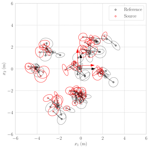
Figure 2: 2D Point-Set Registration Setup. Using the uncertain point positions and measurements, the optimization seeks the transformation from the source frame to the reference frame.

VII-C Lost in the Woods Dataset

TABLE III: Average RMSE (m) on the Lost in the Woods subsequences.

Max Radius (m)	2			4
Subseq. Len (s)	20	30	40	20	30	40
MM	0.30	0.41	0.55	0.14	0.16	0.24
SM	0.44	0.51	0.61	0.40	0.48	0.56
MSM	0.30	0.41	0.54	0.14	0.16	0.24
HSM†	0.30	0.41	0.48	0.14	0.16	0.25
NLS HSM†	0.30	0.41	0.48	0.14	0.16	0.25

TABLE IV: Average iterations on the Lost in the Woods subsequences.

Max Radius (m)	2			4
Subseq. Len (s)	20	30	40	20	30	40
MM	18.7	22.3	27.5	16.7	18.4	24.1
SM	200.0	200.0	200.0	200.0	200.0	200.0
MSM	18.7	22.3	27.6	16.7	18.8	24.4
HSM†	18.7	22.3	27.0	16.7	18.4	24.2
NLS HSM†	18.7	22.2	26.9	16.6	18.4	23.9

The “Lost in the Woods” dataset [15] consists of a wheeled robot navigating a forest of plastic tubes, which are treated as landmarks. The robot receives wheel odometry measurements providing forward velocity and angular velocity measurements. The robot is equipped with a laser rangefinder that provides range-bearing measurements to the landmarks. The task is to estimate the robot poses, $\mathcal{T}=\left\{\mathbf{T}_{1}^{\mathrm{rob}},\ldots,\mathbf{T}_{K}^{\mathrm{rob}}\right\}$, with $\mathbf{T}_{i}^{\mathrm{rob}}\in SE(2),i=1,\ldots,K$, and the landmark positions $\mathcal{L}=\left\{\boldsymbol{\ell}_{1},\ldots,\boldsymbol{\ell}_{n_{\ell}}\right\},\boldsymbol{\ell}_{i}\in\mathbb{R}^{2},i=1,\ldots,n_{\ell}$, given the odometry and range-bearing measurements. The process model consists of nonholonomic vehicle kinematics with the wheel odometry forward and angular velocity inputs detailed in [22]. The range-bearing measurements of landmark $j$ observed from pose $k$ are in the form $\mbf{y}_{jk}=\mbf{g}\left(\mbf{T}_{k}^{\mathrm{rob}},\boldsymbol{\ell}_{j}\right)+\mbf{v}_{jk}$, where $\mbf{v}_{jk}\sim\mathcal{N}\left(\mbf{0},\mbf{R}_{jk}\right)$ and $\mbf{g}\left(\cdot,\cdot\right)$ is the range-bearing measurement model, also detailed in [22]. While the dataset provides the data-association variables (i.e., which landmark each measurement corresponds to), to evaluate the performance of the algorithms, the challenging example of unknown data associations is considered. When the data associations are unknown, a multimodal measurement likelihood may be used, as in [4], where each measurement could have been produced from any landmark in $\mathcal{L}$, such that

$$p(\mbf{y}_{k}|\mbf{T}_{k}^{\mathrm{rob}},\mathcal{L}) =\sum_{j=1}^{{n_{\ell}}}w_{i}\mathcal{N}\left(\mbf{y}_{k}-\mbf{g}(\mbf{T}_{k}^{\mathrm{rob}},\boldsymbol{\ell}_{j});\mbf{0},\mbf{R}_{jk}\right).$$ (44)

The optimization problem to be solved then consists of process model residuals corresponding to the nonholonomic vehicle dynamics, as well as multimodal range-bearing error terms of the form (44) for each measurement. To simplify the problem, it is assumed that the groundtruth number of landmarks are known, so that the number of components in each mixture (44) is known a priori. Additionally, it is assumed that an initial guess for each landmark position is available. This is similar to the setup of the “oracle baseline” described in [23]. The dataset provides odometry and landmark measurements at 10 Hz. To reduce the problem size, the landmark measurements are subsampled to 1 Hz.

To provide an initial guess of the robot states and the landmark states, robot poses are initialized through dead-reckoning the wheel odometry measurements, while the landmarks are initialized by inverting the measurement model for the first measurement of each landmark. Note that the initialization of the landmark positions utilizes the data association labels, but the actual optimization solves for the associations implicitly using the multimodal likelihoods for each measurement.

The dataset of length 1200 seconds is split into subsequences of length $T_{\text{subseq}}$ seconds each, such that there is no overlap between subsequences. The performance metrics computed for each subsequence to each subsequence are averaged to provide mean metrics. For each subsequence length, two scenarios are considered that correspond to different limits $r_{\textrm{max}}$ on the range of the range-bearing measurements used.

For each subsequence length and maximum range radius, the average RMSE and the average number of iterations are summarized in Table III and Table IV, respectively. The difficulty of the problem increases with the subsequence length, because the deadreckoned initialization becomes further from the true solution. The difficulty also increases with a smaller maximum measurement radius, since fewer measurements are used. For all methods, the RMSE increases with the scenario difficulty, as expected. The HSM method provides a performance improvement in the $r_{\textrm{max}}=2\ \text{m},T_{\text{subseq}}=40\ \text{s}$ case, which corresponds to the hardest difficulty considered. In the other scenarios, all methods perform similarly. The number of iterations also presents a slight improvement in the same case of $r_{\textrm{max}}=2\ \text{m},T_{\text{subseq}}=40\ \text{s}$, while showing similar performance in the other scenarios.

VIII Conclusion

This paper proposes deriving a Hessian approximation that takes into account the LogSumExp nonlinearity proper to the negative log-likelihood of the Gaussian mixture, resulting in an improved Hessian approximation. Convergence improvements are demonstrated in simulation and experiment. Furthermore, the proposed method has better mathematical properties in the sense that all mixture components contribute in the same way to the Hessian, without treating the dominant component in a different framework than the rest. A method of maintaining compatibility with traditional NLS solvers is proposed.

While improving convergence, the proposed method remains a local optimization method, requiring a good enough initial guess for proper operation. Future work will consider global convergence properties of the solution, as well as address the non-Gaussian nature of the posterior that arises when considering multimodal likelihoods.

References

- [1] Timothy D. Barfoot “State Estimation for Robotics” Cambridge, UK: Cambridge University Press, 2017 DOI: 10.1017/9781316671528
- [2] Mei Yi Cheung et al. “Non-Gaussian SLAM Utilizing Synthetic Aperture Sonar” In IEEE International Conference on Robotics and Automation (ICRA), 2019, pp. 3457–3463
- [3] Paul Newman and John Leonard “Pure Range-Only Sub-Sea SLAM” In IEEE International Conference on Robotics and Automation (ICRA), 2003, pp. 1921–1926
- [4] Kevin J Doherty, David P Baxter, Edward Schneeweiss and John J Leonard “Probabilistic Data Association via Mixture Models for Robust Semantic SLAM” In IEEE International Conference on Robotics and Automation (ICRA), 2020, pp. 1098–1104
- [5] Johannes Pöschmann, Tim Pfeifer and Peter Protzel “Factor Graph Based 3D Multi-Object Tracking in Point Clouds” In IEEE/RSJ International Conference on Intelligent Robots and Systems (IROS), 2020, pp. 10343–10350
- [6] Gim Hee Lee, Friedrich Fraundorfer and Marc Pollefeys “Robust Pose-Graph Loop-Closures with Expectation-Maximization” In IEEE/RSJ International Conference on Intelligent Robots and Systems (IROS), 2013, pp. 556–563
- [7] Christopher M. Bishop “Pattern Recognition and Machine Learning” New York, NY, USA: Springer, 2006
- [8] Ming Hsiao and Michael Kaess “MH-iSAM2: Multi-Hypothesis iSAM Using Bayes Tree and Hypo-Tree” In IEEE International Conference on Robotics and Automation (ICRA), 2019, pp. 1274–1280
- [9] Edwin Olson and Pratik Agarwal “Inference on Networks of Mixtures for Robust Robot Mapping” In The International Journal of Robotics Research 32.7 SAGE Publications Ltd STM, 2013, pp. 826–840 DOI: 10.1177/0278364913479413
- [10] David M. Rosen, Michael Kaess and John J. Leonard “Robust Incremental Online Inference over Sparse Factor Graphs: Beyond the Gaussian Case” In IEEE International Conference on Robotics and Automation (ICRA), 2013, pp. 1025–1032 DOI: 10.1109/ICRA.2013.6630699
- [11] Tim Pfeifer, Sven Lange and Peter Protzel “Advancing Mixture Models for Least Squares Optimization” In IEEE Robotics and Automation Letters (RA-L) 6.2, 2021, pp. 3941–3948 DOI: 10.1109/LRA.2021.3067307
- [12] Bill Triggs, Philip F McLauchlan, Richard I Hartley and Andrew W Fitzgibbon “Bundle Adjustment—a Modern Synthesis” In Vision Algorithms: Theory and Practice, 2000, pp. 298–372 Springer
- [13] Sameer Agarwal, Keir Mierle and The Ceres Solver Team “Ceres Solver”, 2023 URL: https://github.com/ceres-solver/ceres-solver
- [14] Bing Jian and Baba C. Vemuri “Robust Point Set Registration Using Gaussian Mixture Models” In IEEE Transactions on Pattern Analysis and Machine Intelligence 33.8, 2011, pp. 1633–1645 DOI: 10.1109/TPAMI.2010.223
- [15] Timothy D. Barfoot “AER1513 Course Notes, Assignments, and Data Sets” In University of Toronto, Institute for Aerospace Studies, 2011
- [16] Charles Champagne Cossette et al. “navlie: A Python Package for State Estimation on Lie Groups” In IEEE/RSJ International Conference on Intelligent Robots and Systems (IROS), 2023, pp. 5282–5287 IEEE
- [17] Kaj Madsen, Hans Bruun Nielsen and Ole Tingleff “Methods for Nonlinear Least Squares Problems” Technical University of Denmark, 2004
- [18] Stephen P Boyd and Lieven Vandenberghe “Convex Optimization” Cambridge University Press, 2004
- [19] Tim Pfeifer “Adaptive Estimation Using Gaussian Mixtures”, 2023
- [20] Joan Solà, Jeremie Deray and Dinesh Atchuthan “A micro Lie Theory for State Estimation in Robotics”, 2021, pp. 1–17 arXiv: http://arxiv.org/abs/1812.01537
- [21] X Rong Li, Zhanlue Zhao and Vesselin P Jilkov “Estimator’s Credibility and its Measures” In Triennial World Congress, 2002
- [22] Charles Champagne Cossette, Alex Walsh and James Richard Forbes “The Complex-Step Derivative Approximation on Matrix Lie Groups” In IEEE Robotics and Automation Letters (RA-L) 5.2, 2020, pp. 906–913 DOI: 10.1109/LRA.2020.2965882
- [23] Yihao Zhang et al. “Data-Association-Free Landmark-based SLAM” In IEEE International Conference on Robotics and Automation (ICRA), 2023 DOI: 10.1109/ICRA48891.2023.10160719