Action-conditioned video generation with new indoor robot motion dataset RoAM

Abstract

Long-term video generation and prediction remain challenging tasks in computer vision, particularly in partially observable scenarios where cameras are mounted on moving platforms. The interaction between observed image frames and the motion of the recording agent introduces additional complexities. In response, we introduce the Action-Conditioned Video Generation (ACVG) framework, a novel approach that investigates the intricate relationship between actions and generated image frames through a deep dual Generator-Actor architecture. ACVG generates video sequences conditioned on the actions of robots, enabling exploration and analysis of how vision and action mutually influence one another in dynamic environments. We evaluate the framework’s effectiveness on the RoAM dataset, conducting a comprehensive empirical study comparing ACVG to other state-of-the-art frameworks along with a detailed ablation study.

1 Introduction

The significance of prediction in intelligence is widely recognized [bubic]. While self-attention-based transformer models have revolutionized language prediction and generation [Vaswani_attention2017], the same level of advancement has not been achieved in the domain of video and image prediction models. However, long-term reliable video prediction is a valuable tool for decoding essential information about the environment, providing a data-rich format that can be leveraged by other learning frameworks like policy gradient [Kaiser2020] or planning algorithms [Hafner2019]. However, the complex interactions among objects in a scene pose significant challenges for long-term video prediction [finn, finn2, mathieu, villegas, GaoCVPR2020, villegasNeurIPS2019]. Based on the state-of-the-art literature, multi-time step video prediction can be broadly categorized into two types: (i) Video prediction in a fully observable static background, where the camera remains stationary during recording [finn2, mathieu, villegas]; and (ii) Video prediction in a dynamic background, where the camera is mounted on a moving platform, such as a car or a mobile robot. The latter case is often called prediction in a partially observable scenario [GaoCVPR2020], [villegas],[villegasNeurIPS2019],[sarkar2021]. Partial observability arises due to the continuous occlusion of the background caused by the camera’s motion. This is the scenario in which we are interested.

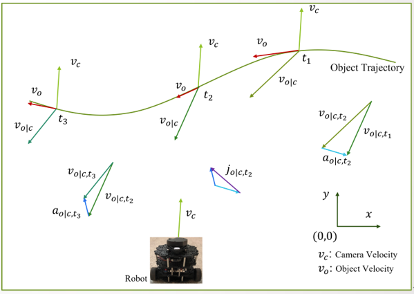
Figure 1: Representation of the interplay between the action taken by the recording robotic agent and the observed relative motion and trajectory of an object in the image frame with vector diagram

Over the past decade, the primary focus in studying the spatio-temporal dynamics of video prediction has largely revolved around fully observable environments with static cameras [srivastava, oh, vondrick, finn, mathieu, villegas, xu, WichersICML2018]. These frameworks often utilize optical flow and content decomposition approaches to generate pixel-level predictions. Adversarial training is commonly employed to enhance the realism of the generated images. However, with the increasing availability of computational power, there is a recent trend towards generating high-fidelity video predictions using various generative architectures, such as Generative Adversarial Networks (GAN) and Variational Autoencoders (VAE) [LiangICCV2017, Denton, BabaeizadehICLR2018, LeeICLR2018, CastrejonICCV2019, GaoCVPR2020, villegasNeurIPS2019].

In the partially observable scenario frequently encountered in autonomous robots and cars, prediction faces significant challenges due to the intricate relationship between the robot’s movements and the visual data captured by its camera. The dynamics of the robot play a crucial role in conditioning each pixel of data recorded by the camera sensor [sarkar2021, acpnet2023]. This is illustrated with the vector diagram in Fig. 1 where $v_{c}$ represents the instantaneous velocity of the recording platform, in this case, a robot and $v_{o}$ is the instantaneous velocity of the object in the environment. However, due to the relative motion between the camera frame and the object the observed velocity of the object with respect to the moving camera frame can be represented as $v_{o|c}$. Similarly, we can further represent the observed acceleration and jerk of the object with respect to the camera frame as $a_{o|c}$ and $j_{o|c}$ respectively. Thus, from figure 1 it is very clear that the action (in this case the velocity ) of the recording agent plays a crucial role in the observed future trajectories of the object in the image frame. The action also decides the predicted background of the future frames. In the literature, different approaches have been adopted by different researchers to address this same problem over the last 5-6 years.

Like every dynamical system the spatio-temporal dynamics embedded in a partially observable video data with moving camera frame can be represented in the simplest format as:

$$\dot{x}_{t}=f(x_{t},a_{t})$$ (1)

where, $x_{t}$ denotes the image state at time $t$. the control action or movement of the camera is represented with $a_{t}$ and $\dot{x}_{t}$ represents the velocity of the image state $x_{t}$. For high dimensional data like video, the relationship between the velocity of pixel data or optical flow and image frame $x_{t}$ is not so straight forward like given in the toy equation 1, however, the fundamental philosophy behind model such systems still remains the same as Eq. 1. For example in the absence of the action data $a_{t}$, Sarkar et. al. [sarkar2021] with their Velocity Acceleration Network (VANet) modeled the interaction between the camera action and the observed image frame with second-order optical flow maps. Villegas et. al. [villegasNeurIPS2019] attributed this interaction as stochastic noise and showed with large enough parametric models with higher computing capabilities, we can make longer accurate predictions with video data. Denton et. al. [Denton] modeled this interaction as a learned stochastic prior and recently Franceschi et. al [slrvp2020] showed that video generation problems can be modeled as stochastic latent dynamic models in their variational architecture. with the success of transformer models in natural language problems, recently there has been a lot of interest in designing efficient visual transformers [ViT2021] for video prediction tasks [video_transformer2022, Gao_2022_CVPR_ViT]. Gao et al. [Gao_2019_ICCV] tried to address the occlusion problem arising from the partial observability in KITTI dataset [kitti] by disentangling motion-specific flow propagation from motion-agnostic generation of pixel data for higher fidelity.

However, none of these work explicitly model or incorporate the action data $a_{t}$ of the recording platform. This can be partly attributed to the fact that none of the existing datasets like KITTI [kitti], KITTI 360 [KITTI-360], A2D2 [A2D2] provides the synchronized action data along with the image frames. A recent study by Sarkar et al. [acpnet2023] introduced the RoAM dataset, which includes synchronized robot action-image data. This dataset provides stereo image frames along with time-synchronized action data from the recording autonomous robot. In their work, Sarkar et al. also proposed the Action Conditioned Prediction Network (ACPNet), which is the first framework to explicitly incorporate the action of the robotic agent as part of the video data modeling process.

While ACPNet [acpnet2023] harnessed control action data to enhance frame prediction accuracy, it did not delve into comprehending the intricate interplay between action $a_{t}$ and $x_{t}$. Predicted image frames indeed rely on the actions taken by the mobile agent, but conversely, future actions by the agent often depend on the current system state, i.e., $a_{t}=g(x_{t})$. Enhanced predictions of the future image state contribute to more accurate approximations of future control actions, and vice versa. This dual dependency highlights the mutual influence between modeling the system controller and the system dynamics derived from video frames. Sarkar et al. [acpnet2023] made an assumption of a constant control action for the entire prediction horizon $T$ instead of modeling the dynamics of the action data $a_{t}$. While this simplification may be acceptable for shorter prediction horizons, for longer durations (larger $T$), the assumption of a constant action can result in inaccuracies in predictions.

We introduce our innovative Action-Conditioned Video Generation (ACVG) framework, designed to capture the dual dependency between the state and action pair through our Generator-Actor Architecture. In addition to a generator architecture that considers the current and past platform actions, our framework features an actor network responsible for predicting the next action, $\tilde{a}_{t+1}$, based on the current observed/predicted image state. Our dual network implicitly encodes the dynamics of the recording platform and its impact on predicted image frames by explicitly modeling and predicting the upcoming course of action through the Actor-Network.

The rest of the paper is organized in the following manner: The mathematical framework of the Generator and Actor network of the proposed ACVG framework is discussed in detail in Section 2 along with loss functions and the training process. Subsequently, we provide concise insights into the partially observable datasets available in Section 3, emphasizing why the RoAM dataset stands out as the ideal choice in the current literature to validate our proposed hypothesis regarding partially observable video data, which is prevalent in the domain of mobile robotics. The experimental setup for training and testing ACVG is given in Section 3. The performance analysis and ablation study of the ACVG compared to four other frameworks: ACVG with fixed action (ACVG-fa), ACPNet, VANet and MCNet with detailed discussions are given in Section 4. Finally, Section 5 concludes the paper with a few remarks regarding the possible future research directions that can be pursued.

2 Action Conditioned Video Generation

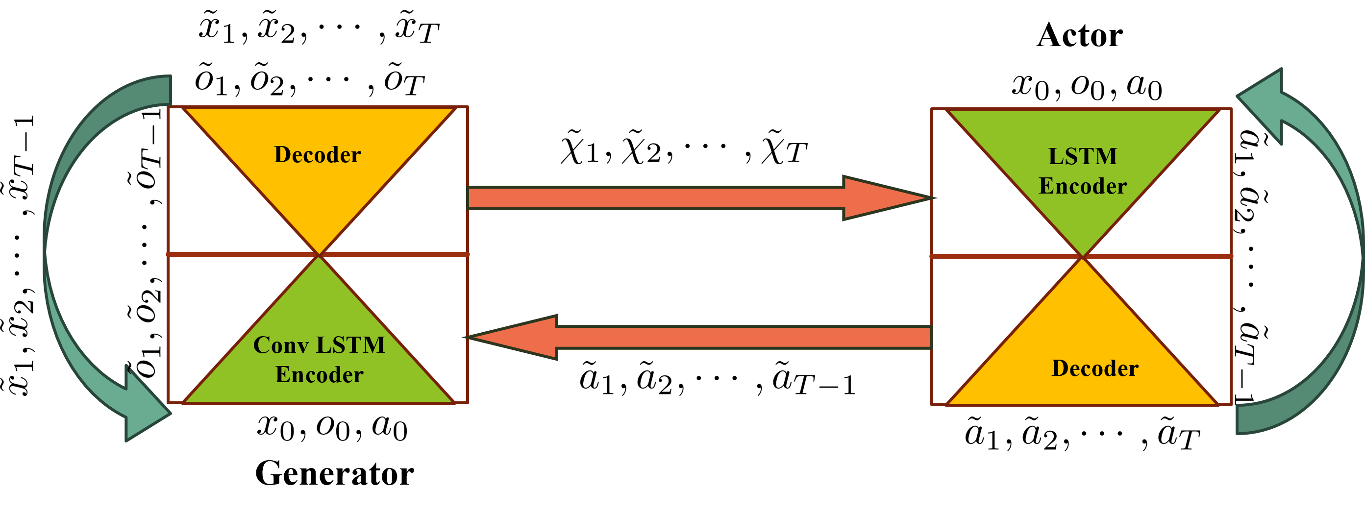
Figure 2: The interdependent training loop of the Generator and Actor network of ACVG.

Let us assume that the current image frame is denoted by $x_{t}\in{\mathbb{R}}^{[\text{image}_{h}\times\text{image}_{w}\times c]}$ where $\text{image}_{h}$, $\text{image}_{w}$ and $c$ denotes the height, width and channel length of the image respectively. in the case of color images like ours $c=3$. We define the first-order pixel flow map or the flow map, $o_{t}\in{\mathbb{R}}^{[\text{image}_{h}\times\text{image}_{w}\times c]}$ at time step $t$ as the following:

$$o_{t}=x_{t}-x_{t-1}$$ (2)

The normalised action at time $t$ is denoted as $a_{t}$ and $a_{t}\in{\mathbb{R}}^{m}$ where $m$ is the dimension of the action space of the mobile agent on which the camera is mounted. We employ normalized actions, $a_{t}$ for the sake of generalization. This normalization approach is particularly useful due to the potential variations in actuator limits among different mobile platforms. Normalizing the action values ensures that our inference framework can scale effectively, accommodating these diverse actuator ranges.

Our objective here is the predict the future image and action state pair $(x_{t},a_{t})$ from $t=1$ till $t=T$ where $T$ is the prediction horizon, give the initial image, flow and action state as $x_{0}$, $o_{0}$ and $a_{t}$ respectively at time $t=0$. For a deterministic dynamical system this would mean an approximation of the following equations:

$$x_{t+1}=x_{t}+{\mathcal{F}}(x_{t},o_{t},a_{t}), \hskip 10.00002pt\text{given, }(x_{0},o_{0},a_{0})$$ (3)

$$a_{t+1}={\mathcal{G}}(x_{t+1},o_{t+1})$$ (4)

where ${\mathcal{F}}$ and ${\mathcal{G}}$ denote the system dynamics and behaviour of the controller respectively which are both unknown to us. In the case of video prediction, the approximation of Eqs. 3 and 4 becomes much more involved and complex due to the high dimensionality of the data and the nature of the complex interactions between the motion of the camera and the motion of the objects as captured in the image plane of the camera.

However, when the high dimensional image information in $x_{t}$ and $o_{t}$ is mapped into a low dimensional feature space as $\hat{x}_{t}$ and $\hat{o}_{t}$ respectively, we can expect to observe similar interaction behaviour between $\hat{x}_{t}$, $\hat{o}_{t}$ and $a_{t}$ similar to Eqs. 3 and 4. However, these interactions might not be in an affine form as suggested in Eq. 3. We approximate these dynamic interactions and predict future image frames with our proposed Action Conditioned Video Generation (ACVG) framework. ACVG is a deep dual network consisting of a Generator and an Actor network. The objective of the generator network is to loosely approximate Eq. 3 whereas the actor network tries to approximate ${\mathcal{G}}$ from Eq. 4.

It’s easily apparent that Equations Eqs. 3 and 4 exhibit a mutual dependence on each other. Similarly, within the Action-Conditioned Video Generation (ACVG) framework, the generator and actor networks share a parallel and interconnected relationship. The dynamics of this relationship are visualized in Figure Fig. 2. In this figure, we can discern that at each time step $t$, the generator network employs the predicted states $\tilde{x}_{t}$ and $\tilde{o}_{t}$, along with the anticipated action state $\tilde{a}_{t}$ generated by the actor network, to forecast the subsequent image frame $\tilde{x}_{t+1}$. This forecasted $\tilde{x}_{t+1}$ is subsequently used by the actor network to project the likely action at time $t+1$, denoted as $\tilde{a}_{t+1}$, which is then fed back into the generator network. This iterative cycle persists until reaching the prediction horizon at time $T$. In this paper $(\tilde{.})$ denotes predicted states.

The initial states, denoted as $x_{0}$ and $o_{0}$, carry a broader interpretation beyond representing the image and flow map solely at time step $t=0$. We employ this overloaded notion of initial state in a more encompassing context, where $x_{0}$ signifies a collection of past observations spanning from $t=-n+1$ to $t=0$ as $x_{0}=\{x_{t=0},x_{t=-1},\cdots,x_{t=(-n+1)}\}$. Likewise, for flow maps, we have $o_{0}=\{o_{t=0},o_{t=-1},\cdots,o_{t=(-n+1)}\}$. It’s worth noting that the computation of flow maps, in accordance with Equation Eq. 2, considers ${o_{(-n+1)}=0}$, as it assumes that at the commencement of our observation at $t=-n+1$, the environment was in a static state. This convention extends to the initial action state as well, and we denote it as $a_{0}=\{a_{t=0},a_{t=-1},\cdots,a_{t=(-n+1)}\}$. In our specific scenario, the minimum number of past observations required is $n_{\min}=2$, as having at least one observed flow map at $t=0$ is essential. However, based on our experimental findings, it is consistently more advantageous to maintain $n\geq 3$ for more robust and improved inference within the generative framework.

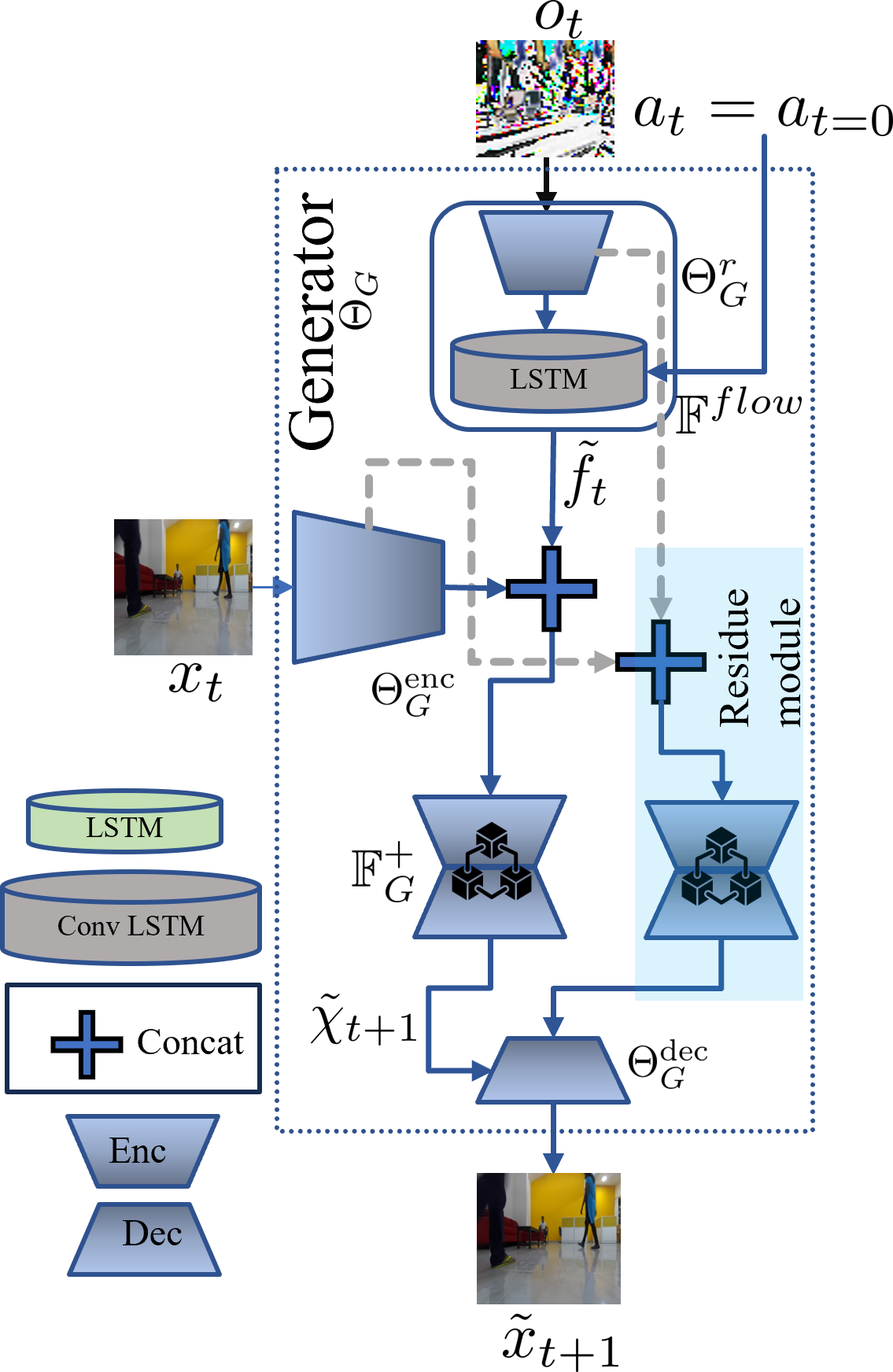
(a)

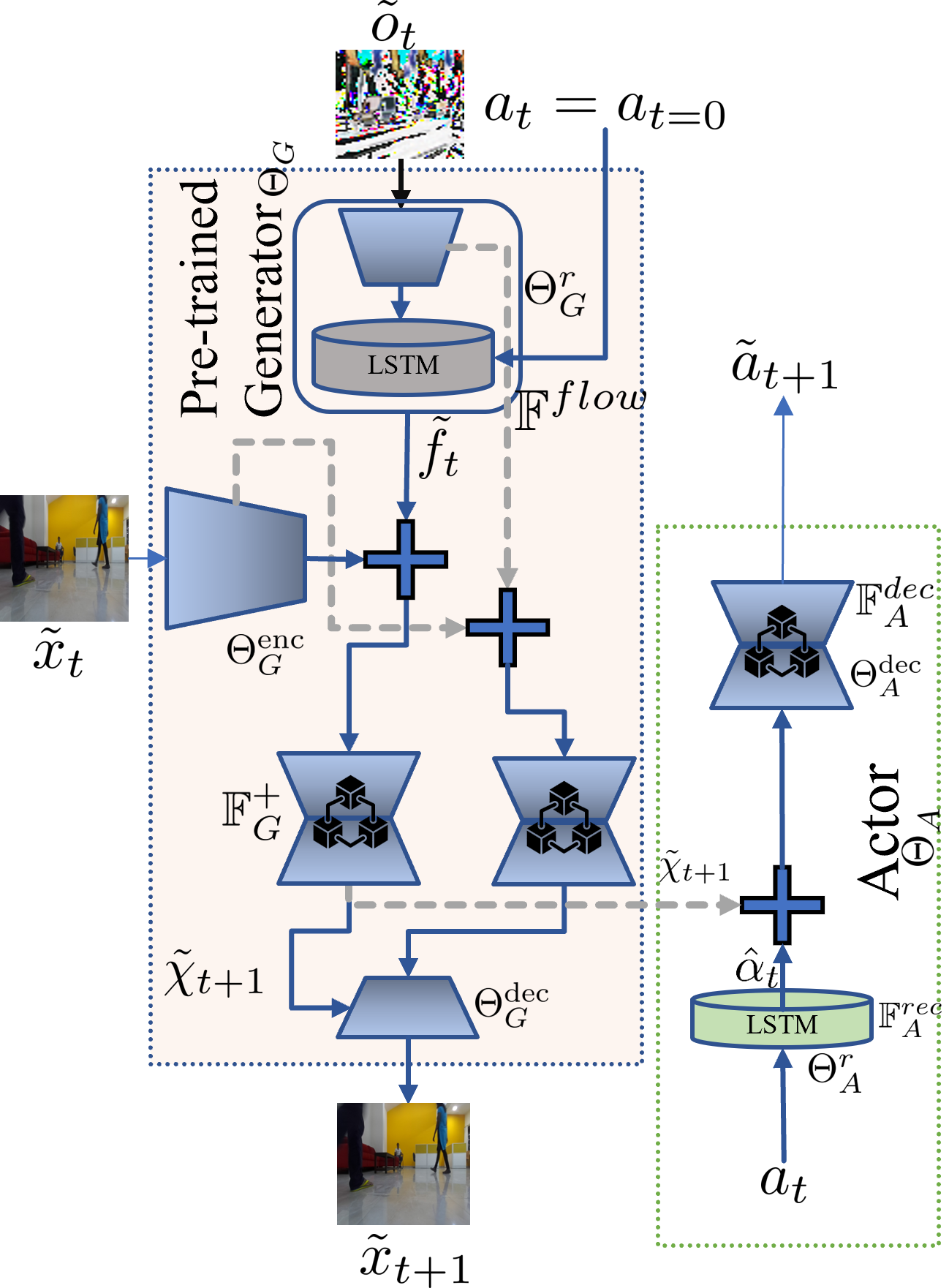
(b)

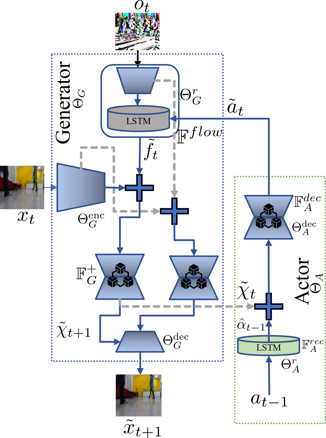
(c)

Figure 3: Architecture of ACVG consists of dual networks: Generator and Actor. Fig. 3(a) shows the architecture of the generator network alone during the generator training phase. During this phase, $\beta=1$ and $\gamma=0$ for the training loss in Eq. 19 and $a_{t}$ is constant. Fig. 3(b) shows the dual configuration of the Generator-Actor framework during the actor training phase. During this phase the weights of the pre-trained generator network is kept frozen. The generator network is used in the inference mode with $\beta=0$ and $\gamma=1$ in Eq. 19. Finally Fig. 3(c) shows the configuration of the network in dual training mode when $\beta=1$ and $\gamma=1$.It’s important to emphasize that in the dual training phase, as depicted in Figure Fig. 3(c), we employ a delayed actor-network to provide the approximate current action $\tilde{a}_{t}$ to the generator network. This delay is necessary because we operate with a causal model, wherein the actor network generates the predicted action $\tilde{a}_{t+1}$ based on the observation of state $\tilde{\chi}_{t+1}$.

2.1 Generator Network

We use stacked recurrent units like Convolutional LSTMs [convlstm] and LSTM cells [lstm] in case of the generator and actor network respectively to iteratively approximate the dynamics from the image and action data. The detailed dual generator-actor network architecture of ACVG is shown in Fig. 3. Our Generator network, is parameterized by $\Theta_{G}$. The parametric space of $\Theta_{G}$ is further divided into 3 groups: $\Theta_{G}=[\Theta^{\text{enc}}_{G},\Theta^{r}_{G},\Theta^{\text{dec}}_{G}]$ where $\Theta^{\text{enc}}_{G}$ denotes the encoder network that maps the image $x_{t}$ and flow maps $o_{t}$ at time $t$ into the low dimensional manifold. This is expressed as :

$$x_{t}\xrightarrow[\Theta^{\text{enc}}_{G}]{Enc}\hat{x}_{t},\hskip 20.00003pto_{t}\xrightarrow[\Theta^{\text{enc}}_{G}]{Enc}\hat{o}_{t}$$ (5)

$\Theta^{r}_{G}$ represent the recurrent part of the network that is designed with stacked convolutional LSTM layers to approximate the spatio-temporal dynamics from the recursive first order flow maps $\hat{o}_{t}$ similar to [villegas],[sarkar2021]. However, unlike the previous works [villegas],[sarkar2021], we use an augmented flow map $\hat{O}_{t}$, where we concatenate the flow map $\hat{o}_{t}$ with the normalised action $a_{t}$ at time $t$ expressed here:

$$\hat{O}_{t}=[\hat{o}_{t},a_{t}]$$ (6)

This augmented flow map, $\hat{O}_{t}$ is then fed to the flow or the recursive module of the generator to approximate the motion kernel $\tilde{f}_{t}$. The flow model ${\mathbb{F}}^{flow}$ approximates the temporal dynamics and interplay between the observed image flow data and the control action taken recording agent $a_{t}$ and is reminiscent of the unknown function ${\mathcal{F}}$ in Eq. 3. However, ${\mathbb{F}}^{flow}$ does it in the parametric space of $\Theta^{r}_{G}$ and on the low dimensional manifold of $\hat{O}_{t}$ expressed here as:

$$\tilde{f}_{t}={\mathbb{F}}^{flow}_{G}(\hat{O}_{t}|\hat{O}_{1:t-1},\Theta^{r}_{G},x_{0},o_{0},a_{0})$$ (7)

Once we have evaluated the motion kernel $\tilde{f}_{t}$ in Eqs. 6 and 7, it is then combined with the current image state in the feature space of $\hat{x}_{t}$ to generate $\tilde{\chi}_{t+1}$:

$$\tilde{\chi}_{t+1}={\mathbb{F}}^{+}_{G}(\hat{x}_{t},\tilde{f}_{t})$$ (8)

The generate $\tilde{\chi}_{t+1}$ is then decoded and mapped back into the original image dimension to generate the predicted image frame $\tilde{x}_{t+1}$ as:

$$\tilde{x}_{t+1}\xleftarrow[\Theta^{\text{dec}}_{G}]{Dec}\tilde{\chi}_{t+1}$$ (9)

where $\Theta^{\text{dec}}_{G}$ denotes the parametric space of the decoder network. If we club the feed-forward components $\Theta^{\text{enc}}_{G}$ and $\Theta^{\text{dec}}_{G}$ together and represent them as ${\mathbb{F}}^{\overline{flow}}_{G}$, then Eqs. 5, 6, 7, 8 and 9 can be represented as :

$$\tilde{x}_{t+1}={\mathbb{F}}^{flow+\overline{flow}}_{G}(\hat{x}_{t},\hat{O}_{t}|\Theta_{G},\hat{O}_{1:t-1},x_{0},o_{0},a_{0})$$ (10)

We can re-arrange and rewrite Eq. 10 as:

$$\tilde{x}_{t+1}={\mathbb{F}}_{G}(x_{t},o_{t},a_{t}|\Theta_{G},x_{0:t-1},o_{0:t-1},a_{0:t-1})$$ (11)

However, during inference generator iteratively uses previously predicted image $(\tilde{x}_{t})$, flow $(\tilde{o}_{t})$ and action $(\tilde{a}_{t})$ states and thus, Eq. 11 can be rewritten as:

$$\tilde{x}_{t+1}={\mathbb{F}}_{G}(\tilde{x}_{t},{\tilde{o}}_{t},\tilde{a}_{t}|\Theta_{G},\tilde{x}_{1:t-1},\tilde{o}_{1:t-1},\tilde{a}_{1:t-1},X_{0})$$ (12)

where $X_{0}=[x_{0},o_{0},a_{0}]$. From the expression for $\tilde{x}_{t+1}$ in the right-hand side (RHS) of Eq. 12, it is very clear that our predicted image frames are conditioned on the predicted control actions $\tilde{a}_{t}$ approximated by the actor network. While Sarkar et. al [acpnet2023] used similar augmentation of action with the image $x_{t}$ for their video generation network, ours ACVG is the first and only framework that explores the augmented flow map $\hat{O}_{t}$ as a means to not only improve the image prediction accuracy but also to capture and predict probable future actions executed by the mobile agent, facilitated by the dual actor network which we discuss next.

2.2 Actor Network

The actor network is parameterized by $\Theta_{A}$, and similar to the generator network, it comprises both a recurrent module and a decoder module. The parametric space $\Theta_{A}$ is further divided into two components: $\Theta_{A}=[\Theta^{r}_{A},\Theta^{\text{dec}}A]$. Here, $\Theta^{r}_{A}$ pertains to the recurrent module of the actor network, while $\Theta^{\text{dec}}A$ encompasses the parameters of the decoder module responsible for generating the predicted action $\tilde{a}_{t+1}$. This predicted action is contingent on the knowledge of the latent image state $\hat{x}_{t+1}$ and the flow map $\hat{o}_{t+1}$. This formulation is parallel to the expression for the control action $a_{t+1}$ in Equation Eq. 4 for dynamical systems.

The recurrent module of the network is built with LSTMcell [lstm] architectures that compute the temporal dynamics encoded in the past action data and can be represented as:

$$\hat{\alpha}_{t}={\mathbb{F}}^{rec}_{A}(a_{t}|\Theta^{r}_{A},a_{0:t-1})$$ (13)

The recurrent module ${\mathbb{F}}^{rec}_{A}$ in Eq. 13 assumes the action $a_{t}$ taken by the robot to be a smooth and continuous function of the image $x_{t}$ and flow state $o_{t}$ and it further assumes that the robot does not make any sudden or jump movements. Thus we use a recurrent architecture to capture these smooth temporal dynamics. With $\hat{\alpha}_{t}$, the predicted action at time step $t+1$ can be generated with latent space information of the future image state $\hat{x}_{t+1}$ and flow map $\hat{o}_{t+1}$ as:

$$\tilde{a}_{t+1}={\mathbb{F}}^{dec}_{G}(\hat{x}_{t+1},\hat{o}_{t+1},\hat{\alpha}_{t}|\Theta^{\text{dec}}_{A})$$ (14)

However, in reality, during inference, we do not have access to the true state information on $\hat{x}_{t+1}$ and $\hat{o}_{t+1}$. Instead, we can have an approximate estimate of the future image flow map $\tilde{\chi}_{t+1}$ generated by the generator network as expressed in Eq. 8. Thus we can estimate Eq. 14 as the following:

$$\tilde{a}_{t+1}={\mathbb{F}}^{dec}_{G}(\tilde{\chi}_{t+1},\hat{\alpha}_{t}|\Theta^{\text{dec}}_{A})$$ (15)

Therefore, by considering Eq. 15, it becomes evident how the predicted action state $\tilde{a}_{t+1}$ relies on the latent image flow maps $\tilde{\chi}_{t+1}$ approximated by the Generator. This illustrates and solidifies the dual and interdependent relationship between the Generator and Actor networks, as illustrated in Fig. 2 and Fig. 3. Without the loss of generality, we can write Eq. 15 as :

$$\tilde{a}_{t+1}={\mathbb{F}}^{rec+dec}_{A}(a_{t},\tilde{\chi}_{t+1}|\Theta^{f}_{A},\Theta^{r}_{A},a_{0:t-1})$$ (16)

and during inference when both the image and action states are being iteratively approximated, Eq. 16 becomes,

$$\tilde{a}_{t+1}={\mathbb{F}}_{A}(\tilde{x}_{t+1},\tilde{o}_{t+1},\tilde{a}_{t}|\Theta_{A},\tilde{a}_{1:t-1},a_{0})$$ (17)

Upon examining Equations Eq. 12 and Eq. 17, it becomes apparent that because of the mutually dependent relationship between the generator and actor networks, the prediction accuracy of the generator network has a direct impact on the effectiveness of the actor network, and vice versa. If the actor network is poorly designed and trained, it can generate inaccurate future action predictions, which, in turn, will affect the prediction accuracy of the generator network. This interplay can lead to a cascading effect of poor decision-making within the system. This interdependency is manifested in the design of our loss function for the integrated ACVG framework and the training procedure for the dual network, which is elaborated next.

2.3 Loss and Training Loop:

Our objective is to find the optimum $\Theta^{*}=\{\Theta_{G}^{*},\Theta_{A}^{*}\}$ such that the joint likelihood function of $x_{1:T}$ and $o_{1:T}$ and $a_{1:T}$ is maximised for a given $X_{0}=[x_{0},o_{0},a_{0}]$. This can be expressed as:

$$\underset{\Theta}{\max} {\mathcal{L}}_{\Theta}(S_{1:T},a_{1:T}|X_{0})=$$ (18)

$$\sum_{t=1}^{T}\mathbb{E}_{p_{\rm{data}}}\text{ln}p_{\Theta^{*}}(S_{t},a_{t}|S_{0:t-1},a_{0:t-1})$$

where $S_{t}=[x_{t},o_{t}]$ represents the joint system states $x_{t}$ and $o_{t}$ and $\text{ln}p(S_{t},a_{t})$ in the RHS of Eq. 18 represents the joint logarithmic likelihood probability of $(S_{t},a_{t})$. The expression for likelihood function in the RHS of Eq. 18 can be further expanded as:

ln $$p_{\Theta}(S_{t},a_{t}|S_{0:t-1},a_{0:t-1})=\beta[\text{ln}p_{\Theta_{G}}(x_{t}|S_{0:t-1},a_{0:t-1})$$ (19)

$$+\text{ln}p_{\Theta_{G}}(o_{t}|x_{t},S_{0:t-1},a_{0:t-1})]+\gamma\text{ln}p_{\Theta_{A}}(a_{t}|S_{0:t},a_{0:t-1})$$

When $\beta=1$ and $\gamma=1$, we obtain the expression for Bayesian inference from Eq. 19. However, the values of $\beta$ and $\gamma$ vary depending on the specific phases within the training loop, as will be explained later. The first expression on the right-hand side (RHS) of Eq. 19 can be calculated as a penalty on the expected reconstruction loss for the generated image frames from time $t=1$ till $t=T$ and can be expanded as:

$$\underset{\Theta_{G}}{\max}\sum_{t=1}^{T} (\text{ln}p_{\Theta_{G}}(x_{t}|S_{0:t-1},a_{0:t-1})\big{]}\equiv\underset{\Theta_{G}}{\min}\sum_{t=1}^{T}\big{[}\left\lVert{x}_{t}-{\tilde{x}}_{t}\right\rVert^{\lambda_{1}}$$ (20)

$$+\sum_{i,j}^{w,h}\big{(}||{x}_{t,i,j}-{x}_{t,i-1,j}|-|{\tilde{x}}_{t,i,j}-{\tilde{x}}_{t,i-1,j}||^{\lambda_{2}}+$$

$$\hskip 20.00003pt+||{x}_{t,i,j}-{x}_{t,i,j-1}|-|{\tilde{x}}_{t,i,j}-{\tilde{x}}_{t,i,j-1}||^{\lambda_{2}}\big{)}\big{]}$$

Here both ${\lambda_{1}}$ and ${\lambda_{2}}$ can take the values with $1$ or $2$. However, for our experiments, we have chosen both $\lambda_{1}=\lambda_{2}=1$. Similar to Eq. 20, we can expand the likelihood function for the flow map in Eq. 19 as:

$$\underset{\Theta_{G}}{\max}\sum_{t=1}^{T} (\text{ln}p_{\Theta_{G}}(o_{t}|x_{t},S_{0:t-1},a_{0:t-1}))\equiv\underset{\Theta_{G}}{\min}\sum_{t=1}^{T}\big{[}\left\lVert{o}_{t}-{\tilde{o}}_{t}\right\rVert^{\lambda_{1}}$$ (21)

$$\sum_{i,j}^{w,h}\big{(}||{o}_{t,i,j}-{o}_{t,i-1,j}|-|{\tilde{o}}_{t,i,j}-{\tilde{o}}_{t,i-1,j}||^{\lambda_{2}}+$$

$$\hskip 20.00003pt+||{o}_{t,i,j}-{o}_{t,i,j-1}|-|{\tilde{o}}_{t,i,j}-{\tilde{o}}_{t,i,j-1}||^{\lambda_{2}}\big{)}\big{]}$$

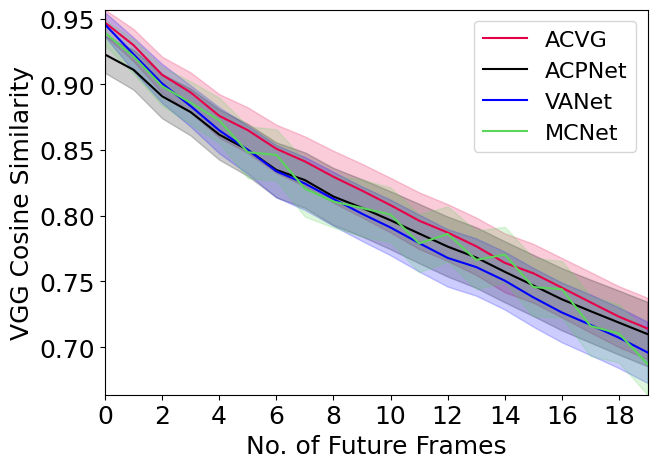
(a)

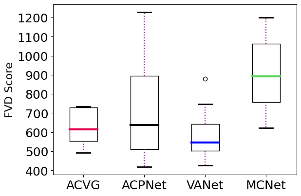
(b)

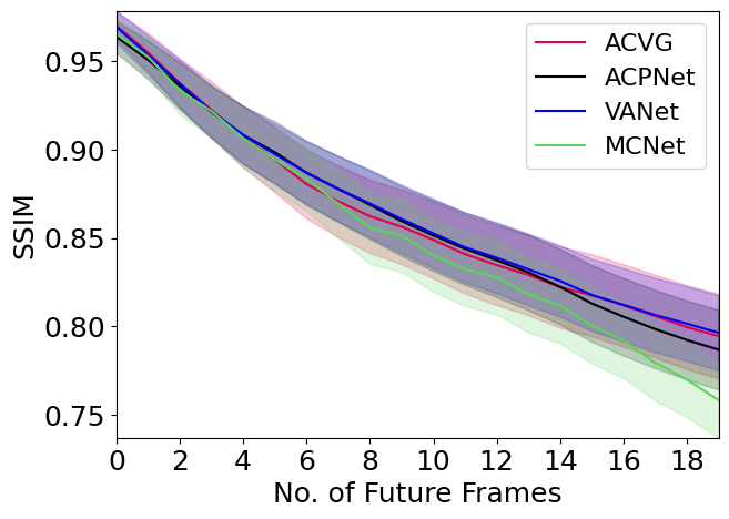
(c)

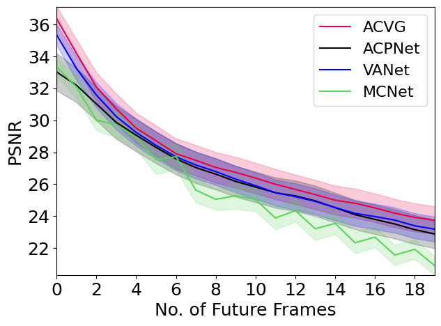
(d)

Figure 4: A Frame-wise quantitative analysis of ACVG, ACPNet, VANet and MCNet on RoAM dataset for predicting 20 frames into the future based on the past history of 5 frames. Starting from the left, we have plotted the mean performance index for VGG 16 Cosine Similarity (higher is better), FVD score (lower is better), SSIM (higher is better) and PSNR (higher is better) on the test set.

It can be noted in Eq. 20 that in order to evaluate the reconstruction penalty, we have calculated the $L^{1}$ loss between the ground truth image $x_{t}$ and predicted image $\tilde{x}_{t}$ but also the spatial gradient loss [villegas],[sarkar2021],[acpnet2023] between the two. The same is also followed for flow maps $o_{t}$ and $\tilde{o}_{t}$ in Eq. 21. The reconstruction penalty for the action likelihood function is calculated as follows with $\lambda_{a}=2$:

$$\underset{\Theta_{A}}{\max}\sum_{t=1}^{T}\text{ln}p_{\Theta_{A}}(a_{t}|S_{0:t},a_{0:t-1})\equiv\underset{\Theta_{A}}{\min}\sum_{t=1}^{T}\left\lVert{a}_{t}-{\tilde{a}}_{t}\right\rVert^{\lambda_{a}}$$ (22)

Other than the likelihood loss expressed with Eqs. 18, 19, 20, 21 and 22, we also use a scaled generative adversarial loss $\mathcal{L}_{adv}$ similar to [mathieu]. Due to the averaging effects of the deterministic framework, this adversarial loss is added to the Generator loss given by Eq. 20 and Eq. 21 to reduce the blurring effects in the prediction and generate more realistic images [villegas],[sarkar2021]. Detailed expression for the adversarial loss along with a short description of the discriminator network is given in the Supplementary material.

Training Loop: The training process for the ACVG framework comprises three distinct phases: (I) Generator Training, (II) Actor Training, and (III) Dual Training. To train the Dual Generator Actor Network effectively, we initially focus on training the Generator network alone for $N_{g}$ number of iterations as shown in Fig. 3(a). During this initial generator training phase, we set $\beta=1$ and $\gamma=0$ in Eq. 19. Once the Generator network has reached an adequate level of proficiency in grasping the spatio-temporal dynamics inherent in the flow and image data, we freeze the network’s weights. It’s important to note that during the Generator training phase, we assume that all future control actions, denoted as $a_{1:T}$, remain constant and equal to the last observed control action at $a_{t=0}$, i.e., $a_{1:T}=a_{t=0}$.

Following the freezing of the Generator network’s weights, the Actor network is then trained for a specified number of iterations, denoted as $N_{a}$. During this Actor network training phase as depicted in Fig. 3(b), the frozen Generator network operates in inference mode, where predictions from the Actor network $\tilde{a}_{t+1}$ are conditioned on the predicted image flow state $\tilde{\chi}_{t+1}$ from the Generator network, as outlined in Equation Eq. 15. Throughout the Actor network training phase, we set $\beta=0$ and $\gamma=1$. Subsequently, once the Actor network has reached an adequate level of training, we transition to dual training mode, where both the Generator and Actor networks are trained together. In this dual training mode, we set $\beta=1$ and $\gamma=1$. This dual training mode spans $N_{\text{dual}}$ iterations and is represented in Fig. 3(c). Observing Figure Fig. 3(c), it becomes apparent that in the dual training phase, a delayed actor-network is employed to provide the current action $\tilde{a}_{t}$ to the generator network. This design choice aligns with our utilization of a causal model, where the actor network generates the anticipated action $\tilde{a}_{t+1}$ grounded in the observation of state $\tilde{\chi}_{t+1}$. While tuning the hyperparameters $N_{g}$, $N_{a}$, and $N_{\text{dual}}$ is necessary, we found it manageable by monitoring individual reconstruction losses from the generator and actor networks.

3 RoAM dataset and Experimental Setup

We use Robot Autonomous Motion or RoAM dataset [acpnet2023] to test and benchmark The ACVG against 4 other state-of-the-art frameworks: ACPNet, VANet and MCNet due to the availability of the synchronised control action data along with the image frames. There are multiple partially observable datasets available in the literature [acpnet2023], however, RoAM is the only dataset that provides the synchronized control action data along with the image frames to properly test our hypothesis. Following the training process described in Section 2.3, ACVG is trained on the RoAM dataset using the ADAM optimizer [adam] with an initial learning rate of 0.0001 and a batch size of 8. The RoAM is an indoor human motion dataset, collected using a custom-built Turtlebot3 Burger robot. It consists of 25 long synchronised video and control-action sequences recorded capturing corridors, lobby spaces, staircases, offices and laboratories featuring frequent human movement like walking, sitting down, getting up, standing up etc. The dataset consists of almost 38,000 stereo image pairs along with the 2-dimensional control action vector stored in a .txt format. We split the dataset into training and test sets with a ratio of 20:5, respectively.

During the first phase of the training, the Generator network was trained on the entire training dataset for 1000 epoches for generating the pre-training weights as depicted in Fig. 3(a). Once the pre-traiing is done, we freeze the weights of the generator network and train the Actor network with Generator in the inference mode (Fig. 3(b)). We pre-train the Actor network on the full training dataset for 500 Epochs. Once we have the pre-training weights for both the Generator and Actor, we train both the networks in dual mode (Fig. 3(c)) for the next 1000 epochs. During both training and testing, each of the 25 video sequences was divided into smaller clips of 50 frames. A gap of 10 frames was maintained between each clip to ensure independence between two consecutive image sequences.

The dimension of the control action data $m=2$ as RoAM is recorded with a non-holonomic Turtlebot3 that has only two actuator actions for controlling 3 degrees of freedom: ($x,y$ and yaw). The available two control actions are the forward velocity along the $x$-coordinate of the robot’s body frame and the rotational rate or turn rate about the body $z$- axis. The forward velocity is within the range: $[0,0.1]$ m/s and the rotational rate is within $[-1.8,1.8]$ rad/sec. As described in Section 2, we use the normalised values of the action data to train ACVG framework.

The network was trained to predict 10 future frames based on the past 5 image frames of size $128\times 128\times 3$ and the corresponding history of control actions. During inference, the ACVG framework generates 20 future frames while conditioning on the last 5 known image frames and their corresponding action sequences. To evaluate the performance of ACVG compared to other state-of-the-art architectures for partially observable scenarios, we have also trained ACPNet, VANet and MCNet using the ADAM optimizer with similar hyperparameters as described in [sarkar2021], [acpnet2023], [Denton]. Each of these networks was trained for 150,000 iterations on a GTX 3090 GPU-enabled server as mentioned in [sarkar2021] and [acpnet2023].

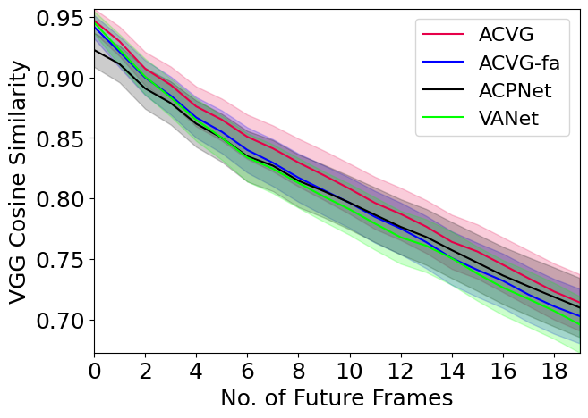
(a)

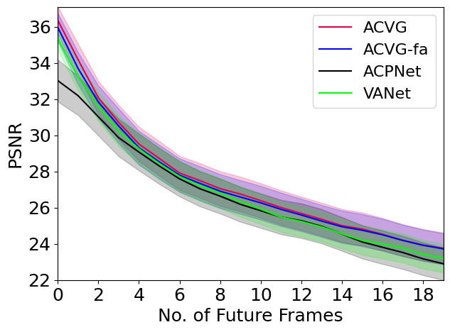
(b)

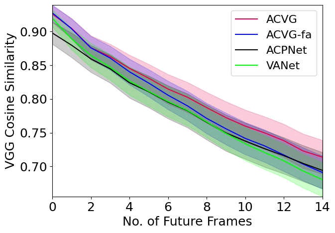
(c)

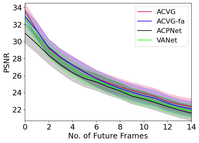
(d)

Figure 5: A Frame-wise ablation study with quantitative analysis of ACVG, ACVG-fa, ACPNet and VANet on RoAM dataset. Fig. 5(a): VGG 16 Cosine Similarity (higher is better) and Fig. 5(b): PSNR index (higher is better) for predicting 20 frames into the future from past 5 frames. Here the sampling interval between train and test time is same. Fig. 5(c): VGG 16 Cosine Similarity and Fig. 5(d): PSNR index for predicting 15 frames into the future from past 5 frames. Here the sampling interval at test time is twice the sampling interval at train time .

4 Results and Discussion

To conduct a quantitative analysis of the performance, we employed four evaluation metrics: Peak Signal-to-Noise Ratio (PSNR), Structural Similarity (SSIM), VGG16 Cosine Similarity [VGG16], and Fréchet Video Distance (FVD) [FVD]. Among these metrics, FVD measures the spatio-temporal perturbations of the generated videos as a whole, with respect to the ground truth, based on the Fréchet Inception Distance (FID) that is commonly used for evaluating the quality of images from generative frameworks. For frame-wise evaluation, we provided comparative performance plots for VGG16 cosine similarity index, SSIM, and PSNR. The VGG16 cosine similarity index measures the cosine similarity between flattened high-level feature vectors extracted from the VGG network [VGG16], providing insights into the perceptual-level differences between the generated and ground truth video frames. The VGG cosine similarity has emerged as a widely adopted standard for evaluating frame-wise similarity in the vision community, as seen in works like [Denton] and [villegasNeurIPS2019]. Its popularity stems from its capability to gauge structural similarities within the feature space rather than relying on raw images, which can pose challenges, particularly when one of the compared images is blurred. Nevertheless, we have included comparative plots for standard similarity and noise indexes, such as PSNR and SSIM, which have been extensively utilized in the literature.

Quantitative Evaluation: The figures presenting the quantitative performance metrics for VGG16 similarity, Fréchet Video Distance (FVD) score, Structural Similarity Index (SSIM), and Peak Signal-to-Noise Ratio (PSNR) are displayed in Figure 4. Here we have plotted the comparative performance among ACVG, ACPNet, VANet and MCNet. Notably, a lower FVD score indicates superior performance, whereas higher values for the remaining three metrics are indicative of better performance. The performance plots of VGG16 cosine similarity in fig 4(a) clearly indicate that ACVG performs much better than, ACPNet, VANet and MCNet. However, we see a marginal performance improvement over ACPNet. The VGG16 cosine similarity plot for MCNet in Fig. 4(a) clearly shows how MCNet struggles to capture the complex spatio-temporal dynamics embedded in the data due to its very small parametric space. Figure 4(a) illustrates that at the initial time step ($t=1$), both VANet and ACVG commence with the same similarity index. However, as time progresses, VANet experiences a gradual rise in prediction error, attributed to the compounding effect of accumulated errors from previous time steps. It is also worth noting that the parametric space for VANet is almost twice the parametric space of ACVG. A similar observation is also apparent from the performance plots of SSIM similarity and PSNR index, as depicted in Figure 4(c) and Figure 4(d), respectively.

The comparative performance analysis between ACVG and ACPNet, as depicted in Fig. 4(a), Fig. 4(b), Fig. 4(c), and Fig. 4(d), undeniably highlights the advantages of approximating the dual image and action pair dynamics, as outlined in Equations Eq. 12 and Eq. 17, within the ACVG framework. Interestingly Fig. 4(b) reveals that VANet outperforms ACVG by a marginal amount only in the case of the FVD score. This is attributed to the the much larger parametric space of the VANet architecture compared to ACVG which in turn lead to more realistic predictions. However, more realistic predictions does not guarantee the accurate estimation of the movement of the objects in the frame which in this case is supported by our comparative plots Fig. 4(a), Fig. 4(c), and Fig. 4(d). In the case of the FVD scores both, both ACVG and VANet networks generate a mean score below 650. Whereas for ACPNet the mean FVD score is slightly above 700 and for MCNet it is above 900.

We have conducted ablation study with ACVG, ACVG with fixed action (ACVG-fa), ACPNet and VANet and reported the quantitative plots in Fig. 5. ACVG-fa does not learn the action dynamics with an actor-network and simply considers the action of the robot to be constant during its inference phase from $t=1$ to $T$ meaning $a_{1:T}=a_{t=0}$. The training of ACVG-fa only consists of the Generator training phase of ACVG as depicted in Fig. 3(a). We also considered 2 different testing scenarios to better understand the effects of learning the dual interplay between the action of the robot and the generated image frames. In scenario one, we test the networks with the sampling interval $\Delta t_{\text{test}}$ between two consecutive image frames same as the sampling interval at train time $\Delta t_{\text{train}}$, i.e. $\Delta t_{\text{test}}=\Delta t_{\text{train}}$. The plots for VGG16 cosine similarity and PSNR for prediction of 20 future frames from 5 past frames are given in Fig. 5(a) and Fig. 5(b) respectively. In the second scenario the test sampling interval $\Delta t_{\text{test}}$ is twice the train sampling interval, i.e $\Delta t_{\text{test}}=2\times\Delta t_{\text{train}}$. The VGG16 cosine similarity and PSNR for prediction of 15 future frames from 5 past frames are given in Fig. 5(c) and Fig. 5(d) respectively. From the plots of VGG cosine similarity in Fig. 5(c) and Fig. 5(c) we can easily observe that ACVG outperforms all the 3 frameworks with a significant margin. More interestingly we can observe that in case Fig. 5(c), we can observe that both ACVG and ACVG-fa start from the same point but as time progresses, ACVG-fa’s performance degrades and it behaves more like ACPNet. In the PSNR index plots in Fig. 5(b) and Fig. 5(d), the mean trajectory of ACVG and ACVG-fa are almost indistinguishable since their generator architecture is almost similar, making their noise profiles almost same.

	t=1	t=3	t=5	t=7	t=9	t=11	t=13	t=15	t=17	t=21
Ground Truth
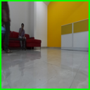
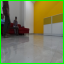
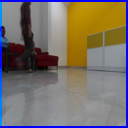
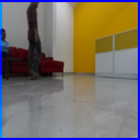
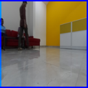
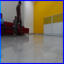
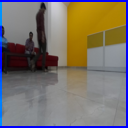
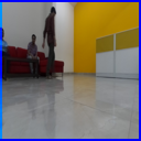
			ACVG
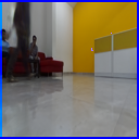
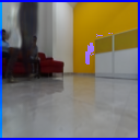
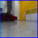
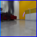
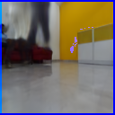
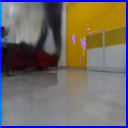
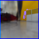
			ACPNet
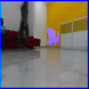
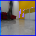
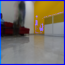
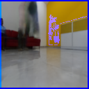
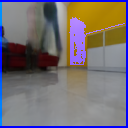
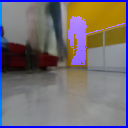
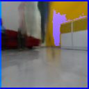
			VANet
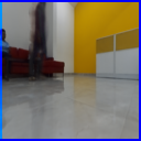
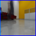
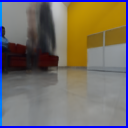
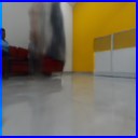
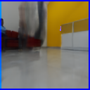
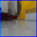
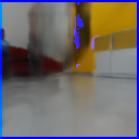
			MCNet

Figure 6: Predictions on partially observable RoAM dataset by ACVG, ACPNet, VANet and MCNet. The models were trained using 5 input-action frames to predict the next 10 frames. During the inference phase, the predicted frames were increased to 20.

Qualitative Evaluation: Figure 6 contains examples of raw video frames from the test set, generated by ACVG, ACPNet, VANet, and MCNet along with the first row representing the ground truth. Upon close observation of the image frames presented in Figure 6, it becomes apparent that the predicted frames from ACPNet and VANet have significant artefact errors compared to ACVG. This can be easily noticed from Fig. 6 at time-step $t=7,15,17,\text{ and }21$ for ACPNet and in the case of VANet the artefacts are prominently present at timestep $t=15,17,\text{ and }21$. From a close observation of the gait of the human motion at $t=17\text{ and }21$, we can clearly see how ACVG does a much better job at approximating the motion of the human figure compared to the other two. Fig. 6 also shows how MCNet fails to infer the gait of the human motion from the past image frames supporting our previous quantitative analysis in Fig. 4. Additional plots and raw predicted frames can be found in the Supplementary material.

5 Conclusion

A new video prediction framework capable of generating multi-timestep future image frames in partially observable scenarios has been presented. Our proposed framework ACVG explored learning the interplay of dynamics between the observed image and robot action pair with its dual Generator Actor architecture. Our detailed empirical results, clearly report that modelling the dynamics of control action data based on image state information yields superior approximations of predicted future frames. Notably, ACVG establishes a causal link between two distinct data modalities: the low-dimensional control action data $a_{t}$ from the robot and the high-dimensional observed image state $x_{t}$. This connection can potentially find applications in frameworks, such as reinforcement learning.