What Are the Odds? Improving the foundations of Statistical Model Checking

Abstract

Markov decision processes (MDPs) are a fundamental model for decision making under uncertainty. They exhibit non-deterministic choice as well as probabilistic uncertainty. Traditionally, verification algorithms assume exact knowledge of the probabilities that govern the behaviour of an MDP. As this assumption is often unrealistic in practice, statistical model checking (SMC) was developed in the past two decades. It allows to analyse MDPs with unknown transition probabilities and provide probably approximately correct (PAC) guarantees on the result. Model-based SMC algorithms sample the MDP and build a model of it by estimating all transition probabilities, essentially for every transition answering the question: “What are the odds?” However, so far the statistical methods employed by the state of the art SMC algorithms are quite naive. Our contribution are several fundamental improvements to those methods: On the one hand, we survey statistics literature for better concentration inequalities; on the other hand, we propose specialised approaches that exploit our knowledge of the MDP. Our improvements are generally applicable to many kinds of problem statements because they are largely independent of the setting. Moreover, our experimental evaluation shows that they lead to significant gains, reducing the number of samples that the SMC algorithm has to collect by up to two orders of magnitude.

1 Introduction

Markov decision processes (MDPs) [55] are the classic modelling formalism for dynamic systems with probabilistic and nondeterministic behaviour. Intuitively, MDPs comprise several states and each state has an associated set of available actions to choose from. In order to capture the aleatory uncertainty (the randomness of the process, e.g. a coin toss), each action corresponds to a distribution on the successor states rather than a single successor. The system evolves from a state by choosing an action, moving to a successor sampled from the corresponding distribution, and repeating this process. However, there also may be epistemic uncertainty [12] (the lack of knowledge, e.g. unknown bias of a coin), corresponding to these distributions being unknown. Traditionally, verification procedures assume full knowledge of the MDP, i.e. no epistemic uncertainty. This assumption is often unrealistic in practice; hence, over the past two decades, there has been an increasing interest in reliable analysis of MDPs where the exact transition probabilities are unknown.

Statistical model checking (SMC), see e.g. [45, 3, 49], is one of the approaches commonly employed to deal with unknown systems. Its main principle is to run simulations of the system and subsequently conclude properties of the system with statistical confidence. The strongest guarantees typically given in such a setting take the form of probably approximately correct (PAC) results: These depend on a confidence threshold $\delta$ and a precision $\varepsilon$ and guarantee that probably, i.e. with probability greater than $1-\delta$, the result is approximately correct, i.e. at least $\varepsilon$-precise. When considering discounted or finite-horizon objectives, the distance between the estimated result and the true value can be upper-bounded for paths of a certain length. Thus, PAC-guarantees and even bounds on sample-complexity can be derived in a straightforward manner, see e.g. [1, 43, 40, 57, 63, 67].

Our focus lies in giving PAC-guarantees for infinite-horizon objectives, where more involved methods have to be applied. Here, the first approaches used “model-free” SMC [22, 35], intuitively meaning that they do not construct a full representation of the model internally. While this works in theory, [35] requires knowledge of the mixing time of the MDP (which is as hard to compute as the value), and [22] needs an astronomical number of samples to provide non-trivial bounds, see [8, Sec. 4]. In contrast, model-based approaches have shown practical applicability [8, 65, 2, 60, 11, 54]. They estimate every transition probability to construct a model of the system; on this model, traditional verification methods can be applied. This SMC variant is able to give PAC-guarantees in many different settings, including stochastic games [8], multiple objectives [65], continuous-time [2], and continuous-space [11], often solving models with tens of thousands of transitions. Although improving the scalability and practical applicability was a declared goal of several of these papers and they developed and employed new heuristics [8, 2, 11], so far the underlying statistical methods overlook some seemingly straightforward, but high-impact improvements.

Our Contribution is to practically improve model-based statistical model checking. Colloquially speaking, for each transition in the MDP, we aim to answer the question: “What are the odds?” To this end, we propose methods that allow us to estimate transition probabilities more precisely than the state of the art based on the same data collected through simulations. Our methods have essentially no drawback, as they come at practically no computation-time overhead and, more importantly, never make the estimates worse. On the other hand, they improve upon existing methods by “making the most of the data”. Our improvements, provided by stronger statistical methods and structural analysis, are fundamental in the sense that they are (nearly) universally applicable and largely independent of the setting.

Concretely, there exist several variants of SMC, depending on the assumptions about the unknown MDP. Firstly, one can assume different knowledge settings, see [8, Def. 2]: Either we know at least the topology of the underlying graph of the MDP (called grey-box) or even that has to be inferred from the simulations (called black-box). Our methods are applicable in both settings, as we detail in Rem. 2.

Secondly, one can assume different ways to obtain samples from the MDP. From least to most restricted, these are: being able to sample any state-action pair, e.g. [71, 35], running simulations through the system that can only be restarted in the initial state, e.g. [22, 8, 2, 60], or batch learning, e.g. [48, 57, 69], where we have no control over which states are sampled but only get a fixed data set of past interactions.

Our methods are agnostic of the sampling method and just “make the most of the data” they get.

Thirdly, one can consider MDPs with various objectives. Most of our improvements are independent of the objective at hand. For the few that do utilise information about the objective, we sketch how to generalise them.

Lastly, our methods can also be useful for other approaches that are not model-based SMC aiming for PAC-guarantees. Essentially, any method that estimates transition probabilities can benefit from our insights, for example the reinforcement learning algorithms in [13, 69].

We mention a further direction of related work: algorithms with weaker guarantees than PAC. The (model-free) approach of lightweight scheduler sampling [50, 30, 29] only guarantees that the value is close to the optimum if good strategies are frequent, and, in any case, only provides one-sided bounds. The reinforcement learning algorithms in [69] guarantees an improvement over the policy that is used for obtaining the samples. The model-free reinforcement learning approach of [38, 39] does not give any guarantee on the result. These and our paper work in a setting where we are allowed to obtain samples from any part the unknown system, even unsafe states. In contrast, in a “safe online” setting, a good policy has to be computed while executing the system, and unsafe states have to be avoided. Here, we refer to works on PAC online learning [46, 44], shielding [6], and regret minimization [63].

Outline.

In Sec. 3, we provide an extensive survey of methods for estimating categorical distributions, the core task that is executed on every state-action pair of the MDP. Our survey includes the methods used in the verification community (e.g. [8, 11]) as well as from the literature on concentration inequalities [21] and statistics [4, 23, 64].

In Sec. 4, we show how to utilise the knowledge we have about the MDP and the property of interest. These optimizations allow us to invest less or even no part of our confidence budget $\delta$ for certain state-action pairs.

In Sec. 5, we empirically evaluate the impact of these improvements. We conclude that (i) our methods always have a positive impact, reducing the number of samples necessary to achieve a given precision $\varepsilon$; and (ii) in many cases this impact is quite significant, reducing the number of samples by up to two orders of magnitude.

2 Preliminaries

A probability distribution over a countable set $X$ is a mapping $d:X\to[0,1]$, such that $\sum_{x\in X}d(x)=1$. The set of all probability distributions on $X$ is $\mathcal{D}(X)$. For a set $S$, we denote by $S^{*}$ (or $S^{\omega}$) the set of all (in)finite sequences of elements of $S$.

2.1 Markov Decision Processes

A Markov decision process (MDP), e.g. [55], is a tuple $\mathcal{M}=(S,A,\mathsf{P})$, where $S$ is a finite set of states; $A$ is a finite set of actions, overloaded to yield for each state $s\in S$ a non-empty set of available actions ${A}(s)\subseteq A$; and $\mathsf{P}:S\times A\to\mathcal{D}(S)$ is the (partial) transition function, that yields for each state $s\in S$ and $a\in{A}(s)$ the associated distribution over successor states $\mathsf{P}(s,a)$. For ease of notation, we write $\mathsf{P}(s,a,s^{\prime})$ instead of $\mathsf{P}(s,a)(s^{\prime})$ and for a transition (state-action-state triple) $t=(s,a,s^{\prime})$ we write $t\in\mathsf{P}$ to say that $\mathsf{P}(s,a,s^{\prime})>0$.

The semantics of MDPs are defined in the usual way by means of paths, strategies and the probability measure in the induced Markov chain. We briefly recall this here and refer to [14, Chap. 10] for an extensive introduction. In the following, let $\mathcal{M}$ denote an MDP.

An infinite path is a sequence of state action pairs $\rho=s_{1}a_{1}s_{2}a_{2}\cdots\in(S\times A)^{\omega}$ with $\mathsf{P}(s_{i},a_{i},s_{i+1})>0$. Finite paths are finite prefixes of infinite paths, ending in a state. We denote by $\rho(i)$ the $i$-th state $s_{i}$ in a given path and by $\mathsf{Paths}_{\mathcal{M}}$ the set of all infinite paths.

A (memoryless deterministic, MD) strategy is a mapping $\pi:S\to A$, choosing one enabled action in each state, i.e. $\pi(s)\in A(s)$.

We write $\Pi_{\mathcal{M}}^{\mathsf{MD}}$ to refer to all MD strategies. Complementing an MDP with such a strategy and an initial state ${\hat{s}}\in S$ yields a Markov chain that induces a unique probability measure $\mathsf{Pr}_{\mathcal{M},{\hat{s}}}^{\pi}$ over infinite paths [14, Sec. 10.1].

An objective formalises the goal of the MDP. For simplicity, we focus on reachability, and in Rem. 1 explain how our methods are applicable to other objectives as well. Intuitively, a reachability objective is concerned with the probability of reaching a given set of goal states $T$. Define $\Diamond T\coloneqq\{\rho\in\mathsf{Paths}_{\mathsf{M}}\mid\exists i.\leavevmode\nobreak\ \rho(i)\in T\}$ as the set of paths that eventually reach $T$. The value of a state in an MDP is the maximum probability to achieve the objective, i.e. reach the goal states, under any strategy. Formally, the value of state $s$ is defined as $\mathsf{V}_{\mathcal{M}}(s)\vcentcolon=\max_{\pi\in\Pi_{\mathcal{M}}^{\mathsf{MD}}}\mathsf{Pr}_{\mathcal{M},s}^{\pi}[\Diamond T]$. (Note that MD strategies are sufficient to maximise the probability [14, Lem. 10.102].)

Finally, we recall the definitions of two important graph theoretic notions: strongly connected components and end components. A non-empty set of states $C\subseteq S$ in an MDP is strongly connected if for every pair $s,s^{\prime}\in C$ there is a non-empty finite path from $s$ to $s^{\prime}$. Such a set $C$ is a strongly connected component (SCC) if it is inclusion maximal, i.e. there exists no strongly connected $C^{\prime}$ with $C\subsetneq C^{\prime}$. SCCs are disjoint, so each state belongs to at most one SCC.

By $\operatorname{SCC}(\mathcal{M})$ we denote the set of SCCs of $\mathcal{M}$ which can be determined in linear time  [61].

A pair $(T,B)$, where $\emptyset\neq T\subseteq S$ and $\emptyset\neq B\subseteq\bigcup_{s\in T}{A}(s)$, is an end component of an MDP $\mathcal{M}$ if (i) for all $s\in T,a\in B\mathbin{\cap}{A}(s)$ we have $\{s^{\prime}\mid\mathsf{P}(s,a,s^{\prime})>0\}\subseteq T$, and (ii) for all $s,s^{\prime}\in T$ there is a finite path $\varrho=sa_{0}\dots a_{n}s^{\prime}\in(T\times B)^{*}\times T$, i.e. the path stays inside $T$ and only uses actions in $B$. Intuitively, an end component describes a set of states for which a particular strategy exists such that all possible paths remain inside these states.

An end component $(T,B)$ is a maximal end component (MEC) if there is no other end component $(T^{\prime},B^{\prime})$ such that $T\subseteq T^{\prime}$ and $B\subseteq B^{\prime}$. The set of MECs is denoted by $\operatorname{MEC}(\mathcal{M})$ and can be computed in polynomial time [27].

2.2 Statistical Model Checking

In this work, we consider the case where we do not know all details of the MDP in question, but rather only have sampling access. This means that for every state-action pair $(s,a)$, we do not know the corresponding probability distribution $\mathsf{P}(s,a)$, but we can obtain (arbitrarily many) samples drawn from it. Moreover, for our structural improvements in Sec. 4, we assume knowledge of the topology, i.e. that for every distribution $\mathsf{P}(s,a)$ we know its support $\{s^{\prime}\mid\mathsf{P}(s,a,s^{\prime})>0\}$. This is also called grey-box setting [8, 2], as opposed to the completely opaque black-box [28, 8]. We discuss in Rem. 2 how our methods can be applied in the latter setting.

To solve such unknown systems, statistical model checking (SMC) is employed. In this section, we recall model-based SMC, the approach we mainly aim to improve. For an overview of other methods related to SMC, we refer to Sec. 1.

Example 1

Consider the simple MDP in Fig. 1 which represents throwing a (potentially biased) six-sided die. The initial state ${\hat{s}}$ has only a single action $\mathsf{throw}$ that leads to one of six possible successors. We do not know the precise transition probabilities $p_{1},\ldots,p_{6}$ for each side but rather have to estimate them. More formally, we want to estimate the probability distribution $\mathsf{P}({\hat{s}},\mathsf{throw})$ based on a finite sequence of samples, i.e. throwing the die several times and recording the outcome. For example, throwing the die five times might yield the sequence $(\text{\faDiceTwo},\text{\faDiceSix},\text{\faDiceThree},\text{\faDiceFour},\text{\faDiceThree})$.

Due to the statistical nature of the problem, it is impossible to give non-trivial hard guarantees. For example, even if the die showed every time in a million rolls, there is an (abysmally small) non-zero chance that this was just “bad luck” and the die is, e.g., uniform. Similarly, it is also impossible to give precise values in general. Thus, instead we aim for probably approximately correct estimates.

Concretely, given the sequence of samples above and a confidence threshold $\delta=0.1$, we can employ Hoeffding’s inequality (described in more detail in Sec. 3) to conclude that the probability $p_{1}$ of throwing a is between $0$ and $0.55$. We have the statistical guarantee that this statement is true with at least probability $\delta=0.1$; in other words, the chance that $p_{1}>0.55$ and we were just very unlucky to not see any in our samples is below $0.1$. The inferred interval $[0,0.55]$ is called confidence interval and, by increasing either the number of samples or the confidence threshold $\delta$, we can decrease its width and make our estimates more precise.

Figure 1: A six-sided die modelled as a (simple) Markov decision process.

SMC-Algorithm Structure.

Algorithms for model-based SMC, e.g. [8, 65, 2, 60, 11], work in two phases: First, they obtain a finite number of samples from the MDP and estimate transition probabilities based on these samples. If these estimates are precise enough to prove the property, the algorithm terminates. Otherwise, it returns to the first phase. Thereby, it obtains more samples, can estimate the transition probabilities more precisely, and eventually terminates. Our work focusses only on the second phase: Given a finite number of samples, what is the best way to estimate transition probabilities, colloquially “making the most of the data”.

Note that we might not yet have enough samples to make the interval on the value or on the probabilities $\varepsilon$-precise. Thus, we only aim to make these intervals “as small as possible” given the data at our disposal. We do not explicitly ask for the minimum interval size, because we cannot exclude the future development of other statistical methods that yield more precise intervals. By reducing the width of the intervals in the second phase of the algorithm, we get more precise estimates from the samples, and thus we also improve the performance of the overall SMC-algorithm.

Usually, the problem that SMC aims to solve is Property-SMC: Given sampling access to an MDP and an objective, we want to estimate the value. In our example, this may be the probability of rolling an even number, i.e. reaching $T=\{\text{\faDiceTwo},\text{\faDiceFour},\text{\faDiceSix}\}$. We require that the estimate is probably approximately correct (PAC), i.e. $\varepsilon$-close to the true value with probability at least $1-\delta$. In the following, we also consider a related problem, namely Model-SMC. There, we want to learn all probabilities occurring in the model up to a given precision $\varepsilon$. In our example, this corresponds to learning $p_{1},\ldots,p_{6}$. The problems are related because for providing bounds on a property, we also need to estimate the transition probabilities. However, they are also different: On the one hand, even if all transition probabilities are $\varepsilon$-precise, the estimate for the value might be less precise; on the other hand, we might not need to estimate every transition probability in order to give bounds on the value.

SMC-algorithms want to use as few samples as possible to return a result with the given precision $\varepsilon$. We formalise this as the Probability Sample Complexity Problem in Sec. 3.3 and use this viewpoint in our experiments. The rest of the paper considers the (equivalent) dual problem of reducing the interval size based on given data:

State-of-the-art.

We now recall the state-of-the-art methods used to solve our problems. We first discuss Model-SMC, where we are interested in estimating all transition probabilities as precisely as possible. For this, the confidence budget $\delta$ is uniformly distributed over all transitions, and Hoeffding’s inequality is applied (detailed in Sec. 3.2) to get a confidence interval for each of them. Every transition then has a probability of at least $1-\frac{\delta}{\lvert\mathsf{P}\rvert}$ to be correct, where $\lvert\mathsf{P}\rvert$ is the number of transitions. Using the union bound, the probability of all transition being correct is greater than $1-\delta$, which is the goal.

We briefly comment on the few cases in verification literature where methods other than Hoeffding’s inequality were applied to improve the precision of the estimates; further details can be found in Sec. 0.A.4: [16] introduced the “Chen bound”, but it is unclear how it was derived from literature and whether it is correct. [60] uses linearly updating intervals, but this precludes giving PAC-guarantees. [11] developed a new scenario-based approach and we prove that it is in fact a weaker version of the (well-known in statistics) Clopper-Pearson Interval, which we discuss later.

To solve Property-SMC, all of the works [8, 65, 2, 60, 11] essentially first solve Model-SMC, i.e. estimate all transitions as precisely as possible. Then, they complement the given MDP with the resulting confidence intervals, constructing an interval MDP [36]. Solving this interval MDP yields bounds on the value of the given MDP.

Remark 1

Note that Model-SMC does not depend on an objective and Property-SMC only requires objective-specific reasoning when solving the interval MDP. Thus, almost all our methods for decreasing the number of samples are applicable independently of the objective. For the only exception, the objective-specific improvements in Sec. 4.2, we explain how they can be generalised.

3 Statistical Methods for Estimating Probabilities

To solve Model-SMC or Property-SMC in a model-based fashion, it is necessary to estimate transition probabilities from samples. This section presents methods to estimate the distribution $\mathsf{P}(s,a)$ for a single state-action pair $(s,a)$ in the given MDP. In Sec. 3.1 we discuss estimating the whole distribution (the whole die) at once. In Sec. 3.2 we detail how to estimate a single transition probability $\mathsf{P}(s,a,s^{\prime})$; this essentially views the samples drawn from $\mathsf{P}(s,a)$ as a coin toss, either reaching the successor $s^{\prime}$ or not. We survey the literature, including methods used in verification, the concentration inequalities from [21] applicable in our setting, and methods from statistics literature [4, 23, 64]. Finally, Sec. 3.3 compares the methods.

3.1 Estimating a Die

In the context of Markov systems, there are two common approaches to estimate a probability distribution based on samples: Firstly, state-of-the-art model-based SMC algorithms split the confidence budget among the transitions and compute a confidence interval for each transition probability individually using a method from Sec. 3.2.

The other approach, used by, e.g., MBIE [59] and UCRL2 [10], computes a maximum likelihood estimate of the probability distribution, i.e. the empirical average of each outcome; then, it constructs the confidence region as an $L^{1}$-ball around this estimate; in other words, the confidence region contains all probability distributions whose $L^{1}$-distance from the empirical average is less than a certain precision. This precision depends on the number of samples and the number of successors [66].

The advantage of the $L^{1}$-ball is that theoretically it allows to account for the dependence between the transition probabilities, i.e. that $\sum_{i=1}^{k}p_{i}=1$. However, [69] shows that the method scales poorly with the number of successors of a state-action pair; thus, it is advantageous to transform the model and reduce this number for each state-action pair. When every state-action pair has two successors, the number of samples required to prove a property is minimised [68, App. A]. But then the method of [66] effectively coincides with applying Hoeffding’s inequality to each transition probability individually (see Sec. 0.A.1). As we show in Sec. 3.2, Hoeffding’s inequality is a sub-optimal way to estimate transition probabilities. Moreover, applying such an $L^{1}$-ball approach to the Model-SMC as defined it in Sec. 2.2 would be disadvantageous as it requires bounding the $L^{\infty}$-norm. Thus, in this work, we focus on the approach that estimates every transition probability individually.

3.2 Estimating a Coin

This section concerns the most basic problem in the whole SMC-pipeline: estimating a single transition probability $\mathsf{P}(s,a,s^{\prime})$ with given confidence budget $\delta$ (usually a small fraction of the whole budget). The relevant information from the samples are (i) how often was $(s,a)$ sampled and (ii) how often was the successor $s^{\prime}$ chosen. We view this as a binomial distribution where sampling $s^{\prime}$ is counted as a success. Throughout this section, we refer to a binomial distribution with success probability $p$ and a test sequence on it with $n$ trials and $k$ successes. We write $\hat{p}=\frac{k}{n}$ for the maximum likelihood estimate of $p$. Thus, the problem considered now is:

The probability $\mathop{\mathrm{Pr}}[\underline{p}\leq p\leq\overline{p}]$ for a specific $p$ is called the coverage probability of $p$. In our setting we require that it is consistently at least $1-\delta$ for all $p$. Many statistical methods either fail to provide a proper coverage probability for a small number of samples, or only provide an average coverage probability of $1-\delta$ when assuming $p$ to be uniform over $(0,1)$. These include the Wald interval [23, 64], the Wilson score interval without continuity correction [70, 23, 64], the Agresti-Coull interval [4], the Arcsine interval [23], and the Logit interval [23].

We now first detail the methods most suitable for the problem at hand, namely Hoeffding’s inequality, the Wilson score interval with continuity correction, and the Clopper-Pearson Interval. We summarise the important outcome of this description below in Theorem 3.1. Afterwards, we discuss further methods from the literature and why they are not preferable for solving the Probability Estimation Problem.

Theorem 3.1

Hoeffding’s inequality, the Wilson score interval with continuity correction, and the Clopper-Pearson Interval all solve the Probability Estimation Problem.

Hoeffding’s Inequality.

In his seminal paper [41] Hoeffding provides a confidence interval for the sum of random variables. Several works have applied this to estimate binomial distribution parameters by viewing the outcome each Bernoulli trial as a random variable $X_{i}$ with $X_{i}=1$ meaning a success, and otherwise $X_{i}=0$. Applying Hoeffding’s inequality results in the $1-\delta$ confidence interval $[\underline{p}_{ho},\overline{p}_{ho}]$ with $\underline{p}_{ho}=\min\{1,\hat{p}+c_{ho}\}$, $\overline{p}_{ho}=\max\{0,\hat{p}-c_{ho}\}$, and $c_{ho}=\sqrt{\ln(2/\delta)/2n}$.

While this result is often referred to as Hoeffding’s inequality, the original statement is much stronger, being applicable to any i.i.d. bounded random vector. As such, it is not too surprising that there are methods specifically tailored towards estimating binomial proportions that provide stronger bounds than Hoeffding’s inequality.

Wilson Score Interval and Continuity Correction.

One of the most famous and widely used (see [4, 23, 64]) methods is the Wilson score interval [70]. As mentioned previously, the Wilson score only guarantees that the average coverage probability is above the desired correctness probability $1-\delta$ [23].

Later works address this shortcoming and introduce a continuity correction (CC) for the Wilson score interval [53].

This variant then indeed achieves coverage of $1-\delta$ for all $p$ where the confidence interval $[\underline{p}_{wcc},\overline{p}_{wcc}]$ is computed as follows:

$$\underline{p}_{wcc} =\max\left\{0,{{\left(2n{\hat{p}}+z^{2}-z{\sqrt{z^{2}-{\tfrac{1}{n}}+4n{\hat{p}}(1-{\hat{p}})+(4{\hat{p}}-2)}}-1\right)}/{\left(2(n+z^{2})\right)}}\right\}$$

$$\overline{p}_{wcc} =\min\left\{1,{{\left(2n{\hat{p}}+z^{2}+z{\sqrt{z^{2}-{\tfrac{1}{n}}+4n{\hat{p}}(1-{\hat{p}})-(4{\hat{p}}-2)}}+1\right)}/{\left(2(n+z^{2})\right)}}\right\}$$

where $z$ is the $1-\frac{\delta}{2}$ quantile of the standard normal distribution.

Clopper-Pearson Interval.

Another widely used confidence interval method was introduced by Clopper and Pearson [26]. The approach inverts the task and, given $n$ and $k$, asks for the minimum (resp. maximum) $p$ such that observing at least (resp. at most) $k$ out of $n$ successes would have a probability of $1-\frac{\delta}{2}$. The resulting $1-\delta$ confidence interval can be represented in a closed form using the inverse regularised beta function $I^{-1}_{x}(a,b)$ [62] as $[\underline{p}_{cp},\overline{p}_{cp}]=[I^{-1}_{\delta/2}(k,n-k+1),I^{-1}_{1-\delta/2}(k+1,n-k)]$ for $0<k<n$. For the case $k=0$ (resp. $k=n$) the lower (resp. upper) bounds needs to be taken as 0 (resp. 1).

As the Clopper-Pearson interval was the first estimation interval for a binomial parameter achieving a coverage probability of at least $1-\delta$ for all $p$, it is often called the “exact” method. This name might be slightly misleading, as the coverage probability is not necessarily exactly $1-\delta$, but higher for many $p$.

Recently, a method for computing PAC probability intervals was proven in [11] based on previous results of [56]. Interestingly, we notice that their method produces a weaker version of the Clopper-Pearson interval, see Sec. 0.A.4 for details.

Further Confidence Methods.

Next, we want to briefly discuss several other confidence interval methods and reasons why we do not recommend to use them.

Bennett’s inequality [17] is very similar to Hoeffding’s inequality but additionally includes information about the variance of the random variable. This is an improvement when bounding the sum of random variables with known distributions, but a hindrance when it comes to the inversion of the problem since we now would also need to estimate the variance of the random variable. For a binomial variable, this is given as $p\cdot(1-p)$ and thus has a trivial upper bound of $\frac{1}{4}$. However, using this bound, Benett’s inequality effectively is always worse than Hoeffding’s inequality, as we prove in Sec. 0.B.1. There exist more recent methods that do estimate the variance from data and asymptotically outperform Hoeffding’s inequality [51], however only for $p$ away from $\frac{1}{2}$, and even then empirically only for large $n$.

Very closely related is Bernstein’s inequality [19] which is a conservative relaxation of Bennett’s inequality obtainable by replacing a term in Bennett’s inequality by a polynomial. While this eases inversion of the problem a lot, due to its conservativeness it provides strictly wider confidence intervals than Bennett’s inequality.

We also point out that Jeffrey’s interval [23] as a Bayesian method can give guarantees in a Bayesian sense by providing a credible interval. In this paper we avoid credible intervals as they rely on defining a prior distribution over $p$ which we cannot justify in a grey-box setting for general Markov systems. However, such Bayesian methods can be considered if prior distributions are known.

Lastly, there are methods providing $1-\delta$ coverage which we did not investigate here, such as the Blyth-Still(-Casella) interval [20, 24], inverted likelihood ratio test interval [5], or Duffy-Santner interval [32]. Summarizing the detailed discussion of [23], we conclude that generally these methods tend to deliver very similar results as the Wilson score interval with CC and the Clopper-Pearson interval with only slight differences, mostly in the way they ensure coverage for $p$ close to 0 or 1. Additionally, all these methods involve complex procedures that are not easily invertible and thus do not directly allow a computation of an a priori bound of the number samples required, which is the problem we address in Sec. 3.3. Because of this and the fact that Wilson’s and Clopper-Pearson’s methods are more popular and hence already implemented in a lot of statistical libraries, we do not consider them any further.

3.3 Sample Complexity of a Coin

While one could compare the different methods by fixing a set of samples, towards a theoretical analysis it is more instructive to invert the task and ask: How many samples are required to achieve a given precision $\varepsilon$? In the following, we address how to compute the worst-case sample number for the three main methods established above – Hoeffdings’s bound, Wilson score interval and Clopper-Pearson interval – and compare their sample complexities on single transitions. Later, we then use these results in our experiments Sec. 5 to evaluate the different methods on full MDPs.

At first glance, this problem is not easy to solve, since the width of the interval not only depends on the sample size $n$ and confidence threshold $\delta$, but also on the success rate $\hat{p}$ of samples. Fortunately, all three methods have in common that they maximise the interval size when $\hat{p}=\frac{1}{2}$. We prove the following lemma in Sec. 0.A.2.

Lemma 1 ()

Given a sequence $\mathcal{S}$ of $n$ samples from an unknown binomial distribution, and a confidence threshold $\delta\in(0,1]$, the confidence interval $[\underline{p},\overline{p}]$ computed by Hoeffding’s inequality, the Wilson score with CC, or the Clopper-Pearson interval maximises $\overline{p}-\underline{p}$ when $\mathcal{S}$ contains an equal amount of positive and negative samples.

Conversely, this means that the probability sample complexity problem can be solved by considering the worst-case $\hat{p}=\frac{1}{2}$. From here, the number of samples can be found using, e.g., a binary search on $n$. Note that, when estimating a distribution $\mathsf{P}(s,a)$ for a state-action pair (“a die”), the worst-case occurs when one of the successors $s^{\prime}$ has $\hat{p}=\frac{1}{2}$. As the samples drawn from $\mathsf{P}(s,a)$ are used for all successor states, all other states can be estimated with the necessary precision after $n$ samples, where $n$ is the solution of the probability sample complexity problem of $\mathsf{P}(s,a,s^{\prime})$.

Figure 2: Ratio of sample complexity for given $\delta$ (0.1 left and 0.001 right) and different $\varepsilon$ between Hoeffding bound, and Wilson score with CC (green) and Clopper-Pearson interval (orange), respectively.

In Fig. 2 we plot the ratio of samples required in the worst case between Wilson score with CC and Clopper-Pearson compared to the Hoeffding interval.

We plot ratios instead of absolute number of required samples, since the latter grow exponentially in the precision $\varepsilon$ (as can be seen by inverting the bounds in Sec. 3.2), making it hard to visualise the relative difference.

We observe that both Wilson score with CC as well as the Clopper-Pearson bound clearly outperform Hoeffding’s bound in all cases. The impact is biggest for large $\varepsilon$, with the Wilson score being superior. However, the most important values for practical applications are small precision requirements, e.g. $\varepsilon\leq 0.2$, for which we do not see a big difference between both methods and also notice that the exact value of $\varepsilon$ has very little impact.

Towards the impact of $\delta$, we see that in our two examples a smaller $\delta$ correlates with less improvement for small $\varepsilon$, however still all ratios are above 1, implying that both methods still require less samples than the Hoeffding bound. For the Wilson score with continuity correction, we provide a formalization this statement. Due to space constraints, the proof can be found in Sec. 0.A.2.

Lemma 2 ()

Let $n_{h}(\delta,\varepsilon)$ and $n_{w}(\delta,\varepsilon)$ be the solution to the probability sample complexity problem for a given confidence threshold $\delta$ and precision threshold $\varepsilon$ for the Hoeffding interval and the Wilson score with continuity correction, respectively. Then $r_{\delta}=\lim_{\varepsilon\rightarrow 0}\frac{n_{h}(\delta,\varepsilon)}{n_{w}(\delta,\varepsilon)}>1$ for all $0<\delta<1$ Further, $r_{\delta}>r_{\theta}$ iff $\delta>\theta$.

In further experiments (see Sec. 0.B.2), we considered other values than the worst case $\hat{p}=\frac{1}{2}$. In summary, we find that the Wilson score with CC is preferable for $\hat{p}$ close to $\frac{1}{2}$ whereas Clopper-Pearson produces smaller intervals for $\hat{p}$ close to $0$ or $1$.

To summarise this section, we conclude that both the Wilson score with CC and the Clopper-Pearson bound empirically outperform the Hoeffding bound, with the Wilson score doing so provably. We also mention that the relative difference in sample complexity is further emphasised for large $\epsilon$ and $\delta$. Whether the Wilson score and the Clopper-Pearson interval provides a better sampling complexity depends on $\hat{p}$, although their sample complexities are very similar for small $\varepsilon$.

4 Structural Improvements

As outlined before, even state-of-the-art SMC algorithms naively distribute the confidence budget among all transitions and estimate the probability for each of them. However, especially in the grey-box setting, we actually have a lot of structural information that we can utilise to improve estimates or even conclude that estimation is not even needed at all. In particular, we identify graph structures in the MDP that allow us to invest less or even no confidence budget at all. In Sec. 4.1, we explain how to use information about the model structure; these ideas are applicable to both Model-SMC and Property-SMC. In Sec. 4.2, we exploit the additional information about the property, which naturally is only applicable to the latter.

Remark 2 (Applicability in the Black-box Setting)

Recall that we assume grey-box setting, i.e. that for every distribution $\mathsf{P}(s,a)$ we know its support $\{s^{\prime}\mid\mathsf{P}(s,a,s^{\prime})>0\}$, which in turn gives the complete transition graph. In the black-box setting [28, 8], we do not know the support of any distribution, which is the main information we exploit in this section. Instead, we only have an upper bound on the minimum occurring transition probability $p_{\min}$. However, even given only that information, we can infer the topology using the methods from [28, 8]: Consider a distribution $\mathsf{P}(s,a)$. For every successor that we sample, we can compute confidence intervals on its probability. Intuitively, once the sum of all lower bounds of these confidence intervals is greater than $p_{\min}$, the probability that we have overlooked a successor is less than our confidence budget. Thus, from that point onward we know the support of $\mathsf{P}(s,a)$ with sufficient confidence and can apply structural improvements. We remark that in this phase the recommendations of Sec. 3 also help, since we get better confidence intervals and thus get to know the topology sooner than in previous works.

4.1 Using Information About the Model

Recall that in Model-SMC, our task effectively is to learn the set of all distributions in the model. We now present ideas to improve this general task.

Notably, in the following section, we then discuss how in Property-SMC distributions can be simplified or completely “eliminated”. The techniques of this section then also can be applied in this case, i.e. for distributions not directly appearing in the model.

Small Support.

Clearly, if a distribution only has a single successor, we can immediately conclude that the transition probability equals one

, trivially saving on confidence budget while also achieving full precision.

Moreover, if a distribution only has two successors, it suffices to estimate only one of the two probabilities: If we estimate $p_{1}\in\hat{p}\pm c$, we can immediately conclude that $p_{2}\in(1-\hat{p})\pm c$. Notably, the error bound for $p_{2}$ is the same as for $p_{1}$ and the confidence in the estimation of $p_{1}$ transfers to $p_{2}$: The estimation of $p_{2}$ is correct exactly when $p_{1}$ is correct. Thus, we only need to learn one transition probability instead of two, saving budget.

One might be tempted to apply this reasoning to general distributions: Clearly, if we have $k$ successors, we only need to estimate $k-1$ probabilities and the $k$-th follows from the rest. However, in this way, we get a worse error bound for the $k$-th estimate. For example, if we want to estimate a three-successor distribution and know that $p_{1}\in\hat{p_{1}}\pm c$ and $p_{2}\in\hat{p_{2}}\pm c$, we can only show $p_{3}\in(1-\hat{p_{1}}-\hat{p_{2}})\pm\textbf{2}\cdot c$. Hence we do not see an immediate way to extend this idea to more than two successors.

Independence.

By their very nature, the transition distributions in Markov systems are independent. Hence, instead of employing the union bound when estimating the overall error probability, when can multiplicatively divide up the confidence, as follows. Recall that ultimately we are interested in the probability of collectively estimating all probabilities of every distribution we are interested in correctly. More formally, let $\text{Corr}=\text{\leavevmode\ltxml@oqmark@open\textquotedblleft\penalty 10000\hskip-0.0002pt\hskip 0.0002ptAll transitions estimated correctly\textquotedblright\ltxml@oqmark@close{}}$ and require that $\mathop{\mathrm{Pr}}[\text{Corr}]\geq 1-\delta$. Observe that this event equals $\bigcap_{t\in\mathsf{P}}\text{Corr}(t)$, where $\text{Corr}(t)$ is the event that transition $t$ is estimated correctly. As explained in Sec. 2.2, the usual trick is to consider the complement of Corr and use the union bound, formally $\delta\leq 1-\mathop{\mathrm{Pr}}[\text{Corr}]=\mathop{\mathrm{Pr}}[\overline{\text{Corr}}]=\mathop{\mathrm{Pr}}[\bigcup_{t\in\mathsf{P}}\overline{\text{Corr}(t)}]\leq\sum_{t\in\mathsf{P}}\mathop{\mathrm{Pr}}[\overline{\text{Corr}(t)}]$.

Instead of splitting Corr individually by transitions, we propose to first split by state-action pairs, i.e. $\mathop{\mathrm{Pr}}[\text{Corr}]=\mathop{\mathrm{Pr}}[\bigcap_{(s,a)\in S\times A}\text{Corr}(s,a)]$, where $\text{Corr}(s,a)$ is the event that we correctly estimate the overall distribution $\mathsf{P}(s,a)$. Intuitively, we simply say that the probability of estimating everything correctly equals the probability of jointly for each distribution estimating every transition of that distribution correctly. Now, note that while the events $\text{Corr}(t)$ are not independent, $\text{Corr}(s,a)$ however are! Thus, we obtain that $\mathop{\mathrm{Pr}}[\text{Corr}]=\prod_{(s,a)\in S\times A}\mathop{\mathrm{Pr}}[\text{Corr}(s,a)]$.

To generalise, note that it is irrelevant that we talk about state-action pairs and their related distributions. Rather, suppose that we are interested in estimating each distribution in a given set of independent distributions $\mathcal{D}$, e.g. $\{\mathsf{P}(s,a)\mid(s,a)\in S\times A\}$, and define Corr as the event that we estimated all distributions correctly.

Lemma 3

For a set of independent distributions $\mathcal{D}$, we have $\mathop{\mathrm{Pr}}[\text{Corr}]\geq(1-\delta)^{1/\lvert\mathcal{D}\rvert}$.

While this restriction is strictly better, we note that it has diminishing effects for large number of distributions to be estimated or strong confidence requirements, i.e. $\delta$ close to $0$. In particular, we have that the difference of confidence requirements imposed on each distribution, i.e. $(1-\delta)^{1/n}$ and $1-\delta/n$, approaches zero for $\delta\to 0$ or $n\to\infty$. Dually, this also means that the effect is more prominent if we can weaken the confidence requirements for particular distributions or shrink $\mathcal{D}$ altogether, using e.g. our other presented methods.

4.2 Using Information About the Property

Now, we discuss optimizations specific to exploiting the structure of given systems relative to the given property. While the overall graph structure of the model is largely irrelevant for Model-SMC – after all, by definition of the problem there simply is no way around estimating each probability distribution individually – we can achieve significant gains in the context of Property-SMC. Concretely, we can combine insights about the objective with the transition structure to derive that the exact probability of some transitions actually is irrelevant to the value of the objective. For the remainder of this section, fix an MDP $\mathcal{M}$ and reachability objective $T$.

Equivalence Structures.

We first discuss ideas that allow us to completely ignore the probabilities of certain state-action pairs. Firstly, observe that we can determine states with value 1 or 0 through classical attractor-based graph analysis [34, Sec. 4]. For example, consider a state $s$ that has an action $a$ which transitions with probability 1 into the goal set $T$. Even if this state has several other actions, we can immediately derive the exact value of $s$ without committing any confidence budget for the other actions. Similarly, we can identify states which have zero probability.

Next, by similar reasoning, we can exclude every internal action inside MECs: Using well-known results [31, Thm. 3.1], we know that every state inside a MEC can reach any other state in it with probability 1, no matter what the actual transition probabilities are. Consequently, all states inside a MEC have the same value and we only need to estimate the probabilities of transitions actually leaving the MEC.

We formalise this claim by stating that for state-action pairs in a MEC, only the support of the distribution matters, not the actual probabilities. (See also [31, Alg. 3.3] for the related notion of MEC quotient.)

Lemma 4

For every EC $(T,B)$ and every $s\in T,a\in B\mathbin{\cap}{A}(s)$, the following holds: Changing $\mathsf{P}(s,a)$ to some alternative distribution $\mathsf{P}^{\prime}(s,a)$ with $\{s^{\prime}\mid\mathsf{P}(s,a,s^{\prime})>0\}=\{s^{\prime}\mid\mathsf{P}^{\prime}(s,a,s^{\prime})>0\}$ does not change $\mathsf{V}_{\mathcal{M}}(u)$ for any state $u\in S$.

The same holds true for state-action pairs in the attractor of a MEC, i.e. state-action pairs from which, once taken, we cannot avoid entering the MEC (formally, as we consider maximizing reachability objectives, the attractor of a set $U\subseteq S$ is the set computed by inputting $U$ in [31, Alg. 3.2]). Using this and [31, Thm. 3.7], we generalise the reasoning above which talked about attractors of goal and sink states.

Lemma 5

Let $(T,B)$ be an EC and $t\in T$. For every state $s$ in the attractor of $T$, we have $\mathsf{V}_{\mathcal{M}}(s)=\mathsf{V}_{\mathcal{M}}(t)$. Moreover, for $a\in{A}(s)$, we can alter $\mathsf{P}(s,a)$ as in Lemma 4 without changing $\mathsf{V}_{\mathcal{M}}(u)$ for any state $u\in S$.

Together, these lemmata allow us to avoid spending any confidence budget on states that are in the attractor of some MEC. To generalise this to other objectives, observe that the key idea is to find states which provably form an equivalence class w.r.t. the achieved value. So, while we only reason about reachability here, this idea naturally translates to, e.g., total reward or mean payoff, where ECs similarly form equivalence classes, see [15, 7].

Figure 3: Left: A small MDP. Right: “Compressed” MDP using fragment analysis. We omit transition probabilities, as these would also not be visible to our algorithm.

Fragments.

We propose to identify parts of the state space for which the “internal” behaviour is not interesting. For an illustrative example, consider the MDP depicted in Fig. 3 (left). The marked area of the state space has a lot of internal structure; however, when considering reachability, we actually only care about how we could leave this area. In this example, there are only two possibilities, namely through the actions $a$ or $b$ in state $s_{3}$. In other words, we only are interested in the “big step” behaviour of the system as depicted in Fig. 3 (right). So, once we identify this fragment, we only need to estimate two probabilities, namely the probability to reach $e_{1}$ under $a$ and $b$, respectively, instead of $>10$ distinct values. (Recall that the probability of leaving to state $e_{2}$ can be directly derived from the respective probability for $e_{1}$ using small support from Sec. 4.1.) Observe that if we had a second transition entering this area, we would need to estimate four probabilities.

Generally, for a set of states $R\subseteq S$, we can estimate either the internal behaviour, i.e. each transition probability individually, or for each pair of entry and internal strategy estimate the distribution over all exits, which we define as follows. A state $s\in R$ is called entry of $R$ if there exists a transition $(s^{\prime},a,s)\in\mathsf{P}$ with $s^{\prime}\notin R$ or if $s$ is the initial state. Similarly, $s\notin R$ is called exit of $R$ if there exists a transition $(s^{\prime},a,s)\in\mathsf{P}$ with $s^{\prime}\in R$.

Together, let In and Out refer to the set of all entries and exits of $R$, respectively. We assume for any strategy the probability to eventually leave $R$ is 1, i.e. it is not an end component (which we can detect and treat differently).

Now, observe that fixing an action in each state induces a distribution over exits for each entry. In other words, we conceptually replace the set of actions in each entry state by each possible assignment of actions to all states in the fragment. Intuitively, this means upon entering the fragment, we can choose among all internal behaviour and then perform one “macro step”, skipping over all the internal steps and directly moving to one of the exits. (Practically, this means sampling a path under the chosen internal behaviour until one of the exits is reached.) We can then estimate the transition probabilities for each of these “macro actions”.

Lemma 6 ()

Fix an MDP $\mathcal{M}$, a goal set $T$, a set of states $R\subseteq S\setminus T$ which does not contain an EC, and a state $s\in R$.

Redefine $A^{\prime}(s)=\Pi_{\mathcal{M}}^{\mathsf{MD}}$ and $\mathsf{P}^{\prime}(s,\pi,s^{\prime})=\mathsf{Pr}_{\mathcal{M},s}^{\pi}[\{\varrho\mid\exists i.\leavevmode\nobreak\ \varrho_{i}=s^{\prime}\land\forall j<i.\leavevmode\nobreak\ \varrho_{j}\in R\}]$ for all $s^{\prime}\notin R$ to obtain a modified MDP $\mathcal{M}^{\prime}$. Then, $\mathsf{V}_{\mathcal{M}}(s)=\mathsf{V}_{\mathcal{M}^{\prime}}(s)$.

A proof and further discussion can be found in Sec. 0.A.5.

Now, two questions remain: 1.) Given a candidate-fragment $R$, should we apply this technique? 2.) How do we find such candidates $R$? For the first question, we give a simple answer: Concretely, we can estimate how “costly” the two alternatives are by computing how many distinct probabilities we would have to learn. For the classical approach, this effectively boils down to the number of transitions originating from states in $R$. In contrast, for the above idea, we need to learn (at most) $\lvert\text{In}\rvert\cdot\prod_{s\in R}\lvert{A}(s)\rvert\cdot\lvert\text{Out}\rvert$ probabilities: For each entry state and each choice of internal actions, we need to learn the distribution over all exits.

(The fact that only internal actions inside $R$ are relevant follow from the proof in Sec. 0.A.5.) We then choose the “cheaper” option, i.e. the one where we need to learn fewer probabilities, which allows us to provide tighter bounds using the same number of samples. Observe that the expression above only is an upper bound: Firstly, for a particular choice of actions, some exits may not be reachable at all, which can be detected by graph analysis. Secondly, it may happen that for a concrete choice of actions, an internal state $s^{\prime}\in R$ is not reached, which would also imply that for this particular set of actions the action chosen in $s^{\prime}$ is not relevant and we would not need to learn the distribution over exits for each possible choice in $s^{\prime}$. Thirdly, we can also account for small support cases. For question 2.), we highlight three possible choices.

Chains

As a simple choice, we propose to choose $R=\{s\}$ for all states with a single predecessor, i.e. there is a unique state-action pair $(t,a)$ with $\mathsf{P}(t,a,s)>0$. Then, instead of learning $\mathsf{P}(t,a,s)$ and $\mathsf{P}(s,a^{\prime},s^{\prime})$ for all $a^{\prime}\in{A}(s^{\prime})$, we intuitively learn $\mathsf{P}(t,a,s)\cdot\mathsf{P}(s,a^{\prime},s^{\prime})$, which is one less transition. As we show in our experimental evaluation, applying this process performs surprisingly well.

SCC

We consider each SCC of the system as candidate, as they are easy to find and, due to inducing a topological ordering, are reasonable candidates.

Global Search

We could phrase the above problem as an optimization problem and try to find (near-)optimal candidates. Due, to involved complexity, we refrain from this approach and leave it for future work. However, despite the combinatorial hardness, such an optimization may particularly pay off in settings where samples are extremely costly to acquire.

5 Evaluation

In this section, we experimentally evaluate the effectiveness of our methods presented in Secs. 3 and 4, both for Model-SMC and Property-SMC.

5.1 Setup

We implement our statistical methods as a prototype in Python and extended PET [52] for graph analysis and preprocessing. As models, we consider reachability instances from the PRISM benchmark suite [47], removing “trivial” ones, i.e. where the result is equal to 0 or 1. Together, we obtain eight models, for which we consider several variants. Since all of these contain only trivial MECs, we additionally add the Mars Rover [33] in order to evaluate the effect of collapsing MECs.

Table 1: Minimum, average, and maximum improvement factor for each improvement

Improvement	min	avg	max
Wilson Score CC	1.20	1.29	1.44
Clopper-Pearson Interval	1.20	1.28	1.44
Small Successor	1.00	1.05	1.09
Independence	1.00	1.01	1.01
Collapse MECs	1.00	1.00	1.61
Chain Fragments	1.00	1.23	2.01
All model-knowledge	1.22	1.75	3.09
Instance-specific	1.60	90.59	1578.88

5.2 Model-SMC

As a first question, we evaluate the question “Given a confidence budget $\delta$ and desired precision $\varepsilon$, how many samples are required to obtain a PAC result?” As already established, we assume full sampling access, since we are not investigating the (orthogonal) problem of a sampling strategy. Essentially, this equates to solving the Transition Sample Complexity problem (Sec. 3.3) for each state-action pair and adding up the results.

Additionally to the problem Model-SMC as defined so far, we consider two variants of it. Firstly, we use knowledge of the objective-type. Concretely, we consider collapsing MECs and chain fragments, which preserves the value of reachability objectives for all possible sets of goal states. Secondly, to get a rough estimate of the effects for Property-SMC, we also compute the sampling complexity for only those transition probabilities relevant for analysing a concrete reachability objective, such as computing value 0 and 1 states and removing them from consideration.

As a baseline, we use the state-of-the-art model-based SMC technique, i.e. splitting the confidence budget uniformly over all transitions and applying Hoeffding’s inequality to every transition probability [8]. We perform an ablation study, quantifying the impact of each proposed improvement individually, as well as applying everything discussed so far at once. Concretely, for each problem instance and fixed $\varepsilon$ and $\delta$, we compute the improvement factor, i.e. the ratio of samples required by the baseline divided by the improvement. Since we did not observe significantly different results for varying $\varepsilon$ and $\delta$, we chose, for the sake of simplicity, $\delta=0.1$ and average results for 100 different, logarithmically spaced values between $10^{-4}$ and $0.1$ for $\varepsilon$.

We summarise the effect of each relevant improvement in Table 1 and briefly discuss them here. Results for each individual model can be found in Appendix 0.C.

Considering Wilson score with CC and Clopper-Pearson, we see that these perform almost identically, in line with observations in Sec. 3.3. Moreover, we observed a slight negative correlation between number of transitions and their improvement factor. This is due to each transition receiving less confidence budget for larger models which, as shown in Sec. 3.3, reduces the impact of the improvement.

For the independence and small successor improvements, we see, as expected, only slight improvements.

For MEC collapsing, recall that many of our considered models do not contain MECs spanning multiple states, and thus this approach cannot have any effect. However, for the Mars Rover model, we do see a decent improvement factor of around 1.6. For fragments, considering chains already lead to good improvement factors, sometimes even halving the number of required samples. We also considered SCCs as potential candidates. However, despite most models containing some non-trivial SCCs, we did not find an SCC where collapsing would reduce the sample complexity.

The row model-knowledge considers using all improvements together (including the analysis of MECs and chains, excluding Clopper-Pearson, as we select Wilson Score CC for probability estimation). Intuitively, one might expect that the improvement factors simply multiply, however they are not independent and may synergise super-linearly, as we outlined in Sec. 4.

As such, we obtain an average improvement factor of 1.75, equating to saving over 42

Lastly, we investigate the impact of analysing MECs and chain fragments with a specific reachability objective. Concretely, for each instance (i.e. model-objective pair), we simplify all MECs and chains where we can guarantee the objective is not affected. Here, we observe a very large variance in improvement factors, ranging up to three orders of magnitude.

Table 2: Summary of the effects our improvements have for concrete Property-SMC instances. For each instance, we report the precision $\varepsilon_{base}$ achieved by the baseline approach when given a set of samples, followed by the size of the sample subset sufficient to achieve an equal or better precision with our improvements, followed by the improvement factor, i.e. ratio of the previous two values.

model	objective	precision	baseline	ours	ratio
consensus	disagree	0.3382	5520	754	7
csma	all_before_max	0.1114	9240	637	15
firewire_dl	deadline	0.0751	56160	24732	2
mer	k_equal_n	0.5564	77400	41662	2
pacman	crash	0.1718	1560	99	16
wlan	collisions_max	0.7241	79680	5859	14
wlan_dl	deadline	0.9141	2483520	179046	14
zeroconf	correct_max	0.06636	8880	112	79
zeroconf_dl	deadline_max	0.04248	61140	455	134

5.3 Property-SMC

We have seen that our improvements significantly reduce the worst-case sample complexity for Model-SMC in all problem instances of our case studies. Now we turn to evaluating the actual impact for a concrete reachability objective.

One intuitive experimental setup would be to fix a desired precision $\varepsilon$ and let the overall SMC algorithm of Sec. 2.2 run until it reaches the desired precision, with and without our improvements, and report back the number of samples required in each setting. However, especially the baseline case does not terminate within a reasonable amount of time for some problem instances, often taking more than 30 minutes even for a precision of 0.1 in [8], which in turn does not allow us to reasonably quantify the level of improvement we can provide.

Therefore, we follow a slightly different approach. We first collect a fixed amount of samples for each problem instance (using a uniform sampling strategy) and run the baseline algorithm on that dataset, obtaining a precision $\varepsilon_{base}$ for the quantitative reachability objective.

We then take a small fraction of our sample set, apply all our improvements and compute the precision $\varepsilon_{imp}$ of the objective obtained from only that fraction. We then repeat this process while incrementing the size of the sample subset until we achieve a better precision, i.e. $\varepsilon_{imp}\leq\varepsilon_{base}$.

We report our results in Table 2. In all models, we see that our proposed improvements reduce the amount of required samples significantly, with six out of nine models showing more than an order of magnitude improvement. At the same time, we observe that the improvement factor in the instance-specific model SMC setting (see Table 1) does not necessarily correlate with a large improvement factor in the Property-SMC setting. We provide further insight in as well as results and runtimes for all instances in Appendix 0.C.

Remark 3

In our evaluation, we did not put our focus on runtime, as in a real-world setting, acquiring data usually is the expensive part of SMC. Therefore, it is justified to trade off size requirements on the data set for larger computation times. However, we also observe that even in our prototype the overhead introduced by our improvements (e.g. transforming the model by removing chains and collapsing MECs) is negligible, usually at most a few seconds. In fact, for all models in our case study, the total runtime was lower with our improvements than for the baseline algorithm, with the runtime being lower by factors between approximately 1.2 and up to 200 depending on the model. Thus, we conjecture that even for runtime-critical SMC applications, it is advantageous to apply our improvements.

6 Conclusion

We presented several fundamental improvements to statistical model checking. Overall, we suggest to use the Wilson score interval with CC or the Clopper-Pearson interval for estimating single transitions, and to use the knowledge about the structure of the MDP and the property of interest to avoid spending confidence budget on transitions wherever possible. The methods used in our evaluation all are fast, can only improve the precision of the resulting intervals, and often do so significantly. Thus, every implementation of a model-based SMC algorithm should use them.

In a setting where samples are very expensive, so that we really want to make the most of the given data, we can employ more time-consuming improvements: on the one hand using the global search for fragments described at the end of Sec. 4.2; on the other hand utilizing further heuristics for focussing the confidence budget on “important” states. In future work, we aim to develop such heuristics. For example, we plan to use stochastic gradient descent to find those states where giving them more of the confidence budget increases the precision for the overall value the most. Moreover, efficiently identifying good candidates for fragments likely could provide significant speed-ups in many realistic scenarios.

Appendix 0.A Proofs

0.A.1 Equivalence of Weissman $L^{1}$-bound and Hoeffding bound for two-successor transitions

In Sec. 3.1 we claim that the method for constructing the confidence region for the probabilities of a coin as an $L^{1}$-ball, as, e.g., in [59, 10, 69], using the inequality provided by Weissman et al. [66] coincides with constructing a confidence interval for the probability vie Hoeffding’s inequality [41] as, e.g., in [8, 13], combined with our small support improvement (Sec. 4.1).

Let us first restate the construction of the $L^{1}$-ball [69]: Given a confidence threshold $\delta$ and $n$ samples of a $k$-dimensional categorical distribution with probability vector $\mathbf{p}$, we have

$$\mathop{\mathrm{Pr}}[\lVert\mathbf{\hat{p}}-\mathbf{p}\rVert_{1}\leq 1-\varepsilon_{1}]\geq 1-\delta$$

where

$$\varepsilon_{1}=\sqrt{\frac{2(\log(2^{k}-2)-\log\delta)}{n}}$$

and $\mathbf{\hat{p}}$ is the maximum likelihood estimate of $\mathbf{p}$. For a $k=2$ dimensional transition vector this simplifies to

$$\varepsilon_{1}=\sqrt{\frac{-2\log\frac{\delta}{2}}{n}}$$

Next, explicitly rewriting $\mathbf{p}=\begin{bmatrix}p_{1}&p_{2}\end{bmatrix}^{T}$ and $\mathbf{\hat{p}}=\begin{bmatrix}\hat{p}_{1}&\hat{p}_{2}\end{bmatrix}^{T}$ and using $p_{2}=1-p_{1}$ and $\hat{p}_{2}=1-\hat{p}_{1}$ we have

$$\lVert\mathbf{\hat{p}}-\mathbf{p}\rVert_{1}\leq 1-\varepsilon_{1}=2\lvert p_{1}-\hat{p}_{1}\rvert$$

Finally, we can put this together as

$$\lVert\mathbf{\hat{p}}-\mathbf{p}\rVert_{1}\leq\varepsilon_{1}\quad\iff\quad\lvert p_{1}-\hat{p}_{1}\rvert\leq\sqrt{\frac{\log\frac{\delta}{2}}{-2n}}$$

which is exactly the interval for $p_{1}$ obtained through the two-sided Hoeffding inequality (see Sec. 3.2. As discussed in Sec. 4.1, we do not need to consider confidence interval for $p_{2}$ with Hoeffding’s method separately as $p_{2}$ is fully dependent on $p_{1}$.

0.A.2 Proof of Lemma 1

See 1

In Sec. 3.3 we state that we we “only” prove this for $n\geq 2+1/z^{2}$, but, e.g. $n\geq 3$ already suffices for this condition to hold for all $\delta<0.13$. This is because for the Wilson score with continuity correction we require the following assumption:

Assumption 1

For the the number of samples $n$ and $z$ as computed in the Wilson score, we have $n-\frac{1}{n}\geq 2+\frac{1}{z^{2}}$

Note that this assumption is indeed very light: for $\delta<0.13$ we have $z<\frac{3}{2}$ which implies $n\geq 3$ samples are enough to fulfil the assumption. Conversely, even for $\delta$ as large as $0.9$ already $n\geq 11$ samples suffice. Recall that in our setting the $\delta$ used in the Wilson score interval specifies the confidence threshold for a single transition. As the transition has to share the entire confidence budget (which in many applications is often small to begin with) with all other transitions, in practice we will almost always have the case that $n\geq 3$ suffices.

Proof

We consider all three methods separately. As previously, we denote the number of successes in $\mathcal{D}$ as $k$ and $\hat{p}=\frac{k}{n}$.

Case I: Hoeffding’s inequality.

From its definition (see Sec. 3.2), it is clear that the interval computed from Hoeffding’s inequality has size at most $2c_{ho}=2\sqrt{\frac{\ln 2/\delta}{2n}}$ but possibly less if either side of the bound is clipped to the extreme values of $0$ or $1$. To maximise the size of the confidence interval, we have to minimise the chance of $\hat{p}\pm c_{ho}\not\in[0,1]$ which is achieved exactly when $\hat{p}=\frac{1}{2}$.

Case II: Wilson score interval.

We first consider the case $0<\hat{p}<1$. The maximal size of the Wilson score interval is given by $\varepsilon_{wcc}=\overline{p}_{wcc}-\underline{p}_{wcc}$ (see its definition in Sec. 3.2). We will show that this is maximised for $\hat{p}=\frac{1}{2}$ by a standard analytic argument by showing the following two facts:

$$\frac{\partial\varepsilon_{wcc}}{\partial\hat{p}} =0\text{ for }\hat{p}=\frac{1}{2}$$

$$\frac{\partial^{2}\varepsilon_{wcc}}{\partial^{2}\hat{p}} <0$$

We start by simplifying

$$\varepsilon_{wcc} =\overline{p}_{wcc}-\underline{p}_{wcc}$$

$$=\frac{z\sqrt{z^{2}-\frac{1}{n}+4n\hat{p}(1-\hat{p})+(4\hat{p}-2))}+z\sqrt{z^{2}-\frac{1}{n}+4n\hat{p}(1-\hat{p})-(4\hat{p}-2)}+2}{2(n+z^{2})}$$

As $n$ and $z$ are positive and we are only interested in the sign of the derivatives of $\varepsilon_{wcc}$, we can instead show the above statements for $\varepsilon^{\prime}_{wcc}$ defined as

$$\varepsilon^{\prime}_{wcc}=\sqrt{z^{2}-\frac{1}{n}+4n\hat{p}(1-\hat{p})+(4\hat{p}-2))}+\sqrt{z^{2}-\frac{1}{n}+4n\hat{p}(1-\hat{p})-(4\hat{p}-2)}$$

The first partial derivative can computed through standard methods:

$$\frac{\partial\varepsilon^{\prime}_{wcc}}{\partial\hat{p}}= \frac{4n(1-\hat{p})-4n\hat{p}-4}{\sqrt{z^{2}-\frac{1}{n}+4n(1-\hat{p})\hat{p}-4\hat{p}+2}}$$

$$+\frac{4n(1-\hat{p})-4n\hat{p}+4}{\sqrt{z^{2}-\frac{1}{n}+4n(1-\hat{p})\hat{p}+4\hat{p}-2}}$$

It can easily be checked that this evaluates to $0$ when $\hat{p}=\frac{1}{2}$. Notice that this is also always well-defined as the denominator simplifies to $4(n+z^{2})\sqrt{z^{2}-\frac{1}{n}+n}$ which is non-zero since $n\geq 1$ and $z>0$ as $\delta>0$.

The second partial derivative, while cumbersome, is also obtained by standard methods.

$$\frac{\partial^{2}\varepsilon^{\prime}_{wcc}}{\partial^{2}\hat{p}}= -\frac{(4n(1-\hat{p})-4np+4)^{2}}{4(z^{2}-\frac{1}{n}+4n\hat{p}(1-\hat{p})+(4\hat{p}-2))^{3/2}}$$

$$-\frac{4n}{\sqrt{z^{2}-\frac{1}{n}+4n\hat{p}(1-\hat{p})+(4\hat{p}-2)}}$$

$$-\frac{(4n(1-\hat{p})-4np-4)^{2}}{4(z^{2}-\frac{1}{n}+4n\hat{p}(1-\hat{p})-(4\hat{p}-2))^{3/2}}$$

$$-\frac{4n}{\sqrt{z^{2}-\frac{1}{n}+4n\hat{p}(1-\hat{p})+(4\hat{p}-2)}}$$

We now show that each fraction is non-negative. For the numerators this is clear since they are either squares or $4n$.

For the denominators, we show that both $w_{1}=z^{2}-\frac{1}{n}+4n\hat{p}(1-\hat{p})+(4\hat{p}-2)$ and $w_{2}=z^{2}-\frac{1}{n}+4n\hat{p}(1-\hat{p})-(4\hat{p}-2)$ are positive. We again use its derivative to find their extreme points:

$$\frac{\partial w_{1}}{\partial\hat{p}}z^{2}-\frac{1}{n}+4n\hat{p}(1-\hat{p})+(4\hat{p}-2) =-8n\hat{p}+4n+4$$

$$\frac{\partial w_{2}}{\partial\hat{p}}z^{2}-\frac{1}{n}+4n\hat{p}(1-\hat{p})-(4\hat{p}-2) =-8n\hat{p}+4n-4$$

This yields the extreme points $\frac{n+1}{2n}$ for $w_{1}$ and $\frac{n-1}{2n}$ for $w_{2}$. As these lie in the interval $(0,1)$ and are maxima, both are minimised for either the minimum or maximum $\hat{p}$. Thus, to show they always positive, it is sufficient to show that they are positive for the smallest and largest $\hat{p}$. Since we assumed $0<\hat{p}<1$ and by definition $\hat{p}=\frac{k}{n}$ where $k$ is whole, we have $\frac{1}{n}\leq\hat{p}\leq\frac{n-1}{n}$. For $\hat{p}=\frac{1}{n}$ we then have $w_{1}=z^{2}-\frac{1}{n}+2>0$ and for $\hat{p}=\frac{n-1}{n}$ we have $w_{1}=z^{2}-\frac{9}{n}+6>0$. The latter inequality follows from the fact that $0<\hat{p}<1$ implies $n\geq 2$. For $w_{2}$ analogous results hold.

This shows that $\hat{p}=\frac{1}{2}$ maximises $\varepsilon_{wcc}$ over the open interval $(0,1)$. What remains to show is that it produces a bigger confidence interval than the cases $\hat{p}=0$ and $\hat{p}=1$. Since these are symmetric, we only consider the case $\hat{p}=0$.

For the case $\hat{p}=0$ we have $\underline{p}_{wcc}=0$. Hence

$$\varepsilon^{\hat{p}=0}_{wcc} =\frac{2n{\hat{p}}+z^{2}+z{\sqrt{z^{2}-{\frac{1}{n}}+4n{\hat{p}}(1-{\hat{p}})-(4{\hat{p}}-2)}}+1}{2(n+z^{2})}$$

$$=\frac{z^{2}+z{\sqrt{z^{2}-{\frac{1}{n}}+2}}+1}{2(n+z^{2})}$$

For the case $\hat{p}=\frac{1}{2}$ we can similarly compute

$$\varepsilon^{\hat{p}=1/2}_{wcc} \geq\overline{p}_{wcc}$$

$$=\frac{2n{\hat{p}}+z^{2}+z{\sqrt{z^{2}-{\frac{1}{n}}+4n{\hat{p}}(1-{\hat{p}})-(4{\hat{p}}-2)}}+1}{2(n+z^{2})}$$

$$\phantom{=}-\frac{2n{\hat{p}}+z^{2}-z{\sqrt{z^{2}-{\frac{1}{n}}+4n{\hat{p}}(1-{\hat{p}})+(4{\hat{p}}-2)}}-1}{2(n+z^{2})}$$

$$=\frac{2z{\sqrt{z^{2}-{\frac{1}{n}}+n}}}{2(n+z^{2})}$$

From here, we continue by comparing the two:

$$\varepsilon^{\hat{p}=1/2}_{wcc} \geq\varepsilon^{\hat{p}=1/2}_{wcc}$$

$$\iff \frac{2z{\sqrt{z^{2}-{\frac{1}{n}}+n}}}{2(n+z^{2})} \geq\frac{z^{2}+z{\sqrt{z^{2}-{\frac{1}{n}}+2}}+1}{2(n+z^{2})}$$

$$\iff 2{\sqrt{z^{2}-{\frac{1}{n}}+n}} \geq z+{\sqrt{z^{2}-{\frac{1}{n}}+2}}+\frac{1}{z}$$

Notice that we only obtain any meaningful bound other than $[0,1]$ if $n\geq 2$, therefore we can assume that ${\sqrt{z^{2}-{\frac{1}{n}}+n}}\geq{\sqrt{z^{2}-{\frac{1}{n}}+2}}$. Thus, for the above inequalities to hold it is sufficient to show that

$${\sqrt{z^{2}-{\frac{1}{n}}+n}} \geq z+\frac{1}{z}$$

$$\iff {{z^{2}-{\frac{1}{n}}+n}} \geq z^{2}+2+\frac{1}{z^{2}}$$

$$\iff {{n-{\frac{1}{n}}}} \geq 2+\frac{1}{z^{2}}$$

which holds by assumption.

Case III: Clopper-Pearson interval.

We can write the confidence width as

$$\varepsilon_{cp} =I^{-1}_{1-\delta/2}(k+1,n-k)-I^{-1}_{\delta/2}(k,n-k+1)$$

$$=I^{-1}_{1-\delta/2}(k+1,n-k)+I^{-1}_{1-\delta/2}(n-k+1,k)-1$$

As shown in [69] using concavity of the inverse regularised beta function [9], $I^{-1}_{z}(a,b-a)$ is maximal if $b=\frac{a}{2}$, and further its second derivative w.r.t. $a$ is negative. As such, the difference between $I^{-1}_{z}(a,b-a)$ and $I^{-1}_{z}(a+1,b-a-1)$ is larger when $a$ is further away from $\frac{b}{2}$.

For the Clopper-Pearson interval width, the first term is maximised for $n=2k+1$ while the second is maximised for $n=2k-1$. Together with the mentioned results and the symmetry of $I^{-1}_{z}$ this yield that $\varepsilon_{cp}$ is maximal for $n=2k$.

0.A.3 Proof of Lemma 2

See 2

Proof

As established in Lemma 1, the sample complexity problem is solved by computing the number of samples for the case where $\hat{p}=\frac{1}{2}$. Recall that the size of the confidence interval $\varepsilon$ is related to the worst-case sample requirements $n_{ho}$ computed by the Hoeffding bound and $n_{wcc}$ computed by the Wilson score interval with continuity correction as

$$\varepsilon= 2\sqrt{\frac{\log\frac{\delta}{2}}{-2n_{ho}}}$$

$$\varepsilon= \frac{z\sqrt{z^{2}-\frac{1}{n_{wcc}}+n_{wcc}}+1}{n_{wcc}+z^{2}}$$

In particular, due to the symmetry of the intervals when $\hat{p}=\frac{1}{2}$, it is guaranteed that it is not necessary to clamp the functions to the interval $[0,1]$ explicitly for $\varepsilon<1$. Solving both for for n yields

$$n_{ho}= \frac{\log 4-2\log\delta}{\varepsilon^{2}}$$

$$n_{wcc}= \frac{z\sqrt{(\varepsilon^{2}-1)(z^{2}\varepsilon^{2}-z^{2}-4\varepsilon)}+z^{2}+2\varepsilon-z^{2}\varepsilon^{2}}{2\varepsilon^{2}}$$

From here we can directly compute the ratio $r_{\delta}$ by plugging in the equations and taking the limit as $\varepsilon\rightarrow 0$

$$r_{\delta}= \lim_{\varepsilon\rightarrow 0}\frac{n_{ho}}{n_{wcc}}$$

$$= \lim_{\varepsilon\rightarrow 0}\frac{2(\log 4-2\log\delta)}{z\sqrt{(\varepsilon^{2}-1)(z^{2}\varepsilon^{2}-z^{2}-4\varepsilon)}+z^{2}+2\varepsilon-z^{2}\varepsilon^{2}}$$

$$= \frac{\log 4-2\log\delta}{z^{2}}$$

As $z$ is the $1-\frac{\delta}{2}$ guantile of the standard normal distribution which can be expressed in terms of the inverse error function $\text{erf}^{-1}$ as $z=\sqrt{2}\text{erf}^{-1}(2(1-\frac{\delta}{2})-1)$ (see, e.g., [42]) we have

$$r_{\delta}=\frac{\log 2-\log\delta}{(\text{erf}^{-1}(1-\delta))^{2}}$$

We now claim $r_{\delta}\geq 1$ and that $r_{\delta}$ and monotonously increasing with $\delta$. To show both of these claims, we resort to an analytic argument, computing the derivative of $r_{\delta}$. Not that the derivative of the inverse error function is $\frac{d}{dx}\text{erf}^{-1}(x)=-\frac{e^{(\text{erf}^{-1})^{2}}}{\sqrt{\pi}}$ (see, e.g., [18]). Using this fact we obtain the derivative of $r_{\delta}$ by standard calculus:

$$\frac{dr_{\delta}}{d\delta}=-\frac{\text{erf}^{-1}(1-\delta)+\sqrt{\pi}\delta e^{(\text{erf}^{-1}(1-\delta))^{2}}\log\frac{\delta}{2}}{d\text{erf}^{-1}(1-d)^{3}}$$

We now claim this is positive for $0\leq\delta\leq 1$. Since $0\leq\delta\leq 1$, it is sufficient to prove

$$-\text{erf}^{-1}(1-\delta)-\sqrt{\pi}\delta e^{(\text{erf}^{-1}(1-\delta))^{2}}\log\frac{\delta}{2}>0$$

Note that all terms except $\frac{\delta}{2}$ are positive. We reformulate the statement such that only positive terms occur.

$$\sqrt{\pi}\delta e^{(\text{erf}^{-1}(1-\delta))^{2}}\log\frac{2}{\delta}>\text{erf}^{-1}(1-\delta)$$

As $\frac{1}{\sqrt{2e}}e^{x^{2}}>x$ for all $x$, we can already tell the statement holds if $\sqrt{\pi}\delta log\frac{2}{\delta}\geq\frac{1}{\sqrt{2e}}$ which can be solved to be the case when $0.0731...\leq\delta\leq 1$ on the interval $[0,1]$.

To show that $\frac{dr_{\delta}}{d\delta}$ is always positive, we now focus on the interval $(0,0.0732]$. We aim to show that the second derivative $\frac{d^{2}r_{\delta}}{d^{2}\delta}$ is negative on the interval $(0,0.0732]$. This is sufficient to prove the claim as we have already shown that $\frac{dr_{\delta}}{d\delta}>0$ for $\delta=0.0732$.

$$\frac{d^{2}r_{\delta}}{d^{2}\delta}= -\frac{1}{2\delta^{2}\text{erf}^{-1}(1-\delta)^{4}}\Bigg{(}\pi\delta^{2}e^{2\text{erf}^{-1}(1-\delta)^{2}}(3-2\text{erf}^{-1}(1-\delta)^{2})\log\frac{\delta}{2}$$

$$+4\sqrt{\pi}\delta e^{\text{erf}^{-1}(1-\delta)^{2}}\text{erf}^{-1}(1-\delta)+2\text{erf}^{-1}(1-\delta)^{2}\Bigg{)}$$

Analysing the signs of the terms, we see that $-\frac{1}{\delta^{2}\text{erf}^{-1}(1-\delta)^{2}}$ is negative, which means we have to show the term in the bracket is positive. We can indeed show that all summands are positive: For $4\sqrt{\pi}\delta e^{\text{erf}^{-1}(1-\delta)^{2}}\text{erf}^{-1}(1-\delta)$ and $2\text{erf}^{-1}(1-\delta)^{2}$ this is easy since all factors are positive. For the factors of the remaining summand, $\pi\delta^{2}e^{2\text{erf}^{-1}(1-\delta)^{2}}(3-2\text{erf}^{-1}(1-\delta)^{2})\log\frac{\delta}{2}$, we can see that $\pi\delta^{2}e^{2\text{erf}^{-1}(1-\delta)^{2}}$ is positive, whereas $\log\frac{\delta}{2}$ is negative. It remains to show that $(3-2\text{erf}^{-1}(1-\delta)^{2}$ is negative. As we only have to prove this for $(0,0.0732]$ and the term is positively correlated with $\delta$, we obtain that $(3-2\text{erf}^{-1}(1-\delta)^{2}$ is maximal on the interval $(0,0.0732]$ if $\delta=0.0732$ which yields $(3-2\text{erf}^{-1}(1-0.0732)^{2}\approx-0.21<0$.

This finishes the proof of the claim that $\frac{dr_{\delta}}{d\delta}>0$. From this it immediately follows that $r_{\delta}$ is positively correlated with $\delta$. It remains to show that $r_{\delta}\geq 1$. As we know $\frac{dr_{\delta}}{d\delta}>0$, showing $r_{\theta}\geq 1$ it is sufficient to show that $r_{\delta}\geq 1$ for all $\delta\geq\theta$. Unfortunately, we cannot directly finish the proof by computing $r_{0}$ since it is not defined. However, we can find its limit:

$$\lim_{\delta\rightarrow 0}r_{\delta}=\lim_{\delta\rightarrow 0}\frac{\log 2-\log\delta}{\text{erf}^{-1}(1-\delta)}=\lim_{\delta\rightarrow 0}\frac{\log 2-\log\delta}{\text{erfc}^{-1}(\delta)}=1$$

Here, $\text{erfc}^{-1}$ denotes the inverse complementary error function, defined as $\text{erfc}^{-1}(x)=\text{erf}^{-1}(1-x)$ [58]. The limit follows from the asymptotic expansion of $\text{erfc}^{-1}(x)$ for $x\rightarrow$ which is of order $\log\frac{1}{x}$ [58]. This shows $r_{\delta}\geq 1$ for all $0<\delta<1$, finishing the proof.

0.A.4 Methods other than Hoeffding’s Inequality Used in Verification Literature

0.A.4.1 Comments on the Chen Bound Used in [16]:

Throughout this section, we refer to a binomial distribution with success probability $p$ and a test sequence on it with $n$ trials and $k$ successes. We use $\hat{p}=\frac{k}{n}$ as a shorthand notation for the maximum likelihood estimate of $p$.

The goal of the Chen bound [16, Thm. 1] is to bound the distance between $p$ and $\hat{p}$, using the fact the the number of samples is higher than a threshold which depends on the required maximum distance $\varepsilon$ and the confidence threshold $\delta$. The authors claim that the bound in their Thm. 1 is based on the algorithm of Chen [25]. However, there are several issues with that claim:

• [16, Thm. 1] does not match any theorem in [25]. In particular, the lower bound on the required number of samples contains terms such as $(\lvert\frac{1}{2}-\hat{p}\rvert-\frac{2}{3}\varepsilon)^{2}$. We did not find any term that resembles this expression in Chen’s work.

• More importantly, the analysis of [25, Alg. 1] in both [25, Thm. 1 and Thm. 2] assumes that the true probability $p$ satisfies $p\leq\frac{1}{2}-\varepsilon$. Chen explicitly writes: “Note that the above result is still not very satisfactory as it only gives a (still loose) bound on the probability that the sampling would stop too early, and it does not say anything about the probability that the sampling would stop and produce an estimated $p_{k}$ in the interval $(p-2\varepsilon,p-\varepsilon)$ for $p\leq 1/2-\varepsilon$ [25, P. 5]. ” Rephrasing this: there is no formal guarantee for what happens if $p=\frac{1}{2}$. This precludes using Chen’s algorithm in the setting of [16], where arbitrary probabilities can occur and need to be estimated with statistical confidence.

Thus, we refrain from considering the bound proposed in [16, Thm. 1] as it is not clear why it gives the necessary formal guarantees.

0.A.4.2 Proof that the Method of [11] is a weaker version of the Clopper-Pearson Interval:

Here, we prove our claim made in Secs. 2.2 and 3 that the confidence method introduced and proven in [11] is a weaker version of the Clopper-Pearson Interval. Specifically, we show that the Clopper-Pearson interval is always a sub-interval of their computed interval.

Proof

Let us start by restating Theorem 1 in [11]. We rephrase it slightly for consistency with the notation throughout our paper. In addition to changing variable names, Badings et al. formulate the problem in terms of the number of failures (which they call $N^{out}_{s^{\prime}}$) whereas we formulate the problem in terms of successes ($N-N^{out}_{s^{\prime}}$) here.

Theorem 0.A.1 (Theorem 1 in [11])

For $n\in\mathbb{N}$ samples from a binomial distribution, fix a confidence parameter $\delta\in(0,1)$. Given $k$ successes, the success probability $p$ is bounded by

$$\mathop{\mathrm{Pr}}[\underline{p}\leq p\leq\overline{p}\mid\hat{p}=\tfrac{k}{n}]\geq 1-\delta$$

where $\underline{p}=0$ if $k=0$, and otherwise $\underline{p}$ is the solution of

$$\frac{\delta}{2n}=\sum_{i=0}^{n-k}\binom{n}{i}(1-\underline{p})^{i}\underline{p}^{n-i}$$

and $\overline{p}=1$ if $k=n$, and otherwise $\underline{p}$ is the solution of

$$\frac{\delta}{2n}=1-\sum_{i=0}^{n-k-1}\binom{n}{i}(1-\underline{p})^{i}\underline{p}^{n-i}$$

We focus on the lower bound first. Recall that for the Clopper-Pearson interval we have

$$\underline{p}_{cp}=I^{-1}_{\delta/2}(k,n-k+1)$$

Therefore, by definition of the regularised beta function $I_{z}$ and its inverse $I^{-1}_{z}$ we have

$$\frac{\delta}{2} =I_{\underline{p}_{cp}}(k,n-k+1)$$

$$=1-\mathop{\mathrm{Pr}}[X\leq k-1\mid X\sim\mathit{Bin(n,\underline{p}_{cp})}]$$

$$=1-\sum_{i=0}^{k-1}\binom{n}{i}(1-\underline{p}_{cp})^{n-i}\underline{p}_{cp}^{i}$$

$$=\sum_{i=0}^{n-k}\binom{n}{i}(1-\underline{p}_{cp})^{i}\underline{p}_{cp}^{n-i}$$

Similarly, for the upper bound we have

$$1-\frac{\delta}{2}= I_{\overline{p}_{cp}}(k+1,n-k)$$

$$= 1-\mathop{\mathrm{Pr}}[X\leq k\mid X\sim\mathit{Bin(n,\overline{p}_{cp})}]$$

$$= 1-\sum_{i=0}^{k}\binom{n}{i}(1-\overline{p}_{cp})^{n-1}\overline{p}_{cp}^{i}$$

$$= \sum_{i=0}^{n-k-1}\binom{n}{i}(1-\overline{p}_{cp})^{i}\overline{p}_{cp}^{n-i}$$

$$\iff\frac{\delta}{2}= 1-\sum_{i=0}^{n-k-1}\binom{n}{i}(1-\overline{p}_{cp})^{i}\overline{p}_{cp}^{n-i}$$

Thus, the Clopper-Pearson interval directly proves that the solutions $\underline{p}$ and $\overline{p}$ to

$$\frac{\delta}{2}= \sum_{i=0}^{n-k}\binom{n}{i}(1-\underline{p})^{i}\underline{p}^{n-i}$$

$$\frac{\delta}{2}= 1-\sum_{i=0}^{n-k-1}\binom{n}{i}(1-\overline{p})^{i}\overline{p}^{n-i}$$

provide an interval $[\underline{p},\overline{p}]$ that contains $p$ with probability at least $1-\delta$.

Therefore we can directly see that the method in [11] can equally be obtained by computing the Clopper-Pearson interval with confidence threshold $\frac{\delta}{n}$, immediately making it a weaker version of the Clopper-Pearson Interval with equality only being the case for $n=1$.

0.A.5 Proof of Lemma 6

See 6

Proof

First, observe that the set of paths used to derive the new transition probabilities $\mathsf{P}^{\prime}(s,\pi,e)$ exactly correspond to the until query $R\mathop{\textbf{U}}\{e\}$, and thus is measurable, see e.g. [34, Sec. 7].

Next, since we required that $R$ does not contain an EC, we know that $\mathsf{Pr}_{\mathcal{M},s}^{\pi}[\Diamond\overline{R}]=1$ under any strategy $\pi$. In other words, let $E_{n}^{e}=\{\rho\mid\forall i<n.\leavevmode\nobreak\ \rho_{i}\in R\land\rho_{n}=e\}$ the set of finite paths that exit $R$ in $e$ at step $n$. Then $\mathsf{Pr}_{\mathcal{M},s}^{\pi}[\bigcup_{n=1}^{\infty}\bigcup_{e\in S\setminus R}E_{n}^{e}]=1$, observing that $E_{n}^{e}$ are pairwise disjoint. (Note that we cannot require that $E_{n}^{e}$ exactly partitions the set of paths, there may be a measure-zero set of paths that forever remain in $R$.) Moreover, $\mathsf{Pr}_{\mathcal{M},s}^{\pi}[R\mathop{\textbf{U}}\{e\}]=\mathsf{Pr}_{\mathcal{M},s}^{\pi}[\bigcup_{n=1}^{\infty}E_{n}^{e}]$.

Now, we argue that we actually can choose $A^{\prime}(s)=\{\pi^{\prime}\mid\pi^{\prime}:R\to A\land\pi^{\prime}(s)\in{A}(s)\}$ the set of all actions internal to $R$. Concretely, we show that if for two strategies $\pi,\pi^{\prime}$ we have that $\pi(s)=\pi^{\prime}(s)$ for all $s\in R$, then $\mathsf{Pr}_{\mathcal{M},t}^{\pi}[E_{n}^{e}]=\mathsf{Pr}_{\mathcal{M},t}^{\pi^{\prime}}[E_{n}^{e}]$ for any $n$ and $e$ (and consequently the overall probability of exiting at $e$ is the same). This follows immediately by observing that $E_{n}^{e}$ can be written as disjoint union of cylinder sets induced by finite paths of length exactly $n$ which remain in $R$ for $n-1$ steps and then transition into $e$. Since the two strategies yield the same decisions for all states in $R$, the probability measure of these cylinder sets equals, proving the result.

Now, to obtain the overall equality, observe that picking the supremum over all strategies in $\mathcal{M}^{\prime}$ chooses some strategy $\pi^{\prime}$ as action in $s$. This can be immediately replicated by just choosing $\pi^{\prime}(s)$ for all $s\in R$ in $\mathcal{M}$. Dually, any optimal strategy $\pi$ for $\mathcal{M}$ is available as action in $s$. Thus, the value is preserved.

Remark 4

We note that while this optimization may save a lot of confidence budget, there is a subtlety in terms of the number of samples that might make it better to learn the distributions individually even if the above approach would recommend otherwise. Assume we have a fragment that is very large, where exits are only reached with very small probability; as an extreme example, consider the Markov chain in [37, Fig. 3]; there is a single entry and two exits, but paths to the exits are typically of exponential length. If we have full sampling access, we can spend linear time in the size of the fragment to estimate all transition probabilities. If, in this setting, we “collapse” the fragment, our mode of getting samples changes, because now we fix an internal behaviour and then sample the fragment until an exit is taken. Thus, it can now take exponential time to obtain a single sample for the collapsed fragment, but all the exponentially many internal steps are not used for the estimation. We highlight that acyclic fragments (including chains) never have this problem.

Appendix 0.B Comparison of Probability Bound Methods

Here we provide some details that were left out in Sec. 3 of the main body.

0.B.1 Bennett’s Inequality and Bernstein’s Inequality.

First, we show that applying Bennett’s equality with a naive variance estimation effectively is guaranteed to yield bigger confidence intervals than Hoeffding’s inequality.

Bennett’s inequality [17] states – as a two-sided variant – that for $n$ random variables $X_{1},\dots,X_{n}$, bounded between $0$ and $a$, the deviation of their sum $S_{n}=\sum_{i=1}^{n}(X_{i})$ from its expected value $\mathbb{E}(S_{n})$ satisfies

$$\mathop{\mathrm{Pr}}[S_{n}-\mathbb{E}(S_{n})\geq t]\leq 2\exp\left(-\frac{\sigma^{2}}{a^{2}}h\left(\frac{at}{\sigma^{2}}\right)\right)$$

for all $t\geq 0$ where $\sigma^{2}=\sum_{i=1}^{n}(X_{i}-\mathbb{E}(X_{n}))^{2}$ is the sum of the variances of the random variables and $h(u)=(1+u)\log(1+u)-u$.

Applying this to estimate a binomial probability parameter $p$ that was sampled with $k$ successes out of $n$ trials yields $S_{n}=k-np$, and therefore $\frac{S_{n}}{n}=\frac{k}{n}-p=\hat{p}-p$ Further we know $a=1$. As $p$ is unknown, we do not know $\sigma^{2}$ either. However, $\frac{1}{4}$ is a trivial upper bound for a binomial variable we can apply. Thus we can simplify Bennett’s inequality to

$$\mathop{\mathrm{Pr}}\left[\hat{p}-p\geq\frac{t}{n}\right]\leq 2\exp\left(-\frac{1}{4}h(4t)\right)=2\exp\left(-\left(\frac{1}{4}+t\right)(\log(1+4t)-t)\right)$$

Comparing this to the two-sided Hoeffding inequality which states [41]

$$\mathop{\mathrm{Pr}}\left[\hat{p}-p\geq\frac{t}{n}\right]\leq 2\exp\left(-t^{2}\right)$$

we see that Bennett’s inequality yields a higher confidence threshold (and thus tighter confidence intervals when inverting the problem) when $\exp\left(-\left(\frac{1}{4}+t\right)(\log(1+4t))\right)<\exp\left(-t^{2}\right)$. This is the case when $t<1.029$ approximately. However, when $t\approx 1.029$ we have $2\exp\left(-\left(\frac{1}{4}+t\right)(\log(1+4t)-t)\right)\approx 0.69$.

This in turn means, Bennett’s inequality with naive variance estimation can only yield tighter confidence bounds for confidence thresholds $\delta\approx 0.69$ or larger which is very uncommon in practice. Thus, we conclude that Hoeffding’s inequality effectively is always better.

Bernstein’s (first) inequality is very similar to Bennett’s inequality. The only difference is that $h$ is replaced by $h^{\prime}(u)=9\left(1+\frac{u}{3}-\sqrt{1+\frac{2u}{3}}\right)\leq h(u)$. Other variants of defining $h^{\prime}$ have also appeared in the literature, however all have in common that they are an underapproximation of $h(u)$. The fact $h^{\prime}$ is an underapproximation of $h$ directly implies that the confidence threshold of Bernstein’s inequality is worse than the one provided by Bennett’s inequality.

0.B.2 Sample Complexity for Different Parameters

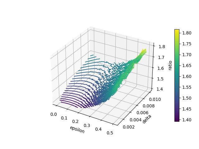
(a) ratio $n_{ho}/n_{wcc}$

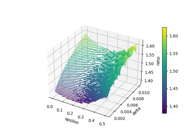
(b) ratio $n_{ho}/n_{cp}$

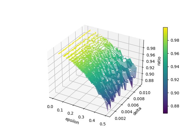
(c) ratio $n_{wcc}/n_{cp}$

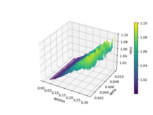
(d) ratio $n_{ho}/n_{cp}$ for $\hat{p}=\frac{1}{10}$

Figure 4: Ratio of sample complexity for different confidence thresholds $\delta$ and precisions $\varepsilon$ between Hoeffding bound ($n_{ho}$, and Wilson score with CC ($n_{wcc}$) and Clopper-Pearson interval ($n_{cp}$), respectively

In Sec. 3.3 we discuss the ratio between sample complexities for the Hoeffding bound and the Wilson score with CC, or Clopper-Pearson interval, respectively. For an empirical approach, Fig. 2 plots these ratios for a range of different precisions $\varepsilon$ and two selected confidence thresholds $\delta$. From a theoretical perspective, we prove in Lemma 2 that for the Wilson score this ratio converges to a value $\geq 1$ for a given $\delta$ and $\varepsilon\rightarrow 0$. Moreover, we established that again for $\varepsilon\rightarrow 0$ this ratio is larger for larger $\delta$. A question that remains is whether this positive correlation of the ratio with $\delta$ also holds for larger values of $\varepsilon$. While we cannot formally answer this question, we can address it empirically. In Fig. 4 we present the ratios between the sample complexity of the three methods.

First of all, Figs. 4(a) and 4(b) again show once again that the Hoeffding bound is always outperformed by the other two methods. We again see that the ratio between the sample complexity of the Hoeffding bound and any of the other two methods decreases with decreasing the precisoin $\varepsilon$, although we see in particular for the Clopper-Pearson bound that also value of $\varepsilon$ close to $0$ increase the ratio, although mostly only for larger $\delta$. In general, this also supports the conjecture that the ratio is positively correlated with $\delta$ as well. As a remark, this means it is even more valuable to increase the confidence budget using the structural improvement methods from Sec. 4.

Wilson Score With Continuity Correction Vs. Clopper-Pearson Interval.

While we have at various points established that the Hoeffding bound is inferior to the Wilson score with continuity correction and the Clopper-Pearson interval, we have not yet explicitly compared the latter two against each other. In Fig. 4(c) we compare the worst-case sample complexity of the two against each other, again for various confidence thresholds $\delta$ and precision parameters $\varepsilon$. For all parameters the Wilson score requires less samples than the Clopper-Pearson interval. Additionally, for larger $\varepsilon$, the difference becomes significantly larger, whereas for $\varepsilon$ close to $0$ both perform basically equivalently. We do not observe any correlation of the ratio with $\delta$.

Does this mean one should dismiss the Clopper-Pearson interval in favor of the Wilson score interval? Not quite. So far we have only considered the worst-case scenario of $\hat{p}=\frac{1}{2}$. While this is instrumental for analysing the worst-case complexity bound, in practice this may of course not always be the case. In Fig. 4(d) we again plot the ratio between the required amount of samples with the Wilson score and the Clopper-Pearson interval but this time assuming that $\hat{p}=\frac{1}{10}$. Indeed we can now see that here the Clopper-Pearson interval requires less samples than the Wilson score with CC. Interestingly, even the correlation with $\varepsilon$ is inverted compared to Fig. 4(c). Unchanged, we notice that for $\varepsilon$ close to $0$, again both require roughly equal amounts of samples.

To summarise, we recommend to not use the Hoeffding bound to build confidence intervals for binomial parameters. If the success rate of the sampling process is close to $0$ or $1$, the Clopper-Pearson interval tends to produce smaller confidence intervals, whereas for $\hat{p}$ closer to $\frac{1}{2}$, and therefore also for a worst-case sample complexity analysis, we would recommend using the Wilson score interval with continuity correction. That being said, in practice confidence width may not always be the optimal measure to optimise for, and the method should be chosen with respect to the context in which it is applied. For example in applications such as total reward properties, it may be more important to prove the probability of a self loop is far away from 0 than to minimise the size of the interval of possible probabilities.

Appendix 0.C Additional Details on the Evaluation

Table 3: Model-SMC improvement factor per problem instance and improvement

Model / Property Parameters Transitions Wil CP Support ISAP MEC Chains All Reach consensus.disagree 2-2 184 1.371 1.37 1.092 1.006 1 1.405 2.212 2.21 2-4 376 1.34 1.34 1.084 1.006 1 1.483 2.256 2.26 4-2 29376 1.231 1.23 1.055 1.004 1 1.008 1.329 1.67 4-4 57024 1.22 1.22 1.052 1.004 1 1.009 1.314 1.60 csma.all_before_max 2-2 308 1.348 1.348 1.006 1.006 1 2.014 2.778 56.25 2-4 2812 1.278 1.278 1.002 1.005 1 1.872 2.416 63.31 3-2 23250 1.235 1.234 1.001 1.004 1 1.07 1.329 2.23 firewire_dl.deadline 3-200 1872 1.289 1.288 1.071 1.005 1 1 1.41 100.8 3-400 6936 1.258 1.257 1.062 1.004 1 1 1.36 5.41 mer.k_equal_n 3 3584 1.273 1.272 1.066 1.005 1.431 1 1.999 5.09 4 29410 1.231 1.23 1.055 1.004 1.614 1 2.147 5.14 pacman.crash 10 557 1.326 1.325 1.047 1.006 1 1.84 2.543 1579 5 52 1.44 1.439 1.091 1.007 1 1.966 3.091 121.8 wlan.collisions_max 2 2656 1.28 1.279 1 1.005 1 1.013 1.305 3.911 3 3968 1.27 1.269 1 1.005 1 1.009 1.289 2.609 wlan_dl.deadline 0 84096 1.215 1.214 1 1.004 1 1 1.22 5.053 1 299024 1.198 1.198 1.021 1.003 1 1.019 1.23 15.64 zeroconf.correct_max 100-2-T 296 1.35 1.349 1.079 1.006 1 1.289 1.918 2.998 100-4-T 472 1.332 1.331 1.077 1.006 1 1.153 1.694 2.503 20-2-F 82940 1.215 1.214 1.049 1.004 1 1.001 1.286 2.985 20-2-T 296 1.35 1.349 1.079 1.006 1 1.289 1.918 2.998 20-4-T 472 1.332 1.331 1.077 1.006 1 1.153 1.694 2.503 zeroconf_dl.deadline_max 1000-1-F-10 10150 1.25 1.249 1.054 1.004 1 1.175 1.543 298.6 1000-1-F-20 47268 1.223 1.222 1.049 1.004 1 1.083 1.392 15.96 1000-1-T-10 2038 1.287 1.286 1.059 1.005 1 1.069 1.448 47.1 1000-1-T-20 3978 1.27 1.269 1.056 1.005 1 1.034 1.38 5.676

Table 4: Property-SMC results including parameters and runtimes

			Samples		runtime
Model / Property	Parameters	Precision	Base	Ours	Base	Ours	Factor
consensus.disagree	2-2	0.3382	5520	754	1.3	0.7	7
csma.all_before_max	2-2	0.1114	9240	637	2.7	0.4	15
firewire_dl.deadline	3-200	0.0751	56160	24732	39.8	0.9	2
mer.k_equal_n	3	0.5564	77400	41662	11.5	3.7	2
pacman.crash	5	0.1718	1560	99	0.5	0.4	16
wlan.collisions_max	2	0.7241	79680	5859	18.9	0.8	14
wlan_dl.deadline	0	0.9141	2483520	179046	2502	12.7	14
zeroconf.correct_max	20-2-T	0.0664	8880	112	1.0	0.4	79
zeroconf_dl.deadline_max	1000-1-T-10	0.0425	61140	455	3.7	0.5	134

Here, we show the full tables of Table 1 and Table 2 referenced in Sec. 5. The values of the parameters are in order as in the PRISM benchmark suite.

In Table 3 we show the improvement factor for each combination of problem instance and improvement. We see that both the Wilson score with CC and Clopper-Pearson interval provide is slightly negatively correlated with model size, matching our evaluation in Sec. 3.3, as a larger model corresponds a smaller error threshold per transition probability. As described in Sec. 5 the models from the PRISM benchmark suite do not contain any collapsable MECs, hence we observe an improvement factor of 1 for exactly these models. Similarly, for the two-successor improvement we obtain an improvement factor of 1 for models without binary branching state-action pairs, and for the contractions of chains we obtain an improvement factor of 1 for models without chains of course. In some cases, specifically certain variants of consensus, we see that instance-specific Model-SMC does not bring any advantage over standard Model-SMC using all improvements. This implies that for these instances all transitions are relevant to decide with what probability the objective holds in the initial state, and thus no further improvement can be made. We do however notice in our implementation that the model may still be smaller after applying the instance-specific improvements as MECs and states with labels not relevant to the objective may be combined into a single sink state.

In Table 4, we extend Table 2 by parameters and runtimes. For each model, we first collect a data set from sample runs, where each sample run is a path starting in the initial state and reaches either a goal state or a sink state under the scheduler that uniformly at random picks an action in each state. For the number of sample runs we choose 30 times the number of probabilistic transitions in the model (see column “Transitions” in Table 3). The reason for this is that we expect the number of samples required to determine the reachability objective up to a meaningful precision is proportional to the size of the model. This dataset is then used to calculate a $\delta=0.1$ confidence interval $[\underline{V}(\hat{s}),\overline{V}(\hat{s})]$ for the probability of reaching the goal from the initial state $\hat{s}$, using the baseline algorithm. In column “precision” we report the width $\varepsilon=\overline{V}(\hat{s})-\underline{V}(\hat{s})$ of the interval. We then run our improved algorithm with all improvement discussed in the paper while on incrementally larger subsets of the initial dataset. Naturally, we add paths in the order they were sampled. We do this until we are able to achieve a precision of at least $\varepsilon$ w.r.t the objective as well. Under “samples runs” in column “Ours” we then report how many paths are included in the smallest dataset fragment sufficient to obtain the given precision. Finally, in the columns “runtime” we give the runtime of both the baseline algorithm, and our improved algorithm in seconds. Note that for our algorithm we only report the time required to compute $\varepsilon$ with the dataset fragment sufficient to achieve a precision of $\varepsilon$, not the time required to find this dataset fragment.

As mentioned in Sec. 5, for a given instance of model and reachability objective, there is no clear correlation between the worst-case analysis in instance-specific Model-SMC (see column “Instance-specific” in Table 3) and Property-SMC (see column “Factor” Table 4). For example, while wlan only has improvement factors of around 4 in instance-specific Model-SMC, it has an improvement factor of over 13 in Property-SMC. On the other hand, firewire_dl, has a large improvement factor of over 100 in instance-specific Model-SMC, but only an improvement factor of 2.271 in Property-SMC. We identify three possible explanations for such deviations:

• Model-SMC performs a worst-case analysis. In particular it assumes a uniform distribution for each transition. This may of course not necessarily be the case in the actual models.

• Model-SMC assumes full sampling access whereas in our Property-SMC setting we only allow to sample runs from the initial state under a uniform strategy. Thus, for Property-SMC, it may happen that certain areas of the MDP receive less samples because they are hard to reach under a uniform strategy.

• Perhaps more importantly, Model-SMC does not pay attention to the structure of the MDP. However, knowing all transitions up to a certain precision does not translate to being able to determine a quantitative reachability up to a certain precision. One reason for this is that the probabilities in a path of an MDP propagate multiplicatively, thus putting an emphasis on the length of paths reaching the goal state which of course may differ between models.

In wlan the first explanation indeed applies, as most transitions in the model have uniform distributions over 16 successors, meaning it is unlikely we encounter the worst-case scenario of a successor being sampled for half the trials. This deviation from $\hat{p}=\frac{1}{2}$ does not impact the size of the Hoeffding interval since it is independent of $\hat{p}$, but it does have an effect on both the Wilson score with CC and Clopper-Pearson interval as we show in the proof of Lemma 1 That being said, we find that the other possible explanations are hard to verify since it is hard to measure them. Thus we cannot ultimately say that these are indeed the only driving factors behind this phenomenon.

The runtime improvement here scales with the number of states that can be collapsed in the instance-specific improvements. As noted before, this is not necessarily correlated with the impact of the instance-specific improvements on the sample requirements. This can be seen especially in the wlan example again where the instance-specific improvements did not remove any (probabilistic) transitions and thus did not impact the worst-case sample complexity. However, even just collapsing deterministic parts of the MDP into a single sink or goal state has a big impact on the runtime.

References

- [1] Alekh Agarwal, Sham M. Kakade, and Lin F. Yang. Model-based reinforcement learning with a generative model is minimax optimal. In COLT, volume 125 of Proceedings of Machine Learning Research, pages 67–83. PMLR, 2020.
- [2] Chaitanya Agarwal, Shibashis Guha, Jan Křetínskỳ, and Pazhamalai Muruganandham. Pac statistical model checking of mean payoff in discrete-and continuous-time mdp. In International Conference on Computer Aided Verification, pages 3–25. Springer, 2022.
- [3] Gul Agha and Karl Palmskog. A survey of statistical model checking. ACM Trans. Model. Comput. Simul., 28(1):6:1–6:39, 2018.
- [4] Alan Agresti and Brent A Coull. Approximate is better than “exact” for interval estimation of binomial proportions. The American Statistician, 52(2):119–126, 1998.
- [5] Murray Aitkin, Dorothy Anderson, Brian Francis, and John Hinde. Statistical modelling in glim. pages 112–118, 1988.
- [6] Mohammed Alshiekh, Roderick Bloem, Rüdiger Ehlers, Bettina Könighofer, Scott Niekum, and Ufuk Topcu. Safe reinforcement learning via shielding. In AAAI, pages 2669–2678. AAAI Press, 2018.
- [7] Pranav Ashok, Krishnendu Chatterjee, Przemyslaw Daca, Jan Kretínský, and Tobias Meggendorfer. Value iteration for long-run average reward in Markov decision processes. In CAV (1), volume 10426 of Lecture Notes in Computer Science, pages 201–221. Springer, 2017.
- [8] Pranav Ashok, J.an Kretínský, and Maximilian Weininger. PAC statistical model checking for markov decision processes and stochastic games. In CAV, Part I, volume 11561 of LNCS, pages 497–519. Springer, 2019.
- [9] Dimitris Askitis. Logarithmic concavity of the inverse incomplete beta function with respect to parameter. Mathematica Scandinavia, 127, 10 2017.
- [10] Peter Auer, Thomas Jaksch, and Ronald Ortner. Near-optimal regret bounds for reinforcement learning. Advances in neural information processing systems, 21, 2008.
- [11] Thom S. Badings, Licio Romao, Alessandro Abate, David Parker, Hasan A. Poonawala, Mariëlle Stoelinga, and Nils Jansen. Robust control for dynamical systems with non-gaussian noise via formal abstractions. J. Artif. Intell. Res., 76:341–391, 2023.
- [12] Thom S. Badings, Thiago D. Simão, Marnix Suilen, and Nils Jansen. Decision-making under uncertainty: beyond probabilities. Int. J. Softw. Tools Technol. Transf., 25(3):375–391, 2023.
- [13] Christel Baier, Clemens Dubslaff, Patrick Wienhöft, and Stefan J. Kiebel. Strategy synthesis in markov decision processes under limited sampling access. In Kristin Y. Rozier and Swarat Chaudhuri, editors, NASA Formal Methods, volume 13903 of Lecture Notes in Computer Science, page 86–103. Springer, 2023.
- [14] Christel Baier and Joost-Pieter Katoen. Principles of model checking. MIT Press, 2008.
- [15] Christel Baier, Joachim Klein, Linda Leuschner, David Parker, and Sascha Wunderlich. Ensuring the reliability of your model checker: Interval iteration for markov decision processes. In CAV (1), volume 10426 of Lecture Notes in Computer Science, pages 160–180. Springer, 2017.
- [16] Hugo Bazille, Blaise Genest, Cyrille Jégourel, and Jun Sun. Global PAC bounds for learning discrete time markov chains. In CAV (2), volume 12225 of Lecture Notes in Computer Science, pages 304–326. Springer, 2020.
- [17] George Bennett. Probability inequalities for the sum of independent random variables. Journal of the American Statistical Association, 57(297):33–45, 1962.
- [18] François Bergeron, Gilbert Labelle, and Pierre Leroux. Combinatorial Species and Tree-like Structures. Encyclopedia of Mathematics and its Applications. Cambridge University Press, 1997.
- [19] Sergei Bernstein. On a modification of chebyshev’s inequality and of the error formula of laplace. Ann. Sci. Inst. Sav. Ukraine, Sect. Math, 1(4):38–49, 1924.
- [20] Colin R Blyth and Harold A Still. Binomial confidence intervals. Journal of the American Statistical Association, 78(381):108–116, 1983.
- [21] Stéphane Boucheron, Gábor Lugosi, and Pascal Massart. Concentration Inequalities: A Nonasymptotic Theory of Independence. Oxford University Press, 2013.
- [22] T. Brázdil, K. Chatterjee, M. Chmelik, V. Forejt, J. Křetínský, M. Z. Kwiatkowska, D. Parker, and M. Ujma. Verification of Markov decision processes using learning algorithms. In ATVA, pages 98–114. Springer, 2014.
- [23] Lawrence D. Brown, T. Tony Cai, and Anirban DasGupta. Interval Estimation for a Binomial Proportion. Statistical Science, 16(2):101 – 133, 2001.
- [24] George Casella and Charles E McCulloch. Confidence intervals for discrete distributions. 1984.
- [25] Jianhua Chen. Properties of a new adaptive sampling method with applications to scalable learning. Web Intell., 13(4):215–227, 2015.
- [26] Charles J Clopper and Egon S Pearson. The use of confidence or fiducial limits illustrated in the case of the binomial. Biometrika, 26(4):404–413, 1934.
- [27] Costas Courcoubetis and Mihalis Yannakakis. The complexity of probabilistic verification. J. ACM, 42(4):857–907, 1995.
- [28] Przemyslaw Daca, Thomas A. Henzinger, Jan Kretínský, and Tatjana Petrov. Faster statistical model checking for unbounded temporal properties. ACM Trans. Comput. Log., 18(2):12:1–12:25, 2017.
- [29] Pedro R. D’Argenio, Arnd Hartmanns, and Sean Sedwards. Lightweight statistical model checking in nondeterministic continuous time. In ISoLA (2), volume 11245 of Lecture Notes in Computer Science, pages 336–353. Springer, 2018.
- [30] Pedro R. D’Argenio, Axel Legay, Sean Sedwards, and Louis-Marie Traonouez. Smart sampling for lightweight verification of markov decision processes. Int. J. Softw. Tools Technol. Transf., 17(4):469–484, 2015.
- [31] Luca De Alfaro. Formal verification of probabilistic systems. PhD thesis, Stanford university, 1997.
- [32] Diane E Duffy and Thomas J Santner. Confidence intervals for a binomial parameter based on multistage tests. Biometrics, pages 81–93, 1987.
- [33] Lu Feng, Marta Z. Kwiatkowska, and David Parker. Automated learning of probabilistic assumptions for compositional reasoning. In FASE, volume 6603 of Lecture Notes in Computer Science, pages 2–17. Springer, 2011.
- [34] Vojtech Forejt, Marta Z. Kwiatkowska, Gethin Norman, and David Parker. Automated verification techniques for probabilistic systems. In SFM, volume 6659 of Lecture Notes in Computer Science, pages 53–113. Springer, 2011.
- [35] Jie Fu and Ufuk Topcu. Probably approximately correct MDP learning and control with temporal logic constraints. In Robotics: Science and Systems, 2014.
- [36] Robert Givan, Sonia Leach, and Thomas Dean. Bounded-parameter markov decision processes. Artificial Intelligence, 122(1-2):71–109, 2000.
- [37] Serge Haddad and Benjamin Monmege. Interval iteration algorithm for MDPs and IMDPs. Theor. Comput. Sci., 735:111–131, 2018.
- [38] Ernst Moritz Hahn, Mateo Perez, Sven Schewe, Fabio Somenzi, Ashutosh Trivedi, and Dominik Wojtczak. Omega-regular objectives in model-free reinforcement learning. In TACAS (1), volume 11427 of Lecture Notes in Computer Science, pages 395–412. Springer, 2019.
- [39] Ernst Moritz Hahn, Mateo Perez, Sven Schewe, Fabio Somenzi, Ashutosh Trivedi, and Dominik Wojtczak. Mungojerrie: Linear-time objectives in model-free reinforcement learning. In TACAS (1), volume 13993 of Lecture Notes in Computer Science, pages 527–545. Springer, 2023.
- [40] Aria HasanzadeZonuzy, Archana Bura, Dileep M. Kalathil, and Srinivas Shakkottai. Learning with safety constraints: Sample complexity of reinforcement learning for constrained mdps. In AAAI, pages 7667–7674. AAAI Press, 2021.
- [41] Wassily Hoeffding. Probability inequalities for sums of bounded random variables. Journal of the American Statistical Association, 58(301):13–30, 1963.
- [42] Hui Jiang. Machine Learning Fundamentals. Cambridge University Press, 2021.
- [43] Chi Jin, Akshay Krishnamurthy, Max Simchowitz, and Tiancheng Yu. Reward-free exploration for reinforcement learning. In ICML, volume 119 of Proceedings of Machine Learning Research, pages 4870–4879. PMLR, 2020.
- [44] J. Kretínský, F. Michel, L. Michel, and G. A. Pérez. Finite-memory near-optimal learning for markov decision processes with long-run average reward. In UAI, volume 124 of Proceedings of Machine Learning Research, pages 1149–1158. AUAI Press, 2020.
- [45] Jan Kretínský. Survey of statistical verification of linear unbounded properties: Model checking and distances. In ISoLA (1), volume 9952 of Lecture Notes in Computer Science, pages 27–45, 2016.
- [46] Jan Křetínský, Guillermo A. Pérez, and Jean-François Raskin. Learning-based mean-payoff optimization in an unknown MDP under omega-regular constraints. In CONCUR, pages 8:1–8:18. Dagstuhl, 2018.
- [47] Marta Z. Kwiatkowska, Gethin Norman, and David Parker. The PRISM benchmark suite. In QEST, pages 203–204. IEEE Computer Society, 2012.
- [48] Sascha Lange, Thomas Gabel, and Martin A. Riedmiller. Batch reinforcement learning. In Reinforcement Learning, volume 12 of Adaptation, Learning, and Optimization, pages 45–73. Springer, 2012.
- [49] Axel Legay, Anna Lukina, Louis-Marie Traonouez, Junxing Yang, Scott A. Smolka, and Radu Grosu. Statistical model checking. In Computing and Software Science, volume 10000 of Lecture Notes in Computer Science, pages 478–504. Springer, 2019.
- [50] Axel Legay, Sean Sedwards, and Louis-Marie Traonouez. Scalable verification of markov decision processes. In SEFM Workshops, volume 8938 of Lecture Notes in Computer Science, pages 350–362. Springer, 2014.
- [51] Andreas Maurer and Massimiliano Pontil. Empirical bernstein bounds and sample variance penalization. arXiv preprint arXiv:0907.3740, 2009.
- [52] Tobias Meggendorfer. PET - A partial exploration tool for probabilistic verification. In Ahmed Bouajjani, Lukás Holík, and Zhilin Wu, editors, Automated Technology for Verification and Analysis - 20th International Symposium, ATVA 2022, Virtual Event, October 25-28, 2022, Proceedings, volume 13505 of Lecture Notes in Computer Science, pages 320–326. Springer, 2022.
- [53] Robert G Newcombe. Interval estimation for the difference between independent proportions: comparison of eleven methods. Statistics in medicine, 17(8):873–890, 1998.
- [54] Mateo Perez, Fabio Somenzi, and Ashutosh Trivedi. A PAC learning algorithm for LTL and omega-regular objectives in mdps. CoRR, abs/2310.12248, 2023.
- [55] M.L. Puterman. Markov decision processes: Discrete stochastic dynamic programming. John Wiley and Sons, 1994.
- [56] Licio Romao, Antonis Papachristodoulou, and Kostas Margellos. On the exact feasibility of convex scenario programs with discarded constraints. IEEE Transactions on Automatic Control, 68(4):1986–2001, 2023.
- [57] Laixi Shi, Gen Li, Yuting Wei, Yuxin Chen, and Yuejie Chi. Pessimistic q-learning for offline reinforcement learning: Towards optimal sample complexity. In ICML, volume 162 of Proceedings of Machine Learning Research, pages 19967–20025. PMLR, 2022.
- [58] Anthony J. Strecok. On the calculation of the inverse of the error function. Mathematics of Computation, 22(101):144–158, 1968.
- [59] Alexander L Strehl and Michael L Littman. An empirical evaluation of interval estimation for markov decision processes. In 16th IEEE International Conference on Tools with Artificial Intelligence, pages 128–135. IEEE, 2004.
- [60] Marnix Suilen, Thiago D. Simão, David Parker, and Nils Jansen. Robust anytime learning of markov decision processes. In NeurIPS, 2022.
- [61] Robert Endre Tarjan. Depth-first search and linear graph algorithms. SIAM J. Comput., 1(2):146–160, 1972.
- [62] Nico M Temme. Asymptotic inversion of the incomplete beta function. Journal of computational and applied mathematics, 41(1-2):145–157, 1992.
- [63] Andrew J. Wagenmaker, Max Simchowitz, and Kevin Jamieson. Beyond no regret: Instance-dependent PAC reinforcement learning. In COLT, volume 178 of Proceedings of Machine Learning Research, pages 358–418. PMLR, 2022.
- [64] Sean Wallis. Binomial confidence intervals and contingency tests: Mathematical fundamentals and the evaluation of alternative methods. J. Quant. Linguistics, 20(3):178–208, 2013.
- [65] Maximilian Weininger, Kush Grover, Shruti Misra, and Jan Kretínský. Guaranteed trade-offs in dynamic information flow tracking games. In CDC, pages 3786–3793. IEEE, 2021.
- [66] Tsachy Weissman, Erik Ordentlich, Gadiel Seroussi, Sergio Verdu, and Marcelo J Weinberger. Inequalities for the l1 deviation of the empirical distribution. Hewlett-Packard Labs, Tech. Rep, 2003.
- [67] Min Wen and Ufuk Topcu. Probably approximately correct learning in adversarial environments with temporal logic specifications. IEEE Trans. Autom. Control., 67(10):5055–5070, 2022.
- [68] Patrick Wienhöft, Marnix Suilen, Thiago D Simão, Clemens Dubslaff, Christel Baier, and Nils Jansen. More for less: Safe policy improvement with stronger performance guarantees. arXiv preprint arXiv:2305.07958, 2023.
- [69] Patrick Wienhöft, Marnix Suilen, Thiago D. Simão, Clemens Dubslaff, Christel Baier, and Nils Jansen. More for less: Safe policy improvement with stronger performance guarantees. In Proceedings of the International Joint Conference on Artificial Intelligence (IJCAI), 2023.
- [70] Edwin B Wilson. Probable inference, the law of succession, and statistical inference. Journal of the American Statistical Association, 22(158):209–212, 1927.
- [71] H. L. S. Younes and R. G. Simmons. Probabilistic verification of discrete event systems using acceptance sampling. In CAV, pages 223–235. Springer, 2002.