Joint Active and Passive Beamforming for IRS-Aided Wireless Energy Transfer Network Exploiting One-Bit Feedback

Abstract

To reap the active and passive beamforming gain in an intelligent reflecting surface (IRS)-aided wireless network, a typical way is to first acquire the channel state information (CSI) relying on the pilot signal, and then perform the joint beamforming design. However, it is a great challenge when the receiver can neither send pilot signals nor have complex signal processing capabilities due to its hardware limitation. To tackle this problem, we study in this paper an IRS-aided wireless energy transfer (WET) network and propose two joint beamforming design methods, namely, the channel-estimation-based method and the distributed-beamforming-based method, that require only one-bit feedback from the energy receiver (ER) to the energy transmitter (ET). Specifically, for the channel-estimation-based method, according to the feedback information, the ET is able to infer the cascaded ET-IRS-ER channel by continually adjusting its transmit beamformer while applying the analytic center cutting plane method (ACCPM). Then, based on the estimated cascaded CSI, the joint beamforming design can be performed by using the existing optimization techniques. While for the distributed-beamforming-based method, we first apply the distributed beamforming algorithm to optimize the IRS reflection coefficients, which is theoretically proven to converge to a local optimum almost surely. Then, the optimal ET’s transmit covariance matrix is obtained based on the effective ET-ER channel learned by applying the ACCPM only once. Numerical results demonstrate the effectiveness of our proposed one-bit-feedback-based joint beamforming design schemes while greatly reducing the requirement on the hardware complexity of the ER. In particular, the high accuracy of our IRS-involved cascaded channel estimation method exploiting one-bit feedback is also validated.

I Introduction

To achieve the vision that descripted as “global coverage, all spectra, full applications, all senses, all digital, and strong security” for the sixth-generation (6G) wireless communication systems [1], the traditional thinking that wireless communication technology needs to adapt to uncontrollable wireless channels should be broken. Intelligent reflecting surface (IRS), with the ability to smartly reshape the electromagnetic propagation environment in real time to enhance wireless system performance, has been proposed as a promising new paradigm for the future 6G wireless networks [2, 3, 4, 5, 6]. Typically, IRSs are implemented by a large number of low-cost passive elements (e.g., positive-intrinsic-negative (PIN) diodes, field-effect transistors (FETs), or micro-electromechanical system (MEMS) switches [5]), and do not rely on active hardware components such as radio frequency (RF) chains. By finely adjusting the phase shifts (PSs) of the passive IRS reflecting elements, the incident signals can be dynamically shaped to meet diverse system requirements, including the spectral and energy efficiency improvements [7, 8, 9, 10], communication coverage expansion [11, 12, 13], physical layer security enhancement [14, 15], etc. In general, the introduction of IRS brings about a new design degree of freedom (DoF) for improving the quality of channels to existing wireless systems without modifying the current physical layer standardization. Moreover, IRS has attractive characteristics such as low profile, light-weight, and conformal geometry, thus allowing its highly flexible deployment. All of the above significant advantages make IRS a promising research direction for both industry and academia.

Typically, to facilitate resource allocation and channel reconfiguration in an IRS-aided wireless network, a prerequisite is the acquisition of IRS-involved cascaded channel state information (CSI). Accordingly, the expected system performance gains brought by an IRS depend on accurate CSI estimation, which is a challenge since IRS is a passive component that can neither send nor receive pilot symbols, and its elements number is typically very large [16]. Take the downlink wireless transmission as an example, a widely adopted channel estimation approach is that for the systems operating in time-division duplex (TDD) protocol, the transmitter acquires the IRS-involved cascaded CSI by estimating the reverse link based on the training signals sent by the receiver [17, 18, 19]. However, this method critically depends on the degree of reciprocity between the forward and reverse links. Moreover, to improve the channel estimation accuracy, the receiver needs to send pilot symbols with sufficient power to effectively mitigate the impact of noise, which is unbearable for energy-constrained receiver, such as mobile phones in cellular network. Alternatively, another commonly adopted method to acquire the IRS-related cascaded CSI at the transmitter is to send the pilot signals from transmitter to receiver, through which the receiver can estimate the CSI and then send it back to the transmitter via a feedback channel [20, 21]. Although this method applies to both TDD and frequency-division duplex (FDD) adopted systems, it requires complex signal processing capabilities at the receiver for channel estimation, thus increasing its hardware cost. Responding to this, the beam training strategy is a desired method that facilitates both efficient channel estimation and beamforming design while reducing the hardware cost at the receiver [22, 23, 24]. However, it mainly takes advantage of the sparsity of millimeterwave (mmWave) or terahertz (THz) channels and can only realize the mainlobe alignment, thus it is not suitable for low-frequency wireless systems. The drawbacks of the existing channel estimation methods described above motivate us to investigate novel channel learning and beamforming approaches for IRS-aided wireless systems while taking the hardware limitation at the receiver into consideration in our work.

In this paper, we study an IRS-aided wireless energy transfer (WET) network, where an energy transmitter (ET) sends wireless energy to an energy receiver (ER) via transmit energy beamforming with the help of an IRS. It is assumed that the ER is unable to assist the ET to perform explicit channel estimation due to its hardware limitation, while it can periodically send one-bit feedback information, i.e., ‘0’ or ‘1’, to the ET over the dedicated feedback channel to help improve system performance. Based on this system setup, we propose two novel joint active ET and passive IRS beamforming design methods, namely, the channel-estimation-based method and the distributed-beamforming-based method, to boost the system performance.

For the channel-estimation-based method, we first estimate the cascaded ET-IRS-ER channel by continuously adjusting the transmit beamformer of the ET according to the feedback information from the ER each time. Each feedback bit indicates whether the energy harvested at the ER in the current interval is increasing or decreasing compared to the previous interval, which we assume can be accurately measured. It is worth noting that an optimization technique named analytic center cutting plane method (ACCPM) is applied during the channel learning phase. Then, in the following wireless energy transmission phase, based on the estimated channel, the transmit covariance matrix of the ET and the PSs of the IRS can be jointly optimized to maximize the amount of energy harvested at the ER by applying the existing optimization techniques. It should be mentioned that although the channel learning algorithms that require one-bit feedback were respectively proposed in [26] and [27], IRS was not applied in their studied systems, which as a passive component that greatly increases the difficulty of channel estimation.

For the distributed-beamforming-based method, we jointly optimize the ET’s transmit covariance matrix and the IRS reflection coefficients without explicitly estimating the cascaded ET-IRS-ER channel. Specifically, we first optimize the IRS reflection coefficients by applying the distributed beamforming algorithm, where each IRS element/group adjusts its PS value randomly at each iteration, and the ER gives one-bit of feedback indicating whether the amount of harvested energy is larger or smaller than that in previous iteration. If it is larger, all the IRS elements/groups will keep their latest PS perturbations; otherwise they all undo the PS perturbation. The above procedure is repeated until the convergence is reached. In addition, we theoretically show that for trivial perturbation distribution, with any given initial value, the PSs of IRS will converge to a local optimum with probability 1. Our feedback algorithm for optimizing the PSs of IRS elements can be seen as an extension of the distributed transmit beamforming algorithm proposed in [28] since the optimization variables are coupled in the objective function, which makes the proof of convergence more difficult. Then, based on the optimized IRS reflection coefficients, the effective ET-ER channel can be asymptotically obtained by using the ACCPM, and the optimal ET’s transmit covariance matrix can be therewith derived in closed form solution. It is worth noting that the above joint active and passive beamforming optimization procedures only need to be iterated once.

Finally, we perform extensive simulations to demonstrate the effectiveness of our proposed one-bit-feedback-based joint beamforming design methods, which significantly reduce the requirement for the hardware complexity of the ER simultaneously. In particular, it is also shown that our proposed channel-estimation-based method is able to estimate the cascaded ET-IRS-ER channel with high precision.

The rest of this paper is organized as follows. Section II introduces the system model and the problem formulation for joint active and passive beamforming design in IRS-aided WET network. In Section III and IV, we propose two efficient joint beamforming design methods, namely, the channel-estimation-based method and the distributed-beamforming-based method, based on one-bit feedback. Section V presents numerical results to evaluate the performance of the proposed joint beamforming design schemes. Finally, Section VI concludes the paper.

Notations: $\bf{I}$, $\bf{0}$, and $\bf{1}$ denote an identity matrix, an all-zero matrix, and an all-one matrix, respectively. $\mathbb{C}^{x\times y}$ denotes the space of $x\times y$ complex-valued matrices. For a complex number $x$, $\Re\left\{x\right\}$, $\Im\left\{x\right\}$, $\left|x\right|$, $\arg\left(x\right)$ denote its real part, imaginary part, modulus, and phase, respectively. For a complex-valued vector $\bf{x}$, $\left\|{\bf{x}}\right\|$ denotes its Euclidean norm. For any general matrix $\bf{X}$, ${\left\|{\bf{X}}\right\|_{F}}$, ${{\bf{X}}^{H}}$, ${\rm{rank}}\left({\bf{X}}\right)$, and ${\bf{X}}\left({i,j}\right)$ denote its Frobenius norm, conjugate transpose, rank, and $\left({i,j}\right)$th element, respectively. For a square matrix $\bf{A}$, $\det\left({\bf{A}}\right)$, ${\rm{tr}}\left({\bf{A}}\right)$ and ${{\bf{A}}^{-1}}$ denote its determinant, trace, and inverse, respectively, and ${\bf{A}}\succeq{\bf{0}}$ means that $\bf{A}$ is positive semi-definite. ${\rm{diag}}\left\{{{a_{1}},\cdots,{a_{n}}}\right\}$ denotes a square diagonal matrix with ${{a_{1}},\cdots,{a_{n}}}$ on the diagonal. $\mathbb{E}\left\{\cdot\right\}$ and $\Pr\left(\cdot\right)$ denote the statistical expectation and probability function, respectively. The Kronecker product and Khatri-Rao product are denoted by $\otimes$ and $\odot$, respectively. The distribution of a circularly symmetric complex Gaussian (CSCG) random vector with mean vector $\bf{x}$ and covariance matrix ${\bf{\Sigma}}$ is denoted by ${\cal C}{\cal N}\left({{\bf{x}},{\bf{\Sigma}}}\right)$, and $\sim$ stands for “distributed as”.

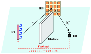
Figure 1: An indoor IRS-aided WET system where the ER feeds back one-bit of information to the ET periodically to assist the joint beamforming design for the system.

II System Model And Problem Formulation

As shown in Fig. 1, we consider a typical indoor IRS-assisted WET network, where an IRS consisting of $N$ passive reflecting elements is deployed to assist in the WET from an ET equipped with $M_{t}\geq 1$ antennas to a single-antenna ER. In particular, we consider a special case where the direct ET-to-ER transmission is blocked due to the unfavorable propagation conditions. Due to the hardware limitation at the ER, it can neither send pilot symbols nor perform complex signal processing operations, which makes the studied system fail to complete explicit channel estimation. However, the ER can periodically feed back one-bit of information to the ET based on the communication protocol to help the system improve its WET efficiency. The baseband equivalent channels from the ET to the IRS, from the IRS to the ER are denoted by ${\bf{G}}\in{\mathbb{C}^{N\times{M_{t}}}}$ and ${\bf{h}}_{r}^{H}\in{\mathbb{C}^{1\times N}}$, respectively. Since the ET, IRS, and ER are all placed in fixed positions, we assume that both the ET-IRS channel, $\bf{G}$, and the IRS-ER channel, ${\bf{h}}_{r}^{H}$, are quasi-static. Denote the duration of each channel coherence interval (CCI) as $T_{c}$, it is assumed to be sufficiently long for our proposed joint active and passive beamforming design schemes exploiting only one-bit feedback. We also assume that the ET can send $N_{d}\leq M_{t}$ energy beams, where the value of $N_{d}$ can be changed as needed. The $m$th beamforming vector and its corresponding energy-carried signal are denoted by ${{\bf{w}}_{m}}\in{\mathbb{C}^{{M_{t}}\times 1}}$ and ${s_{m}}\in\mathbb{C}$, respectively, with $m\in{{\cal N}_{d}}$ and ${{\cal N}_{d}}\buildrel\Delta\over{=}\left\{{1,2,\cdots,{N_{d}}}\right\}$. $\left\{{{s_{m}}}\right\}_{m=1}^{{N_{d}}}$ can be assumed to be independent random variables from any arbitrary distribution with zero mean and unit variance, i.e., $\mathbb{E}\big{\{}{{{\left|{{s_{m}}}\right|}^{2}}}\big{\}}=1,\forall m\in{{\cal N}_{d}}$, due to the fact that they do not carry any information. Thus, the transmitted signal at the ET is give by ${\bf{x}}=\sum\nolimits_{m=1}^{{N_{d}}}{{{\bf{w}}_{m}}{s_{m}}}$. Denote the set of reflecting elements of the IRS as ${\cal N}\buildrel\Delta\over{=}\left\{{1,2,\cdots N}\right\}$. The IRS reflection coefficient matrix can be modeled as ${\bf{\Theta}}={\rm{diag}}\left\{{{e^{j{\theta_{1}}}},{e^{j{\theta_{2}}}},\cdots,{e^{j{\theta_{N}}}}}\right\}$, where ${\theta_{n}}\in\left[{0,2\pi}\right),\forall n\in{\cal N}$, represents the PS corresponding to the $n$th IRS reflecting element. Accordingly, the ER’s received signal at time $t$ is given by

$$y\left(t\right)={\bf{h}}_{r}^{H}{\bf{\Theta}}\left(t\right){\bf{Gx}}\left(t\right)+n\left(t\right),$$ (1)

where $n\left(t\right)\sim{\cal C}{\cal N}\left({0,\sigma_{n}^{2}}\right)$ denotes the additive white Gaussian noise received by the ER at time $t$. Let ${\bf{v}}={\left[{{v_{1}},{v_{2}},\cdots{v_{N}}}\right]^{H}}$, where ${v_{n}}={e^{j{\theta_{n}}}}$, thus we have the following unit-modulus constraints: $\left|{{\bf{v}}\left(n\right)}\right|=1,\forall n\in\mathcal{N}$. By applying the change of variables, we have

$$y\left(t\right) ={{\bf{v}}^{H}}\left(t\right){\rm{diag}}\left({{\bf{h}}_{r}^{H}}\right){\bf{Gx}}\left(t\right)+n\left(t\right)$$

$$={{\bf{v}}^{H}}\left(t\right){{\bf{H}}_{c}}{\bf{x}}\left(t\right)+n\left(t\right),$$ (2)

where ${{\bf{H}}_{c}}={\rm{diag}}\left({{\bf{h}}_{r}^{H}}\right){\bf{G}}\in{\mathbb{C}^{N\times{M_{t}}}}$ is defined as the cascaded ET-IRS-ER channel. The energy harvested from noise is assumed to be negligible, thus the amount of the energy harvested at the ER is given by

$${E_{h}}\left(t\right)=\eta{\rm{tr}}\left({{{\bf{v}}^{H}}\left(t\right){{\bf{H}}_{c}}{\bf{Q}}\left(t\right){\bf{H}}_{c}^{H}{\bf{v}}\left(t\right)}\right),$$ (3)

where ${\bf{Q}}=\mathbb{E}\big{\{}{{\bf{x}}{{\bf{x}}^{H}}}\big{\}}=\sum\nolimits_{m=1}^{{N_{d}}}{{{\bf{w}}_{m}}{\bf{w}}_{m}^{H}}\succeq{\bf{0}}$ is the transmit covariance matrix at the ET, and $0<\eta\leq 1$ represents the energy harvesting efficiency. Since the ET has a maximum transmit power budget denoted by $P_{b}$, then we have ${\rm{tr}}\left({\bf{Q}}\right)\leq{P_{b}}$. Our objective is to maximize the amount of energy harvested at the ER without explicitly knowing the cascaded ET-IRS-ER channel ${{\bf{H}}_{c}}$, by jointly optimizing the transmit covariance matrix ${\bf{Q}}$ at the ET and the PS vector $\bf{v}$ at the IRS, while subject to the total transmit power constraint at the ET. As a result, we can formulate the problem as

$$\mathop{\max}\limits_{{\bf{Q}},{\bf{v}}}\ \eta{\rm{tr}}\big{(}{{{\bf{v}}^{H}}{{\bf{H}}_{c}}{\bf{QH}}_{c}^{H}{\bf{v}}}\big{)}$$ (4a)

$${\rm{s}}{\rm{.t}}{\rm{.}} \left|{{\bf{v}}\left(n\right)}\right|=1,\forall n\in{\cal N},$$ (4b)

$${\rm{tr}}\left({\bf{Q}}\right)\leq{P_{b}},$$ (4c)

$${\bf{Q}}\succeq{\bf{0}}.$$ (4d)

The key challenge for solving problem (4) lies in that we cannot explicitly obtain the required cascaded ET-IRS-ER channel ${{{\bf{H}}_{c}}}$, and there is only periodic one-bit feedback from the ER to the ET to be utilized to help adjust $\bf{Q}$ and $\bf{v}$. To tackle this intractability, in the next two sections we propose two novel joint active and passive beamforming design methods, namely, the channel-estimation-based method and the distributed-beamforming-based method, for our studied IRS-aided WET system by exploiting the ER’s one-bit feedback.

III Channel-Estimation-Based Method

In this section, we propose a novel channel-estimation-based joint active and passive beamforming design scheme for the IRS-aided WET network exploiting only one-bit feedback from the ER to the ET. Specifically, we first estimate a scaled version of the cascaded ET-IRS-ER channel by continuously adjusting ${\bf{Q}}$ and ${\bf{v}}$ according to the periodic one-bit feedback information from the ER to ET. Then, the optimal ${\bf{Q}}$ and ${\bf{v}}$ can be obtained by applying the existing optimization methods based on the estimated channel.

III-A IRS Elements Grouping

It can be readily seen that the dimension of the cascaded channel ${{{\bf{H}}_{c}}}$ grows linearly with the number of IRS elements, $N$, which can be huge in practice. For this, we adopt an IRS elements grouping method to reduce the channel learning overhead. The IRS elements in the same group are assigned a common reflection coefficient. Denote by $J$ the number of groups, we have

$${{\bf{v}}^{H}}{{\bf{H}}_{c}}=\left({{{{\bf{\bar{v}}}}^{H}}\odot\left[{{{\bf{1}}_{1\times{K_{1}}}},{{\bf{1}}_{1\times{K_{2}}}},\cdots,{{\bf{1}}_{1\times{K_{J}}}}}\right]}\right){{\bf{H}}_{c}},$$ (5)

where $\odot$ stands for the Khatri-Rao product, ${\bf{\bar{v}}}={\left[{{{\bar{v}}_{1}},{{\bar{v}}_{2}},\cdots,{{\bar{v}}_{J}}}\right]^{T}}\in{\mathbb{C}^{J\times 1}}$ represents the IRS group reflection coefficients, with ${{\bar{v}}_{j}}$ denoting the common reflection coefficient for the $j$th group, and ${K_{j}},\forall j\in{\cal J}$, is the number of the IRS elements in the $j$th group, with ${\cal J}\buildrel\Delta\over{=}\left\{{1,2,\cdots,J}\right\}$. Obviously, we have $\sum\nolimits_{j=1}^{J}{{K_{j}}}=N$. In our work, we assume equal size (number of IRS elements) of each group, which is given by $K=N/J$. Therefore, we have

$${{\bf{v}}^{H}}{{\bf{H}}_{c}} =\left({{{{\bf{\bar{v}}}}^{H}}\otimes{{\bf{1}}_{1\times K}}}\right){{\bf{H}}_{c}}$$

$$=\sum\limits_{i=1}^{N}{{{\left({{{{\bf{\bar{v}}}}^{H}}\otimes{{\bf{1}}_{1\times K}}}\right)}_{i}}{\bf{h}}_{c,i}^{H}}$$

$$=\sum\limits_{i=1}^{J}{{\bf{\bar{v}}}_{i}^{*}\sum\limits_{j=1}^{K}{{\bf{h}}_{c,j+\left({i-1}\right)K}^{H}}}$$

$$={{{\bf{\bar{v}}}}^{H}}{{{\bf{\bar{H}}}}_{c}},$$ (6)

where ${{\bf{h}}_{c,i}^{H}}$ is the $i$th row of ${{\bf{H}}_{c}}$, and ${\bf{\bar{h}}}_{c,i}^{H}=\sum\nolimits_{j=1}^{K}{{\bf{h}}_{c,j+\left({i-1}\right)K}^{H}}$ is the $i$th row of the group composite channel matrix ${{{\bf{\bar{H}}}}_{c}}$, denoting the combined composite reflecting channel associated with the $i$th IRS group. Based on this IRS elements grouping method, problem (4) is transformed into

$$\mathop{\max}\limits_{{\bf{Q}},{\bf{\bar{v}}}} \ {\rm{}}{\rm{tr}}\left({{\bf{P}}\left({{\bf{\bar{v}}}}\right){\bf{Q}}}\right)$$ (7a)

$${\rm{s}}{\rm{.t}}{\rm{.}} \ \left|{{\bf{\bar{v}}}\left(n\right)}\right|=1,\forall n\in{\cal J},$$ (7b)

$$\ \text{(\ref{P1}c)},\text{(\ref{P1}d)},$$ (7c)

where we define ${\bf{P}}\left({{\bf{\bar{v}}}}\right)=\eta{\bf{\bar{H}}}_{c}^{H}{\bf{\bar{v}}}{{{\bf{\bar{v}}}}^{H}}{{{\bf{\bar{H}}}}_{c}}$.

III-B Estimation of Group Composite Channel Matrix ${{{\bf{\bar{H}}}}_{c}}$

The following discussion is based on the assumption that for any ${{\bf{\bar{v}}}}$, we can accurately estimate the scaled version of ${\bf{P}}\left({{\bf{\bar{v}}}}\right)$, which is denoted as ${\bf{\tilde{P}}}\left({{\bf{\bar{v}}}}\right)$. We will discuss it in detail in the next subsection. Since ${\rm{rank}}\big{(}{{\bf{\tilde{P}}}\left({{\bf{\bar{v}}}}\right)}\big{)}=1$, by performing the eigenvalue decomposition (EVD) of ${\bf{\tilde{P}}}\left({{\bf{\bar{v}}}}\right)$, we have ${\bf{\tilde{P}}}\left({{\bf{\bar{v}}}}\right)={\bf{\tilde{p}}}\left({{\bf{\bar{v}}}}\right){{{\bf{\tilde{p}}}}^{H}}\left({{\bf{\bar{v}}}}\right)$, where $\left\|{{\bf{\tilde{p}}}\left({{\bf{\bar{v}}}}\right)}\right\|=\sqrt{{\rm{tr}}\big{(}{{\bf{\tilde{P}}}\left({{\bf{\bar{v}}}}\right)}\big{)}}$. Accordingly, the following equation

$${\bf{\bar{H}}}_{c}^{H}{\bf{\bar{v}}}=\gamma{\bf{\tilde{p}}}\left({{\bf{\bar{v}}}}\right)$$ (8)

holds, where $\gamma$ is a complex scaling factor. Based on this, by generating $C$ different IRS group reflection patterns, we have

$${\bf{\bar{H}}}_{c}^{H}{\bf{\bar{V}}}={\bf{\Lambda}}{\bf{R}},$$ (9)

where ${\bf{\bar{V}}}=\left[{{{{\bf{\bar{v}}}}_{1}},{{{\bf{\bar{v}}}}_{2}},\cdots,{{{\bf{\bar{v}}}}_{C}}}\right]\in{\mathbb{C}^{J\times C}}$, ${\bf{\Lambda}}=\left[{{\bf{\tilde{p}}}\left({{{{\bf{\bar{v}}}}_{1}}}\right),{\bf{\tilde{p}}}\left({{{{\bf{\bar{v}}}}_{2}}}\right),\cdots,{\bf{\tilde{p}}}\left({{{{\bf{\bar{v}}}}_{C}}}\right)}\right]\in{\mathbb{C}^{{M_{t}}\times C}}$, and ${\bf{R}}={\rm{diag}}\left\{{{\gamma_{1}},{\gamma_{2}},\cdots,{\gamma_{C}}}\right\}$. By applying the least squares (LS) estimator [30], the estimated ${\bf{\bar{H}}}_{c}^{H,{\rm{LS}}}$ is given by

$${\bf{\bar{H}}}_{c}^{H,{\rm{LS}}}={\bf{\Lambda}}{\bf{R}}{{{\bf{\bar{V}}}}^{\dagger}},$$ (10)

where ${{{\bf{\bar{V}}}}^{\dagger}}={{{\bf{\bar{V}}}}^{H}}{\left({{\bf{\bar{V}}}{{{\bf{\bar{V}}}}^{H}}}\right)^{-1}}$ is the pseudoinverse of ${{\bf{\bar{V}}}}$. It can be readily seen that $C$ should satisfy $C\geq J$. Therefore, to estimate the group composite channel ${{{\bf{\bar{H}}}}_{c}}$, the key is to obtain the accurate estimate of the scaled version of $\left\{{{\bf{P}}\left({{{{\bf{\bar{v}}}}_{i}}}\right)}\right\}_{i=1}^{C}$, i.e., $\big{\{}{{\bf{\tilde{P}}}\left({{{{\bf{\bar{v}}}}_{i}}}\right)}\big{\}}_{i=1}^{C}$, and determine the values of $\left\{{{\gamma_{i}}}\right\}_{i=1}^{C}$. In the next two subsections, we present the scaled channel learning approach and the scaling factor determination method, respectively.

III-C Scaled Channel Learning Using ACCPM

In this subsection, with the given ${{\bf{\bar{v}}}}$, we estimate the scaled version of ${{\bf{P}}\left({{\bf{\bar{v}}}}\right)}$, i.e., ${\bf{\tilde{P}}}\left({{\bf{\bar{v}}}}\right)$, based on the ER’s one-bit feedback by applying the ACCPM [26, 27]. ACCPM is an efficient localization method to solve general convex or quasi-convex optimization problems, with the goal of finding a feasible point in a convex target set. Specifically, at each iteration, the algorithm computes an analytic center of the current working set defined by the cutting-planes generated in previous iterations. If the calculated analytic center is a solution, then the algorithm will terminate; otherwise a new cutting plane returned by the oracle will be added into the current working set, thus forming a new working set for the next iteration. As the number of iterations increases, the working set gradually shrinks, and the algorithm will eventually find a solution to the problem.

Recall that we only need to obtain an estimate of the scaled ${\bf{P}}\left({{\bf{\bar{v}}}}\right)$. For simplicity, we define the target set as

$$\chi\buildrel\Delta\over{=}\big{\{}{{\bf{\tilde{P}}}\left({{\bf{\bar{v}}}}\right)|{\bf{0}}\preceq{\bf{\tilde{P}}}\left({{\bf{\bar{v}}}}\right)\preceq{\bf{I}},{\bf{\tilde{P}}}\left({{\bf{\bar{v}}}}\right)=\beta{\bf{P}}\left({{\bf{\bar{v}}}}\right),\forall\beta>0}\big{\}},$$ (11)

which contains all scaled matrices of ${{\bf{P}}\left({{\bf{\bar{v}}}}\right)}$ that satisfy ${\bf{0}}\preceq\beta{\bf{P}}\left({{\bf{\bar{v}}}}\right)\preceq{\bf{I}}$. Accordingly, the initial convex working set can be defined as ${{\cal P}_{0}}\buildrel\Delta\over{=}\big{\{}{{\bf{\tilde{P}}}\left({{\bf{\bar{v}}}}\right)|{\bf{0}}\preceq{\bf{\tilde{P}}}\left({{\bf{\bar{v}}}}\right)\preceq{\bf{I}}}\big{\}}$. Obviously, we have $\chi\subseteq{{\cal P}_{0}}$. In the following, we find a point in $\chi$ from ${\cal P}{{}_{0}}$ by applying the ACCPM.

Denote the transmit covariance matrix at the ET in interval $n,\forall n\in\mathbb{N}$, as ${{\bf{Q}}_{n}}$. Then, the energy harvested at the ER over the $n$th interval is given by

$${E_{h,n}}={T_{s}}{\rm{tr}}\left({{\bf{P}}\left({{\bf{\bar{v}}}}\right){{\bf{Q}}_{n}}}\right),$$ (12)

where $T_{s}$ is the duration of each interval. At the end of the interval $n$, the ER measures the amount of its harvested energy $E_{h,n}$, and feeds back one-bit information, denoted by ${{\tilde{f}}_{n}}\in\left\{{0,1}\right\}$, to indicate whether it is larger (${{\tilde{f}}_{n}}$ is set to ‘0’) or smaller (${{\tilde{f}}_{n}}$ is set to ‘1’) than that over the $\left(n-1\right)$th interval. To facilitate our analysis, we set ${f_{n}}=2{{\tilde{f}}_{n}}-1$ such that ${f_{n}}\in\left\{{-1,1}\right\}$. More concretely, we have ${f_{n}}=-1$ if ${E_{h,n}}\geq{E_{h,n-1}}$; or ${f_{n}}=1$ otherwise. For the sake of completeness, we define ${{\bf{Q}}_{0}}={\bf{0}}$, such that ${E_{h,0}}=0$. In this paper, we assume that $\left\{{{E_{h,n}}}\right\}$ are all perfectly measured at the ER. Therefore, each time the ET receives the one-bit feedback ${f_{n}}$ from the ER, it can obtain the following inequality:

$${f_{n}}{\rm{tr}}\left({{\bf{P}}\left({{\bf{\bar{v}}}}\right)\left({{{\bf{Q}}_{n}}-{{\bf{Q}}_{n-1}}}\right)}\right)\leq 0,\forall n\in\mathbb{N},$$ (13)

which means that ${{\bf{\tilde{P}}}\left({{\bf{\bar{v}}}}\right)}$ lies in the following half space:

$${{\cal H}_{n}}\buildrel\Delta\over{=}\left\{{{\bf{S}}|{f_{n}}{\rm{tr}}\left({{\bf{S}}\left({{{\bf{Q}}_{n}}-{{\bf{Q}}_{n-1}}}\right)}\right)\leq 0}\right\}.$$ (14)

Accordingly, compared to the working set at interval $n-1$, i.e., ${\cal P}{{}_{n-1}}$, the working set at interval $n\left(n\geq 2\right)$ is reduced to

$${{\cal P}_{n}} ={{\cal P}_{n-1}}\cap{{\cal H}_{n}}$$

$$=\big{\{}{{\bf{\tilde{P}}}\left({{\bf{\bar{v}}}}\right)|{\bf{0}}\preceq{\bf{\tilde{P}}}\left({{\bf{\bar{v}}}}\right)\preceq{\bf{I}},}\big{.}$$

$$\qquad\quad\big{.}{{f_{i}}{\rm{tr}}\big{(}{{\bf{\tilde{P}}}\left({{\bf{\bar{v}}}}\right)\left({{{\bf{Q}}_{i}}-{{\bf{Q}}_{i-1}}}\right)}\big{)}\leq 0,2\leq i\leq n}\big{\}}.$$ (15)

In particular, for $n=1$, we set ${{\cal P}_{1}}={{\cal P}_{0}}$. After ER’s $N_{f}$ feedbacks, we have

$${{\cal P}_{0}}={{\cal P}_{1}}\supseteq{{\cal P}_{2}}\supseteq\cdots\supseteq{{\cal P}_{{N_{f}}}}\supseteq\chi,$$ (16)

i.e., as the number of ER’s feedbacks increases, the working set ${{\cal P}_{n}}$ gradually shrinks to $\chi$. In Fig. 2, we illustrate the procedures of locating ${\cal P}{{}_{2}}$ in ${\cal P}{{}_{1}}$ and locating ${\cal P}{{}_{3}}$ in ${\cal P}{{}_{2}}$.

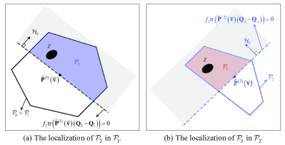
Figure 2: The procedure of ACCPM: the working set gradually shrinks to the target set.

Based on the principle of ACCPM, we need to query the oracle at the analytic center of the current working set ${{\cal P}_{n}}$ for localizing the next working set ${{\cal P}_{n+1}}$. The analytic center of ${{\cal P}_{n}}$ is explicitly given by [31]

$${{{\bf{\tilde{P}}}}^{\left(n\right)}}\left({{\bf{\bar{v}}}}\right) =\arg{\rm{}}\mathop{{\rm{min}}}\limits_{{\bf{0}}\preceq{\bf{\tilde{P}}}\preceq{\bf{I}}}{\rm{}}-2\log{\rm{det}}\big{(}{{\bf{\tilde{P}}}}\big{)}-2\log{\rm{det}}\big{(}{{\bf{I}}-{\bf{\tilde{P}}}}\big{)}$$

$$-\sum\limits_{i=2}^{n}{\log\big{(}{-{f_{i}}{\rm{tr}}\big{(}{{\bf{\tilde{P}}}\left({{{\bf{Q}}_{i}}-{{\bf{Q}}_{i-1}}}\right)}\big{)}}\big{)}},n\geq 0.$$ (17)

Although the problem in (III-C) is convex, its form does not support its direct solution with standard convex optimization solvers. For this reason, we rewrite the last term of (III-C) in a more compact form as follows. Define ${{{\bf{\bar{Q}}}}_{i}}=-{f_{i}}\left({{{\bf{Q}}_{i}}-{{\bf{Q}}_{i-1}}}\right)$ and ${\bf{\tilde{Q}}}=\left[{{{{\bf{\bar{Q}}}}_{2}},\cdots,{{{\bf{\bar{Q}}}}_{n}}}\right]$, we have

$$\sum\limits_{i=2}^{n}{\log\big{(}{-{f_{i}}{\rm{tr}}\big{(}{{\bf{\tilde{P}}}\left({{{\bf{Q}}_{i}}-{{\bf{Q}}_{i-1}}}\right)}\big{)}}\big{)}}$$

$$={\bf{1}}_{n-1}^{T}\log\big{(}{\left({{{\bf{I}}_{n-1}}\otimes{\bf{1}}_{{M_{t}}}^{T}}\right){\rm{diag}}\big{(}{\left({{{\bf{1}}_{n-1}}\otimes{{\bf{I}}_{{M_{t}}}}}\right){\bf{\tilde{P}\tilde{Q}}}}\big{)}}\big{)}.$$ (18)

Combined with (III-C), problem (III-C) can be efficiently solved by using standard convex optimization solvers such as CVX.

To efficiently implement the localization of $\chi$, with the given analytic center ${{{\bf{\tilde{P}}}}^{\left({n-1}\right)}}\left({{\bf{\bar{v}}}}\right)$ and the ET’s transmit covariance matrix ${{{\bf{Q}}_{n-1}}}$ at interval $n-1$, we need to guarantee that the resulting cutting plane is at least neutral, i.e., the cutting plane passes through the current analytic center. This guarantees a minimum worst-case total iteration number. Accordingly, the ET’s transmit covariance matrix at interval $n$, i.e., ${{\bf{Q}}_{n}}$, is constructed to satisfy

$${\rm{tr}}\big{(}{{{{\bf{\tilde{P}}}}^{\left(n-1\right)}}\left({{\bf{\bar{v}}}}\right)\left({{{\bf{Q}}_{n}}-{{\bf{Q}}_{n-1}}}\right)}\big{)}=0,\forall n\geq 2.$$ (19)

By this way, with the initial ET’s transmit covariance matrix for $n=1$ set to ${{\bf{Q}}_{1}}=\frac{{{P_{b}}}}{{{M_{t}}}}{{\bf{I}}_{{M_{t}}}}$, ${\left\{{{{\bf{Q}}_{n}}}\right\}_{n\geq 2}}$ can be obtained sequentially. Please refer to [26] for details.

III-D Determination of Scale Factor $\left\{{{\gamma_{i}}}\right\}$

We set the number of different IRS group reflection patterns to $C=J$, and design the IRS group reflection coefficient matrix ${{\bf{\bar{V}}}}$ as the Hadamard matrix of order $J$. Thus ${{{\bf{\bar{v}}}}_{j}},\forall j\in{\cal J}$, is the $j$th column of the $J$-order Hadamard matrix. Since a Hadamard matrix of order $2$ or $4$$k$ exists for every positive integer $k$, we assume that $J$ is a multiple of $4$ without loss of generality. Thanks to the IRS elements grouping method, the number of groups can be appropriately adjusted to make it feasible. From (10), we have

$${\bf{\bar{H}}}_{c}^{H,{\rm{LS}}} ={\bf{\Lambda R}}{{{\bf{\bar{V}}}}^{\dagger}}$$

$$={\bf{\Lambda R}}{{{\bf{\bar{V}}}}^{T}}{\left({{\bf{\bar{V}}}{{{\bf{\bar{V}}}}^{T}}}\right)^{-1}}$$

$$\mathop{=}\limits^{\left(a\right)}\frac{1}{J}{\bf{\Lambda R}}{{{\bf{\bar{V}}}}^{T}}$$

$$=\frac{1}{J}\sum\limits_{i=1}^{J}{{\gamma_{i}}{\bf{\tilde{p}}}\left({{{{\bf{\bar{v}}}}_{i}}}\right){\bf{\bar{v}}}_{i}^{T}},$$ (20)

where $\left(a\right)$ holds due to the property of Hadamard matrix. To perform joint active and passive beamforming design for the studied system, we only need to learn the scaled version of the cascaded channel ${\bf{\bar{H}}}_{c}$. Therefore, we just need to determine the ratio between any two from $\left\{{{\gamma_{i}}}\right\}_{i=1}^{J}$, including the amplitude ratio $\left|{{\gamma_{i}}}\right|/\left|{{\gamma_{j}}}\right|$ and phase difference $\angle{\gamma_{i}}-\angle{\gamma_{j}},\forall i\neq j$, and need not to know the true values of them. In the following, we convert the joint two-dimensional search for amplitude ratio and phase difference value into two separate one-dimensional searches. The details are given as follows.

III-D1 Amplitude Ratio Determination

From (8), with the given IRS group reflection coefficients ${{\bf{\bar{v}}}}$, the effective ET-ER channel can be expressed as

$${\bf{\tilde{h}}}_{r}^{H}={{{\bf{\bar{v}}}}^{H}}{{{\bf{\bar{H}}}}_{c}}={\gamma^{*}}{{{\bf{\tilde{p}}}}^{H}}\left({{\bf{\bar{v}}}}\right).$$ (21)

By adopting the maximum ratio transmission (MRT) precoding scheme with the transmit power set to $P_{t}$ at the ET, i.e., ${\bf{x}}=\sqrt{{P_{t}}}\frac{{{\bf{\tilde{p}}}\left({{\bf{\bar{v}}}}\right)}}{{\left\|{{\bf{\tilde{p}}}\left({{\bf{\bar{v}}}}\right)}\right\|}}$, the energy harvested at the ER over an interval is given by

$${E_{h}}\left({{P_{t}},{\bf{\bar{v}}}}\right)=\eta{T_{s}}{P_{t}}{\left|\gamma\right|^{2}}{\left\|{{\bf{\tilde{p}}}\left({{\bf{\bar{v}}}}\right)}\right\|^{2}}.$$ (22)

For any $i\neq j$, we can always find ${\bar{P}_{t,i}}$ and ${\bar{P}_{t,j}}$ such that ${E_{h,i}}\left({{{{\bar{P}}_{t,i}}},{{{\bf{\bar{v}}}}_{i}}}\right)={E_{h,j}}\left({{{{\bar{P}}_{t,j}}},{{{\bf{\bar{v}}}}_{j}}}\right)$ based on the ER’s one-bit feedback by applying the one-dimensional search in the power dimension. Then, the amplitude ratio can be calculated as

$$\frac{{\left|{{\gamma_{i}}}\right|}}{{\left|{{\gamma_{j}}}\right|}}=\sqrt{\frac{{{{{\bar{P}}_{t,j}}}}}{{{{{\bar{P}}_{t,i}}}}}}\frac{{\left\|{{\bf{\tilde{p}}}\left({{{{\bf{\bar{v}}}}_{j}}}\right)}\right\|}}{{\left\|{{\bf{\tilde{p}}}\left({{{{\bf{\bar{v}}}}_{i}}}\right)}\right\|}},\forall i\neq j.$$ (23)

The procedures for finding ${\bar{P}_{t,i}}$ and ${\bar{P}_{t,j}}$ to satisfy ${E_{h,i}}\left({{{{\bar{P}}_{t,i}}},{{{\bf{\bar{v}}}}_{i}}}\right)={E_{h,j}}\left({{{{\bar{P}}_{t,j}}},{{{\bf{\bar{v}}}}_{j}}}\right)$ are given as follows. Denote by the system configuration $\left\{{{P_{t}},{\bf{\bar{v}}}}\right\}$ as that the precoding vector ${\bf{x}}=\sqrt{{P_{t}}}\frac{{{\bf{\tilde{p}}}\left({{\bf{\bar{v}}}}\right)}}{{\left\|{{\bf{\tilde{p}}}\left({{\bf{\bar{v}}}}\right)}\right\|}}$ is adopted at the ET, and the group reflection coefficients ${{\bf{\bar{v}}}}$ is set at the IRS. In the first two timeslots, the system is configured with $\left\{{{P_{b}},{{{\bf{\bar{v}}}}_{i}}}\right\}$ and $\left\{{{P_{b}},{{{\bf{\bar{v}}}}_{j}}}\right\}$, respectively. Without loss of generality, we assume that ${E_{h}}\left({{{P_{b}},{{{\bf{\bar{v}}}}_{i}}}}\right)>{E_{h}}\left({{{P_{b}},{{{\bf{\bar{v}}}}_{j}}}}\right)$. Then, in the subsequent timeslots, we fix ${P_{t,j}}={P_{b}}$, and use the bisection method to search for ${{P_{t,i}}}$. By alternately configuring $\left\{{{P_{t,i}},{{{\bf{\bar{v}}}}_{i}}}\right\}$ and $\left\{{{P_{b}},{{{\bf{\bar{v}}}}_{j}}}\right\}$, the ${{{\bar{P}}_{t,i}}}$ can be eventually obtained such that ${E_{h,i}}\big{(}{{{\bar{P}}_{t,i}},{{{\bf{\bar{v}}}}_{i}}}\big{)}={E_{h,j}}\left({{P_{b}},{{{\bf{\bar{v}}}}_{j}}}\right)$.

III-D2 Phase Difference Determination

Prior to proceeding it, for any $i\neq j$, we multiply the vector ${\bf{\tilde{p}}}\left({{{{\bf{\bar{v}}}}_{j}}}\right)$ by a phase factor $e^{j{\varpi_{j}}}$, i.e., ${\bf{\tilde{p}}}\left({{{{\bf{\bar{v}}}}_{j}}}\right)\leftarrow{e^{j{\varpi_{j}}}}{\bf{\tilde{p}}}\left({{{{\bf{\bar{v}}}}_{j}}}\right)$, such that $\Im\left\{{{{{\bf{\tilde{p}}}}^{H}}\left({{{{\bf{\bar{v}}}}_{i}}}\right){\bf{\tilde{p}}}\left({{{{\bf{\bar{v}}}}_{j}}}\right)}\right\}=0$. Then, by setting the IRS group reflection coefficients as

$${\bf{\bar{v}}}_{i,j}^{c}=\frac{1}{2}\left({{{{\bf{\bar{v}}}}_{i}}+{{{\bf{\bar{v}}}}_{j}}}\right),$$ (24)

we have

$${\bf{\tilde{h}}}_{r}^{H}\left({{\bf{\bar{v}}}_{i,j}^{c}}\right)={\bf{\bar{v}}}_{i,j}^{c,T}{\bf{\bar{H}}}_{c}^{{\rm{LS}}}$$

$$=\frac{1}{{2J}}\left({{\bf{\bar{v}}}_{i}^{T}+{\bf{\bar{v}}}_{j}^{T}}\right)\sum\limits_{m=1}^{J}{\gamma_{m}^{*}{{{\bf{\bar{v}}}}_{m}}{{{\bf{\tilde{p}}}}^{H}}\left({{{{\bf{\bar{v}}}}_{m}}}\right)}$$

$$=\frac{1}{2}\left({\gamma_{i}^{*}{{{\bf{\tilde{p}}}}^{H}}\left({{{{\bf{\bar{v}}}}_{i}}}\right)+\gamma_{j}^{*}{{{\bf{\tilde{p}}}}^{H}}\left({{{{\bf{\bar{v}}}}_{j}}}\right)}\right)$$

$$=\frac{1}{2}\left|{{\gamma_{j}}}\right|{e^{-j\angle{\gamma_{j}}}}\big{(}{\frac{{\left|{{\gamma_{i}}}\right|}}{{\left|{{\gamma_{j}}}\right|}}{e^{-j\left({\angle{\gamma_{i}}-\angle{\gamma_{j}}}\right)}}{{{\bf{\tilde{p}}}}^{H}}\left({{{{\bf{\bar{v}}}}_{i}}}\right)+{{{\bf{\tilde{p}}}}^{H}}\left({{{{\bf{\bar{v}}}}_{j}}}\right)}\big{)}.$$ (25)

The following proposition shows that the phase difference $\angle{\gamma_{i}}-\angle{\gamma_{j}}$ can be determined by applying the one-dimensional search method.

Proposition 1

Let the transmit beamforming vector be

$${{\bf{x}}_{i,j}}\left(\vartheta\right)=\sqrt{{P_{b}}}\frac{{\left|{{\gamma_{i}}}\right|/\left|{{\gamma_{j}}}\right|{e^{j\vartheta}}{\bf{\tilde{p}}}\left({{{{\bf{\bar{v}}}}_{i}}}\right)+{\bf{\tilde{p}}}\left({{{{\bf{\bar{v}}}}_{j}}}\right)}}{{\left\|{\left|{{\gamma_{i}}}\right|/\left|{{\gamma_{j}}}\right|{e^{j\vartheta}}{\bf{\tilde{p}}}\left({{{{\bf{\bar{v}}}}_{i}}}\right)+{\bf{\tilde{p}}}\left({{{{\bf{\bar{v}}}}_{j}}}\right)}\right\|}}.$$ (26)

Then, the value of $\angle{\gamma_{i}}-\angle{\gamma_{j}}$ can be found by

$$\angle{\gamma_{i}}-\angle{\gamma_{j}}=\arg\mathop{{\rm{ext}}}\limits_{\vartheta}\ {E_{h}}\left(\vartheta\right)\buildrel\Delta\over{=}\eta{T_{s}}{\big{|}{{\bf{\tilde{h}}}_{r}^{H}\left({{\bf{\bar{v}}}_{i,j}^{c}}\right){{\bf{x}}_{i,j}}\left(\vartheta\right)}\big{|}^{2}},$$ (27)

where we use $\arg{\rm{ext}}$ to denote an argument that yields the unique local maximum point within the interval of $\left[{0,2\pi}\right)$.

Proof:

Please see Appendix A. ∎

Combining the searched amplitude ratio $\left|{{\gamma_{i}}}\right|/\left|{{\gamma_{j}}}\right|$ and phase difference $\angle{\gamma_{i}}-\angle{\gamma_{j}},\forall i\neq j$, the estimate of the scaled version of ${\bf{\bar{H}}}_{c}$ can be obtained. The proposed one-bit-feedback-based cascaded channel estimation method for the studied IRS-aided WET system is summarized in Algorithm 1.

Algorithm 1 One-bit-feedback-based channel estimation method for the IRS-aided WET system.

1:  Initialize the IRS elements grouping, and denote the group number as $J$.

2:  for $i=1,2,\cdots,J$ do

3:     Set the IRS group reflection coefficients ${{\bf{\bar{v}}}}$ as the $i$th column of the $J$-order Hadamard matrix, and denote it as ${{{{\bf{\bar{v}}}}_{i}}}$.

4:     Estimate the scaled version of the effective ET-ER channel with the given ${{{{\bf{\bar{v}}}}_{i}}}$, i.e., ${\bf{\bar{v}}}_{i}^{H}{{{\bf{\bar{H}}}}_{c}}$, by applying the ACCPM, and denote it as ${{{\bf{\tilde{p}}}}^{H}}\left({{{{\bf{\bar{v}}}}_{i}}}\right)$.

5:  end for

6:  for $j=2,3,\cdots,J$ do

7:     Obtain $\left|{{\gamma_{j}}}\right|/\left|{{\gamma_{1}}}\right|$ according to (23) by applying the one-dimensional search method.

8:     Obtain $\angle{\gamma_{j}}-\angle{\gamma_{1}}$ according to Proposition 1 by applying the one-dimensional search method.

9:  end for

10:  Let ${\gamma_{1}}=1$, and calculate $\left\{{{\gamma_{j}}}\right\}_{j=2}^{J}$. The scaled version of the cascaded channel matrix ${\bf{\bar{H}}}_{c}$ is given by ${\bf{\bar{H}}}_{c}^{H,{\rm{LS}}}=\sum\nolimits_{i=1}^{J}{{\gamma_{i}}{\bf{\tilde{p}}}\left({{{{\bf{\bar{v}}}}_{i}}}\right){\bf{\bar{v}}}_{i}^{T}}$.

III-E Downlink Transmission Design

Based on the estimated cascaded channel ${\bf{\bar{H}}}_{c}^{{\rm{LS}}}$, we can jointly optimize the ET’s transmit covariance matrix ${\bf{Q}}$ and the IRS group reflection coefficients ${{\bf{\bar{v}}}}$ by solving the following problem to maximize the amount of the energy harvested at the ER, i.e.,

$$\mathop{\max}\limits_{{\bf{Q}},{\bf{\bar{v}}}} \ \eta{\rm{tr}}\big{(}{{{{\bf{\bar{v}}}}^{H}}{\bf{\bar{H}}}_{c}^{{\rm{LS}}}{\bf{Q\bar{H}}}_{c}^{{\rm{LS}},H}{\bf{\bar{v}}}}\big{)}$$ (28a)

$${\rm{s}}{\rm{.t}}{\rm{.}} \ \left({\text{\ref{P1_1}}{\text{b}}}\right),\left({\text{\ref{P1}}{\text{c}}}\right),\left({\text{\ref{P1}}{\text{d}}}\right).$$ (28b)

The following proposition helps to derive a closed form optimal ${\bf{Q}}$ for problem (28).

Proposition 2

For the following optimization problem

$$\mathop{\max}\limits_{\bf{Q}} \ {\rm{tr}}\left({{\bf{QU}}}\right)$$ (29a)

$${\rm{s}}{\rm{.t}}{\rm{.}} \ {\rm{tr}}\left({\bf{Q}}\right)\leq{P_{b}},{\bf{Q}}\succeq{\bf{0}},$$ (29b)

where the matrix $\bf{U}$ has the same dimensions as $\bf{Q}$. The optimal ${\bf{Q}}$ is given by ${{\bf{Q}}^{{\rm{opt}}}}={P_{b}}{{\bm{\upsilon}}_{U}}{\bm{\upsilon}}_{U}^{H}$, where ${{\bm{\upsilon}}_{U}}$ is the eigenvector of $\bf{U}$ corresponding to its dominant eigenvalue.

Proof:

Please refer to Proposition 2.1 in [33]. ∎

According to Proposition 2, the optimal ${\bf{Q}}$ for problem (28) is given by ${{\bf{Q}}^{{\rm{opt}}}}={P_{b}}\frac{{{\bf{\bar{H}}}_{c}^{{\text{LS}},H}{\bf{\bar{v}}}{{{\bf{\bar{v}}}}^{H}}{\bf{\bar{H}}}_{c}^{{\text{LS}}}}}{{{{\left\|{{\bf{\bar{H}}}_{c}^{{\text{LS}},H}{\bf{\bar{v}}}}\right\|}^{2}}}}$. Substituting the expression of ${{\bf{Q}}^{{\rm{opt}}}}$ into problem (28) yields the following optimization problem with respect to ${\bf{\bar{v}}}$:

$$\mathop{\max}\limits_{{\bf{\bar{v}}}} \ \eta{P_{b}}{{{\bf{\bar{v}}}}^{H}}{\bf{\bar{H}}}_{c}^{{\rm{LS}}}{\bf{\bar{H}}}_{c}^{{\rm{LS}},H}{\bf{\bar{v}}}$$ (30a)

$${\rm{s}}{\rm{.t}}{\rm{.}} \ \left(\text{{\ref{P1_1}b}}\right),$$ (30b)

which can be efficiently solved by applying a variety of optimization methods such as element-wise block coordinate descent (BCD), relaxation and projection, semidefinite relaxation (SDR), etc. [34].

III-F Feedback Number Complexity Analysis

The number of one-bit feedbacks from the ER to the ET determines the accuracy of the estimated ${{\bf{\bar{H}}}_{c}}$. Here, we briefly analyze the number of feedbacks required for the given ET’s transmit antenna number $M_{t}$ and IRS group number $J$. According to Proposition 3.2 in [26], the number of feedbacks required for the ACCPM is at most ${\cal O}\big{(}{\frac{{M_{t}^{3}}}{{{\epsilon^{2}}}}}\big{)}$, where $\epsilon$ is the accuracy of ${\bf{\tilde{P}}}\left({{\bf{\bar{v}}}}\right)$. From steps 2-5 of Algorithm 1, the number of the ACCPM invoking is $J$. Moreover, the number of feedbacks for steps 6-9 is also proportional to $J$. Therefore, the feedback number complexity of the proposed one-bit-feedback-based channel estimation method is ${\cal O}\left({JM_{t}^{3}}\right)$.

IV Distributed-Beamforming-Based Method

In this section, we propose a joint active ET and passive IRS beamforming design method based on the ER’s one-bit feedback, which does not require the estimation of the cascaded ET-IRS-ER channel. Specifically, we first leverage the distributed transmit beamforming method in [28] based on one-bit feedback to optimize the IRS (group) reflection coefficients. Then, with the optimized IRS (group) reflection coefficients, we only need to invoke the ACCPM once to obtain the corresponding optimal ET’s transmit covariance matrix.

To speed up the convergence of the passive IRS beamforming, we still adopt the IRS elements grouping method in Section III. According to Proposition 2, the optimal ET’s transmit covariance matrix $\bf{Q}$ for problem (7) is given by ${{\bf{Q}}^{{\rm{opt}}}}={P_{b}}\frac{{{\bf{\bar{H}}}_{c}^{H}{\bf{\bar{v}}}{{{\bf{\bar{v}}}}^{H}}{{{\bf{\bar{H}}}}_{c}}}}{{{{\left\|{{\bf{\bar{H}}}_{c}^{H}{\bf{\bar{v}}}}\right\|}^{2}}}}$. Substituting ${{\bf{Q}}^{{\rm{opt}}}}$ into problem (7) yields the following problem

$$\mathop{\max}\limits_{{\bf{\bar{v}}}}\ {\rm{}}\eta{P_{b}}{{{\bf{\bar{v}}}}^{H}}{{{\bf{\bar{H}}}}_{c}}{\bf{\bar{H}}}_{c}^{H}{\bf{\bar{v}}}$$ (31a)

$${\rm{s}}{\rm{.t}}{\rm{.}}\ \left(\text{{\ref{P1_1}b}}\right).$$ (31b)

Denote the subproblem with respect to ${{\bf{\bar{v}}}}$ resulted by substituting ${\bf{Q}}=\frac{{{P_{b}}}}{{{M_{t}}}}{{\bf{I}}_{{M_{t}}}}$ into problem (7) as problem (7’). It can be readily seen that problems (7’) and (31) share the same optimal ${{\bf{\bar{v}}}}$. Based on this, to obtain the optimal ${{\bf{\bar{v}}}}$ for problem (7), we can first optimize ${{\bf{\bar{v}}}}$ with ${\bf{Q}}$ set to $\frac{{{P_{b}}}}{{{M_{t}}}}{{\bf{I}}_{{M_{t}}}}$, which leads to the following problem

$$\mathop{\max}\limits_{{\bf{\bar{v}}}} \ {\rm{}}{E_{Q}}\left({{\bf{\bar{v}}}}\right)={{{\bf{\bar{v}}}}^{H}}{\bf{\Phi\bar{v}}}$$ (32a)

$${\rm{s}}{\rm{.t}}{\rm{.}} \ \left(\text{{\ref{P1_1}b}}\right),$$ (32b)

where ${\bf{\Phi}}=\eta\frac{{{P_{b}}}}{{{M_{t}}}}{{{\bf{\bar{H}}}}_{c}}{\bf{\bar{H}}}_{c}^{H}$ is a deterministic but unknown quantity. Suppose that we have the optimized ${{\bf{\bar{v}}}}$ for problem (32), then the scaled ${\bf{P}}\left({{\bf{\bar{v}}}}\right)$ (recall that ${\bf{P}}\left({{\bf{\bar{v}}}}\right)=\eta{\bf{\bar{H}}}_{c}^{H}{\bf{\bar{v}}}{{\bf{\bar{v}}}^{H}}{{\bf{\bar{H}}}_{c}}$), i.e., ${\bf{\tilde{P}}}\left({{\bf{\bar{v}}}}\right)$, can be obtained by applying the ACCPM. Further, with the given scaled ${\bf{P}}\left({{\bf{\bar{v}}}}\right)$, the optimal $\bf{Q}$ can be accordingly obtained by solving the subproblem with respect to $\bf{Q}$ in problem (7), which is expressed as ${{\bf{Q}}^{{\rm{opt}}}}={P_{b}}{{\bm{\upsilon}}_{P}}{\bm{\upsilon}}_{P}^{H}$ according to Proposition 2, where $\bm{\upsilon}_{P}$ is the eigenvector of ${\bf{\tilde{P}}}\left({{\bf{\bar{v}}}}\right)$ corresponding to its dominant eigenvalue. Therefore, in the following content we will mainly focus on the optimization of ${{\bf{\bar{v}}}}$ in problem (32) without knowing the matrix ${\bf{\Phi}}$.

We borrow the idea of distributed transmit beamforming using one-bit feedback in [28] to optimize the IRS group reflection coefficients ${{\bf{\bar{v}}}}$. Distributed beamforming is a form of collaborative communication in which multiple information sources simultaneously send a common message and control the phase of their transmissions to make the signals add constructively at an intended destination [28, 35]. Accordingly, each group of IRS elements can be treated as an individual information source. The adaptation is also performed in time-slotted fashion, with each IRS group reflection coefficient adapted in a timeslot in response to the feedback from the ER. Specifically, at the beginning of timeslot $n$, denote the best known $i$th IRS group PS as ${{\bar{\theta}}_{i}}\left[n\right]$. Then, at timeslot $n$, a random phase perturbation ${\delta_{i}}\left[n\right]$ is applied to each IRS group PS ${{\bar{\theta}}_{i}}\left[n\right]$ to probe for a potentially better IRS reflection coefficient. Thus, the “probe” IRS group PSs in timeslot $n$ is given by

$${{{\bm{\bar{\theta}}}}^{{\rm{probe}}}}\left[n\right]={\bm{\bar{\theta}}}\left[n\right]+{\bm{\delta}}\left[n\right],$$ (33)

where ${{{\bm{\bar{\theta}}}}^{{\rm{probe}}}}\left[n\right]={\big{[}{\bar{\theta}_{1}^{{\rm{probe}}}\left[n\right],\bar{\theta}_{2}^{{\rm{probe}}}\left[n\right],\cdots,\bar{\theta}_{J}^{{\rm{probe}}}\left[n\right]}\big{]}^{T}}$, ${\bm{\bar{\theta}}}\left[n\right]={\left[{{{\bar{\theta}}_{1}}\left[n\right],{{\bar{\theta}}_{2}}\left[n\right],\cdots,{{\bar{\theta}}_{J}}\left[n\right]}\right]^{T}}$, and ${\bm{\delta}}\left[n\right]={\left[{{\delta_{1}}\left[n\right],{\delta_{2}}\left[n\right],\cdots,{\delta_{J}}\left[n\right]}\right]^{T}}$. Accordingly, the energy harvested at the ER over the $n$th timeslot is given by

$$Y\left[n\right]={{{\bf{\bar{v}}}}^{H}}\left({{{{\bm{\bar{\theta}}}}^{{\rm{probe}}}}\left[n\right]}\right){\bf{\Phi\bar{v}}}\left({{{{\bm{\bar{\theta}}}}^{{\rm{probe}}}}\left[n\right]}\right).$$ (34)

The ER measures $Y\left[n\right]$, and then feeds back one-bit information to the ET indicating whether $Y\left[n\right]$ is larger or smaller than its recorded maximum amount of harvested energy so far, which is given by

$${Y_{{\rm{best}}}}\left[n\right]\buildrel\Delta\over{=}\mathop{\max}\limits_{m<n}{\rm{}}\ Y\left[m\right].$$ (35)

If the feedback information from the ER indicates an increase in the harvested energy amount, then the IRS keeps its random phase perturbations. Otherwise it undoes the phase perturbation. Therefore, the best known IRS group PSs at the beginning of timeslot $\left(n+1\right)$ are updated as

$${{\bar{\theta}}_{i}}\left[{n+1}\right]=\left\{{\begin{array}[]{*{20}{c}}{{{\bar{\theta}}_{i}}\left[n\right]+{\delta_{i}}\left[n\right],{\text{ if }}Y\left[n\right]>{Y_{{\rm{best}}}}\left[n\right],}\\ {{{\bar{\theta}}_{i}}\left[n\right],{\text{ otherwise,}}}\end{array}}\right.\forall i\in{\cal J}.$$ (38)

Moreover, the ER also updates the recorded maximum amount of harvested energy so far as

$${Y_{{\rm{best}}}}\left[{n+1}\right]=\max\left\{{{Y_{{\rm{best}}}}\left[n\right],Y\left[n\right]}\right\}.$$ (39)

The above perturbation-based exploration procedure for better IRS group reflection coefficients is repeated over multiple timeslots. Since the update strategy for IRS group PSs, i.e., (38), ensures that the amount of energy harvested at the ER is monotonically non-decreasing over timeslots, and the optimal value of problem (32) has an upper bound, then the convergence will eventually be achieved. Further, we provide an argument that for arbitrary initial IRS group PSs ${\bm{\bar{\theta}}}\left[0\right]$, ${\left\{{{Y_{{\rm{best}}}}\left[n\right]}\right\}_{n\in\mathbb{N}}}$ converges almost surely to a local maximum of the function ${E_{Q}}\big{(}{{\bf{\bar{v}}}\big{(}{{\bm{\bar{\theta}}}}\big{)}}\big{)}$ in (32a), which is denoted as ${{Y_{{\rm{opt}}}}}$. Prior to proving it, we present the following proposition stating that as long as ${\bm{\bar{\theta}}}\left[n\right]$ is not at the local maximum of ${E_{Q}}\big{(}{{\bf{\bar{v}}}\big{(}{{\bm{\bar{\theta}}}}\big{)}}\big{)}$, there is always a finite probability of obtaining a finite increase in ${E_{Q}}$ in each subsequent timeslot, which will be used to establish the convergence.

Proposition 3

Suppose that the probability density function (PDF) of the random phase perturbation $\delta_{i}$, i.e., $g\left({{\delta_{i}}}\right)$, is bounded away from zero over an interval $\left({-{\Delta_{0}},{\Delta_{0}}}\right)$, where ${\Delta_{0}}>0$. Then, for any $\epsilon>0$, there exist positive $\epsilon_{1}$ and $\rho$ such that

$${E_{Q}}\left({{\bf{\bar{v}}}\left({{\bm{\bar{\theta}}}}\right)}\right)\leq{Y_{{\rm{opt}}}}-\epsilon\Rightarrow$$

$$\Pr\left({{Y_{{\rm{best}}}}\left[{n+1}\right]-{Y_{{\rm{best}}}}\left[n\right]\geq{\epsilon_{1}}|{\bm{\bar{\theta}}}\left[n\right]={\bm{\bar{\theta}}}}\right)\geq\rho,\forall{\bm{\bar{\theta}}}.$$ (40)

Proof:

Please see Appendix B. ∎

Proposition 4

For the PDF $g\left({{\delta_{i}}}\right)$ considered in Proposition 3, given an arbitrary initial ${\bm{\bar{\theta}}}\left[0\right]$, the distributed beamforming algorithm will finally converge to a local maximum of the function ${E_{Q}}\big{(}{{\bf{\bar{v}}}\big{(}{{\bm{\bar{\theta}}}}\big{)}}\big{)}$ almost surely, i.e., ${Y_{{\rm{best}}}}\left[n\right]\to{Y_{{\rm{opt}}}}$ or equivalently $\frac{{\partial{E_{Q}}\left({{\bf{\bar{v}}}\left({{\bm{\bar{\theta}}}}\right)}\right)}}{{\partial{{\bar{\theta}}_{i}}}}=0,\forall i\in{\cal J}$, with probability 1.

Proof:

We prove the theorem by contradiction. For some $\epsilon>0$, according to Proposition 3, we can conclude that there exists some $\mu>0$ such that

$${E_{Q}}\left({{\bf{\bar{v}}}\left({{\bm{\bar{\theta}}}}\right)}\right)\leq{Y_{{\rm{opt}}}}-\epsilon\Rightarrow$$

$$\mathbb{E}\left\{{{Y_{{\rm{best}}}}\left[{n+1}\right]-{Y_{{\rm{best}}}}\left[n\right]|{\bm{\bar{\theta}}}\left[n\right]={\bm{\bar{\theta}}}}\right\}\geq\mu,\forall{\bm{\bar{\theta}}}.$$ (41)

In particular, we can take $\mu=\rho\epsilon_{1}$ to satisfy (IV). Suppose that there exists some $\epsilon^{\prime}>0$ such that when $n$ goes to infinite, the following inequality

$${E_{Q}}\left({{\bf{\bar{v}}}\left({{\bm{\bar{\theta}}}}{\left[n\right]}\right)}\right)\leq{Y_{{\rm{opt}}}}-\epsilon^{\prime}$$ (42)

still holds. Then, for some $\mu^{\prime}\left(n\right)>0$, we have

$$\mathbb{E}\left\{{{Y_{{\rm{best}}}}\left[{n+1}\right]-{Y_{{\rm{best}}}}\left[n\right]}\right\}\geq\mu^{\prime}\left(n\right),n\to\infty.$$ (43)

Accordingly, with probability one, we have

$${Y_{{\rm{opt}}}}\geq\mathbb{E}\big{\{}{\mathop{\lim}\limits_{n\to\infty}{\rm{}}{Y_{{\rm{best}}}}\left[n\right]}\big{\}}$$

$$=\mathbb{E}\left\{{{Y_{{\rm{best}}}}\left[0\right]}\right\}+\mathbb{E}\big{\{}{\sum\limits_{n=0}^{\infty}{{Y_{{\rm{best}}}}\left[{n+1}\right]-{Y_{{\rm{best}}}}\left[n\right]}}\big{\}}$$

$$=\mathbb{E}\left\{{{Y_{{\rm{best}}}}\left[0\right]}\right\}+\sum\limits_{n=0}^{\infty}\mathbb{E}{\left\{{{Y_{{\rm{best}}}}\left[{n+1}\right]-{Y_{{\rm{best}}}}\left[n\right]}\right\}}$$

$$\geq\mathbb{E}\left\{{{Y_{{\rm{best}}}}\left[0\right]}\right\}+\sum\limits_{n=0}^{\infty}{\mu^{\prime}\left(n\right)}\to\infty.$$ (44)

Since any ${Y_{{\rm{opt}}}}$ is a finite positive number, which contradicts ${Y_{{\rm{opt}}}}\to\infty$ in (IV). Accordingly, we conclude that the hypothetical $\epsilon^{\prime}>0$ for $n\to\infty$ does not exist. This completes the proof. ∎

We now analyze the number of one-bit feedbacks required for the proposed distributed-beamforming-based method. It can be readily seen that for the first stage of the IRS group PSs optimization, the number of feedbacks required is only related to the number of IRS elements groups $J$. More accurately, the required feedback number is sublinear with respect to $J$, i.e., no more than ${\cal O}\left(J\right)$, from the simulation results. For the second stage of the effective ET-ER channel learning, since we only need to invoke the ACCPM once, the number of feedbacks required is approximately ${\cal O}\left({M_{t}^{3}}\right)$. Therefore, the total number of feedbacks required for the distributed-beamforming-based method is at most ${\cal O}\left({J+M_{t}^{3}}\right)$.

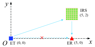
Figure 3: Simulation setup.

V Numerical Results

In this section, numerical results are provided to demonstrate the effectiveness of our proposed joint active and passive beamforming designs exploiting one-bit feedback for our studied IRS-aided WET system. A two-dimensional (2D) coordinate setup is considered where the ET, IRS, and ER are located at $\left({{\text{0 m}},{\text{0 m}}}\right)$, $\left({{\text{5 m}},{\text{2 m}}}\right)$, and $\left({{\text{5 m}},{\text{0 m}}}\right)$, respectively. Both ET-IRS channel and IRS-ER channel are assumed to include large-scale fading and small-scale fading. The large-scale path loss is expressed as $L\left(d\right)={L_{0}}{\left({d/{d_{0}}}\right)^{-\alpha}}$, where $d$ is the link distance, ${L_{0}}=-30{\text{ dB}}$ represents the channel power gain at the reference distance ${d_{0}}=1{\text{ m}}$, and $\alpha=2.2$ is the path loss exponent. To account for small-scale fading, we assume that both ET-IRS and IRS-ER channels follow Rayleigh fading for simplicity. For the distributed-beamforming-based method, the random perturbations are sampled independently and uniformly from $\left({-{{\bar{\Delta}}_{0}},{{\bar{\Delta}}_{0}}}\right)$, i.e., $g\left({{\delta_{i}}}\right)=\frac{1}{{2{{\bar{\Delta}}_{0}}}}$. All the results are averaged over 10 independent channel realizations except for the convergence behaviour of the ACCPM. Unless otherwise specified, we set ${P_{b}}=30{\text{ dBm}}$, $\eta=0.5$, and $N=64$.

V-A Channel-Estimation-Based Method

In Fig. 4, we show the convergence behaviour of the ACCPM. We denote the number of iterations for the ACCPM as $N_{A}$. Recall that the ACCPM is applied to learn a scaled version of the channel matrix ${\bf{P}}\left({{\bf{\bar{v}}}}\right)=\eta{\bf{\bar{H}}}_{c}^{H}{\bf{\bar{v}}}{{{\bf{\bar{v}}}}^{H}}{{{\bf{\bar{H}}}}_{c}}$. To characterize the accuracy of the estimated scaled channel ${{\bf{\tilde{P}}}^{{\rm{esti}}}}$, the normalized error (NE) of ${{\bf{\tilde{P}}}^{{\rm{esti}}}}$ is defined as

$${\mathop{\rm NE}\nolimits}\big{(}{{{{\bf{\tilde{P}}}}^{{\rm{esti}}}}}\big{)}=\frac{{{{\big{\|}{{{{\bf{\tilde{P}}}}^{{\rm{esti,sc}}}}-{\bf{P}}}\big{\|}}_{F}}}}{{{{\left\|{\bf{P}}\right\|}_{F}}}},$$ (45)

where ${{{\bf{\tilde{P}}}}^{{\rm{esti,sc}}}}=\frac{{{{\left\|{\bf{P}}\right\|}_{F}}}}{{{{\big{\|}{{{{\bf{\tilde{P}}}}^{{\rm{esti}}}}}\big{\|}}_{F}}}}{{{\bf{\tilde{P}}}}^{{\rm{esti}}}}$ is the scaled version of ${{{\bf{\tilde{P}}}}^{{\rm{esti}}}}$ such that its Frobenius norm is the same as $\bf{P}$.

It is observed that the ACCPM achieves an asymptotic decreasing estimation error with the number of feedback intervals, which shows its asymptotic convergence in practical implementation. Fluctuations in the performance curves indicate that the NE of the estimated channel matrix is not strictly monotonically decreasing. It is reasonable since the cutting plane formed in each iteration has randomness. We can also see that the convergence speed becomes slower as the number of ET’s antennas increases. This is because the number of the elements in the channel matrix ${\bf{P}}\in{\mathbb{C}^{{M_{t}}\times{M_{t}}}}$ to be estimated increases quadratically with $M_{t}$, and a larger number of elements brings more difficulty of the channel matrix estimation.

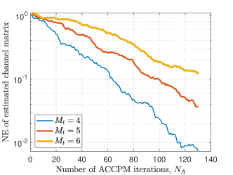
Figure 4: NE of estimated channel matrix by applying the ACCPM versus iteration number $N_{A}$ for different $M_{t}$.

In Fig. 5, we show the performance of our proposed one-bit-feedback-based channel estimation method. We plot the NE of the estimated cascaded channel matrix ${\bf{\bar{H}}}_{c}^{{\rm{LS}}}$ versus the number of feedback intervals in ACCPM under different IRS group sizes. The NE is defined as

$${\mathop{\rm NE}\nolimits}\left({{\bf{\bar{H}}}_{c}^{{\rm{LS}}}}\right)=\arg\mathop{\min}\limits_{\alpha}{\rm{}}\frac{{{{\left\|{{e^{j\alpha}}{\bf{\bar{H}}}_{c}^{{\rm{LS,sc}}}-{{{\bf{\bar{H}}}}_{c}}}\right\|}_{F}}}}{{{{\left\|{{{{\bf{\bar{H}}}}_{c}}}\right\|}_{F}}}},$$ (46)

where ${\bf{\bar{H}}}_{c}^{{\rm{LS,sc}}}=\frac{{{{\left\|{{{{\bf{\bar{H}}}}_{c}}}\right\|}_{F}}}}{{{{\left\|{{\bf{\bar{H}}}_{c}^{{\rm{LS}}}}\right\|}_{F}}}}{\bf{\bar{H}}}_{c}^{{\rm{LS}}}$. For simplicity, we search for $\alpha$ in $\left[{0,2\pi}\right)$ at ${0.5^{\circ}}$ intervals.

First, it is readily seen that a larger number of ACCPM iterations results in a more accurate estimated ${{\bf{\bar{H}}}_{c}}$. This is due to the fact that more ACCPM iterations will result in smaller NE of $\left\{{{\bf{\tilde{p}}}\left({{{{\bf{\bar{v}}}}_{i}}}\right)}\right\}$, whose linear combination, as shown in (III-D), constitutes the estimation of ${{{\bf{\bar{H}}}}_{c}}$. Second, a smaller number of ET’s antenna will accelerate the convergence of the ACCPM, as shown in Fig. 4. Thus, for the same $K$ and $N_{A}$, the NE of the estimated ${{{\bf{\bar{H}}}}_{c}}$ increases with $M_{t}$. Finally, for fixed $M_{t}$, the reduction in IRS group size tends to achieve a more rough estimate of the cascaded channel ${{{\bf{\bar{H}}}}_{c}}$. This can be explained as the convergence rate of the ACCPM depends mainly on the number of ET’s antenna, $M_{t}$, and is not necessarily related to the IRS group size, $K$. Therefore, a larger number of IRS groups leads to a larger cumulative error for the estimated ${\bf{\bar{H}}}_{c}^{{\rm{LS}}}$ with a high probability from (III-D).

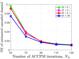
(a) $M_{t}=4$

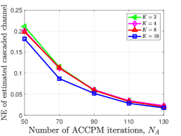
(b) $M_{t}=5$

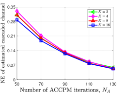
(c) $M_{t}=6$

Figure 5: Performance of the proposed one-bit feedback channel estimation method under different IRS group sizes.

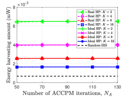
(a) $M_{t}=4$

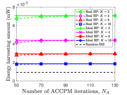
(b) $M_{t}=5$

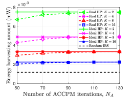
(c) $M_{t}=6$

Figure 6: The amount of harvested power at the ER by applying the proposed channel-estimation-based method for different IRS group sizes.

In Fig. 6, we plot the amount of the harvested energy at the ER versus the number of ACCPM iterations by applying the channel-estimation-based method under different IRS group sizes. We use the term “Real HP” to denote the harvested energy amount obtained by optimizing ${\bf{Q}}$ and ${{\bf{\bar{v}}}}$ based on the estimated cascaded channel ${\bf{\bar{H}}}_{c}^{{\rm{LS}}}$. As a comparison, we plot the ideal harvested energy amount for different IRS group size, termed as “Ideal HP”, where we assume that the cascaded channel ${{{\bf{\bar{H}}}}_{c}}$ is perfectly estimated. Combining with Fig. 5, we can see that a more accurate channel estimation will reduce the gap between the real and ideal harvested energy amounts. In particular, when the NE of the estimated ${{{\bf{\bar{H}}}}_{c}}$ is less than 0.1, the amount of energy harvested at the ER is almost the same as that of the perfect cascaded channel acquisition case. This means that the accuracy of the estimated channel is sufficient when its NE reaches below 0.1. It is also seen that the reduction in IRS group size results in higher harvested power. This is because it helps a finer adjustment of the IRS reflection coefficients. Finally, the performance gain of our proposed channel-estimation-based method can be readily seen compared with the “Random-IRS” case, where the IRS PSs are randomly selected, and the ET adopts the MRT precoding scheme.

V-B Distributed-Beamforming-Based Method

In Fig. 7, we show the convergence behaviour of the distributed beamforming algorithm to optimize ${{\bm{\bar{\theta}}}}$ with $M_{t}=4$, $K=8$, and ${{\bar{\Delta}}_{0}}={2^{\circ}}$. Each of the dash-dotted lines represent the current IRS group PS value, i.e., ${{\bar{\theta}}_{n}},\forall n\in\mathcal{J}$. While the solid lines represent the corresponding theoretical optimal values for each IRS group PS, respectively, i.e., $\bar{\theta}_{n}^{{\rm{opti}}}\left[n\right]=\arg\big{(}{\sum\limits_{j\neq n}{{\bf{\Phi}}\left({n,j}\right){e^{j{{\bar{\theta}}_{j}}\left[n\right]}}}}\big{)},\forall n\in\mathcal{J}$. It is readily seen that although each theoretically optimal PS value varies with the number of feedbacks, each updated IRS group PS gradually approaches its corresponding theoretical optimal value as the number of feedbacks increases, which responses to the statement in Proposition 4 that the distributed beamforming algorithm will eventually converge to a local maximum of problem (32) with probability 1.

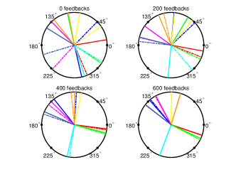
Figure 7: Convergence behaviour of optimizing ${\bm{\bar{\theta}}}$ based on the distributed beamforming method ($M_{t}=4$, $K=8$, and ${{\bar{\Delta}}_{0}}={2^{\circ}}$).

In Fig. 8, we show the convergence behavior of the distributed beamforming algorithm in solving problem (32), for different values of $K$ and ${\bar{\Delta}_{0}}$. First, we can see that for the same $K$ and ${\bar{\Delta}_{0}}$, a smaller IRS group size $K$ leads to an increase in the number of IRS PSs that need to be optimized, and thus a larger number of feedbacks are required to converge. Further, from the two black dashed lines showing the relationship between the required number of feedbacks for convergence and $K$ for ${\bar{\Delta}_{0}}={1^{\circ}}$ and ${\bar{\Delta}_{0}}={2^{\circ}}$, respectively, it can be observed that the number of feedbacks for the distributed beamforming algorithm is sublinear with respect to the number of IRS element groups $J$, which demonstrates its excellent scalability for a large number of IRS PSs optimization. Second, for the same $K$, a larger ${\bar{\Delta}_{0}}$ results in a faster performance improvement for the distributed beamforming algorithm in the initial stage, as a larger range of phase perturbation makes it easier to find higher-quality IRS PS update results. However, it then leveled off at a lower performance, this is due to that the larger phase perturbation range leads to an increase in the proportion of invalid IRS phase shift exploration as the algorithm approaches convergence, and accordingly, the performance can hardly be improved. This inspires us that the value of ${{{\bar{\Delta}}_{0}}}$ can be adapted dynamically during the optimization. For example, the value of ${{{\bar{\Delta}}_{0}}}$ can be decreased linearly as the reduction of the update frequency of ${{\bm{\bar{\theta}}}}$.

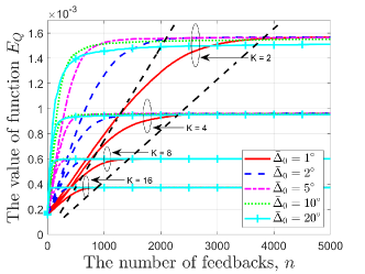
Figure 8: Convergence behaviour of solving problem (32) by applying the distributed beamforming method for different values of $K$ and ${{\bar{\Delta}}_{0}}$ ($M_{t}=4$).

In Fig. 9, we plot the ER’s harvested energy amount obtained by applying the distributed-beamforming-based method for different feedback numbers of ACCPM (in the second stage) and distributed beamforming algorithm (in the first stage) with $K=8$ and ${{\bar{\Delta}}_{0}}={2^{\circ}}$. We use ${N_{D}}$ to denote the feedback number for the distributed beamforming algorithm. Obviously, the amount of the harvested energy increases with the feedback numbers of both distributed beamforming procedure and ACCPM. For all the $M_{t}$ settings, the performance curves corresponding to ${N_{D}}$ set to $600$ and $700$, respectively, are very close for all numbers of the ACCPM feedbacks, indicating that for the distributed beamforming algorithm, the performance is basically saturated at the current parameter setting ($J=8$) when the number of feedbacks reaches $700$. Moreover, for a fixed ${N_{D}}$, the number of ACCPM feedbacks required for convergence increases with $M_{t}$, which is consistent with the convergence behaviour of the ACCPM shown in Fig. 4. In addition, the performance gain of the proposed distributed-beamforming-based method is verified by comparing with the benchmark scheme, where the IRS PSs are randomly selected and the transmit covariance matrix at the ET is set to ${\bf{Q}}=\frac{{{P_{b}}}}{{{M_{t}}}}{{\bf{I}}_{{M_{t}}}}$.

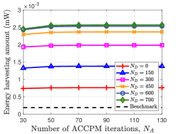
(a) $M_{t}=4$

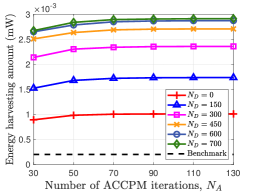
(b) $M_{t}=5$

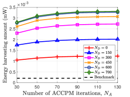
(c) $M_{t}=6$

Figure 9: Harvested energy amount by applying the distributed-beamforming-based method for different feedback numbers of ACCPM and distributed beamforming algorithm ($K=8$, ${\bar{\Delta}_{0}}={2^{\circ}}$).

In Fig. 10, we compare the amount of the harvested energy obtained by our proposed joint beamforming design schemes with two benchmark schemes, namely, the beam training scheme and the random beamforming scheme. The simulation parameters are set as follows: 1) CE: for the channel-estimation-based method, the iteration number of ACCPM is set to $N_{A}=130$; 2) DBF: for the distributed-beamforming-based method, we set the parameters of the first stage to $N_{D}=5000$ and ${\bar{\Delta}_{0}}{\rm{=}}{2^{\circ}}$, and the parameter of the second stage to $N_{A}=130$; 3) BT: for the beam training scheme, the directional beams of the ET and IRS are selected from discrete Fourier Transform (DFT) codebook, and the entries of the transmit beamforming vector at the ET are set to phase-only complex variables with invariable amplitude [23]. Moreover, exhaustive search is applied to find the optimal beam pair; 4) RBF: for the random beamforming scheme, we set ${\bf{Q}}=\frac{{{P_{b}}}}{{{M_{t}}}}{\bf{I}}$, and the IRS PSs are randomly selected. From Fig. 10, our proposed schemes achieve superior performance over the other schemes. Moreover, the channel-estimation-based scheme achieves almost the same performance as the distributed-beamforming-based scheme. The reason for the performance gap between the proposed schemes and the beam training scheme, especially for a smaller $K$, is that Rayleigh fading is adopted as the small-scale fading for both ET-IRS and IRS-ER channels, which is not sparse, thus leading to a significant performance loss for the beam training scheme. The performance of the random beamforming scheme remains almost unchanged with $M_{t}$ and $K$, which demonstrates the importance of joint active and passive beamforming design for IRS-aided wireless system.

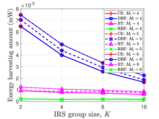
Figure 10: The amount of harvested energy versus IRS group sizes for different $M_{t}$ under different schemes.

VI Conclusion

In this paper, we proposed two novel joint active and passive beamforming design schemes, namely, the channel-estimation-based method and the distributed-beamforming-based method, for an IRS-aided WET system exploiting only one-bit feedback from the ER to the ET. Specifically, for the channel-estimation-based method, with the predetermined IRS PS matrix, we first estimated the scaled cascaded ET-IRS-ER channel by continually adjusting the transmit covariance matrix at the ET based on the ACCPM. Then, the joint beamforming design was performed based on the estimated cascaded channel by applying the existing optimization methods. While for the distributed-beamforming-based method, we first applied the distributed beamforming algorithm to optimize the IRS refection coefficients without knowing any involved CSI, which theoretically proven to converge to a local optimum almost surely. Then, for the given optimized IRS PSs, the ET’s transmit covariance matrix was calculated according to the effective ET-ER channel learned by applying the ACCPM only once. Simulation results demonstrated the effectiveness of our proposed one-bit-feedback-based joint beamforming design schemes. More importantly, the proposed schemes were shown to be more appealing compared to existing pilot-based beamforming method and beam training method in terms of the ER’s hardware complexity requirement and system performance, respectively. In particular, the proposed one-bit-feedback-based cascaded channel estimation method was also validated to have high accuracy.

Appendix A Proof of Proposition 1

The idea behind the proof is to resort to the derivative of ${E_{h}}\left(\vartheta\right)$ with respect to $\vartheta$. First, we have

$$\frac{{\partial{E_{h}}}}{{\partial\vartheta}}= 2\Re\left\{{j\left({{R_{i,j}}{e^{-j\vartheta}}{\bf{\tilde{p}}}_{i}^{H}+{\bf{\tilde{p}}}_{j}^{H}}\right)}\right.$$

$$\big{.}{\left({{R_{i,j}}{e^{j{\delta_{i,j}}}}{{{\bf{\tilde{p}}}}_{i}}+{{{\bf{\tilde{p}}}}_{j}}}\right)\big{(}{{e^{j\left({\vartheta-{\delta_{i,j}}}\right)}}-1}\big{)}}\big{\}}\times\psi\left(\vartheta\right),$$ (47)

where $\psi\left(\vartheta\right)=\frac{{R_{i,j}^{2}\big{(}{{{\left\|{{{{\bf{\tilde{p}}}}_{i}}}\right\|}^{2}}{{\left\|{{{{\bf{\tilde{p}}}}_{j}}}\right\|}^{2}}-{{\left|{{\bf{\tilde{p}}}_{i}^{H}{{{\bf{\tilde{p}}}}_{j}}}\right|}^{2}}}\big{)}}}{{{{\left|{{{\left({{R_{i,j}}{e^{j\vartheta}}{{{\bf{\tilde{p}}}}_{i}}+{{{\bf{\tilde{p}}}}_{j}}}\right)}^{H}}\left({{R_{i,j}}{e^{j\vartheta}}{{{\bf{\tilde{p}}}}_{i}}+{{{\bf{\tilde{p}}}}_{j}}}\right)}\right|}^{2}}}}$ is a positive real number, ${{{\bf{\tilde{p}}}}_{i}}$ and ${{{\bf{\tilde{p}}}}_{j}}$ are short for ${\bf{\tilde{p}}}\left({{{{\bf{\bar{v}}}}_{i}}}\right)$ and ${\bf{\tilde{p}}}\left({{{{\bf{\bar{v}}}}_{j}}}\right)$, respectively, and we define ${R_{i,j}}=\left|{{\gamma_{i}}}\right|/\left|{{\gamma_{j}}}\right|$, and ${\delta_{i,j}}=\angle{\gamma_{i}}-\angle{\gamma_{j}}$. By setting the derivative of ${E_{h}}\left(\vartheta\right)$ w.r.t $\vartheta$ to zero, we have

$$\frac{{\partial{E_{h}}}}{{\partial\vartheta}}=0 \Rightarrow 2\Re\left\{{j\left({{R_{i,j}}{e^{-j\vartheta}}{\bf{\tilde{p}}}_{i}^{H}+{\bf{\tilde{p}}}_{j}^{H}}\right)}\right.$$

$$\big{.}{\left({{R_{i,j}}{e^{j{\delta_{i,j}}}}{{{\bf{\tilde{p}}}}_{i}}+{{{\bf{\tilde{p}}}}_{j}}}\right)\big{(}{{e^{j\left({\vartheta-{\delta_{i,j}}}\right)}}-1}\big{)}}\big{\}}=0$$

$$\Rightarrow f\left(\vartheta\right)=0,$$ (48)

where

$$f\left(\vartheta\right) =\big{(}{{{\left\|{{{{\bf{\tilde{p}}}}_{j}}}\right\|}^{2}}+R_{i,j}^{2}{{\left\|{{{{\bf{\tilde{p}}}}_{i}}}\right\|}^{2}}}\big{)}\sin\left({\vartheta-{\delta_{i,j}}}\right)$$

$$+2{R_{i,j}}\Re\left\{{{\bf{\tilde{p}}}_{i}^{H}{{{\bf{\tilde{p}}}}_{j}}}\right\}\sin\vartheta-2{R_{i,j}}\sin{\delta_{i,j}}\Re\left\{{{\bf{\tilde{p}}}_{i}^{H}{{{\bf{\tilde{p}}}}_{j}}}\right\}$$

$$=A\sin\big{(}{\vartheta-\frac{{{\delta_{i,j}}}}{2}+\phi}\big{)}-{A_{1}}\sin{\delta_{i,j}},$$ (49)

with $A=\sqrt{A_{1}^{2}+A_{2}^{2}+2{A_{1}}{A_{2}}\cos\left({{\delta_{i,j}}}\right)}$, ${A_{1}}=2{R_{i,j}}\Re\left\{{{\bf{\tilde{p}}}_{i}^{H}{{{\bf{\tilde{p}}}}_{j}}}\right\}$, ${A_{2}}={{{\left\|{{{{\bf{\tilde{p}}}}_{j}}}\right\|}^{2}}+R_{i,j}^{2}{{\left\|{{{{\bf{\tilde{p}}}}_{i}}}\right\|}^{2}}}$, and $\phi$ satisfies the equation $\tan\phi=\frac{{{A_{1}}-{A_{2}}}}{{{A_{1}}+{A_{2}}}}\tan\big{(}{\frac{{{\delta_{i,j}}}}{2}}\big{)}$. Mathematically, $f\left(\vartheta\right)=0$ is equivalent to the intersection of ${f_{1}}\left(\vartheta\right)=A\sin\big{(}{\vartheta-\frac{{{\delta_{i,j}}}}{2}+\phi}\big{)}$ and ${f_{2}}={A_{1}}\sin{\delta_{i,j}}$. Since

$${A^{2}}-A_{1}^{2}{\sin^{2}}{\delta_{i,j}}$$ (50a)

$$=A_{1}^{2}{\cos^{2}}{\delta_{i,j}}+A_{2}^{2}+2{A_{1}}{A_{2}}\cos\left({{\delta_{i,j}}}\right)$$ (50b)

$$\mathop{\geq}\limits^{\left(a\right)}A_{1}^{2}+A_{2}^{2}-2\left|{{A_{1}}}\right|{A_{2}}>0,$$ (50c)

where $\left(a\right)$ is due to the fact that the minimum value of (50b) is achieved when $\cos\left({{\delta_{i,j}}}\right)=-\frac{{{A_{1}}}}{{\left|{{A_{1}}}\right|}}$, we have

$$\left|A\right|>\left|{{A_{1}}\sin\left({{\delta_{i,j}}}\right)}\right|.$$ (51)

Thus, as $\vartheta$ varies from $0$ to $2\pi$, ${f_{1}}\left(\vartheta\right)$ and ${f_{2}}$ have two intersection points, i.e., there are two extreme points for ${E_{h}}\left(\vartheta\right)$ within the interval of $\left[{0,2\pi}\right)$, one is the local maximum point and the other is the local minimum point. Moreover, since ${E_{h}}\left(\vartheta\right)$ is a periodic function satisfying ${E_{h}}\left(0\right)={E_{h}}\left({2\pi}\right)$, we can conclude that the local maximum is the global maximum. It is readily seen that the global maximum is obtained when $\vartheta=\angle{\gamma_{i}}-\angle{\gamma_{j}}$, thus the value of $\angle{\gamma_{i}}-\angle{\gamma_{j}}$ can be obtained by finding the unique local maximum point of ${E_{h}}\left(\vartheta\right)$ within the interval of $\left[{0,2\pi}\right)$. This completes the proof.

Appendix B Proof of Proposition 3

Denote the $n$th entry of ${\bf{\bar{v}}}$ as ${{\bar{v}}_{n}},\forall n\in\mathcal{J}$. The function ${E_{Q}}\left({{\bf{\bar{v}}}}\right)$ in (32a) can be expanded as

$${E_{Q}}\left({{\bf{\bar{v}}}}\right)=\sum\limits_{i=1}^{J}{{\bf{\Phi}}\left({i,i}\right)}+\sum\limits_{i=1}^{J}{\sum\limits_{j=1}^{i-1}{2\Re\left\{{{\bar{v}_{i}^{*}}{\bf{\Phi}}\left({i,j}\right){{\bar{v}}_{j}}}\right\}}}.$$ (52)

Then, the function of ${E_{Q}}\left({{\bf{\bar{v}}}}\right)$ with respect to the $n$th entry of ${{\bf{\bar{v}}}}$, i.e., ${{{{\bar{v}}}}_{n}}$, can be written as

$${E_{Q}}\left({{\bar{v}}_{n}}\right)=2\Re\big{\{}{{{\bar{v}}}_{n}^{*}\sum\limits_{j\neq n}{{\bf{\Phi}}\left({n,j}\right){{{{\bar{v}}}}_{j}}}}\big{\}}+{\text{constant}}.$$ (53)

Applying the chain rule, the derivative of the function ${E_{Q}}\left({{\bf{\bar{v}}}\left({{\bm{\bar{\theta}}}}\right)}\right)$ with respect to ${{{{\bar{\theta}}}}_{n}}$ is given by

$$\frac{{\partial{E_{Q}}\left({{\bf{\bar{v}}}\left({{\bm{\bar{\theta}}}}\right)}\right)}}{{\partial{{\bar{\theta}}_{n}}}} =\frac{{\partial{E_{Q}}\left({{\bf{\bar{v}}}}\right)}}{{\partial{{\bar{v}}_{n}}}}\frac{{\partial{{\bar{v}}_{n}}}}{{\partial{{\bar{\theta}}_{n}}}}+\frac{{\partial{E_{Q}}\left({{\bf{\bar{v}}}}\right)}}{{\partial\bar{v}_{n}^{*}}}\frac{{\partial\bar{v}_{n}^{*}}}{{\partial{{\bar{\theta}}_{n}}}}$$

$$=2\Im\big{\{}{{e^{-j{{\bar{\theta}}_{n}}}}\big{(}{\sum\limits_{j\neq n}{{\bf{\Phi}}\left({n,j}\right){{\bar{v}}_{j}}}}\big{)}}\big{\}}.$$ (54)

For the second term on the right hand side of (52), we have

$$\sum\limits_{i=1}^{J}{\sum\limits_{j=1}^{i-1}{2\Re\left\{{\bar{v}_{i}^{*}{\bf{\Phi}}\left({i,j}\right){{\bar{v}}_{j}}}\right\}}}=2\sum\limits_{i=1}^{J}{\big{|}{\sum\limits_{j=1}^{i-1}{{\bf{\Phi}}\left({i,j}\right){{\bar{v}}_{j}}}}\big{|}\cos\left({{\varphi_{i}}}\right)},$$ (55)

where ${\varphi_{i}}=\arg\big{(}{\sum\limits_{j=1}^{i-1}{{\bf{\Phi}}\left({i,j}\right){{\bar{v}}_{j}}}}\big{)}-\bar{\theta}_{i}$ is the angle difference between the current ${{\bar{\theta}}_{i}}$ and the local maximum. For simplicity, we assume that $\left\{{\left|{{\varphi_{i}}}\right|}\right\}_{i=1}^{J}$ are sorted such that $\left|{{\varphi_{1}}}\right|\geq\left|{{\varphi_{2}}}\right|\geq\cdots\geq\left|{{\varphi_{J}}}\right|$. Thus we have

$$\sum\limits_{i=1}^{J}{\sum\limits_{j=1}^{i-1}{2\Re\left\{{\bar{v}_{i}^{*}{\bf{\Phi}}\left({i,j}\right){{\bar{v}}_{j}}}\right\}}}\geq 2\cos\left({{\varphi_{1}}}\right)\sum\limits_{i=1}^{J}{\big{|}{\sum\limits_{j=1}^{i-1}{{\bf{\Phi}}\left({i,j}\right){{\bar{v}}_{j}}}}\big{|}}.$$ (56)

Assuming that ${E_{Q}}\left({{\bf{\bar{v}}}\left({{\bm{\bar{\theta}}}}\right)}\right)\leq{Y^{{\rm{opt}}}}-\epsilon$, from (B) we conclude that $\left|{{\varphi_{1}}}\right|>0$. Further, we have

$$\sum\limits_{i=1}^{J}{{\bf{\Phi}}\left({i,i}\right)}+2\cos\left({{\varphi_{1}}}\right)\sum\limits_{i=1}^{J}{\big{|}{\sum\limits_{j=1}^{i-1}{{\bf{\Phi}}\left({i,j}\right){{\bar{v}}_{j}}}}\big{|}}\leq{Y^{{\rm{opt}}}}-\epsilon$$

$$\Rightarrow\left|{{\varphi_{1}}}\right|\geq{\phi_{\epsilon}}\buildrel\Delta\over{=}\arccos\left({\frac{{{Y^{{\rm{opt}}}}-\epsilon-{\sum\limits_{i}{{\bf{\Phi}}\left({i,i}\right)}}}}{{2\sum\limits_{i=1}^{J}{\big{|}{\sum\limits_{j=1}^{i-1}{{\bf{\Phi}}\left({i,j}\right){{\bar{v}}_{j}}}}\big{|}}}}}\right).$$ (57)

For ease of analysis, we treat the perturbation $\bm{\delta}$ applied to ${{\bm{\bar{\theta}}}}$ as each perturbation $\delta_{i}$ applied to ${{\bar{\theta}}_{i}}$ one by one. Now, we choose a phase perturbation $\delta_{1}$ such that $\left|{{\varphi_{1}}}\right|$ is decreased. This makes the amount of harvested energy at the ER increase. Without loss of generality, we assume ${\varphi_{1}}>0$, then we need to choose a $\delta_{1}>0$. Consider ${\delta_{1}}\in\left({\frac{{{\Delta_{0}}}}{2},{\Delta_{0}}}\right)$, we have

$${\rho_{1}}\buildrel\Delta\over{=}\Pr\big{(}{\frac{{{\Delta_{0}}}}{2}\leq{\delta_{1}}\leq{\Delta_{0}}}\big{)}=\int_{\frac{{{\Delta_{0}}}}{2}}^{{\Delta_{0}}}{g\left(x\right)dx}>0,$$ (58)

and from (53), we obtain

$${E_{Q}}\left({{{\bar{v}}_{1}}\left({{{\bar{\theta}}_{1}}+{\delta_{1}}}\right)}\right)-{E_{Q}}\left({{{\bar{v}}_{1}}\left({{{\bar{\theta}}_{1}}}\right)}\right)$$

$$=2\Re\big{\{}{\big{(}{{e^{-j\left({{{\bar{\theta}}_{1}}+{\delta_{1}}}\right)}}-{e^{-j{{\bar{\theta}}_{1}}}}}\big{)}\sum\limits_{j\neq 1}{{\bf{\Phi}}\left({n,j}\right){{\bar{v}}_{j}}}}\big{\}}$$

$$=2\big{|}{\sum\limits_{j\neq 1}{{\bf{\Phi}}\left({n,j}\right){{\bar{v}}_{j}}}}\big{|}\left({\cos\left({{\varphi_{1}}-{\delta_{1}}}\right)-\cos\left({{\varphi_{1}}}\right)}\right)$$

$$>2\big{|}{\sum\limits_{j\neq 1}{{\bf{\Phi}}\left({n,j}\right){{\bar{v}}_{j}}}}\big{|}\frac{{{\Delta_{0}}}}{2}\sin\big{(}{{\phi_{\epsilon}}-\frac{{{\Delta_{0}}}}{2}}\big{)}=2{\epsilon_{1}},$$ (59)

where ${\epsilon_{1}}\buildrel\Delta\over{=}\frac{{{\Delta_{0}}}}{2}\big{|}{\sum\limits_{j\neq 1}{{\bf{\Phi}}\left({n,j}\right){{\bar{v}}_{j}}}}\big{|}\sin\left({{\phi_{\epsilon}}-\frac{{{\Delta_{0}}}}{2}}\right)$. To obtain a positive value of ${E_{Q}}\left({{\bf{\bar{v}}}\left({{\bm{\bar{\theta}}}+{\bm{\delta}}}\right)}\right)-{E_{Q}}\left({{\bf{\bar{v}}}\left({{\bm{\bar{\theta}}}}\right)}\right)$, a safe measure is to ensure that the other IRS phase shift perturbations ${\left\{{{\delta_{j}}}\right\}_{j\neq 1}}$ are small enough compared to $\delta_{1}$. From (52), we have (B), which is shown at the top of the next page. Since ${E_{Q}}\left({{\bf{\bar{v}}}\left({{\bm{\bar{\theta}}}}\right)}\right)$ is continuous in each of the phases ${{\bar{\theta}}_{i}}$, we can always find a $\epsilon_{1}>0,\forall i>1$, to satisfy (61), which is also shown at the top of the next page. Due to

$${E_{Q}}\left({{\bf{\bar{v}}}\left({{\bm{\bar{\theta}}}+{\bm{\delta}}}\right)}\right)-{E_{Q}}\left({{\bf{\bar{v}}}\left({{\bm{\bar{\theta}}}}\right)}\right)$$

$$={E_{Q}}\left({{{\bar{v}}_{1}}\left({{{\bar{\theta}}_{1}}+{\delta_{1}}}\right)}\right)-{E_{Q}}\left({{{\bar{v}}_{1}}\left({{{\bar{\theta}}_{1}}}\right)}\right)+\sum\limits_{i>1}{{E_{Q}}\left({{{\bar{v}}_{i}}\left({{{\bar{\theta}}_{i}}+{\delta_{i}}}\right)|{{\bar{\theta}}_{j}}\leftarrow{{\bar{\theta}}_{j}}+{\delta_{j}},\forall j<i}\right)-{E_{Q}}\left({{{\bar{v}}_{i}}\left({{{\bar{\theta}}_{i}}}\right)|{{\bar{\theta}}_{j}}\leftarrow{{\bar{\theta}}_{j}}+{\delta_{j}},\forall j<i}\right)}$$

$$>2{\epsilon_{1}}+2\Re\Big{\{}{\sum\limits_{i>1}{{e^{-j{{\bar{\theta}}_{i}}}}\left({{e^{-j{\delta_{i}}}}-1}\right)\Big{(}{\sum\limits_{j<i}{{\bf{\Phi}}\left({i,j}\right){e^{j\left({{{\bar{\theta}}_{j}}+{\delta_{j}}}\right)}}}+\sum\limits_{j>i}{{\bf{\Phi}}\left({i,j}\right){e^{j{{\bar{\theta}}_{j}}}}}}\Big{)}}}\Big{\}}.$$ (60)

$$\bigg{|}{2\Re\Big{\{}{{e^{-j{{\bar{\theta}}_{i}}}}\left({{e^{-j{\delta_{i}}}}-1}\right)\Big{(}{\sum\limits_{j<i}{{\bf{\Phi}}\left({i,j}\right){e^{j\left({{{\bar{\theta}}_{j}}+{\delta_{j}}}\right)}}}+\sum\limits_{j>i}{{\bf{\Phi}}\left({i,j}\right){e^{j{{\bar{\theta}}_{j}}}}}}\Big{)}}\Big{\}}}\bigg{|}<\frac{{{\epsilon_{1}}}}{{J-1}},\forall\big{|}{{\delta_{i}}}\big{|}<{\epsilon_{i}},i>1.$$ (61)

$$\left({{\text{The left hand side of }}\left(\text{\ref{eq_ige1}}\right)}\right)$$

$$\leq 2\big{|}{{e^{-j{{\bar{\theta}}_{i}}}}\left({{e^{-j{\delta_{i}}}}-1}\right)}\big{|}$$

$$\qquad\times\Big{|}{\Big{(}{\sum\limits_{j<i}{{\bf{\Phi}}\left({i,j}\right){e^{j\left({{{\bar{\theta}}_{j}}+{\delta_{j}}}\right)}}}+\sum\limits_{j>i}{{\bf{\Phi}}\left({i,j}\right){e^{j{{\bar{\theta}}_{j}}}}}}\Big{)}}\Big{|}$$

$$\leq 4\big{|}{\sin\big{(}{\frac{{{\delta_{i}}}}{2}}\big{)}}\big{|}\sum\limits_{j\neq i}{\left|{{\bf{\Phi}}\left({i,j}\right)}\right|},$$ (62)

it can be readily seen that ${\epsilon_{i}}=2\arcsin\big{(}{\frac{{{\epsilon_{1}}}}{{4\left({J-1}\right)\sum\nolimits_{j\neq i}{\left|{{\bf{\Phi}}\left({i,j}\right)}\right|}}}}\big{)}$ satisfies (61). With ${\left\{{{\delta_{i}}}\right\}_{i>1}}$ chosen that satisfies (61), we have

$${E_{Q}}\left({{\bf{\bar{v}}}\left({{\bm{\bar{\theta}}}+{\bm{\delta}}}\right)}\right)-{E_{Q}}\left({{\bf{\bar{v}}}\left({{\bm{\bar{\theta}}}}\right)}\right)\geq{\epsilon_{1}}.$$ (63)

Moreover, since the PDF $g\left({{\delta_{i}}}\right)$ is bounded away from zero in each of the intervals $\left({-{\epsilon_{i}},{\epsilon_{i}}}\right)$, the probability $\rho_{i}$ of choosing $\delta_{i}$ to satisfies (61) is nonzero, i.e., $\rho_{i}>0$. Finally, we can see that all the entries in $\left\{{{\delta_{i}}}\right\}_{i=1}^{J}$ are chosen independently, thus (63) holds at least with probability $\rho=\prod\nolimits_{i}{{\rho_{i}}}>0$. This thus completes the proof.

References

• [1] C.-X. Wang, X. You, X. Gao et al., “On the road to 6G: Visions, requirements, key technologies, and testbeds,” IEEE Commun. Surveys Tuts., vol. 25, no. 2, pp. 905–974, Feb. 2023.
• [2] Z. Chen, G. Chen, J. Tang et al., “Reconfigurable-intelligent-surface-assisted B5G/6G wireless communications: Challenges, solution, and future opportunities,” IEEE Commun. Mag., vol. 61, no. 1, pp. 16–22, Jan. 2023.
• [3] C. Pan, H. Ren, K. Wang et al., “Reconfigurable intelligent surfaces for 6G systems: Principles, applications, and research directions,” IEEE Commun. Mag., vol. 59, no. 6, pp. 14–20, Jun. 2021.
• [4] S. Basharat, S. A. Hassan, H. Pervaiz et al., “Reconfigurable intelligent surfaces: Potentials, applications, and challenges for 6G wireless networks,” IEEE Wireless Commun., vol. 28, no. 6, pp. 184–191, Dec. 2021.
• [5] Q. Wu, S. Zhang, B. Zheng, C. You, and R. Zhang, “Intelligent reflecting surface-aided wireless communications: A tutorial,” IEEE Trans. Commun., vol. 69, no. 5, pp. 3313–3351, May 2021.
• [6] X. Mu, Y. Liu, L. Guo, J. Lin, and R. Schober, “Simultaneously transmitting and reflecting (STAR) RIS aided wireless communications,” IEEE Trans. Wireless Commun., vol. 21, no. 5, pp. 3083–3098, May 2022.
• [7] T. Ji, M. Hua, C. Li, Y. Huang, and L. Yang, “Robust max-min fairness transmission design for IRS-aided wireless network considering user location uncertainty,” IEEE Trans. Commun., vol. 71, no. 8, pp. 4678–4693, Aug. 2023.
• [8] Y. Wu, F. Zhou, W. Wu et al., “Multi-objective optimization for spectrum and energy efficiency tradeoff in IRS-assisted CRNs with NOMA,” IEEE Trans. Wireless Commun., vol. 21, no. 8, pp. 6627–6642, Aug. 2022.
• [9] J. Chen, Y. Xie, X. Mu et al., “Energy efficient resource allocation for IRS assisted CoMP systems,” IEEE Trans. Wireless Commun., vol. 21, no. 7, pp. 5688–5702, Jul. 2022.
• [10] M. Hua, Q. Wu, C. He et al., “Joint active and passive beamforming design for IRS-aided radar-communication,” IEEE Trans. Wireless Commun., vol. 22, no. 4, pp. 2278–2294, Apr. 2023.
• [11] W. Ma, L. Zhu, and R. Zhang, “Passive beamforming for 3-D coverage in IRS-assisted communications,” IEEE Wireless Commun. Lett., vol. 11, no. 8, pp. 1763–1767, Aug. 2022.
• [12] X. Shi, N. Deng, N. Zhao, and D. Niyato, “Coverage enhancement in millimeter-wave cellular networks via distributed IRSs,” IEEE Trans. Commun., vol. 71, no. 2, pp. 1153–1167, Feb. 2023.
• [13] S. Zeng, H. Zhang, B. Di et al., “Reconfigurable intelligent surface (RIS) assisted wireless coverage extension: RIS orientation and location optimization,” IEEE Commun. Lett., vol. 25, no. 1, pp. 269–273, Jan. 2021.
• [14] H.-M. Wang, J. Bai, and L. Dong, “Intelligent reflecting surfaces assisted secure transmission without eavesdropper’s CSI,” IEEE Signal Process. Lett., vol. 27, pp. 1300–1304, 2020.
• [15] J. Qiao, C. Zhang, A. Dong et al., “Securing intelligent reflecting surface assisted terahertz systems,” IEEE Trans. Veh. Technol., vol. 71, no. 8, pp. 8519–8533, Aug. 2022.
• [16] A. L. Swindlehurst, G. Zhou, R. Liu et al., “Channel estimation with reconfigurable intelligent surfaces—A general framework,” Proc. IEEE, vol. 110, no. 9, pp. 1312–1338, Sep. 2022.
• [17] T. L. Jensen and E. De Carvalho, “An optimal channel estimation scheme for intelligent reflecting surfaces based on a minimum variance unbiased estimator,” in Proc. IEEE Int. Conf. Acoust. Speech Signal Process., 2020, pp. 5000–5004.
• [18] C. Liu, X. Liu, D. W. K. Ng, and J. Yuan, “Deep residual learning for channel estimation in intelligent reflecting surface-assisted multi-user communications,” IEEE Trans. Wireless Commun., vol. 21, no. 2, pp. 898–912, Feb. 2022.
• [19] Z. Zhang, T. Ji, H. Shi et al., “A self-supervised learning-based channel estimation for IRS-aided communication without ground truth,” IEEE Trans. Wireless Commun., vol. 22, no. 8, pp. 5446–5460, Aug. 2023.
• [20] P. Wang, J. Fang, H. Duan, and H. Li, “Compressed channel estimation for intelligent reflecting surface-assisted millimeter wave systems,” IEEE Signal Process. Lett., vol. 27, pp. 905–909, 2020.
• [21] G. T. de Araújo, A. L. F. de Almeida, and R. Boyer, “Channel estimation for intelligent reflecting surface assisted MIMO systems: A tensor modeling approach,” IEEE J. Sel. Topics Signal Process., vol. 15, no. 3, pp. 789–802, Apr. 2021.
• [22] J. Wang, W. Tang, S. Jin et al., “Hierarchical codebook-based beam training for RIS-assisted mmWave communication systems,” IEEE Trans. Commun., vol. 71, no. 6, pp. 3650–3662, Jun. 2023.
• [23] W. Wang and W. Zhang, “Joint beam training and positioning for intelligent reflecting surfaces assisted millimeter wave communications,” IEEE Trans. Wireless Commun., vol. 20, no. 10, pp. 6282–6297, Oct. 2021.
• [24] B. Ning, Z. Chen, W. Chen et al., “Terahertz multi-user massive mimo with intelligent reflecting surface: Beam training and hybrid beamforming,” IEEE Trans. Veh. Technol., vol. 70, no. 2, pp. 1376–1393, Feb. 2021.
• [25] X. Zhou, R. Zhang, and C. K. Ho, “Wireless information and power transfer: Architecture design and rate-energy tradeoff,” IEEE Trans. Commun., vol. 61, no. 11, pp. 4754–4767, Nov. 2013.
• [26] J. Xu and R. Zhang, “Energy beamforming with one-bit feedback,” IEEE Trans. Signal Process., vol. 62, no. 20, pp. 5370–5381, Oct. 2014.
• [27] B. Gopalakrishnan and N. D. Sidiropoulos, “High performance adaptive algorithms for single-group multicast beamforming,” IEEE Trans. Signal Process., vol. 63, no. 16, pp. 4373–4384, Aug. 2015.
• [28] R. Mudumbai, J. Hespanha, U. Madhow, and G. Barriac, “Distributed transmit beamforming using feedback control,” IEEE Trans. Inf. Theory, vol. 56, no. 1, pp. 411–426, Jan. 2010.
• [29] Y. Yang, B. Zheng, S. Zhang, and R. Zhang, “Intelligent reflecting surface meets OFDM: Protocol design and rate maximization,” IEEE Trans. Commun., vol. 68, no. 7, pp. 4522–4535, Jul. 2020.
• [30] M. Biguesh and A. Gershman, “Training-based MIMO channel estimation: A study of estimator tradeoffs and optimal training signals,” IEEE Trans. Signal Process., vol. 54, no. 3, pp. 884–893, Mar. 2006.
• [31] J. Sun, K.-C. Toh, and G. Zhao, “An analytic center cutting plane method for semidefinite feasibility problems,” Math. Oper. Res., vol. 27, no. 2, pp. 332–346, 2002.
• [32] Z. Wang, L. Liu, and S. Cui, “Channel estimation for intelligent reflecting surface assisted multiuser communications: Framework, algorithms, and analysis,” IEEE Trans. Wireless Commun., vol. 19, no. 10, pp. 6607–6620, Oct. 2020.
• [33] R. Zhang and C. K. Ho, “MIMO broadcasting for simultaneous wireless information and power transfer,” IEEE Trans. Wireless Commun., vol. 12, no. 5, pp. 1989–2001, May 2013.
• [34] C. Pan, G. Zhou, K. Zhi et al., “An overview of signal processing techniques for RIS/IRS-aided wireless systems,” IEEE J. Sel. Topics Signal Process., vol. 16, no. 5, pp. 883–917, Aug. 2022.
• [35] R. Mudumbai, D. R. Brown Iii, U. Madhow, and H. V. Poor, “Distributed transmit beamforming: challenges and recent progress,” IEEE Commun. Mag., vol. 47, no. 2, pp. 102–110, Feb. 2009.