Solving quantum impurity problems on the L-shaped Kadanoff-Baym contour

Abstract

The path integral formalism is the building block of many powerful numerical methods for quantum impurity problems. However, existing fermionic path integral based numerical calculations have only been performed in either the imaginary-time or the real-time axis, while the most generic scenario formulated on the L-shaped Kadanoff-Baym contour is left unexplored. In this work, we extended the recently developed Grassmann time-evolving matrix product operator (GTEMPO) method to solve quantum impurity problems directly on the Kadanoff-Baym contour. The resulting method is numerically exact, with only two sources of numerical errors, e.g., the time discretization error and the matrix product state bond truncation error, which can both be well controlled. The accuracy of this method is numerically demonstrated against exact solutions in the noninteracting case, and against existing calculations on the real- and imaginary-time axes for the single-orbital Anderson impurity model. Our method is a perfect benchmarking baseline for its alternatives which often employ less-controlled approximations, and can also be used as a real-time impurity solver in dynamical mean field theory and its non-equilibrium extension.

I Introduction

The quantum impurity problem (QIP), which considers an impurity of a few energy levels that is coupled to a continuous noninteracting bath, represents a cornerstone in condensed matter physics for studying strongly correlated effects [1] and open quantum effects [2]. It is also the building block in quantum embedding methods such as the dynamical mean field theory (DMFT) [3, 4] and non-equilibrium DMFT [5].

The observables of interest in solving QIPs are the multi-time correlations of the impurity. Existing numerical approaches for QIPs can be primarily divided into two categories: (1) the wave-function based approach and (2) the path integral (PI) based approach. In the first category, one discretizes the bath into a finite number of modes and parameterizes the impurity-bath wave function with some ansatz, then one can compute the multi-time impurity correlations by performing real-time evolution of the wave function ansatz. The representative methods in the first category include the exact diagonalization [6, 7, 8, 9, 10, 11, 12], numerical renormalization group [13, 14, 15, 16, 17, 18, 19, 20, 21] and matrix product state (MPS) based methods [22, 23, 24, 25, 26, 27, 28, 29, 30, 31, 32, 33]. The scalability or accuracy of these methods are basically limited by the discretization of the continuous bath.

In the second category, the starting point is the PI of the impurity, where the bath has already been integrated out analytically via the Feynman-Vernon influence functional (IF) [34] and one is left only with the impurity degrees of freedom in the temporal domain. Most outstandingly, the class of continuous-time Quantum Monte Carlo (CTQMC) methods directly draw samples from the perturbative expansion of the PI, which could efficiently yield exact results in the imaginary-time axis [4, 35, 36, 37, 38, 39, 40]. QMC calculations in the real-time axis are not as successful, but have been improved significantly in recent years with advanced time-domain extrapolation techniques to tame the dynamical sign problem, such as the inchworm QMC [41, 42, 43, 44, 45, 46]. The hierarchical equation of motion (HEOM) method which truncates the coupled operator equations to a certain order [47, 48, 49], is mostly applied on the real-time axis up to date [50, 51] (we note that for bosonic impurity problems numerical calculations on the L-shaped contour have been performed [52, 53, 54]). Another recently emerging class of methods in the second category explores the MPS representation of the multi-time impurity dynamics, which is completely different from conventional wave-function based MPS methods. The idea is to either represent the Feynman-Vernon influence functional (IF) in the Fock space as a fermionic MPS (which will be referred to as the tensor network IF method afterwards) [55, 56, 57], or directly represent the integrand of the PI in the coherent state basis as a Grassmann MPS (GMPS) [58] which is referred to as the Grassmann time-evolving matrix product operator (GTEMPO) method (We note that GTEMPO is an extension of the time-evolving matrix product operator method [59] for bosonic impurity problems to the fermionic case). Since GTEMPO directly works in the coherent state basis (which is the defining basis of the fermionic PI), the existing analytical expressions of the Feynman-Vernon IF can be readily used (this is in contrast with the tensor network IF method where one needs to translate the these expressions into the Fock space which could be nontrivial, especially on the L-shaped contour). Up to date these two strategies have been applied for both the real-time [55, 56, 57, 58, 60, 61] and imaginary-time calculations [62, 63].

In this work we extend the GTEMPO method to directly solve QIPs on the Kadanoff-Baym contour, which is referred to as the mixed-time GTEMPO method afterwards to distinguish it with previous GTEMPO methods on the real- and imaginary-time axes. We note that in existing PI-based approaches, the retarded Green’s function is either calculated by analytic continuation from the Matsubara Green’s function on the imaginary-time axis [64, 65], or by performing real-time evolution from a separable impurity-bath initial state till (approximately) infinite time and calculating Green’s functions afterwards [60, 66]. The first approach is known to be numerically ill-posed [25, 65], while the second approach relies on the quality of the equilibrium dynamics which is heuristic in general. We note that Ref. [66] directly aims at the infinite-time limit by using infinite MPS techniques, which is in principle free of the error from the finite equilibrium dynamics, however, it uses more hyperparameters than the approach in this work and only contains information on the real-time axis. By performing the mixed-time GTEMPO calculation directly on the Kadanoff-Baym contour, we can avoid all these uncontrolled approximations. The only two sources of errors in this approach, as similar to the real-time and imaginary-time GTEMPO methods, are the time discretization error and the MPS bond truncation error, which can both be well controlled. We demonstrate the accuracy of this method against exact solutions in the noninteracting case, and against the real- and imaginary-time GTEMPO calculations in the single-orbital Anderson impurity model (AIM). Importantly, we observe that we can obtain accurate results with a bond dimension which is not larger than that required in the imaginary-time calculations. The mixed-time GTEMPO method can be a perfect benchmarking baseline for accessing the accuracy of alternative numerical approaches with less-controlled approximations, and can also be used as a real-time impurity solver in DMFT and non-equilibrium DMFT.

II Method description

II.1 The model

For notational briefness, we will present our method based on the single-orbital Anderson impurity model which describes the interaction between a single localized electron and a noninteracting bath of itinerant electrons. The total Hamiltonian can be written as

$$\hat{H}=\hat{H}_{\rm imp}+\hat{H}_{\rm int},$$ (1)

where $\hat{H}_{\rm imp}$ is the impurity Hamiltonian:

$$\hat{H}_{\rm imp}=(\varepsilon_{d}-\frac{1}{2}U)\sum_{\sigma}\hat{a}^{\dagger}_{\sigma}\hat{a}_{\sigma}+U\hat{a}^{\dagger}_{\uparrow}\hat{a}_{\uparrow}\hat{a}^{\dagger}_{\downarrow}\hat{a}_{\downarrow},$$ (2)

with $\varepsilon_{d}$ the on-site energy of the impurity and $U$ the Coulomb interaction. $\hat{H}_{\rm int}$ contains the free bath Hamiltonian and the coupling between the impurity and the bath:

$$\hat{H}_{\rm int}=\sum_{k,\sigma}\varepsilon_{k}\hat{c}^{\dagger}_{k,\sigma}\hat{c}_{k,\sigma}+\sum_{k,\sigma}\left(V_{k}\hat{a}^{\dagger}_{\sigma}\hat{c}_{k,\sigma}+{\rm H.c.}\right),$$ (3)

where $\varepsilon_{k}$ is the band energy and $V_{k}$ is the coupling strength. The effects of $\hat{H}_{\rm int}$ on the impurity dynamics is completely characterized by the bath spectrum density $J(\varepsilon)=\sum_{k}V_{k}^{2}\delta(\varepsilon-\varepsilon_{k})$.

For quantum impurity problems, the multi-time correlation functions of the impurity, evaluated with respect to the impurity-bath equilibrium state, are often the central quantities of interest. Generally, these correlations describe the response of the impurity plus bath in equilibrium as a whole to an external perturbation performed on the impurity. The single-particle retarded Green’s function, in particular, is a two-time impurity correlation function, which is also the central observable to calculate in DMFT and non-equilibrium DMFT.

II.2 The path integral formalism

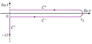
Figure 1: The L-shaped Kadanoff-Baym contour $\mathcal{C}=\mathcal{C}^{+}\cup\mathcal{C}^{-}\cup\mathcal{C}^{\circ}$, where the arrows indicate the contour ordering.

In the PI formalism, the multi-time impurity correlations can be naturally evaluated on a L-shaped contour, which can be seen as follows. Starting from the impurity-bath equilibrium state $e^{-\beta\hat{H}}$ with inverse temperature $\beta$, the impurity-bath state at time $t_{f}$ is

$$\hat{\rho}(t_{f})=e^{-{\rm i}\hat{H}t_{f}}e^{-\beta\hat{H}}e^{{\rm i}\hat{H}t_{f}}.$$ (4)

The impurity partition function at time $t_{f}$ is defined as

$$Z_{{\rm imp}}(t_{f}) \stackrel{{\scriptstyle\mathrm{def}}}{{=}}Z_{\mathrm{bath}}^{-1}\Tr\hat{\rho}(t_{f})$$

$$=Z_{\mathrm{bath}}^{-1}\Tr[e^{-\beta\hat{H}}e^{{\rm i}\hat{H}t_{f}}e^{-{\rm i}\hat{H}t_{f}}],$$ (5)

where $Z_{\mathrm{bath}}$ is the free bath partition function, and we have used the cyclic property of the trace in the second line. If we read the term inside the square bracket in the second line of Eq.(II.2) from right to left, we can think of the evolution as along such a contour: it starts from time $0$ to $t_{f}$ by a forward evolution $e^{-{\rm i}\hat{H}t_{f}}$, then it returns back to time 0 by a backward evolution $e^{{\rm i}\hat{H}t_{f}}$, and finally it goes to $-{\rm i}\beta$ by an imaginary time evolution $e^{-\beta\hat{H}}$. The whole contour, denoted as $\mathcal{C}$ in this work, is usually referred as Kadanoff-Baym contour [67, 5]. $\mathcal{C}$ consists of three branches: the forward branch $\mathcal{C}^{+}:0\to t_{f}$, the backward branch $\mathcal{C}^{-}:t_{f}\to 0$, and the imaginary branch $\mathcal{C}^{\circ}:0\to-{\rm i}\beta$, as shown in Fig. 1.

The PI for Eq.(II.2) can be formally written as

$$Z_{{\rm imp}}=\int\mathcal{D}[\bar{\bm{a}},\bm{a}]\mathcal{K}\left[\bar{\bm{a}},\bm{a}\right]\prod_{\sigma}\mathcal{I}_{\sigma}\left[\bar{\bm{a}}_{\sigma},\bm{a}_{\sigma}\right],$$ (6)

where $\bar{\bm{a}}_{\sigma}=\{\bar{a}_{\sigma}(t)\}$, $\bm{a}_{\sigma}=\{a_{\sigma}(t)\}$ are Grassmann trajectories on the Kadanoff-Baym contour, and $\bar{\bm{a}}=\{\bar{\bm{a}}_{\uparrow},\bar{\bm{a}}_{\downarrow}\},\bm{a}=\{\bm{a}_{\uparrow},\bm{a}_{\downarrow}\}$ for briefness. The measure is

$$\mathcal{D}[\bar{\bm{a}},\bm{a}]=\prod_{\sigma,t}\differential{\bar{a}_{\sigma}(t)}\differential{a_{\sigma}(t)}e^{-\bar{a}_{\sigma}(t)a_{\sigma}(t)}.$$ (7)

$\mathcal{K}$ is only determined by $\hat{H}_{\rm imp}$, which can be formally written as

$$\mathcal{K}\left[\bar{\bm{a}},\bm{a}\right]=e^{-{\rm i}\int_{\mathcal{C}}dt\mathcal{H}_{\rm imp}(t)}.$$ (8)

Here $\mathcal{H}_{\rm imp}$ is obtained from $\hat{H}_{\rm imp}$ by making the substitutions $\hat{a}(t)\to a(t)$, $\hat{a}^{\dagger}(t)\to\bar{a}(t)$, $dt$ should be understood as branch-dependent, that is, $dt=\pm\delta t$ on $\mathcal{C}^{\pm}$, and $dt=-{\rm i}\delta\tau$ on $\mathcal{C}^{\circ}$, where $\delta t$ and $\delta\tau$ are the time step size on the real-time and imaginary-time axes respectively. $\mathcal{I}_{\sigma}$ is determined by $\hat{H}_{\rm int}$ (more concretely, $J(\varepsilon)$), which can be formally written as

$$\mathcal{I}_{\sigma}[\bar{\bm{a}}_{\sigma},\bm{a}]=e^{-\int_{\mathcal{C}}dt\int_{\mathcal{C}}dt^{\prime}\bar{a}_{\sigma}(t)\Delta(t,t^{\prime})a_{\sigma}(t^{\prime})}.$$ (9)

$\Delta(t,t^{\prime})$ is the hybridization function which encodes all the bath effects and can be calculated by

$$\Delta(t,t^{\prime})={\rm i}\int\differential{\varepsilon}J(\varepsilon)D_{\varepsilon}(t,t^{\prime}).$$ (10)

with $D_{\varepsilon}(t,t^{\prime})$ the free bath contour-ordered Green’s function defined as

$$D_{\varepsilon}(t,t^{\prime})\stackrel{{\scriptstyle\mathrm{def}}}{{=}}-{\rm i}\expectationvalue*{T_{\mathcal{C}}\hat{c}_{\varepsilon}(t)\hat{c}^{\dagger}_{\varepsilon}(t^{\prime})}_{\mathrm{bath}}.$$ (11)

Here $T_{\mathcal{C}}$ is the contour-ordering operator that arranges operators on the contour in the order indicated by the arrows in Fig. 1, and $\expectationvalue{\cdots}_{\mathrm{bath}}$ means the expectation value with respect to the free bath.

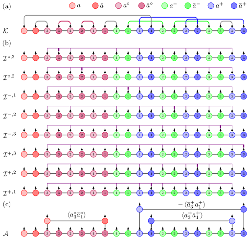
Figure 2: Schematic illustration of the construction of (a) $\mathcal{K}$ and (b) each partial influence functional as Grassmann MPSs for the non-interacting Toulouse model with $M=N=2$, such that only a single spin needs to be considered and the spin indices are omitted. The purple, green, blue solid circles with numbers represent Grassmann variables at different time steps on the imaginary, backward and forward branches respectively. The pair of red solid circles at the left boundary without numbers represent the additional pair of GVs introduced to take care of the boundary condition in the impurity path integral. In panel (b) we have shown the concrete patterns of all the $M+2(N+1)=8$ partial IFs, which are multiplied together to obtain $\mathcal{I}$ as a GMPS. (c) Calculating the Matsubara Green’s function $\mathcal{G}_{3,1}$, the greater Green’s function $G^{>}_{3,1}$ and the lesser Green’s function $G^{<}_{3,1}$ based on the augmented density tensor $\mathcal{A}$, corresponding to Eq.(18), Eq.(19) and Eq.(20) respectively.

II.3 The mixed-time GTEMPO method

The continuous expressions in Eq.(8) and Eq.(9) are more of notational convenience. In actual calculation, the continuous integral along $\mathcal{C}$ should be understood in the discrete sense where $\mathcal{C}$ is first broken into small finite pieces, and then one sums over the contributions from all the possible discrete paths formed by these pieces. In the following, we introduce in detail the discretization scheme we have used in our numerical implementation, which is in the same spirit as our implementations of the real-time [58] and imaginary-time [63] GTEMPO methods.

We denote $N=t/\delta t$, $M=\beta/\delta\tau$ as the total numbers of discrete time steps on the real- and imaginary-time axes respectively. We first discretize the continuous Grassmann trajectories into discrete ones as $\bar{\bm{a}}_{\sigma}^{\pm}=\{\bar{a}_{\sigma,N+1}^{\pm},\cdots,\bar{a}_{\sigma,1}^{\pm}\}$, $\bm{a}_{\sigma}^{\pm}=\{a_{\sigma,N+1}^{\pm},\cdots,a_{\sigma,1}^{\pm}\}$, $\bar{\bm{a}}_{\sigma}^{\circ}=\{\bar{a}_{\sigma,M+1}^{\circ},\cdots,\bar{a}_{\sigma,1}^{\circ}\}$ and $\bm{a}_{\sigma}^{\circ}=\{a_{\sigma,M+1}^{\circ},\cdots,a_{\sigma,1}^{\circ}\}$, where $a_{\sigma,j}^{\zeta}$ and $\bar{a}_{\sigma,j}^{\zeta}$ are a pair of conjugate Grassmann variables (GVs) at time step $j$ on $\mathcal{C}^{\zeta}$. We will also use $\bar{\bm{a}}_{j}^{\zeta}=\{\bar{a}_{\uparrow,j}^{\zeta},\bar{a}_{\downarrow,j}^{\zeta}\}$ and $\bm{a}_{j}^{\zeta}=\{a_{\uparrow,j}^{\zeta},a_{\downarrow,j}^{\zeta}\}$ to denote the set of GVs for both spins at the same time step $j$. In addition, we introduce a pair of GVs $a_{\sigma}$ and $\bar{a}_{\sigma}$ to account for the boundary condition [63], which corresponds to the final trace in Eq.(II.2). As a result, there will be $L=8(N+1)+4(M+1)+4$ GVs in total for the single-orbital AIM, which will also be the size of all the GMPSs involved in the mixed-time GTEMPO calculations. In our numerical implementation, those GVs are ordered as

$$a_{\uparrow}\bar{a}_{\uparrow}a_{\downarrow}\bar{a}_{\downarrow}a^{\circ}_{\uparrow,M+1}\bar{a}^{\circ}_{\uparrow,M+1}a^{\circ}_{\downarrow,M+1}\bar{a}^{\circ}_{\downarrow,M+1}\cdots a^{\circ}_{\uparrow,1}\bar{a}^{\circ}_{\uparrow,1}a^{\circ}_{\downarrow,1}\bar{a}^{\circ}_{\downarrow,1}$$

$$a^{-}_{\uparrow,1}\bar{a}^{-}_{\uparrow,1}a^{-}_{\downarrow,1}\bar{a}^{-}_{\downarrow,1}a^{+}_{\uparrow,1}\bar{a}^{+}_{\uparrow,1}a^{+}_{\downarrow,1}\bar{a}^{+}_{\downarrow,1}\cdots a^{-}_{\uparrow,N+1}\bar{a}^{-}_{\uparrow,N+1}$$

$$a^{-}_{\downarrow,N+1}\bar{a}^{-}_{\downarrow,N+1}a^{+}_{\uparrow,N+1}\bar{a}^{+}_{\uparrow,N+1}a^{+}_{\downarrow,N+1}\bar{a}^{+}_{\downarrow,N+1},$$ (12)

where we have arranged the $\pm$ branches in nearly positions, different from the original time order in Fig. 1.

Based on the above notations, the discretized expression for $\mathcal{K}$ can be written as

$$\mathcal{K}[\bar{\bm{a}},\bm{a}]= \innerproduct{-\bm{a}}{\bm{a}_{M+1}^{\circ}}\matrixelement{\bm{a}_{M+1}^{\circ}}{\hat{U}_{\rm imp}^{\circ}}{\bm{a}_{M}^{\circ}}\cdots\matrixelement{\bm{a}_{2}^{\circ}}{\hat{U}_{\rm imp}^{\circ}}{\bm{a}_{1}^{\circ}}$$

$$\times\innerproduct{\bm{a}_{1}^{\circ}}{a_{1}^{-}}\matrixelement{\bm{a}_{1}^{-}}{\hat{U}_{\rm imp}^{-}}{\bm{a}_{2}^{-}}\cdots\matrixelement{\bm{a}_{N}^{-}}{\hat{U}_{\rm imp}^{-}}{\bm{a}_{N+1}^{-}}$$

$$\times\innerproduct{\bm{a}_{N+1}^{-}}{\bm{a}_{N+1}^{+}}\matrixelement{\bm{a}_{N+1}^{+}}{\hat{U}_{\rm imp}^{+}}{\bm{a}_{N}^{+}}\cdots$$

$$\times\matrixelement{\bm{a}_{2}^{+}}{\hat{U}_{\rm imp}^{+}}{\bm{a}_{1}^{+}}\innerproduct{\bm{a}_{1}^{+}}{\bm{a}},$$ (13)

where $\bm{a}=\{a_{\uparrow},a_{\downarrow}\}$, $\bar{\bm{a}}=\{\bar{a}_{\uparrow},\bar{a}_{\downarrow}\}$ (the first and last term on the rhs take care of the boundary condition), and the discrete propagator $\hat{U}_{\rm imp}^{\zeta}=e^{-{\rm i}\hat{H}_{\rm imp}dt}$ (noticing that $dt$ is branch-dependent). For single-orbital AIM, the propagators can be exactly evaluated as:

$$\matrixelement{\bm{\xi}}{\hat{U}_{\rm imp}^{\zeta}}{\bm{\xi}^{\prime}} =e^{g^{\zeta}\sum_{\sigma}\bar{\xi}_{\sigma}\xi^{\prime}_{\sigma}+(g^{\zeta})^{2}(e^{-{\rm i}dtU}-1)\bar{\xi}_{\uparrow}\bar{\xi}_{\downarrow}\xi^{\prime}_{\downarrow}\xi^{\prime}_{\uparrow}}$$ (14)

with $g^{\zeta}=e^{-{\rm i}dt(\varepsilon_{d}-U/2)}$ [58, 63]. With the ordering of GVs in Eq.(II.3), $\mathcal{K}$ can be exactly built as a GMPS with bond dimension $16$. For more sophisticated impurity models, one could also easily adapt the algorithm proposed in Ref. [63] to obtain a numerically exact expression for $\mathcal{K}$.

The IF can be discretized using the quasi-adiabatic propagator path integral (QuaPI) method [68, 69], which results in a discrete expression in the form

$$\mathcal{I}_{\sigma}\approx e^{-\sum_{\zeta,\zeta^{\prime}}\sum_{jk}\bar{a}^{\zeta}_{\sigma,j}\Delta_{j,k}^{\zeta\zeta^{\prime}}a^{\zeta^{\prime}}_{\sigma,k}}.$$ (15)

There are $9$ hybridization matrices in total, and their expressions can be found in Appendix. A.

In this work, we build each $\mathcal{I}_{\sigma}$ as a GMPS using the partial-IF algorithm as described in Refs. [58, 61]. Concretely, we first rewrite Eq.(15) as

$$\mathcal{I}_{\sigma}\approx\prod_{\zeta,j}\mathcal{I}_{\sigma}^{\zeta,j}\stackrel{{\scriptstyle\mathrm{def}}}{{=}}\prod_{\zeta,j}\left(e^{-\sum_{\zeta^{\prime},k}\bar{a}^{\zeta}_{\sigma,j}\Delta_{j,k}^{\zeta\zeta^{\prime}}a^{\zeta^{\prime}}_{\sigma,k}}\right),$$ (16)

then each partial IF $\mathcal{I}_{\sigma}^{\zeta,j}$ can be exactly written as a GMPS with bond dimension $2$ only [61]. As a result, we can build $\mathcal{I}_{\sigma}$ as a GMPS by multiplying $M+2(N+1)$ GMPSs, during which MPS bond truncation is performed to keep the bond dimension of the resulting GMPS to be within a given threshold $\chi$ [56, 60]. The cost of this construction roughly scales as $O[(M+2N)^{2}\chi^{3}]$ as a general feature of the partial-IF algorithm [61].

The procedures to build $\mathcal{K}$ and each partial IF as GMPSs are schematically shown in Fig. 2(a,b) respectively, specialized for the noninteracting case such that we only need to consider a single spin for briefness. For the single-orbital AIM the construction of $\mathcal{K}$ will contain $4$-body terms, while the partial IFs for the two spins have exactly the same patterns as in Fig. 2(b), but acting on different spins separately.

II.4 Calculating Green’s functions

Once $\mathcal{K}$ and $\mathcal{I}_{\sigma}$ are both built as GMPSs, their product gives the GMPS representation of the augmented density tensor (ADT):

$$\mathcal{A}[\bar{\bm{a}},\bm{a}]=\mathcal{K}[\bar{\bm{a}},\bm{a}]\prod_{\sigma}\mathcal{I}_{\sigma}[\bar{\bm{a}}_{\sigma},\bm{a}_{\sigma}],$$ (17)

which is the integrand in Eq.(6). The ADT contains the information of the impurity dynamics on the whole Kadanoff-Baym contour, based on which any multi-time impurity correlation functions can be calculated straightforwardly. For example, the Matsubara Green’s function $\mathcal{G}_{j,k}$ between two imaginary-time steps $j$, $k$ ($j>k$) can be calculated as

$$-\mathcal{G}_{j,k} \stackrel{{\scriptstyle\mathrm{def}}}{{=}}\expectationvalue*{\hat{a}_{\sigma,j}\hat{a}^{\dagger}_{\sigma,k}}=\frac{\int\mathcal{D}[\bar{\bm{a}},\bm{a}]a_{\sigma,j}^{\circ}\bar{a}_{\sigma,k}^{\circ}\mathcal{A}[\bar{\bm{a}},\bm{a}]}{Z_{{\rm imp}}},$$ (18)

the greater Green’s function $G^{>}_{j,k}$ and lesser Green’s function $G^{<}_{j,k}$ can be calculated as

$${\rm i}G^{>}_{j,k} \stackrel{{\scriptstyle\mathrm{def}}}{{=}}\expectationvalue*{\hat{a}_{\sigma,j}\hat{a}^{\dagger}_{\sigma,k}}=\frac{\int\mathcal{D}[\bar{\bm{a}},\bm{a}]a_{\sigma,j}^{+}\bar{a}_{\sigma,k}^{+}\mathcal{A}[\bar{\bm{a}},\bm{a}]}{Z_{{\rm imp}}};$$ (19)

$$-{\rm i}G^{<}_{j,k} \stackrel{{\scriptstyle\mathrm{def}}}{{=}}\expectationvalue*{\hat{a}^{\dagger}_{\sigma,k}\hat{a}_{\sigma,j}}=\frac{\int\mathcal{D}[\bar{\bm{a}},\bm{a}]\bar{a}_{\sigma,k}^{-}a_{\sigma,j}^{+}\mathcal{A}[\bar{\bm{a}},\bm{a}]}{Z_{{\rm imp}}}.$$ (20)

With $G^{>}_{j,k}$ and $G^{<}_{j,k}$ , the retarded Green’s function $G_{j,k}$ can also be easily obtained from its definition

$$G_{j,k}\stackrel{{\scriptstyle\mathrm{def}}}{{=}}G^{>}_{j,k}-G^{<}_{j,k}.$$ (21)

It should be noted here that in practice $\mathcal{A}$ is not built directly, but computed on the fly using a zipup algorithm for efficiency [58, 63].

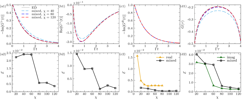
Figure 3: (a1, b1, c1, d1) The the imaginary (a1) and real (a2) parts of the greater Green’s function $G^{>}(t)$, the imaginary part of the retarded Green’s function $G(t)$ (c1), and Matsubara Green’s function $\mathcal{G}(\tau)$ of the Toulouse model as functions of the real (a1,b1,c1) or imaginary (d1) time. The gray solid lines are the ED results and the cyan, blue and red dashed lines are mixed-time GTEMPO results with bond dimension $\chi=40,80,120$ respectively. (a2, b2, c2, d2) The black solid line with square show the average errors of between the mixed-time GTEMPO results and ED results in (a1,b1,c1,d1) as functions of the bond dimension $\chi$. The yellow solid line with triangle in panel (c2) shows the average error between the real-time GTEMPO results and ED results, and the green solid line with triangle in panel (d2) shows the average error between the imaginary-time GTEMPO results and ED results. In these simulations we have used $\Gamma\delta t=0.005$ and $\Gamma\delta\tau=0.01$ for mixed-time GTEMPO, $\Gamma\delta t=0.005$ for real-time GTEMPO, and $\Gamma\delta\tau=0.01$ for imaginary-time GTEMPO.

III Numerical results

In the following we demonstrate the performance of the mixed-time GTEMPO method in the noninteracting case and in the single-orbital AIM. In our numerical simulations for this work we will focus on a semi-circular bath spectrum density

$$J(\varepsilon)=\frac{\Gamma D}{2\pi}\sqrt{1-(\varepsilon/D)^{2}},$$ (22)

with $D=2$ and $\Gamma=0.1$, and we will take $\Gamma$ as the unit.

We first validate the mixed-time GTEMPO method on the equilibrium Green’s functions in the noninteracting Toulouse model [70, 1], where we focus on the half filling case with $\epsilon_{d}=0$. In Fig. 3(a1, b1, c1, d1), we benchmark the imaginary and real parts of $G^{>}(t)$ ($G^{<}(t)$ has the same real part as and the opposite imaginary part to $G^{>}(t)$ for half filling, thus it is not shown), the imaginary part of $G(t)$ (the real part vanishes for half filling and is not shown), and $\mathcal{G}(\tau)$, calculated by mixed-time GTEMPO using different bond dimensions $\chi=40,80,120$ (the dashed lines), against the exact diagonalization (ED) results (the gray solid lines). For ED we have discretized the bath into $2000$ equal-distant frequencies ($\delta\varepsilon/\Gamma=0.005$) and we have verified that the ED results have well converged against bath discretization (which is the only error in ED). In Fig. 3(a2, b2, c2, d2), we show the average errors between the mixed-time GTEMPO results and ED results as a function of $\chi$, where the average error is defined as

$$\mathcal{E}(\vec{x},\vec{y})=\sqrt{\frac{||\vec{x}-\vec{y}||^{2}}{L}}$$ (23)

for two vectors $\vec{x}$ and $\vec{y}$ of length $L$. We can see that with $\chi=80$ both $G^{>}(t)$ and $\mathcal{G}(\tau)$ calculated by mixed-time GTEMPO already converges quite well with ED, with the average error within $1\%$. From Fig. 3(c1, c2), we can see that the retarded Green’s function, calculated from Eq.(21), converges much faster than $G^{>}(t)$, which means that the errors in $G^{>}(t)$ and $G^{<}(t)$ perfectly cancel each other even with a very small bond dimension $\chi=20$ (this cancellation is much better than in the real-time GTEMPO calculations shown by the yellow solid line with triangle), this is likely due to a coincidence that the noninteracting retarded Green’s function is independent of the initial state [1]. The dependence of the average error in the Matsubara Green’s function on $\chi$ is comparable to the imaginary-time GTEMPO calculations. Crucially, even though in the mixed-time GTEMPO calculations we deal with more GVs compared to the real- and imaginary-time GTEMPO calculations, we observe that the bond dimension required to obtain converged and accurate results seem to be not larger than the latter ones, thus the mixed-time GTEMPO calculation will not be a lot more expensive than the imaginary-time calculation (it has been observed that the imaginary-time GTEMPO calculations usually require larger bond dimensions than the real-time GTEMPO calculations to achieve similar accuracy [60]), as the computational cost of the partial-IF algorithm roughly scales quadratically with the number of GVs, and cubically with $\chi$ [61].

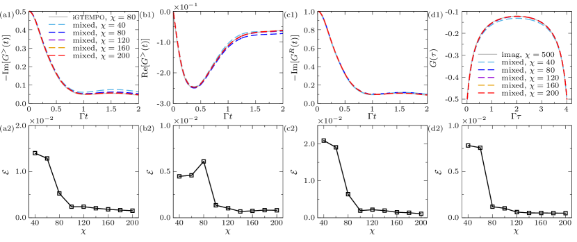
Figure 4: (a1, b1, c1, d1) The the imaginary (a1) and real (a2) parts of the greater Green’s function $G^{>}(t)$, the imaginary part of the retarded Green’s function $G(t)$ (c1), and Matsubara Green’s function $\mathcal{G}(\tau)$ of the single-orbital Anderson impurity model as functions of the real (a1,b1,c1) or imaginary (d1) time. The gray solid lines in (a1,b1,c1) are the infinite-time GTEMPO results calculated using $\chi=80$ and $\Gamma\delta t=0.005$. The gray solid line in (d1) is the imaginary-time GTEMPO results calculated with $\chi=500$ and $\Gamma\delta\tau=0.01$. (a2, b2, c2) The black solid line with square show the average errors between the mixed-time GTEMPO results and the baseline infinite-time GTEMPO results in (a1,b1,c1) against $\chi$. (d2) The black solid line with square show the average errors between the mixed-time GTEMPO results and the baseline imaginary-time GTEMPO results in (d1) against $\chi$. In these mixed-time GTEMPO calculations we have used $U/\Gamma=5$, $\Gamma\delta t=0.005$ and $\Gamma\delta\tau=0.01$.

Next we proceed to study the single-orbital AIM, and we still focus on the half-filling case with $U/\Gamma=-2\epsilon_{d}/\Gamma=5$. In this case there does not exist exact solutions. Nevertheless, for the Matsubara Green’s function we can benchmark the accuracy against imaginary-time GTEMPO calculations, and for real-time Green’s functions we can benchmark the accuracy against the infinite-time GTEMPO (referred to as iGTEMPO) calculations in Ref. [66] which directly aims at the steady state. Similar to Fig. 3, we show the imaginary and real parts of $G^{>}(t)$, the imaginary part of $G(t)$, and $\mathcal{G}(\tau)$ in Fig. 4(a1, b1, c1, d1) respectively. The gray solid lines in Fig. 4(a1,b1,c1) are the infinite-time GTEMPO results calculated with $\chi=80$ and $\Gamma\delta t=0.005$, which are also used as the baseline to calculate the average errors in Fig. 4(a2,b2,c2). The gray solid line in Fig. 4(d1) shows the imaginary-time GTEMPO results calculated with $\chi=500$ and $\Gamma\delta\tau=0.01$, which is also used as the baseline to calculate the average errors in Fig. 4(d2). Again we can see that $G^{>}(t)$ calculated by mixed-time GTEMPO using $\chi=80$ already agrees well with the iGTEMPO calculations, with average error within $1\%$. Meanwhile, the average error in $G^{>}(t)$ keeps decreasing with $\chi$, and only approximately converges at $\chi=200$. For $\mathcal{G}(\tau)$, the results calculated by mixed-time GTEMPO agree very well with the imaginary-time GTEMPO calculations at $\chi=80$ (the average error is $0.1\%$, which is about one order of magnitude smaller than the noninteracting case), which agrees with the previous observation that the imaginary-time GTEMPO calculations become more accurate for larger $U$ [63]. From Fig. 3(c1, c2), we can see that the behavior of the retarded Green’s function in the interacting case is similar to $G^{>}(t)$, in contrast with the noninteracting case.

IV Discussions

In summary, we have proposed a mixed-time GTEMPO method that works on the L-shaped Kadanoff-Baym contour. The method complements the previous iGTEMPO and imaginary-time GTEMPO methods, which allows to directly consider correlated impurity-bath initial state. It contains only three hyperparameters, the real-time step size $\delta t$ and imaginary-time step size $\delta\tau$, plus the MPS bond dimension $\chi$, which can all be well-controlled. In our numerical examples, we benchmark this method against exact solutions in the noninteracting case, and against the iGTEMPO and imaginary-time GTEMPO calculations in the single-orbital Anderson impurity model. Crucially, we observe that the bond dimension required in the mixed-time GTEMPO calculations is not larger than that required in the imaginary-time calculations, even though the size of the GMPS and the number of GMPS multiplications become larger, therefore the computational overhead of the mixed-time GTEMPO method will not be significant compared to the imaginary-time GTEMPO method. Compared to the iGTEMPO method, the mixed-time GTEMPO method will be less efficient, but it contains less hyperparameters than the latter. To our knowledge this is the first work which directly performs numerical calculations on Kadanoff-Baym contour for the Anderson impurity model. Since the errors in this method can be well-controlled, it is a perfect benchmarking baseline for more efficient alternatives but with less well-controlled approximations. It can also be used as an impurity solver in DMFT and non-equilibrium DMFT, where one can obtain the real- and imaginary-time Green’s functions simultaneously.

Appendix A Quasi-adiabatic propagator path integral on the Kadanoff-Baym contour

Here we list the explicit expressions of the $9$ hybridization matrices used in our numerical simulations. We use $n(\varepsilon)=(e^{\beta\varepsilon}+1)^{-1}$ to denoted the Fermi-Dirac distribution function.

$$\Delta_{j,k}^{++}=\begin{cases}\displaystyle 2\int d\varepsilon\frac{J(\varepsilon)}{\varepsilon^{2}}[1-n(\varepsilon)]e^{-{\rm i}\varepsilon(j-k)\delta t}(1-\cos\varepsilon\delta t),&j>k;\\ \displaystyle-2\int d\varepsilon\frac{J(\varepsilon)}{\varepsilon^{2}}n(\varepsilon)e^{-{\rm i}\varepsilon(j-k)\delta t}(1-\cos\varepsilon\delta t),&j<k;\\ \displaystyle\int d\varepsilon\frac{J(\varepsilon)}{\varepsilon^{2}}\quantity{[1-n(\varepsilon)][(1-{\rm i}\varepsilon\delta t)-e^{-{\rm i}\varepsilon\delta t}]-n(\varepsilon)[(1+{\rm i}\varepsilon\delta t)-e^{{\rm i}\varepsilon\delta t}]},&j=k,\end{cases}$$ (24)

$$\Delta^{+-}_{j,k}=\displaystyle 2\int d\varepsilon\frac{J(\varepsilon)}{\varepsilon^{2}}n(\varepsilon)e^{-{\rm i}\varepsilon(j-k)\delta t}(1-\cos\varepsilon\delta t),$$ (25)

$$\Delta^{+\circ}_{j,k}=-\int d\varepsilon\frac{J(\varepsilon)}{\varepsilon^{2}}n(\varepsilon)e^{-{\rm i}\varepsilon j\delta t}e^{\varepsilon k\delta\tau}(e^{-{\rm i}\varepsilon\delta t}-1)(e^{\varepsilon\delta\tau}-1),$$ (26)

$$\Delta^{-+}_{j,k}=\displaystyle-2\int d\varepsilon\frac{J(\varepsilon)}{\varepsilon^{2}}[1-n(\varepsilon)]e^{-{\rm i}\varepsilon(j-k)\delta t}(1-\cos\varepsilon\delta t),$$ (27)

$$\Delta^{--}_{j,k}=\begin{cases}\displaystyle-2\int d\varepsilon\frac{J(\varepsilon)}{\varepsilon^{2}}n(\varepsilon)e^{-{\rm i}\varepsilon(j-k)\delta t}(1-\cos\varepsilon\delta t),&j>k;\\ \displaystyle 2\int d\varepsilon\frac{J(\varepsilon)}{\varepsilon^{2}}[1-n(\varepsilon)]e^{-{\rm i}\varepsilon(j-k)\delta t}(1-\cos\varepsilon\delta t),&j<k;\\ \displaystyle-\int d\varepsilon\frac{J(\varepsilon)}{\varepsilon^{2}}\quantity{n(\varepsilon)[(1-{\rm i}\varepsilon\delta t)-e^{-{\rm i}\varepsilon\delta t}]-[1-n(\varepsilon)][(1+{\rm i}\varepsilon\delta t)-e^{{\rm i}\varepsilon\delta t}]},&j=k,\end{cases}$$ (28)

$$\Delta^{-\circ}_{j,k}=\int d\varepsilon\frac{J(\varepsilon)}{\varepsilon^{2}}n(\varepsilon)e^{-{\rm i}\varepsilon j\delta t}e^{\varepsilon k\delta\tau}(e^{-{\rm i}\varepsilon\delta t}-1)(e^{\varepsilon\delta\tau}-1),$$ (29)

$$\Delta^{\circ+}_{j,k}=\int d\varepsilon\frac{J(\varepsilon)}{\varepsilon^{2}}[1-n(\varepsilon)]e^{-\varepsilon j\delta\tau}e^{{\rm i}\varepsilon k\delta t}(e^{{\rm i}\varepsilon\delta t}-1)(e^{-\varepsilon\delta\tau}-1),$$ (30)

$$\Delta^{\circ-}_{j,k}=-\int d\varepsilon\frac{J(\varepsilon)}{\varepsilon^{2}}[1-n(\varepsilon)]e^{-\varepsilon j\delta\tau}e^{{\rm i}\varepsilon k\delta t}(e^{{\rm i}\varepsilon\delta t}-1)(e^{-\varepsilon\delta\tau}-1),$$ (31)

$$\Delta^{\circ\circ}_{j,k}=\begin{cases}\displaystyle-2\int d\varepsilon\frac{J(\varepsilon)}{\varepsilon^{2}}[1-n(\varepsilon)]e^{-\varepsilon(j-k)\delta\tau}(1-\cosh\varepsilon\delta\tau),&j>k;\\ \displaystyle 2\int d\varepsilon\frac{J(\varepsilon)}{\varepsilon^{2}}n(\varepsilon)e^{-\varepsilon(j-k)\delta\tau}(1-\cosh\varepsilon\delta\tau),&j<k;\\ \displaystyle-\int d\varepsilon\frac{J(\varepsilon)}{\varepsilon^{2}}\quantity{[1-n(\varepsilon)][(1-\varepsilon\delta\tau)-e^{-\varepsilon\delta\tau}]-n(\varepsilon)[(1+\varepsilon\delta\tau)-e^{\varepsilon\delta\tau}]},&j=k.\end{cases}$$ (32)

References

- Mahan [2000] G. D. Mahan, Many-Particle Physics (Springer; 3nd edition, 2000).
- Weiss [1993] U. Weiss, Quantum Dissipative Systems (World Scientific, Singapore, 1993).
- Georges et al. [1996] A. Georges, G. Kotliar, W. Krauth, and M. J. Rozenberg, Dynamical mean-field theory of strongly correlated fermion systems and the limit of infinite dimensions, Rev. Mod. Phys. 68, 13 (1996).
- Gull et al. [2011] E. Gull, A. J. Millis, A. I. Lichtenstein, A. N. Rubtsov, M. Troyer, and P. Werner, Continuous-time monte carlo methods for quantum impurity models, Rev. Mod. Phys. 83, 349 (2011).
- Aoki et al. [2014] H. Aoki, N. Tsuji, M. Eckstein, M. Kollar, T. Oka, and P. Werner, Nonequilibrium dynamical mean-field theory and its applications, Rev. Mod. Phys. 86, 779 (2014).
- Caffarel and Krauth [1994] M. Caffarel and W. Krauth, Exact diagonalization approach to correlated fermions in infinite dimensions: Mott transition and superconductivity, Phys. Rev. Lett. 72, 1545 (1994).
- Koch et al. [2008] E. Koch, G. Sangiovanni, and O. Gunnarsson, Sum rules and bath parametrization for quantum cluster theories, Phys. Rev. B 78, 115102 (2008).
- Granath and Strand [2012] M. Granath and H. U. R. Strand, Distributional exact diagonalization formalism for quantum impurity models, Phys. Rev. B 86, 115111 (2012).
- Lu et al. [2014] Y. Lu, M. Höppner, O. Gunnarsson, and M. W. Haverkort, Efficient real-frequency solver for dynamical mean-field theory, Phys. Rev. B 90, 085102 (2014).
- Mejuto-Zaera et al. [2020] C. Mejuto-Zaera, L. Zepeda-Núñez, M. Lindsey, N. Tubman, B. Whaley, and L. Lin, Efficient hybridization fitting for dynamical mean-field theory via semi-definite relaxation, Phys. Rev. B 101, 035143 (2020).
- He and Lu [2014] R.-Q. He and Z.-Y. Lu, Quantum renormalization groups based on natural orbitals, Phys. Rev. B 89, 085108 (2014).
- He et al. [2015] R.-Q. He, J. Dai, and Z.-Y. Lu, Natural orbitals renormalization group approach to the two-impurity kondo critical point, Phys. Rev. B 91, 155140 (2015).
- Wilson [1975] K. G. Wilson, The renormalization group: Critical phenomena and the kondo problem, Rev. Mod. Phys. 47, 773 (1975).
- Bulla [1999] R. Bulla, Zero temperature metal-insulator transition in the infinite-dimensional hubbard model, Phys. Rev. Lett. 83, 136 (1999).
- Bulla et al. [2008] R. Bulla, T. A. Costi, and T. Pruschke, Numerical renormalization group method for quantum impurity systems, Rev. Mod. Phys. 80, 395 (2008).
- Anders [2008] F. B. Anders, A numerical renormalization group approach to non-equilibrium green functions for quantum impurity models, J. Phys. Condens. Matter 20, 195216 (2008).
- Žitko and Pruschke [2009] R. Žitko and T. Pruschke, Energy resolution and discretization artifacts in the numerical renormalization group, Phys. Rev. B 79, 085106 (2009).
- Deng et al. [2013] X. Deng, J. Mravlje, R. Žitko, M. Ferrero, G. Kotliar, and A. Georges, How bad metals turn good: Spectroscopic signatures of resilient quasiparticles, Phys. Rev. Lett. 110, 086401 (2013).
- Stadler et al. [2015] K. M. Stadler, Z. P. Yin, J. von Delft, G. Kotliar, and A. Weichselbaum, Dynamical mean-field theory plus numerical renormalization-group study of spin-orbital separation in a three-band hund metal, Phys. Rev. Lett. 115, 136401 (2015).
- Lee and Weichselbaum [2016] S.-S. B. Lee and A. Weichselbaum, Adaptive broadening to improve spectral resolution in the numerical renormalization group, Phys. Rev. B 94, 235127 (2016).
- Lee et al. [2017] S.-S. B. Lee, J. von Delft, and A. Weichselbaum, Doublon-holon origin of the subpeaks at the hubbard band edges, Phys. Rev. Lett. 119, 236402 (2017).
- Wolf et al. [2014] F. A. Wolf, I. P. McCulloch, O. Parcollet, and U. Schollwöck, Chebyshev matrix product state impurity solver for dynamical mean-field theory, Phys. Rev. B 90, 115124 (2014).
- Ganahl et al. [2014] M. Ganahl, P. Thunström, F. Verstraete, K. Held, and H. G. Evertz, Chebyshev expansion for impurity models using matrix product states, Phys. Rev. B 90, 045144 (2014).
- Ganahl et al. [2015] M. Ganahl, M. Aichhorn, H. G. Evertz, P. Thunström, K. Held, and F. Verstraete, Efficient dmft impurity solver using real-time dynamics with matrix product states, Phys. Rev. B 92, 155132 (2015).
- Wolf et al. [2015] F. A. Wolf, A. Go, I. P. McCulloch, A. J. Millis, and U. Schollwöck, Imaginary-time matrix product state impurity solver for dynamical mean-field theory, Phys. Rev. X 5, 041032 (2015).
- García et al. [2004] D. J. García, K. Hallberg, and M. J. Rozenberg, Dynamical mean field theory with the density matrix renormalization group, Phys. Rev. Lett. 93, 246403 (2004).
- Nishimoto et al. [2006] S. Nishimoto, F. Gebhard, and E. Jeckelmann, Dynamical mean-field theory calculation with the dynamical density-matrix renormalization group, Physica B Condens. Matter 378-380, 283 (2006).
- Weichselbaum et al. [2009] A. Weichselbaum, F. Verstraete, U. Schollwöck, J. I. Cirac, and J. von Delft, Variational matrix-product-state approach to quantum impurity models, Phys. Rev. B 80, 165117 (2009).
- Bauernfeind et al. [2017] D. Bauernfeind, M. Zingl, R. Triebl, M. Aichhorn, and H. G. Evertz, Fork tensor-product states: Efficient multiorbital real-time dmft solver, Phys. Rev. X 7, 031013 (2017).
- Lu et al. [2019] Y. Lu, X. Cao, P. Hansmann, and M. W. Haverkort, Natural-orbital impurity solver and projection approach for green’s functions, Phys. Rev. B 100, 115134 (2019).
- Werner et al. [2023] D. Werner, J. Lotze, and E. Arrigoni, Configuration interaction based nonequilibrium steady state impurity solver, Phys. Rev. B 107, 075119 (2023).
- Kohn and Santoro [2021] L. Kohn and G. E. Santoro, Efficient mapping for anderson impurity problems with matrix product states, Phys. Rev. B 104, 014303 (2021).
- Kohn and Santoro [2022] L. Kohn and G. E. Santoro, Quench dynamics of the anderson impurity model at finite temperature using matrix product states: entanglement and bath dynamics, J. Stat. Mech. Theory Exp. 2022, 063102 (2022).
- Feynman and Vernon [1963] R. P. Feynman and F. L. Vernon, The theory of a general quantum system interacting with a linear dissipative system, Ann. Phys. 24, 118 (1963).
- Rubtsov et al. [2005] A. N. Rubtsov, V. V. Savkin, and A. I. Lichtenstein, Continuous-time quantum monte carlo method for fermions, Phys. Rev. B 72, 035122 (2005).
- Gull et al. [2008] E. Gull, P. Werner, O. Parcollet, and M. Troyer, Continuous-time auxiliary-field monte carlo for quantum impurity models, EPL 82, 57003 (2008).
- Werner and Millis [2006] P. Werner and A. J. Millis, Hybridization expansion impurity solver: General formulation and application to kondo lattice and two-orbital models, Phys. Rev. B 74, 155107 (2006).
- Werner et al. [2006] P. Werner, A. Comanac, L. de’ Medici, M. Troyer, and A. J. Millis, Continuous-time solver for quantum impurity models, Phys. Rev. Lett. 97, 076405 (2006).
- Shinaoka et al. [2017] H. Shinaoka, E. Gull, and P. Werner, Continuous-time hybridization expansion quantum impurity solver for multi-orbital systems with complex hybridizations, Comput. Phys. Commun. 215, 128 (2017).
- Eidelstein et al. [2020] E. Eidelstein, E. Gull, and G. Cohen, Multiorbital quantum impurity solver for general interactions and hybridizations, Phys. Rev. Lett. 124, 206405 (2020).
- Cohen et al. [2014a] G. Cohen, D. R. Reichman, A. J. Millis, and E. Gull, Green’s functions from real-time bold-line monte carlo, Phys. Rev. B 89, 115139 (2014a).
- Cohen et al. [2014b] G. Cohen, E. Gull, D. R. Reichman, and A. J. Millis, Green’s functions from real-time bold-line monte carlo calculations: Spectral properties of the nonequilibrium anderson impurity model, Phys. Rev. Lett. 112, 146802 (2014b).
- Cohen et al. [2015] G. Cohen, E. Gull, D. R. Reichman, and A. J. Millis, Taming the dynamical sign problem in real-time evolution of quantum many-body problems, Phys. Rev. Lett. 115, 266802 (2015).
- Chen et al. [2017a] H.-T. Chen, G. Cohen, and D. R. Reichman, Inchworm Monte Carlo for exact non-adiabatic dynamics. I. Theory and algorithms, J. Chem. Phys. 146, 054105 (2017a).
- Chen et al. [2017b] H.-T. Chen, G. Cohen, and D. R. Reichman, Inchworm Monte Carlo for exact non-adiabatic dynamics. II. Benchmarks and comparison with established methods, J. Chem. Phys. 146, 054106 (2017b).
- Erpenbeck et al. [2023] A. Erpenbeck, E. Gull, and G. Cohen, Quantum monte carlo method in the steady state, Phys. Rev. Lett. 130, 186301 (2023).
- Tanimura and Kubo [1989] Y. Tanimura and R. Kubo, Time evolution of a quantum system in contact with a nearly gaussian-markoffian noise bath, J. Phys. Soc. Jpn. 58, 101 (1989).
- Jin et al. [2007] J. Jin, S. Welack, J. Luo, X.-Q. Li, P. Cui, R.-X. Xu, and Y. Yan, Dynamics of quantum dissipation systems interacting with fermion and boson grand canonical bath ensembles: Hierarchical equations of motion approach, J. Chem. Phys. 126, 134113 (2007).
- Jin et al. [2008] J. Jin, X. Zheng, and Y. Yan, Exact dynamics of dissipative electronic systems and quantum transport: Hierarchical equations of motion approach, J. Chem. Phys. 128, 234703 (2008).
- Yan et al. [2016] Y. Yan, J. Jin, R.-X. Xu, and X. Zheng, Dissipation equation of motion approach to open quantum systems, Front. Phys. 11, 110306 (2016).
- Cao et al. [2023] J. Cao, L. Ye, R. Xu, X. Zheng, and Y. Yan, Recent advances in fermionic hierarchical equations of motion method for strongly correlated quantum impurity systems, JUSTC 53, 0302 (2023).
- Tanimura [2014] Y. Tanimura, Reduced hierarchical equations of motion in real and imaginary time: Correlated initial states and thermodynamic quantities, J. Chem. Phys. 141, 044114 (2014).
- Xing et al. [2022] T. Xing, T. Li, Y. Yan, S. Bai, and Q. Shi, Application of the imaginary time hierarchical equations of motion method to calculate real time correlation functions, J. Chem. Phys. 156, 244102 (2022).
- Shao and Makri [2002] J. Shao and N. Makri, Iterative path integral formulation of equilibrium correlation functions for quantum dissipative systems, J. Chem. Phys. 116, 507 (2002).
- Thoenniss et al. [2023a] J. Thoenniss, A. Lerose, and D. A. Abanin, Nonequilibrium quantum impurity problems via matrix-product states in the temporal domain, Phys. Rev. B 107, 195101 (2023a).
- Thoenniss et al. [2023b] J. Thoenniss, M. Sonner, A. Lerose, and D. A. Abanin, Efficient method for quantum impurity problems out of equilibrium, Phys. Rev. B 107, L201115 (2023b).
- Ng et al. [2023] N. Ng, G. Park, A. J. Millis, G. K.-L. Chan, and D. R. Reichman, Real-time evolution of anderson impurity models via tensor network influence functionals, Phys. Rev. B 107, 125103 (2023).
- Chen et al. [2024a] R. Chen, X. Xu, and C. Guo, Grassmann time-evolving matrix product operators for quantum impurity models, Phys. Rev. B 109, 045140 (2024a).
- Strathearn et al. [2018] A. Strathearn, P. Kirton, D. Kilda, J. Keeling, and B. W. Lovett, Efficient non-markovian quantum dynamics using time-evolving matrix product operators, Nat. Commun. 9, 3322 (2018).
- Chen et al. [2024b] R. Chen, X. Xu, and C. Guo, Real-time impurity solver using grassmann time-evolving matrix product operators, Phys. Rev. B 109, 165113 (2024b).
- Guo and Chen [2024a] C. Guo and R. Chen, Efficient construction of the feynman-vernon influence functional as matrix product states, arXiv:2402.14350 (2024a).
- Kloss et al. [2023] B. Kloss, J. Thoenniss, M. Sonner, A. Lerose, M. T. Fishman, E. M. Stoudenmire, O. Parcollet, A. Georges, and D. A. Abanin, Equilibrium quantum impurity problems via matrix product state encoding of the retarded action, Phys. Rev. B 108, 205110 (2023).
- Chen et al. [2024c] R. Chen, X. Xu, and C. Guo, Grassmann time-evolving matrix product operators for equilibrium quantum impurity problems, New J. Phys. 26, 013019 (2024c).
- Jarrell and Biham [1989] M. Jarrell and O. Biham, Dynamical approach to analytic continuation of quantum monte carlo data, Phys. Rev. Lett. 63, 2504 (1989).
- Fei et al. [2021] J. Fei, C.-N. Yeh, and E. Gull, Nevanlinna analytical continuation, Phys. Rev. Lett. 126, 056402 (2021).
- Guo and Chen [2024b] C. Guo and R. Chen, Infinite grassmann time-evolving matrix product operator method in the steady state, arXiv:2403.16700 (2024b).
- Kadanoff and Baym [1962] L. P. Kadanoff and G. Baym, Quantum Statistical Mechnics (W. A. Benjamin, New York, 1962).
- Makarov and Makri [1994] D. E. Makarov and N. Makri, Path integrals for dissipative systems by tensor multiplication. condensed phase quantum dynamics for arbitrarily long time, Chem. Phys. Lett. 221, 482 (1994).
- Makri [1995] N. Makri, Numerical path integral techniques for long time dynamics of quantum dissipative systems, J. Math. Phys. 36, 2430 (1995).
- Leggett et al. [1987] A. J. Leggett, S. Chakravarty, A. T. Dorsey, M. P. A. Fisher, A. Garg, and W. Zwerger, Dynamics of the dissipative two-state system, Rev. Mod. Phys. 59, 1 (1987).