SoK: Gradient Leakage in Federated Learning

Abstract

Federated learning (FL) enables collaborative model training among multiple clients without raw data exposure. However, recent studies have shown that clients’ private training data can be reconstructed from the gradients they share in FL, known as gradient inversion attacks (GIAs). While GIAs have demonstrated effectiveness under ideal settings and auxiliary assumptions, their actual efficacy against practical FL systems remains under-explored. To address this gap, we conduct a comprehensive study on GIAs in this work. We start with a survey of GIAs that establishes a milestone to trace their evolution and develops a systematization to uncover their inherent threats. Specifically, we categorize the auxiliary assumptions used by existing GIAs based on their practical accessibility to potential adversaries. To facilitate deeper analysis, we highlight the challenges that GIAs face in practical FL systems from three perspectives: local training, model, and post-processing. We then perform extensive theoretical and empirical evaluations of state-of-the-art GIAs across diverse settings, utilizing eight datasets and thirteen models. Our findings indicate that GIAs have inherent limitations when reconstructing data under practical local training settings. Furthermore, their efficacy is sensitive to the trained model, and even simple post-processing measures applied to gradients can be effective defenses. Overall, our work provides crucial insights into the limited effectiveness of GIAs in practical FL systems. By rectifying prior misconceptions, we hope to inspire more accurate and realistic investigations on this topic.

1 Introduction

Federated learning (FL)[15] has recently become a widely adopted privacy-preserving distributed machine learning paradigm. In FL, multiple clients collaborate to train a global model orchestrated by a central server for multiple rounds. In each round, clients update the global model locally using private training data and then transmit gradients to the server for aggregation and global update, thereby alleviating privacy concerns from raw data exposure[16]. Therefore, FL has attracted considerable academic interests and empowered various real-world applications, including mobile services such as Google Keyboard[18] and Apple’s Siri[109], healthcare[111, 112], and finance[113, 114].

However, recent works claim that clients’ data privacy can be compromised by their gradient sharing in FL[20, 19]. Notably, a curious central server can reconstruct their private data by employing gradient inversion attacks (GIAs)[20]. Fig. 1 depicts the development and milestones of the GIA, presenting two forms:

$\bullet$ Optimization-based GIA: Initial GIAs assumed an honest-but-curious server and employed optimization-based methods to passively reconstruct the victim client’s training data [20, 19]. In this approach, the adversary (server) randomly initializes data and labels, computes gradients based on the same model as the victim client, and iteratively updates these initializations to mirror the ground truth by minimizing the dissimilarity between the computed gradient the the client’s shared gradient[19]. Subsequent advancements aimed to reconstruct larger-batch or higher-resolution data by assuming that the adversary not only possesses gradients but also auxiliary knowledge, such as Batch Normalization (BN) statistics [83] [3], client’s data distribution [4, 5, 9], etc. Accordingly, various regularization terms were devised, or Generative Adversarial Networks (GANs) [84] were leveraged to enhance GIA’s performance on more complicated tasks.

$\bullet$ Analytic-based GIA: Analytic-based methods aim to directly reconstruct training data by formulating and solving equations between gradients and inputs [30, 31]. Recent research efforts have extended this approach to handling inputs with higher dimensions, assuming a malicious server capable of actively crafting [33, 35] or modifying [34, 22, 36, 37] model parameters. Consequently, when a client inputs its private data into the malicious model, these inputs leave an “imprint” in the shared gradient, enabling the server to retrieve them by solving equations.

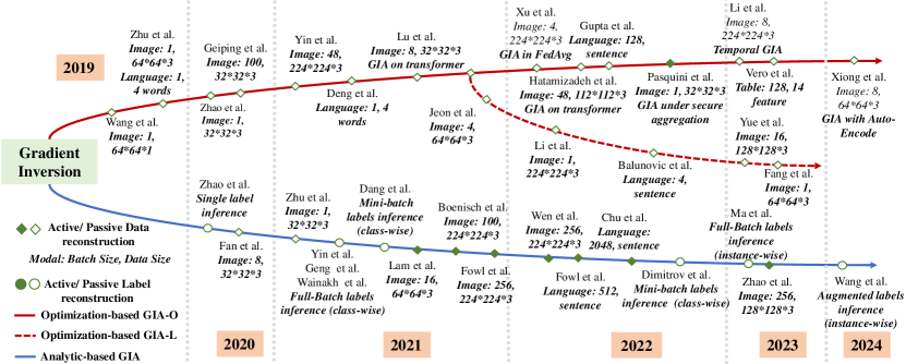
Figure 1: Development of Gradient Inversion Attack.

Despite the rapid growth and impressive performance of the GIA, there remains skepticism about its real capability and threat to practical FL systems, as often claimed. On one hand, existing works tend to obsess over employing auxiliary assumptions to achieve heightened performance. Reviewing the milestones, Yin et al. [3] assumed the adversary possesses additional access to BN statistics as side information, while Lam et al. [96] relaxed server assumptions to a malicious extent, allowing the adversary to impractically tamper with the model. On the other hand, these works often evaluate GIAs in settings far from practicality. For instance, literature frequently assumes a specific client who aggregates all private data into a single batch and undergoes a single step of model update, benefiting the adversary. However, in practical scenarios, gradients are typically uploaded after mini-batch Stochastic Gradient Descent (SGD) and multiple-epoch training [15]. Moreover, models generating gradients are often specially initialized [19] or designed [2, 3] solely to advantage the adversary and achieve superior reconstruction quality.

In this work, we conduct a comprehensive study on the GIA to better understand its nature and real threats to practical FL systems. Specifically, we make the following key contributions:

i@. A survey on GIA. We start by establishing a summary on the development of the GIA. To our knowledge, we are the first to thoroughly review the related works on the GIA, highlighting the milestones and breakthroughs in performance, as shown in Fig. 1. Moreover, we conduct a systematization of the GIA along three dimensions (Sec. 2): threat model, attack, and defense, as detailed in Appendix. Notably, we are the first to characterize the threat model of the GIA, categorizing the assumptions based on their practical accessibility to potential adversaries.

ii@. Rethinking GIA in practical FL. We examine the challenges GIA encounters in practical FL systems by comparing practice with literature from three crucial aspects that could influence GIA’s performance: local training, model, and post-processing (Sec. 3). Our discussion establishes a bridge between GIAs’ concepts in the literature and their practical implementations, leading us to derive six key research questions that further drive us to unveil the real threats posed by GIAs.

iii@. Analysis and insights for GIA in practical FL. We conduct comprehensive theoretical analyses and empirical evaluations on GIAs from the above-identified three aspects (in Sec. 4, Sec. 5, and Sec. 6, respectively) on 8 datasets and 13 models across diverse FL settings. Our findings reveal that despite GIAs’ claimed effectiveness, there exist inevitable bottlenecks and limitations. Contrary to expectations, they present minimal threat to practical FL systems, substantiated by the following observations:

(1) GIA has inevitable bottlenecks in data reconstruction against FL with practical local training. We investigate how the client’s local training impacts GIAs from two aspects, i.e., training configuration and training data. Specifically, we theoretically prove that as the number of local mini-batch SGD-based updates increases, reconstruction becomes much more difficult (Sec. 4.1). Moreover, we evaluate the capabilities of state-of-the-art GIAs in reconstructing data with wide ranges of batch sizes (ranging from 1 to 100) and resolutions (spanning from 32$\times$32 to 512$\times$512). Our analysis reveals the GIA’s bottleneck in reconstructing data as its dimensions grow (Sec. 4.2.1). Simultaneously, we are the first to identify that data content significantly affects GIAs. Specifically, GIA fails to guarantee the reconstruction of semantic details containing crucial private information. Additionally, we highlight that out-of-distribution (OOD) data significantly constrains GIA’s performance (Sec. 4.2.2) by introducing a novel OOD-test set.

(2) GIA is extremely sensitive to the model, including training stage and architecture. We propose a novel Input-Gradient Smoothness Analysis (IGSA) method to quantify and explain the model’s vulnerability to the GIA during the FL training process (Sec. 5.1). Surprisingly, our findings indicate that the GIA exclusively works in the early stages of training. Furthermore, we undertake the first investigation into the strong correlation between model architecture and the GIA. Our combined theoretical and empirical analyses highlight that commonly employed structures (such as skip connections[48] and Net-In-Net (NIN)[68]), and even seemingly insignificant micro designs (e.g., ReLU, kernel function size, etc.), significantly impact the model’s resilience against GIAs (Sec. 5.2).

(3) Even trivial post-processing measures applied to gradients in practical FL systems can effectively defend against GIAs while maintaining model accuracy. We evaluate four post-processing techniques, considering the privacy-utility trade-off within a practical FL setting. We show that even when confronted with state-of-the-art GIAs, clients can readily defend against them by employing post-processing strategies (e.g., quantization [77], sparsification [80]) to obscure the shared gradients (Sec. 6).

2 Systematization of Gradient Inversion

2.1 System Model

We consider an FL system consisting of a server and $M$ clients, each with a private training dataset containing $N$ data samples denoted by pairs of data ($x$) and labels ($y$). The $M$ clients collaboratively train a global model $W^{g}$ over $T$ rounds under the coordination of the server. In each round $t$, the server selects $K$ clients from the $M$ and sends the current global model $W^{g}_{t}$ to them for local training. Each client $k$ performs $E$ epochs of local training utilizing mini-batch SGD with a batch size of $B$. Consequently, each client performs $U=EN/B$ local updates. The diverse configurations of $E$ and $B$ give rise to two different local training protocols:

(1) FedSGD (Federated Stochastic Gradient Descent) [92]: Each client $k$ aggregates all $N$ local training data samples into a batch ($B=N$) and executes a single epoch of local training ($E=1$). As a result, the global model $W^{g}_{t}$ undergoes a sole update ($U=EN/B=1$). The computed gradient $\nabla_{k}W^{g}_{t}$ is uploaded to the server. The server aggregates the collected gradients and updates the global model as follows: $W^{g}_{t+1}\leftarrow W^{g}_{t}+\eta\sum_{k=1}^{K}\nabla_{k}W^{g}_{t}$.

(2) FedAvg (Federated Averaging) [15]: Client $k$ conducts $E>1$ epochs of mini-batch SGD with $B\leq N$ for local training and obtains an updated local model $W^{k}_{t+1}$. Unlike FedSGD, the server receives the $K$ local models and computes their average to obtain the updated global model: $W^{g}_{t+1}\leftarrow\frac{1}{K}\sum_{k=1}^{K}W^{k}_{t+1}$. In this scenario, the server lacks direct access to the gradient of client $k$. Instead, it acquires the model update through $W^{k}_{t+1}-W^{g}_{t}$, which also contains information regarding the training data. Throughout this paper, the term update is interchangeably used with gradient to ensure clarity and avoid ambiguity.

2.2 Threat Model

Existing studies primarily focus on scenarios where the server, receiving gradients from clients, acts as the adversary conducting GIAs. Following an extensive review of related literature, we discuss the prevailing threat model in existing GIAs based on the following three aspects:

(1) Goal. The goal of the adversary is to reconstruct the client’s data ($x$) and labels ($y$) that generate the shared gradient. Initial investigations into the GIA (e.g., [19]) aimed at reconstructing the data $x$ and labels $y$ from gradient simultaneously. Subsequent studies[23, 3] revealed the direct inference of labels from gradients. Consequently, the majority of GIA research focused on data reconstruction [3], given that data is the adversary’s primary target. Meanwhile, investigations such as [94, 28, 95] explored label inference, which has dual implications: First, foreknowledge of labels aids subsequent data reconstruction. Second, labels themselves contain sensitive information, revealing details such as a user’s purchase history (in online advertising) or their health status (in disease prediction)[97]. So far, GIAs have demonstrated capabilities to infer the existence of label classes (class-wise)[3] and the count of instances within each class (instance-wise)[95] from a full-batch[3, 27, 93, 95, 118] or multiple mini-batches[94, 28].

(2) Capacity & Server’s Trustworthiness. Most existing GIAs presume an honest-but-curious server[20, 19, 23, 2, 3, 30, 31, 27, 93, 85, 4, 94, 5, 6, 8, 9, 7, 28, 29, 29, 95, 86], which implies that the server merely analyzes shared gradients passively without interrupting the training process. Consequently, the victim client remains unaware, ensuring the stealthiness of GIAs. Furthermore, some studies consider that the server not only analyzes the gradient but could also actively interferes with the learning process through some malicious behaviors, thereby extracting more information about the input by the gradient. Specifically, they consider that the server can craft[32, 33, 35] or modify[34, 36, 37, 22] the model parameters, which enables the adversary to achieve better reconstruction results. It is worth noting that, unlike the honest-but-curious server, such malicious behaviors struggle to evade detection by the client.

(3) Assumption. Assumptions specifies the adversary’s knowledge and behaviors. Reflecting on the evolution of the GIA, diverse assumptions not only offer additional advantages to the adversary but also serve as key factors contributing to the asserted performances of certain GIAs[26]. Herein, we categorize and rank existing assumptions based on their accessibility to the adversary within practical FL systems and assign them to each work in Appendix.

[Level $0$]: Basic information refers to the necessities for gradient inversion, including gradient, model, data dimension, and number of data samples $N$ at clients, which are readily accessible to the server in practical FL systems.

[Level $1$]: Priors refer to side information, including established data patterns or observations on gradients that are readily accessible. For instance, Geiping et al. in[2] utilized total variation [25] as a prior, reflecting an established pattern of smoothness among neighboring pixels, effectively regulating the optimization process for enhancing reconstruction quality. Additionally, certain priors stem from observations on gradients, for example, Lu et al. in[8] discovered that the cosine similarity of gradients in the positional embedding layer is substantial for two similar images. Consequently, they designed a regularization term for inverting visual transformers[66].

[Level $2$]: Data distribution refers to the statistical characteristics of the client’s local dataset. Understanding this distribution enables the adversary to pre-train a generator, thereby improving the data reconstruction performance[20, 4, 5, 9, 120, 121, 51] (further elaborated in Eq. (2)). In FL, clients are not mandated to disclose their data distribution to the server. Nevertheless, given the server’s approximate knowledge of the task, it can occasionally estimate the distribution using open-source large-scale datasets. For instance, if the server knows that the client possesses facial data, it may utilize datasets like FFHQ[99] for generator pre-training.

[Level $3$]: Client-side training details refer to settings such as local learning rates, epochs, mini-batch sizes, etc. Xu et al. in[29] introduced a GIA capable of quickly approximating client-side multi-step updates in FedAvg, necessitating access to these training details. However, such information is typically unavailable to the server.

[Level $4$]: BN statistics are the mean and variance of batch data acquired at BN layers, reflecting input characteristics. They were initially utilized in the GIA by Yin et al.[3] and subsequently in several works[6, 26, 29, 86]. However, in practice, the BN layer can be easily substituted[89, 90, 91], and clients typically are not required to upload their BN statistics[87, 88].

[Level $5$]: Malicious behavior involves an adversary’s active manipulation of protocols[96], models and other components in FL to enhance the performance of analytic-based GIAs. Existing studies concentrate on crafting[32, 33, 35] or modifying[34, 36, 37, 22, 119] model parameters. Notably, recent works[32, 22] presume the existence of a large fully connected layer at the front of the model, yet such anomalous designs can be easily detected. Consequently, these behaviors lack stealthiness and practical applicability.

In summary, Level 0 and 1 are assumptions easily accessible to the adversary in practical FL systems. On the other hand, Level 2, 3, and 4 are deemed strong assumptions as practical clients are not required to furnish this information to the server, although the adversary might approximate or acquire it under certain circumstances. Additionally, we contend that malicious behavior (Level 5) is impractical in practical FL systems due to its inherent lack of stealthiness.

2.3 Attack

GIAs employ two main attack strategies and involve several modalities based on the nature of the FL tasks.

(1) Strategy. The attack strategies employed by GIAs can be categorized into two forms: optimization-based and analytic-based, as illustrated in Fig. 1.

The process of optimization-based GIA involves iteration from a random initialization towards an approximation of the ground truth, guided by a loss function of gradient similarity. It can be further categorized into two primary sub-forms based on the optimization space: Gradient Inversion Attack with Observable space optimization (GIA-O)[2, 3, 6, 7, 8, 10] and Gradient Inversion Attack with Latent space optimization (GIA-L)[4, 5, 9].

1) GIA-O: At training round $t$, the victim client holding $N$ pairs of data $x$ and labels $y$ shares its gradient $\nabla W$ to the server after local training ($B\leq N$, $U\geq 1$). The adversary obtains $\nabla W$ and generates $N$ pairs of randomly initialized data $x^{\prime}$ and labels $y^{\prime}$ with the same dimension of client-side data. Following the loss of gradient similarity, these $N$ pairs of initialization are updated until they approximate the original ($x$, $y$) pairs:

Definition 1 (GIA with Observable Space Optimization)

$$\{x_{n}^{\prime*},y_{n}^{\prime*}\}_{n=1}^{N}=$$ (1)

$$\operatorname*{\text{argmin}}_{\{x_{n}^{\prime},y_{n}^{\prime}\}_{n=1}^{N}}\mathrm{Dist} \left(\frac{1}{N}\sum_{n=1}^{N}\frac{\partial\ell(x_{n}^{\prime},y_{n}^{\prime})}{\partial W}-\nabla W\right)+\alpha\mathcal{R},$$

where $\mathrm{Dist}\left(\cdot\right)$ is a distance metric between two vectors (such as Euclidean distance[19, 20] and cosine similarity[2]), $\mathcal{R}$ represents regularization terms, e.g., total variation [25] and BN statistics[3], and $\alpha$ is the weighting factor.

2) GIA-L: The fundamental concept behind GIA-L mirrors that of GIA-O, albeit with a distinction: GIA-L involves the initialization and optimization of $N$ pairs of latent vectors $z^{\prime}$ and labels $y^{\prime}$, followed by the reconstruction of private data utilizing a generative model denoted as G.

Definition 2 (GIA with Latent Space Optimization)

$$\{G(z_{n}^{\prime*}),y_{n}^{\prime*}\}_{n=1}^{N}=$$ (2)

$$\operatorname*{\text{argmin}}_{\{z_{n}^{\prime},y_{n}^{\prime}\}_{n=1}^{N}}\mathrm{Dist}\left(\frac{1}{N}\sum_{n=1}^{N}\frac{\partial\ell(G(z_{n}^{\prime}),y_{n}^{\prime})}{\partial W}-\nabla W\right)+\alpha\mathcal{R}.$$

Another variant of GIAs, known as analytic-based, focuses on precisely reconstructing training data by establishing and solving equation systems between gradients and inputs. Initially limited to shallow networks[30] and single image reconstruction tasks[31], this approach faced bottlenecks. Therefore, subsequent research assumed a malicious server crafting[33, 35] or modifying[34, 22, 36, 37] model parameters. Such an assumption aims to establish more equations, which enables data derivation efficiently. Nonetheless, current analytic-based GIAs struggle to ensure a balance between utility and stealthiness in practical FL systems: (1) without malicious behaviors, the adversary can only reconstruct a single image in shallow networks, while with them, (2) attacks risk easy detection by the client. Thus, we do not incorporate analytic-based GIAs in this work.

(2) Modality. As demonstrated in Fig. 1, most related works focus on Computer Vision (CV) tasks. Recent efforts have started investigating GIAs within Natural Language Processing (NLP) [85, 9, 7] tasks. Despite their notable achievements, GIA’s status as a significant threat in NLP tasks remains questionable due to the exceptionally high demands for reconstruction accuracy. For instance, consider the alteration from the original sentence “The cat is on the mat.” to a reconstructed version like “The cat is on the hat.” Although there’s just a one-letter discrepancy, such differences could drastically alter the meaning, leading to trivial privacy leakage. Moreover, a recent study by Vero et al. in[11] has explored GIA’s applicability on tabular data, representing the solitary effort of its kind thus far.

2.4 Defense

Cryptographic methods, such as secure multi-party computation[100, 101] and homomorphic encryption[102, 103, 104], have been applied in various privacy-preserving tasks. However, in FL systems, these techniques often result in significant computation and/or communication overheads, or accuracy degrade[105]. Consequently, recent research efforts mainly opt for either perturbing representations[106, 107] or employing post-processing of gradients[5, 19] as defense mechanisms against GIAs. Representation perturbation relies on the premise that if the representations during the forward propagation process are perturbed, the resulting gradient would struggle to accurately convey features about the input. Several approaches, such as pruning[106] or the integration of a variational module[107], have been employed to implement such perturbations. However, these methods have demonstrated vulnerability against current GIAs[51]. Another defense approach involves post-processing gradients. Techniques like compression[5], sparsification[51], and local differential privacy[13] (that essentially incorporates clipping and obfuscation through noise injection) mislead adversaries by perturbing the gradient. These post-processing methods are commonly adopted in practical FL systems and exhibit potential in countering GIAs.

Our focus: To explore the real threat of GIAs in practical FL systems, our study assumes that the adversary is an honest-but-curious server. We focus on optimization-based GIAs for image reconstruction tasks because of its applicability and widespread interests. In addition, we consider gradient post-processing techniques as defensive methods due to their common applications in practice.

3 Rethinking GIA in Practical FL

In this section, we discuss the challenges that GIA encounters in practical FL systems from three perspectives: local training, model, and post-processing. Our aim is to extract six key research questions (RQs) through a comparative analysis between GIAs in practice and those documented in the existing literature.

3.1 Local Training

(1) Training configuration. The existing literature often assumes that the victim client combines all its local data into a single batch ($B=N$) and updates $W^{g}_{t}$ in a single step ($U=1$) to compute and share the gradient $\nabla W^{g}_{t}$ with the server. This gradient $\nabla W^{g}_{t}$ is the basis for potential GIAs. However, in practical FL systems, the client shares the trained local model $W^{k}_{t+1}$ after performing multiple epochs ($E>1$) of mini-batch SGD-based local training with a batch size of $B\leq N$, resulting in $U=EN/B$ times of local update. Consequently, the adversary can only access the model update via $W^{k}_{t+1}-W^{g}_{t}$, where the gradients have been averaged and squeezed, posing a significant challenge for data reconstruction. Based on these discussions, we aim to answer the following key question:

$\bullet$ RQ1: How do the client’s training configurations affect data reconstruction of GIAs? (Sec. 4.1)

(2) Training data. In pursuit of optimal performance, existing GIA studies commonly employ a relatively small number of low-dimensional inputs (e.g., $8$ images whose resolution is $32\times 32$). However, practical training involves considerably larger batch sizes and resolutions; clients often train models using batches of $16$, $32$, or $64$ images[15], with image resolutions of $64\times 64$ or $128\times 128$. This poses a challenge for GIAs, as higher dimensionality implies more intricate reconstruction tasks. Furthermore, there is another overlooked issue: real-world data have diverse content and distributions, contrasted with the literature’s tendency to utilize selectively chosen images (e.g., a bird on a solid color background) that are considerably easier to reconstruct to showcase substantial privacy vulnerabilities. However, such privacy concerns become uncertain when confronted with complex image content. For instance, in reconstructing facial images, subtle variations in facial features might thwart privacy inference attempts, as it may still be impossible to recognize the identity from the reconstructed image. Thus, we are motivated to study the following questions:

$\bullet$ RQ2: How do GIAs perform in reconstructing data with a wide of dimensions? (Sec. 4.2.1)

$\bullet$ RQ3: Can GIAs still work well when reconstructing data with diverse contents? (Sec. 4.2.2)

3.2 Model

The model plays a crucial role in mapping training data to the gradient. However, the literature seemingly underestimates its significance, often bolstering GIAs’ performance by assessing specific models (e.g., MLP, LeNet) or carefully chosen model architectures (e.g., ResNet-50 [3, 6] pre-trained with MOCO-V2[63]). Moreover, numerous works[19, 23, 2, 4] conduct experiments on models initialized with a wide range of values from a uniform distribution, which potentially furnishes more information to the adversary through gradients. However, in practice, the adversary launches GIA on models captured during FL training, rather than employing specially tailored ones. Furthermore, the literature commonly treats model architectures as black boxes, without thoroughly investigating their influence on the GIA despite their direct connection to gradient computation, potentially exerting a non-negligible impact on GIA’s performance. Thus, we have the following questions:

$\bullet$ RQ4: How do GIAs perform on models obtained during different FL training stages? (Sec. 5.1)

$\bullet$ RQ5: How does model architecture affect its resistance to the GIA? (Sec. 5.2)

3.3 Post-Processing

In existing literature, the adversary typically acquires gradients directly without any obfuscation. However, in practical FL systems, clients often perform post-processing on gradients before sharing them. For instance, gradients are commonly quantized to alleviate communication overhead before sharing[14]. Essentially, post-processing induces gradient drifting, posing a challenge for the adversary and disrupting FL training. This results in an interesting trade-off problem:

$\bullet$ RQ6: Can post-processing naturally defend against GIAs while ensuring the model utility? (Sec. 6)

4 Evaluation on Local Training

The client’s local training, specifying what and how training data is utilized to compute the gradient, has the potential to affect the performance of an adversary in reconstructing data. In this section, we investigate how the client’s local training affects GIA in practical FL systems, considering two critical aspects: training configurations and training data.

4.1 Training Configurations

The client’s training configurations depict how it trains the local model. Fig. 2 presents an example where a client divides a training dataset ($N=9$) into 3 mini-batches ($B=3$), performs updates on the model $W_{0,0}$ for $E$ epochs, resulting in $W_{E,0}$, and executes a total of $U=E\times N/B$ updates. Assuming knowledge of the total data count ($N$) and the local learning rate ($\eta$), an adversary could potentially launch GIA by aggregating $U$ mini-batch SGD-based updates, derived from $(\mathbf{W}_{E,0}-\mathbf{W}_{0,0})/\eta$, which potentially affects the reconstruction quality of the $N$ samples. In this subsection, we first analyze the impact of multiple local update iterations and subsequently empirically investigate GIAs against a more general mini-batch SGD approach.

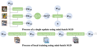
Figure 2: Local Training Configurations in Practical FL systems (take $E=1$ as an example).

4.1.1 Evaluate GIA against Multiple Updates

We consider a scenario where a client possesses $N$ data samples and configures $B=N$. Performing $U$ updates on $\mathbf{W}_{0}$, the client uploads $\mathbf{W}_{U}$ to the server. We start by conducting a theoretical analysis of the GIA concerning multiple local updates within the context of a binary classification problem. Subsequently, we provide empirical evaluations on practical classification tasks.

Theoretical Analysis. Consider a binary classification task ($y\in\{-1,1\}$) and a fully connected model with a single layer (ignoring the bias):

$$f\left(\mathbf{x}\right)=\mathbf{W}\mathbf{x},$$ (3)

where $\mathbf{W}$ represents the weight matrix and x denotes the input vector, $\mathbf{W},\mathbf{x}^{T}\in\mathbb{R}^{1\times n}$. The loss function $\ell$ can be expressed as:

$$\ell =\log\left(1+e^{-\mu}\right),\; \mu =y\mathbf{W}\mathbf{x}.$$ (4)

The gradient can be expressed as:

$$\frac{\partial\ell}{\partial\mathbf{W}}=y\frac{\partial\ell}{\partial\mu}\mathbf{x}^{T}.$$ (5)

The dependence between the gradient $\frac{\partial\ell}{\partial\mathbf{W}}$ and $\mu$ can be deduced as follows:

$$\frac{\partial\ell}{\partial\mathbf{W}}\cdot\mathbf{W}=y\frac{\partial\ell}{\partial\mu}\mathbf{x}^{T}\cdot\mathbf{W}=\frac{\partial\ell}{\partial\mu}\mu=\frac{-\mu}{1+e^{\mu}}.$$ (6)

Fig. 3 illustrates the dependence between gradient $\frac{\partial\ell}{\partial\mathbf{W}}$, $\mu$, and input $\mathbf{x}$. This implies that $\mu$ can be determined by the gradient $\frac{\partial\ell}{\partial\mathbf{W}}$ and weight $\mathbf{W}$ by Eq. (6), then $\mathbf{x}$ can be determined as follows:

$$x=y\mu\mathbf{W}^{T}.$$ (7)

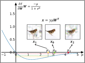
Figure 3: Dependence between Gradient $\frac{\partial\ell}{\partial\mathbf{W}}$, $\mu$ and Input $\mathbf{x}$. The ground-truth gradient corresponds to $\mu_{0}$, $\mathbf{x}_{0}$. When the gradients are obfuscated, they correspond to the inaccurate $\mu_{1}$, $\mu_{2}$, and $\mathbf{x}_{1}$, $\mathbf{x}_{2}$.

(1) If $U=1$:

The adversary can calculate the gradient $\frac{\partial\ell}{\partial\mathbf{W}_{0}}$ by $\frac{\mathbf{W}_{1}-\mathbf{W}_{0}}{\eta}$. Then, $\mu$ and $\mathbf{x}$ can be determined based on Eq. (6) and (7), respectively, as illustrated in Fig. 3 with $\mu_{0}$ and $\mathbf{x}_{0}$. This indicates that when the local training of clients involves only one update ($U=1$), a definite correspondence exists between the gradient and the input, enabling the adversary to deduce $x$ using an optimizer (e.g., Adam[45]) with gradient similarity as the loss function.

(2) If $U>1$:

In this case, the adversary can obtain $\mathbf{W}_{U}$ and $\mathbf{W}_{1}$, but does not know $U$. As shown in Eq. (8), the update after $U$ steps of mini-batch SGD is equal to:

$$\frac{\mathbf{W}_{U}-\mathbf{W}_{0}}{\eta}=\frac{\partial\ell}{\partial\mathbf{W}_{0}}+\frac{\partial\ell}{\partial\mathbf{W}_{1}}+\dots+\frac{\partial\ell}{\partial\mathbf{W}_{U-1}}$$ (8)

$$=\frac{\partial\ell}{\partial\mathbf{W}_{0}}+\sum_{u=1}^{U-1}\frac{\partial\ell}{\partial\mathbf{W}_{u}}\neq\frac{\partial\ell}{\partial\mathbf{W}_{0}}=\frac{\partial\ell}{\partial\mu_{0}}\mathbf{x}_{0}y.$$

However, the gradient $\frac{\mathbf{W}_{U}-\mathbf{W}_{0}}{\eta}$ includes $U-1$ redundant terms compared to the ground-truth gradient $\frac{\partial\ell}{\partial\mathbf{W}_{0}}$, thus leading to obfuscated $\mu$ and $\mathbf{x}$. Fig. 3 gives two examples where the gradients are incorrect due to the accumulated terms, which results in the solved $\mu_{1}$ and $\mu_{2}$ drifting from $\mu_{0}$. Thus, the reconstructed $\mathbf{x}_{1}$ and $\mathbf{x}_{2}$ also differ from $\mathbf{x}_{0}$. Hence, multiple local updates obfuscate the GIA.

Empirical Analysis. To empirically validate our theoretical conclusion, we evaluate the performance of the two SOTA GIAs (GIA-O with $p_{TV}$ and GIA-L with pretrained DcGAN[43]) as the number of local updates ($U$) increases on the datasets CIFAR10 ($N=B=4$) and CIFAR100 ($N=B=8$). We use the metric Learned Perceptual Image Patch Similarity (LPIPS)[49] to measure GIA’s performance, where a smaller value represents higher reconstruction quality. The detailed setup is described in Appendix. Tab. I demonstrates that when $U$ is 1 or 2, the adversary can still reconstruct the data. However, as $U$ increases, the LPIPS value exceeds $0.1$ (bold text in Tab. I), indicating that the reconstructed images are completely unrecognizable. Furthermore, the reconstruction quality deteriorates as $U$ increases, which indicates that the redundant terms in Eq. (8) gradually accumulate, and inaccuracy in the adversary’s update approximation grows.

TABLE I: GIA against Local Updates (LPIPS$\downarrow$).

Dataset	GIA	Number of Update ($U$)
		1	2	4	6	8
CIFAR10	GIA-O	0.0374	0.0933	0.1508	0.1917	0.2089
	GIA-L	0.0608	0.104	0.1332	0.1891	0.1917
CIFAR100	GIA-O	0.0061	0.0455	0.1248	0.163	0.2305
	GIA-L	0.0382	0.0578	0.1222	0.1712	0.1886

4.1.2 Evaluate GIA against Mini-Batch SGD

Here, we discuss a more practical scenario where the client has $N$ data samples and shares the $\textbf{W}_{U}$ after several local mini-batch SGD updates ($B<N,U=N/B$). It is crucial for the adversary to ascertain the value of $B$. Case 1: In the literature, it is assumed that the adversary knows $B$, enabling them to simulate the client’s mini-batch update using $N$ random initializations to more closely match $\frac{\mathbf{W}_{U}-\mathbf{W}_{0}}{\eta}$. Case 2: However, in practice, the client is not obligated to provide local training details to the server, thus the adversary can only approximate the update by conducting SGD ($B=N,U=1$) with $N$ samples. We evaluate GIAs in both cases, where the adversary has known or unknown $B$, as shown in Tab. II. We adjust the number of mini-batches by varying the value of $N/B$ on datasets CIFAR10 ($B=4$) and CIFAR100 ($B=8$).

The results show that under the same setting, successful reconstruction occurs if the adversary knows $B$ and executes the attack by simulating the local update process of the client (as described in Case 1). If B is unknown, reconstruction is still feasible with a limited number of mini-batches (e.g., $N/B=$ $1$ or $2$). However, as the number increases, reconstruction fails (indicated by the bold LPIPS value exceeding $0.1$), because solely relying on a single step of SGD to approximate the entire local training is insufficient (as described in Case 2).

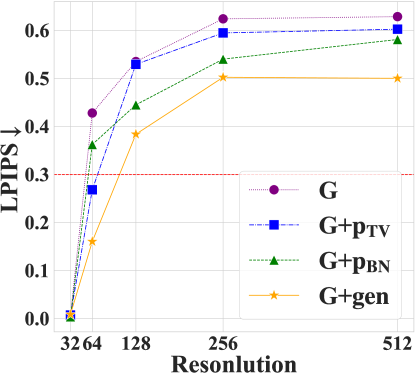
(a) GIA on Resolutions

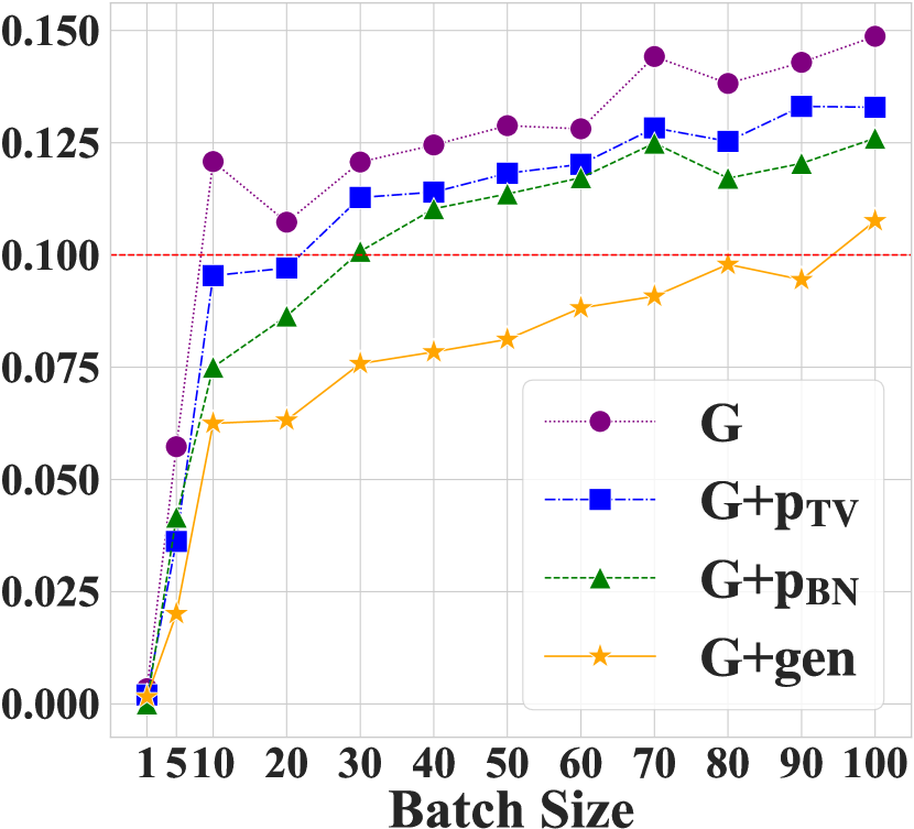
(b) GIA on Batch Sizes

Figure 4: GIA on Series of Data Dimensions.

TABLE II: GIA against Mini-Batch SGD (LPIPS$\downarrow$).

Dataset	GIA	$B$	Number of Mini-batch ($N/B$)
			1	2	3	4	5
CIFAR10	GIA-O	known	0.066	0.096	0.0696	0.0943	0.0931
		unknown	0.066	0.0961	0.1034	0.1142	0.1158
	GIA-L	known	0.0678	0.0534	0.0791	0.0647	0.0715
		unknown	0.0678	0.086	0.1089	0.105	0.1127
CIFAR100	GIA-O	known	0.0079	0.0534	0.0523	0.0395	0.0692
		unknown	0.0079	0.0431	0.058	0.1022	0.1145
	GIA-L	known	0.0325	0.0742	0.0409	0.051	0.0692
		unknown	0.0325	0.0774	0.0821	0.1016	0.1091

(Insight 4.1) The training configurations significantly impact GIA’s effectiveness. Specifically, as the number of local mini-batch SGD updates increases, the reconstruction of the training data becomes increasingly challenging.

4.2 Training Data

The primary goal of the GIA revolves around reconstructing training data. To investigate its impact, we evaluate the performance of GIAs on two basic data properties, dimension and content. First, we empirically evaluate the impact of training data on GIAs across various resolutions and batch sizes in practical FL systems. Subsequently, we look into the influence of image content on GIAs—an aspect largely overlooked in existing literature [20, 2, 3, 4, 6].

4.2.1 Reconstructing Data with Wide Dimensions

In CV tasks, data dimension is related to resolution and batch size. Here, we demonstrate how GIAs perform across diverse dimensional settings (batch size 1$\sim$100, image resolution 32$\times$32$\sim$512$\times$512). We evaluate the baseline G (GIA-O with only gradient-matching loss) and three SOTA GIAs: G+$p_{TV}$ (GIA-O with prior total variation[2]), G+$p_{BN}$ (GIA-O with prior BN statistics[3]), and G+gen (GIA-L with generative knowledge[4, 5]).

Experimental Setup: We evaluate GIAs under FedSGD[92] using ResNet-18 on CIFAR10, CIFAR100, and ImageNet-1K[42]. The performance of GIA is measured by LPIPS. Detailed setup is provided in Appendix.

Fig. 4 illustrates the statistical results, some snapshots of which are shown in Fig. 5. Our findings indicate that (1) GIA performs well in reconstructing low-dimensional data (resolution $<64\times 64$ and batch size $<30$), but has difficulty in reconstructing high-dimensional data. Fig. 4(a) shows that the adversary could reconstruct images with resolutions less than $64\times 64$ pixels, but all four methods fail to reconstruct an image with an acceptable quality (i.e., LPIPS greater than 0.3) when the pixel value is larger than $128\times 128$. As for Fig. 4(b), bounded by LPIPS = 0.1, we find that GIA-Os are still able to reconstruct with batch sizes smaller than 30, but as the batch size increases, only GIA-L can reconstruct successfully. (2) GIA-L presents a better performance in reconstructing high-dimensional data compared to GIA-O. As Fig. 4 shows, GIA-L can reconstruct data with batch size over $90$ (Fig. 4(b)). As depicted in Fig. 5, although GIA-L is unable to reconstruct high-resolution images with high overall similarity (low LPIPS), it can still capture the semantic information within them. In contrast, GIA-Os completely fail in this aspect. GIA-L benefits from two aspects: First, GIA-L has a smaller search space, which allows the optimizer to better find the optimal. Second, generative knowledge guarantees the fidelity.

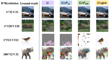
Figure 5: Snapshots of Fig. 4.

(Insight 4.2.1) For low-dimensional data, GIAs can conduct effective reconstruction. However, for high-dimensional data, GIA-L can only achieve a semantic-level reconstruction coarsely, while GIA-O struggles to reconstruct any recognizable information.

4.2.2 Reconstructing Data with Various Contents

In practical scenarios, a client may hold training data with various contents, potentially affecting GIA’s performance. Sincerely, the effectiveness of GIAs is truly represented by their ability to reconstruct semantic details containing important private information. Fig. 6 demonstrates the reconstruction of face images. Although the reconstructed results may achieve relatively high similarity, they represent trivial privacy leakage only due to differences in facial details. Meanwhile, GIA-L utilizes public data to train generators and aims to reconstruct clients’ private data. The gap between the two data distributions affects the performance of GIA-L. Fig. 6 shows that reconstructing out-of-distribution (OOD) images is much harder than reconstructing identical-distribution (ID) ones. In this subsection, we evaluate GIAs in reconstructing data containing abundant semantic details and in out-of-distribution (OOD).

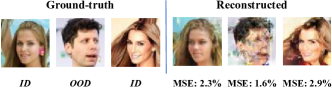
Figure 6: Semantic Details and Distribution Impact Privacy Risk.

i@. Semantic details in data diminish the effectiveness of GIAs. To reveal the impact of semantic details on GIAs, we choose two types of attacks: GIA-O with priors including both $p_{TV}$ and $p_{BN}$, and GIA-L with BigGAN’s generator[44] pre-trained on ImageNet-1K[42]. The experiments are conducted on ImageNet-1K dataset, and setup details are provided in the Appendix. As shown in Fig. 7, the reconstructed images reveal very little private information because all the crucial details are lost. Specifically, Fig. 7 (a)-(c) show the results of reconstructing clock images. We observe that GIA-L can reconstruct certain features, such as colors and backgrounds. However, it fails to reconstruct crucial semantic details, such as the correct time (e.g., incorrect hand pointing in Fig. 7 (b),(c)). The neglect of semantic details is further exemplified in Fig. 7 (d)-(f), where only the backgrounds are successfully reconstructed, while other crucial contents (e.g., numbers, text) are completely lost. In addition, we find that images with semantic details tend to mislead GIAs. As shown in Fig. 7 (g)-(i), the ruler with dense scales and the scoreboard with complex content lead to misinterpretation of GIA-L. Moreover, the panel results in completely failed reconstructions. The reasons for GIA’s negligence of semantic details stem from two aspects: (1) the gradient reflects more the model’s capture of category features than semantic details; (2) the pre-trained generator only learns class-wise features rather than identical details.

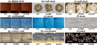
Figure 7: Failure to Reconstruct Semantic Details, Limited Privacy Leakage. (Left: Ground-Truth, Middle: Results of GIA-O, Right: Results of GIA-L, LPIPS$\downarrow$).

(Insight 4.2.2) (1) GIAs cannot guarantee the accurate reconstruction of intricate semantic details, which potentially contain crucial private information.

ii@. OOD data impedes the generalization capability of GIA-L. OOD generalization represents an evolving research area within machine learning, where the distributions of the test data diverge from those of the training data[53, 54]. In FL scenarios, adversaries undertake the GIA-L by pre-training a generator on collected data, whose distribution is practically different from the client’s data distribution, thus introducing a potential OOD challenge. However, the OOD problem of GIA-L has not been well discussed. Therefore, we propose a novel OOD-Test Set, and then conduct an empirical evaluation to examine the generalization capability of the GIA-L.

Our OOD-Test Set consists of four distinct OOD types, designed to evaluate GIA’s reconstruction and generalization performance in diverse contents.

$\bullet$ Places tests the performance of GIA-L in images involving complex background information. It is a subset of Places365[55] curated by Huang et al.[56] with 9822 typical environments from 50 categories that are not present in ImageNet-1K[42], which has been widely used as OOD test sets in recent works[56, 57, 58]. Here, we showcase two representative samples from categories hayfield and lagoon&ocean in Fig. 8.

$\bullet$ Textures tests the performance of GIA-L in reconstructing complicated patterns. The dataset includes 5,640 images across 47 texture categories[59]. Here, we showcase two representative samples from categories bubbly and honeycombed in Fig. 8.

$\bullet$ Objects tests the performance of GIA-L in reconstructing objects with different characteristics but similar labels. It contains 2000 images from ImageNet-21K, excluding its subset ImageNet-1K[60]. Here, we showcase two representative samples from categories echinoderm and pickle in Fig. 8.

$\bullet$ Styles tests the cross-style generalization of GIA-L. It contains 9991 images from 7 categories and 4 styles (photo, art painting, cartoon, and sketch)[61]. Here, we showcase two representative samples from styles art painting and cartoon in Fig. 8.

Fig. 8 demonstrates the reconstruction performance of GIA-L on ID and OOD data, respectively. The results indicate that GIA-L performs badly on OOD data due to its limited generative capability. For each pair of samples labeled similarly, the LPIPS values for reconstructing ID data are significantly lower than those of reconstructing OOD images. In the case of Textures and Styles, each image pair shares identical labels but exhibits significant differences in feature space. For instance, natural bubbles display a range of characteristics, such as “discrete and transparent” or “dense and blue”, as demonstrated for bubble and bubbly in Fig. 8, respectively. Another example involves varying styles of guitars. GIA-L can only reconstruct broadly recognizable features like strings and sound holes but fails to accurately depict the appearance of a guitar in art or cartoon style.

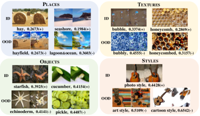
Figure 8: Gallery of OOD-Test Set and Reconstruction Performance of GIA-L. (Left: Ground-Truth, Right: Reconstructed Image, LPIPS$\downarrow$. Each column is a pair of samples with similar labels, Up: Sample from ImageNet-1K[42](ID) dataset, Bottom: Sample from the OOD dataset).

(Insight 4.2.2) (2) GIA-L demonstrates limited generalization capabilities and struggles to reconstruct OOD data effectively.

5 Evaluation on Model

The model determines the mapping from training data to the gradient. During the FL training phase, the adversary acquires a specific model and its corresponding gradient at a particular stage (round) for GIAs. In this section, we investigate the impact of the model on gradient inversion from the perspectives of stage and architecture. To illustrate and quantify the model’s vulnerability to GIAs, we introduce a novel Input-Gradient Smoothness Analysis (IGSA) method. Through IGSA, we empirically assess the resistance of nine models against GIAs at different stages (rounds) during the FedAvg training phase. Subsequently, we explore the performance of GIAs on prevalent model structures and micro designs, thereby revealing the sensitivity of GIAs to model architecture.

5.1 Training Stage

5.1.1 Input-Gradient Smoothness Analysis (IGSA)

The model $W$ defines the objective function for the GIA, which is composed of the “input-gradient” function $\Phi\left(\cdot\right)$ (comprising forward and backward propagation) and the subsequent gradient matching $Dist\left(\cdot,\cdot\right)$. Hence, to investigate the impact of the model on gradient inversion, we initiate our exploration by examining the properties of its objective function, with a specific focus on $\Phi\left(\cdot\right)$.

The smoothness of the objective function determines the difficulty in locating the global optimum[108]. Fig. 9 examples of the landscape of $\Phi\left(\cdot\right)$. For a given function, its landscape can be smooth or oscillatory. A smooth function, characterized by gently varying gradients, facilitates the identification of the global optimum. Correspondingly, the reconstructed image becomes clearer as the loss decreases, as demonstrated in Fig. 9(a). In contrast, an oscillatory function, marked by dramatically varying gradients, leads to local optima and disrupts the optimization process[12]. Fig. 9(b) illustrates how the oscillatory landscape complicates the task of locating the best reconstruction.

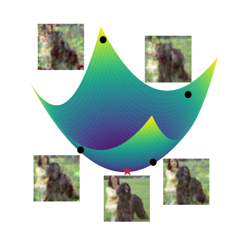
(a) Smooth Landscape

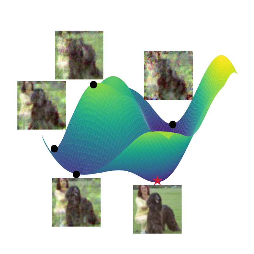
(b) Oscillatory Landscape

Figure 9: Examples of Objective Function’s Landscape.

Therefore, we propose a novel method termed IGSA to characterize the model’s resilience to GIAs. First, we employ the Jacobi matrix to compute the first-order differentiation of the “input-gradient” function $\Phi\left(\cdot\right)$, which reflects how drastically the gradient changes in response to input perturbations:

$$\mathbf{J}(\mathbf{X})=\frac{\partial\Phi(\mathbf{X})}{\partial\mathbf{X}}.$$ (9)

Afterward, we utilize $K$ samples located within a radius $r$ of $\mathbf{X}$ to estimate the IGSA values. Moreover, considering that the gradients span across $L$ layers, we construct a vector $\omega=\text{SoftMax}\left(\left[L,L-1,\ldots,1,0\right]\right)$. This vector assigns a greater weight to the shallow layers when averaging $l_{2}$-norms.

$$IGSA^{\mathbf{X}} =\frac{1}{\mathbf{\mathbb{E}}_{\Delta x}\left[\left\|\Phi(\mathbf{X})-\Phi(\mathbf{X}+\Delta\mathbf{X})\cdot\omega\right\|_{2}\right]}$$ (10)

$$=\frac{K}{\sum_{k=1}^{K}\left\|\mathbf{J}\left(\mathbf{X_{k}}\right)\cdot\omega\right\|_{2}}.$$

A higher IGSA value indicates that $\Phi\left(\cdot\right)$ possesses a greater degree of smoothness. which makes it easier for the adversary to locate and reconstruct training data.

5.1.2 Evaluating Model’s Vulnerability to GIA in Different Stages

In this part, we analyze and explain the model’s vulnerability to GIAs at different stages of the training process in FL. We choose $9$ models from four families that are widely used in vision tasks, i.e., VggNets-(11, 16, 19)[50], ResNets-(18, 50, 152), DenseNet121[67], and InceptionNets (GoogleNet[68] and Inception-v3[69]).

Experimental setup: We evaluate nine models using the CIFAR10 dataset in the FedAvg setting. Each model undergoes $100$ training rounds. During each round, we launch GIA on the current model, whose performance is measured by PSNR (Peak Signal-to-Noise Ratio) while simultaneously assessing the model accuracy and IGSA value. To enhance clarity in presentation, we average the results every five rounds in Fig. 10. Further details are provided in Appendix.

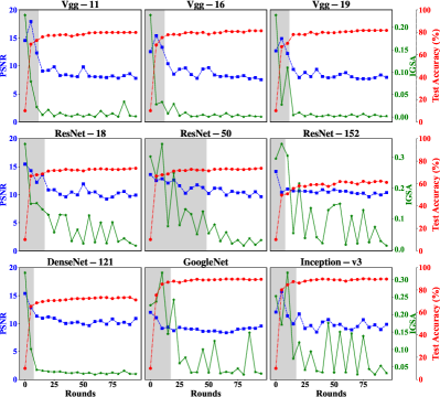
Figure 10: Model’s Resistance to GIA during FL Training. Model’s test accuracy: Test Accuracy$\uparrow$, reconstruction quality: PSNR$\uparrow$, resistance to GIA: IGSA$\downarrow$. Gray areas represent the rounds where GIA is valid, and the other areas represent the rounds where GIA is not valid. Every point is an average of five rounds.

Fig. 10 illustrates the resilience of the nine models against the GIA during training. We can intuitively observe that gradient inversion only works in the early stages of FL training. For instance, in the case of the Vgg-11 model, initially, the PSNR value is high, but as the training process continues, it consistently stays below $10$ after approximately $15$ rounds, indicating a diminished leakage of private information in the reconstructed images.

Moreover, by combining the test accuracy curves, we note that the rounds where the GIA poses a threat often align with those wherein the model is under-fitting. Once the accuracy stabilizes (indicating well-fitting), the model exhibits enhanced resistance to the GIA. Additionally, the IGSA curves exhibit distinct phases, where the reconstruction quality is acceptable when IGSA values remain high. Conversely, reconstruction tends to fail when IGSA curves drop and fluctuate at lower levels.

(Insight 5.1) During FL training, GIA primarily compromises the privacy of training data in the early stages when the model is under-fitting. Once the training accuracy stabilizes, it is difficult for the adversary to invert any private information from the gradient.

5.2 Model Architecture

The model architecture determines the flow of information and the extraction of features, further influencing the path of backpropagation and gradient computation, thereby potentially affecting GIAs. In this subsection, we study the impact of model architecture on the GIA from two perspectives: structures and micro designs.

5.2.1 Model Structure: A Double-edged Sword

Model structure refers to the way layers are connected to each other. Early models such as Vgg[50] were sequentially connected. Later, in order to mitigate gradient vanishing[48] and enhance feature extraction capabilities, skip[48] and parallel[68] structures began to appear and gradually became the backbone of model designs. In this subsection, we explore the effect of model structures on the GIA with two widely used cases in practice: skip connection[48] (used in models like ResNet and DenseNet families) and net-in-net[68] (used in models like GoogleNet and other InceptionNet families).

i@. Skip connection is a widely used structure in deep neural networks that helps address gradient vanishing during training[48]. It enables the flow of features from one layer to another by creating direct connections between non-adjacent layers. Generally, there are two common types of skip connections, derived from ResNet and DenseNet, as shown in Fig. 11. In ResNet, skip connections take the form of identity mappings, where the input to a layer is added directly to the output of the subsequent layer. In contrast, DenseNet takes a more aggressive approach by densely concatenating all previous layers within a block, enhancing feature reuse [67].

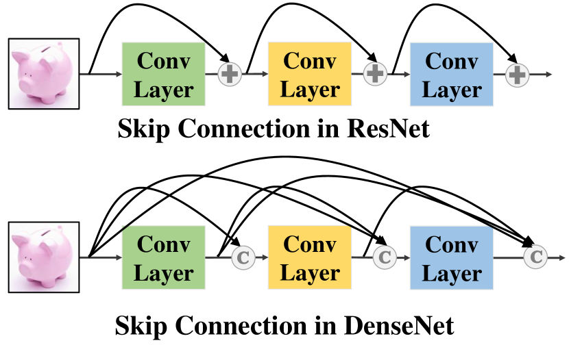
(a) Skip Connection

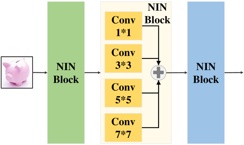
(b) Net-in-Net

Figure 11: Two Widely Used Model Structures.

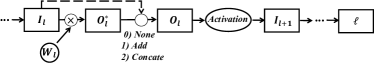
Figure 12: A Layer in Deep Neural Network with Three Types of Connections. 0) no skip connection, no additional operation; 1) ResNet-like skip connection, feature adding; 2) DenseNet-like skip connection, feature concatenation.

To illustrate how skip connections affect the GIA, we start with a derivation on how they affect backpropagation. Fig. 12 illustrates a particular layer ($\mathbf{I}_{l}$ and $\mathbf{O}_{l}$ represent the input and output of layer $l$, respectively), which may have three types of connections: normal (sequential), ResNet-like, and DenseNet-like. Then, the process of backpropagation can be presented in three cases:

For normal case, $\mathbf{O}^{*}_{l}=\mathbf{O}_{l}$:

$$\frac{\partial\ell}{\partial\mathbf{I}_{l}}=\frac{\partial\ell}{\partial\mathbf{I}_{l+1}}\frac{\partial\mathbf{I}_{l+1}}{\partial\mathbf{I}_{l}}=\frac{\partial\ell}{\partial\mathbf{I}_{l+1}}\frac{\partial\mathbf{I}_{l+1}}{\partial\mathbf{O}_{l}}\mathbf{W}_{l}.$$ (11)

For ResNet and DenseNet, the gradient in the deeper layers is passed to the front layers by adding or concatenation ( $\boldsymbol{\oplus}$ represents both operations in Eq. (12)):

$$\begin{split}\frac{\partial\ell}{\partial\mathbf{I}_{l}}&=\frac{\partial\ell}{\partial\mathbf{I}_{l+1}}\frac{\partial\mathbf{I}_{l+1}}{\partial\mathbf{I}_{l}}=\frac{\partial\ell}{\partial\mathbf{I}_{l+1}}\frac{\partial\mathbf{I}_{l+1}}{\partial\mathbf{O}_{l}}\frac{\partial\mathbf{O}_{l}}{\partial\mathbf{I}_{l}}\\ &=\frac{\partial\ell}{\partial\mathbf{I}_{l+1}}\frac{\partial\mathbf{I}_{l+1}}{\partial\mathbf{O}_{l}}\frac{\partial(\mathbf{O}_{l}^{*}\oplus\mathbf{I}_{l})}{\partial\mathbf{I}_{l}}=\frac{\partial\ell}{\partial\mathbf{I}_{l+1}}\frac{\partial\mathbf{I}_{l+1}}{\partial\mathbf{O}_{l}}(\mathbf{W}_{l}\underline{\oplus\textbf{1}}).\end{split}$$ (12)

Compared with Eq. (11), there is one more residual term in the gradient of Eq. (12). For models with skip connections, residual terms multiply cumulatively with backpropagation so that the gradient could contain more combinations, which prevents the gradient from vanishing and likewise benefits GIAs by allowing them to utilize more information.

We then verify the effect of skip connections on GIA based on ResNets and DenseNets, respectively. First, we evaluate how cutting skip connections at different positions affects the GIA on ResNet-18 and ResNet-34, as shown in Fig. 13. We find that (1) the presence of skip connections enhances the performance of the GIA. Fig. 13 demonstrates that the original models (i.e., N) are much more vulnerable to the GIA than others with connection cuts. Moreover, cutting the skip connection at any position significantly worsens the effectiveness of the GIA, even resulting in failed reconstruction (LPIPS $>0.1$). In addition, we find that (2) skip connections close to shallow or deep layers have a greater impact on the GIA. Fig. 13(b) shows that cutting shallow connections ($\#0,1,2$) and deep connections ($\#12,14,15$) drastically worsen the performance of the GIA. For shallower connections, recent works [71, 72, 73] regarding information flow in deep neural networks state that shallow layers are more sensitive to the input, and so are their gradients, which benefits GIAs. For deeper connections, inspired by Eq. (12), since the gradients are computed from deep to shallow, the absence of deeper residual terms has a more significant effect on the whole gradient and so on the GIA, like dominoes.

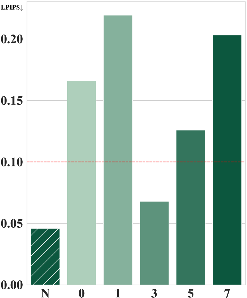
(a) ResNet-18

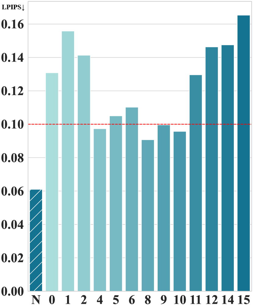
(b) ResNet-34

Figure 13: Position of Skip Connections Affects GIA. N (No Cut) represents the original model with full skip connections, and thereafter Id represents the model cutting the Id connection, with darker colors representing deeper positions.

Besides, we explore the impact of the number of skip connections on the GIA with DenseNets, considering their dense nature. We select DenseNet-43 and DenseNet-53[74] as baselines and obtain two variants for each by employing different cutting strategies[74]. As shown in Fig. 14, reducing the number of skip connections greatly affects the performance of GIAs. Images that can be easily inverted in baselines are largely unrecognizable in variants-1. Moreover, GIAs are completely unable to invert any information from variants-2. Reducing the number of skip connections in a neural network model decreases both the backpropagation paths and the residual terms. This leads to the gradients becoming less informative, which in turn limits the effectiveness of GIAs.

(Insight 5.2.1) (1) Skip connections alleviate gradient vanishing (Pros), while increasing the path of backpropagation and introducing residual terms, which enables the adversary to obtain more information from gradients (Cons).

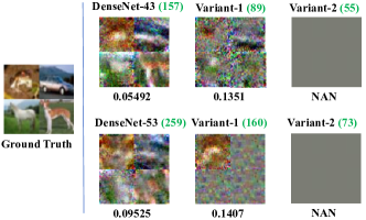
Figure 14: Number of Skip Connections Affects GIA. Green number represents the number of skip connections contained. LPIPS$\downarrow$.

ii@. Net-in-net (NIN), as proposed in [68], is a module that integrates multi-scale convolutional kernels within a single block, as illustrated in Fig. 11(b). Essentially, NIN works like a widening layer, where the multi-scale convolutional kernel can capture richer features from the input. However, it is evident that wider layers and multi-scale kernels also yield more informative gradients through backpropagation, consequently enhancing the effectiveness of GIAs.

To further demonstrate NIN’s enhancement in GIA’s performance, we conduct ablation studies on GoogleNet and InceptionNet-V3, as detailed in Tab. III. Specifically, we compare the reconstruction results obtained using the complete gradients versus solely the gradients from a single NIN block. These findings validate that the gradients from NIN blocks are crucial to the model’s vulnerability to the GIA. For example, as shown in Tab. III, although we only use the gradient of the $\#1$ NIN block in GoogleNet, which constitutes merely $2.27\%$ of the total parameters, we achieve a result nearly equivalent to that obtained with the full gradient (a comparison of $0.0654$ to $0.0614$). This observation indicates that the gradient from a single NIN block poses a privacy risk comparable to the entire gradients despite its relatively minor proportion, suggesting the presence of a NIN block is essential for GIAs.

TABLE III: The Performance of GIA Using Full or a Single NIN Block’s gradient.

Model	Metric	Used Gradient
		Full	#1 NIN Block’s	#2 NIN Block’s	#3 NIN Block’s	#4 NIN Block’s
GoogleNet	Params(Ratio)	54,909,86(100.00%)	149,376(2.72%)	640,848(11.68%)	60,928(6.58%)	508,032(9.25%)
	LPIPS$\downarrow$	0.0614±0.003	0.0654+0.004	0.0667±0.001	0.0710±0.005	0.0620±0.006
Inception V3	Params(Ratio)	21,638,954(100.00%)	246,688(1.14%)	336,640(1.56%)	381,440(1.76%)	1,138,528(5.26%)
	LPIPS$\downarrow$	0.0332±0.004	0.0472±0.001	0.0435±0.002	0.0433±0.003	0.0360±0.005

(Insight 5.2.1) (2) NIN utilizes multi-scale kernels for stronger feature extraction capability (Pros), while requiring different updates to multiple kernels during backpropagation, which provides informative gradient to benefit GIAs (Cons).

5.2.2 Micro Design: Tiny Clue Reveals the General Trend

Micro designs are subtle techniques ubiquitous in nearly all modern models. To investigate their impact on the GIA, we evaluate six prevalent micro designs: bias, activation function (ReLU), dropout, max pooling, convolutional kernels (size), and padding. In particular, we make a series of modifications to a configurable model, ConvNet[2], which only includes components related to micro designs. In this way, we can control variables and check the resistance of the specific micro design to the GIA. The standard ConvNet incorporates bias, employs ReLU functions, and includes two max pooling layers and one dropout layer. Additionally, all convolutional layers are equipped with $3\times 3$ kernels and padding ($1$). Details are provided in Appendix.

TABLE IV: The Performance of GIA with Various Modifications to ConvNet. (+): Modifications improve the quality of reconstruction, (–): Modifications reduce the quality of reconstruction. (R)emove, (I)ncrease, (D)ecrease.

Modifications	None	R ReLU (+)	R DropOut (+)	R MaxPool2d (+)	I kernel to $4\times 4$ (+)
LPIPS$\downarrow$	0.0080±0.0005	0.0008±0.0003	0.0048±0.0007	0.0003±0.0001	0.0022±0.0007
Modifications	R bias (–)	D kernel to $2\times 2$ (–)	D kernel to $1\times 1$ (–)	I padding to 2 (–)	I padding to 3 (–)
LPIPS$\downarrow$	0.0280±0.0004	0.0251±0.0006	0.2139±0.0008	0.0091±0.0002	0.0203±0.0005

Our findings indicate that micro designs significantly impact the model’s resistance to the GIA. As shown in Tab. IV, removing ReLU, dropout, max pooling layers, or increasing the kernel size substantially exacerbates the model’s vulnerability to GIAs. In contrast, removing bias, decreasing the kernel size or expanding padding enhances the model’s resilience to GIAs.

Essentially, micro design affects the amount of information available in the feature map. Specifically, reducing the information content of the feature map related to the input would render GIAs less effective. (1) Feature map sparsification. The activation function induces a nonlinear transformation of elements in the feature map, dropout zeroes out certain elements, and padding effectively “dilutes” the original feature map. (2) Feature map aggregation. The max pooling layer selects representative elements, and a smaller kernel size focuses on more localized features. These designs reduce the correlation between the input and the feature maps, and thus it is difficult to invert the accurate input data through the gradient. However, enhancing the information content of the feature map benefits GIAs. The increase of kernel size would promote the model in extracting features on a broader scale, thereby augmenting the information within the feature map, while bias provides extra parameters, which indirectly benefits the GIAs. (Insight 5.2.2) Micro designs influence the amount of information shared between the model’s feature maps and the input, consequently affecting the gradient and substantially impacting the performance of GIAs.

6 Evaluation on Post-Processing

In practical FL systems, clients often apply post-processing techniques to gradients before sharing them with the server. These methods obfuscate the shared gradients to offer potential defense for clients against GIAs. In this section, we study the effectiveness of four commonly utilized post-processing techniques in defending against GIAs under a practical FL setting. Moreover, we evaluate their capacity to address the critical trade-off between the model utility and defensive performance.

Experimental setup: We consider a practical FL system that involves $100$ clients collaboratively training ResNet-18 and ResNet-34 models using the CIFAR10 and CIFAR100 datasets. The server launches two SOTA GIAs: GIA-O and GIA-L. To defend against these attacks, the client employs four post-processing techniques on the gradient: quantization (Q)[77], sparsification (S)[80], clipping (C)[81], and perturbation (P)[82]. Details can be found in Appendix.

We conduct experiments to assess the efficacy of four post-processing techniques against GIAs and their impact on accuracy under different parameter settings (shown in Appendix). We choose the optimal performance for each post-processing technique, representing the best privacy-utility trade-off, and present these results in Fig. 15. We show that: most post-processing techniques can effectively defend against the strongest GIAs without significantly compromising accuracy. This is illustrated by their points distributed above the blue line and to the right of the red line. Among these techniques, quantization demonstrates the most favorable trade-off. In the experiment involving ResNet-18 and CIFAR100 (Figure 15), utilizing $2$-bit quantization on shared gradients enables clients to defend against GIAs with an accuracy drop of no more than 5%. However, clipping fails to guarantee the trade-off. As shown in Figure LABEL:pic:P18_10, even with a large clip value that significantly impacts accuracy (dropping from 80% to about 40%), it has almost no effect on GIAs.

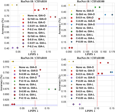
Figure 15: Best Results That Maintain Privacy-Utility Tradeoff in FL Systems Utilizing Various Post-Processings. Red Line is a split line of privacy leakage. Blue Line is a split line of model’s acceptable utility.

(Insight 6) In practical FL systems, even trivial post-processings applied to gradients can easily defend against the most powerful GIAs while maintaining model accuracy.

7 Conclusion

In this work, we conducted a comprehensive study on GIAs in practical FL. We thoroughly reviewed the development of the GIA so far, highlighting the milestones and breakthroughs. Moreover, we established a systematization of GIAs to uncover their inherent threats. We indicated that the notable effectiveness demonstrated by current GIAs relies on ideal settings with auxiliary assumptions. To assess the actual threat of GIAs against practical FL systems, we identified the challenges GIAs face in practice from three crucial aspects: local training, model, and post-processing. By conducting theoretical and empirical evaluations of state-of-the-art GIAs in diverse settings, our findings indicate that the actual threat posed by GIAs to practical FL systems is limited, despite their perceived potency in the existing literature. We aim for our work to rectify previous misconceptions to some extent and stimulate more accurate and realistic investigations into GIAs in FL.

References

- [1] G. D. Greenwade, “The Comprehensive Tex Archive Network (CTAN),” TUGBoat, vol. 14, no. 3, pp. 342–351, 1993.
- [2] J. Geiping, H. Bauermeister, H. Dröge, and M. Moeller, “Inverting gradients-how easy is it to break privacy in federated learning?” Advances in Neural Information Processing Systems, vol. 33, pp. 16 937–16 947, 2020.
- [3] H. Yin, A. Mallya, A. Vahdat, J. M. Alvarez, J. Kautz, and P. Molchanov, “See through gradients: Image batch recovery via gradinversion,” in Proceedings of the IEEE/CVF Conference on Computer Vision and Pattern Recognition, 2021, pp. 16 337–16 346.
- [4] J. Jeon, K. Lee, S. Oh, J. Ok et al., “Gradient inversion with generative image prior,” Advances in neural information processing systems, vol. 34, pp. 29 898–29 908, 2021.
- [5] Z. Li, J. Zhang, L. Liu, and J. Liu, “Auditing privacy defenses in federated learning via generative gradient leakage,” in Proceedings of the IEEE/CVF Conference on Computer Vision and Pattern Recognition, 2022, pp. 10 132–10 142.
- [6] A. Hatamizadeh, H. Yin, H. R. Roth, W. Li, J. Kautz, D. Xu, and P. Molchanov, “Gradvit: Gradient inversion of vision transformers,” in Proceedings of the IEEE/CVF Conference on Computer Vision and Pattern Recognition, 2022, pp. 10 021–10 030.
- [7] S. Gupta, Y. Huang, Z. Zhong, T. Gao, K. Li, and D. Chen, “Recovering private text in federated learning of language models,” Advances in Neural Information Processing Systems, vol. 35, pp. 8130–8143, 2022.
- [8] J. Lu, X. S. Zhang, T. Zhao, X. He, and J. Cheng, “April: Finding the achilles’ heel on privacy for vision transformers,” in Proceedings of the IEEE/CVF Conference on Computer Vision and Pattern Recognition, 2022, pp. 10 051–10 060.
- [9] M. Balunovic, D. Dimitrov, N. Jovanović, and M. Vechev, “Lamp: Extracting text from gradients with language model priors,” Advances in Neural Information Processing Systems, vol. 35, pp. 7641–7654, 2022.
- [10] Y. Liu, B. Ren, Y. Song, W. Bi, N. Sebe, and W. Wang, “Breaking the chain of gradient leakage in vision transformers,” arXiv preprint arXiv:2205.12551, 2022.
- [11] M. Vero, M. Balunović, D. I. Dimitrov, and M. Vechev, “Data leakage in tabular federated learning,” arXiv preprint arXiv:2210.01785, 2022.
- [12] E. K. Chong and S. H. Żak, An introduction to optimization. John Wiley & Sons, 2013, vol. 75.
- [13] R. C. Geyer, T. Klein, and M. Nabi, “Differentially private federated learning: A client level perspective,” arXiv preprint arXiv:1712.07557, 2017.
- [14] Y. Lin, S. Han, H. Mao, Y. Wang, and W. J. Dally, “Deep gradient compression: Reducing the communication bandwidth for distributed training,” arXiv preprint arXiv:1712.01887, 2017.
- [15] B. McMahan, E. Moore, D. Ramage, S. Hampson, and B. A. y Arcas, “Communication-efficient learning of deep networks from decentralized data,” in Artificial intelligence and statistics. PMLR, 2017, pp. 1273–1282.
- [16] S. Banabilah, M. Aloqaily, E. Alsayed, N. Malik, and Y. Jararweh, “Federated learning review: Fundamentals, enabling technologies, and future applications,” Information processing & management, vol. 59, no. 6, p. 103061, 2022.
- [17] B. McMahan and A. Thakurta, “Federated learning with formal differential privacy guarantees,” Google AI Blog, 2022.
- [18] A. Hard, K. Rao, R. Mathews, S. Ramaswamy, F. Beaufays, S. Augenstein, H. Eichner, C. Kiddon, and D. Ramage, “Federated learning for mobile keyboard prediction,” arXiv preprint arXiv:1811.03604, 2018.
- [19] L. Zhu, Z. Liu, and S. Han, “Deep leakage from gradients,” Advances in neural information processing systems, vol. 32, 2019.
- [20] Z. Wang, M. Song, Z. Zhang, Y. Song, Q. Wang, and H. Qi, “Beyond inferring class representatives: User-level privacy leakage from federated learning,” in IEEE INFOCOM 2019-IEEE conference on computer communications. IEEE, 2019, pp. 2512–2520.
- [21] B. Li, P. Qi, B. Liu, S. Di, J. Liu, J. Pei, J. Yi, and B. Zhou, “Trustworthy ai: From principles to practices,” ACM Computing Surveys, vol. 55, no. 9, pp. 1–46, 2023.
- [22] F. Boenisch, A. Dziedzic, R. Schuster, A. S. Shamsabadi, I. Shumailov, and N. Papernot, “When the curious abandon honesty: Federated learning is not private,” in 2023 IEEE 8th European Symposium on Security and Privacy (EuroS&P). IEEE, 2023, pp. 175–199.
- [23] B. Zhao, K. R. Mopuri, and H. Bilen, “idlg: Improved deep leakage from gradients,” arXiv preprint arXiv:2001.02610, 2020.
- [24] D. C. Liu and J. Nocedal, “On the limited memory bfgs method for large scale optimization,” Mathematical programming, vol. 45, no. 1-3, pp. 503–528, 1989.
- [25] L. I. Rudin, S. Osher, and E. Fatemi, “Nonlinear total variation based noise removal algorithms,” Physica D: nonlinear phenomena, vol. 60, no. 1-4, pp. 259–268, 1992.
- [26] Y. Huang, S. Gupta, Z. Song, K. Li, and S. Arora, “Evaluating gradient inversion attacks and defenses in federated learning,” Advances in Neural Information Processing Systems, vol. 34, pp. 7232–7241, 2021.
- [27] J. Geng, Y. Mou, F. Li, Q. Li, O. Beyan, S. Decker, and C. Rong, “Towards general deep leakage in federated learning,” arXiv preprint arXiv:2110.09074, 2021.
- [28] D. I. Dimitrov, M. Balunovic, N. Konstantinov, and M. Vechev, “Data leakage in federated averaging,” Transactions on Machine Learning Research, 2022.
- [29] J. Xu, C. Hong, J. Huang, L. Y. Chen, and J. Decouchant, “Agic: Approximate gradient inversion attack on federated learning,” in 2022 41st International Symposium on Reliable Distributed Systems (SRDS). IEEE, 2022, pp. 12–22.
- [30] L. Fan, K. W. Ng, C. Ju, T. Zhang, C. Liu, C. S. Chan, and Q. Yang, “Rethinking privacy preserving deep learning: How to evaluate and thwart privacy attacks,” Federated Learning: Privacy and Incentive, pp. 32–50, 2020.
- [31] J. Zhu and M. Blaschko, “R-gap: Recursive gradient attack on privacy,” arXiv preprint arXiv:2010.07733, 2020.
- [32] L. Fowl, J. Geiping, W. Czaja, M. Goldblum, and T. Goldstein, “Robbing the fed: Directly obtaining private data in federated learning with modified models,” arXiv preprint arXiv:2110.13057, 2021.
- [33] H.-M. Chu, J. Geiping, L. H. Fowl, M. Goldblum, and T. Goldstein, “Panning for gold in federated learning: Targeted text extraction under arbitrarily large-scale aggregation,” in The Eleventh International Conference on Learning Representations, 2022.
- [34] L. Fowl, J. Geiping, S. Reich, Y. Wen, W. Czaja, M. Goldblum, and T. Goldstein, “Decepticons: Corrupted transformers breach privacy in federated learning for language models,” arXiv preprint arXiv:2201.12675, 2022.
- [35] D. Pasquini, D. Francati, and G. Ateniese, “Eluding secure aggregation in federated learning via model inconsistency,” in Proceedings of the 2022 ACM SIGSAC Conference on Computer and Communications Security, 2022, pp. 2429–2443.
- [36] Y. Wen, J. Geiping, L. Fowl, M. Goldblum, and T. Goldstein, “Fishing for user data in large-batch federated learning via gradient magnification,” arXiv preprint arXiv:2202.00580, 2022.
- [37] J. C. Zhao, A. R. Elkordy, A. Sharma, Y. H. Ezzeldin, S. Avestimehr, and S. Bagchi, “The resource problem of using linear layer leakage attack in federated learning,” in Proceedings of the IEEE/CVF Conference on Computer Vision and Pattern Recognition, 2023, pp. 3974–3983.
- [38] R. Zhang, S. Guo, J. Wang, X. Xie, and D. Tao, “A survey on gradient inversion: Attacks, defenses and future directions,” arXiv preprint arXiv:2206.07284, 2022.
- [39] Z. Li, L. Wang, G. Chen, M. Shafq et al., “A survey of image gradient inversion against federated learning,” 2022.
- [40] H. Yang, M. Ge, D. Xue, K. Xiang, H. Li, and R. Lu, “Gradient leakage attacks in federated learning: Research frontiers, taxonomy and future directions,” IEEE Network, 2023.
- [41] A. Krizhevsky, G. Hinton et al., “Learning multiple layers of features from tiny images,” 2009.
- [42] J. Deng, W. Dong, R. Socher, L.-J. Li, K. Li, and L. Fei-Fei, “Imagenet: A large-scale hierarchical image database,” in 2009 IEEE conference on computer vision and pattern recognition. Ieee, 2009, pp. 248–255.
- [43] A. Radford, L. Metz, and S. Chintala, “Unsupervised representation learning with deep convolutional generative adversarial networks,” arXiv preprint arXiv:1511.06434, 2015.
- [44] A. Brock, J. Donahue, and K. Simonyan, “Large scale gan training for high fidelity natural image synthesis,” arXiv preprint arXiv:1809.11096, 2018.
- [45] D. P. Kingma and J. Ba, “Adam: A method for stochastic optimization,” arXiv preprint arXiv:1412.6980, 2014.
- [46] P. Goyal, P. Dollár, R. Girshick, P. Noordhuis, L. Wesolowski, A. Kyrola, A. Tulloch, Y. Jia, and K. He, “Accurate, large minibatch sgd: Training imagenet in 1 hour,” arXiv preprint arXiv:1706.02677, 2017.
- [47] L. Prechelt, “Early stopping-but when?” in Neural Networks: Tricks of the trade. Springer, 2002, pp. 55–69.
- [48] K. He, X. Zhang, S. Ren, and J. Sun, “Deep residual learning for image recognition,” in Proceedings of the IEEE conference on computer vision and pattern recognition, 2016, pp. 770–778.
- [49] R. Zhang, P. Isola, A. A. Efros, E. Shechtman, and O. Wang, “The unreasonable effectiveness of deep features as a perceptual metric,” in Proceedings of the IEEE conference on computer vision and pattern recognition, 2018, pp. 586–595.
- [50] K. Simonyan and A. Zisserman, “Very deep convolutional networks for large-scale image recognition,” arXiv preprint arXiv:1409.1556, 2014.
- [51] K. Yue, R. Jin, C.-W. Wong, D. Baron, and H. Dai, “Gradient obfuscation gives a false sense of security in federated learning,” in 32nd USENIX Security Symposium (USENIX Security 23), 2023, pp. 6381–6398.
- [52] V. L. T. de Souza, B. A. D. Marques, H. C. Batagelo, and J. P. Gois, “A review on generative adversarial networks for image generation,” Computers & Graphics, 2023.
- [53] Z. Shen, J. Liu, Y. He, X. Zhang, R. Xu, H. Yu, and P. Cui, “Towards out-of-distribution generalization: A survey,” arXiv preprint arXiv:2108.13624, 2021.
- [54] J. Bitterwolf, M. Müller, and M. Hein, “In or out? fixing imagenet out-of-distribution detection evaluation,” arXiv preprint arXiv:2306.00826, 2023.
- [55] B. Zhou, A. Lapedriza, A. Khosla, A. Oliva, and A. Torralba, “Places: A 10 million image database for scene recognition,” IEEE transactions on pattern analysis and machine intelligence, vol. 40, no. 6, pp. 1452–1464, 2017.
- [56] R. Huang and Y. Li, “Mos: Towards scaling out-of-distribution detection for large semantic space,” in Proceedings of the IEEE/CVF Conference on Computer Vision and Pattern Recognition, 2021, pp. 8710–8719.
- [57] Y. Sun, C. Guo, and Y. Li, “React: Out-of-distribution detection with rectified activations,” Advances in Neural Information Processing Systems, vol. 34, pp. 144–157, 2021.
- [58] Y. Ming, Z. Cai, J. Gu, Y. Sun, W. Li, and Y. Li, “Delving into out-of-distribution detection with vision-language representations,” Advances in Neural Information Processing Systems, vol. 35, pp. 35 087–35 102, 2022.
- [59] M. Cimpoi, S. Maji, I. Kokkinos, S. Mohamed, and A. Vedaldi, “Describing textures in the wild,” in Proceedings of the IEEE conference on computer vision and pattern recognition, 2014, pp. 3606–3613.
- [60] D. Hendrycks, K. Zhao, S. Basart, J. Steinhardt, and D. Song, “Natural adversarial examples,” in Proceedings of the IEEE/CVF Conference on Computer Vision and Pattern Recognition, 2021, pp. 15 262–15 271.
- [61] D. Li, Y. Yang, Y.-Z. Song, and T. M. Hospedales, “Deeper, broader and artier domain generalization,” in Proceedings of the IEEE international conference on computer vision, 2017, pp. 5542–5550.
- [62] C. ZHANG, X. ZHANG, E. Sotthiwat, Y. Xu, P. Liu, L. Zhen, and Y. Liu, “Gradient inversion via over-parameterized convolutional network in federated learning,” 2022.
- [63] X. Chen, H. Fan, R. Girshick, and K. He, “Improved baselines with momentum contrastive learning,” arXiv preprint arXiv:2003.04297, 2020.
- [64] A. Hatamizadeh, H. Yin, P. Molchanov, A. Myronenko, W. Li, P. Dogra, A. Feng, M. G. Flores, J. Kautz, D. Xu et al., “Do gradient inversion attacks make federated learning unsafe?” IEEE Transactions on Medical Imaging, 2023.
- [65] Y. LeCun, L. Bottou, Y. Bengio, and P. Haffner, “Gradient-based learning applied to document recognition,” Proceedings of the IEEE, vol. 86, no. 11, pp. 2278–2324, 1998.
- [66] A. Dosovitskiy, L. Beyer, A. Kolesnikov, D. Weissenborn, X. Zhai, T. Unterthiner, M. Dehghani, M. Minderer, G. Heigold, S. Gelly et al., “An image is worth 16x16 words: Transformers for image recognition at scale,” arXiv preprint arXiv:2010.11929, 2020.
- [67] G. Huang, Z. Liu, L. Van Der Maaten, and K. Q. Weinberger, “Densely connected convolutional networks,” in Proceedings of the IEEE conference on computer vision and pattern recognition, 2017, pp. 4700–4708.
- [68] C. Szegedy, W. Liu, Y. Jia, P. Sermanet, S. Reed, D. Anguelov, D. Erhan, V. Vanhoucke, and A. Rabinovich, “Going deeper with convolutions,” in Proceedings of the IEEE conference on computer vision and pattern recognition, 2015, pp. 1–9.
- [69] C. Szegedy, V. Vanhoucke, S. Ioffe, J. Shlens, and Z. Wojna, “Rethinking the inception architecture for computer vision,” in Proceedings of the IEEE conference on computer vision and pattern recognition, 2016, pp. 2818–2826.
- [70] A. Vaswani, N. Shazeer, N. Parmar, J. Uszkoreit, L. Jones, A. N. Gomez, Ł. Kaiser, and I. Polosukhin, “Attention is all you need,” Advances in neural information processing systems, vol. 30, 2017.
- [71] R. Shwartz-Ziv and N. Tishby, “Opening the black box of deep neural networks via information,” arXiv preprint arXiv:1703.00810, 2017.
- [72] A. M. Saxe, Y. Bansal, J. Dapello, M. Advani, A. Kolchinsky, B. D. Tracey, and D. D. Cox, “On the information bottleneck theory of deep learning,” Journal of Statistical Mechanics: Theory and Experiment, vol. 2019, no. 12, p. 124020, 2019.
- [73] Z. Goldfeld, E. v. d. Berg, K. Greenewald, I. Melnyk, N. Nguyen, B. Kingsbury, and Y. Polyanskiy, “Estimating information flow in deep neural networks,” arXiv preprint arXiv:1810.05728, 2018.
- [74] C.-C. C. Y.-S. L. Rui-Yang Ju, Jen-Shiun Chiang, “Connection reduction of densenet for image recognition,” 2022.
- [75] N. Kriegeskorte and T. Golan, “Neural network models and deep learning,” Current Biology, vol. 29, no. 7, pp. R231–R236, 2019.
- [76] N. Srivastava, G. Hinton, A. Krizhevsky, I. Sutskever, and R. Salakhutdinov, “Dropout: a simple way to prevent neural networks from overfitting,” The journal of machine learning research, vol. 15, no. 1, pp. 1929–1958, 2014.
- [77] D. Alistarh, D. Grubic, J. Li, R. Tomioka, and M. Vojnovic, “Qsgd: Communication-efficient sgd via gradient quantization and encoding,” Advances in neural information processing systems, vol. 30, 2017.
- [78] J. Bernstein, Y.-X. Wang, K. Azizzadenesheli, and A. Anandkumar, “signsgd: Compressed optimisation for non-convex problems,” in International Conference on Machine Learning. PMLR, 2018, pp. 560–569.
- [79] Z. Zhao, Y. Mao, Y. Liu, L. Song, Y. Ouyang, X. Chen, and W. Ding, “Towards efficient communications in federated learning: A contemporary survey,” Journal of the Franklin Institute, 2023.
- [80] N. F. Eghlidi and M. Jaggi, “Sparse communication for training deep networks,” arXiv preprint arXiv:2009.09271, 2020.
- [81] H. B. McMahan, D. Ramage, K. Talwar, and L. Zhang, “Learning differentially private recurrent language models,” arXiv preprint arXiv:1710.06963, 2017.
- [82] M. Naseri, J. Hayes, and E. De Cristofaro, “Local and central differential privacy for robustness and privacy in federated learning,” arXiv preprint arXiv:2009.03561, 2020.
- [83] S. Ioffe and C. Szegedy, “Batch normalization: Accelerating deep network training by reducing internal covariate shift,” in International conference on machine learning. pmlr, 2015, pp. 448–456.
- [84] I. Goodfellow, J. Pouget-Abadie, M. Mirza, B. Xu, D. Warde-Farley, S. Ozair, A. Courville, and Y. Bengio, “Generative adversarial nets,” Advances in neural information processing systems, vol. 27, 2014.
- [85] J. Deng, Y. Wang, J. Li, C. Shang, H. Liu, S. Rajasekaran, and C. Ding, “Tag: Gradient attack on transformer-based language models,” arXiv preprint arXiv:2103.06819, 2021.
- [86] B. Li, H. Gu, R. Chen, J. Li, C. Wu, N. Ruan, X. Si, and L. Fan, “Temporal gradient inversion attacks with robust optimization,” arXiv preprint arXiv:2306.07883, 2023.
- [87] M. Andreux, J. O. du Terrail, C. Beguier, and E. W. Tramel, “Siloed federated learning for multi-centric histopathology datasets,” in Domain Adaptation and Representation Transfer, and Distributed and Collaborative Learning: Second MICCAI Workshop, DART 2020, and First MICCAI Workshop, DCL 2020, Held in Conjunction with MICCAI 2020, Lima, Peru, October 4–8, 2020, Proceedings 2. Springer, 2020, pp. 129–139.
- [88] X. Li, M. Jiang, X. Zhang, M. Kamp, and Q. Dou, “Fedbn: Federated learning on non-iid features via local batch normalization,” arXiv preprint arXiv:2102.07623, 2021.
- [89] Y. Wu and K. He, “Group normalization,” in Proceedings of the European conference on computer vision (ECCV), 2018, pp. 3–19.
- [90] J. L. Ba, J. R. Kiros, and G. E. Hinton, “Layer normalization,” arXiv preprint arXiv:1607.06450, 2016.
- [91] X. Huang and S. Belongie, “Arbitrary style transfer in real-time with adaptive instance normalization,” in Proceedings of the IEEE international conference on computer vision, 2017, pp. 1501–1510.
- [92] J. Konečnỳ, B. McMahan, and D. Ramage, “Federated optimization: Distributed optimization beyond the datacenter,” arXiv preprint arXiv:1511.03575, 2015.
- [93] A. Wainakh, F. Ventola, T. Müßig, J. Keim, C. G. Cordero, E. Zimmer, T. Grube, K. Kersting, and M. Mühlhäuser, “User label leakage from gradients in federated learning,” arXiv preprint arXiv:2105.09369, 2021.
- [94] T. Dang, O. Thakkar, S. Ramaswamy, R. Mathews, P. Chin, and F. Beaufays, “Revealing and protecting labels in distributed training,” Advances in Neural Information Processing Systems, vol. 34, pp. 1727–1738, 2021.
- [95] K. Ma, Y. Sun, J. Cui, D. Li, Z. Guan, and J. Liu, “Instance-wise batch label restoration via gradients in federated learning,” in The Eleventh International Conference on Learning Representations, 2022.
- [96] M. Lam, G.-Y. Wei, D. Brooks, V. J. Reddi, and M. Mitzenmacher, “Gradient disaggregation: Breaking privacy in federated learning by reconstructing the user participant matrix,” in International Conference on Machine Learning. PMLR, 2021, pp. 5959–5968.
- [97] O. Li, J. Sun, X. Yang, W. Gao, H. Zhang, J. Xie, V. Smith, and C. Wang, “Label leakage and protection in two-party split learning,” arXiv preprint arXiv:2102.08504, 2021.
- [98] Y. Guo, L. Zhang, Y. Hu, X. He, and J. Gao, “Ms-celeb-1m: A dataset and benchmark for large-scale face recognition,” in Computer Vision–ECCV 2016: 14th European Conference, Amsterdam, The Netherlands, October 11-14, 2016, Proceedings, Part III 14. Springer, 2016, pp. 87–102.
- [99] T. Karras, S. Laine, and T. Aila, “A style-based generator architecture for generative adversarial networks,” in Proceedings of the IEEE/CVF conference on computer vision and pattern recognition, 2019, pp. 4401–4410.
- [100] P. Mohassel and Y. Zhang, “Secureml: A system for scalable privacy-preserving machine learning,” in 2017 IEEE symposium on security and privacy (SP). IEEE, 2017, pp. 19–38.
- [101] K. Bonawitz, V. Ivanov, B. Kreuter, A. Marcedone, H. B. McMahan, S. Patel, D. Ramage, A. Segal, and K. Seth, “Practical secure aggregation for privacy-preserving machine learning,” in proceedings of the 2017 ACM SIGSAC Conference on Computer and Communications Security, 2017, pp. 1175–1191.
- [102] C. Zhang, S. Li, J. Xia, W. Wang, F. Yan, and Y. Liu, “BatchCrypt: Efficient homomorphic encryption for Cross-Silo federated learning,” in 2020 USENIX annual technical conference (USENIX ATC 20), 2020, pp. 493–506.
- [103] Y. Aono, T. Hayashi, L. Wang, S. Moriai et al., “Privacy-preserving deep learning via additively homomorphic encryption,” IEEE transactions on information forensics and security, vol. 13, no. 5, pp. 1333–1345, 2017.
- [104] K. Cheng, T. Fan, Y. Jin, Y. Liu, T. Chen, D. Papadopoulos, and Q. Yang, “Secureboost: A lossless federated learning framework,” IEEE Intelligent Systems, vol. 36, no. 6, pp. 87–98, 2021.
- [105] J. Wang, S. Guo, X. Xie, and H. Qi, “Protect privacy from gradient leakage attack in federated learning,” in IEEE INFOCOM 2022-IEEE Conference on Computer Communications. IEEE, 2022, pp. 580–589.
- [106] J. Sun, A. Li, B. Wang, H. Yang, H. Li, and Y. Chen, “Soteria: Provable defense against privacy leakage in federated learning from representation perspective,” in Proceedings of the IEEE/CVF conference on computer vision and pattern recognition, 2021, pp. 9311–9319.
- [107] D. Scheliga, P. Mäder, and M. Seeland, “Precode-a generic model extension to prevent deep gradient leakage,” in Proceedings of the IEEE/CVF Winter Conference on Applications of Computer Vision, 2022, pp. 1849–1858.
- [108] G. Qu and N. Li, “Harnessing smoothness to accelerate distributed optimization,” IEEE Transactions on Control of Network Systems, vol. 5, no. 3, pp. 1245–1260, 2017.
- [109] https://www.technologyreview.com/2019/12/11/131629/apple-ai-personalizes-siri-federated-learning/.
- [110] X. Glorot, A. Bordes, and Y. Bengio, “Deep sparse rectifier neural networks,” in Proceedings of the fourteenth international conference on artificial intelligence and statistics. JMLR Workshop and Conference Proceedings, 2011, pp. 315–323.
- [111] T. S. Brisimi, R. Chen, T. Mela, A. Olshevsky, I. C. Paschalidis, and W. Shi, “Federated learning of predictive models from federated electronic health records,” International journal of medical informatics, vol. 112, pp. 59–67, 2018.
- [112] O. Choudhury, Y. Park, T. Salonidis, A. Gkoulalas-Divanis, I. Sylla et al., “Predicting adverse drug reactions on distributed health data using federated learning,” in AMIA Annual symposium proceedings, vol. 2019. American Medical Informatics Association, 2019, p. 313.
- [113] G. Long, Y. Tan, J. Jiang, and C. Zhang, “Federated learning for open banking,” in Federated Learning: Privacy and Incentive. Springer, 2020, pp. 240–254.
- [114] W. Yang, Y. Zhang, K. Ye, L. Li, and C.-Z. Xu, “Ffd: A federated learning based method for credit card fraud detection,” in Big Data–BigData 2019: 8th International Congress, Held as Part of the Services Conference Federation, SCF 2019, San Diego, CA, USA, June 25–30, 2019, Proceedings 8. Springer, 2019, pp. 18–32.
- [115] X. Glorot and Y. Bengio, “Understanding the difficulty of training deep feedforward neural networks,” in Proceedings of the thirteenth international conference on artificial intelligence and statistics. JMLR Workshop and Conference Proceedings, 2010, pp. 249–256.
- [116] P. R. Ovi and A. Gangopadhyay, “A comprehensive study of gradient inversion attacks in federated learning and baseline defense strategies,” in 2023 57th Annual Conference on Information Sciences and Systems (CISS). IEEE, 2023, pp. 1–6.
- [117] W. Wei, L. Liu, M. Loper, K.-H. Chow, M. E. Gursoy, S. Truex, and Y. Wu, “A framework for evaluating gradient leakage attacks in federated learning,” arXiv preprint arXiv:2004.10397, 2020.
- [118] Y. Wang, J. Liang, and R. He, “Towards eliminating hard label constraints in gradient inversion attacks,” arXiv preprint arXiv:2402.03124, 2024.
- [119] J. C. Zhao, A. Sharma, A. R. Elkordy, Y. H. Ezzeldin, S. Avestimehr, and S. Bagchi, “Loki: Large-scale data reconstruction attack against federated learning through model manipulation,” in 2024 IEEE Symposium on Security and Privacy (SP). IEEE Computer Society, 2023, pp. 30–30.
- [120] H. Fang, B. Chen, X. Wang, Z. Wang, and S.-T. Xia, “Gifd: A generative gradient inversion method with feature domain optimization,” in Proceedings of the IEEE/CVF International Conference on Computer Vision, 2023, pp. 4967–4976.
- [121] G. Xiong, X. Yao, K. Ma, J. Cui et al., “Gi-pip: Do we require impractical auxiliary dataset for gradient inversion attacks?” arXiv preprint arXiv:2401.11748, 2024.