Emergent polar order in non-polar mixtures with non-reciprocal interactions

Abstract

Phenomenological rules that govern the collective behaviour of complex physical systems are powerful tools because they can make concrete predictions about their universality class based on generic considerations, such as symmetries, conservation laws, and dimensionality. While in most cases such considerations are manifestly ingrained in the constituents, novel phenomenology can emerge when composite units associated with emergent symmetries dominate the behaviour of the system. We study a generic class of active matter systems with non-reciprocal interactions and demonstrate the existence of true long-range polar order in two dimensions and above, both at the linear level and by including all relevant nonlinearities in the Renormalization Group sense. We achieve this by uncovering a mapping of our scalar active mixture theory to the Toner-Tu theory of dry polar active matter by employing a suitably defined polar order parameter. We then demonstrate that the complete effective field theory – which includes all the soft modes and the relevant nonlinear terms – belongs to the (Burgers-) Kardar-Parisi-Zhang universality class. This classification allows us to prove the stability of the emergent polar long-range order in scalar non-reciprocal mixtures in two dimensions, and hence a conclusive violation of the Mermin-Wagner theorem.

Introduction. The field of active matter describes the collective behaviour of non-equilibrium systems, which are composed of units that break detailed-balance at the smallest scale [1, 2, 3], and are often classified based on the symmetries of these microscopic units [4]. It is possible, however, that spontaneously formed composite units can lead to the emergence of physical behaviour that is completely different from what is expected for the system. Examples of such occurrences in condensed matter physics, which can often – though not always – accompany emergent symmetries, include formation of Cooper-pairs in the BCS theory of superconductivity [5] as well as fractionalization and spin-charge separation in models of high-temperature superconductivity [6]. In active matter, a rare feature presents itself where non-reciprocal interactions (or action-reaction symmetry breaking) can lead to the emergence of polarity in non-polar mixtures [7], as afforded at small scales by the physics of phoretic active matter [8], and observed in experiments [9, 10].

A fundamentally important feature of non-reciprocal interactions – when Newton’s third law is apparently violated because of mutually asymmetric response in systems out of equilibrium [11] – is its inherent connection with time-reversal symmetry breaking, which is a notion commonly associated with self-propulsion in the context of active matter [12]. This feature has been studied widely in polar [13, 14, 15, 16, 17, 18] and scalar [19, 20, 21, 22] active matter, alongside other types of phenomenology including the ability to sustain novel spatio-temporal patterns [13, 20, 21, 16, 23, 24], spontaneous chiral symmetry breaking [16], capability to design shape-shifting self-organizing structures [25, 26], and proposals for fast and efficient self-organization of primitive metabolic cycles at the origin of life [27, 28, 29].

Here, we formally investigate the occurrence of emergent polar symmetry due to chasing interactions in non-reciprocal mixtures, in the context of the recently introduced non-reciprocal Cahn-Hilliard (NRCH) model [20, 21]. Using a suitably defined polar order parameter, which measures the coherence between the two species, we derive the effective governing dynamics of the emergent polar order field, and explore its connections with the conventional theories of polar flocks [3, 30, 31, 32]. We investigate the possibility of polar ordering, as well as its stability to fluctuations, both at the linear level using a comprehensive coarse-graining of the microscopic description of the system, as well as the fully nonlinear description that exploits a mapping to the KPZ universality class [33, 34]. Both linear and nonlinear descriptions exhibit true long-range polar order in the system in any dimension higher than one, in violation of the Mermin-Wagner theorem [35].

The model. We consider two particle densities $\phi_{a}(\boldsymbol{x},t)$ (where $a=\{1,2\}$ labels the species), with conserved dynamics

$$\begin{cases}\partial_{t}\phi_{a}+\boldsymbol{\nabla}\cdot{\boldsymbol{j}}_{a}=0,\\ {\boldsymbol{j}}_{a}=-{\boldsymbol{\nabla}}\left[\mu_{a}-\alpha\varepsilon_{ab}\phi_{b}-K\nabla^{2}\phi_{a}\right]-\sqrt{2\mathcal{D}}\,{\boldsymbol{\xi}_{a}}.\end{cases}$$ (1)

The parameter $\alpha$ characterizes the non-reciprocal interaction, and thus also the activity. We are using a convention in which $\alpha>0$ when species 1 chases after species 2 (see Fig. 1a). $\varepsilon_{ab}$ is the fully anti-symmetric Levi-Civita matrix and we use Einstein summation convention. For simplicity, we assume the same damping coefficient for both species, and absorb it in the unit of time. We also assume the same stiffness $K$, hence excluding the possibility of a small-scale Turing instability [22, 36]. $\mu_{a}=\partial f/\partial\phi_{a}$ is the chemical potential expressed as the derivative of the free-energy density $f$. We use $f=-\frac{1}{2}(\phi_{a}\phi_{a})+\frac{1}{4}(\phi_{a}\phi_{a})^{2}$, which is invariant under orthogonal transformations in the $\phi_{1},\phi_{2}$ plane and promotes equilibrium phase separation into $\phi_{a}\phi_{a}=1$, corresponding to $f_{\rm min}=-\frac{1}{4}$ (see Fig. 1b) [24]. This choice allows exact analytical calculations, whose predictions are parameter-free [24, 37]. The noise sources are not correlated between species and are characterized by zero mean and unit variance $\langle\xi_{a,i}(\boldsymbol{x},t)\xi_{b,j}(\boldsymbol{x}^{\prime},t^{\prime})\rangle=\delta_{ab}\delta_{ij}\delta^{d}(\boldsymbol{x}-\boldsymbol{x}^{\prime})\delta(t-t^{\prime})$. The amplitude $\mathcal{D}$ is chosen to be the same for both densities.

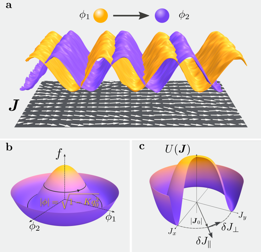
Figure 1: Emergent polar order in active scalar mixtures. (a) Due to non-reciprocal interactions, type-1 particles chase type-2 particles, while both being governed by conserved dynamics. The corresponding concentrations $\phi_{1}$ and $\phi_{2}$ exhibit phase-shifted spatio-temporal oscillations that we map onto the active polar order parameter $\boldsymbol{J}$. The corresponding configuration for the polar field $\boldsymbol{J}$ is shown in the plane below the waves. The vector fields and the waves are evaluated from numerical simulations of Eq. (1) (see Methods). (b) Representation of the free-energy density in the $(\phi_{1},\phi_{2})$ space. The wave state with amplitude $|\phi|=\sqrt{1-Kq_{0}^{2}}$ corresponds to an energetic level higher than the bottom of the potential well. (c) The ordered state $\boldsymbol{J}_{0}$ is the ground state of the Mexican-hat potential $U({\boldsymbol{J}})$, and we study the longitudinal fluctuations, $\delta J_{\parallel}$, and the perpendicular fluctuations, $\delta J_{\perp}$.

Travelling bands. The above form of NRCH model admits solutions in the form of travelling density waves (Fig. 1a), which can be represented via a complex field defined as $\phi\equiv\phi_{1}+i\phi_{2}=|\phi|\,e^{i\left({\boldsymbol{q}}_{0}\cdot\boldsymbol{x}-\omega_{0}t\right)}$, with $|\phi|=\sqrt{1-Kq_{0}^{2}}$ and $\omega_{0}=\alpha q_{0}^{2}$. The solution is stable, and is associated with a cyclic orbit in the configuration space at any point $\boldsymbol{x}$ that does not reside at the bottom of the free energy landscape, corresponding to $f=-\frac{1}{4}\left(1-K^{2}q_{0}^{4}\right)$ and $\frac{K}{2}(\boldsymbol{\nabla}\phi)^{2}+f=-\frac{1}{4}\left(1-Kq_{0}^{2}\right)^{2}$ (see Fig. 1b). In these solutions, parity and time-reversal symmetries, together with time- and space-translation symmetries are spontaneously broken. Moreover, an emergent polar order is observed in the system that is composed of two scalar fields.

Polar order parameter. To understand the nature of the emergent polar order, we start by defining a local polar order parameter $\boldsymbol{J}=\varepsilon_{ab}\phi_{a}\boldsymbol{\nabla}\phi_{b}$, which is nonzero when the density waves have a phase difference, leading to parity symmetry breaking. Using numerical simulations, it has been shown that $\boldsymbol{J}$ transitions to taking non-vanishing values when $\alpha$ is tuned to exceed the coefficient of linear reciprocal interaction [20], which is set to zero here for simplicity.

We derive the effective governing equation for the emergent polar order parameter $\boldsymbol{J}(\boldsymbol{x},t)$, using the dynamical equations for the two concentrations (1). To the leading order, we obtain

$$\partial_{t}\boldsymbol{J}+\lambda_{1}\boldsymbol{J}(\boldsymbol{\nabla}\cdot\boldsymbol{J})+\lambda_{2}(\boldsymbol{J}\cdot\boldsymbol{\nabla}){\boldsymbol{J}}=\Gamma\boldsymbol{\nabla}(\boldsymbol{\nabla}\cdot\boldsymbol{J})$$

$$+D_{lJ}\boldsymbol{J}(\boldsymbol{J}\cdot\boldsymbol{\nabla})(\boldsymbol{\nabla}\cdot\boldsymbol{J})+D_{mJ}\boldsymbol{J}\nabla^{2}|\boldsymbol{J}|^{2}+r_{1}\boldsymbol{J}$$

$$+\left(r-u|\boldsymbol{J}|^{2}\right)|\boldsymbol{J}|^{2}\boldsymbol{J}-\boldsymbol{\nabla}P+\lambda_{3}\boldsymbol{J}(\boldsymbol{J}\cdot\boldsymbol{\nabla})\rho+{\boldsymbol{\xi}}_{J},$$ (2)

where the different terms are organized such that the similarities to the Toner-Tu equations [30] are highlighted. The quantities that are introduced in Eq. (2) are functions of the amplitude $\rho(\boldsymbol{x},t)=\sqrt{\phi_{a}\phi_{a}}$, which for the traveling band solution will represent a uniform field with $\rho(\boldsymbol{x},t)=\rho_{0}=\sqrt{1-Kq_{0}^{2}}$. To the lowest order, we find $\lambda_{1}=2\alpha/\rho^{2}$, $\lambda_{2}=2\alpha/\rho^{2}$, $\Gamma=1-\rho^{2}-2m$, $D_{lJ}=4K/\rho^{4}$, $D_{mJ}=2K/\rho^{4}$, $r_{1}=2(2m+5\rho^{2}-3)\nabla^{2}\rho/\rho$, $r=2(1-\rho^{2})/\rho^{4}$, $u=2K/\rho^{8}$, $P=2\,\boldsymbol{J}\cdot\boldsymbol{\nabla}m$, $\lambda_{3}=4\alpha/\rho^{3}$. Here, we have defined the auxiliary field $m=\rho^{4}(r-u|\boldsymbol{J}|^{2})/2$, which identically vanishes in the broken symmetry state. The noise term ${\boldsymbol{\xi}}_{J}$ will be discussed below.

We can make a number of observations from Eq. (2), which describes the collective dynamics of the emergent polar order parameter field. The coefficients of the symmetry-breaking advective terms, namely $\lambda_{1}$ and $\lambda_{2}$, are proportional to $\alpha$. It is thus evident that $\alpha$ assumes the role of the velocity of self-propulsion in the Toner-Tu description and breaks Galilean invariance [30]. The deterministic dynamics of $\boldsymbol{J}$ is not conserved; this is due to a dissipative force that can be expressed as the derivative of a Mexican hat potential $U(\boldsymbol{J})=-\frac{r}{4}|\boldsymbol{J}|^{4}+\frac{u}{6}|\boldsymbol{J}|^{6}$ (see Fig. 1c), namely, $-\partial U(\boldsymbol{J})/\partial\boldsymbol{J}=(r-u|\boldsymbol{J}|^{2})\boldsymbol{J}|\boldsymbol{J}|^{2}$. For a uniform background amplitude $\rho_{0}$, the dissipative force vanishes at the steady-state value of $J_{0}=|\boldsymbol{J}_{0}|=\sqrt{r_{0}/u_{0}}$ when $r_{0}>0$ (Fig. 1c), with $r_{0}=r(\rho_{0})=2(1-\rho_{0}^{2})/\rho_{0}^{4}$ and $u_{0}=u(\rho_{0})=2K/\rho_{0}^{8}$, namely, $J_{0}=\rho_{0}^{2}\sqrt{(1-\rho_{0}^{2})/K}$. (Throughout the paper, the subscript $0$ always indicates that the quantity is evaluated at the background solution $\rho_{0}$). If we take the uniform amplitude state to represent the stable traveling band solution, then $J_{0}=\rho_{0}^{2}q_{0}$. In dimensions $d>1$, this potential is characterised by rotational symmetry, which is broken when the ground state $\boldsymbol{J}_{0}=J_{0}{\hat{\boldsymbol{e}}}$ spontaneously chooses a specific direction along ${\hat{\boldsymbol{e}}}$.

To complete the effective description of the dynamics, we need a governing equation for the amplitude, which plays the role of the density in the Toner-Tu analogy. We find

$$\partial_{t}\rho+\lambda_{4}(\boldsymbol{\nabla}\cdot\boldsymbol{J})=\beta m|\boldsymbol{J}|^{2}+D_{\rho}\nabla^{2}\rho$$

$$+\kappa\nabla^{2}|\boldsymbol{J}|^{2}+w(\boldsymbol{J}\cdot\nabla)(\nabla\cdot\boldsymbol{J})+\xi_{\rho},$$ (3)

with the coefficients given as $\lambda_{4}=\alpha/\rho$, $\beta=1/\rho^{3}$, $D_{\rho}=5-3\rho^{2}+2m$, $\kappa=K/\rho^{3}$, $w=2K/\rho^{3}$, and the noise term $\xi_{\rho}$ will be discussed below. We observe that the amplitude equation exhibits significant differences with both the conserved [30] and the non-conserved [31] versions of Toner-Tu equations.

The noise terms $\boldsymbol{\xi}_{J}$ and $\xi_{\rho}$ can be derived straightforwardly from the stochastic sources of Eq. (1), leading to

$$\begin{gathered}\boldsymbol{\xi}_{J}=\sqrt{2\mathcal{D}}\varepsilon_{ab}(\phi_{a}\boldsymbol{\nabla}-\boldsymbol{\nabla}\phi_{a})(\boldsymbol{\nabla}\cdot\boldsymbol{\xi}_{b}),\\ \xi_{\rho}=\sqrt{2\mathcal{D}}(\phi_{a}/\rho)(\boldsymbol{\nabla}\cdot\boldsymbol{\xi}_{a}),\end{gathered}$$ (4)

which are multiplicative noises and have the potential to be conserved, in apparent contradistinction to the non-conserved noise in Toner-Tu equations [30]. When we evaluate the noise terms using the traveling band solution, we obtain effective Gaussian noises with zero mean and the following correlators in Fourier space

$$\begin{gathered}\langle\xi_{J_{\perp}i}(\boldsymbol{q},\omega)\xi_{J_{\perp}j}(\boldsymbol{q}^{\prime},\omega^{\prime})\rangle=2\mathcal{D}\rho_{0}^{2}q_{0}^{2}q_{\perp i}q_{\perp j}\,\delta_{\boldsymbol{q}+\boldsymbol{q}^{\prime}}\delta_{\omega+\omega^{\prime}},\\ \langle\xi_{J_{\parallel}}(\boldsymbol{q},\omega)\xi_{J_{\parallel}}(\boldsymbol{q}^{\prime},\omega^{\prime})\rangle=8\mathcal{D}\rho_{0}^{2}q_{0}^{4}\,\delta_{\boldsymbol{q}+\boldsymbol{q}^{\prime}}\delta_{\omega+\omega^{\prime}},\\ \langle\xi_{\rho}(\boldsymbol{q},\omega)\xi_{\rho}(\boldsymbol{q}^{\prime},\omega^{\prime})\rangle=2\mathcal{D}q_{0}^{2}\,\delta_{\boldsymbol{q}+\boldsymbol{q}^{\prime}}\delta_{\omega+\omega^{\prime}}\\ \langle\xi_{\rho}(\boldsymbol{q},\omega)\xi_{J_{\parallel}}(\boldsymbol{q}^{\prime},\omega^{\prime})\rangle=4\mathcal{D}\rho_{0}q_{0}^{3}\,\delta_{\boldsymbol{q}+\boldsymbol{q}^{\prime}}\delta_{\omega+\omega^{\prime}},\end{gathered}$$ (9)

to the lowest order, where ${\boldsymbol{q}}_{\perp}={\boldsymbol{q}}-({\boldsymbol{q}}\cdot{\hat{\boldsymbol{e}}}){\hat{\boldsymbol{e}}}$ and the short-hands $\delta_{\boldsymbol{q}+\boldsymbol{q}^{\prime}}\equiv(2\pi)^{d}\delta^{d}(\boldsymbol{q}+\boldsymbol{q}^{\prime})$ and $\delta_{\omega+\omega^{\prime}}\equiv(2\pi)\delta(\omega+\omega^{\prime})$ have been used. We thus observe that while the noise terms for the longitudinal emergent polar order parameter and the amplitude are non-conserved, the noise terms for the transverse emergent polar order parameter are conserved.

Linear theory. The ordered state that is predicted by Eq. (2) identifies a phase separated state with spatial modulation, as well as spontaneous breaking of time-reversal and rotational symmetry. To test the robustness of $\boldsymbol{J}_{0}$ in the presence of noise, we linearly expand Eqs. (2) and (3) around the steady-state. We substitute $\boldsymbol{J}=\boldsymbol{J}_{0}+\delta\boldsymbol{J}=(J_{0}+\delta J_{\parallel}){\hat{\boldsymbol{e}}}+\delta\boldsymbol{J}_{\perp}$ distinguishing longitudinal and perpendicular fluctuations, and perturb the amplitude as $\rho=\rho_{0}+\delta\rho$. We derive the fluctuating linear dynamics up to second order in gradients,

$$\partial_{t}\delta\rho=-2\beta_{0}q_{0}^{2}\rho_{0}^{5}\gamma^{2}\delta\rho-2\beta_{0}\Gamma_{0}J_{0}\delta J_{\parallel}-\lambda_{4,0}(\boldsymbol{\nabla}\cdot\delta\boldsymbol{J})+D_{\rho,0}\nabla^{2}\delta\rho+w_{0}J_{0}[\nabla^{2}\delta J_{\parallel}+\partial_{\parallel}(\boldsymbol{\nabla}\cdot\delta\boldsymbol{J})]+{\xi}_{\rho},$$ (10)

$$\partial_{t}\delta J_{\parallel}=-4q_{0}^{2}\Gamma_{0}\delta J_{\parallel}-4q_{0}^{3}\rho_{0}^{3}\gamma^{2}\delta\rho-2J_{0}\lambda_{1,0}(\partial_{\parallel}\delta J_{\parallel})-J_{0}\lambda_{1,0}(\boldsymbol{\nabla}_{\perp}\cdot\delta\boldsymbol{J}_{\perp})+J_{0}^{2}\lambda_{3,0}\partial_{\parallel}\delta\rho+2q_{0}\rho_{0}D_{\rho,0}\nabla_{\perp}^{2}\delta\rho$$ (11)

$$\qquad+2q_{0}\rho_{0}(D_{\rho,0}+\rho_{0}^{2}\gamma^{2})\partial_{\parallel}^{2}\delta\rho+13\Gamma_{0}(\partial_{\parallel}^{2}\delta J_{\parallel})+4\Gamma_{0}\nabla_{\perp}^{2}\delta J_{\parallel}+5\Gamma_{0}\partial_{\parallel}(\boldsymbol{\nabla}_{\perp}\cdot\delta\boldsymbol{J}_{\perp})+{\xi}_{J_{\parallel}},$$

$$\partial_{t}\delta\boldsymbol{J}_{\perp}=-\lambda_{2,0}J_{0}\partial_{\parallel}\delta\boldsymbol{J}_{\perp}+4q_{0}\rho_{0}^{3}\gamma^{2}\boldsymbol{\nabla}_{\perp}\partial_{\parallel}\delta\rho+\Gamma_{0}\boldsymbol{\nabla}_{\perp}(\boldsymbol{\nabla}_{\perp}\cdot\delta\boldsymbol{J}_{\perp})+5\Gamma_{0}\boldsymbol{\nabla}_{\perp}(\partial_{\parallel}\delta J_{\parallel})+{\boldsymbol{\xi}}_{J_{\perp}},$$ (12)

where we have used $\partial_{\parallel}\equiv{\hat{\boldsymbol{e}}}\cdot\boldsymbol{\nabla}$, $\boldsymbol{\nabla}_{\perp}\equiv\boldsymbol{\nabla}-{\hat{\boldsymbol{e}}}({\hat{\boldsymbol{e}}}\cdot\boldsymbol{\nabla})$, and $\gamma^{2}=(3\rho_{0}^{2}-2)/\rho_{0}^{2}$.

The slow modes. From Eq. (12), the fluctuations that are perpendicular to the broken symmetry direction, $\delta\boldsymbol{J}_{\perp}$, can be identified as slow modes of the model, as they represent the Goldstone modes associated with the continuous rotational symmetry breaking (Fig 1). While $\delta\rho$ and $\delta J_{\parallel}$ appear to be fast variables, the existence of a constraint in the form of a curl-free condition $\partial_{i}(J_{j}/\rho^{2})-\partial_{j}(J_{i}/\rho^{2})=0$ suggests that an additional slow mode that combines the two fields also exists in the dynamics. Examining the eigen-mode structure of Eqs. (10) and (11), we identify the new slow variable as $\delta s=\delta J_{\parallel}-2(J_{0}/\rho_{0})\delta\rho$. Solving for different linear slow modes, we find

$$\delta{\boldsymbol{J}}_{\perp}(\boldsymbol{q},\omega)={\cal G}(\boldsymbol{q},\omega)\,{\boldsymbol{\xi}}_{J_{\perp}}(\boldsymbol{q},\omega),$$ (13)

$$\delta s(\boldsymbol{q},\omega)={\cal G}(\boldsymbol{q},\omega)\,\xi_{s}(\boldsymbol{q},\omega),$$ (14)

in terms of the Green function of the linear dynamics ${\cal G}(\boldsymbol{q},\omega)=\left[i(\omega-v_{g}q_{\parallel})+\Gamma_{0}\left(q_{\perp}^{2}+\gamma^{2}q_{\parallel}^{2}\right)\right]^{-1}$. The coefficient $v_{g}=2\alpha q_{0}$ advects the fluctuations along the ordering direction and represents the propagating sound speed. The diffusion is anisotropic with coefficients $\Gamma_{0}=Kq_{0}^{2}$ along the transverse directions and $\Gamma_{0}\gamma^{2}=Kq_{0}^{2}(3\rho_{0}^{2}-2)/\rho_{0}^{2}$ along the longitudinal direction. Note that the stability of the dynamics requires $\rho_{0}^{2}>2/3$ (in order to have $\gamma^{2}>0$), which is connected to the Eckhaus instability [38]. The noise for the new slow mode in Eq. (14) has zero mean and the following correlator

$$\langle\xi_{s}(\boldsymbol{q},\omega)\xi_{s}(\boldsymbol{q}^{\prime},\omega^{\prime})\rangle=2\mathcal{D}\rho_{0}^{2}q_{0}^{2}q_{\parallel}^{2}\,\delta_{\boldsymbol{q}+\boldsymbol{q}^{\prime}}\delta_{\omega+\omega^{\prime}}.$$ (15)

We note that the dynamics of the slow modes corresponds to a rather uncommon class where the deterministic evolution of the dynamics is dissipative while the noise contribution that drives the stochastic fluctuations is conserved [39].

Long-Range Oder in $d>1$. We can now calculate the magnitude of the transverse fluctuations of the emergent polar order parameter. Combining Eqs. (13) and (9), we have $\langle|\delta\boldsymbol{J}_{\perp}(\boldsymbol{x},t)|^{2}\rangle=\int_{\omega}\int^{\Lambda}_{\boldsymbol{q}}2\mathcal{D}\rho_{0}^{2}q_{0}^{2}q_{\perp}^{2}|{\cal G}(\boldsymbol{q},\omega)|^{2}$ with $\Lambda$ being the finite ultraviolet cutoff. The integrals can be calculated to give

$$\langle|\delta\boldsymbol{J}_{\perp}(\boldsymbol{x},t)|^{2}\rangle=(d-1)\frac{\mathcal{D}\rho_{0}^{2}}{dK}\frac{\Lambda^{d}}{(2\pi)^{d}},$$ (16)

which stays finite below the onset of Eckhaus instability for any $d>1$. Therefore, in our theory transverse fluctuations are suppressed and the system exhibits true long-range order in $\boldsymbol{J}$ for any $d>1$ even at the linear level.

Non-linear theory. To verify to which extent the predictions of linear theory hold, we need to understand the role of non-linearities. The most relevant contributions are given by terms containing one gradient and two fields, coupling the dynamics of transverse and longitudinal slow modes. Below, we will show that these are the solely relevant nonlinear term as predicted by the Renormalization Group framework. After expanding Eqs. (2) and (3) at this order in fluctuations, changing to the comoving frame of reference (with velocity $v_{g}\,{\hat{\boldsymbol{e}}}$), and rescaling the longitudinal coordinate by $\gamma$, we can write down the dynamics for a vector field $\boldsymbol{p}=\gamma\,\delta s\,{\hat{\boldsymbol{e}}}+\delta\boldsymbol{J}_{\perp}$, as follows

$$\partial_{t}\boldsymbol{p}+\lambda_{0}\boldsymbol{p}\cdot\boldsymbol{\nabla}\boldsymbol{p}=\Gamma_{0}\nabla^{2}\boldsymbol{p}-\boldsymbol{\nabla}\eta(\boldsymbol{x},t),$$ (17)

where the nonlinear coupling constant can be traced back to the non-reciprocity as $\lambda_{0}=2\alpha/\rho_{0}^{2}$, and we have used the curl-free condition reported above as inherited by $\boldsymbol{p}$, namely $\partial_{i}p_{j}-\partial_{j}p_{i}=0$. The variance of the noise reads $\langle\eta(\boldsymbol{q},\omega)\eta(\boldsymbol{q}^{\prime},\omega^{\prime})\rangle=2D_{0}\,\delta_{\boldsymbol{q}+\boldsymbol{q}^{\prime}}\delta_{\omega+\omega^{\prime}}$, where the amplitude is given as $D_{0}=\mathcal{D}q_{0}^{2}\rho_{0}^{2}\gamma$. Remarkably, we thus obtain the well-known noisy Burgers equation [34, 40].

We finally express the polar vector field as the gradient of a scalar function $\boldsymbol{p}=-\boldsymbol{\nabla}h$, as the curl-free constraint implies. The dynamics (17) thus becomes

$$\partial_{t}h=\Gamma_{0}\nabla^{2}h+\frac{\lambda_{0}}{2}(\nabla h)^{2}+\eta(\boldsymbol{x},t),$$ (18)

namely, the celebrated Kardar-Parisi-Zhang (KPZ) equation in any dimension $d$ [33]. This result states that the non-linear dynamics of the fluctuating modes around the ordered traveling state of our system can be mapped to the equation for growing interfaces described by the height function $h(\boldsymbol{x},t)$, thus belonging to its universality class. Non-reciprocity, here described by the parameter $\alpha$, is the key ingredient to connect the NRCH model for particle densities to the KPZ equation. We note that the KPZ field represents the fluctuations of the constant phase manifolds in the underlying complex field theory involving the order parameter $\phi=\rho\,e^{i\theta}$, namely, $\theta(\boldsymbol{x},t)=\gamma{\boldsymbol{q}}_{0}\cdot\boldsymbol{x}-(\omega_{0}-v_{g}q_{0})t-h(\boldsymbol{x},t)$ in terms of the new coordinates. Therefore, the flatness or roughness of the KPZ field can be interpreted as a reflection on the shape of the bands in the NRCH model, which effectively represents an active traveling smectic phase [20].

Renormalization Group predictions. We can now use the results on the critical dynamics of the KPZ equation to characterize the scaling behavior of our emergent polar order parameter. For a scaling factor $b=e^{l}\gtrsim 1$, we will seek to find scaling transformations in the form of as $t\to b^{z}t,\ \boldsymbol{x}\to b\boldsymbol{x},\ \boldsymbol{p}\to b^{\zeta-1}\boldsymbol{p}$ such that the dynamics (17) is scale invariant. Here, $z$ is the dynamical critical exponent, and $\zeta$ is the roughness exponent of the underlying KPZ field $h$. Applying these transformations to Eq. (17), we obtain the following scaling relations for the coupling constants of the field theory: $\Gamma_{b}=\Gamma_{0}b^{z-2}$, $D_{b}=D_{0}b^{z-d-2\zeta}$, and $\lambda_{b}=\lambda_{0}b^{\zeta+z-2}$. The Gaussian fixed point corresponds to $\lambda^{*}=0$ at which the long-wavelength dynamics is ruled by the linear theory with exponents $z=2$ and $\zeta=1-d/2$. These exponents determine the critical dimension $d_{c}=2$ at which the non-linearity $\lambda_{0}$ is only marginally relevant. With these scaling dimensions, it is easy to verify that all higher order non-linearities are irrelevant.

Perturbative Renormalization Group calculations performed for the effective coupling constant of theory $g=K_{d}\,{\lambda_{0}^{2}D_{0}}/{\left(4\Gamma_{0}^{3}\right)}$ (in which $K_{d}\equiv{S_{d}}/{(2\pi)^{d}})$ and $S_{d}=2\pi^{d/2}/\Gamma(d/2)$ is the area of the unit-sphere in $d$ dimensions) yields

$$\frac{{\rm d}g}{{\rm d}l}=(2-d)g+\frac{2}{d}\left(2d-3\right)g^{2},$$ (19)

at one-loop order [40]. For $d=1$, Eq. (19) suggests that the dynamics is governed by a stable fixed point at $g^{*}=1/2$ (with the fixed point at $g^{*}=0$ being unstable), which corresponds to exponents $\zeta=1/2$ and $z=3/2$ that turn out to be exact. At $d=2$, the fixed point at $g^{*}=0$ is marginally unstable, which hints at the existence of a correlation length given as

$$\ell_{\times}=\frac{2\pi}{q_{0}}\exp\left(\frac{2\pi K^{3}q_{0}^{4}}{\gamma\alpha^{2}\mathcal{D}}\right).$$ (20)

For length scales smaller than $\ell_{\times}$, the dynamics is governed by the $g^{*}=0$ fixed point that corresponds to $\zeta=0$ and $z=2$, whereas for length scales larger than $\ell_{\times}$ a strong coupling fixed point controls the dynamics. For $d=3$, an unstable fixed point $g^{*}=1/2$ separates two phases: a flat phase characterized by the stable fixed point $g^{*}=0$ corresponding to $\alpha<\alpha_{c}$, and a rough phase controlled by a strong coupling fixed point corresponding to $\alpha>\alpha_{c}$. The onset of the roughening transition occurs at

$$\alpha_{c}=\left(\frac{\pi^{2}K^{3}q_{0}^{4}}{\gamma\mathcal{D}}\right)^{1/2}.$$ (21)

Calculations up to two-loop order (that introduce higher order terms in Eq. (19)) do not significantly change the above conclusions [41, 42]. Note that NRCH provides a unique opportunity for an experimental realization of the 3D KPZ universality class, and the corresponding roughening transition, without the need to have access to 4D position space.

It is important to examine how the question of true long-range emergent polar order is influenced by the presence of nonlinearity in the dynamics, and how it is affected by whether the constant-$\theta$ bands are statistically flat or rough. The fluctuations in the polarization can be calculated as

$$\langle{\boldsymbol{p}}(\boldsymbol{x},t)^{2}\rangle=\langle{\boldsymbol{\nabla}}h(\boldsymbol{x},t)^{2}\rangle\sim\int_{1/L}^{\Lambda}q^{1-2\zeta}dq\sim\Lambda^{2(1-\zeta)},$$ (22)

which is finite as long as $\zeta<1$ holds; note that Eq. (22) would yield $\sim L^{2(\zeta-1)}$ when $\zeta>1$, which would diverge with the system size $L$. Inserting the Gaussian fixed point value of $\zeta=1-d/2$ in Eq. (22) yields $\Lambda^{d}$, which is the result reported in Eq. (16). It is, indeed, known that $\zeta<1$ generally holds for KPZ equation in any dimension, with the most recent conjecture of $\zeta=7/(4d+10)$ (and, correspondingly, $z=\frac{8d+13}{4d+10}$) representing well the numerically obtained results so far [43]. Therefore, the true long-range order in the emergent polar order parameter persists even in the presence of the nonlinear term and when the underlying KPZ dynamics is governed by the perturbatively inaccessible strong coupling fixed point, e.g. in $d=2$ and beyond the roughening transition (corresponding to $\alpha>\alpha_{c}$) in $d=3$.

Discussion and conclusions. We present a new effective theory for a mixture of two species with non-reciprocal interaction as described by conserved scalar fields, in terms of an emergent polar order parameter field that breaks time-reversal symmetry. Our framework shows striking similarities with the Toner-Tu theory of dry polar active matter, most notably an ordering potential and nonlinearities describing activity-driven advection. The effective theoretical framework for the emergent polar order parameter field predicts rotational symmetry breaking and the existence of Goldstone modes that emerge as a result of broken rotational symmetry. The theory, however, features marked differences with the Toner-Tu theory. The amplitude equation is not equivalent either to the conserved [30] or the Malthusian [31] versions of Toner-Tu equations. Moreover, the noise that drives the soft modes is conserved, which leads to a violation of the Mermin-Wagner theorem in $d=2$ [44], already at the linear level, as the low-cost and thus easily excitable elastic deformations of the Goldstone modes are suppressed by the vanishing strength of the spontaneous fluctuations at the largest length scales. We note that most existing theories of polar active matter do not show long-range order in $d=2$ at the linear level, and non-linear active terms are necessary to tame fluctuations around the ordered state [3], with the exception of theories that incorporate a momentum conserving fluid near a boundary [13, 45, 46].

The predictions of the linear theory are validated by our analysis including nonlinear terms. We show that the fluctuating modes of our theory follow a noisy Burgers equation for a single curl-free vectorial field, which can be mapped to a KPZ dynamics in every $d$. We observe that the relevant nonlinearity is produced by non-reciprocity and cannot generate any non-conserved noise term under renormalization. Building on the effective KPZ description of the fully nonlinear theory, we prove that the system exhibits true long-range polar order in any dimension, which is the central result of our work.

We would like to close by highlighting an important feature of the emergent polar order parameter, which can be written as $\boldsymbol{J}=\frac{1}{2i}\left(\phi^{*}\boldsymbol{\nabla}\phi-\phi\boldsymbol{\nabla}\phi^{*}\right)$ in analogy to quantum mechanics: it has been constructed to measure the coherence between the two species in the NRCH model. In light of this definition, one can argue that investigating the dynamics of $\boldsymbol{J}$ follows the same spirit as studying the effective dynamics of composite particles in quantum condensed matter systems [5, 6]. Moreover, since coherence is the interesting physical observable, $\phi$ plays a role that is more analogous to a wave function than a density, whereas $\rho^{2}$ plays the role of density or probability, again, highlighting the significance of the composite particles that chase each other taking on the role of the fundamental unit of the effective theory, leading to the emergence of an unanticipated polar symmetry.

Appendix

Numerical Simulations. Simulations shown in Fig. 1a have been performed using a pseudo-spectral method with periodic boundary conditions. The algorithm combines the evaluation of linear terms in Fourier space and non-linear terms in real space in order to obtain a stable solution of the non-linear partial differential equations (PDE)s; more details can be found in Ref. [20]. Initial conditions have been chosen as waves with minimum wave-number $q_{\rm min}=2\pi/L$, as perturbed with a white Gaussian noise extracted independently on each lattice-site. We use a forward Euler-Maruyama method to perform the time integration [47]. The noise fields were generated at each point of the lattice and each time-step from a Gaussian distribution with zero mean and unit width.

Noise for the slow mode dynamics. Equation (4) represents the noise corresponding to the polar order parameter and the amplitude, as derived from the conserved additive noise of Eq. (1). Here, we do not consider spurious drifts in the dynamics of these fields [48]. In order to determine the relevant noise contributions to the linear dynamics of $\delta\rho$ and $\delta\boldsymbol{J}$, we expand the conserved multiplicative noise of Eq. (4) around the traveling wave state $\phi_{a}=\bar{\phi}_{a}(\boldsymbol{x},t)+\delta\phi_{a}(\boldsymbol{x},t)$, with $\bar{\phi}_{1}=\rho_{0}\cos\theta_{0}(\boldsymbol{x},t)$ and $\bar{\phi}_{2}=\rho_{0}\sin\theta_{0}(\boldsymbol{x},t)$. For fluctuations of the polar order parameter we obtain

$$\boldsymbol{\xi}_{J}=\sqrt{2\mathcal{D}}[\varepsilon_{ab}\boldsymbol{\nabla}\bar{\phi}_{b}\boldsymbol{\nabla}\cdot\boldsymbol{\xi}_{a}+\varepsilon_{ab}\bar{\phi}_{a}\boldsymbol{\nabla}(\boldsymbol{\nabla}\cdot\boldsymbol{\xi}_{b})],$$

which we can subsequently project onto the perpendicular and longitudinal directions, as follows

$$\xi_{J_{\parallel}}=\sqrt{2\mathcal{D}}[\varepsilon_{ab}(\partial_{\parallel}\bar{\phi}_{b})\boldsymbol{\nabla}\cdot\boldsymbol{\xi}_{j}+\varepsilon_{ab}\bar{\phi}_{a}\partial_{\parallel}(\boldsymbol{\nabla}\cdot\boldsymbol{\xi}_{j})],$$

$$\boldsymbol{\xi}_{J_{\perp}}=\sqrt{2\mathcal{D}}\varepsilon_{ab}\bar{\phi_{a}}\boldsymbol{\nabla}_{\perp}(\boldsymbol{\nabla}\cdot\boldsymbol{\xi}_{b}),$$

while for the amplitude fluctuations we obtain

$$\xi_{\rho}=\sqrt{2\mathcal{D}}(\bar{\phi}_{a}/\rho_{0})\boldsymbol{\nabla}\cdot\boldsymbol{\xi}_{a}.$$

In Fourier space, the main effect of the spatio-temporal oscillations is to translate wave-number and frequency by the selected $q_{0}$ and $\omega_{0}$. Mean values are null, and the variances for the longitudinal fast fields become,

$$\langle\xi_{\rho}(\boldsymbol{q},\omega)\xi_{\rho}(\boldsymbol{q}^{\prime},\omega^{\prime})\rangle=2\mathcal{D}(q_{0}^{2}+q^{2})\delta_{\boldsymbol{q}+\boldsymbol{q}^{\prime}}\delta_{\omega+\omega^{\prime}},$$

$$\langle\xi_{J\parallel}(\boldsymbol{q},\omega)\xi_{J\parallel}(\boldsymbol{q}^{\prime},\omega^{\prime})\rangle=8\mathcal{D}\rho_{0}^{2}q_{0}^{4}\delta_{\boldsymbol{q}+\boldsymbol{q}^{\prime}}\delta_{\omega+\omega^{\prime}}+$$

$$+2\mathcal{D}\rho_{0}^{2}q_{0}^{2}(4q^{2}+9q_{\parallel}^{2}+q^{2}q_{\parallel}^{2}/q_{0}^{2})\delta_{\boldsymbol{q}+\boldsymbol{q}^{\prime}}\delta_{\omega+\omega^{\prime}},$$

We note that the leading contributions are non-conserved. However, they cancel in the definition of $\delta s$ producing conserved noise for the longitudinal and transverse slow modes:

$$\langle\xi_{s}(\boldsymbol{q},\omega)\xi_{s}(\boldsymbol{q}^{\prime},\omega^{\prime})\rangle=2\mathcal{D}\rho_{0}^{2}q_{\parallel}^{2}(q_{0}^{2}+q^{2})\delta_{\boldsymbol{q}+\boldsymbol{q}^{\prime}}\delta_{\omega+\omega^{\prime}},$$

$$\langle\xi_{J_{\perp}i}(\boldsymbol{q},\omega)\xi_{J_{\perp}j}(\boldsymbol{q}^{\prime},\omega^{\prime})\rangle=2\mathcal{D}\rho_{0}^{2}q_{\perp i}q_{\perp j}\left(q_{0}^{2}+q^{2}\right)\delta_{\boldsymbol{q}+\boldsymbol{q}^{\prime}}\delta_{\omega+\omega^{\prime}}.$$

At the leading order, these are conserved additive noise terms with amplitudes of order $\sim q^{2}$. At large momenta the conservation law produces an order $\sim q^{4}$ behaviour.