PAT: Pixel-wise Adaptive Training for Long-tailed Segmentation

Abstract

Beyond class frequency, we recognize the impact of class-wise relationships among various class-specific predictions and the imbalance in label masks on long-tailed segmentation learning. To address these challenges, we propose an innovative Pixel-wise Adaptive Training (PAT) technique tailored for long-tailed segmentation. PAT has two key features: 1) class-wise gradient magnitude homogenization, and 2) pixel-wise class-specific loss adaptation (PCLA). First, the class-wise gradient magnitude homogenization helps alleviate the imbalance among label masks by ensuring equal consideration of the class-wise impact on model updates. Second, PCLA tackles the detrimental impact of both rare classes within the long-tailed distribution and inaccurate predictions from previous training stages by encouraging learning classes with low prediction confidence and guarding against forgetting classes with high confidence. This combined approach fosters robust learning while preventing the model from forgetting previously learned knowledge. PAT exhibits significant performance improvements, surpassing the current state-of-the-art by $2.2\%$ in the NyU dataset. Moreover, it enhances overall pixel-wise accuracy by $2.85\%$ and intersection over union value by $2.07\%$, with a particularly notable declination of $0.39\%$ in detecting rare classes compared to Balance Logits Variation, as demonstrated on the three popular datasets, i.e., OxfordPetIII, CityScape, and NYU. The code will be released upon acceptance.

1 Introduction

The integration of deep learning (DL) into real-world applications has sparked fresh enthusiasm for research extending beyond meticulously crafted datasets with balanced classes and accurate representations of the test set distribution. However, it is doubtful to foresee and construct datasets that encompass all potential scenarios consistently. Therefore, it is crucial to explore robust algorithms that can perform well on imbalanced datasets and unforeseen circumstances during testing. These challenges can be classified as distributional shifts between the training and testing conditions, notably, label prior shift and non-semantic likelihood shift [8].

Many researchers attempt to propose robust algorithms against long-tailed rare categories in segmentation via resampling [3, 7], data augmentation [26, 20], logits adjustment (LA) [9, 1, 24, 12, 27], domain adaptation (DA) [30, 11, 29]. However, the imbalance among classes inside samples in segmentation remains a critical issue. Existing efforts predominantly concentrate on addressing sample imbalance within classes, with limited research devoted to long-tailed segmentation. The data augmentation and sampling method prove inadequate as it can neither augment nor sample classes within masks. Additionally, designing model architectures for this purpose is highly resource-intensive and computationally demanding.

Recognizing these challenges, we delve into existing research on long-tailed segmentation and uncover intriguing insights. 1) Imbalanced mask representations: beyond the difficulties posed by rare objects, imbalanced mask representations occur when some masks dominate the learning process, leading to a bias towards recognizing dominant classes and neglecting minority classes. 2) Model uncertainty and degradation: models facing uncertainty often produce low-precision channel-wise logits, leading to biased gradient updates. These updates favor incorrect label predictions and ignore progress toward the true labels, further degrading performance.

Building upon these insights, we introduce Pixel-wise Adaptive Training (PAT), a novel approach for addressing long-tailed rare category problems in segmentation. PAT comprises two key contributions: 1) Class-wise Gradient Magnitude Homogenization: We address the imbalanced learning caused by differences in object size across classes by dividing the loss by the corresponding class mask’s size. This effectively equalizes the influence of each class on the learning process. 2) Pixel-wise Class-Specific Loss Adaptation (PCLA): This component focuses on pixel-wise predicting vectors (PPVs) within each pixel (see Fig. 3(a)). By examining the PPVs, we can evaluate how individual channels influence the learning process by analyzing the logit predictions. Specifically, by employing an inverted softmax function, we can strike a balance between two factors: the presence of long-tailed rare objects and the impact of insufficient loss contribution on the joint loss function. This equilibrium enables us to determine coefficients that prioritize learning in classes with rare objects or those with minimal contributions to the joint loss induced by the wrong predictions of the model from previous low-performance learning progress. Consequently, we address the issue of imbalanced learning stemming from both current training samples and previously learned imbalances in the models.

2 Related Works

2.1 LongTailed Learning in Segmentation

Several studies have explored the phenomenon of longtail distribution within segmentation contexts. Different from the traditional classification task, resampling methods [3, 7] as well as data augmentation [26, 20] cannot tackle the underlying issues of long-tail distribution in segmentation as the ratio among class frequencies is not adjusted[31]. Logits adjustment (LA) is one of the most prominent techniques that can balance the effect of head class logits by equalizing the output logits distribution [9, 1, 24, 12, 27]. Domain adaptation [30, 11, 29] is also considered to enhance the logits balancing, though accessing the target dataset is impractical in real-world applications [25]. Post-processing is useful in removing the uncertainty [18] at the pixel level in semantic segmentation, though it requires a calibration process for each dataset.

2.2 Class Sensitive Learning

Class-sensitive learning (CSL) is one direction in solving long-tailed learning [31], which takes full advantage of classes’ frequency to balance the logits distribution, class-wise gradient, etc. From Section 2.1, it turns out that LA and CSL are the two most easy-to-use yet effective methods in long-tailed learning. Focal (Focal) function [13] is firstly proposed to tackle this challenge by taking the inverse of logits as a weight for each class. In [6], a class-balance loss function is proposed, working as an effective sampler by a class frequency weighting function. The combination of class-balance loss and Focal is also considered in [6]. Balancing the effect of the exponential function in the Softmax activation function is studied [24, 12]. Other recent methods [4, 26] focus on using noise in logits to balance them which are also popular in segmentation, we also compare our proposed method with those ones. We also show that our proposed method surpasses the others in both performance and utilization.

3 Proposed Method

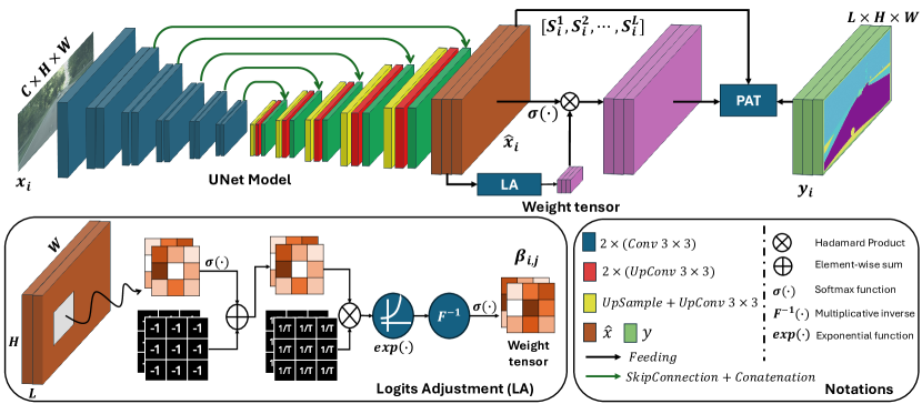
Figure 1: Overall methodology. 1) Training procedure: an input image $x_{i}$ is fed into a typical encoder-decoder model architecture to produce output $\hat{x}_{i}$. This prediction’s logits are then adjusted to create a weight tensor, which has the same size as $\hat{x}_{i}$. The normalized $\hat{x}_{i}$ is multiplied by the weight tensor to balance the dominant logits. Finally, the loss value is obtained using the proposed PAT loss function. 2) Logits Adjustment: The logits vector is normalized by the Softmax function, added by a tensor of $-1$, and scaled by the exponential function to find the inverse dominant coefficients $\beta_{i,j}$. Then, these coefficients are normalized into a range of $[0,1]$ to form the weight tensor.

3.1 Problem Statement

Consider $(x,y)\sim P(\mathcal{X},\mathcal{Y})$, where $x\in\mathbb{R}^{N\times C\times H\times W}$ and $y\in\mathbb{R}^{N\times L\times H\times W}$ are input data and corresponding ground truth, respectively. $C$, $L$ are the number of image channels and categories, respectively. $N$, $H$, and $W$ are the total number of training samples, height, and width of the image, separately. The segmentation problem is represented in Eq. (1).

$$\mathcal{L}(x,y) =\frac{1}{B}\sum^{B-1}_{i=0}\sum^{L-1}_{l=0}\mathcal{L}_{l}(x_{i},y_{i}),$$ (1)

where $\mathcal{L}_{l}(x_{i},y_{i})=-\log\Big{(}\frac{\exp\{\hat{x}^{l}_{i}\}}{\sum_{l^{\prime}=0}^{L-1}\exp\{\hat{x}^{l^{\prime}}_{i}\}}\Big{)}y^{l}_{i}$ denotes the class-wise loss on sample $x_{i}\in\mathbb{R}^{C\times H\times W}$ and its corresponding ground truth $y_{i}\in\mathbb{R}^{L\times H\times W}$. $\hat{x}^{l}_{i},y^{l}_{i}\in\mathbb{R}^{H\times W}$ are the predicted mask and the ground-truth of channel $l$ (which represents class $l$), respectively.

3.2 Imbalance among label masks

One major challenge in image segmentation is the class imbalance in label masks (see Fig. 2). Larger masks contribute more significantly to the loss of function than smaller masks, leading to a bias towards dominant classes. Specifically, we come over the class-wise loss component, which can be represented as:

$$\mathcal{L}_{l}(x_{i},y_{i}) =-\sum^{HW}_{j=0}\log\Big{(}\frac{\exp\{\hat{x}^{l}_{i,j}\}}{\sum_{l^{\prime}=0}^{L-1}\exp\{\hat{x}^{l^{\prime}}_{i,j}\}}\Big{)}y^{l}_{i,j}$$ (2)

$$=-\sum^{HW}_{j=0}\log\Big{(}\frac{\exp\{\hat{x}^{l}_{i,j}\}}{\sum_{l^{\prime}=0}^{L-1}\exp\{\hat{x}^{l^{\prime}}_{i,j}\}}\Big{)}\mathbbm{I}(y^{l}_{i,j}=1)=S^{l}_{i}\times\bar{\ell}_{l}(x_{i},y_{i}),$$

where $S^{l}_{i}$ and $\bar{\ell}_{l}(x_{i},y_{i})$ denote the size of label $l$ mask and the cross-entropy value on class $l$ for image $i$, respectively, where $S^{l}_{i}=\sum^{HW}_{j=0}\mathbbm{1}(y^{l}_{i,j}=1)$.

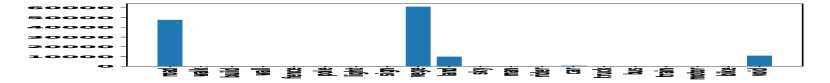
(a)

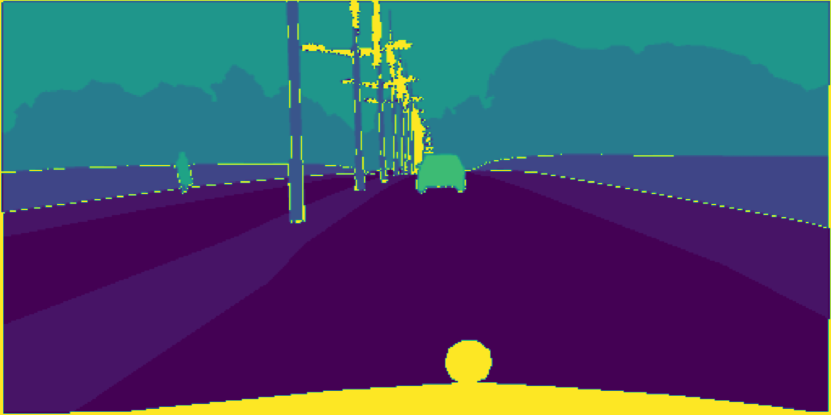
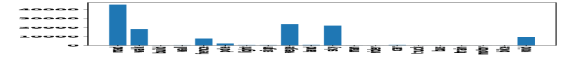
(b)

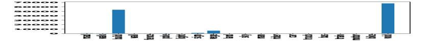
(c)

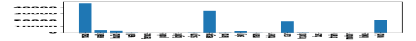
(d)

Figure 2: Quantitative analysis on the imbalance in mask size among classes. The vertical axis illustrates the mask size calculated by the total number of pixels, which are associated with the corresponding mask. The horizontal axis shows different masks that potentially appear in the ground truth. 2(a)) While road and vegetation take 50000 pixels and 60000 pixels, respectively, cars account for around 1000 pixels. 2(b)) Not only road and vegetation but also walking and sky take roughly $99\%$ proportion, compared to cars. 2(c)) Void and build take nearly 70000 pixels and 60000 pixels, under 1000 pixels are accounted by sign, and no car appears. 2(d)) Cars take roughly 20000 pixels, though their masks’ sizes are much bigger than the ones in Figs. 2(a) and 2(b).

While the traditional approach is rooted in classification problems, in segmentation tasks, the loss is adjusted based on the mask size $S^{l}_{i}$. Consequently, to ensure uniformity in gradient magnitude, we diminish the loss by the label mask size of each instance. This adjustment guarantees that all class-specific loss pixels receive equal consideration within the collective loss function.

3.3 Pixel-wise Adaptive Traning with Loss Scaling

The summary of the methodology is shown in Fig. 1. To design an adaptive pixel-wise loss scaling, we first decompose the conventional segmentation function into a pixel-wise function (refer to Eq. (3)), which is derived from Eq. (1).

$$\mathcal{L}(x,y)=-\frac{1}{B}\sum^{B-1}_{i=0}\sum^{HW}_{j=1}\Biggr{[}\sum^{L-1}_{l=0}y^{l}_{i,j}\log\Big{(}\frac{\exp\{\hat{x}^{l}_{i,j}\}}{\sum_{l^{\prime}=0}^{L-1}\exp\{\hat{x}^{l^{\prime}}_{i,j}\}}\Big{)}\Biggr{]},$$ (3)

where $\hat{x}^{l}_{i,j}$ is the logits prediction of sample $i$ at pixel $j$ with regard to category $l$. In segmentation problems, the class is considered by a composition of many pixels over the masks. We hypothesize that the learning in each class may occur diversely according to the classification of different pixels. Therefore, we propose the pixel-wise adaptive (PAT) loss via the pixel-wise adaptive coefficient set $\beta_{i,j}\in\mathbb{R}^{L}=\large[\beta_{i,j}^{0},\beta_{i,j}^{1},\cdots,\beta_{i,j}^{L-1}\large]$.

$$\mathcal{L}(x,y)=-\frac{1}{B}\sum^{B-1}_{i=0}\sum^{HW}_{j=1}\Biggr{[}\sum^{L-1}_{l=0}\beta_{i,j}^{l}\times\frac{y^{l}_{i,j}}{S^{l}_{i}}\log\Big{(}\frac{\exp\{\hat{x}^{l}_{i,j}\}}{\sum_{l^{\prime}=0}^{L-1}\exp\{\hat{x}^{l^{\prime}}_{i,j}\}}\Big{)}\Biggr{]}.$$ (4)

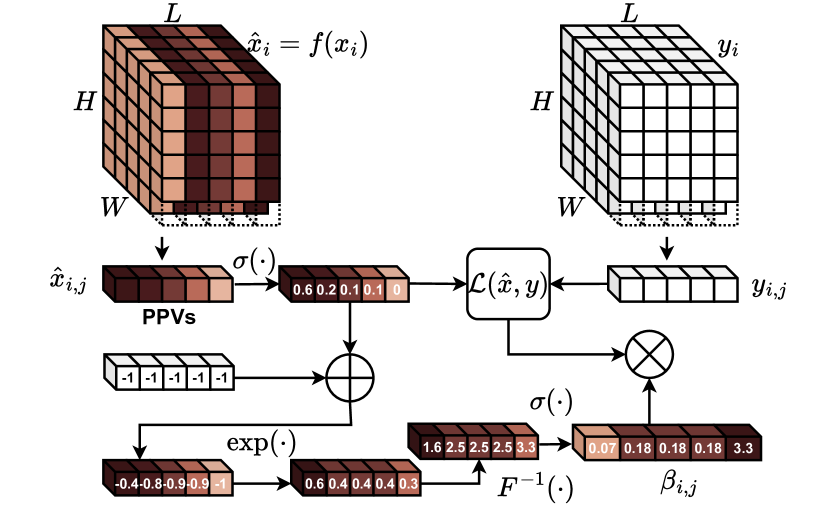
(a)

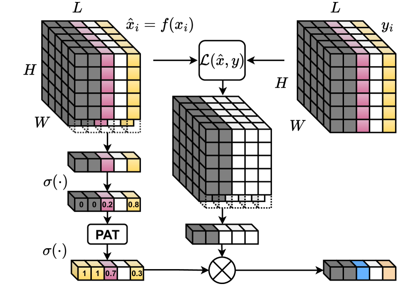
(b)

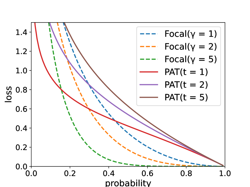
(c)

Figure 3: Fig. 3(a) illustrates the PAT procedure of adjusting the logits’ value to tackle the imbalance in dominant probability from categories whose big mask size. Fig. 3(b) shows the process of adaptive gradient scaling in PAT. Specifically, the channels with no mask can easily be adapted. Therefore, the problem of adaptive gradient scaling can be reduced to two cases. In addition to Fig. 3(a), Fig. 3(c) shows the difference in scaling coefficient between PAT and Focal[13], that PAT (smooth lines) (i) puts a higher weight on low confidence pixel and (ii) keeps low scaling coefficients for high confidence pixels. Otherwise, Focal (dash line), puts zero scalarization on well-classified pixels that may cause forgetfulness of frequent or big mask size categories.

Our key idea is to control the PAT loss using $\beta_{i,j}$. Essentially, $\beta_{i,j}$ represents a tensor with dimensions identical to the logits $\hat{x}_{i,j}$. Through the pixel-wise multiplication, $\beta_{i,j}$ effectively modulates the pixel-wise loss components. Calculation of $\beta_{i,j}$ based on the logits $\hat{x}_{i,j}$ is as follows:

$$\beta_{i,j}=\frac{1}{\exp\left\{(p(\hat{x}_{i,j})-1+\epsilon)/T\right\}},$$ (5)

where $p(\hat{x}_{i,j})=\large[\exp\{\hat{x}^{l}_{i,j}\}/\sum_{l^{\prime}=0}^{L-1}\exp\{\hat{x}^{l^{\prime}}_{i,j}\}\large]_{l=0}^{L-1}$ indicates the output of the softmax activation which normalize the logits vector elements into probability range of $[0,1)$. We define $T$ as a temperature coefficient and $\epsilon$ as an arbitrary constant. By tuning the $\beta_{i,j}$ according to each pixel-wise vector $\hat{x}_{i,j}=\{\hat{x}^{l}_{i,j}|~{}l\in\{0,\ldots,L-1\}\}$, our proposed coefficient hinges on two key concepts: firstly, equalizing the loss value across various logits, and secondly, preventing negative transfer in well-classified results. Further analysis is presented in Section 4.2. Additionally, in Eq. (4), we normalize the loss across all components by dividing by $S^{l}_{i}$. This approach allows us to penalize loss components that have a dominant size relative to others, thereby facilitating the homogenization of class-wise gradient magnitudes.

4 Theoretical Analysis

4.1 Generalization of PAT on special case

In numerous scenarios, $\beta_{i,j}$ may encounter near-zero logit values, potentially causing value explosions. This occurrence can lead to computational errors in practice. To mitigate this issue, we introduce temperature coefficients $T$ and a constant $\epsilon$, effectively preventing the value explosion of $\beta_{i,j}$. Moreover, near-zero logit values are often associated with the absence of label masks. Consequently, through the computation of the joint loss function, pixel-level loss values are frequently nullified to $0$ rather than undergoing explosion (see Fig. 3(b)).

4.2 Analysis on the PAT to the logits imbalance

To have a comprehensive understanding of PAT robustness to the imbalance rare object segmentations, we compare the loss value of PAT and Focal[13] at different logit probabilities in Fig. 3(c), yielding two significant observations. Firstly, by parameterizing the loss function with the PAT scaling factor, we observe more balanced learning across classes with varying logit probabilities. Secondly, in contrast to Focal, we notice that losses associated with high-probability logits are not nullified. This phenomenon can prevent negative transfer on well-classified samples. In comparison, the PAT-scaling parameterized loss function fosters equitable learning while retaining loss information from high-probability logits, thus allowing the training process to retain valuable knowledge from well-classified samples. Consequently, PAT learning is anticipated to exhibit greater stability compared to Focal techniques.

4.3 Analysis on the PAT to the gradient magnitude homogenization

Magnitude differences of the gradients across tasks may lead to a subset of tasks dominating the total gradient, and therefore to the model prioritizing them over the others [10]. This phenomenon happens obviously in the segmentation task. To have a comprehensive understanding, from Eq. (2) we consider the gradient across classes as follows:

$$\nabla\mathcal{L}_{l}(x,y)=S^{l}_{i}\cdot\nabla\bar{\ell}_{l}(x_{i},y_{i}).$$ (6)

Therefore, the gradient norm proportion between classes $l$ and $l^{\prime}$ is as follows:

$$\frac{\|\nabla\mathcal{L}_{l}(x,y)\|}{\|\nabla\mathcal{L}_{l^{\prime}}(x,y)\|}=\frac{S^{l}_{i}\cdot\|\nabla\bar{\ell}_{l}(x_{i},y_{i})\|}{S^{l^{\prime}}_{i}\cdot\|\nabla\bar{\ell}_{l^{\prime}}(x_{i},y_{i})\|}$$ (7)

As the mask size $S^{l}_{i}$ becomes divergent across classes in one task, the gradient magnitude is diverse, thereby biasing the learning towards the subset of classes with dominant mask sizes. By applying the normalization via mask size $S^{l}_{i}$, as mentioned in Eq. (4), we can have the model update focus on the labels’ canonical loss $\bar{\ell}_{l}(x_{i},y_{i})$. This approach bears resemblance to gradient magnitude normalization techniques discussed in [10, 15], facilitating more balanced contributions among classes during learning. Nevertheless, by normalizing directly according to the mask size, we can notably decrease computational complexity compared to utilizing gradient norms, as seen in the previously mentioned studies.

5 Experimental Evaluations and Discussion

To evaluate the performance among methods, we conducted various experiments on three popular datasets including OxfordPet [19], CityScapes [5], and NyU [16] whose frequency of classes is considerably imbalanced in each sample with even missing classes, which refers to Section 5.1. The training, validating, and testing ratios are 0.8, 0.1, and 0.1, respectively, applied to all considered datasets. In this paper we compare the proposed method with Focal [13], Class Balance Loss (CB) [6], the combination of CB and Focal (CBFocal) [6], Balance Meta Softmax (BMS) [21], Label Distribution Aware Margin Loss (LDAM) [1], and Balance Logits Variation (BLV) [26] based three main metrics: mean Intersection over Union (mIoU %), pix acc (Pix Acc %), and Dice Error (Dice Err), which are the three main metrics for evaluating performance of segmentation model. Otherwise, all experiments are trained with a fixed seeding number of 0. The number of rounds of all experiments is fixed to 100 rounds.

To conduct a fair comparison among methods, we conduct the overall training procedure by using SegNet[2] model architecture and tuning the hyperparameter of each loss function to find the best case. We also experiment with vanilla Cross-entropy loss function (CE). Specifically, 1) Focal and the combination of Class Balance and Focal are trained with different values of $\gamma\in\{0.5,1,2,3,4,5\}$ [13, 6]. 2) In the LDAM loss function, we set the parameter $\mu$ of $0.5$ as the default setting in [4] and trained with different scale $s\in\{10,20,30,50\}$. 3) For the BLV method, we applied multiple types of distribution including Gaussian, Uniform, and Xaviver along with different standard deviation $\sigma\in\{0.5,1,2\}$. 4) Hyper-parameter tuning is conducted on our proposed method with various values of $T\in\{5,10,20,50\}$ (refer to Section 5.2.2).

5.1 Comparisons to state-of-the-arts (SOTA)

In Table 1, the PAT outperforms the others in almost all settings from $0.09\%$ to $2.2\%$ in mIoU and from $0.07\%$ to $0.36\%$ in pix acc, respectively. While the dice error of BLV and PAT are identically 0.23 in the Oxford dataset, PAT’s dice error in CityScapes and NyU datasets (two higher number of categories dataset) decreased around 0.02 and 0.39, respectively. Regarding Fig. 4, models trained by PAT can segment objects with mIoU of 76.22% and pix acc of 85.80%, increasing 2.2% and 0.36%, respectively. In detail, these figures illustrate visually how PAT can balance the class-wise consideration.

First, PAT can enhance models on detecting long-tailed rare objects by putting a higher weight on the class-wise loss function (refer to Figs. 3(a), 3(c)). In the second column of Fig. 4 (Munich domain), under a long-tailed scenario where most parts of the image are road and sky, while the building owns just a small proportion, the model trained by PAT can segment fully the road and sky as well as most of the building. This phenomenon is also true with models trained on OxfordPetIII (refer to Fig. 5).

Second, as aforementioned, the proposed method can tackle underlying issues in detecting long-tailed rare objects by using scalarization coefficients without forgetting the well-classified categories (refer to Fig. 3(c)). Visualization performance in Berlin and Leverkusen (refer to Fig. 4), are two typical examples. Other SOTAs tend to misclassify the sky and the road, even though the sky and road account for a considerable proportion. This phenomenon is not an exception, which also appears in the Leverkusen example, where other SOTAs misclassify car masks, which take $40\%$ in mask size of the whole portion.

Table 1: Overall Performance of 8 baselines (i.e. Vanilla Softmax, Focal, Class Balance Loss, Class Balance Focal) and proposed method among three different scenarios including OxfordPetIII, CityScape, and NyU datasets. In detail, the bold number indicates the best performance, while $\uparrow$ and $\downarrow$ show "higher is better" and "lower is better", respectively. Note that all experiments shown in this table are trained using SegNet[2] architecture.

Method	Dataset
	OxfordPetIII[19]			CityScape[5]			NyU[16]
	mIoU$\uparrow$	Pix Acc$\uparrow$	Dice Err$\downarrow$	mIoU$\uparrow$	Pix Acc$\uparrow$	Dice Err$\downarrow$	mIoU$\uparrow$	Pix Acc$\uparrow$	Dice Err$\downarrow$
CE	76.14	91.21	0.23	73.83	85.31	0.66	18.05	53.50	1.80
Focal ($\gamma=2$)	75.76	91.17	0.30	74.02	85.44	0.56	15.14	51.07	1.75
CB	76.60	90.90	0.20	72.26	81.33	0.69	18.56	52.17	1.94
CBFocal ($\gamma=2$)	76.02	90.54	0.26	71.17	80.70	0.72	17.31	50.46	1.76
BMS	13.22	25.45	1.28	8.15	11.80	3.08	12.27	22.84	2.40
LDAM ($\mu=0.5$, $s=20$)	75.43	90.97	0.78	74.80	85.20	2.27	19.59	52.59	2.30
BLV (Gaussian, $\sigma=0.5$)	76.24	91.22	0.23	74.21	85.37	0.53	18.37	52.62	1.90
PAT (Ours) ($T=20$)	76.69 $\uparrow$ 0.09	91.28 $\uparrow$ 0.07	0.23	76.22 $\uparrow$ 2.2	85.80 $\uparrow$ 0.36	0.51 $\downarrow$ 0.02	21.41 $\uparrow$ 2.85	55.57 $\uparrow$ 2.07	1.36 $\downarrow$ 0.39

Image
Label
PAT (Ours)
Focal
CB
CBFocal
LDAM
BLV
	Berlin	Munich	Bielefeld	Leverkusen

Figure 4: Segmentation visualization of models trained by the proposed method PAT and other baselines on the CityScapes dataset. The two first rows are the original image on the test set and its corresponding ground truth, respectively. The third row illustrates the performance in visualization of the proposed method. We sample four typical examples from four corresponding different domains containing Berlin, Munich, Bielefeld, and Leverkusen.

5.1.1 OxfordPetIII Dataset [19].

Oxford dataset contains 37 categories of dogs and cats with roughly 200 images for each type. The mask ground truth of each image includes three classes: background, boundary, and main body of the animals. All images are collected with a high resolution of $640\times 340$ pixels, which is then resized to $256\times 256$ pixels. In this dataset, the biggest obstacle is to segment the boundary of the animal which is very small and not easily distinguishable. In training the image is preprocessed by diving the max value of that image. The labels, on the other hand, are converted into tensors of one-hot vectors at pixel levels.

5.1.2 CityScapes Dataset [5].

CityScapes dataset contains roughly 1500 images with a high resolution of $1024\times 512$ pixels, which is then resized to $512\times 256$ pixels. Note that adjusting the image size does not change the proportions among classes. The ground truth in this dataset is labeled in fine mode, in which there are no boundaries among classes. This dataset faced a big issue in the imbalance among classes (refers to Fig. 2). There are potentially many categories that only take a small account of the mask as well as a large number of ones that are not included.

5.1.3 NyU Dataset [16].

The NyU dataset contains roughly 1000 samples, with 14 different categories. Each sample contains an image and label whose size of $340\times 256$ pixels. As in the CityScapes dataset, NyU also faces a big challenge in segmenting long-tailed rare objects. In the preprocessing stage, the image is normalized into the range of $[0,1]$, and its corresponding ground truth is converted into a tensor of one-hot vectors at pixel levels.

5.2 Ablation studies

5.2.1 Model integration analysis.

To guarantee the proposed method’s adaptability and independence in different deep architecture designs[1, 18, 29, 24, 12, 27], we analyze the performance on 3 additional different model structures containing UNet[22], Attention UNet[17] (AttUNet), and Nested UNet[33] (UNet++). The hyperparameter settings are presented in Table 1. The quantitative performance results of this ablation test are shown in Table 2. In detail, we compare the performance among methods conducted in each model. The corresponding colors of UNet, AttUNet, and UNet++ are blue, green, and yellow, respectively, which indicate the best cases.

According to Table 2, PAT outperforms the other baselines in CityScapes experiments, which is the highest number of classes dataset. Especially in Unet++ experiments, the mIoU and the pix acc of CityScapes are above $75\%$ and $85\%$, compared to under the two aforementioned values in BLV[26] and LDAM[4]. Although the Class-Balance loss function tends to work well with the OxfordPetIII dataset (3 distinct categories), which reaches $78.71\%$ and $76.60\%$ of mIoU (refer to Tables 12) trained by UNet and SegNet, respectively, CB exhibit low performance on datasets with higher number of categories.

LDAM and BLV, otherwise, achieve higher performance as opposed to PAT from $0.01\%$ to $0.04\%$ in the NyU dataset. In detail, LDAM achieves $55.22\%$ of pix acc using AttUNet and BLV reaches $54.67\%$ and $54.93\%$ of pix acc using UNet and UNet++, respectively. However, performance in mIoU of PAT outperforms LDAM and BLV from $1\%$ to $3\%$ (refer to Table 2). mIoU is more crucial than pix acc, which not only indicates the correctness but also the completeness of segmented objects [28]. PAT, otherwise, outperforms other baselines in both the CityScapes dataset and the NyU dataset on various types of model architecture, which achieve $74.85\%$, $74.57\%$, and $75.24\%$ of mIoU and $21.18\%$, $21.44\%$, and $20.66\%$ of mIoU on UNet, AttUNet, and UNet++, respectively. Figure 5 illustrates that PAT can segment the object completely, compared to other baselines that tend to misclassify the objects’ boundary.

Table 2: Quantitative comparisons between baselines and the proposed method in three datasets and three model architecture designs: UNet, Attention UNet, and Nested UNet. Note that the blue, green, and yellow colors indicate the outperforming cases trained on UNet, Attention UNet, and Nested UNet, respectively.

		OxfordPetIII		CityScapes		NyU
Method	Model	mIoU$\uparrow$	Pix Acc$\uparrow$	mIoU$\uparrow$	Pix Acc$\uparrow$	mIoU$\uparrow$	Pix Acc$\uparrow$
	UNet	78.61	92.40	74.08	83.63	15.36	50.97
	AttUnet	78.83	92.52	73.28	87.33	16.46	51.35
CE	UNet++	78.18	92.30	72.91	82.87	16.48	51.42
	UNet	78.27	92.24	73.53	83.69	15.42	51.03
	AttUnet	78.31	92.30	73.93	83.10	16.46	51.32
Focal ($\gamma=2$)	UNet++	77.78	92.15	74.21	83.52	16.72	51.41
	UNet	78.71	91.99	73.58	83.19	20.18	54.91
	AttUnet	79.26	92.31	74.47	83.76	19.07	54.66
CB	UNet++	78.51	91.96	74.85	83.66	19.17	53.23
	UNet	78.13	91.61	73.74	83.01	17.82	54.14
	AttUnet	78.82	92.02	73.42	83.18	18.76	54.26
CBFocal ($\gamma=2$)	UNet++	77.76	91.54	72.58	82.45	17.09	53.02
	UNet	78.68	92.44	73.42	83.81	18.04	54.33
	AttUnet	78.71	92.51	73.73	83.46	19.81	55.22
LDAM ($\mu=0.5$, $s=20$)	UNet++	78.06	92.20	73.55	84.64	19.04	52.99
	UNet	78.25	92.25	74.72	84.74	18.32	54.67
	AttUnet	78.97	92.46	74.45	84.56	19.45	54.72
BLV (Gaussian, $\sigma=0.5$)	UNet++	78.37	92.23	74.93	84.86	19.81	54.93
	UNet	78.63	92.27	74.85	85.51	21.18	54.22
	AttUnet	79.37	92.72	74.57	85.56	21.44	54.41
PAT (Ours) ($T=20$)	UNet++	79.14	92.51	75.24	85.80	20.66	54.86

5.2.2 Temperature configurations.

In this part, we perform various experiments of PAT with different values of temperature $T$, which are $\{5,10,20,50\}$ (refers to Table 3). This ablation test analyzes how temperature parameter $T$ affects the performance of the segmentation model. To make a fair comparison, we conduct all experiments with three related datasets as mentioned in Section 5.

In OxfordPetIII-related experiments, adjusting the temperature parameter $T$ does not change the performance of the model which the performance is ranging under 77% and roughly 78.5%, using SegNet and UNet, respectively. On the other hand, the CityScapes dataset whose number of classes is much higher, which is 20, compared to 3 in OxfordPetIII, is indicated to be more sensitive to the temperature parameter $T$. According to Table 3, The mIoU and pix acc of CityScapes increase from $73.86\%$ to $76.22\%$ and from $84.82\%$ to $85.76\%$, respectively using SegNet model architecture. SegNet model performance in the NyU dataset, on the other hand, achieves from $19.35\%$ to $21.41\%$ in mIoU and from $53.39\%$ to $54.29\%$ in pix acc. The UNet model is not an exception, whose performance on CityScapes and NyU increases $0.7\%$ in mIoU, $1.7\%$ in pix acc, and $3.1\%$ in mIoU, $2.2\%$ in pix acc, respectively. These quantitative results suggest that the temperature parameter $T$ is needed to make the proposed method robust to different datasets whose different numbers of classes.

Table 3: Quantitative Ablation Results of various values of temperature parameter $T$. The experiments are conducted using two typical models including UNet[22] and SegNet[2].

Model	$T$	OxfordPetIII		CityScapes		NyU
		mIoU$\uparrow$	Pix Acc$\uparrow$	mIoU$\uparrow$	Pix Acc$\uparrow$	mIoU$\uparrow$	Pix Acc$\uparrow$
SegNet	$T=5$	76.83	91.42	73.86	84.82	19.35	53.39
	$T=10$	76.69	91.40	74.76	85.14	19.49	54.43
	$T=20$	76.69	91.28	76.22	85.80	21.41	55.57
	$T=50$	76.87	91.49	76.21	85.76	21.41	54.29
UNet	$T=5$	78.58	91.42	74.17	84.82	18.23	52.05
	$T=10$	78.74	92.35	74.57	85.34	19.49	54.43
	$T=20$	78.63	92.27	74.85	85.51	21.18	54.22
	$T=50$	78.54	92.29	74.29	85.56	21.32	54.26

Method		PAT (Ours)	Focal	CB	CBFocal	LDAM	BLV
Model	UNet
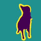
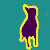
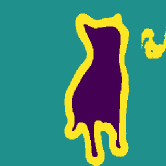
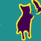
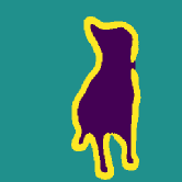
	AttUNet
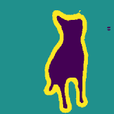
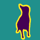
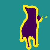
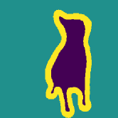
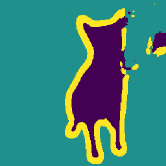
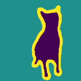
	NestUNet

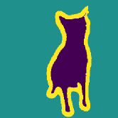
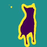
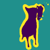
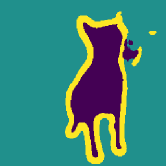
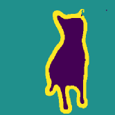
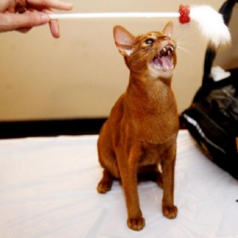
(a) Image

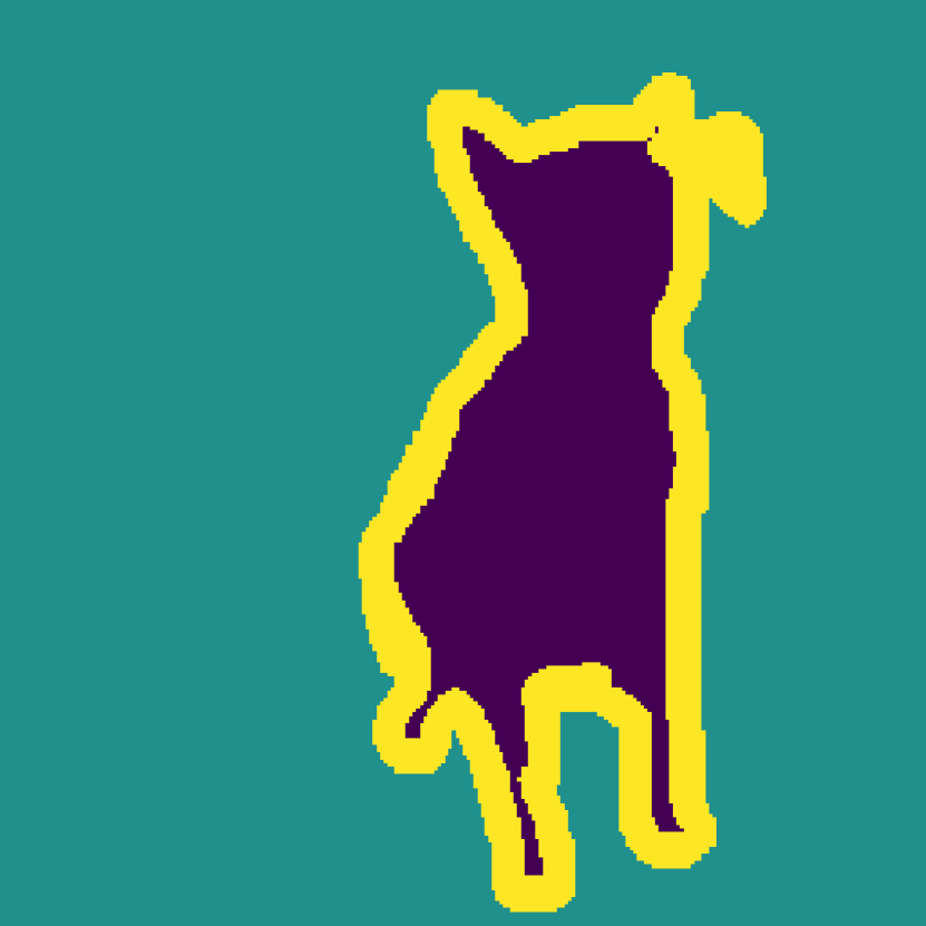
(b) Label

Figure 5: Visualization of segmentation performance on OxfordPetIII dataset trained by different model architectures including UNet, AttUNet, and NestUNet.

5.2.3 Training performance.

Owing to the demand of taking full advantage of big data which is not only a large scaled number of samples but also high pixel resolution[31], a method that is low cost in both computation and memory usage is essential. To investigate the performance of different methods, we use three metrics including the average training time (seconds/epoch), the average memory acquisition, and the average GPU utilization. We calculate these metrics in each epoch and then take the average value once the training is done.

Fig. 6 suggests that our proposed method (pink circle), which includes the LA and PAT can adapt to a wide range of hardware specifications. While the proposed method acquires roughly 15GB, recent methods (i.e. BLV, LDAM) acquire nearly 17GB and 20GB in the OxfordPetIII and NyU datasets, respectively. In the CityScapes dataset, the proposed method is one of the three lowest GPU-utilized methods, along with the vanilla cross-entropy loss function, which also refers to the lowest time-consumed method.

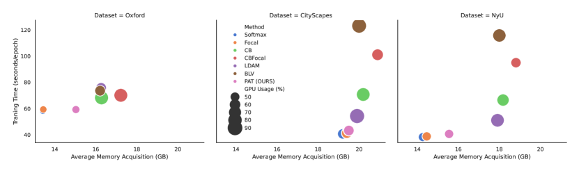
Figure 6: Performance comparison between baselines and our proposed method in three different scenarios containing OxfordPetIII, CityScapes, and NyU. Performance metrics include Training Time (seconds/epoch), Average Memory Acquisition shown in Gigabyte (GB) units, and the GPU Utilization proportion (%). Note that all experiments are conducted using SegNet[2] model architecture.

5.3 Limitations

Segmentation datasets often exhibit two main types of imbalance including class imbalance (some classes appear more common than others) and size imbalance (some objects account for more proportion than others inside one mask sample)[28]. Through deep empirical analyses, our proposed method can tackle the issues of detecting long-tailed rare objects as well as keeping good performance on well-classified and large proportion categories. However, several key areas still require improvement.

First, although PAT only accounts for a smaller amount of memory, the amount of memory acquired by PAT is still much larger than the Focal and CE. The GPU utilization needed for PAT is not an exception, which is also much higher than Focal and CE, which refers to Fig. 6. This high computation and memory is owing to the large number of calculations needed for the exponential function, though it is a smooth and differentiated function along with its ability to put a high scalarization on low confidence classes.

Second, sharing a common challenge with other semantic segmentation techniques, our proposed method (PAT) is notably susceptible to domain shift. This means that the model’s output predictions (logits) differ significantly across different data domains, making it difficult to determine the optimal scaling loss coefficient. Consequently, applying the model trained on one domain (source) to another domain (target) can result in substantial performance degradation. Future work could address this issue by incorporating domain generalization techniques, such as those described in [23, 32, 14], into the semantic segmentation framework.

6 Conclusion

We introduce the Pixel-wise Adaptive Training (PAT) technique for long-tailed segmentation. Leveraging class-wise gradient magnitude homogenization and pixel-wise class-specific loss adaptation, our approach alleviates gradient divergence due to label mask size imbalances, and the detrimental effects of rare classes and frequent class forgetting issues. Empirically, on the NyU dataset, PAT achieves a $2.85\%$ increase in mIoU compared to the baseline. Similar improvements are observed in the CityScapes dataset ($2.2\%$ increase) and the OxfordPetIII dataset ($0.09\%$ increase). Furthermore, visualizations reveal that PAT-trained models effectively segment long-tailed rare objects without forgetting well-classified ones.

References

- [1] Alexandridis, K.P., Deng, J., Nguyen, A., Luo, S.: Long-tailed instance segmentation using gumbel optimized loss. In: ECCV. pp. 353–369 (2022)
- [2] Badrinarayanan, V., Kendall, A., Cipolla, R.: Segnet: A deep convolutional encoder-decoder architecture for image segmentation. IEEE TPAMI (2017)
- [3] Bai, J., Liu, Z., Wang, H., Hao, J., FENG, Y., Chu, H., Hu, H.: On the effectiveness of out-of-distribution data in self-supervised long-tail learning. In: The Eleventh International Conference on Learning Representations (2023)
- [4] Cao, K., Wei, C., Gaidon, A., Arechiga, N., Ma, T.: Learning imbalanced datasets with label-distribution-aware margin loss. In: NeurIPS (2019)
- [5] Cordts, M., Omran, M., Ramos, S., Rehfeld, T., Enzweiler, M., Benenson, R., Franke, U., Roth, S., Schiele, B.: The cityscapes dataset for semantic urban scene understanding. In: CVPR (2016)
- [6] Cui, Y., Jia, M., Lin, T.Y., Song, Y., Belongie, S.: Class-balanced loss based on effective number of samples. In: CVPR. pp. 9260–9269 (2019)
- [7] Dong, B., Zhou, P., Yan, S., Zuo, W.: LPT: Long-tailed prompt tuning for image classification. In: The Eleventh International Conference on Learning Representations (2023)
- [8] Gupta, A., Dollar, P., Girshick, R.: Lvis: A dataset for large vocabulary instance segmentation. In: CVPR (June 2019)
- [9] He, Y.Y., Zhang, P., Wei, X.S., Zhang, X., Sun, J.: Relieving long-tailed instance segmentation via pairwise class balance. In: CVPR. pp. 6990–6999 (2022)
- [10] Javaloy, A., Valera, I.: Rotograd: Gradient homogenization in multitask learning. In: ICLR (2022)
- [11] Li, R., Li, S., He, C., Zhang, Y., Jia, X., Zhang, L.: Class-balanced pixel-level self-labeling for domain adaptive semantic segmentation. In: CVPR. pp. 11593–11603 (2022)
- [12] Li, Y., Wang, T., Kang, B., Tang, S., Wang, C., Li, J., Feng, J.: Overcoming classifier imbalance for long-tail object detection with balanced group softmax. In: CVPR. pp. 10991–11000 (2020)
- [13] Lin, T.Y., Goyal, P., Girshick, R., He, K., Dollár, P.: Focal loss for dense object detection. In: ICCV. pp. 2999–3007 (2017)
- [14] Meng, R., Li, X., Chen, W., Yang, S., Song, J., Wang, X., Zhang, L., Song, M., Xie, D., Pu, S.: Attention diversification for domain generalization. In: Computer Vision – ECCV 2022 (2022)
- [15] Murray, R., Swenson, B., Kar, S.: Revisiting normalized gradient descent: Fast evasion of saddle points. IEEE Transactions on Automatic Control (2019)
- [16] Nathan Silberman, Derek Hoiem, P.K., Fergus, R.: Indoor segmentation and support inference from rgbd images. In: ECCV (2012)
- [17] Oktay, O., Schlemper, J., Folgoc, L.L., Lee, M., Heinrich, M., Misawa, K., Mori, K., McDonagh, S., Hammerla, N.Y., Kainz, B., Glocker, B., Rueckert, D.: Attention u-net: Learning where to look for the pancreas. arXiv (2018)
- [18] Pan, T.Y., Zhang, C., Li, Y., Hu, H., Xuan, D., Changpinyo, S., Gong, B., Chao, W.L.: On model calibration for long-tailed object detection and instance segmentation. In: NeurIPS (2021)
- [19] Parkhi, O.M., Vedaldi, A., Zisserman, A., Jawahar, C.V.: Cats and dogs. In: CVPR (2012)
- [20] Perrett, T., Sinha, S., Burghardt, T., Mirmehdi, M., Damen, D.: Use your head: Improving long-tail video recognition. In: 2023 IEEE/CVF Conference on Computer Vision and Pattern Recognition (CVPR) (2023)
- [21] Ren, J., Yu, C., sheng, s., Ma, X., Zhao, H., Yi, S., Li, h.: Balanced meta-softmax for long-tailed visual recognition. In: NeurIPS. pp. 4175–4186 (2020)
- [22] Ronneberger, O., Fischer, P., Brox, T.: U-net: Convolutional networks for biomedical image segmentation. In: Medical Image Computing and Computer-Assisted Intervention – MICCAI 2015 (2015)
- [23] Shi, Y., Seely, J., Torr, P., N, S., Hannun, A., Usunier, N., Synnaeve, G.: Gradient matching for domain generalization. In: ICLR (2022)
- [24] Wang, J., Zhang, W., Zang, Y., Cao, Y., Pang, J., Gong, T., Chen, K., Liu, Z., Loy, C.C., Lin, D.: Seesaw loss for long-tailed instance segmentation. In: CVPR (2021)
- [25] Wang, J., Lan, C., Liu, C., Ouyang, Y., Qin, T.: Generalizing to unseen domains: A survey on domain generalization. In: Proceedings of the Thirtieth International Joint Conference on Artificial Intelligence, IJCAI-21 (2021)
- [26] Wang, Y., Fei, J., Wang, H., Li, W., Bao, T., Wu, L., Zhao, R., Shen, Y.: Balancing logit variation for long-tailed semantic segmentation. In: CVPR. pp. 19561–19573 (2023)
- [27] Wang, Y., Fei, J., Wang, H., Li, W., Bao, T., Wu, L., Zhao, R., Shen, Y.: Balancing logit variation for long-tailed semantic segmentation. In: CVPR (2023)
- [28] Wang, Z., Berman, M., Rannen-Triki, A., Torr, P., Tuia, D., Tuytelaars, T., Gool, L.V., Yu, J., Blaschko, M.B.: Revisiting evaluation metrics for semantic segmentation: Optimization and evaluation of fine-grained intersection over union. In: Thirty-seventh Conference on Neural Information Processing Systems Datasets and Benchmarks Track (2023)
- [29] Zang, Y., Huang, C., Change Loy, C.: Fasa: Feature augmentation and sampling adaptation for long-tailed instance segmentation. In: ICCV (2021)
- [30] Zhang, C., Pan, T.Y., Chen, T., Zhong, J., Fu, W., Chao, W.L.: Learning with free object segments for long-tailed instance segmentation. In: ECCV. pp. 655–672 (2022)
- [31] Zhang, Y., Kang, B., Hooi, B., Yan, S., Feng, J.: Deep long-tailed learning: A survey. IEEE TPAMI (2023)
- [32] Zhou, K., Yang, Y., Hospedales, T., Xiang, T.: Learning to generate novel domains for domain generalization. In: Computer Vision – ECCV 2020 (2020)
- [33] Zhou, Z., Rahman Siddiquee, M.M., Tajbakhsh, N., Liang, J.: Unet++: A nested u-net architecture for medical image segmentation. In: Medical Image Computing and Computer-Assisted Intervention – MICCAI 2018 (2018)