Logic-dependent emergence of multistability, hysteresis, and biphasic dynamics in a “minimal” positive feedback network with an autoloop
Abstract
Cellular decision-making (CDM) is a dynamic phenomenon crucial for development and diseases. CDM is often, if not invariably, controlled by regulatory networks defining interactions between genes and transcription factor proteins. Traditional studies have focussed on molecular switches such as positive feedback circuits that upon multimerization exhibit at most bistability. However, higher-order dynamics such as tristability is also prominent in many biological processes. It is thus imperative to identify a ”minimal” circuit that can alone explain mono, bi, and tristable dynamics. In this work, we consider a two-component positive feedback network with an autoloop and explore these regimes of stability for different degrees of multimerization and the choice of Boolean logic functions. We report that this network can exhibit numerous dynamical scenarios such as bi-and tristability, hysteresis, and biphasic kinetics, explaining the possibilities of abrupt cell state transitions and the without a step-like switch. Specifically, while with monomeric regulation and competitive OR logic, the circuit exhibits mono-and bistability and biphasic dynamics, with non-competitive AND and logics only monostability can be achieved. To obtain bistability in the latter cases, we show that the autoloop must have (at least) dimeric regulation. In pursuit of higher-order stability, we show that tristability occurs with higher degrees of multimerization and with non-competitive logic only. Our results, backed by rigorous analytical calculations and numerical examples, thus explain the association between multistability, multimerization, and logic in this ”minimal” circuit. Since this circuit underlies various biological processes, including epithelial-mesenchymal transition which often drives carcinoma metastasis, these results can thus offer crucial inputs to control cell state transition by manipulating dimerization and the logic of regulation in cells.
Keywords: Cell fate decision; Multistability; Minimal genetic circuit; Positive feedback loop; Biphasic dynamics; Boolean logic.
1 Introduction
Cellular decision-making is a cell non-autonomous process where at each cell-lineage branch point, a cell drives into one of the alternative distinct cell types [1]. Investigating dynamical principles of regulatory networks that govern cellular decision-making is essential to understanding and controlling stepwise lineage decisions of cells [2, 3, 4]. A key aspect of this decision-making process is the ability of cells to manifest multiple stable states or phenotypes in response to varying internal and external cues without altering their genetic makeup [5, 1]. This phenomenon, known as multi-stability, is pivotal to cellular differentiation [5, 6], reprogramming [2, 1], and its manifestation through epithelial-mesenchymal plasticity [7], a cellular program enabling bidirectional transition among epithelial, mesenchymal, and one or more hybrid epithelial-mesenchymal cells, enables intra-tumor heterogeneity [8, 9], induces cancer progression and metastasis of carcinomas [10, 11]. Since cellular decision-making is largely controlled by regulatory networks defining “molecular switches” [12, 13], unraveling the dynamical behaviors and logic of multi-stable switches has profound implications in synthetic biology and regenerative medicine.
A necessary condition for nonlinear control systems and networks to exhibit multistability is the presence of positive feedback loops [14, 15, 16, 17, 13]. Interestingly, this requirement also extends to biological systems where a commonly observed network structure underlying multistability is the toggle switch [18], comprising mutual inhibition of two opposite fate-determining transcription factors thus forming a positive feedback loop. This mutual repression enables cells to adopt different states, driving an ’either-or’ binary choice between alternative cell fates from a common progenitor [2]. However, it is rational to posit that cellular decision-making doesn’t rely solely on binary outcomes. The intricate structure of gene regulatory networks enables them to exhibit multiple alternative stable states. Examples of, for instance, bi-and tristable solutions are found across biological contexts including development [19], differentiation [20, 21, 22, 23], epigenetic processes [24], and metastasis of carcinomas [25, 26, 27]. Often, a two-component system operates at the core of the underlying bistable decision-making circuits [2, 28, 29]. It is imperative to identify the ”minimal” (in terms of the number of variables and the regulatory interactions) two-component genetic circuits capable of demonstrating bistability. Two such networks are (i) circuits featuring multimeric regulation and lacking autoloop, and (ii) circuits employing monomeric regulators along with a singular monomeric autoloop [30, 12]. Jules et al., [31] and Zhang et al., [32] analytically proved that such systems can exhibit at most bistability. This begs a question: are low-dimensional networks such as two-component circuits capable of only bistable behavior or higher-order stability such as tristability (three states) can also be possible in these circuits? It may be noted that compared to bistable dynamics, networks exhibiting tristable dynamics are not much studied due to the complexity of analytical calculations as well as numerical simulations.
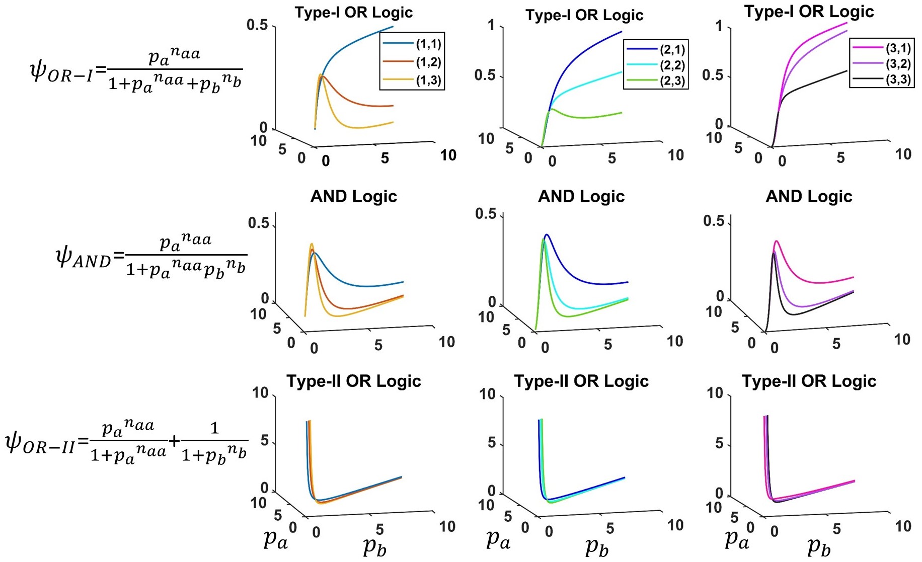
Recent theoretical and experimental studies found that miR200-ZEB positive feedback circuit with one multimeric autoloop, which underlies epithelial-mesenchymal transition, exhibits tristability [27, 26, 25, 33]. It allows reversible transition among epithelial, mesenchymal, and hybrid epithelial-mesenchymal cells and is a crucial driver of invasion and metastasis of carcinomas [34]. However, these studies are purely based on a numerical approach and lack mathematical rigor. Also, they don’t explore any association of multimerization with tristability. Motivated by this, we asked a general question: what can be the minimal ”multimeric” requirements for a two-component feedback network with one autoloop (Fig. 1a) to exhibit mono-and bistability and under what conditions can it exhibit tristability? Further, node is co-regulated by node and node itself through autoloop. When a gene is regulated by more than one transcription factor, the combinatorial rule (Boolean logic) must also be considered. We considered three types of regulatory logic: (a) Competitive OR logic, (b) non-competitive AND logic, and (c) non-competitive OR logic, and explored their effect on the order of stability. For simplicity, throughout the text, we denote these three logics as Type-I OR, AND, and Type-II , respectively.
In this work, we thus analyze the dynamics of such a generic, minimal network (depicted in Fig. 1a) by systematically finding the analytical conditions for mon, bi, and tristable dynamical regimes. We model the network using a system of coupled ordinary differential equations for which each stable equilibrium solution corresponds to a possible stable state (or phenotype or attractor). We explore how these solutions are affected by the degree of multimerization as well as the type of regulatory logic. We integrated the autoloop with the core positive feedback network using three regulatory logics: AND gate, Type-I OR gate, and Type-II gate, each having a different mathematical formalism and qualitative behavior (Fig. 1b). Starting with monomeric regulation, we systematically tested higher degrees of multimerization in each model. We report that multistability in this network is logic-dependent. In monomeric regulation with monomeric autoloop, while type-I OR logic exhibits at most bistability, AND and type-II logic can exhibit only monostability. To obtain bistability with AND and Type-II logics, we show that a dimeric autoloop is required. Upon testing different combinations of multimerization, we show that tristability can occur in higher degrees of multimerization, though bistability is persistently prevalent irrespective of the logic of regulation. Our results thus comprehensively provide an association between multistability, multimerization, and logic in this circuit. Since this circuit underlies various biological processes including EMT in cancers and the multistability can be mapped to phenotypic heterogeneity, these results can thus offer crucial inputs to control phenotypic heterogeneity by manipulating dimerization and synthetically (re)engineering the logic of regulation in cells.
![[Uncaptioned image]](/html/2404.05379/assets/x1.png)
2 Organization of the paper
This paper contains three main sections based on the three different types of Boolean logic used to model the co-regulation of gene by two transcription factors. In section 3, this co-regulation is modeled using competitive OR logic. In section 4, the non-competitive AND logic is employed. In section 5, a non-competitive logic is considered to model the co-regulation. For brevity, throughout the text, competitive OR logic, non-competitive AND logic, and non-competitive OR logic are referred to as Type-I OR logic, AND logic, and Type-II logic, respectively. In each section, we explore the minimal multimerization conditions (manifested through Hill coefficient values) for the occurrence of mono, bi-and multistability. We have applied the nullcline approach to show the existence of steady states. For each model, we analyze the associated characteristic equations and obtain the conditions for the stability of the steady states and the existence of saddle-node bifurcations. Numerical simulations are then performed to illustrate the results. Through bifurcations, we also present possible ways of state transitions such as step-like abrupt state transition (a manifestation of saddle-node bifurcation) and biphasic (manifested through sigmoidal curves). In Section 6, we discuss the impact of basal production rate (leakage) on each model’s dynamics. Finally, section 7 presents a detailed discussion and concluding remarks based on our findings.
3 Mathematical Model [Type-I OR Logic]
The model under investigation in this paper is depicted in Fig. 1. The complete nonlinear mathematical model uses four state variables for the concentrations of mRNAs and transcription factor proteins (TF). The concentration of mRNA produced by genes and is denoted by and respectively, while the corresponding TF protein concentrations are denoted by and The inhibition of gene and by TF and , respectively, is modelled by the Hill function. Also, the activation of gene by its own TF, , is modeled by the Hill function with a different Hill coefficient, . The co-regulation of gene by TF and also by its own TF is modeled using competitive OR logic [35]. The transcription of genes and into mRNA and is modeled using the non-linear Hill function while the translation of these mRNA’s into TF proteins and is modeled using linear mass-action kinetics.
Using the above formalism, the following system of coupled nonlinear ordinary differential equations describe the dynamics of the network in Fig. 1.
| (1) | ||||
with where are the maximum transcription rates, are the mRNA degradation rates, are the translation rates, and are the protein degradation rates for genes . and represent the basal production rates (in the absence of activation and inhibition) of genes and respectively. The threshold parameters denote the thresholds of and to induce a significant response of and . The integer parameters and are Hill coefficients that determine the steepness of Hill curves.
3.1 Mathematical Analysis
This section presents the existence and stability analysis of the steady states for the model system (1). We use the Routh-Hurwitz criterion [36] to prove the local asymptotic stability of the steady states, while Sotomayor’s theorem [36] is used to derive the transversality conditions of saddle-node bifurcation.
We obtained the steady state by setting the right hand side of the model (1) to zero. From third and fourth equations of model (1), we obtained and respectively, as and Using and then putting the value of we get Finally, using the value of and in we get a polynomial in as
| (2) |
where and Here, is a positive real root of (2) which we discuss in different cases explicitly.
Case 1: When then from (1), we get a cubic polynomial in
| (3) |
where and The nature of the curve can be observe from (3) as
-
(i)
because
-
(ii)
as because
-
(iii)
The number of positive real roots of equation (3) can be seen using Descarte’s rule of sign, mentioned in below Table (1).
Coefficients Number of possible positive real roots of A B C D + - - - 1 + + - - 1 + + + - 1 + - + - 3,1 Table 1: Number of possible positive real roots of
Therefore, will have either unique or three positive real roots.
Case 2: When then from (1), we get a quartic polynomial in
| (4) |
where and
The number of positive real roots of equation (4) can be seen using Descarte’s rule of sign, mentioned in below Table (2).
| Coefficients | Number of possible positive real roots of | ||||
|---|---|---|---|---|---|
| A | B | C | D | E | |
| + | - | + | - or + | - | 3, 1 |
| + | + or - | - | + | - | 3, 1 |
| + | + or - | - | - | - | 1 |
| + | + | + | - or + | - | 1 |
Case 3: When then from (1), we get a quintic polynomial in
| (5) |
where and
The nature of curve can be observe from (3) as
-
(i)
because
-
(ii)
as because
-
(iii)
will have either unique or three or five positive real roots.
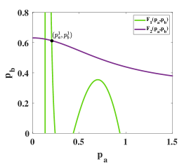
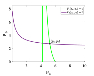
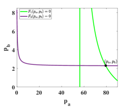
To deal with the fifth-degree polynomial with parametric coefficients is quite difficult, so we use the nullcline method to further analyze the existence of possible positive real roots. From the system (1), we have
| (6) | ||||
First to observe the nature of curve we reduce it in the form of
| () |
The following conclusion can be made from ()
-
(i)
-
(ii)
as
-
(iii)
, i.e, is a decreasing function of
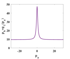
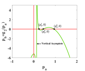
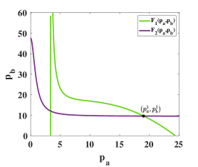
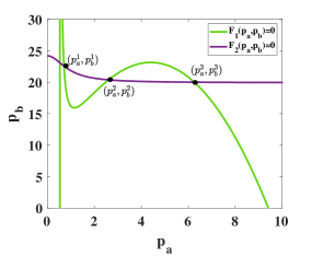
The graph of (or ) is shown in Fig. 2 (a).
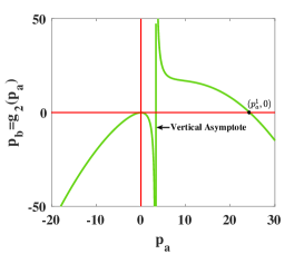
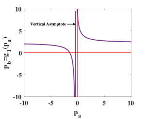
Now, to observe the nature of curve we reduce it in the form of
| () |
The following conclusion can be made from ()
-
(i)
is a rational function and it has an asymptote at .
-
(ii)
The positive intercept can be find with which implies that the positive real roots of will provide the positive intercept of
-
(iii)
The -intercept of is negative.
-
(iv)
We note that for , we have so if positive real roots of exits then it always lie on the right-hand side of asymptote.
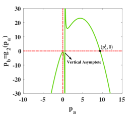
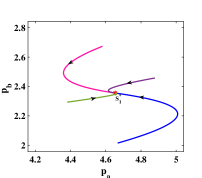
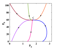
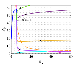
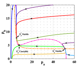
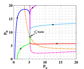
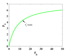
The possibility of unique positive -intercept of is shown in Fig. 2 (b) and Fig. 2 (c). With unique positive -intercept, there can be unique and three positive steady states, as shown in Fig. 3 (a) and Fig. 3 (b), respectively. In Fig. 2 (d), we have shown the three positive -intercept of , and for this case, we obtain three and unique positive steady states, as shown in Fig. 3 (c) and Fig. 3 (d), respectively. Therefore, from the above discussion, we discard the case of five positive steady states.
3.1.1 Local stability of steady state
Theorem 1.
The steady state is locally asymptotically stable if and where are provided in the proof.
3.1.2 Saddle Node Bifurcation
We derive the transversality condition for saddle-node bifurcation considering as a bifurcation parameter for system (1). Let is the threshold value of for the occurrence of saddle-node bifurcation.The system (1) has two steady states () for collide () at and then disappear when . The point of collision is represented as Define where and are defined as
Let the Jacobian matrix has a simple eigenvalue with eigenvector , and the transpose of the Jacobian matrix has an eigenvector to the eigenvalue Then the model system (1) experiences a saddle-node bifurcation at , if the following transversality conditions [36] are satisfied:
| () |
and
| () | ||||
where
3.1.3 Numerical simulation and discussion corresponding to model (1)
The purpose of this section is to provide validation for the theoretical results that were covered in Subsection 3.1. We have talked about the system’s behavior in terms of monostability and bi-stability with fictitious parameters.
Example 1.
(case 1) and other parameters are chosen as
In this range of there is unique () steady state in , three () in and unique () in such that where and The steady states are stable and () is unstable. The corresponding bifurcation diagram is shown in Fig. 4 (a).
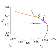
To ensure the stability of we chosen and the coefficients of characteristic equation at are calculated as and Therefore, from Theorem 1, we conclude that is locally asymptotically stable. We draw the phase portrait for the considered parameters, shown in Fig. 4 (b). We can see that all trajectories starting from any initial points are converging to
Further, we chosen and the coefficients of characteristic equation at are calculated as and The coefficients of characteristic equation at are calculated as and The coefficients of characteristic equation at are calculated as and Therefore, from Theorem 1, we conclude that is locally asymptotically stable and is unstable. We draw the phase portrait for the considered parameters, shown in Fig. 4 (c). We can see that all trajectories are converging to and nearby trajectories of are moving away from This shows the bistable behaviour of the system.
We chosen
the coefficients of characteristic equation at
are calculated as and Therefore, from Theorem 1, we conclude that is locally asymptotically stable. We draw the phase portrait for the chosen parameters, shown in Fig. 4 (d). We can see that all trajectories starting from any initial points are converging to
For this case, again we choose the parameters as For this set of parameters, we obtain a unique stable steady state as discussed in Case 1. The corresponding bifurcation plot is shown in Fig. 4 (e). To ensure the stability of we choose from the range of The coefficients of characteristic equation at are calculated as and Therefore, from Theorem 1, we conclude that is locally asymptotically stable. We draw the phase portrait for the considered , shown in Fig. 4 (f). We can see that all trajectories starting from any initial points are converging to
In this example, we also discuss the case of saddle-node bifurcation. We have seen that the system (1) has two steady states in such that as the value of decreases, the two steady states collide at and denoted as The Jacobian matrix has a simple eigenvalue and
, are the eigenvectors of and respectively. Both the tranversality conditions and
are satisfied. Hence, the system (1) experiences saddle-node bifurcation at Also, the system (1) has two steady states in such that as the value of increases, the two steady states collide at and denoted as The Jacobian matrix has a simple eigenvalue and , are the eigenvectors of and respectively. Both the tranversality conditions and are satisfied. Hence, the system (1) experiences saddle-node bifurcation at
Example 2.
(case 2), and the other parameters are chosen as:
In this range of there is unique () steady state in , three () in and unique () in such that where and The steady states are stable and () is unstable. The corresponding bifurcation diagram is shown in Fig. 5 (a).
To ensure the stability of we chosen and the coefficients of characteristic equation at are calculated as and Therefore, from Theorem 1, we conclude that is locally asymptotically stable. We draw the phase portrait for the considered parameters, shown in Fig. 5 (b). We can see that all trajectories starting from any initial points are converging to
Further, we chosen and the coefficients of characteristic equation at are calculated as and The coefficients of characteristic equation at are calculated as and The coefficients of characteristic equation at are calculated as and Therefore, from Theorem 1, we conclude that is locally asymptotically stable and is unstable. We draw the phase portrait for the considered parameters, shown in Fig. 5 (c). We can see that all trajectories are converging to and nearby trajectories of are moving away from This shows the bistable behavior of the system.
We chosen
the coefficients of characteristic equation at
are calculated as and Therefore, from Theorem 1, we conclude that is locally asymptotically stable. We draw the phase portrait for the chosen parameters, shown in Fig. 5 (d). We can see that all trajectories starting from any initial points are converging to
In this example, we also discuss the case of saddle-node bifurcation. We have seen that the system (1) has two steady states in such that as the value of decreases, the two steady states collide at and denoted as The Jacobian matrix has a simple eigenvalue and
, are the eigenvectors of and respectively. Both the tranversality conditions and
are satisfied. Hence, the system (1) experiences saddle-node bifurcation at Also, the system (1) has two steady states in such that as the value of increases, the two steady states collide at and denoted as The Jacobian matrix has a simple eigenvalue and , are the eigenvectors of and respectively. Both the tranversality conditions and are satisfied. Hence, the system (1) experiences saddle-node bifurcation at
The system (1) exhibits a hysteresis effect in where multiple steady states coexist, as
shown in Fig. 4 (a) and Fig 5 (a). The two outer steady states are stable, while the interior steady state (red) is
unstable.
For this case, again we choose and other parameters are the same as above. We obtained a unique steady state that is stable throughout the range of considered The corresponding bifurcation diagram is shown in Fig. 5 (e). The phase trajectory for is shown in Fig. 5 (f). All trajectories are converging to
Example 3.
(case 3), and the other parameters are chosen as: In this range of there is unique () steady state in , three () in and unique in such that where and The steady states are stable and () is unstable. The corresponding bifurcation diagram is shown in Fig. 6 (a). All other descriptions are the same as those discussed in Example 2.
Example 4.
(case 4), and the other parameters are chosen as:
In this range of there is unique () steady state in , three () in and unique in such that where and The steady states are stable and () is unstable. The corresponding bifurcation diagram is shown in Fig. 6 (b). All other descriptions are the same as discussed in Example 2.
Now, we discuss some other cases in which we observe the monostable and bistable behavior of the system. Instead of showing bifurcation diagrams, here we show the phase portraits with null clines.
If , and the other parameters are chosen as:
For this parameter, we obtained three steady states and
which are nodal sink (stable), saddle point (unstable) and nodal sink, respectively. The corresponding phase portrait diagram is shown in Fig. 7 (a). Further, for this case, we choose we obtained unique steady state which is locally asymptotically stable (nodal sink), shown in Fig. 7 (b).
If , and the other parameters are chosen as same as the case of For this parameter, we obtained three steady states and which are nodal sink (stable), saddle point (unstable) and nodal sink, respectively. Fig. 8 (a) shows the corresponding phase portrait diagram. Further, for this case, we choose we obtained unique steady state which is locally asymptotically stable (nodal sink), shown in Fig. 8 (b).
3.2 Conclusion and biological interpretation for this section
In this section, we assume that the two genes and compete for binding to the promoter regions and any of the binding events can elicit gene expression. This type of biological regulation is modeled using a competitive OR logic function. Our results show that with any combination and degree of multimerization (Hill coefficient values), the network will exhibit at most bistability. We also found that cell state transition can occur through two mechanisms: (i) hysteresis; in which the cell remembers the past state and abruptly switches back and forth to another state as the input signal crosses a certain threshold (Fig.’s 4a, 5a, 6). (ii) biphasic transition; in which we observe that cells can transit to the next state without a step-like switch (4c, 5e). In this situation, there is no bifurcating attractor and hence no cells are ”forced” to transition, instead, gene expression changes in a smooth continuous way.
4 Mathematical Model [AND Logic]
In this section, we model the co-regulation of node using non-competitive AND logic [35]. With this formalism, the model system takes the following form.
| (8) | ||||
with The parameter description is same as Section 3.
4.1 Mathematical Analysis
This subsection again presents the existence and stability analysis of the steady states for the model system (8). We use the Routh-Hurwitz criterion to prove the local asymptotic stability of the steady states, while Sotomayor’s theorem is used to derive the transversality conditions of saddle-node bifurcation.
We obtained the steady state by setting the right hand side of the model (1) to zero. From third and fourth equations of model (1), we obtained and respectively, as and Using and then putting the value of we get Finally, using the value of and in we get a polynomial in as
| (9) |
where and Here, is a positive real root of (9) which we discuss in different cases explicitly.
Case 1: When then from (9), we get a cubic polynomial in
| (10) |
where and The nature of the curve can be observe from (10) as
-
(i)
because
-
(ii)
as because
-
(iii)
The number of positive real roots of equation (10) can be seen using Descarte’s rule of sign, mentioned in below Table (3).
Coefficients Number of possible positive real roots of A B C D - - - + 1 - + - + 3,1 - + + + 1 - - + + 1 Table 3: Number of possible positive real roots of
Therefore, will have either unique or three positive real roots. Now, to discard the existence of three positive real roots, we use the nullcline method. From the system (8), we have
| (11) | ||||
First to observe the nature of curve we reduce it in the form of
| () |
The following conclusion can be made from ()
-
(i)
-
(ii)
as
-
(iii)
, i.e, is a decreasing function of
The graph of (or ) is shown in Fig. 9.
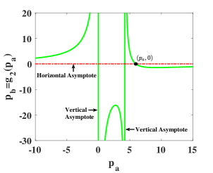
Now, to observe the nature of curve we reduce it in the form of
| () |
Equivalently
| () |
Also, we find
| () |
Equivalently
| () |
The following conclusion can be made from ()
-
(i)
is a rational function, and it has two vertical asymptotes at and and (i.e., -axis) is a horizontal asymptote.
-
(ii)
We note that for , we have so if positive real roots of exits then it always lie on the right-hand side of vertical asymptote .
-
(iii)
The intercept can be find with which implies that The sign of will provide the unique intercept of Now, we will discuss three cases to understand the nature of curve
-
(a)
When and then there will no positive intercept; also and which implies that is strictly decreasing. The corresponding diagram is shown in Fig. 10 (a).
- (b)
-
(a)
All possibilities of the existence of a steady state are shown in Fig. 10 (b) and Fig. 10 (d) corresponding to 10 (a) and Fig. 10 (c), respectively. Therefore, from the above discussion, we discard the existence of three positive steady states.
![[Uncaptioned image]](/html/2404.05379/assets/x29.png)
![[Uncaptioned image]](/html/2404.05379/assets/x30.png)
Case 2: When then from (8), we get a quartic polynomial in
| (12) |
where and
The number of positive real roots of equation (12) can be seen using Descarte’s rule of sign (mentioned in below Table (2)); therefore, will have either unique or three positive real roots.
4.1.1 Local stability of steady state
Theorem 2.
The steady state is locally asymptotically stable if and where are provided in the proof.
4.1.2 Saddle Node Bifurcation
We find the transversality condition the same as discussed in Subsection 3.1.2. Define where are defined as
and and expression is same as Subsection 3.1.2. Then the model system (8) experiences a saddle-node bifurcation at , if the following transversality conditions [36] are satisfied:
| () |
and
| () |
where and
4.1.3 Numerical simulation and discussion corresponding to model system (8)
The purpose of this section is to provide validation for the theoretical results that were covered in Subsection 4.1. We have talked about the system’s behavior in terms of monostability and bi-stability with fictitious parameters.
Example 5.
(case 1) and the other parameters are chosen as For this set of parameters, we obtain a unique stable steady state as discussed in Case 1(and). The corresponding bifurcation plot is shown in Fig. 11 (a). To ensure the stability of we choose from the range of The coefficients of characteristic equation at are calculated as and Therefore, from Theorem 2, we conclude that is locally asymptotically stable. We draw the phase portrait for the considered , shown in Fig. 11 (b). We can see that all trajectories starting from any initial points are converging to
Example 6.
(case 2), and the other parameters are chosen as:
In this range of there is unique () steady state in , three () in and unique () in such that where and The steady states are stable and () is unstable. The corresponding bifurcation diagram is shown in Fig. 12 (a).
To ensure the stability of we chosen and the coefficients of characteristic equation at are calculated as and Therefore, from Theorem 2, we conclude that is locally asymptotically stable. We draw the phase portrait for the considered parameters, shown in Fig. 12 (b). We can see that all trajectories starting from any initial points are converging to
Further, we chosen and the coefficients of characteristic equation at are calculated as and The coefficients of characteristic equation at are calculated as and The coefficients of characteristic equation at are calculated as and Therefore, from Theorem 2, we conclude that is locally asymptotically stable and is unstable. We draw the phase portrait for the considered parameters, shown in Fig. 12 (c). We can see that all trajectories are converging to and nearby trajectories of are moving away from This shows the bistable behaviour of the system.
We chosen
the coefficients of characteristic equation at are calculated as and Therefore, from Theorem 2, we conclude that is locally asymptotically stable. We draw the phase portrait for the chosen parameters, shown in Fig. 12 (d). We can see that all trajectories starting from any initial points are converging to
In this example, we also discuss the case of saddle-node bifurcation. We have seen that the system (8) has two steady states in such that as the value of decreases, the two steady states collide at and denoted as The Jacobian matrix has a simple eigenvalue and
, are the eigenvectors of and respectively. Both the tranversality conditions and
are satisfied. Hence, the system (1) experiences saddle-node bifurcation at Also, the system (8) has two steady states in such that as the value of increases, the two steady states collide at and denoted as The Jacobian matrix has a simple eigenvalue and , are the eigenvectors of and respectively. Both the tranversality conditions and are satisfied. Hence, the system (8) experiences saddle-node bifurcation at
The system (8) exhibits a hysteresis effect in where multiple steady states coexist, as
shown in Fig 12 (a). The two outer steady states are stable, while the interior steady state (red) is
unstable.
Again, in this case, the parameters are chosen as For this set of parameters, we obtain a unique stable steady state as discussed in Case 2 (AND). The corresponding bifurcation plot is shown in Fig. 12 (e). To ensure the stability of we choose from the range of The coefficients of characteristic equation at are calculated as and Therefore, from Theorem 2, we conclude that is locally asymptotically stable. We draw the phase portrait for the considered , shown in Fig. 12 (f). We can see that all trajectories starting from any initial points are converging to
![[Uncaptioned image]](/html/2404.05379/assets/x35.png)
![[Uncaptioned image]](/html/2404.05379/assets/x36.png)
![[Uncaptioned image]](/html/2404.05379/assets/x37.png)
4.2 Conclusion and biological interpretation for this section
In this section, we assume that the two genes and don’t compete for binding to the promoter regions. However, only both binding events can elicit gene expression. This type of biological regulation is modeled using a non-competitive AND logic function. Our results show that, unlike competitive binding with OR logic, AND logic can’t produce bistability with monomeric regulations (Hill coefficients of degree 1). We show that bistability requires dimeric (Hill coefficients of degree 2) autoloop. We also show that only through ”forced” cell state transition (hysteresis) and not the smooth state swap (biphasic transition) is possible with this logic function for all combinations of dimerizations.
5 Mathematical Model [Type-II Logic]
In this section, we model the co-regulation of node using non-competitive OR logic [35]. With this formalism, the model system takes the following form.
| (14) | ||||
with Parameter description is same as Section 3.
5.1 Mathematical Analysis
We get the steady state by setting the right hand side of the model (14) to zero. From third and fourth equations of model (14), we obtained and respectively, as and Using and then putting the value of we get Finally, using the value of and in we get a polynomial in as
| (15) | ||||
where and Here, is a positive real root of (15) which we discuss in different cases explicitly.
Case 1: When then from (15), we get a cubic polynomial in
| (16) |
where and The nature of the curve can be observe from (16) as
-
(i)
because
-
(ii)
as because
- (iii)
Therefore, will have either unique or three positive real roots. Now, to discard the existence of three positive real roots, we use the nullcline method. From the system (14), we have
| (17) | ||||
First to observe the nature of curve we reduce it in the form of
| () |
The following conclusion can be made from ()
-
(i)
-
(ii)
as
-
(iii)
, i.e, is a decreasing function of
The graph of (or ) is shown in Fig. 9.
Now, to observe the nature of curve we reduce it in the form of
| () |
The following conclusion can be made from ()
-
(i)
The intercept of are and . We note that and which means we have one positive and one negative intercept. Also intercept is negative, i.e.
-
(ii)
is a rational function, and it has two vertical asymptotes at
and
.
We note that and which means we have one positive and one negative vertical asymptotes. Moreover, is a horizontal asymptote.
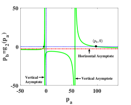
We note that For we have and for we have Also, which implies that is strictly decreasing. The corresponding diagram is shown in Fig. 13 (a). Therefore, from the above discussion regarding the nature of and , we conclude that there exists a unique steady state, shown in Fig. 13 (b), and we discard the case of three positive steady states.
Case 2: When then from (15), we get a quartic polynomial in
| (18) |
where and
The number of positive real roots of equation (18) can be seen using Descarte’s rule of sign (mentioned in Table (2)); therefore, will have either unique or three positive real roots.
Case 3: When then from (15), we get a ninth degree polynomial in
| (19) |
where
and
The number of positive real roots of equation (19) can be obtained using Descarte’s rule of sign. Due to complexity of polynomial, we discuss the existence of steady states via numerical simulation.
5.1.1 Local stability of steady state
Theorem 3.
The steady state is locally asymptotically stable if and where are provided in the proof.
5.1.2 Saddle Node Bifurcation
We find the transversality condition the same as discussed in Subsection 3.1.2. Define where are defined as
and the expression of and are same as Subsection 3.1.2. Then the model system (14) experiences a saddle-node bifurcation at , if the following transversality conditions [36] are satisfied:
| () |
and
| () |
where and
5.1.3 Numerical simulation and discussion corresponding to model system (14)
The purpose of this section is to provide validation for the theoretical results that were covered in Subsection 5.1. We have talked about the system’s behavior in terms of monostability, bistability, and tristability with fictitious parameters.
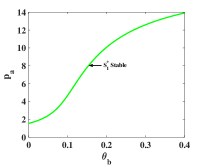
Example 7.
(case 1) and the other parameters are chosen as For this set of parameters, we obtain a unique stable steady state as discussed in Case 1. The corresponding bifurcation plot is shown in Fig. 14 (a). To ensure the stability of we choose from the range of The coefficients of characteristic equation at are calculated as and Therefore, from Theorem 3, we conclude that is locally asymptotically stable. We draw the phase portrait for the considered , shown in Fig. 14 (b). We can see that all trajectories starting from any initial points are converging to
Example 8.
(case 2), and the other parameters are chosen as:
In this range of there is unique () steady state in , three () in and unique () in such that where and The steady states are stable and () is unstable. The correspond bifurcation diagram is shown in Fig. 15 (a).
To ensure the stability of we chosen and the coefficients of characteristic equation at are calculated as and Therefore, from Theorem 3, we conclude that is locally asymptotically stable. We draw the phase portrait for the considered parameters, shown in Fig. 15 (b). We can see that all trajectories starting from any initial points are converging to
Further, we chosen and the coefficients of characteristic equation at are calculated as and The coefficients of characteristic equation at are calculated as and The coefficients of characteristic equation at are calculated as and Therefore, from Theorem 3, we conclude that is locally asymptotically stable and is unstable. We draw the phase portrait for the considered parameters, shown in Fig. 15 (c). We can see that all trajectories are converging to and nearby trajectories of are moving away from This shows the bistable behavior of the model system (14).
We chosen
the coefficients of characteristic equation at are calculated as and Therefore, from Theorem 3, we conclude that is locally asymptotically stable. We draw the phase portrait for the chosen parameters, shown in Fig. 15 (d). We can see that all trajectories starting from any initial points are converging to
In this example, we also discuss the case of saddle-node bifurcation. We have seen that the system (14) has two steady states in such that as the value of decreases, the two steady states collide at and denoted as The Jacobian matrix has a simple eigenvalue and
, are the eigenvectors of and respectively. Both the tranversality conditions and
are satisfied. Hence, the system (14) experiences saddle-node bifurcation at Also, the system (14) has two steady states in such that as the value of increases, the two steady states collide at and denoted as The Jacobian matrix has a simple eigenvalue and , are the eigenvectors of and respectively. Both the tranversality conditions and are satisfied. Hence, the system (14) experiences saddle-node bifurcation at
The system (14) exhibits a hysteresis effect in where multiple steady states coexist, as
shown in Fig 15 (a). The two outer steady states are stable, while the interior steady state (red) is unstable.
Again, in this case, the parameters are chosen as For this set of parameters, we obtain a unique stable steady state as discussed in Case 2 (OR2). The corresponding bifurcation plot is shown in Fig. 15 (e). To ensure the stability of we choose from the range of The coefficients of characteristic equation at are calculated as and Therefore, from Theorem 3, we conclude that is locally asymptotically stable. We draw the phase portrait for the considered , shown in Fig. 15 (f). We can see that all trajectories starting from any initial points are converging to
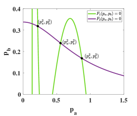
Example 9.
(case 3) and the other parameters are chosen as
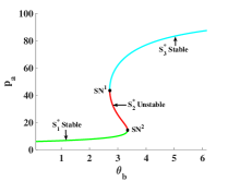
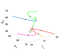
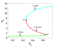
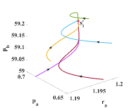
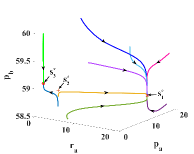
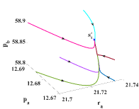
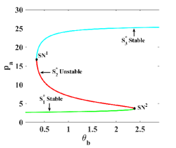
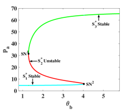
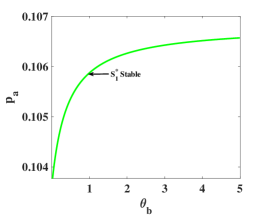
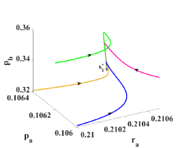
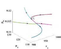
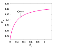
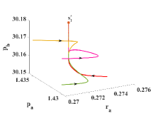
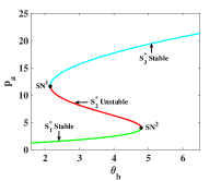
In this range of there is three () steady states in , five () in three ( in and unique () in such that where and The steady states are stable and are unstable. The corresponding bifurcation diagram is shown in Fig. 16 (a).
To ensure the tristability in we chosen and the coefficients of characteristic equation at are calculated as and
The coefficients of characteristic equation at are calculated as and
The coefficients of characteristic equation at are calculated as and
The coefficients of characteristic equation at are calculated as and
The coefficients of characteristic equation at are calculated as and
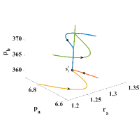
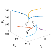
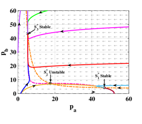
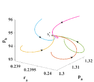
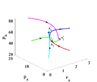
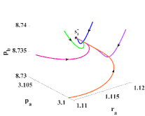
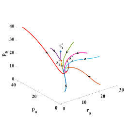
Therefore, from Theorem 3, we conclude that are locally asymptotically stable and are unstable. We draw the phase portrait for the considered parameters, shown in Fig. 16 (b). We can see that all trajectories starting from any initial points are converging to and nearby trajectories of are moving away from This shows the tristable behavior of the model system (14).
Further, to ensure the bistability in we chosen and the coefficients of characteristic equation at are calculated as and
The coefficients of characteristic equation at are calculated as and
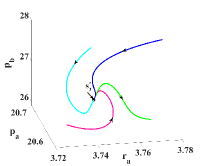
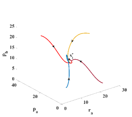
The coefficients of the characteristic equation at are calculated as and Therefore, from Theorem 3, we conclude that are locally asymptotically stable and is unstable. We draw the phase portrait for the considered parameters, shown in Fig. 16 (c). We can see that all trajectories are converging to and nearby trajectories of are moving away from This shows the bistable behavior of the model system (14).
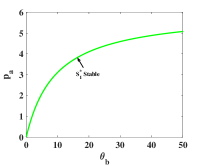
To ensure the mono-stability in we chosen and
the coefficients of characteristic equation at are calculated as and Therefore, from Theorem 3, we conclude that is locally asymptotically stable. We draw the phase portrait for the chosen parameters, shown in Fig. 16 (d). We can see that all trajectories starting from any initial points are converging to
![[Uncaptioned image]](/html/2404.05379/assets/x51.png)
![[Uncaptioned image]](/html/2404.05379/assets/x52.png)
5.2 Conclusion and biological interpretation for this section
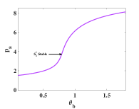
In this section, we consider a non-competitive type-II logic as an alternate to competitive OR logic. Here we assume that the two genes and don’t compete for binding and any binding events can elicit gene expression. Our results overlap with that of AND logic by showing that bistability requires dimeric (Hill coefficients of degree 2) autoloop and cell state transition can occur only through abrupt transitions (hysteresis). Nevertheless, the main result of this section is tristability, which we show is possible only in higher degrees of multimerization (e.g., ()). One manifestation of tristability is phenotypic heterogeneity (concurrent occurrence of three phenotypes) and we also observe that cell transition occurs abruptly after a certain threshold of is crossed (Fig. 16a). We thus conclude that an autoregulated two-node positive feedback circuit with non-competitive OR logic (type-II ) is the ”minimal” circuit to exhibit multistability under higher degrees of multimerization.
6 Impact of basal production rate on model dynamics
Basal production rate or leakage defines the production of mRNA in the absence of any activatory or inhibitory interacting transcription factors. For instance, the basal production of will be the rate of production of in ”normal” conditions, i.e., when the self-activation due to itself or inhibition by is absent. While modeling gene expression (transcription) processes, leakage is sometimes neglected at the cost of simplifying modeling efforts and analytical calculations. However, in all of our model systems, (1), (8) and (14), we have considered the leakage rates of mRNA’s, and as and , respectively.
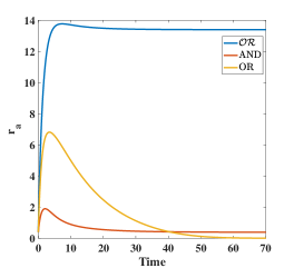
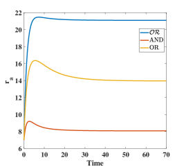
We wanted to investigate whether the absence of the leakage rate of will have any impact on the model dynamics. To understand that, we compared the mRNA concentration for the model systems (1), (8) and (14) for the zero and non-zero values of as shown in Fig. 17 (a) and (b), respectively. From Fig. 17, we observed that the level of mRNA concentration is high for the model with type-II logic (model system 14) (blue color curve) and low for the model with type-I OR logic (model system 1) (orange color curve). Also, it is evident that the level of mRNA concentration is high for all the three model systems with non-zero (Fig. 17b) compared to case (Fig. 17a). However, the structure of the time-dynamics curves of mRNA concentration remains largely unaltered. Our results thus show that leakage only plays the role of ”scaling” in the model and its incorporation in the model systems won’t have any impact on the overall qualitative dynamics of the network. We thus conclude that our results hold true even when the leakage is completely ignored.
.
7 Discussion and Final Conclusion
Cell fate switching is a dynamic phenomenon often tied to regulatory network motifs that at the cellular level define the computational machinery of life. Most of these network motifs define molecular switches exhibiting diverse qualitative behaviors such as bistability, catastrophes, and hysteresis [1]. The most prominent examples of molecular switches involving minimal circuitry are the two-component positive feedback network motifs resulting from mutual repression or mutual activation of two genes. Traditional studies have shown that these motifs can exhibit at most bistable dynamics (two stable states or attractors) allowing the system to alternately switch between two states. Further, the underlying cause of bistable dynamics is attributed to multimeric regulation (higher order Hill coefficient), in contrast to monomeric regulation that gives rise to only monostable dynamics. The biological programs underlying cell fate decision-making are however not just restricted to mono-and bistable regimes of dynamics. In fact, higher-order dynamics such as tristability (three stable states/attractors/phenotypes) is now also prominently observed in biological mechanisms. This happens in differentiation programs such as differentiation of naive CD4+ T cells [37] as well as in diseases-inducing processes such as epithelial-mesenchymal transition (EMT) in which non-motile epithelial cells switch to mesenchymal and hybrid epithelial-mesenchymal cell fates which have migratory and invasive traits that often causes metastasis of carcinomas [26]. Nevertheless, the minimal network motif that can exhibit tristability, or for that matter, mon, bi-and tri stability, remains largely unexplored.
In our previous study on networks underlying and driving EMT, we used a “numerical” approach to report that a positive feedback loop formed by mutual repression of two genes, miR200 ( microRNA) and ZEB (mRNA), with one gene, ZEB, self-activated can exhibit tristability. However, this being a microRNA-mRNA circuit involves translational repression and active degradation of ZEB due to micro-RNA, making it a complicated mechanism. We asked whether a generic positive feedback loop formed by mutual repression of two transcription factors (rather than microRNAs and mRNA’s) with an autoloop, can be the minimal circuit to exhibit lower as well as higher-order stability regimes such as mon, bi-and tri stability. While small feedback circuits with and without delays have been studied previously [38, 39, 40, 41, 42, 43, 44], we still lack answers with rigorous analytical foundations to the following crucial questions: (a) How is multimerization associated with the order of stability? (b) Does the “logic” of regulation have any functional role in multistability? In this work, we address these questions using a rigorous analytical (and numerical) approach that allows us to reach the following conclusions summarised in Table 4.
We show that a positive feedback loop with an autoloop can exhibit diverse dynamical behaviors that depend on the degree of multimerization as well as the “logic” of regulation. The autoloop can be integrated into the core circuit through three types of logic gates: OR (Type-I and Type-II), and AND. With Type-I OR logic, the monomeric circuit with monomeric autoloop can show biphasic kinetics as well as hysteresis (bistability). However, with AND and Type-II logics the circuit can show hyperbolic saturation kinetics - a manifestation of monostability. We show that the necessary geometrical constraint for hysteresis (bistability) with AND and Type-II logics imposes the existence of (at least) dimeric autoloop. We also analyzed higher degrees of multimerization and reported the prevalence of biphasic as well as mono-and bistable dynamics. Finally, and strikingly, we show the possibility of tristability in this circuit. The two requirements for tistable dynamics are: (a) the degrees of multimerization for the two regulations in the core circuit should be (at least) two and three, (b) the degree of multimerization of autoloop should be (at least) two (i. e., dimeric). Taken together, our analysis shows how different multimerization and logical constraints in this minimal circuit can work together to produce numerous types of dynamical scenarios including monostability, hysteresis (bistability), biphasic kinetics, and importantly, tristability. While hysteresis translates to forced and abrupt cell state transitions, biphasic kinetics explains without a step-like switch. The biological network (i.e., miR200-ZEB circuit) corresponding to this generic circuit underlies EMT, and drives cell fate transition and metastasis in carcinomas [45]. Besides, it has been shown (experimentally) to exhibit hysteric as well non-hysteric dynamics, with only the hysteric EMT enabling lung metastasis [46], our results can thus have crucial implications in furthering our understanding of EMT mechanism due to miR200-ZEB feedback loop and can provide inputs to control cell-fate switching during metastasis of carcinomas.
| Type-I OR logic | AND logic | Type-II logic | ||||||||||||
| Monostable |
|
Tristable | Monostable |
|
Tristable | Monostable |
|
Tristable | ||||||
| (1,1,1) | - | - | - | - | - | |||||||||
| (1,1,2) | - | - | - | |||||||||||
| (2,1,2) | - | - | - | |||||||||||
| (2,2,1) | - | - | - | |||||||||||
| (2,2,2) | - | - | - | |||||||||||
| (2,3,2) | - | - | ||||||||||||
| (3,3,3) | - | - | ||||||||||||
Author Contributions
MR: Conceptualization, supervision, funding acquisition. AS: Analytical calculations and numerical simulations. Both authors analysed the data, discussed the results, and wrote the manuscript.
Acknowledgments
This work is supported by the Department of Science and
Technology, India [Grant No. DST/INSPIRE/04/2020/001492] and the Science and Engineering Research Board, India [Grant No. CRG/2023/006432] to Mubasher Rashid.
References
- [1] M Sáez, J Briscoe, and David A Rand. Dynamical landscapes of cell fate decisions. Interface focus, 12(4):20220002, 2022.
- [2] Joseph X Zhou and Sui Huang. Understanding gene circuits at cell-fate branch points for rational cell reprogramming. Trends in genetics, 27(2):55–62, 2011.
- [3] Laura Prochazka, Yaakov Benenson, and Peter W Zandstra. Synthetic gene circuits and cellular decision-making in human pluripotent stem cells. Current Opinion in Systems Biology, 5:93–103, 2017.
- [4] Gábor Balázsi, Alexander Van Oudenaarden, and James J Collins. Cellular decision making and biological noise: from microbes to mammals. Cell, 144(6):910–925, 2011.
- [5] Raúl Guantes and Juan F Poyatos. Multistable decision switches for flexible control of epigenetic differentiation. PLoS computational biology, 4(11):e1000235, 2008.
- [6] Dasong Huang and Ruiqi Wang. Exploring the mechanisms of cell reprogramming and transdifferentiation via intercellular communication. Physical Review E, 102(1):012406, 2020.
- [7] Shubham Tripathi, Herbert Levine, and Mohit Kumar Jolly. The physics of cellular decision making during epithelial-mesenchymal transition. Annual Review of Biophysics, 49:1–18, 2020.
- [8] Shubham Tripathi, Priyanka Chakraborty, Herbert Levine, and Mohit Kumar Jolly. A mechanism for epithelial-mesenchymal heterogeneity in a population of cancer cells. PLoS computational biology, 16(2):e1007619, 2020.
- [9] Dandan Li, Lingyun Xia, Pan Huang, Zidi Wang, Qiwei Guo, Congcong Huang, Weidong Leng, and Shanshan Qin. Heterogeneity and plasticity of epithelial–mesenchymal transition (emt) in cancer metastasis: Focusing on partial emt and regulatory mechanisms. Cell proliferation, 56(6):e13423, 2023.
- [10] Meredith S Brown, Behnaz Abdollahi, Owen M Wilkins, Hanxu Lu, Priyanka Chakraborty, Nevena B Ognjenovic, Kristen E Muller, Mohit Kumar Jolly, Brock C Christensen, Saeed Hassanpour, et al. Phenotypic heterogeneity driven by plasticity of the intermediate emt state governs disease progression and metastasis in breast cancer. Science advances, 8(31):eabj8002, 2022.
- [11] Mubasher Rashid, Kishore Hari, John Thampi, Nived Krishnan Santhosh, and Mohit Kumar Jolly. Network topology metrics explaining enrichment of hybrid epithelial/mesenchymal phenotypes in metastasis. PLOS Computational Biology, 18(11):e1010687, 2022.
- [12] Javier Macía, Stefanie Widder, and Ricard Solé. Why are cellular switches boolean? general conditions for multistable genetic circuits. Journal of theoretical biology, 261(1):126–135, 2009.
- [13] Marcelline Kaufman, Christophe Soule, and René Thomas. A new necessary condition on interaction graphs for multistationarity. Journal of theoretical biology, 248(4):675–685, 2007.
- [14] David Angeli, James E Ferrell Jr, and Eduardo D Sontag. Detection of multistability, bifurcations, and hysteresis in a large class of biological positive-feedback systems. Proceedings of the National Academy of Sciences, 101(7):1822–1827, 2004.
- [15] German Enciso and Eduardo D Sontag. Monotone systems under positive feedback: multistability and a reduction theorem. Systems & control letters, 54(2):159–168, 2005.
- [16] David Angeli and Eduardo D Sontag. Multi-stability in monotone input/output systems. Systems & Control Letters, 51(3-4):185–202, 2004.
- [17] Christophe Soulé. Graphic requirements for multistationarity. ComPlexUs, 1(3):123–133, 2003.
- [18] Timothy S Gardner, Charles R Cantor, and James J Collins. Construction of a genetic toggle switch in escherichia coli. Nature, 403(6767):339–342, 2000.
- [19] Qing Zhou, Hiram Chipperfield, Douglas A Melton, and Wing Hung Wong. A gene regulatory network in mouse embryonic stem cells. Proceedings of the National Academy of Sciences, 104(42):16438–16443, 2007.
- [20] Ahmadreza Ghaffarizadeh, Nicholas S Flann, and Gregory J Podgorski. Multistable switches and their role in cellular differentiation networks. BMC bioinformatics, 15:1–13, 2014.
- [21] Jinfang Zhu, Hidehiro Yamane, and William E Paul. Differentiation of effector cd4 t cell populations. Annual review of immunology, 28:445–489, 2009.
- [22] Atchuta Srinivas Duddu, Sarthak Sahoo, Souvadra Hati, Siddharth Jhunjhunwala, and Mohit Kumar Jolly. Multi-stability in cellular differentiation enabled by a network of three mutually repressing master regulators. Journal of the Royal Society Interface, 17(170):20200631, 2020.
- [23] Laurane De Mot, Didier Gonze, Sylvain Bessonnard, Claire Chazaud, Albert Goldbeter, and Geneviève Dupont. Cell fate specification based on tristability in the inner cell mass of mouse blastocysts. Biophysical journal, 110(3):710–722, 2016.
- [24] En Li. Chromatin modification and epigenetic reprogramming in mammalian development. Nature Reviews Genetics, 3(9):662–673, 2002.
- [25] Mingyang Lu, Mohit Kumar Jolly, Ryan Gomoto, Bin Huang, Jose Onuchic, and Eshel Ben-Jacob. Tristability in cancer-associated microrna-tf chimera toggle switch. The journal of physical chemistry B, 117(42):13164–13174, 2013.
- [26] Mingyang Lu, Mohit Kumar Jolly, Herbert Levine, José N Onuchic, and Eshel Ben-Jacob. Microrna-based regulation of epithelial–hybrid–mesenchymal fate determination. Proceedings of the National Academy of Sciences, 110(45):18144–18149, 2013.
- [27] Mubasher Rashid, Brasanna M Devi, and Malay Banerjee. Combinatorial cooperativity in mir200-zeb feedback network can control epithelial-mesenchymal transition. Bulletin of Mathematical Biology, 86(5):1–23, 2024.
- [28] Vijay Chickarmane, Carl Troein, Ulrike A Nuber, Herbert M Sauro, and Carsten Peterson. Transcriptional dynamics of the embryonic stem cell switch. PLoS computational biology, 2(9):e123, 2006.
- [29] Daniel Huang, William J Holtz, and Michel M Maharbiz. A genetic bistable switch utilizing nonlinear protein degradation. Journal of biological engineering, 6:1–13, 2012.
- [30] Joshua L Cherry and Frederick R Adler. How to make a biological switch. Journal of theoretical biology, 203(2):117–133, 2000.
- [31] Jules Guilberteau, Camille Pouchol, and Nastassia Pouradier Duteil. Monostability and bistability of biological switches. Journal of Mathematical Biology, 83(6):65, 2021.
- [32] Jie Li and Weinian Zhang. Transition between monostability and bistability of a genetic toggle switch in escherichia coli. Discrete & Continuous Dynamical Systems-Series B, 25(5), 2020.
- [33] Simone Brabletz and Thomas Brabletz. The zeb/mir-200 feedback loop—a motor of cellular plasticity in development and cancer? EMBO reports, 11(9):670–677, 2010.
- [34] Alexandra C Title, Sue-Jean Hong, Nuno D Pires, Lynn Hasenöhrl, Svenja Godbersen, Nadine Stokar-Regenscheit, David P Bartel, and Markus Stoffel. Genetic dissection of the mir-200–zeb1 axis reveals its importance in tumor differentiation and invasion. Nature communications, 9(1):4671, 2018.
- [35] Menghan Chen and Ruiqi Wang. Computational analysis of synergism in small networks with different logic. Journal of Biological Physics, 49(1):1–27, 2023.
- [36] Lawrence Perko. Differential equations and dynamical systems. 2013.
- [37] Jinfang Zhu, Hidehiro Yamane, and William E Paul. Differentiation of effector cd4 t cell populations. Annual review of immunology, 28:445–489, 2009.
- [38] Guiyuan Wang, Zhuoqin Yang, and Marc Turcotte. Dynamic analysis of the time-delayed genetic regulatory network between two auto-regulated and mutually inhibitory genes. Bulletin of Mathematical Biology, 82:1–30, 2020.
- [39] Hongguang Xi and Marc Turcotte. Parameter asymmetry and time-scale separation in core genetic commitment circuits. Quantitative Biology, 3:19–45, 2015.
- [40] Kiresh Parmar, Konstantin B Blyuss, Yuliya N Kyrychko, and Stephen John Hogan. Time-delayed models of gene regulatory networks. Computational and mathematical methods in medicine, 2015, 2015.
- [41] Dongya Jia, Mohit Kumar Jolly, William Harrison, Marcelo Boareto, Eshel Ben-Jacob, and Herbert Levine. Operating principles of tristable circuits regulating cellular differentiation. Physical biology, 14(3):035007, 2017.
- [42] Kishore Hari, Pradyumna Harlapur, Aditi Gopalan, Varun Ullanat, Atchuta Srinivas Duddu, and Mohit Kumar Jolly. Emergent properties of coupled bistable switches. Journal of Biosciences, 47(4):81, 2022.
- [43] David S Glass, Xiaofan Jin, and Ingmar H Riedel-Kruse. Nonlinear delay differential equations and their application to modeling biological network motifs. Nature communications, 12(1):1788, 2021.
- [44] Qing Hu, Min Luo, and Ruiqi Wang. Identifying critical regulatory interactions in cell fate decision and transition by systematic perturbation analysis. Journal of Theoretical Biology, 577:111673, 2024.
- [45] Alexandra C Title, Sue-Jean Hong, Nuno D Pires, Lynn Hasenöhrl, Svenja Godbersen, Nadine Stokar-Regenscheit, David P Bartel, and Markus Stoffel. Genetic dissection of the mir-200–zeb1 axis reveals its importance in tumor differentiation and invasion. Nature communications, 9(1):4671, 2018.
- [46] T Celià-Terrassa, C Bastian, DD Liu, B Ell, NM Aiello, Y Wei, J Zamalloa, AM Blanco, X Hang, D Kunisky, et al. Hysteresis control of epithelial-mesenchymal transition dynamics conveys a distinct program with enhanced metastatic ability. nat commun. 2018; 9: 5005.