Optimal Controller Realizations against False Data Injections in Cooperative Driving

Abstract

To enhance the robustness of cooperative driving to cyberattacks, we study a controller-oriented approach to mitigate the effect of a class of False-Data Injection (FDI) attacks. By reformulating a given dynamic Cooperative Adaptive Cruise Control (CACC) scheme (the base controller), we recognize that the base controller can be represented by a class of new but equivalent controllers (base controller realizations) that exhibits the same platooning behavior with varying robustness in the presence of attacks. We propose a prescriptive synthesis framework where the base controller and the system dynamics are written in new coordinates via an invertible coordinate transformation on the controller state. Because the input-output behavior is invariant under coordinate transformations, the input-output behavior is unaffected (so controller realizations do not change the system’s closed-loop performance). However, each base controller realization may require a different combination of sensors. To this end, we obtain the optimal combination of sensors that minimizes the effect of FDI attacks by solving a Linear Matrix Inequality (LMI), while quantifying the FDI’s attack impact through reachability analysis. Through simulation studies, we demonstrate that this approach enhances the robustness of cooperative driving, without relying on a detection scheme and maintaining all system properties.

I INTRODUCTION

Cooperative Adaptive Cruise Control (CACC) is a well-explored technology within Connected and Automated Vehicles (CAVs) that allows groups of vehicles to form tightly-coupled platoons by exchanging inter-vehicle data through Vehicle-to-Vehicle (V2V) wireless communication networks [2]-[4]. However, as CACC requires the use of communication networks, the system exposes network access points that adversaries can exploit for cyberattacks [5]-[8]. To counter these attacks, new technologies are being developed to enhance the prevention and detection of cyberattacks, and so increase system security [7]-[10]. However, the effectiveness of current mitigation technology is limited by: (i) unknown process or measurement disturbances [11, 12], (ii) limited operating resources (e.g., computing power, budget) [13], and (iii) adversaries exploiting model knowledge [13, 14]. Therefore, there is a need for technology that enhances the robustness of cooperative driving to attacks on system elements such as sensors, actuators, networks, and software.

To tackle these challenges, there are two main control-theoretic formulations in the literature: (i) active methods that leverage detection to switch controllers, and (ii) passive attack-resilient methods that seek to withstand the effect of attacks. The former relies on a detection scheme to notify the controller to subsequently switch towards a fallback mechanism (e.g., from CACC to adaptive cruise control [15]), while the latter often compromises the nominal performance (e.g., string stability [16]).

In this paper, we introduce a third controller-oriented approach to implement a given dynamic CACC scheme without affecting the input-output behavior of the closed-loop system, thereby preserving nominal performance. By reformulating the dynamic CACC scheme (the base controller), we recognize that the base controller can be represented by a class of equivalent realizations (base controller realization), having equivalent nominal behavior with varying robustness in the presence of attacks. This approach enhances the robustness of cooperative driving, without relying on a detection scheme and maintaining system properties like string stability.

We demonstrate that a different controller realization may require a different combination of sensors from a set of given sensors, which could be subject to a resource-limited FDI attack. The effect of such an FDI attack can be quantified using reachability analysis to obtain the adversarial reachable set, which provides insight into the size of the state space portion that can be induced by the FDI attack [17]. To this end, we formulate a Semi-Definite Program (SDP) to obtain the optimal controller realization that minimizes the size of the adversarial reachable set. Moreover, the corresponding synthesis problem results is an LMI problem. To support our claims, a simulation study is conducted, where the original CACC realization, an alternative formulation, and the optimal realization are compared. Our findings reveal that the optimal realization has the smallest size of the reachable set within the considered class of controllers.

The structure of the paper is as follows: Section II introduces some preliminary results necessary for the subsequent sections. Section III describes the general problem setting, including the platooning dynamics, the dynamic CACC scheme, and the available measurements. Section IV presents the class of controllers that can be derived from the given problem setting, after which the optimization problem is introduced. Section V presents the optimal realization, and an extensive simulation study is conducted to demonstrate its performance. Finally, Section VI provides the concluding remarks.

II Mathematical Preliminaries

II-A Notation

The symbol $\mathbb{R}$ stands for the real numbers, $\mathbb{R}_{>0}$($\mathbb{R}_{\geq 0}$) denotes the set of positive (non-negative) real numbers. The symbol $\mathbb{N}$ stands for the set of natural numbers, including zero. The $n\times m$ matrix composed of only zeros is denoted by $\mathbf{0}_{n\times m}$, or simply $\mathbf{0}$ when its dimension is clear. Consider a finite index set $\mathcal{L}:=\{l_{1},\ldots,l_{\rho}\}\subset\mathbb{N}$ with cardinality $\text{card}[\mathcal{L}]=\rho$, e.g., $\mathcal{L}=\{1,3,7,15\}$ with $\text{card}[\mathcal{L}]=4$, the notation diag[$B_{j}$] and $(B_{j})$, $j\in\mathcal{L}$, stand for the diagonal block matrix $\text{diag}[B_{l_{1}},\ldots,B_{l_{\rho}}]$ and stacked block matrix $(B_{l_{1}},\ldots,B_{l_{\rho}})$, respectively. The notation $A\geq 0$ (resp., $A\leq 0$) indicates that the matrix $A$ is positive (resp., negative) semidefinite, i.e., all the eigenvalues of the symmetric matrix $A$ are positive (resp. negative) or equal to zero, whereas the notation $A>0$ (resp., $A<0$) indicates the positive (resp., negative) definiteness, i.e., all the eigenvalues are strictly positive (resp. negative). We often omit implicit time dependencies of signals for simplicity of notation.

II-B Definitions and Preliminary Results

Definition 1 (Reachable Set).

[17] Consider the perturbed Linear Time-Invariant (LTI) system:

$$\zeta(k+1)=\mathcal{A}\zeta(k)+\sum_{i=1}^{N}\mathcal{B}_{i}\omega_{i}(k),\ \zeta(0)=\zeta_{0}$$ (1)

with $k\in\mathbb{N}$, state $\zeta(k)\in\mathbb{R}^{n_{\zeta}}$, perturbation $\omega_{i}\in\mathbb{R}^{p_{i}}$ satisfying $\omega_{i}^{\top}W_{i}\omega_{i}\leq 1$ for some positive definite matrix $W_{i}\in\mathbb{R}^{p_{i}\times p_{i}},i=\{1,...,N\},N\in\mathbb{N}$, and matrices $\mathcal{A}\in\mathbb{R}^{n_{\zeta}\times n_{\zeta}}$ and $\mathcal{B}_{i}\in\mathbb{R}^{n_{\zeta}\times p_{i}}$. The reachable set $\mathcal{R}^{\zeta}$(k) at time $k\geq 0$ from the initial condition $\zeta_{0}\in\mathbb{R}^{n_{\zeta}}$ is the set of states reachable in $k$ steps by system (1) through all possible disturbances satisfying $\omega_{i}^{\top}W_{i}\omega_{i}\leq 1$, i.e.,

$$\mathcal{R}^{\zeta_{0}}(k)\!\coloneqq\!\!\left\{\zeta\in\mathbb{R}^{n_{\zeta}}\left|\begin{array}[]{l}\zeta=\zeta(k),\zeta(k)\text{ {solution to \eqref{eq:LTI_set},}}\\ \text{ {and} }\omega_{i}(k)^{\top}W_{i}\omega_{i}(k)\leq 1,\end{array}\!\!\!\!\!\right\}\right..$$ (2)

Lemma 1 (Ellipsoidal Approximation).

[17] Consider the perturbed LTI system (1) and the reachable set $\mathcal{R}^{\zeta}(k)$ in Definition 1. For a given $a\in(0,1)$, if there exist constants $a_{1}$, $\ldots$, $a_{N}$ and matrix $P$ that is the solution of the convex program:

$$\left\{\!\begin{aligned} &\min_{P,a_{1},\ldots,a_{N}}-\log\det[P],\\ &\text{\emph{s.t.}}\hskip 2.84526pta_{1},\ldots,a_{N}\in(0,1),\hskip 1.42262pta_{1}+\ldots+a_{N}\geq a,\\ &P>0,\begin{bmatrix}aP&\mathcal{A}^{\top}P&\mathbf{0}\\ P\mathcal{A}&P&P\mathcal{B}\\ \mathbf{0}&\mathcal{B}^{\top}P&W_{a}\end{bmatrix}\geq 0,\end{aligned}\right.$$ (3)

with matrices $W_{a}:=\operatorname*{diag}\begin{bmatrix}(1-a_{1})W_{1},\ldots,(1-a_{N})W_{N}\end{bmatrix}\in\mathbb{R}^{\bar{p}\times\bar{p}}$ and $\mathcal{B}:=(\mathcal{B}_{1},\ldots,\mathcal{B}_{N})\in\mathbb{R}^{n_{\zeta}\times\bar{p}}$, and $\bar{p}=\sum_{i=1}^{N}p_{i}$; then, for all $k\in\mathbb{N}$, $\mathcal{R}^{\zeta}(k)\subseteq\mathcal{E}^{\zeta}(k)$ with $\mathcal{E}^{\zeta}(k):=\{\zeta^{\top}(k)P^{\zeta}\zeta(k)\leq\alpha^{\zeta}(k)\}$, with convergent scalar sequence $\alpha^{\zeta}(k):=a^{k-1}\zeta(k)^{\top}P\zeta(k)+((N-a)(1-a^{k-1}))/(1-a)$. Ellipsoid $\mathcal{E}^{\zeta}(k)$ has the minimum asymptotic volume among all outer ellipsoidal approximations of $\mathcal{R}^{\zeta}(k)$.

Lemma 2.

[17] For any positive definite matrix $Y\in\mathbb{R}^{n\times n}$, the following is satisfied

$$\det[Y]^{\tfrac{1}{n}}\leq\frac{1}{n}\operatorname*{tr}[Y]\implies\det[Y]^{\tfrac{1}{2}}\leq\frac{1}{n^{\tfrac{n}{2}}}\operatorname*{tr}[Y]^{\tfrac{n}{2}}.$$ (4)

Moreover, because $Y$ is positive definite

$$\operatorname*{arg\,min}[\operatorname*{tr}[Y]^{\tfrac{n}{2}}]=\operatorname*{arg\,min}[\operatorname*{tr}[Y]];$$ (5)

that is, $\operatorname*{tr}[Y]^{\tfrac{n}{2}}$ and $\operatorname*{tr}[Y]$ share the same minimizer. Therefore, by minimizing $\operatorname*{tr}[Y]$, we minimize an upper bound on $\sqrt{\det[Y]}$.

Lemma 3 (Projection).

[17] Consider the ellipsoid:

$$\begin{split}\mathcal{E}:=\left\{x\in\mathbb{R}^{n},y\in\mathbb{R}^{m}\bigg{|}\begin{bmatrix}x\\ y\end{bmatrix}^{\top}\begin{bmatrix}Q_{1}&Q_{2}\\ Q_{2}^{\top}&Q_{3}\end{bmatrix}\begin{bmatrix}x\\ y\end{bmatrix}=\alpha\right\},\end{split}$$ (6)

for some positive definite matrix $Q\in\mathbb{R}^{(n+m)\times(n+m)}$ and constant $\alpha\in\mathbb{R}_{>0}$. The projection $\mathcal{E}^{\prime}$ of $\mathcal{E}$ onto the $x$-hyperplane is given by the ellipsoid:

$$\mathcal{E}^{\prime}:=\left\{x\in\mathbb{R}^{n}\left|\hskip 2.84526ptx^{\top}\begin{bmatrix}Q_{1}-Q_{2}Q_{3}^{-1}Q_{2}^{\top}\end{bmatrix}x=\alpha\right\}.\right.$$ (7)

III Problem Setting

Consider a homogeneous platoon of $m$ vehicles, schematically depicted in Fig. 1, where the vehicles are enumerated with index $i=1,...,m,$ with $i=1$ indicating the lead vehicle. To model such a platoon, we adopt the longitudinal vehicle model from [3], where the dynamics are described by

$$\begin{bmatrix}\dot{d}_{i}\\ \dot{v}_{i}\\ \dot{a}_{i}\end{bmatrix}=\begin{bmatrix}v_{i-1}-v_{i}\\ a_{i}\\ -\frac{1}{\tau}a_{i}+\frac{1}{\tau}u_{i}\end{bmatrix},\,i\in S_{m}\backslash\{1\},$$ (8)

where $d_{i}=q_{i-1}-q_{i}-L_{i}$ ($q_{i}$ reflects the position of the rear bumper of vehicle $i$ and $L_{i}$ its length) being the distance between vehicle $i$ and its preceding vehicle $i-1$, $v_{i}$, and $a_{i}$ denoting the velocity, and acceleration of vehicle $i$, respectively, and $S_{m}\coloneqq\{i\in\mathbb{N}\mid 1\leq i\leq m\}$ (i.e., the set of all vehicles in a platoon of length $m\in\mathbb{N}$). The desired acceleration $u_{i}$ represents the control input, and $\tau>0$ is a time constant modeling driveline dynamics.

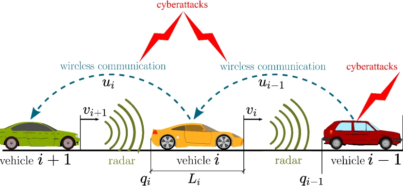
Figure 1: CACC-equipped vehicle platoon. Each vehicle is equipped with onboard sensors (e.g., radars/LiDARs, cameras, and velocity/acceleration sensors). Vehicles may be subject to FDI attacks.

The objective of each follower vehicle is to keep a desired distance $d_{r,i}$ (the so-called constant time-gap policy) with its preceding vehicle:

$$d_{r,i}=r+hv_{i},\,i\in S_{m}\backslash\{1\},$$ (9)

with the time gap $h>0$, and standstill distance $r>0$. The spacing error is then defined as

$$\begin{split}e_{i}&\coloneqq d_{i}-d_{r,i}.\end{split}$$ (10)

To obtain the desired error dynamics, in [2] a CACC controller is introduced to achieve string-stable vehicle-following behavior at small inter-vehicle distances for a homogeneous platoon. This CACC controller is a dynamic controller of the following form:

$$\mathcal{C} \coloneqq\left\{\begin{aligned} u_{i}&=\rho_{i},\\ \dot{\rho}_{i}&=-\tfrac{1}{h}\rho_{i}+\tfrac{1}{h}(k_{p}e_{i}+k_{d}\dot{e}_{i})+\tfrac{1}{h}u_{i-1},\end{aligned}\right.$$ (11)

which stabilizes the resulting error dynamics in (10). The constants $k_{p}$, and $k_{d}$ are control gains to be designed [2]. An alternative to (11) is the CACC controller introduced in [4], which results in the same control signal $u_{i}$ at the vehicle, but is now also applicable for heterogeneous platoons. This CACC controller is also dynamic and of the following form:

$$\hat{\mathcal{C}} \coloneqq\left\{\begin{aligned} \hat{u}_{i}&=-\tfrac{\tau}{h}\hat{\rho}_{i}+(1-\tfrac{\tau}{h})a_{i}+\tfrac{\tau}{h}a_{i-1},\\ \dot{\hat{\rho}}_{i}&=-\tfrac{1}{\tau}\hat{\rho}_{i}-\tfrac{1}{\tau_{i}}(k_{p}e_{i}+k_{d}\dot{e}_{i}).\end{aligned}\right.$$ (12)

Note that, the real-time realization of any control scheme depends on the available sensors $y_{i,j}$ (sensor number $j$ of vehicle $i$). Considering a combination of sensor data coming from onboard sensors (e.g., LiDAR, radar, cameras, and velocity/acceleration sensors) and wirelessly received data from adjacent vehicles, we assume to have the following sensors to realize $\mathcal{C}$ and $\hat{\mathcal{C}}$

$$y_{i,1} \coloneqq d_{i}+\delta_{i,1},$$ (13a)

$$y_{i,2} \coloneqq v_{i}+\delta_{i,2},$$ (13b)

$$y_{i,3} \coloneqq a_{i}+\delta_{i,3},$$ (13c)

$$y_{i,4} \coloneqq v_{i-1}-v_{i}+\delta_{i,4},$$ (13d)

$$y_{i,5} \coloneqq a_{i-1}+\delta_{i,5},$$ (13e)

$$y_{i,6} \coloneqq u_{i-1}+\delta_{i,6}.$$ (13f)

Herein, $\delta_{i,j}$ models potential false data injection attacks. Sensors $y_{i,1}$ and $y_{i,4}$ provide relative tracking and velocity information, $y_{i,2}$ and $y_{i,3}$ denote the onboard measured velocity and acceleration, while $y_{i,5}$ and $y_{i,6}$ model data received from the preceding vehicle via V2V communication. Using (13), it can be observed that $\mathcal{C}$ requires $y_{i,6}$, whereas $\hat{\mathcal{C}}$ requires $y_{i,5}$. The results in [18] show that these two controller realizations provide the same control signal $u_{i}$ at the vehicle for $\delta_{i,j}=0$, but this is not guaranteed when $\delta_{i,j}\neq 0$.

By applying a linear coordinate transformation to the internal state of the dynamic controller (11), infinite real-time realizations of (11) exist using sensors from (13). Therefore, the problem we address in this paper is to determine the optimal controller realization for (11) to minimize the impact of resource-limited adversaries. Additionally, by minimizing the size of the adversarial reachable set, we select an optimal combination of sensors and the corresponding controller realizations to mitigate the effect of a potential FDI attack.

IV Approach

IV-A Controller Realization

One could interpret the difference between the CACC controllers in (11) and (12) as a coordinate transformation on the internal control variable $\rho_{i}$. Therefore, we propose to find the class of controllers that yields the same control signal $u_{i}$ by applying the following coordinate transformation

$$\bar{\rho}_{i} =\alpha_{i}\rho_{i}+\underbrace{\begin{bmatrix}\beta_{i,1}&\beta_{i,2}&\beta_{i,3}&\beta_{i,4}&\beta_{i,5}&0\end{bmatrix}}_{\beta_{i}}y_{i},$$ (14)

with $\bar{\rho}_{i}$ the new controller state, where we aim to find the best choice for both $\alpha_{i}\in\mathbb{R}$ and $\beta_{i}\in\mathbb{R}^{n_{y}}$ ($n_{y}$ number of measurements) to reduce the impact of FDI attacks. It is important to note that in the coordinate transformation, we set $\beta_{i,6}=0$ (excluding $y_{i,6}$), as this would require information about $\dot{u}_{i-1}$, and thus also knowledge about the control structure of vehicle $i-1$ (and possibly sensor data from vehicle $i-2$).

For the closed-loop system we, adopt the formulation from [4], where it was noted that the resulting closed-loop dynamics, with output $e_{i}$ and input $u_{i}$, has relative degree two. Therefore, we differentiate the output $e_{i}$ twice and then investigate the resulting internal dynamics. To this end, we define the stacked state vector $x=[e_{i}\ \ \dot{e}_{i}\ \ z_{i}\ \ v_{i-1}\ \ a_{i-1}]^{\top}$, where $z_{i}\coloneqq v_{i-1}-v_{i}$ is the internal dynamic state, which is input-to-state stable with respect to $a_{i-1}$ [4]. Using (8) to model vehicle dynamics and (10) as error formulation, we obtain the following platooning dynamics

$$\dot{x} =Ax+B_{1}u_{i}+B_{2}u_{i-1},$$ (15)

where

$$\!\!\!\!\!A\! =\!\!\begin{bmatrix}0&1&0&0&0\\ 0&\frac{1}{h}-\frac{1}{\tau}&\frac{1}{\tau}-\frac{1}{h}&0&1\\ 0&\frac{1}{h}&-\frac{1}{h}&0&1\\ 0&0&0&0&1\\ 0&0&0&0&-\frac{1}{\tau}\end{bmatrix}\!\!,\!B_{1}\!=\!\!\begin{bmatrix}0\\ -\tfrac{h}{\tau}\\ 0\\ 0\\ 0\end{bmatrix}\!\!,\!B_{2}\!=\!\!\begin{bmatrix}0\\ 0\\ 0\\ 0\\ \frac{1}{\tau}\end{bmatrix}\!\!.$$ (16)

Using the base controller in (11), we obtain the closed-loop dynamics

$$\begin{bmatrix}\dot{x}\\ \dot{\rho}_{i}\end{bmatrix} =\underbrace{\begin{bmatrix}A&B_{1}\\ K&-\tfrac{1}{h}\end{bmatrix}}_{\mathcal{A}}\begin{bmatrix}x\\ \rho_{i}\end{bmatrix}+\underbrace{\begin{bmatrix}B_{2}\\ \tfrac{1}{h}\end{bmatrix}}_{\mathcal{B}_{u_{i-1}}}u_{i-1},$$ (17)

with $K=\begin{bmatrix}\tfrac{k_{p}}{h}&\tfrac{k_{d}}{h}&0&0&0\end{bmatrix}$.

The sensor measurements in (13) can be expressed in terms of the closed-loop coordinates and disturbance $u_{i-1}$, as the coordinate transformation from $[d_{i}\ \ v_{i}\ \ a_{i}\ \ v_{i-1}\ \ a_{i-1}]^{\top}$ to $[e_{i}\ \ \dot{e}_{i}\ \ z_{i}\ \ v_{i-1}\ \ a_{i-1}]^{\top}$ is invertible. For $\delta_{i}=0$, we obtain

$$y_{i} =\underbrace{\begin{bmatrix}1&0&-h_{i}&h_{i}&0\\ 0&0&-1&1&0\\ 0&-\tfrac{1}{h}&\tfrac{1}{h}&0&0\\ 0&0&1&0&0\\ 0&0&0&0&1\\ 0&0&0&0&0\end{bmatrix}}_{C}\begin{bmatrix}e_{i}\\ \dot{e}_{i}\\ z_{i}\\ v_{i-1}\\ a_{i-1}\end{bmatrix}+\underbrace{\begin{bmatrix}0\\ 0\\ 0\\ 0\\ 0\\ 1\end{bmatrix}}_{D}u_{i-1}.$$ (18)

Since $[C\ \ D]$ is full rank, we can rewrite (18) as

$$\begin{bmatrix}x\\ u_{i-1}\end{bmatrix} =[C\ \ D]^{-1}y_{i}.$$ (19)

To derive the class of base controller realizations, we first reformulate $\dot{\rho}_{i}$ in (11) using the proposed change of coordinates in (14), resulting in

$$\begin{split}\dot{\rho}_{i}&=-\tfrac{1}{h}\rho_{i}+[K\ \ \tfrac{1}{h}]\begin{bmatrix}x\\ u_{i-1}\end{bmatrix}\\ &=-\tfrac{1}{\alpha_{i}h}\bar{\rho}_{i}+\left([K\ \ \tfrac{1}{h}][C\ \ D]^{-1}+\tfrac{1}{\alpha_{i}h}\beta_{i}\right)y_{i}.\end{split}$$ (20)

The dynamics of $\bar{\rho}_{i}$ are then obtained by differentiating (14),

$$\begin{split}\dot{\bar{\rho}}_{i}&=\alpha_{i}\dot{\rho}_{i}+\beta_{i}\dot{y}_{i}\\ &=\alpha_{i}\dot{\rho}_{i}+\beta_{i}(C\dot{x}+D\dot{u}_{i-1}),\end{split}$$ (21)

where due to the structure of $\beta_{i}$ and $D$ we have that $\beta_{i}D=0$. Substitution of (15) provides that

$$\begin{split}\dot{\bar{\rho}}_{i}&=\alpha_{i}\dot{\rho}_{i}+\beta_{i}C[A\ \ B_{2}]\begin{bmatrix}x\\ u_{i-1}\end{bmatrix}+\beta_{i}CB_{1}u_{i}\\ &=\alpha_{i}\dot{\rho}_{i}+\beta_{i}C[A\ \ B_{2}][C\ \ D]^{-1}y_{i}+\beta_{i}CB_{1}u_{i}.\end{split}$$ (22)

The new formulation of the control input $u_{i}$ is obtained by applying the change of coordinates in (14) to (11), which results in

$$u_{i}\! =\!\tfrac{1}{\alpha_{i}}\bar{\rho}_{i}-\tfrac{1}{\alpha_{i}}\beta_{i}y_{i}.$$ (23a)

Substitution of (20) and (23a) into (22) yields

$$\begin{split}\dot{\bar{\rho}}_{i}&=(\tfrac{1}{\alpha_{i}}\beta_{i}CB_{1}-\tfrac{1}{h})\bar{\rho}_{i}+\left(\left(\alpha_{i}[K\ \ \tfrac{1}{h}]+\right.\right.\\ &\left.\left.\beta_{i}C[A\ \ B_{2}]\right)[C\ \ D]^{-1}\!\!+\!\tfrac{1}{h}\beta_{i}\!-\!\tfrac{1}{\alpha_{i}}\beta_{i}CB_{1}\beta_{i}\right)y_{i}.\end{split}$$ (23b)

As a result, we obtain (23) as the class of equivalent controller realizations of (11), which exhibit equivalent platooning behavior in the attack-free scenario. Notice that for $\alpha_{i}=1,\beta_{i}=0$, and for $\alpha_{i}=-\tfrac{\tau}{h},\beta_{i}=[0\ \ 0\ \ (1-\tfrac{\tau}{h})\ \ 0\ \ \tfrac{\tau}{h}\ \ 0]$, the controller realizations $\mathcal{C}$ and $\hat{\mathcal{C}}$ are obtained, respectively. To this end, (23) is derived for $\delta_{i}=0$ to find all equivalent controller realizations that exhibit the same platooning behavior in the attack-free scenario. However, the change of coordinates affects the combinations of sensors being used, and therefore, also influences the effect of an FDI on the platooning behavior. To model the effect of FDI attacks, we now derive (23) for $\delta_{i}\neq 0$ by reformulating (18)

$$y_{i} =[C\ \ D]\begin{bmatrix}x\\ u_{i-1}\end{bmatrix}+\delta_{i}.$$ (24)

Substitution of (24) into (23) yields the realized controller in presence of attacks,

$$u_{i}\! =\!\tfrac{1}{\alpha_{i}}\bar{\rho}_{i}-\tfrac{1}{\alpha_{i}}\beta_{i}[C\ \ D]\begin{bmatrix}x\\ u_{i-1}\end{bmatrix}-\tfrac{1}{\alpha_{i}}\beta_{i}\delta_{i},$$ (25a)

$$\begin{split}\dot{\bar{\rho}}_{i}\!&=\!(\tfrac{1}{\alpha_{i}}\beta_{i}CB_{1}-\tfrac{1}{h})\bar{\rho}_{i}+\left(\alpha_{i}[K\ \ \tfrac{1}{h}]+\beta_{i}C[A\ \ B_{2}]\right.\\ &\ \ \left.+(\tfrac{1}{h}\beta_{i}-\tfrac{1}{\alpha_{i}}\beta_{i}CB_{1}\beta_{i})[C\ \ D]\right)\begin{bmatrix}x\\ u_{i-1}\end{bmatrix}\\ &\ \ +\left(\left(\alpha_{i}[K\ \ \tfrac{1}{h}]+\beta_{i}C[A\ \ B_{2}]\right)[C\ \ D]^{-1}\right.\\ &\ \ \left.+\tfrac{1}{h}\beta_{i}-\tfrac{1}{\alpha_{i}}\beta_{i}CB_{1}\beta_{i}\right)\delta_{i}.\end{split}$$ (25b)

When deriving the closed-loop system using (25), the system matrices $\bar{\mathcal{A}}(\alpha_{i},\beta_{i})$ and $\bar{\mathcal{B}}_{u_{i-1}}(\alpha_{i},\beta_{i})$ (i.e. $-\tfrac{1}{\alpha_{i}}\beta_{i}CB_{1}\beta_{i})[C\ \ D]$ in (25)) are dependent on the choice of $\alpha_{i}$ and $\beta_{i}$. Although different sensors are used, the realization does not affect the nominal closed-loop behavior as the input-output behavior is invariant under coordinate transformations. Therefore, after selecting the required combination of sensors (including $\delta_{i}$), the closed-loop system is transformed back to its original coordinates $[x\ \ \rho_{i}]^{\top}$. As a result: (i) a fair analysis is made between different realizations, as $\mathcal{{A}}$ and $\mathcal{B}_{u_{i-1}}$ are independent, and only $\mathcal{B}_{\delta_{i}}$ is dependent on $\alpha_{i}$ and $\beta_{i}$, and (ii) the resulting dynamics are affine in $\tfrac{1}{\alpha_{i}}\beta_{i}$, allowing for linear and convex optimization techniques, whereas solving it in the new coordinates requires nonlinear optimization techniques. To prove the latter, note that the proposed change of coordinates in (14) is invertible, namely we have that

$$\begin{bmatrix}x\\ \bar{\rho}_{i}\end{bmatrix} =\begin{bmatrix}I&0\\ \beta_{i}C&\alpha_{i}\end{bmatrix}\begin{bmatrix}x\\ \rho_{i}\end{bmatrix}.$$ (26)

By applying the inverse coordinate transformation on the closed-loop (25) (so back to the original closed-loop system (17)), we not only retrieve the original closed-loop formulation, but also obtain the matrix that represents a potential FDI on the closed-loop system

$$\begin{bmatrix}\dot{x}\\ \dot{\rho}_{i}\end{bmatrix} =\mathcal{A}\begin{bmatrix}x\\ \rho_{i}\end{bmatrix}+\mathcal{B}_{u_{i-1}}u_{i-1}+\mathcal{B}_{\delta_{i}}\delta_{i},$$ (27a)

where

$$\!\!\!\!\mathcal{B}_{\delta_{i}}\! =\!\!\begin{bmatrix}-\tfrac{1}{\alpha_{i}}B_{1}\beta_{i}\\ \left([K\ \ \tfrac{1}{h}]\!+\!\tfrac{1}{\alpha_{i}}\beta_{i}C[A\ \ B_{2}]\right)\![C\ \ D]^{-1}\!\!+\tfrac{1}{h\alpha_{i}}\beta_{i}\end{bmatrix}\!\!.$$ (27b)

Note that, as we convert the system back to its original coordinates, only the attack matrix $\mathcal{B}_{\delta_{i}}$ is affected by the choice of $\alpha_{i}$ and $\beta_{i}$. In the following section, we introduce an optimization scheme to find the optimal realization of the base controller within the suggested class of realized controllers.

IV-B Optimization Problem

When looking for the optimal controller realization, we aim to minimize the reachable set induced by resource-limited FDI attacks, which manipulate sensing, actuation, and networked data while being constrained by physical limitations, computing power, and attack strategy [12]. We use the volume of these reachable sets as a security metric, whereas minimizing the volume directly minimizes the size of the state space portion that can be induced by a series of attacks [17]. Computing the exact reachable set is generally not tractable and time-dependent. Instead, we seek to minimize the volume of the outer ellipsoidal approximation.

Computing the reachable set for (27a) is not possible, due to $v_{i-1}$ and $a_{i-1}$ being uncontrollable states, introducing zero-eigenvalues in $\mathcal{A}$. However, note that $v_{i-1}$ and $a_{i-1}$ are fully decoupled (see (17)). Moreover, the choice of $\alpha_{i}$ and $\beta_{i}$ does not affect $v_{i-1}$ and $a_{i-1}$, as the attack only affects the dynamics of $\dot{e}_{i}$ and $\rho_{i}$. Therefore, (27a) is reformulated as

$$\dot{x}_{i} =\mathcal{A}_{i}x_{i}+\mathcal{B}_{i-1}\begin{bmatrix}v_{i-1}\\ a_{i-1}\\ u_{i-1}\end{bmatrix}+B_{i,\delta_{i}}\delta_{i},$$ (28)

where $x_{i}=[e_{i}\ \ \dot{e}_{i}\ \ z_{i}\ \ \rho_{i}]$, and $\mathcal{B}_{i,\delta_{i}}$ as in (27b) but excluding the zero entries for $\dot{v}_{i-1}$ and $\dot{a}_{i-1}$.

In (28) the states and control input of vehicle $i-1$ act as a disturbance on the platooning dynamics. Assuming boundedness of $v_{i-1}$, $a_{i-1}$, and $u_{i-1}$, which is reasonable considering vehicle physical constraints, a reachable set can be found for $\delta_{i}=0$ due to the additional disturbances defined by $\mathcal{B}_{{}_{i-1}}$. However, the ellipsoidal approximation of the reachable set for (28) with $\delta_{i}\neq 0$ can be obtained by the Minkowski sum of two independent ellipsoidal approximation of the reachable induced by $\mathcal{B}_{{}_{i-1}}$ and $\mathcal{B}_{\delta_{i}}$ separately [19]. Therefore, we mitigate the effect of $\mathcal{B}_{{}_{i-1}}$, as the optimal $\alpha_{i}$ and $\beta_{i}$ do not affect this reachable set. Moreover, we are only interested in minimizing the reachable set induced by $\mathcal{B}_{\delta_{i}}$. To this end, for synthesis of the optimal realization, (28) is modeled as it is only perturbed by $\delta_{i}$, resulting in

$$\dot{\tilde{x}}_{i} =\mathcal{A}_{i}\tilde{x}_{i}+\mathcal{B}_{i,\delta_{i}}\delta_{i}.$$ (29)

Note that we use $\tilde{x}_{i}$, to clearly distinguish the platooning dynamics in (28) and (29), as these do not represent the same dynamical system.

Given that the realized controller operates in discrete time, and attacks operate on sampled signals, a discrete-time equivalent model of (29) is obtained via exact discretization at the sampling time instant, $t=T_{s}k,\,k\in\mathbb{N}$, where $T_{s}>0$ is the sampling interval. The resulting discrete-time model can be written as

$$\tilde{x}_{i}(k+1) =\mathcal{A}_{i}^{d}\tilde{x}_{i}(k)+\mathcal{B}^{d}_{i,\delta_{i}}\delta_{i}(k),\ \tilde{x}_{i}(0)=\tilde{x}_{i,0}$$ (30)

with

$$\mathcal{A}_{i}^{d}=e^{\mathcal{A}_{i}T_{s}}, \mathcal{B}^{d}_{i,\delta_{i}}=\left(\int_{0}^{T_{s}}e^{\mathcal{A}_{i}\left(T_{s}-s\right)}ds\right)\mathcal{B}_{i,\delta_{i}}.$$ (31)

The constraints we impose on $\delta_{i}(k)$ have the following structure

$$\delta_{i,j}(k)\in\{\delta_{i,j}\mid\hskip 2.84526pt\delta^{2}_{i,j}\leq W^{2}_{i,j}\},\,\forall k\in\mathbb{N},$$ (32)

for some known constants $W_{i,j}\in\mathbb{R}_{>0},j\in\{1,2,..,6\}$. Associated with these constraints, we introduce the adversarial reachable set (Definition 1)

$$\mathcal{R}^{\tilde{x}_{i,0}}(k):=\left\{\tilde{x}_{i}\in\mathbb{R}^{4}\left|\begin{aligned} &\tilde{x}_{i,0}=\tilde{x}_{i}(k),\\ &\tilde{x}_{i}(k)\text{ solution to }\eqref{eq:CL_ReachableSet2},\\ &\delta_{i}(k)\text{ satisfies }\eqref{eq:DeltaBound}.\end{aligned}\right.\right\}$$ (33)

We seek to obtain the outer ellipsoidal approximation $\mathcal{E}^{\tilde{x}_{i}}(k)$ of $\mathcal{R}^{\tilde{x}_{i}}(k)$ via Lemma 1. Moreover, we have that $\mathcal{E}^{\tilde{x}_{i}}(k)\approx\mathcal{E}^{\tilde{x}_{i}}(\infty)\coloneqq\{\tilde{x}_{i}\mid\tilde{x}_{i}^{\top}\mathcal{P}^{\tilde{x}_{i}}\tilde{x}_{i}\leq(N-a)/(1-a)\}$, for some positive definite matrix $\mathcal{P}^{\tilde{x}_{i}}\in\mathbb{R}^{4\times 4}$, where $N$ represents the number of disturbances, and $a\in(0,1)$. As we consider the reachable set at infinity, the ellipsoidal approximation is independent of the initial condition.

By applying Lemma 1, we can find $\mathcal{P}^{\tilde{x}_{i}}$, where $\mathcal{A}=\mathcal{A}^{d}_{i}$, $\mathcal{B}=\mathcal{B}^{d}_{i,\delta_{i}}$, with $\mathcal{A}^{d}_{i}$ and $\mathcal{B}^{d}_{i,\delta_{i}}$ as formulated in (LABEL:eq:DiscreteSystemMatrices). However, now we aim to minimize $-\log\det[\mathcal{P}^{\tilde{x}_{i}}]$ while also optimizing $\mathcal{B}(\alpha_{i},\beta_{i})$, which results in a non-linear control problem. To this end, we convert the SDP problem in Lemma 1 to a problem formulation that is affine in both $\mathcal{P}^{\tilde{x}_{i}}$ and $\mathcal{B}(\alpha_{i},\beta_{i})$. A congruence transformation of the form $QWQ^{\top}\geq 0$ is applied, where $Q=Q^{\top}=\operatorname*{diag}[(\mathcal{P}^{\tilde{x}_{i}})^{-1},(\mathcal{P}^{\tilde{x}_{i}})^{-1},I]>0$, which preserves the definiteness of the matrix inequality [20]. Applying this congruence transformation to Lemma 1 yields

$$\begin{bmatrix}a(\mathcal{P}^{\tilde{x}_{i}})^{-1}&(\mathcal{P}^{\tilde{x}_{i}})^{-1}(\mathcal{A}_{i}^{d})^{\top}&\mathbf{0}\\ \mathcal{A}_{i}^{d}(\mathcal{P}^{\tilde{x}_{i}})^{-1}&(\mathcal{P}^{\tilde{x}_{i}})^{-1}&\mathcal{B}(\alpha_{i},\beta_{i})\\ \mathbf{0}&(\mathcal{B}(\alpha_{i},\beta_{i}))^{\top}&W_{a}\end{bmatrix} \geq 0.$$ (34)

However, when applying the congruence transformation, the resulting objective function $\min-\log\det[(\mathcal{P}^{\tilde{x}_{i}})^{-1}]$ becomes concave. Instead, we seek to minimize a convex upper bound on $\sqrt{\det[(\mathcal{P}^{\tilde{x}_{i}})^{-1}]}$, which is proportional to the volume of the ellipsoid, from which also the original objective $\log\det[\mathcal{P}^{\tilde{x}_{i}}]$ is derived. To this end, we use Lemma 2 and minimize $\operatorname*{tr}[Y]$, where $Y=(\mathcal{P}^{\tilde{x}_{i}})^{-1}$. Additionally, $\mathcal{B}(\alpha_{i},\beta_{i})$ is affine in $\tfrac{1}{\alpha_{i}}\beta_{i}$, where $\alpha_{i}$ only scales $\beta_{i}$ and hence does not affect the reachable set. Therefore, w.l.o.g. we solve the SDP for $\alpha_{i}=1$. As a result, we obtain

$$\left\{\!\begin{aligned} &\underset{Y,\beta_{i},a_{1},\ldots,a_{N}}{\text{minimize}}\operatorname*{tr}[Y],\\ &\text{\emph{s.t.}}\hskip 2.84526pta_{1},\ldots,a_{N}\in(0,1),\hskip 1.42262pta_{1}+\ldots+a_{N}\geq a,\\ &Y>0,\begin{bmatrix}aY&Y(\mathcal{A}_{i}^{d})^{\top}&\mathbf{0}\\ \mathcal{A}_{i}^{d}Y&Y&\mathcal{B}(\beta_{i})\\ \mathbf{0}&(\mathcal{B}(\beta_{i}))^{\top}&W_{a}\end{bmatrix}\geq 0.\end{aligned}\right.$$ (35)

This minimization is solved in the following section to optimize the realization of $\mathcal{C}$.

V Results

In this section, we solve the optimization problem introduced in $\eqref{eq:OP_OptProblem}$ to determine the optimal realization of (11). We adopt the controller settings from [2], with a desired inter-vehicle distance of $r=3\,$m, with driveline dynamics constant $\tau=0.1\,$s, time headway constant $h=0.5\,$s, and controller gains of $(k_{p},k_{d})=(0.2,0.7)$. The sampling rate is set to $T_{s}=0.01\,$s. For the resource-limited FDI attacks $\delta_{i,j}(k)$, we assume adherence to the bound specified in (32) with $W_{i}=I$, thereby considering potential attacks on all sensors. The bound $W_{i,j}$ is arbitrarily chosen to illustrate the results.

The results are obtained using YALMIP, an open-source toolbox [21], with SDP solver SDPT3 [22]. Setting $\alpha_{i}=1$, we obtain the following optimal realization

$$\!\!\bar{\mathcal{C}}\! \coloneqq\!\left\{\begin{aligned} \bar{u}_{i}&=\!\bar{\rho}_{i}\!+\!0.771y_{i,1}\!-\!0.33y_{i,2}\\ &-0.135y_{i,3}+1.672y_{i,4}+0.187y_{i,5},\\ \dot{\bar{\rho}}_{i}&=-0.65\bar{\rho}_{i}-1.142y_{i,1}+0.46y_{i,2}\\ &\!+\!0.222y_{i,3}\!-\!2.715y_{i,4}\!-\!0.176y_{i,5}\!+\!0.13y_{i,6},\end{aligned}\right.$$ (36)

Notably, the optimal realization $\bar{\mathcal{C}}$ maximizes robustness against $\delta_{i}$ by utilizing all available sensors (18).

In Fig. 2 the outer ellipsoidal approximation of (30) (using Lemma 1) is projected on the $e_{i}$-$z_{i}$ plane (using Lemma 3). These reachable sets are computed for $\delta_{i}\neq 0$ and $W_{i}=I$. Among the three controllers, despite being derived from minimizing the upper bound on the volume, $\bar{\mathcal{C}}$ has the smallest ellipsoidal approximation $(\bar{\mathcal{E}}^{\tilde{x}_{i}})$ in terms of volume, therefore being the most robust realization. However, the projections in Fig. 2 indicate there exists some attack where $\mathcal{C}$ is more robust than $\bar{\mathcal{C}}$, as $\bar{\mathcal{E}}^{\tilde{x}_{i}}\nsubseteq\mathcal{E}^{\tilde{x}_{i}}$.

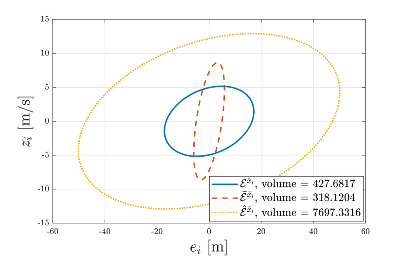
Figure 2: Outer ellipsoidal approximation of the reachable set in (30) for the different controller realizations $\mathcal{C}$, $\bar{\mathcal{C}}$, and $\hat{\mathcal{C}}$. Results are projected onto the $z_{i}$-$e_{i}$ plane, given that $\delta_{i}\neq 0$, and $W_{i}=I$.

As a case study, all three controllers are simulated using MATLAB Simulink. The vehicles are modeled via the platooning dynamics in (8), where the controllers in (11), (12), and (36) are used to control three different platoons. Each platoon consists of a follower (vehicle $i$), which is controlled via one of the realized controllers, whereas the seconder vehicle $i-1$, the leader, is controlled via a simple cruise controller. The leader aims to drive a steady-state velocity of 50 [km/h] while being subject to some traffic in the initial stage, resulting in some transient platooning behavior. Two different scenarios are investigated: (i) vehicle $i$ is subject to a FDI attack on $y_{i,2}$, representing the onboard velocity measurement, where $\delta_{i,2}=\sin(0.01t)\ \forall t\in[20,150]$, and (ii) vehicle $i$ is subject to a FDI attack on $y_{i,3}$, representing the onboard acceleration measurement, where $\delta_{i,3}=\sin(3t)\ \forall t\in[20,75]$.

The results for scenario (i) and scenario (ii) are depicted in Fig. 3 and Fig. 4, respectively. The results show at the initial stage that the different controller realizations exhibit equivalent platooning behavior, as the platooning behavior is invariant under the coordinate transformation. During the FDI in scenario (i), the vehicle controlled by $\bar{\mathcal{C}}$ is the most robust against the attack, as the vehicle states and control input in Fig. 3 show the least magnitude amplification of $\delta_{i,2}$. In scenario (ii), controller $\mathcal{C}$ shows the least magnitude amplification of $\delta_{i,3}$, which corresponds with the results obtained in Fig. 2, showing that this attack is one use-case resulting in $\bar{\mathcal{E}}^{\tilde{x}_{i}}\nsubseteq\mathcal{E}^{\tilde{x}_{i}}$.

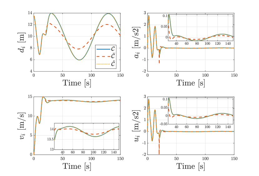
Figure 3: Vehicle and controller response for the different controller realizations $\mathcal{C}$, $\bar{\mathcal{C}}$, and $\hat{\mathcal{C}}$, given an FDI attack on $y_{i,2}$, where $\delta_{i,2}=\sin(0.01t)\ \forall t\in[20,150]$ s.

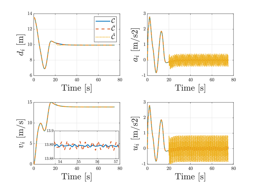
Figure 4: Vehicle and controller response for the different controller realizations $\mathcal{C}$, $\bar{\mathcal{C}}$, and $\hat{\mathcal{C}}$, given an FDI attack on $y_{i,3}$, where $\delta_{i,3}=\sin(3t)\ \forall t\in[20,75]$ s.

VI CONCLUSIONS AND FUTURE WORKS

Cooperative driving must ensure safety and reliability in adversarial environments. To this end, we introduce the choice for a dynamic controller realization as a third controller-oriented approach to enhance the robustness of cooperative driving to cyberattacks. It is shown, that by reformulating a given dynamic CACC scheme, a class of equivalent controller realizations exists, having equivalent nominal behavior with varying robustness in the presence of attacks.

Furthermore, we introduced a framework to find the optimal subset of sensors to realize the controller while jointly minimizing the effect of FDI attacks, which is quantified using reachability analysis. To show our findings, three different CACC realizations are compared, one of which is the optimal realization. The optimal realization is shown to have the smallest reachable set, however, real-time simulations show that there still exists attacks where different realizations are more robust. Hence, a direction of further investigation would be to investigate different optimization strategies to find the best realization. Another line of research concerns controller realization considering a detection scheme, providing a more accurate bound on the FDI attacks.

References

- [1]
- [2] J. Ploeg, B. T. M. Scheepers, van Nunen, N. van de Wouw, and H. Nijmeijer, ”Design and Experimental Evaluation of Cooperative Adaptive Cruise Control”, in IEEE Conference on Intelligent Transportation Systems (ITSC), p. 260–265, 2011.
- [3] J. Ploeg, E. Semsar-Kazerooni, G. Lijster, N. van de Wouw, and H. Nijmeijer, ”Graceful Degradation of CACC Performance Subject to Unreliable Wireless Communication”, in IEEE Conference on Intelligent Transportation Systems (ITSC), p. 1210–1216, 2013.
- [4] E. Lefeber, J. Ploeg, and H. Nijmeijer, ”Cooperative Adaptive Cruise Control of Heterogeneous Vehicle Platoons”, in IFAC-PapersOnLine, vol. 53, no. 2, p. 15217–15222, 2020.
- [5] M. Amoozadeh, A. Raghuramu, C. Chuah, D. Ghosal, M. Zhang, J. Rowe, and K. Levitt, ”Security Vulnerabilities of Connected Vehicle Streams and Their Impact on Cooperative Driving”, in IEEE Communications Magazine, vol. 53, p. 126–132, 2015.
- [6] Z. El-Rewini, K. Sadatsharan, D. F. Selvaraj, S. J. Plathottam, and P. Ranganathan, ”Cybersecurity Challenges in Vehicular Communications”, in Vehicular Communications, vol. 23, p. 100214, 2020.
- [7] Z. Ju, H. Zhang, X. Li, X. Chen, J. Han, and M. Yang, ”A Survey on Attack Detection and Resilience for Connected and Automated Vehicles: From Vehicle Dynamics and Control Perspective,” in IEEE Transactions on Intelligent Vehicles, vol. 7, p. 815–837, 2022.
- [8] X. Sun, F. R. Yu, and Z. Zhang, ”A Survey on Cyber-Security of Connected and Autonomous Vehicles (CAVs)”, in IEEE Transactions on Intelligent Transportation Systems, vol. 23, no. 7, p. 6240–6259, 2022.
- [9] A. Teixeira, I. Shames, H. Sandberg, and K. H. Johansson, ”A Secure Control Framework for Resource-Limited Adversaries, in Automatica, vol. 51, p. 135–148, 2015.
- [10] A. Chowdhury, G. Karmakar, J. Kamruzzaman, A. Jolfaei, and R. Das, ”Attacks on Self-Driving Cars and Their Countermeasures: A Survey”, in IEEE Access, vol. 8, p. 207308–207342, 2020.
- [11] A. Teixeira, D. Pérez, H. Sandberg, and K. H. Johansson, ”Attack models and scenarios for networked control systems”, in Proceedings of the 1st international conference on High Confidence Networked Systems, p. 55-64, 2012.
- [12] X.-M. Zhang, Q.-L Han, X. Ge et al., ”Networked Control Systems: A Survey of Trends and Techniques”, in IEEE/CAA Journal of Automotica Sinica, p. 1-17, 2019.
- [13] S. C. Anand, A. M. H. Teixeira, and A. Ahlen, ”Risk assessment and optimal allocation of security measures under stealthy false data injection attacks”, in 2022 IEEE Conference on Control Technology and Applications (CCTA), p. 1347–-1353, 2022.
- [14] A. Teixeira, H. Sandberg and K. H. Johansson, ”Strategic stealthy attacks: The output-to- output 2-gain”, in 2015 54th IEEE Conference on Decision and Control (CDC), p. 2582–-2587, 2015.
- [15] R. van der Heijden, T. Lukaseder, and F. Kargl, ”Analyzing Attacks on Cooperative Adaptive Cruise Control (CACC)”, in IEEE Vehicular Networking Conference (VNC), p. 45–52, 2017.
- [16] M. Wolf, A. Willecke, J.-C. Muller et al., ”Securing CACC: Strategies for Mitigating Data Injection Attacks”, in 2020 IEEE Vehicular Networking Conference (VNC), p. 1–7, 2020.
- [17] C. Murguia, I. Shames, J. Ruths, and D. Nešić, ”Security metrics and synthesis of secure control systems,” in Automatica, vol. 115, p. 108757, 2020.
- [18] M. Huisman, C. Murguia, E. Lefeber, and N. van de Wouw, ”Impact Sensitivity Analysis of Cooperative Adaptive Cruise Control Against Resource-Limited Adversaries”, in 62nd IEEE Conference on Decision and Control (CDC), p. 5105–5110, 2023.
- [19] A. Halder, ”On the Parameterized Computation of Minimum Volume Outer Ellipsoid of Minkowski Sum of Ellipsoids”, in IEEE Conference on Decision and Control (CDC), p. 4040–4045, 2018.
- [20] S. Boyd, L. El Ghaoi, E. Feron, and V. Balakrishnan, ”Linear Matrix Inequalities in System and Control Theory”, SIAM, 1994.
- [21] J. Lofberg, YALMIP: A Toolbox for Modeling and Optimization in MATLAB, In Proceedings of the CACSD Conference, 2004.
- [22] K.C. Toh, M.J. Todd, and R.H. Tutuncu, SDPT3 — a Matlab software package for semidefinite programming, version 1.3, Optimization Methods and Software, 11 (1999), pp. 545–581.