Nonlinear Model Reduction to
Temporally Aperiodic Spectral Submanifolds

We extend the theory of spectral submanifolds (SSMs) to general non-autonomous dynamical systems that are either weakly forced or slowly varying. Examples of such systems arise in structural dynamics, fluid-structure interactions and control problems. The time-dependent SSMs we construct under these assumptions are normally hyperbolic and hence will persist for larger forcing and faster time dependence that are beyond the reach of our precise existence theory. For this reason, we also derive formal asymptotic expansions that, under explicitly verifiable nonresonance conditions, approximate SSMs and their aperiodic anchor trajectories accurately for stronger, faster or even temporally discontinuous forcing. Reducing the dynamical system to these persisting SSMs provides a mathematically justified model reduction technique for non-autonomous physical systems whose time dependance is moderate either in magnitude or speed. We illustrate the existence, persistence and computation of temporally aperiodic SSMs in mechanical examples under chaotic forcing.

Reduced models for complex physical systems are of growing interest in various areas of applied science and engineering. Mathematically justifiable reduction approaches, such as spectral submanifold (or SSM) reduction, seek to identify the internal dynamics on lower-dimensional, attracting invariant sets in the phase space of the system. These reduced dynamics then become viable reduced models for general trajectories that approach the invariant set and synchronize with its inner motions. SSM reduction also allows for periodic or quasiperiodic time dependence in the full system, but has been inapplicable to systems with more general time dependence, such as impulsive, chaotic or discontinuous forcing. This has hindered applications of SSM reduction to a number of problems in structural dynamics. Here we remove this limitation by extending SSM theory of temporally aperiodic dynamical systems. We obtain exact results for cases of smooth small or smooth slow forcing, but find that our formulas for SSM-reduced dynamics extend to larger and faster forcing in physical examples, including even discontinuous chaotic forcing.

1 Introduction

In its simplest form, a spectral submanifold (SSM) of an autonomous dynamical system is an invariant manifold $W(E)$ that is tangent to a spectral subspace $E$ of the linearized system at a fixed point (Haller and Ponsioen [18]). Classic examples of spectral submanifolds are the stable, unstable and center manifolds tangent to spectral subspaces in which the linearized spectrum has eigenvalues with purely negative, positive and zero real parts, respectively. The stable and unstable manifolds are well known to be unique and as smooth as the dynamical system, while center manifolds are non-unique and not all of them are guaranteed to be as smooth as the dynamical system (Guckenheimer and Holmes [17], Hirsch et al. [23]). Near fixed points that only have eigenvalues with negative and zero real parts, center manifolds attract all trajectories and hence the dynamics restricted to it provides a mathematically exact reduced-order model for the full system (Carr [6], Roberts [42]).

Dissipative physical systems, however, generically have hyperbolic equilibria and hence admit no center manifolds. Instead, near their stable equilibria, such systems tend to have a set of fastest-decaying modes that die out quickly, leaving a set of slower decaying modes to govern the longer-term dynamics. Slow manifolds (i.e., SSMs constructed over such slower decaying modes) then replace center manifolds as targets for mathematically justified model reduction. Such slow SSMs were first targeted via Taylor expansions as nonlinear normal modes (NNMs) by Shaw and Pierre [44]. These insightful calculations were then extended by the same authors to periodically and quasi-periodically forced mechanical systems to approximate forced mechanical response in a number of settings (see, e.g., the reviews by Kerschen et al. [28], Mikhlin and Avramov [33], Touzé et al. [47], Mikhlin and Avramov [32]).

Later mathematical analysis of general SSMs yielded precise existence, uniqueness and smoothness results for these manifolds. Specifically, if the spectral subspace $E$ comprises either only decaying modes or only growing modes (i.e., $E$ is a like-mode spectral subspace) with no integer resonance relationships to the modes outside of $E$, then the slow SSM family $W(E)$ has a unique, primary member, $W^{\infty}(E)$, that is as smooth as the full dynamical system (Cabré et al. [5], Haller and Ponsioen [18]). The remaining secondary (or fractional) members of the SSM family have reduced but precisely known order of differentiability that depends on the ratio of linearized decay rates outside $E$ to those inside $E$ (Haller et al. [19]). If we further disallow any integer resonance in the full linearized spectrum, then primary and fractional SSMs also exist when $E$ is of mixed-mode type, i.e., spanned by a combination of stable and unstable linear modes (Haller et al. [19]).

All these results also hold for discrete autonomous dynamical systems, and hence SSM results also cover time-periodic continuous dynamical systems when applied to their Poincaré maps. Based on this fact, numerical implementations of time-periodic SSM calculations for periodically forced finite-element structures have appeared in Ponsioen et al. [36, 37, 38], Jain and Haller [24], Vizzaccaro et al. [49]. An open source, equation-driven MATLAB toolbox (SSMTool) with a growing collection of worked problems is also available for mechanical systems with general nonlinearities (Jain et al. [25]). Data-driven construction of time-periodic SSMs have been developed and applied to numerical and experimental data by Cenedese et al. [8, 9], Kaszás et al. [26], Axås et al. [3], with open-source MATLAB implementations (SSMLearn and fastSSM) available from Cenedese et al. [7].

Outside autonomous and time-periodic non-autonomous systems, the existence of like-mode SSMs has only been treated under small, time-quasiperiodic perturbations of autonomous dynamical systems (Haro and de la Llave [20], Haller and Ponsioen [18], Opreni et al. [34], Thurner et al. [46]). In such systems, the role of hyperbolic fixed points as anchor points for SSMs is taken over by invariant tori whose dimension is equal to the number of rationally independent frequencies present in the forcing. An SSM in such a case perturbs from the direct product of an unperturbed invariant torus with an underlying spectral subspace $E$. Such SSMs have been shown to exist for like-mode spectral subspaces $E$ under small quasi-periodic perturbations, provided that the real part of the linearized spectrum within $E$ has no integer relationships with the real part of the spectrum outside $E$ (Haro and de la Llave [20], Haro et al. [21], Haller and Ponsioen [18]).

Related work by Fontich et al. [16] covers the persistence and smoothness of primary SSMs emanating from an arbitrary attracting orbit of an autonomous dynamical system. While all non-autonomous systems become autonomous when their phase space is extended with the time variable, this theory does not apply under such an extension. The reason is that all attracting orbits lose hyperbolicity in the extended phase space due to the presence of the neutrally stable time direction.

In summary, while available SSM results have proven highly effective in equation-driven and data-driven reduced-order modeling of autonomous, time-periodic and time-quasiperiodic systems, they offer no theoretical basis or computational scheme for physical systems with general aperiodic time-dependence. Yet the aperiodic setting is clearly of importance in a number of problems, including turbulent fluid-structure interactions, civil engineering structures subject to benchmark aperiodic forcing (such as those mimicking earthquakes) and control of robot motion.

In this paper, we extend available SSMs results to systems with general time dependence. While several powerful linearization results imply the existence of invariant manifolds for such non-autonomous dynamical systems, these results guarantee either no smoothness for SSM-type invariant manifolds (see, e.g., Palmer [35]) or rely on conditions involving the Lyapunov spectra, Sacker–Sell spectra or dichotomy spectra of some associated non-autonomous linear systems of ODEs (see, e.g., Yomdin [50], Pötzsche [39] and Cuong et al. [11]). The latter types of conditions are intuitively clear but not readily verifiable, especially not in a data-driven setting. Here our objective is to conclude the existence of time-aperiodic SSMs under directly computable conditions that also lead to explicitly computable SSM-reduced models in equation-driven and data-driven applications.

To this end, we consider two settings that arise frequently in practice: weak and additive non-autonomous time dependence and slowly varying (or adiabatic) time dependence. The first setting of weak non-autonomous external forcing is common in structural vibrations, wherein a structure’s steady-state response is of interest under various moderate loading scenarios. So far, related studies have been restricted to temporally periodic or quasiperiodic forcing (see, e.g., Ponsioen et al. [36, 37, 38], Li et al. [30, 31], Jain and Haller [24], Vizzaccaro et al. [48], Opreni et al. [34]), because the existence and exact form of a steady state and its associated SSM have been unknown for more general forcing profiles. The second setting of slow time dependence arises, for instance, in controls applications wherein the intended motion of a structure is generally much slower than the characteristic time scales of its internal vibrations. In those applications, the lack of an adiabatic SSM theory has so far confined model-reduction studies to small-amplitude trajectories along which a single, autonomous SSM computed at a nearby fixed point was used for modeling purposes (Alora et al. [1, 2]).

In both of these non-autonomous settings, we use, modify or extend prior invariant manifold results and techniques to conclude the existence of weakly aperiodic or adiabatic SSMs in the limit of small enough or slow enough time dependence, respectively. We then derive explicit recursive formulas for the arising non-autonomous SSMs and the aperiodic anchor trajectories to which they are attached. These formulas also cover and extend temporally periodic and aperiodic SSM computations to arbitrarily high order of accuracy. Using simple mechanical examples subjected to chaotic excitation, we illustrate that the new asymptotic formulas yield accurate reduced-order models even for larger and faster forcing.

2 Non-autonomous SSMs under weak forcing

2.1 Set-up

Consider a non-autonomous dynamical system of the form

$$\dot{x}=Ax+f_{0}(x)+f_{1}(x,t),\quad x\in\mathbb{R}^{n},\quad A\in\mathbb{R}^{n\times n},\quad f_{0}\in C^{r}(U),\quad f_{0}(x)=o\left(\left|x\right|\right),$$ (1)

for some integer $r\geq 0$ and with

$$\left\|f_{1}\right\|_{U}=\sup_{(x,t)\in U\times\mathbb{R}}\left|f_{1}(x,t)\right|<\infty$$ (2)

on a compact neighborhood $U\subset\mathbb{R}^{n}$. We consider system (1) a perturbation of the autonomous system

$$\dot{x}=Ax+f_{0}(x),$$ (3)

that has a fixed point at $x=0$ by our assumptions on $f_{0}(x)$. Both $A$ and $f_{0}(x)$ may additionally depend on parameters, which we will suppress here for notational simplicity but will point out in the statement of our main results. Note that the time-dependent term $f_{1}(x,t)$ is also allowed to depend on the phase space variable $x$. Consequently, in addition to describing purely time-dependent external forcing, $f_{1}(x,t)$ can also capture what is commonly called parametric forcing in the structural vibrations literature, i.e., time-dependence in the internal structure of the system.

We assume that the origin is a hyperbolic fixed point of (3), i.e., all eigenvalues in the spectrum of $A,$

$$\mathrm{spect}\left(A\right)=\left\{\lambda_{1},\ldots,\lambda_{n}\right\},$$ (4)

listed in the order

$$\mathrm{Re}\lambda_{n}\leq\mathrm{Re}\lambda_{n-1}\leq\ldots\leq\mathrm{Re}\lambda_{2}\leq\mathrm{Re}\lambda_{1},$$ (5)

satisfy

$$\mathrm{Re}\lambda_{j}\neq 0,\quad j=1,\ldots,n.$$ (6)

For simplicity of exposition, we assume that $A$ is semisimple and hence has $n$ eigenvectors $e_{1},\ldots,e_{n}\in\mathbb{C}^{n}$ corresponding to the eigenvalues listed in (4). The $k^{th}$ eigenspace $E_{k}$ of $A$ is then the linear span of the real and imaginary parts of the eigenvectors corresponding to the eigenvalue $\lambda_{k}$, i.e.,

$$E_{k}=\mathrm{\underset{\text{A$e_{j}$=$\lambda_{k}e_{j}$}}{span}}\left\{\mathrm{Re\,}e_{j},\mathrm{Im}\,e_{j}\right\}.$$

Note that any such eigenspace in an invariant subspace under the dynamics of the linearized ODE

$$\dot{x}=Ax.$$ (7)

A spectral subspace $E$ is the direct sum of a selected group of $\ell$ eigenspaces, i.e.

$$E=E_{j_{1}}\oplus\ldots\oplus E_{j_{\ell}}.$$ (8)

Two important spectral subspaces are the stable subspace $E^{s}$ and the unstable subspace $E^{u}$, defined as

$$E^{s}=\underset{\mathrm{Re}\lambda_{j}<0}{\oplus}E_{j},\qquad E^{u}=\underset{\mathrm{Re}\lambda_{j}>0}{\oplus}E_{j},\qquad E^{s}\oplus E^{u}=\mathbb{R}^{n}.$$ (9)

At least one of $E^{s}$ and $E^{u}$ is nonempty due to the hyperbolicity assumption (6). As a consequence of this assumption, there exist also constants $K,\kappa>0$ such that

$$\left\|e^{At}|_{E^{s}}\right\|\leq Ke^{-\kappa t},\quad\left\|e^{-At}|_{E^{u}}\right\|\leq Ke^{-\kappa t},\quad t\geq 0.$$ (10)

This property of $A$ is usually referred to as exponential dichotomy. For $\kappa$, we can select any positive number satisfying

$$0<\kappa<\min_{1\leq j\leq n}\left|\mathrm{Re}\lambda_{j}\right|.$$

In contrasts, the choice of $K$ depends on the eigenvector geometry of $A$. Specifically, if $A$ is a normal operator and hence has an orthogonal eigenbasis, we can select $K=1$.

2.2 Existence and computation of a non-autonomous anchor trajectory

We first state general results on the fate of the $x=0$ fixed point under the non-autonomous forcing term $f_{1}(x,t)$. Specifically, we give conditions under which this fixed point perturbs for moderately large $\left|f_{1}(x,t)\right|$ into a unique nearby hyperbolic trajectory $x^{*}(t)$ of (1). This distinguished trajectory remains uniformly bounded for all times and has the same stability type as the $x=0$ fixed point of system (3).

Theorem 1.

[Existence of anchor trajectory for non-autonomous SSMs] Assume that in a ball $B_{\delta}\subset U$ of radius $\delta>0$ around $x=0$, the functions $f_{0}$ and $f_{1}$ are of class $C^{0}$ and admit Lipschitz constants $L_{0}(\delta)$ and $L_{1}(\delta)$, respectively, in $x$ for all $t\in\mathbb{R}$. Assume further that the conditions

$$\left|f_{1}(x,t)\right|\leq\frac{\kappa\delta}{2K}-\left|f_{0}(x)\right|,\qquad L_{1}(\delta)\leq\frac{\kappa}{4K}-L_{0}(\delta),\qquad x\in B_{\delta},\quad t\in\mathbb{R},$$ (11)

are satisfied with constants $K,\kappa>0$ satisfying (10). Then the following hold:

(i) System (1) has a unique, uniformly bounded trajectory $x^{*}(t)$ that remains is $B_{\delta}$ for all $t\in\mathbb{R}$ and has the same stability type as the $x=0$ fixed point of system (3).

(ii) The trajectory $x^{*}(t)$ is as smooth in any parameter as system (1).

Proof.

See Appendix A.1. ∎

By statement (i) of Theorem 1, the anchor trajectory $x^{*}(t)$ takes over the role of the $x=0$ equilibrium of the unperturbed system (3) in the forced system (1): they are both unique uniformly bounded solutions in the ball $B_{\delta}$ for their respective systems. Note that if $f_{0}$ and $f_{1}$ are $C^{1}$ in $x$, then the Lipschitz constants in the inequalities (11) can be chosen as

$$L_{0}(\delta)=\max_{x\in B_{\delta}}\left|D_{x}f_{0}(x)\right|,\quad L_{1}(\delta)=\max_{x\in B_{\delta},t\in\mathbb{R}}\left|D_{x}f_{1}(x,t)\right|.$$

A unique hyperbolic anchor trajectory $x^{*}(t)$ may well exist even if the strict bounds listed in (11) are not satisfied. For this reason, in the following theorem, we will simply assume that such a trajectory $x^{*}(t)$ exists as a perturbation of the $x=0$ fixed point and provide a recursively implementable, formal approximation for $x^{*}(t)$ up to any desired order. These formulas will only assume the uniform-in-time boundedness of $f_{1}$ and its derivatives with respect to $x$ at $x=0$, without assuming the specific bounds on $f_{1}$ listed in Theorem 1. In particular, the non-autonomous term $f_{1}$ does not even have to be continuous in time for these formulas to be well-defined. This will enable predictions for anchor trajectories their SSMs in physical systems even under temporally discontinuous forcing terms or under specific realizations of bounded random forcing.

To state our recursively computable formulas for $x^{*}(t)$ in our upcoming Theorem 2, we will use a matrix $T\in\mathbb{R}^{n\times n}$ whose columns comprise the real and imaginary parts of the eigenvectors of $A$. We order these columns in a way that $T$ block-diagonalizes $A$ into a stable block $A_{s}$ and unstable block $A_{u}$:

$$T^{-1}AT=\left(\begin{array}[]{cc}A_{s}&0\\ 0&A_{u}\end{array}\right),\quad\mathrm{spect}\left(A_{s}\right)=\mathrm{spect}\left(A|_{E^{s}}\right),\quad\mathrm{spect}\left(A_{s}\right)=\mathrm{spect}\left(A|_{E^{s}}\right).$$ (12)

For later purposes, we also define the time-dependent matrix $G(t)\in\mathbb{R}^{n\times n}$ as

$$G(t)=\left\{\begin{array}[]{ccc}T\left(\begin{array}[]{cc}e^{A^{s}t}&0\\ 0&0\end{array}\right)T^{-1},&&t\geq 0,\\ \\ T\left(\begin{array}[]{cc}0&0\\ 0&-e^{A^{u}t}\end{array}\right)T^{-1},&&t<0.\end{array}\right.$$ (13)

Notice that if $x=0$ is either asymptotically stable ($E^{u}=\left\{0\right\}$ and $A^{s}=T^{-1}AT$) or repelling ($E^{s}=\left\{0\right\}$ and $A^{u}=T^{-1}AT$), then formula (13) simplifies to

$$G(t)=\left\{\begin{array}[]{ccc}e^{At},&&t\geq 0,\\ \\ 0,&&t<0,\end{array}\right.\quad\mathrm{or}\quad G(t)=\left\{\begin{array}[]{ccc}0,&&t\geq 0,\\ \\ -e^{At},&&t<0,\end{array}\right.$$

respectively. Using these quantities, we obtain the following approximation result for the anchor trajectory $x^{*}(t)$.

Theorem 2.

[Computation of anchor trajectory for non-autonomous SSMs] Assume that a unique, uniformly bounded trajectory $x^{*}(t)\subset U$ of (1) exists in a compact neighborhood $U\subset\mathbb{R}^{n}$ of $x=0$, with $x^{*}(t)$ perturbing from $x=0$ under the forcing term $f_{1}(x,t)$ that satisfies (2). Assume further that $f_{1}$ has $r\geq 1$ continuous derivatives with respect to $x$ at $x=0$ that are uniformly bounded in $t$ within $U$. Then, for any positive integer $N\leq r$, a formal expansion for $x^{*}(t)$ exists in the form

$$x^{*}(t)=\sum_{\nu=1}^{N}x_{\nu}(t)+o\left(\left\|f_{1}\right\|_{U}^{N}\right),$$ (14)

where $x_{\nu}(t)=\left(x_{\nu}^{1}(t),\ldots,x_{\nu}^{n}(t)\right)=\mathcal{O}\left(\left\|f_{1}\right\|_{U}^{\nu}\right)$ and

$$x_{\nu}(t)= \sum_{1\leq\left|\mathbf{\mathbf{\boldsymbol{\gamma}}}\right|\leq\nu}\,\sum_{s=1}^{\nu}\sum_{p_{s}\left(\nu,\mathbf{\mathbf{\boldsymbol{\gamma}}}\right)}\int_{-\infty}^{\infty}G(t-\tau)\left[\frac{\partial^{\left|\mathbf{\mathbf{\boldsymbol{\gamma}}}\right|}f_{0}\left(0\right)}{\partial x_{1}^{\gamma_{1}}\cdots\partial x_{n}^{\gamma_{n}}}\prod_{j=1}^{s}\frac{\prod_{i=1}^{n}\left[x_{\ell_{j}}^{i}(\tau)\right]^{k_{ji}}}{\prod_{i=1}^{n}k_{ji}!}\right]d\tau$$ (15)

$$+\sum_{1\leq\left|\mathbf{\mathbf{\boldsymbol{\gamma}}}\right|\leq\nu-1}\,\sum_{s=1}^{\nu-1}\sum_{p_{s}\left(\nu-1,\mathbf{\mathbf{\boldsymbol{\gamma}}}\right)}\int_{-\infty}^{\infty}G(t-\tau)\left[\frac{\partial^{\left|\mathbf{\mathbf{\boldsymbol{\gamma}}}\right|}f_{1}\left(0,\tau\right)}{\partial x_{1}^{\gamma_{1}}\cdots\partial x_{n}^{\gamma_{n}}}\prod_{j=1}^{s}\frac{\prod_{i=1}^{n}\left[x_{\ell_{j}}^{i}(\tau)\right]^{k_{ji}}}{\prod_{i=1}^{n}k_{ji}!}\right]d\tau,\quad\nu\geq 1.$$

Here $k_{ji}$ is the $i^{th}$ component of the integer vector $\mathbf{k}_{j}\in\mathbb{N}^{n}-\left\{\mathbf{0}\right\}$ appearing in the index set

$$p_{s}\left(\nu,\mathbf{\mathbf{\boldsymbol{\gamma}}}\right)=\left\{\left(\mathbf{k}_{1},\ldots,\mathbf{k}_{s},\ell_{1},\ldots,\ell_{s}\right):\mathbf{k}_{i}\in\mathbb{N}^{n}-\left\{\mathbf{0}\right\},\ell_{i}\in\mathbb{N},0<\ell_{1}<\cdots<\ell_{s},\sum_{i=1}^{s}\mathbf{k}_{i}=\mathbf{\mathbf{\boldsymbol{\gamma}}},\sum_{i=1}^{s}\left|\mathbf{k}_{i}\right|\ell_{i}=\nu\right\}.$$

Proof.

See Appendix A.2. ∎

As an example of the approximation provided by Theorem 2 for $x^{*}(t)$, we evaluate formula (15) up to second order ($N=2)$ for the case wherein the $x=0$ fixed point is attracting ($E^{u}=\emptyset$) for $f_{1}\left(x,\tau\right)\equiv 0$. In that case, we obtain

$$x^{*}(t) =x_{1}(t)+x_{2}(t)+o\left(\left\|f_{1}\right\|_{U}^{2}\right),$$ (16)

$$x_{1}(t) =\int_{-\infty}^{t}e^{A\left(t-\tau\right)}f_{1}(0,\tau)\,d\tau,$$

$$x_{2}(t) =\int_{-\infty}^{t}e^{A\left(t-\tau\right)}\left[\frac{1}{2}\partial_{x}^{2}f_{0}(0)\otimes x_{1}(\tau)\otimes x_{1}(\tau)+\partial_{x}f_{1}(0,\tau)x_{1}(\tau)\right]d\tau,$$

where $\partial_{x}^{2}f_{0}(0)$ is a three-tensor and $\otimes$ refers to the tensor product.

Remark 1.

[Applicability to temporally discontinuous forcing] The asymptotic approximation (15) only requires $f_{1}$ and its $x$-derivatives at $x=0$ to be uniformly bounded in $t$, as we noted earlier. No derivatives of $f_{1}(x,t)$ are required to exist with respect to $t$, and hence temporally discontinuous forcing is also covered by these formal expansions, as we will also see on a specific example with discontinuous chaotic forcing in Section 4.1.1.

Remark 2.

[Simplification for state-independent forcing] In applications to structural vibrations, the non-autonomous forcing term in system (1) often arises from external forcing that does not depend on $x$, i.e., $f_{1}(x,t)\equiv f_{1}(t)$. In that case, the second term in formula (15) is identically zero and the summands in the first term are well defined as long as $f_{0}(x)$ an its derivatives are bounded at $x=0$.

2.3 Existence and computation of non-autonomous SSMs

We first recall available SSM results for the autonomous system (3). Let $E$ be a spectral subspace, as defined in eq. (8). Following the terminology of Haller et al. [19], we call $E$ a like-mode spectral subspace if the sign of $\mathrm{Re}\lambda_{j}$ is the same for all $\lambda_{j}\in\mathrm{spect}\left(A|_{E}\right)$. Otherwise, we call $E$ a mixed-mode spectral subspace.

We call a like-mode spectral subspace $E$ externally nonresonant if

$$\lambda_{j}\neq\sum_{\lambda_{k}\in\mathrm{spect}\left(A|_{E}\right)}m_{k}\lambda_{k},\quad\lambda_{j}\in\mathrm{spect}\left(A\right)-\mathrm{spect}\left(A|_{E}\right),$$ (17)

for any choice of $m_{k}\in\mathbb{N}$ with $\sum_{k=1}^{n}m_{k}\geq 2$ and for any choice of $\lambda_{j}$. It turns out that if the condition (17) is satisfied for $m_{k}$ coefficients up to order $\sum_{k=1}^{n}m_{k}=\sigma\left(E\right)$, where $\sigma\left(E\right)$ is the spectral quotient defined by Haller and Ponsioen [18], and then the same condition will also be satisfied for all choices of $m_{k}$ with $\sum_{k=1}^{n}m_{k}\geq 2$ (Cabré et al. [5]).

If $E$ is an externally nonresonant, like-mode subspace, then $E$ has a unique, smoothest nonlinear continuation in the form of a primary spectral submanifold (or primary SSM), denoted $\mathcal{W}^{\infty}\left(E\right)\in C^{\infty}$. This was deduced by Haller and Ponsioen [18] in this context from the more abstract, general results of Cabré et al. [5]. The primary SSM $\mathcal{W}^{\infty}\left(E\right)$ is an invariant manifold of system (3) that is tangent to $E$ at the origin and has the same dimension as $E$, as shown in Fig. 1 for $f_{1}(x,t)\equiv 0$ in the extended phase space.

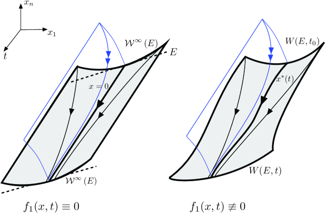
Figure 1: Left: The geometry of the autonomous SSM $\mathcal{W}^{\infty}\left(E\right)$ in the extended phase space of the $(x,t)$ variables. Shown is the primary (smoothest SSM) tangent to the spectral subspace $E$ at the fixed point at $x=0$. Also shown is a fast SSM (blue), defined as the spectral submanifold that is tangent to the direct sum of the eigenspaces outside $E$. Right: The anchor trajectory $x^{*}(t)$ and the time-dependent SSM $W\left(E,t\right)$ in the full, non-autonomous system.

In general, an infinite family, $\mathcal{W}\left(E\right)$, of SSMs exists for system (3) with the same properties, but $\mathcal{W}^{\infty}\left(E\right)$ is the unique smoothest among them: the other manifolds in $\mathcal{W}\left(E\right)$ are no more than $\sigma\left(E\right)$-times differentiable (see Haller et al. [19]). A computational algorithm for $\mathcal{W}^{\infty}\left(E\right)$ was developed by Ponsioen et al. [36], then extended to general, finite-element-grade problems in second-order ODE form by Jain and Haller [24]. The latest version of the latter algorithm with further extensions is available in the open-source MATLAB live script package SSMTool (see Jain et al. [25]).

If the spectrum of $A$ is fully nonresonant, i.e.,

$$\lambda_{j}\neq\sum_{k=1}^{n}m_{k}\lambda_{k},\quad m_{k}\in\mathbb{N},\quad\sum_{k=1}^{n}m_{k}\geq 2,\quad j=1,\ldots,n,$$ (18)

then an invariant manifold family $\mathcal{W}\left(E\right)$ tangent to $E$ at $x=0$ exists for any choice of $E$, whether or not $E$ is of like-mode or mixed mode type. While $\mathcal{W}\left(E\right)$ may contain just a single manifold (e.g., when $E$ is the stable subspace, $E^{s}$ or the unstable subspace, $E^{u}$, defined in (9)), there will be infinitely members in $\mathcal{W}\left(E\right)$ for more general choices of $E$. In the latter case, generic members of $\mathcal{W}\left(E\right)$ are secondary (or fractional) SSMs, which have a finite order of differentiability consistent with their fractional-powered polynomial representations derived explicitly by Haller et al. [19].

Note that the nonresonance conditions (17)-(18) are less restrictive than what is customary in the nonlinear vibrations literature. Indeed, conditions (17)-(18) are only violated if both the real and the complex parts of the eigenvalues satisfy simultaneously exactly the same resonance relationship. Also note that $1:1$ resonances involving eigenvalues with nonzero real parts do not violate (17)-(18). We will, however, only allow a $1\colon 1$ resonance within $E$ to guarantee the normal hyperbolicity of $E$ for the existence of $\mathcal{W}\left(E\right)$. (More specifically, a $1\colon 1$ resonance between the spectrum of $A$ within $E$ and outside $E$ would render our upcoming assumption (19) to fail for any $\rho>1$). If a $1\colon 1$ resonance arises in a given application, one can simply enlarge $E$ to include all resonant modes. This, in turn, removes any issue with the $1\colon 1$ resonance.

We now turn to the existence of non-autonomous SSMs emanating from the uniformly bounded hyperbolic trajectory $x^{*}(t)$, whose existence and approximation were discussed in Theorems 1 and 2. We will focus on slow SSMs (also called pseudo-unstable manifolds), which are continuations of $d$-dimensional, $\rho$-normally attracting (like-mode or mixed-mode) spectral subspaces $E$ of the linearized system (7), i.e., can be written as

$$E=E_{1}\oplus\ldots\oplus E_{k},\qquad\dim E=d\geq 1,\qquad\mathrm{\frac{\mathrm{Re}\text{$\lambda_{k}$}}{\mathrm{Re}\text{$\lambda_{k+1}$}}\leq\frac{1}{\rho}},$$ (19)

for some integer $\rho>1$. Therefore, $E$ is spanned by the $k$ modal subspaces carrying the slowest decaying solution families of system (7), including possibly some families that do not even decay but grow. If such unstable modal subspaces are present in the direct sum (19), then $E$ is a mixed-mode spectral subspace which we seek to continue into a mixed mode non-autonomous SSM in system (1). If, in contrast, only stable modal subspaces are present in the direct sum (19), then $E$ is a like-mode spectral subspace which we seek to continue into a like-mode non-autonomous SSM in system (1).

Note that the third condition in (19) always holds for arbitrary $\rho>1$ if $\mathrm{Re}\lambda_{k}$ and $\mathrm{Re}\lambda_{k+1}$ have different signs. If $\mathrm{Re}\lambda_{k}$ and $\mathrm{Re}\lambda_{k+1}$ have the same sign, then the third condition in (19) holds only if the decay exponents of solutions outside $E$ are at least $\rho$-times stronger than those of solutions inside $E$. This $\rho$ will then determine the maximal smoothness that we can a priori guarantee for the SSM emanating from $E$ without further assumptions. Formal expansions for such SSMs will, however, indicate higher degrees of smoothness under appropriate nonresonance conditions.

The following theorem gives our main result on the existence of non-autonomous SSMs associated with a spectral subspace $E$ satisfying (19). We will use the term locally invariant manifold when referring to a manifold carrying trajectories that can only leave the manifold through its boundary (see, e.g., Fenichel [14]).

Theorem 3.

[Existence of non-autonomous SSMs] Assume that conditions (11) of Theorem 1 are satisfied in a ball $B_{\delta}\subset\mathbb{R}^{n}$ of radius $\delta>0$ around $x=0$. Assume further that $f_{0},f_{1}\in C^{r}(B_{\delta})$ for some $r>1$ and the uniform bound

$$\left|\partial_{x}^{2}f_{1}(x,t)\right|\leq K_{3},\quad x\in B_{\delta},\quad t\in\mathbb{R},$$ (20)

holds for some finite constant $K_{3}>0$. Assume finally that $E$ is a $\rho$-normally hyperbolic spectral subspace with $1<\rho\leq r$ that satisfies the nonresonance conditions

$$\lambda_{j}\neq\sum_{k=1}^{n}m_{k}\lambda_{k},\quad m_{k}\in\mathbb{N},\quad\sum_{k=1}^{n}m_{k}\geq 2,\quad j=1,\ldots,n.$$ (21)

Then:

(i)

There exists a non-autonomous spectral submanifold $W(E,t)\subset B_{\delta}$ of class $C^{\rho}$ that has the same dimension as $E$, contains $x^{*}(t)$ and acts as a locally invariant manifold for system (1).

(ii)

The SSM $W(E,t)$ is as smooth in any parameter as system ((1)).

Proof.

See Appendix B.1. ∎

We sketch the geometry of the non-autonomous SSM, $W(E,t)$, for non-vanishing $f_{1}(x,t)$ in Fig. 1.

Remark 3.

[Uniqueness and smoothness of non-autonomous SSMs] The manifolds discussed in Theorem 3 are generally non-unique. In principle, an argument involving the smoothness of the Lyapunov and dichotomy spectra under generic perturbation (see Son [45]) could be invoked to deduce sharper smoothness results for these manifolds from linearization (see Yomdin [50]). These results, however, require the identification of the full Lyapunov spectrum of the linear part of the non-autonomous linear differential equation (B1) in our Appendix B.1 in order to exclude resonances. This is generally challenging for equations and unrealistic for data sets. As an alternative, Theorem 4 below will provide unique Taylor expansions for $W(E,t)$ under explicitly verifiable nonresonance conditions. These expansions are varied on each persisting non-autonomous SSM up to the degree of smoothness of the SSM. We conjecture that, just as in the time-periodic and time-quasiperiodic case treated by Cabré et al. [5] and Haro and de la Llave [20], a unique member of the $W(E,t)$ family of manifolds will be smoother than all the others. Our Taylor expansion will then approximate those unique, smoothest manifolds at orders higher than the spectral quotient $\Sigma(E)$ defined in Haller and Ponsioen [18]. The remaining manifolds can be constructed via time-dependent versions of the fractional expansions identified in Haller et al. [19].

Remark 4.

[Non-autonomous SSMs without anchor trajectories] For stable hyperbolic fixed points in the $f_{1}(x,t)\equiv 0$ limit, an alternative to the proof in Appendix B.1 for Theorem 3 can also be given. This alternative uses the theory of non-compact normally hyperbolic invariant manifolds (see Eldering [12]) coupled with the “wormhole” construct of Eldering et al. [13] that enables the handling of inflowing-invariant normally attracting invariant manifolds. Following the steps of our proof in Appendix C.2 for the adiabatic case, this alternative proof yields results similar to those in Theorem 3 but does not rely on a persisting anchor trajectory $x^{*}(t)$ near the origin. As a consequence, it can also capture non-autonomous SSMs in weakly damped physical systems for higher forcing levels at which $x^{*}(t)$ is already destroyed. This is because the strength of hyperbolicity of the unforced fixed point at $x=0$ (measured by $\left|\mathrm{Re}\text{$\lambda_{1}$}\right|\ll 1$) is generally much weaker than the strength of hyperbolicity of the unforced SSM, $\mathcal{W}^{\infty}\left(E\right)$, (measured by $\frac{\left|\mathrm{Re}\text{$\lambda_{k+1}$}\right|}{\left|\mathrm{Re}\text{$\lambda_{k}$}\right|}>1$) in weakly damped systems. Such persisting SSMs without a stable hyperbolic anchor trajectory have been well-documented in equation- and data-driven studies of time-periodically forced systems. Those SSMs are signaled by overhangs near resonances in the forced response curves at higher forcing levels (see, e.g., Jain and Haller [24], Cenedese et al. [8]).

As our examples will show, $W(E,t)$ will generally persist even under $f_{1}(x,t)$ perturbations that are significantly larger than those allowed by the rather conservative assumptions of Theorem 1. In addition, $W(E,t)$ will also be smoother than $C^{\rho}$ under additional nonresonance conditions. To this end, we will next derive numerically implementable, recursive approximation formulas that are valid for $W(E,t)$ as long as it persists.

To state these approximations, we first introduce a small perturbation parameter $\epsilon\geq 0$ with which we rescale the non-autonomous term in ((1) as

$$f_{1}(x,t)=\epsilon\tilde{f}_{1}(x,t),$$ (22)

in order to focus on moderate values of $f_{1}(x,t)$. As a consequence of this scaling, the expansion (14) for the anchor trajectory is also rescaled to

$$x_{\epsilon}^{*}(t)=\sum_{\nu=1}^{N}\epsilon^{\nu}\tilde{x}_{\nu}(t)+o\left(\epsilon^{N}\right),$$ (23)

given that the form of the coefficients $x_{\nu}(t)$ in the formulas (15) yields

$$x_{\nu}(t)=\epsilon\tilde{x}_{\nu}(t).$$ (24)

Second, we let $P=[e_{1},\ldots,e_{n}]\in\mathbb{C}^{n}$ contain the complex unit eigenvectors corresponding to the ordered eigenvalues (5) of $A$. Then, under a coordinate change $x\mapsto(u,v)\in\mathbb{C}^{d}\times\mathbb{C}^{n-d}$ defined as

$$\left(\begin{array}[]{c}u\\ v\end{array}\right)=P^{-1}\left(x-x_{\epsilon}^{*}(t)\right),$$ (25)

we obtain a complex system of ODEs

$$\left(\begin{array}[]{c}\dot{u}\\ \dot{v}\end{array}\right) =\left(\begin{array}[]{cc}A^{u}&0\\ 0&A^{v}\end{array}\right)\left(\begin{array}[]{c}u\\ v\end{array}\right)+\hat{f}(u,v,\epsilon;t),$$ (32)

where

$$A^{u}=\left(\begin{array}[]{ccc}\lambda_{1}&0&0\\ 0&\ddots&0\\ 0&0&\lambda_{d}\end{array}\right),\quad A^{v}=\left(\begin{array}[]{ccc}\lambda_{d+1}&0&0\\ 0&\ddots&0\\ 0&0&\lambda_{n}\end{array}\right),$$ (39)

and

$$\hat{f}(u,v,\epsilon;t) =P^{-1}\left[f_{0}\left(x_{\epsilon}^{*}(t)+P\left(\begin{array}[]{c}u\\ v\end{array}\right)\right)+Ax_{\epsilon}^{*}(t)-\dot{x}_{\epsilon}^{*}(t)+\epsilon\tilde{f}_{1}\left(x_{\epsilon}^{*}(t)+P\left(\begin{array}[]{c}u\\ v\end{array}\right),t\right)\right].$$ (44)

In system (32), the fixed point $(u,v)=(0,0)$ corresponds to the anchor trajectory $x_{\epsilon}^{*}(t)$ and the $u$ coordinate space is aligned with the spectral subspace $E$.

Third, using the integer multi-index $\left(\mathbf{k},p\right)\in\mathbb{N}^{d}\times\mathbb{N}$ with $\left|\left(\mathbf{k},p\right)\right|\geq 0$, we define a (now $\epsilon$-dependent) order-$\left|\left(\mathbf{k},p\right)\right|$ approximation to $x_{\epsilon}^{*}(t)$ and the evaluation of $\hat{f}(u,v,\epsilon;t)$ on this approximation as

$$x_{\epsilon}^{*}(t;\mathbf{k},p)=\sum_{\nu=0}^{\left|\mathbf{k}\right|+p-1}\epsilon^{\nu}x_{\nu}(t),\qquad\hat{f}(u,v,\epsilon;t;\mathbf{k},p)=\left(\begin{array}[]{c}\hat{f}^{u}(u,v,\epsilon;t;\mathbf{k},p)\\ \hat{f}^{v}(u,v,\epsilon;t;\mathbf{k},p)\end{array}\right)\in\mathbb{C}^{d}\times\mathbb{C}^{n-d},$$ (45)

respectively, where

$$\hat{f}(u,v,\epsilon;t;\mathbf{k},p) =P^{-1}\left[f_{0}\left(x_{\epsilon}^{*}(t;\mathbf{k},p)+P\left(\begin{array}[]{c}u\\ v\end{array}\right)\right)+Ax_{\epsilon}^{*}(t;\mathbf{k},p)\right.$$ (48)

$$\,\,\,\,\,\,\,\,\,\,\,\,\,\,\,\,\,\,-\left.\dot{x}_{\epsilon}^{*}(t;\mathbf{k},p)+\epsilon\tilde{f}_{1}\left(x_{\epsilon}^{*}(t;\mathbf{k},p)+P\left(\begin{array}[]{c}u\\ v\end{array}\right),t\right)\right].$$ (51)

In short, $x_{\epsilon}^{*}(t;\mathbf{k},p)$ is an approximation of $x^{*}(t)$ in the scaled variable $\epsilon x$ up to order $\left|\mathbf{k}\right|+p-1$. Accordingly, $\hat{f}(u,v,\epsilon;t;\mathbf{k},p)$ is an approximation of $\hat{f}(u,v,\epsilon;t)$ that uses $x_{\epsilon}^{*}(t;\mathbf{k},p)$ instead of $x^{*}(t)$.

Finally, for any multi-index $\mathbf{k}\in\mathbb{N}^{d}$, we define the time-dependent diagonal matrix $G_{\mathbf{k}}(t)\in\mathbb{C}^{\left(n-d\right)\times\left(n-d\right)}$ as

$$\left[G_{\mathbf{k}}(t)\right]_{\ell\ell} :=\left\{\begin{array}[]{ccc}e^{\left[\lambda_{\ell}-\sum_{j=1}^{d}k_{j}\lambda_{j}\right]t},&&\,\,\,\,\mathrm{Re}\left[\lambda_{\ell}-\sum_{j=1}^{d}k_{j}\lambda_{j}\right]<0,\\ \\ 0,&&\mathrm{otherwise},\end{array}\right.\quad t\geq 0,$$ (55)

(56)

$$\left[G_{\mathbf{k}}(t)\right]_{\ell\ell} :=\left\{\begin{array}[]{ccc}-e^{\left[\lambda_{\ell}-\sum_{j=1}^{d}k_{j}\lambda_{j}\right]t},&&\mathrm{Re}\left[\lambda_{\ell}-\sum_{j=1}^{d}k_{j}\lambda_{j}\right]>0,\\ \\ 0,&&\mathrm{otherwise},\end{array}\right.\quad t<0,$$ (60)

for $\ell=d+1,\ldots,n.$ Using these quantities, we can state the following results.

Theorem 4.

[Computation of non-autonomous SSMs and their reduced dynamics] Assume that after the rescaling (22), an $\epsilon$-dependent SSM, $W_{\epsilon}(E,t)$, of the type described in Theorem 3 exists in the coordinates $(u,v)$ for system (32) for all $\epsilon\in\left[0,\epsilon^{*}\right]$. Assume further that $W_{\epsilon}(E,t)$ is $N$-times continuously differentiable for any fixed $t$ and the nonresonance conditions

$$\mathrm{Re}\,\lambda_{j}\neq\sum_{\lambda_{k}\in\mathrm{spect}\left(A|_{E}\right)}m_{k}\mathrm{Re}\,\lambda_{k},\qquad\lambda_{j}\in\mathrm{spect}\left(A\right)-\mathrm{spect}\left(A|_{E}\right),$$ (61)

hold for all $j=k+1,\ldots,n$ and for all $m_{k}\in\mathbb{N}$ with

$$1\leq\sum_{k=1}^{n}m_{k}\leq N.$$ (62)

.

Then, for all $\epsilon\in\left[0,\epsilon^{*}\right]$:

(i)

The SSM $W_{\epsilon}(E,t)$ admits a formal asymptotic expansion

$$W_{\epsilon}\left(E,t\right)=\left\{\left(u,v\right)\in U\subset\mathbb{R}^{n}:\,v=h_{\epsilon}(u,t)=\sum_{\left|\left(\mathbf{k},p\right)\right|\geq 1}^{N}h^{\mathbf{k}p}(t)u^{\mathbf{k}}\epsilon^{p}+o\left(\left|u\right|^{q}\epsilon^{N-q}\right)\right\}.$$ (63)

The uniformly bounded $h^{\mathbf{k}p}(t)$ coefficients in this expansion can be computed recursively from their initial conditions

$$h^{\mathbf{0}p}(t)\equiv 0,\quad t\in\mathbb{R},\quad p\in\mathbb{N};\qquad h^{\mathbf{k}0}(t)\equiv-A_{\mathbf{k}}^{-1}M^{\mathbf{k}0}(h^{\mathbf{j}0}),\quad\left|\mathbf{j}\right|<\left|\mathbf{k}\right|;\quad h^{\mathbf{0}0}=0,$$ (64)

via the formula

$$h^{\mathbf{k}p}(t)=\int_{-\infty}^{\infty}G_{\mathbf{k}}(t-s)M^{\mathbf{k}p}(s,h^{\mathbf{j}m}(s))\,ds,\quad\left|(\mathbf{j},m)\right|<\left|(\mathbf{k},p)\right|,\quad t\in\mathbb{R},$$ (65)

where the functions $M^{\mathbf{k}p}$ are defined as

$$M^{\mathbf{k}p}(t,h^{\mathbf{j}m})=\frac{\partial^{\left|\left(\mathbf{k},p\right)\right|}}{\partial u_{1}^{k_{1}}\ldots\partial u_{d}^{k_{d}}\partial\epsilon^{p}}\left[\hat{f}^{v}\left(u,\sum_{\left|\left(\mathbf{j},m\right)\right|\geq 1}^{\left|\left(\mathbf{k},p\right)\right|-1}h^{\mathbf{j}m}(t)u^{\mathbf{j}}\epsilon^{m},\epsilon;t;\mathbf{k},p\right)\right.$$

$$-\left.\left.\sum_{\left|\left(\mathbf{j},m\right)\right|\geq 1}^{\left|\left(\mathbf{k},p\right)\right|-1}\epsilon^{p}\left(\begin{array}[]{ccc}h_{1}^{\mathbf{j}m}(t)\frac{j_{1}u^{\mathbf{j}}}{u_{1}}&\cdots&h_{1}^{\mathbf{j}m}(t)\frac{j_{d}u^{\mathbf{j}}}{u_{d}}\\ \vdots&\ddots&\vdots\\ h_{n-d}^{\mathbf{j}m}(t)\frac{j_{1}u^{\mathbf{j}}}{u_{1}}&\cdots&h_{n-d}^{\mathbf{j}m}(t)\frac{j_{d}u^{\mathbf{j}}}{u_{d}}\end{array}\right)\hat{f}^{u}\left(u,\sum_{\left|\left(\mathbf{j},m\right)\right|\geq 1}^{\left|\left(\mathbf{k},p\right)\right|-1}h^{\mathbf{j}m}(t)u^{\mathbf{j}}\epsilon^{m},\epsilon;t;\mathbf{k},p\right)\right]\right|_{u=0,\,\epsilon=0}.$$ (66)

(ii)

The reduced dynamics on $W_{\epsilon}\left(E,t\right)$ is obtained by restricting the $u$-component of system (32) to $W_{\epsilon}\left(E,t\right)$, which yields

$$\dot{u} =A^{u}u$$ (67)

$$+Q_{u}\left[f_{0}\left(x_{\epsilon}^{*}(t)+P\left(\begin{array}[]{c}u\\ h_{\epsilon}(u,t)\end{array}\right)\right)+\epsilon\tilde{f}_{1}\left(x_{\epsilon}^{*}(t)+P\left(\begin{array}[]{c}u\\ h_{\epsilon}(u,t)\end{array}\right),t\right)+Ax_{\epsilon}^{*}(t)-\dot{x}_{\epsilon}^{*}(t)\right].$$ (72)

Here $Q_{u}\in\mathbb{C}^{d\times n}$ is a matrix whose $j^{th}$ row is $\hat{e}_{j}/\left(\hat{e}_{j}\cdot e_{j}\right)$ for $j=1,\ldots d$, where $\hat{e}_{j}$ is the $j^{th}$ unit left eigenvector of $P$ corresponding to its unit right eigenvector $e_{j}$. Equivalently, $Q_{u}$ is composed of the first $d$ rows of $P^{-1}$.

(iii)

Let $\left(\xi,\eta\right)^{\mathrm{T}}=P^{-1}x$ denote coordinates aligned with the subspace $E$ and the direct sum of the remaining eigenspaces, respectively, emanating from the original $x=0$ fixed point of system (1) for $\epsilon=0.$ In these coordinates, the reduced dynamics (67) becomes

$$\dot{\xi} =A^{u}\xi$$ (73)

$$+Q_{u}\left[f_{0}\left(x_{\epsilon}^{*}(t)+P\left(\begin{array}[]{c}\xi-Q_{u}x_{\epsilon}^{*}(t)\\ h_{\epsilon}(\xi-Q_{u}x_{\epsilon}^{*}(t),t)\end{array}\right)\right)+\epsilon\tilde{f}_{1}\left(x_{\epsilon}^{*}(t)+P\left(\begin{array}[]{c}\xi-Q_{u}x_{\epsilon}^{*}(t)\\ h_{\epsilon}(\xi-Q_{u}x_{\epsilon}^{*}(t),t)\end{array}\right),t\right)\right].$$ (78)

Proof.

See Appendix B.2. ∎

Remark 5.

[Related results] Pötzsche and Rassmussen [41] derive Taylor approximations for a broad class of invariant manifolds emanating from fixed points of non-autonomous ODE. Due to the generality of that setting, the resulting formulas are less explicit than ours, assume global boundedness on the nonlinear terms, and also assume that the origin remains a fixed point for all times (and hence disallow additive external forcing). Nevertheless, under further assumptions and appropriate reformulations, those formulas should ultimately yield results equivalent to ours when applied to SSMs. Although it does not directly overlap with our results here, we also mention related work by Pötzsche and Rassmussen [40] on the computation of classic and strong stable/unstable manifolds, as well as center-stable/unstable manifolds, for non-autonomous difference equations.

Remark 6.

[Extension to discontinuous forcing] The derivatives in the definition of (66) can be evaluated using the same higher-order chain-rule formula of Constantine and Savits [10] that we applied in the proof of Theorem 2. Using these formulas reveal that $h^{\mathbf{k}p}(t)$ can be formally computed as long as $f_{1}$ and its $x$-derivatives at $x=0$ remain uniformly bounded in $t$. Therefore, the formal expansion we have derived for the SSM $W_{\epsilon}\left(E,t\right)$ is valid for small enough $\epsilon$ even if $f_{1}$ is discontinuous in the time $t$. We illustrate the continued accuracy of these expansions for discontinuous forcing on an example in Section 4.1.1.

Remark 7.

[Relation to the case of periodic or quasi-periodic forcing] The recursively defined coefficient vectors $M^{\mathbf{k}p}(s,h^{\mathbf{j}m}(s))$ defined in eq. (66) are explicitly time dependent but otherwise satisfy the same formulas as the terms on the right-hand side of the invariance equations arising from autonomous SSM calculations. Consequently, the recursive formulas originally implemented in SSMTool by Jain et al. [25] for autonomous SSM calculations apply here without modification. The difference is that those autonomous $M^{\mathbf{k}}$ coefficients are used in solving linear algebraic systems of equations for $h^{\mathbf{k}}$, as opposed to the non-autonomous $M^{\mathbf{k}p}$ coefficients are used in linear ODEs for $h^{\mathbf{k}p}(t)$.

Remark 8.

[Accuracy of asymptotic SSM formulas] The accuracy of the reduced-order dynamics (67) increases with increasing $\left|(\mathbf{k},p)\right|$. There is no general convergence result under $N\to\infty$ in the reduced dynamics (67), but such convergence is known if $f(x,t)$ is analytic and has periodic or quasi-periodic time dependence Cabré et al. [5], Haro and de la Llave [20]). For those types of time dependencies, the $\mathcal{O}\left(\epsilon\right)$ term in the reduced dynamics (67) is the same as that used for time-periodic and time-quasiperiodic SSMs in earlier publications (see, e.g., Breunung and Haller [4], Cenedese et al. [9]).

By formula (73), in the $\xi$ coordinate aligned with $E$ and emanating from $x=0$, the reduced dynamics up to first order in $\epsilon$ is of the form

$$\dot{\xi} =A^{u}\xi+Q_{u}f_{0}\left(P\left(\begin{array}[]{c}\xi\\ h_{0}(\xi)\end{array}\right)\right)$$ (81)

$$+\epsilon Q_{u}\left[Df_{0}\left(P\left(\begin{array}[]{c}\xi\\ h_{0}(\xi)\end{array}\right)\right)\left(\int_{-\infty}^{t}e^{A\left(t-\tau\right)}\tilde{f}_{1}(0,\tau)\,d\tau-P\left(\begin{array}[]{c}Q_{u}\int_{-\infty}^{t}e^{A\left(t-\tau\right)}\tilde{f}_{1}(0,\tau)\,d\tau\\ \partial_{\epsilon}h_{\epsilon}(\xi,t)|_{\epsilon=0}\end{array}\right)\right)\right]$$ (86)

$$+\epsilon Q_{u}\tilde{f}_{1}\left(P\left(\begin{array}[]{c}\xi\\ h_{0}(\xi)\end{array}\right),t\right)$$ (89)

$$+o\left(\epsilon\right),$$ (90)

where we used formulas (16) and (24) in evaluating $\tilde{x}_{1}(t)$, the first coefficient in the expansion of $x_{\epsilon}^{*}(t)$ in eq. (23).

In prior treatments of time-periodically and time-quasi-periodically forced SSMs, the second line on the right-hand side of eq. (90) has been justifiably dropped in leading-order approximations, because the factor $Df_{0}\left(P\left(\begin{array}[]{c}\xi\\ h_{0}(\xi)\end{array}\right)\right)$ is small close to the origin (see, e.g., Breunung and Haller [4], Ponsioen et al. [38], Jain and Haller [24], Cenedese et al. [8]). In that case, the leading-order correction to the unforced reduced dynamics is simply the third line in (90), which is just the projection of the restriction of the forcing term to the autonomous SSM onto the spectral subspace $E$. If, in addition, the forcing term only depends on time (i.e., $\partial_{x}\tilde{f}_{1}\equiv 0$), as is often the case in structural vibrations, then a leading-order approximation for small-amplitude motions on the SSM $W_{\epsilon}\left(E,t\right)$ becomes

$$\dot{\xi} =A^{u}\xi+Q_{u}f_{0}\left(P\left(\begin{array}[]{c}\xi\\ h_{0}(\xi)\end{array}\right)\right)+\epsilon Q_{u}\tilde{f}_{1}\left(t\right)+\mathcal{O}\left(\epsilon\left|\xi\right|,\epsilon^{2}\right).$$ (93)

This level of approximation of the reduced dynamics was shown to be accurate for small $\epsilon$ and $\left|\xi\right|$ for periodic and quasi-periodic forcing by the references cited above. Equation (93) now establishes the same approximation formula for general, $x$-independent forcing $f_{1}(t)=\epsilon\tilde{f}_{1}\left(t\right)$ for trajectories that stay close to the origin. Under general forcing, however, trajectories may well stray away from the origin, given that $W_{\epsilon}\left(E,t\right)$ itself will generally move substantially away from the origin. In that case, the next level of approximation obtained from eq. (90) is

$$\dot{\xi} =A^{u}\xi+Q_{u}f_{0}\left(P\left(\begin{array}[]{c}\xi\\ h_{0}(\xi)\end{array}\right)\right)$$ (96)

$$+\epsilon Q_{u}\left[Df_{0}\left(P\left(\begin{array}[]{c}\xi\\ 0\end{array}\right)\right)\left(\int_{-\infty}^{t}e^{A\left(t-\tau\right)}\tilde{f}_{1}(0,\tau)\,d\tau-P\left(\begin{array}[]{c}Q_{u}\int_{-\infty}^{t}e^{A\left(t-\tau\right)}\tilde{f}_{1}(0,\tau)\,d\tau\\ \partial_{\epsilon}h_{\epsilon}(\xi,t)|_{\epsilon=0}\end{array}\right)\right)\right]$$ (101)

$$+\epsilon Q_{u}\tilde{f}_{1}\left(P\left(\begin{array}[]{c}\xi\\ 0\end{array}\right),t\right)$$ (104)

$$+\mathcal{O}\left(\epsilon\left|\xi\right|^{2},\epsilon^{2}\right).$$ (105)

Higher-order approximation can be systematically developed by Taylor-expanding the reduced dynamics (73) in $\epsilon$ and utilizing the terms from the expansions for $x_{\epsilon}^{*}(t)$ and $W_{\epsilon}\left(E,t\right)$ using Theorems 2 and 4.

Alternative parametrizations of $W_{\epsilon}\left(E,t\right)$ beyond the graph-style parametrization worked out here in detail are also possible (see Haller and Ponsioen [18], Haro et al. [21], Vizzaccaro et al. [48]). One option is the normal-form style parameterization which simultaneously brings the reduced dynamics on $W_{\epsilon}\left(E,t\right)$ to normal form. Normal form transformations can also be applied separately once $W_{\epsilon}\left(E,t\right)$ is located (see, e.g., Cenedese et al. [8]).

3 Adiabatic SSMs

3.1 Setup

We now consider slowly varying non-autonomous dynamical systems of the form

$$\dot{x}=f(x,\epsilon t),\quad x\in\mathbb{R}^{n},\quad f\in C^{r},\quad 0\leq\epsilon\ll 1,$$ (106)

for some integer $r\geq 1$. We obtain such a system, for instance, when we replace the forcing function $f_{1}(x,t)$ in system (1) with its slowly varying counterpart, $f_{1}(x,\epsilon t)$, in which case we have $f(x,\epsilon t)=Ax+f_{0}(x)+f_{1}(x,\epsilon t).$ The form in (106) is, however, more general than this specific example.

Introducing the slow variable $\alpha=\epsilon t$, we rewrite system (106) as

$$\dot{x} =f(x,\alpha),$$ (107)

$$\dot{\alpha} =\epsilon.$$

For $\epsilon=0$, we assume that the $x$-component of system (107) has an $\alpha$-dependent, uniformly bounded and uniformly hyperbolic fixed point $x_{0}(\alpha)$, i.e., with the notation

$$A(\alpha)=D_{x}f(x_{0}(\alpha),\alpha)\in\mathbb{R}^{n\times n},$$ (108)

we have

$$f(x_{0}(\alpha),\alpha)=0,\quad\left|\mathrm{Re}\left[\mathrm{spect}\left(A(\alpha)\right)\right]\right|\geq K>0,\quad\alpha\in\mathbb{R},$$ (109)

for some constant $K>0$. We further assume that $x_{0}(\alpha)$ is a class $C^{r}$ function of $\alpha$, in which case, by the first equation in (109), we have

$$\frac{d^{p}}{d\alpha^{p}}f(x_{0}(\alpha),\alpha)\equiv 0,\quad 0\leq p\leq r,\quad\alpha\in\mathbb{R}.$$ (110)

By the hyperbolicity assumption (109), we can order the spectrum of $A(\alpha)$ as

$$\mathrm{spect}A(\alpha)=\left\{\lambda_{1}(\alpha),\ldots,\lambda_{n}(\alpha)\right\},$$

so that it satisfies

$$\mathrm{Re}\,\lambda_{n}(\alpha)\leq\ldots\leq\mathrm{Re}\,\lambda_{j}(\alpha)\leq-K<0<K\leq\mathrm{Re}\,\lambda_{j-1}(\alpha)\leq\ldots\leq\mathrm{Re}\,\lambda_{1}(\alpha),\qquad\alpha\in\mathbb{R},$$ (111)

for some $j\geq 1$. Conditions (109) imply that for $\epsilon=0$, the slow-fast system (107) has a one-dimensional, normally attracting, non-compact (but uniformly bounded) invariant manifold of the form

$$\mathcal{L}_{0}=\left\{(x,\alpha)\in\mathbb{R}^{n}\times\mathbb{R}\colon\,\,\,\,\,x=x_{0}(\alpha)\right\}.$$ (112)

The manifold $\mathcal{L}_{0}$ is composed of fixed points of system (107) for $\epsilon=0$ and hence is called a critical manifold in the language of geometric singular perturbation theory (Fenichel [15]).

3.2 Existence and computation of an adiabatic anchor trajectory

As in the non-autonomous case treated in Section 2, we first discuss the continued existence of an anchor trajectory that acts as a continuation of the critical manifold $\mathcal{L}_{0}$.

Theorem 5.

[Existence and computation of anchor trajectory for adiabatic SSMs] For $\epsilon>0$ small enough, there exists a unique, attracting, one-dimensional slow manifold $\mathcal{L}_{\epsilon}$, composed of a slow trajectory $x_{\epsilon}(\alpha)$ that is uniformly bounded in $\alpha\in\mathbb{R}$. The trajectory $x_{\epsilon}(\alpha)$ is $\mathcal{O}\left(\epsilon\right)$ $C^{1}$-close and $C^{r}$ diffeomorphic to the critical manifold $\mathcal{L}_{0}$ defined in (112). Finally, for any nonnegative integer $N\leq r$, $x_{\epsilon}(\alpha)$ can be approximated as

$$\mathcal{L}_{\epsilon}=\left\{(x,\alpha)\in\mathbb{R}^{n}\times\mathbb{R}\colon\,\,\,\,\,x=x_{\epsilon}(\alpha)=\sum_{\nu=0}^{N}\epsilon^{\nu}x_{\nu}(\alpha)+o\left(\epsilon^{N}\right)\right\},$$ (113)

with the recursively defined coefficients

$$x_{\nu}(\alpha)=A^{-1}(\alpha)\left[x_{\nu-1}^{\prime}(\alpha)-\sum_{1<\left|\mathbf{\boldsymbol{\gamma}}\right|\leq\nu}\frac{\partial^{\left|\mathbf{\mathbf{\boldsymbol{\gamma}}}\right|}f\left(x_{0}(\alpha),\alpha\right)}{\partial x_{1}^{\gamma_{1}}\ldots\partial x_{n}^{\gamma_{n}}}\sum_{s=1}^{\nu}\sum_{p_{s}\left(\nu,\mathbf{\boldsymbol{\gamma}}\right)}\prod_{j=1}^{s}\frac{\prod_{i=1}^{n}\left[x_{\ell_{j}}^{i}(\alpha)\right]^{k_{ji}}}{\prod_{i=1}^{n}k_{ji}!}\right],\quad\nu\geq 1,$$ (114)

where the index set $p_{s}\left(\nu,\mathbf{\mathbf{\boldsymbol{\gamma}}}\right)$ is defined as

$$p_{s}\left(\nu,\mathbf{\mathbf{\boldsymbol{\gamma}}}\right)=\left\{\left(\mathbf{k}_{1},\ldots,\mathbf{k}_{s},\ell_{1},\ldots,\ell_{s}\right):\mathbf{k}_{i}\in\mathbb{N}^{n}-\left\{\mathbf{0}\right\},\ell_{i}\in\mathbb{N},0<\ell_{1}<\cdots<\ell_{s},\sum_{i=1}^{s}\mathbf{k}_{i}=\mathbf{\boldsymbol{\gamma}},\sum_{i=1}^{s}\left|\mathbf{k}_{i}\right|\ell_{i}=\nu\right\}.$$

Proof.

See Appendix C.1. ∎

Specifically, for $N=2$, formula (114) gives an approximation for the slow anchor trajectory $x_{\epsilon}(\alpha)$ in the form

$$x_{\epsilon}(\alpha) =x_{0}(\alpha)+\epsilon x_{1}(\alpha)+\epsilon^{2}x_{2}(\alpha)+o\left(\epsilon^{2}\right),$$

$$x_{1}(\alpha) =\left[D_{x}f(x_{0}(\alpha),\alpha)\right]^{-1}x_{0}^{\prime}(\alpha),$$

$$x_{2}(\alpha) =\left[D_{x}f(x_{0}(\alpha),\alpha)\right]^{-1}\left[x_{1}^{\prime}(\alpha)-\frac{1}{2}D_{x}^{2}f\left(x_{0}(\alpha),\alpha\right)\otimes x_{1}(\alpha)\otimes x_{1}(\alpha)\right].$$ (115)

3.3 Existence and computation of an adiabatic SSM

We seek to construct an adiabatic SSM anchored along the slow invariant manifold $\mathcal{L}_{\epsilon}$ that is spanned by $x_{\epsilon}(\alpha)$ for small $\epsilon>0$. To this end, we assume that the first $k$ eigenvalues $\lambda_{1}(\alpha),\ldots,\lambda_{k}(\alpha)$ in the list (111) have negative real parts and there is a nonzero spectral gap between $\mathrm{Re}\,\lambda_{k}(\alpha)$ and $\mathrm{Re}\,\lambda_{k+1}(\alpha)$:

$$\mathrm{Re}\,\lambda_{n}(\alpha)\leq\ldots\leq\mathrm{Re}\,\lambda_{k+1}(\alpha)<\mathrm{Re}\,\lambda_{k}(\alpha)\leq\ldots\leq\mathrm{Re}\,\lambda_{1}(\alpha)<0,\qquad\alpha\in\mathbb{R}.$$ (116)

We also assume that the real spectral subspace $E(\alpha)$ formed by the corresponding first $k$ eigenvalues varies smoothly in $\alpha$ and hence has a constant dimension

$$d=\dim E(\alpha),\quad\alpha\in\mathbb{R}.$$

We then define the integer part $\rho$ of the spectral gap associated with $E(\alpha)$ as

$$\rho=\min_{\alpha\in\mathbb{R}}\mathrm{Int}\left[\frac{\mathrm{Re}\,\lambda_{k+1}(\alpha)}{\mathrm{Re}\,\lambda_{k}(\alpha)}\right]\in\mathbb{N}^{+}.$$ (117)

Note that $\rho\geq 1$ holds by assumption (116), with $\rho$ measuring the minimum of how many times the attraction rates toward $E(\alpha)$ overpower the contraction rates within $E(\alpha)$.

For $\epsilon=0$ and for each $\alpha\in\mathbb{R}$, system (107) has an SSM $W_{0}\left(E(\alpha)\right)$ tangent to $E(\alpha)$ at $x_{0}(\alpha)$ (see Haller and Ponsioen [18]). As a consequence,

$$\mathcal{M}_{0}=\underset{\alpha\in\mathbb{R}}{\cup}W_{0}\left(E(\alpha)\right)$$

is a $(d+1)$-dimensional, $\rho$-normally attracting invariant manifold for system (107) for $\epsilon=0$ in the sense of Fenichel [14] and Eldering et al. [13]. More specifically, $\mathcal{M}_{0}$ is a $\rho$-normally attracting, non-compact, inflowing-invariant manifold with a boundary, as shown in Fig. 2 for $\epsilon=0$ .

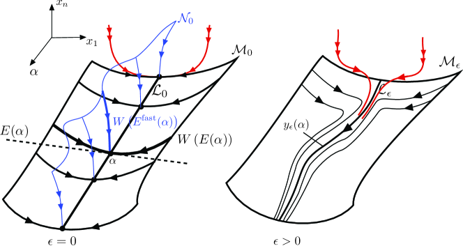
Figure 2: Left: The geometry of the critical manifold $\mathcal{L}_{0}$ (spanned by the anchor trajectory $x_{0}(\alpha)$), the attracting invariant manifold $\mathcal{M}_{0}$, and the fast stable manifold $\mathcal{N}_{0}$ (blue) of $\mathcal{L}_{0}$. Two trajectories off these manifolds are shown in red. Right: the persistent slow manifold $\mathcal{L}_{\epsilon}$ (spanned by $x_{\epsilon}(\alpha)$) and and the adiabatic SSM $\mathcal{M}_{\epsilon}$ for small enough $\epsilon>0$.

We have the following main results on the persistence of the manifold $\mathcal{M}_{0}$ in the form of an adiabatic SSM for small enough $\epsilon$.

Theorem 6.

[Existence of adiabatic SSMs] Assume that $x_{0}(\alpha)$ and $f(x,\alpha)$ have $r$ continuous derivatives that are uniformly bounded in $\alpha\in\mathbb{R}$ in a small, closed neighborhood of $\mathcal{M}_{0}.$ Let $m=\min\left(r,\rho\right).$ Then, for $\epsilon>0$ small enough, there exists a persistent invariant manifold (adiabatic SSM anchored along $\mathcal{L}_{\epsilon}$), denoted $\mathcal{M}_{\epsilon}$, that is $C^{m}$ diffeomorphic to $\mathcal{M}_{0}$, has $m$ uniformly bounded derivatives and is $\mathcal{O}\left(\varepsilon\right)$ $C^{1}$ -close to $\mathcal{M}_{0}$. Furthermore, $\mathcal{L}_{\epsilon}\subset\mathcal{M}_{\epsilon}$ holds.

Proof.

See Appendix B.2. ∎

We show the geometry of the adiabatic SSM, $\mathcal{M}_{\epsilon}$, in Fig. 2 for $\epsilon>0$ .

Remark 9.

[Applicability to mixed-mode adiabatic SSMs] For the purposes of constructing $\mathcal{M}_{\epsilon}$, we had to assume in eq. (116) that the spectrum of $A(\alpha)$ lies in the negative complex half plane, i.e., $E(\alpha)$ contains only stable directions. In the terminology of Haller et al. [19], this means that $W\left(E(\alpha)\right)$ has to be a like-mode SSM for all values of $\alpha$ for Theorem 6 to apply. This enables us to select an inflowing-invariant, normally attracting manifold $\mathcal{\tilde{M}}_{0}$ in our proof to which the wormhole construct in Proposition B1 of Eldering et al. [13] is applicable. There is every indication that $\mathcal{M}_{\epsilon}$ also exists under the weaker assumption (109), which only requires $A(\alpha)$ to have no eigenvalues on the imaginary axes, and hence allows $W\left(E(\alpha)\right)$ to be a mixed-mode SSM that contains both stable and unstable directions. In this case however, an $\mathcal{\tilde{M}}_{0}$ with an inflowing or overflowing boundary cannot be chosen and hence Proposition B1 of Eldering et al. [13] would need a technical extension that we will not pursue here, although it appears doable. We simply note that the asymptotic formulas we will derive for $\mathcal{M}_{\epsilon}$ are formally valid under the weaker assumption (109) as well (i.e., for mixed-mode $W\left(E(\alpha)\right)$), as long as $E(\alpha)$ is normally hyperbolic, i.e., attracts solutions at a rate that is uniformly stronger than the contraction rates inside $E(\alpha)$. We will evaluate and confirm these formulas in an example with a mixed mode adiabatic SSMs in Section 4.2.2.

As in the general non-autonomous case treated in Section 2, the adiabatic $\mathcal{M}_{\epsilon}$ will generally persist for larger values of $\epsilon$ and will also be smoother than $C^{m}$ under additional nonresonance conditions. In the following, we will provide a numerically implementable recursive scheme for computing $\mathcal{M}_{\epsilon}$, assuming that it exists and is smooth enough.

To state these recursive approximation results, we first introduce the new coordinates

$$\left(\begin{array}[]{c}u\\ v\end{array}\right)=P^{-1}\left(\alpha\right)\left(x-x_{\epsilon}(\alpha)\right),$$ (118)

where $P(\alpha)\in\mathbb{C}^{n}$ diagonalizes the matrix $A(\alpha)$. The coordinates $\left(u,v\right)\in\mathbb{C}^{d}\times\mathbb{C}^{n-d}$ align with the $d$-dimensional stable spectral subspace family $E(\alpha)$ and with the direct sum of the remaining eigenspaces of $A(\alpha)$, respectively. In these new coordinates, system (107) becomes

$$\left(\begin{array}[]{c}\dot{u}\\ \dot{v}\end{array}\right) =\left(\begin{array}[]{cc}A^{u}\left(\alpha\right)&0\\ 0&A^{v}\left(\alpha\right)\end{array}\right)\left(\begin{array}[]{c}u\\ v\end{array}\right)+\hat{f}(u,v,\epsilon;\alpha),$$ (125)

$$\dot{\alpha} =\epsilon,$$

where

$$A^{u}\left(\alpha\right)=\left(\begin{array}[]{ccc}\lambda_{1}\left(\alpha\right)&0&0\\ 0&\ddots&0\\ 0&0&\lambda_{d}\left(\alpha\right)\end{array}\right),\quad A^{v}\left(\alpha\right)=\left(\begin{array}[]{ccc}\lambda_{d+1}\left(\alpha\right)&0&0\\ 0&\ddots&0\\ 0&0&\lambda_{n}\left(\alpha\right)\end{array}\right),$$ (132)

and

$$\hat{f}(u,v,\epsilon;\alpha)=P^{-1}\left(\alpha\right)\left[f\left(x_{\epsilon}(\alpha)+P\left(\alpha\right)\left(\begin{array}[]{c}u\\ v\end{array}\right),\alpha\right)-A\left(\alpha\right)P\left(\alpha\right)\left(\begin{array}[]{c}u\\ v\end{array}\right)-\epsilon x_{\epsilon}^{\prime}(\alpha)-\epsilon P^{\prime}\left(\alpha\right)\left(\begin{array}[]{c}u\\ v\end{array}\right)\right].$$ (133)

By existing SSM theory, any $\alpha=const.$ slice of $\mathcal{M}_{0}$ can be written in the form of a Taylor expansion in $u$ with coefficients depending smoothly on $\alpha$. Therefore, the whole of $\mathcal{M}_{0}$ can be written as

$$\mathcal{M}_{0}=\cup_{\alpha\in\mathbb{R}}W_{0}\left(E(\alpha)\right)=\left\{\left(u,v,\alpha\right)\in U\subset\mathbb{R}^{n}:\,v=h_{0}(u,\alpha)=\sum_{\left|\mathbf{k}\right|\geq 2}^{r}h^{\mathbf{k}}(\alpha)u^{\mathbf{k}}+o\left(\left|u\right|^{r}\right)\right\}.$$ (134)

We can now state the following results on the computation of the adiabatic SSM, $\mathcal{M}_{\epsilon}$, for $\epsilon\geq 0$.

Theorem 7.

[Computation of adiabatic SSMs] Assume that an $\epsilon$-dependent adiabatic SSM, $\mathcal{M}_{\epsilon}$, of the type described in Theorem 6 exists in the transformed system (125) for all $\epsilon\in\left[0,\epsilon^{*}\right]$ . Assume further that $\mathcal{M}_{\epsilon}$ is $N$-times continuously differentiable and the nonresonance conditions

$$\lambda_{j}(\alpha)\neq\sum_{\lambda_{k}(\alpha)\in\mathrm{spect}\left(A(\alpha)|_{E(\alpha)}\right)}m_{k}\lambda_{k}(\alpha),\qquad\lambda_{j}(\alpha)\in\mathrm{spect}\left(A(\alpha)\right)-\mathrm{spect}\left(A(\alpha)|_{E}(\alpha)\right),$$ (135)

hold for all $j=k+1,\ldots,n$ and for all $m_{k}\in\mathbb{N}$ with

$$1\leq\sum_{k=1}^{n}m_{k}\leq N.$$ (136)

Then, for all $\epsilon\in\left[0,\epsilon^{*}\right]$ :

(i)

The adiabatic SSM, $\mathcal{M}_{\epsilon}$, admits a formal asymptotic expansion

$$\mathcal{M}_{\epsilon}=\left\{\left(u,v,\alpha\right)\in U\subset\mathbb{R}^{n}:\,v=h_{\epsilon}(u,\alpha)=\sum_{\left|\left(\mathbf{k},p\right)\right|\geq 1}^{N}h^{\mathbf{k}p}(\alpha)u^{\mathbf{k}}\epsilon^{p}+o\left(\left|u\right|^{q}\epsilon^{N-q}\right)\right\}.$$ (137)

The functions $h^{\mathbf{k}p}(\alpha)$ are uniformly bounded in $\alpha\in\mathbb{R}$ for all $\left(\mathbf{k},p\right)$ and can be computed recursively from their initial conditions

$$h^{\mathbf{0}p}(\alpha) \equiv 0,\quad p\geq 0;\quad h^{\mathbf{k}0}(\alpha)\equiv h^{\mathbf{k}}(\alpha),\quad\mathbf{k}\in\mathbb{N}^{d};$$ (138)

$$h^{\mathbf{k}0}(\alpha) \equiv h^{\mathbf{k}0}(\alpha)\equiv h^{\mathbf{k}}(\alpha)=0,\quad\left|\mathbf{k}\right|=1;\quad h^{\mathbf{k}(-1)}(\alpha):=0,$$

via the formula

$$h^{\mathbf{k}p}(\alpha)=A_{\mathbf{k}}^{-1}(\alpha)\left[\left[h^{\mathbf{k}(p-1)}\right]^{\prime}(\alpha)-M^{\mathbf{k}p}(\alpha,h^{\mathbf{j}m})\right],\quad\left|(\mathbf{j},m)\right|<\left|(\mathbf{k},p)\right|,$$ (139)

where

$$A_{\mathbf{k}}(\alpha)=\mathrm{diag}\left[\lambda_{\ell}(\alpha)-\sum_{j=1}^{d}k_{j}\lambda_{j}(\alpha)\right]_{\ell=d+1}^{n}\in\mathbb{C}^{\left(n-d\right)\times\left(n-d\right)},$$

$$M^{\mathbf{k}p}(\alpha,h^{\mathbf{j}m})=\frac{\partial^{\left|\left(\mathbf{k},p\right)\right|}}{\partial u_{1}^{k_{1}}\ldots\partial u_{d}^{k_{d}}\partial\epsilon^{p}}\left[\hat{f}^{v}\left(u,\sum_{\left|\left(\mathbf{j},m\right)\right|\geq 1}^{\left|\left(\mathbf{k},p\right)\right|-1}h^{\mathbf{j}m}(\alpha)u^{\mathbf{j}}\epsilon^{m},\epsilon;\alpha;\mathbf{k},p\right)\right.$$

$$-\left.\left.\sum_{\left|\left(\mathbf{j},m\right)\right|\geq 1}^{\left|\left(\mathbf{k},p\right)\right|-1}\epsilon^{p}\left(\begin{array}[]{ccc}h_{1}^{\mathbf{j}m}(\alpha)\frac{j_{1}u^{\mathbf{j}}}{u_{1}}&\cdots&h_{1}^{\mathbf{j}m}(\alpha)\frac{j_{d}u^{\mathbf{j}}}{u_{d}}\\ \vdots&\ddots&\vdots\\ h_{n-d}^{\mathbf{j}m}(\alpha)\frac{j_{1}u^{\mathbf{j}}}{u_{1}}&\cdots&h_{n-d}^{\mathbf{j}m}(\alpha)\frac{j_{d}u^{\mathbf{j}}}{u_{d}}\end{array}\right)\hat{f}^{u}\left(u,\sum_{\left|\left(\mathbf{j},m\right)\right|\geq 1}^{\left|\left(\mathbf{k},p\right)\right|-1}h^{\mathbf{j}m}(\alpha)u^{\mathbf{j}}\epsilon^{m},\epsilon;\alpha;\mathbf{k},p\right)\right]\right|_{u=0,\,\epsilon=0}.$$ (140)

Specifically, for $\epsilon=0$, the coefficients in the expansion (134) for $\mathcal{M}_{0}$ can be computed as

$$h^{\mathbf{k}}(\alpha)\equiv h^{\mathbf{k}0}(\alpha)=-A_{\mathbf{k}}^{-1}(\alpha)M^{\mathbf{k}}(\alpha,h^{\mathbf{j}0}),\quad\left|\mathbf{j}\right|<\left|\mathbf{k}\right|.$$ (141)

(ii)

The reduced dynamics on $\mathcal{M}_{\epsilon}$ is given by

$$\dot{u} =Q_{u}\left(\alpha\right)\left[f\left(x_{\epsilon}(\alpha)+P(\alpha)\left(\begin{array}[]{c}u\\ h_{\epsilon}(u,\alpha)\end{array}\right),\alpha\right)-\epsilon x_{\epsilon}^{\prime}(\alpha)\right]+\epsilon Q_{u}^{\prime}\left(\alpha\right)P(\alpha)\left(\begin{array}[]{c}u\\ h_{\epsilon}(u,\alpha)\end{array}\right),$$ (146)

$$\dot{\alpha} =\epsilon.$$ (147)

Here $Q_{u}\left(\alpha\right)\in\mathbb{C}^{d\times n}$ is a matrix whose $j^{th}$ row is $\hat{e}_{j}(\alpha)/\left(\hat{e}_{j}(\alpha)\cdot e_{j}(\alpha)\right)$ for $j=1,\ldots d$, where $\hat{e}_{j}(\alpha)$ is the $j^{th}$ unit left eigenvector of $P(\alpha)$ corresponding to its unit right eigenvector $e_{j}(\alpha)$. Equivalently, $Q_{u}(\alpha)$ is composed of the first $d$ rows of $P^{-1}(\alpha)$.

Proof.

See Appendix C.3. ∎

A leading-order approximation for the reduced dynamics on the adiabatic SSM, $\mathcal{M}_{\epsilon}$, can be obtained from formula (147) as

$$\dot{u} =Q_{u}\left(\alpha\right)f\left(x_{0}(\alpha)+P(\alpha)\left(\begin{array}[]{c}u\\ h_{0}(u,\alpha)\end{array}\right),\alpha\right)$$ (150)

$$+\epsilon Q_{u}\left(\alpha\right)D_{x}f\left(x_{0}(\alpha)+P(\alpha)\left(\begin{array}[]{c}u\\ h_{0}(u,\alpha)\end{array}\right),\alpha\right)\left(\left[D_{x}f(x_{0}(\alpha),\alpha)\right]^{-1}-I\right)x_{0}^{\prime}(\alpha)$$ (153)

$$+\epsilon Q_{u}\left(\alpha\right)D_{x}f\left(x_{0}(\alpha)+P(\alpha)\left(\begin{array}[]{c}u\\ h_{0}(u,\alpha)\end{array}\right),\alpha\right)P(\alpha)\left(\begin{array}[]{c}u\\ \partial_{\epsilon}h_{\epsilon}(u,\alpha)|_{\epsilon=0}\end{array}\right)$$ (158)

$$+\epsilon Q_{u}^{\prime}\left(\alpha\right)P(\alpha)\left(\begin{array}[]{c}u\\ h_{0}(u,\alpha)\end{array}\right)$$ (161)

$$+\mathcal{O}\left(\epsilon^{2}\right),$$

$$\dot{\alpha} =\epsilon,$$ (162)

where we have used the expression for $x_{1}(\alpha)$ from the expansion (115).

3.4 Special case: Adiabatic SSM under additive slow forcing

We now assume that the slow time dependence in system (106) arises from slow (but generally not small) additive forcing. This is a reasonable assumption, for instance, in the setting of external control forces acting on a highly damped structure, whose unforced decay rate to an equilibrium is much faster than the rate at which the forcing changes in time. Another relevant setting is very slow (quasi-static) forcing in structural dynamics.

In such cases, system (106) can be rewritten

$$\dot{x}=f(x,\epsilon t)=f_{0}(x)+f_{1}(\epsilon t),\quad x\in\mathbb{R}^{n},\quad f_{0},f_{1}\in C^{r},\quad 0\leq\epsilon\ll 1,$$ (163)

or, equivalently,

$$\dot{x} =f_{0}(x)+f_{1}(\alpha),$$ (164)

$$\dot{\alpha} =\epsilon.$$

For $\epsilon=0$, the invariant manifold $\mathcal{L}_{0}$ of fixed points satisfies

$$f_{0}(x_{0}(\alpha))+f_{1}(\alpha)=0,$$ (165)

and we have

$$A(x_{0}(\alpha))=D_{x}f(x_{0}(\alpha),\alpha)=D_{x}f_{0}(x_{0}(\alpha))\in\mathbb{R}^{n\times n}.$$ (166)

Note that we have changed our notation slightly for the matrix $A$ to point out that it depends solely on $x_{0}(\alpha)$.

These simplifications imply that the matrix $A(x_{0}(\alpha))$, the column matrix $P(x_{0}(\alpha))$ of the right eigenvectors of $A(x_{0}(\alpha))$ and the row matrix $Q_{u}(x_{0}(\alpha))$ of the first $d$, appropriately normalized left eigenvectors of $A(x_{0}(\alpha))$ can now be determined solely from the unforced part $f_{0}(x)$ of the right-hand side of system (163) along any parametrized path $x_{0}(\alpha)$ defined implicitly by eq. (165). Similarly, an inspection of the formulas (141) defining the slow SSM, $\mathcal{M}_{0}$, reveals that the graph $h_{0}(u,x_{0}(\alpha))$ of $\mathcal{M}_{0}$ can be computed along the path $x_{0}(\alpha)$ solely based on the knowledge of $f_{0}(x)$; only the path itself depends on the specific forcing term $f_{1}(\alpha)$.

From eq. (147), we obtain that the leading-order reduced dynamics on $\mathcal{M}_{\epsilon}$ are now

$$\dot{u} =Q_{u}\left(x_{0}(\alpha)\right)f_{0}\left(x_{0}(\alpha)+P(x_{0}(\alpha))\left(\begin{array}[]{c}u\\ h_{0}(u,x_{0}(\alpha))\end{array}\right)\right)+Q_{u}\left(x_{0}(\alpha)\right)f_{1}(\alpha),$$ (169)

$$\dot{\alpha} =\epsilon.$$

Along any envisioned path $x_{0}(\alpha)$, one can a priori compute the parametric family of frozen-time reduced models

$$\dot{u}=Q_{u}\left(p\right)f_{0}\left(p+P(p)\left(\begin{array}[]{c}u\\ h_{0}(u,p)\end{array}\right)\right),\quad p\in U,$$ (170)

at all points $p$ within an open set $U$ in the phase space that is expected to contain $x_{0}(\alpha)$ for possible forcing functions $f_{1}(\alpha)$ of interest. Then, for any specific forcing $f_{1}(\alpha)$, we can determine the path $x_{0}(\alpha)$ from eq. (165), and use the appropriate elements of the model family (170) with $p=x_{0}(\alpha)$ in eq. (169) to obtain the non-autonomous leading order model

$$\dot{u}=Q_{u}\left(x_{0}(\epsilon t)\right)f_{0}\left(x_{0}(\epsilon t)+P(x_{0}(\epsilon t))\left(\begin{array}[]{c}u\\ h_{0}(u,x_{0}(\epsilon t))\end{array}\right)\right)+Q_{u}\left(x_{0}(\epsilon t)\right)f_{1}(\epsilon t).$$ (171)

In practice, one would only precompute (170) at a discrete set of points $\left\{p_{k}\right\}_{k=1}^{K}\subset$ $U$ to obtain a finite model family from (170), and then interpolate from these points to approximate the full leading-order model (169) along $x_{0}(\alpha)$.

A specific feature arising in applications to forced mechanical systems is that the phase space variable $x=(q,v)$ is composed of positions $q\in\mathbb{R}^{n/2}$ and their corresponding velocities $v=\dot{q}\in\mathbb{R}^{n/2}$, where $n$ is an even number denoting twice the number of degree of freedom of the mechanical system. In that case, forcing only appears in the $v$ component of the ODE (163), implying

$$f_{0}(x)=\left(v,f_{0}^{v}(q,v)\right)\in\mathbb{R}^{n/2}\times\mathbb{R}^{n/2},\quad f_{1}(\alpha)=\left(0,f_{1}^{v}(\alpha)\right)\in\mathbb{R}^{n/2}\times\mathbb{R}^{n/2}.$$

As a consequence, eq. (165) takes the more specific form

$$v(\alpha) =0,$$ (172)

$$f_{0}^{v}(q(\alpha),v(\alpha))+f_{1}^{v}(\alpha) =0,$$

leading to the single equation

$$f_{0}^{v}(q(\alpha),0)+f_{1}^{v}(\alpha)=0,$$

for the path $x_{0}(\alpha)=(q(\alpha),0).$ This means that the reduced-order model family (170) can be constructed a priori along different spatial locations $q$ of the configuration space under the application of static forces $f_{1}^{v}(\alpha)$ that keep the mechanical system at equilibrium ($v=0$) at those $q(\alpha)$ locations. This is a significant simplification over the general setting of eq. (170), because it only requires the construction of the model family (170) over a codimension-$n$ subset $U_{q}=\left\{(q,v)\in\mathbb{R}^{n}:\,\,v=0\right\}$ of the full phase space $\mathbb{R}^{n}$ of system (163).

This simplified reduced model construction is expected to provide further improvement over current autonomous-SSM-based control strategies that use only a single member of the model family (170), computed at fixed point $x_{0}^{*}$ of the unforced system (see Alora et al. [1, 2]). This single model is then used along the full path $x_{0}(\alpha)$ to approximate the leading-order model (169). Clearly, this approximation will generally only be valid when the instantaneous equilibrium path $x_{0}(\alpha)$ remains close to the unperturbed fixed point $x_{0}^{*}$. We will explore the application of the ideas described in this section to robot control in other upcoming publications.

4 Examples

Here we consider two main mechanical examples to illustrate the construction of anchor trajectories and the corresponding non-autonomous SSMs under weak or adiabatic forcing. The governing equations of these mechanical systems are of the general form

$$\mathbf{{M}\ddot{{x}}+}\mathbf{\mathbf{{C}\dot{{x}}}+{K}\mathbf{{x}}+}\mathbf{f}(\mathbf{{x}})=\mathbf{{F}}(t),$$ (173)

where $\mathbf{x}$ is the vector of generalized coordinates; $\mathbf{M}=\mathbf{M}^{\mathrm{T}}$ is the positive definite mass matrix; $\mathbf{C}=\mathbf{C}^{\mathrm{T}}$ is the positive definite damping matrix. The stiffness matrix $\mathbf{K}=\mathbf{K}^{\mathrm{T}}$ is positive definite in our first example and indefinite in our second example; $\mathbf{f}(\mathbf{{x}})$ is the vector of geometric nonlinearities; $\mathbf{{F}}(t)$ is the vector of external forcing. We can rewrite the second-order system (173) in the first-order form we have used in this paper by letting

$$x={\scriptstyle\left(\begin{array}[]{c}\mathbf{x}\\ \dot{\mathbf{x}}\end{array}\right)},\quad A={\scriptstyle\left(\begin{array}[]{cc}\mathbf{0}&\mathbf{I}\\ \mathbf{-{M}^{-1}K}&\mathbf{-{M}^{-1}C}\end{array}\right)},\quad f_{0}(x)={\scriptstyle\left(\begin{array}[]{c}\mathbf{0}\\ -\mathbf{{M}}^{-1}\mathbf{f}(\mathbf{x})\end{array}\right)},\quad f_{1}(t)={\scriptstyle\left(\begin{array}[]{c}\mathbf{0}\\ -\mathbf{{M}}^{-1}\mathbf{{F}}(t)\end{array}\right)}.$$

With this notation, system (173) will take the form of the first-order system (1) or that of (163), depending on whether $\mathbf{{F}}(t)$ can be considered small or slow.

Both of our examples treated below admit a hyperbolic fixed point at $x=0$ in the absence of forcing. To add general aperiodic forcing to these systems, we will construct the vector $\mathbf{{F}}(t)$ from a trajectory on the chaotic attractor of the classic Lorenz system,

$$\dot{x} =\sigma(y-x),$$

$$\dot{y} =x(\rho-z)-y,$$

$$\dot{z} =xy-\beta z,$$ (174)

with parameter values $\rho=28,\sigma=10,$ and $\beta=\frac{8}{3}$ . We solve this system over the time interval $[0,500]$, starting from the initial condition $(x_{0},y_{0,}z_{0})=\left(0,0.3,0.5\right)$ to generate weak forcing and over the time interval $[-15,20]$ from $(x_{0},y_{0,}z_{0})=\left(0.8,0.3,0.2\right)$ to generate slow forcing. Specifically, we use the $x(t)$ component of this solution as forcing profile after appropriate scaling in both cases. Outside the time interval $[0,500]$, we select the forcing to be identically zero for the weak forcing case. To emulate slow forcing, we use a slowed-down version of the chaotic signal by rescaling time as $t\mapsto\alpha=\epsilon t$. These choices of the forcing ensure its uniform boundedness, which was one of our fundamental assumptions in deriving our results for weak forcing. In the slow forcing case, the signal is smooth enough to ensure accurate numerical differentiability in the $\alpha$-interval $[0,6]$ we consider.

We formulated our results in the previous sections for fully non-dimensionalized systems for which smallness or slowness can simply be imposed by selecting a single perturbation parameter $\epsilon$ small enough. In specific physical examples, such a non-dimensionalization can be done in multiple ways and is often cumbersome to carry out for large systems. One nevertheless needs to assess whether the external forcing is de facto smaller or slower than the magnitude or the speed of variation of internal forces along trajectories. While such a consideration has been largely ignored in applications of perturbation results to physical problems, here we will propose and apply heuristic physical measures that help assessing the magnitude and the slowness of the perturbation.

To assess smallness or slowness in a systematic and non-dimensional fashion without non-dimensionalization of the full mechanical system, we first express the mechanical system in the form

$$\mathbf{M}\ddot{\mathbf{x}}=\mathbf{F}_{int}\left(\mathbf{x},\dot{\mathbf{x}}\right)+\mathbf{F}_{ext}\left(\mathbf{x},\dot{\mathbf{x}},t\right),$$ (175)

with the subscripts referring to the autonomous internal forces and non-autonomous external forces, respectively. Using these forces, we define the non-dimensional forcing weakness $r_{w}$ and forcing speed $r_{s}$ as

$$r_{w}=\frac{\overline{\int_{t_{0}}^{t_{f}}\left|\mathbf{F}_{ext}\left(\mathbf{x},\dot{\mathbf{x}},t\right)\right|dt}}{\overline{\int_{t_{0}}^{t_{f}}\left|\mathbf{F}_{int}\left(\mathbf{x},\dot{\mathbf{x}}\right)\right||dt}},\qquad r_{s}=\frac{\overline{\int_{t_{0}}^{t_{f}}\left|\frac{\partial}{\partial t}\mathbf{F}_{ext}\left(\mathbf{x},\dot{\mathbf{x}},t\right)\right|dt}}{\overline{\int_{t_{0}}^{t_{f}}\left|\frac{d}{dt}\mathbf{F}_{int}\left(\mathbf{x},\dot{\mathbf{x}}\right)\right||dt}},$$ (176)

where the over-bar represents averaging with respect to the initial conditions $\left(\mathbf{x}_{0},\dot{\mathbf{x}}_{0}\right)$ of the unperturbed (i.e. $\epsilon=0)$ trajectories $\left(\mathbf{x}(t),\dot{\mathbf{x}}(t)\right)$ of the system over an open domain of interest in the phase space.

In a practical setting, we deem a specific external forcing weak if $r_{w}\ll 1$ or slow if $r_{s}\ll 1$. This is the range in which the perturbation-based invariant manifold techniques used in proving our relevant theorems can reasonably expected to apply. We have noted, however, that the SSMs obtained from these techniques are normally hyperbolic and hence persist under further increases in $r_{w}$ and $r_{s}$. Indeed, we will show that our formal asymptotic SSM expansions tend to remain valid for $r_{w}>1$ and and $r_{s}>1$. In some cases, we also find these formulas to have predictive power for $r_{w},r_{s}\gg 1$.

All MATLAB scripts used in producing the results for the examples below can be publicly accessed at Kaundinya and Haller [27].

4.1 Example 1 : Chaotically forced cart system

4.1.1 Weak forcing

We consider the two-degree-of-freedom (2 DOF) mechanical system from Haller and Ponsioen [18], placed now on a moving cart subject to external chaotic shaking, as shown in Fig. 3a. In this example, the fixed point of the unforced system is asymptotically stable. As a result, under external forcing, the SSM attached to a unique nearby anchor trajectory will be of like-mode type.

Using the coordinate vector $\mathbf{x}=\left(q_{1},q_{2},x_{c}\right)$, we obtain the equations of motion in the form (173) with

$${\scriptstyle{\displaystyle\mathbf{M}}=\left(\begin{array}[]{ccc}M_{f}\frac{(m_{1}+m_{2})}{M_{T}}&\frac{m_{2}M_{f}}{M_{T}}&0\\ \frac{m_{2}M_{f}}{M_{T}}&m_{2}\frac{(m_{1}+M_{f})}{M_{T}}&0\\ 0&0&M_{T}\end{array}\right),\quad{\displaystyle\mathbf{K}}=\left(\begin{array}[]{ccc}2k+\frac{k_{f}(m_{1}+m_{2})^{2}}{M_{T}^{2}}&k+\frac{k_{f}m_{2}(m_{1}+m_{2})}{M_{T}^{2}}&-k_{f}\frac{m_{1}+m_{2}}{M_{T}}\\ k+\frac{k_{f}m_{2}(m_{1}+m_{2})}{M_{T}^{2}}&2k+\frac{k_{f}m_{2}^{2}}{M_{T}^{2}}&-k_{f}\frac{m_{2}}{M_{T}}\\ -k_{f}\frac{m_{1}+m_{2}}{M_{T}}&-k_{f}\frac{m_{2}}{M_{T}}&k_{f}\end{array}\right)},$$

$${\scriptstyle{\displaystyle\mathbf{C}}=\left(\begin{array}[]{ccc}c+\frac{c_{f}(m_{1}+m_{2})^{2}}{M_{T}^{2}}&c+\frac{c_{f}m_{2}(m_{1}+m_{2})}{M_{T}^{2}}&-c_{f}\frac{m_{1}+m_{2}}{M_{T}}\\ c+\frac{c_{f}m_{2}(m_{1}+m_{2})}{M_{T}^{2}}&2c+\frac{c_{f}m_{2}^{2}}{M_{T}^{2}}&-c_{f}\frac{m_{2}}{M_{T}}\\ -c_{f}\frac{m_{1}+m_{2}}{M_{T}}&-c_{f}\frac{m_{2}}{M_{T}}&c_{f}\end{array}\right),\quad{\displaystyle\mathbf{f}\left(\mathbf{x},\dot{\mathbf{x}}\right)}=\left(\begin{array}[]{c}\gamma q_{1}^{3}\\ 0\\ 0\end{array}\right),\quad{\displaystyle\mathbf{F}(t)}=\left(\begin{array}[]{c}0\\ 0\\ M_{T}g(t)\end{array}\right)},$$ (186)

where $M_{T}=M_{f}+m_{1}+m_{2}$. We further set $m_{1}=m_{2}=1\,\left[\mathrm{kg}\right]$, $M_{f}=4\,\left[\mathrm{kg}\right]$, $k=k_{f}=1\,\mathrm{\left[N/m\right]}$ and $c=c_{f}=0.3\,\mathrm{\left[Nm/s\right]}$ and $\gamma=0.5\,\left[\mathrm{N/m^{3}}\right]$.

We will consider two different cases of forcing by scaling the magnitude of the chaotic signal $g(t)$ in two different ways. In the first case, we will have $\max\left|\mathbf{F}\left(t\right)\right|=0.06\,\mathrm{\left[N\right]}$, which gives the non-dimensional forcing weakness $r_{w}=0.16$ from the first formula in eq. (176). This forcing scheme can thus be considered weak albeit not very small. Our subsequent choice of $\max\left|\mathbf{F}\left(t\right)\right|=3\,\mathrm{\left[N\right]}$ gives $r_{w}=7.8$, which is definitely outside the range of small forcing.

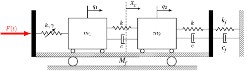
(a)

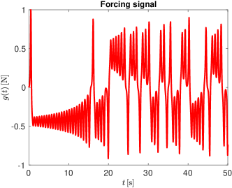
(b)

Figure 3: (a) The physical setup for the forced cart problem. (b) The chaotic forcing signal $g(t)$, generated as the $x(t)$ component of the numerically solved Lorenz system (174) with initial condition $(0,0.3,0.5)$, computed over the time interval $[0,500]$ measured in seconds. For times below $t<0$, we set $g(t)\equiv 0.$

As the unforced $\mathbf{x}=\mathbf{0}$ fixed point is asymptotically stable and the forcing in uniformly bounded, this fixed point perturbs for small enough $\left|M_{T}g(t)\right|$ into a nearby attracting anchor trajectory $x^{*}(t)$ by Theorem (1). From the asymptotic formula (14) listed in the theorem, a $5^{th}$-order approximation for $x^{*}(t)$ has the terms

$$x_{1}(t)=\int_{-\infty}^{t}e^{A(t-\tau)}f_{1}(\tau)d\tau,\qquad x_{2}(t)=0,\qquad x_{3}(t)=\int_{-\infty}^{t}e^{A(t-\tau)}\left(\begin{array}[]{c}0\\ 0\\ 0\\ -\frac{\gamma(M_{f}+m_{1})}{m_{1}M_{f}}[x_{1}^{1}(\tau)]^{3}\\ \frac{\gamma}{m_{1}}[x_{1}^{1}(\tau)]^{3}\\ 0\end{array}\right)d\tau,$$

$$x_{4}(t)=0,\hfill x_{5}(t)=\int_{-\infty}^{t}e^{A(t-\tau)}\left(\begin{array}[]{c}0\\ 0\\ 0\\ -\frac{\gamma(M_{f}+m_{1})}{m_{1}M_{f}}3[x_{1}^{1}(\tau)]^{2}x_{3}^{1}(\tau)\\ \frac{\gamma}{m_{1}}3[x_{1}^{1}(\tau)]^{2}x_{3}^{1}(\tau)\\ 0\end{array}\right)d\tau,$$ (194)

with the external forcing $f_{1}(t)=\left(0,0,0,0,0,g(t)\right)^{\mathrm{T}}$ appearing in the first-order version of the equations motion.

Utilizing that the forcing signal $g(t)$ vanishes for $t<0$, we evaluate the integrals in (194) via the trapezoidal integration scheme of MATLAB. For sufficient accuracy, we use forcing values evaluated at $10^{4}$ equally spaced times to ensure accurate numerical integration. The terms $x_{\nu}(t)$ in the expansion for $x^{*}(t)$ are then spline-interpolated in time to obtain an expression for $x^{*}(t)$ for arbitrary $t\in\left[0,500\right]$.

To compute the non-autonomous SSM coefficients, we change coordinates such that $x^{*}(t)$ serves as the origin of the transformed system (32). As a result, the matrices defined in eq. (39) are of the form

$$A^{u}=\left(\begin{array}[]{cc}\lambda_{1}&0\\ 0&\lambda_{2}\end{array}\right),\quad A^{v}=\left(\begin{array}[]{cccc}\lambda_{3}&0&0&0\\ 0&\lambda_{4}&0&0\\ 0&0&\lambda_{5}&0\\ 0&0&0&\lambda_{6}\end{array}\right),$$

with $\lambda_{1,2}=-0.0227\pm 0.3956i$ and $\lambda_{3,4}=-0.1234\pm 1.2700i$, $\lambda_{5,6}=-0.3788\pm 1.6707i$. These eigenvalues satisfy the non-resonance condition (61), and hence by Theorem 4, there exists a 2D autonomous SSM, $W_{\epsilon}(E,t)$, that admits a truncated Taylor expansion

$$v_{i}\approx\sum_{j,\mathbf{{m}=1}}^{j+|\mathbf{m}|=N}\epsilon^{j}u_{1}^{m_{1}}u_{2}^{m_{2}}h_{i}^{j\mathbf{{m}}}(t)$$ (195)

for any $N\geq 2$ in system (32). Here we choose the dimensional book-keeping parameter

$$\epsilon=\text{$\frac{\text{$\max\left|\mathbf{F}\left(t\right)\right|$}}{M_{f}+m_{1}+m_{2}}$}$$

in computing the expansion (195). As already noted, the actual ratio between external forces to internal forces along trajectories is better represented by the dimensionless forcing weakness parameter $r_{w}$.

Up to the order of truncation in eq. (195), the two-dimensional SSM-reduced order model (67) can be written in the complex coordinate $u_{1}$ as

$$\dot{u}_{1}=\lambda_{1}u_{1}+f_{u_{1}}\left(u,\sum_{j,\mathbf{{m}=1}}^{j+|m|=5}\epsilon^{j}u_{1}^{m_{1}}u_{2}^{m_{2}}\mathbf{{h}}^{j\mathbf{{m}}}(t),x_{\epsilon}(t))\right).$$ (196)

After computing the trajectory from formulas (194) up to fifth order, we use the recursive formulas in statement (i) of Theorem 4 to compute the coefficients $\mathbf{{h}}^{j\mathbf{{m}}}(t)$ in eq. (196) up to the same order recursively. Details for the coefficients in the SSM-reduced model (196) can be found in the code available from Kaundinya and Haller [27].

To assess the performance of the truncated SSM-reduced model (196) for $N=5$, we first plot the normalized mean trajectory error computed from 10 different initial conditions for $\text{{max}}||F||=0.06\,\left[N\right]$ in Fig. 4ba. We compute the dependence of this error on $\text{{max}}||F||$ in Fig. 4bb. As expected, the errors grow with $\text{{max}}||F||$ but remains an order of magnitude less than $\text{{max}}||F||$.

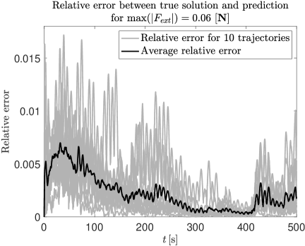
(a)

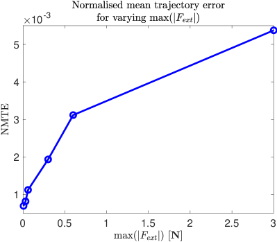
(b)

Figure 4: Error distribution of the SSM-reduced modeling error for the chaotically shaken cart example. (a) Ensemble average (black) of the mean trajectory errors (grey, normalized by the maximum of the maximal trajectory amplitude) computed from 10 initial conditions under forcing with $\text{{max}}||F||=0.06$ $\left[N\right]$. (b) The mean trajectory error under varying $\text{{max}}||F||$ on trajectories starting from the initial condition $u_{1}=u_{2}=1.2$ in all cases.

Probing larger forcing amplitudes, we still obtain accurate reduced-order models up to $\text{{max}}||F||=3\,\left[N\right]$. As an illustration, Fig. 5 uses the center-of-mass coordinate $x_{c}$ to show our $5^{th}$ order asymptotic approximation using Theorem 1 for the anchor trajectory of the chaotic SSM (blue), a simulation from the full model for a trajectory in the 2D SSM converging to the anchor point (black), and a prediction from the 2D SSM-reduced model obtained from Theorem 4 for the same trajectory (red).

In Fig. 6 (Multimedia available online), we also plot snapshots of the chaotic 2D SSM, its anchor trajectory, a trajectory from the full order model and the prediction for this trajectory from the SSM-reduced order model at three different times. Note how both the full trajectory and the predicted model trajectory synchronize with the anchor trajectory of the SSM (see Figure 6).

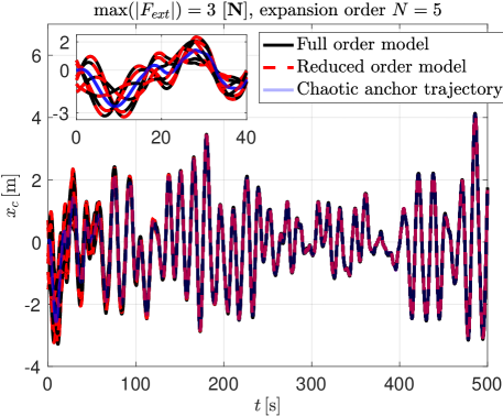
Figure 5: SSM-reduced model predictions and their verification in the chaotically forced cart example (see the text for details). The non-dimensional forcing weakness measure gives $r_{w}=7.8$, which is clearly outside the small forcing regime. We also zoom in to show the initial transient phase to highlight how the reduced order model captures the dynamics of the full order model.

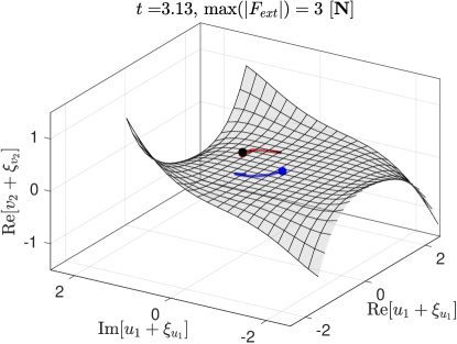
(a)

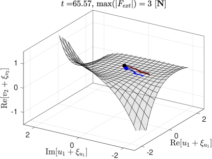
(b)

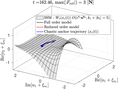
(c)

Figure 6: (a)–(c) Snapshots of the evolution of the 2D SSM, its anchor trajectory and a trajectory of the SSM-reduced model shown in the coordinates used in Theorem 4. The non-dimensional forcing weakness measure is again $r_{w}=7.8$, which is no longer small. See Movie 1 in the Supplementary Material for the full evolution. (Multimedia available online)

Finally, we would like to illustrate that the improper integrals in our asymptotic formulas for anchor trajectories and SSMs indeed converge and give correct results even for discontinuous forcing, as noted in Remark 6. To this end, we make the forcing discontinuous at 10 random points in time, as shown in Figure 7a. The same formulas for the anchor trajectory, its attached SSM and the SSM-reduced order model remain formally applicable and continue to give accurate approximations even for the relatively large forcing amplitude of $\text{{max}}||F||=3\left[\mathrm{N}\right]$, as seen in Figure 7.

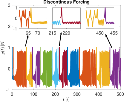
(a)

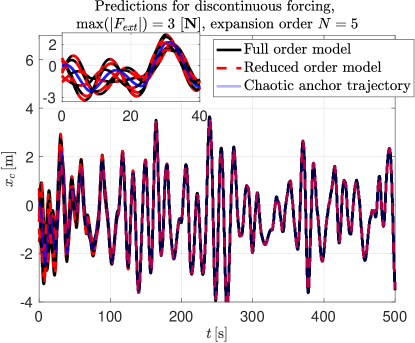
(b)

Figure 7: (a) Discontinuous chaotic forcing profile for the cart example with non-dimensional forcing weakness $r_{w}=7.8$. We set $g(t)\equiv 0$ for $t<0$. (b) Same as Fig. 5 but for the discontinuous chaotic forcing profile shown in the subplot (a).

We close this subsection with a slight modification of our example that adds more nonlinearity to the problem and underlines the utility of the higher-order approximations we have developed for the anchor trajectory (or generalized steady state) and the SSM attached to it. For brevity, we will only illustrate the need for higher-order approximations to the anchor trajectory by replacing the localized nonlinearity in eq. (81) with the more general nonlinearity

$$\mathbf{f}(\mathbf{{x},\dot{{x}}})=\left(\begin{array}[]{c}\gamma q_{1}^{3}-\gamma_{f}\frac{{m_{1}+m_{2}}}{M_{T}}\beta(\mathbf{{x}})\\ -\gamma_{f}\frac{{m_{2}}}{M_{T}}\beta(\mathbf{{x}})\\ \gamma_{f}\beta(\mathbf{{x}})\end{array}\right),\qquad\beta(\mathbf{{x}})=\Bigg{(}x_{c}-\frac{{(m_{1}+m_{2})}}{M_{T}}q_{1}-\frac{{m_{2}}}{M_{T}}q_{2}\Bigg{)}^{3}.$$ (197)

This makes the originally linear right-most spring between the cart and the wall in Fig. 3 nonlinear with cubic nonlinear stiffness coefficient $\gamma_{f}$.

First, Fig. 8a shows for $\gamma_{f}=0\mathrm{\left[N/m^{3}\right]}$ (i.e., for the linear limit of the right-most spring) the $\mathcal{O}\left(1\right)$ and $\mathcal{O}\left(11\right)$ asymptotic approximations to the anchor trajectory of the chaotic SSM using the results of Theorem 1. Already in this case, the $\mathcal{O}\left(1\right)$ approximation is noticeably improved by the $\mathcal{O}\left(11\right)$ approximation, but the $\mathcal{O}\left(1\right)$ approximation is also close to the actual generalized steady state.

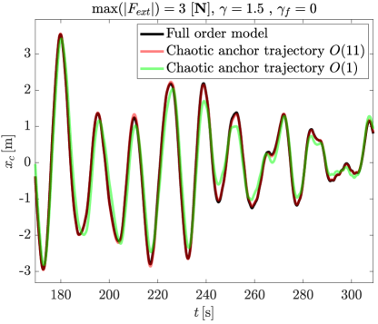
(a)

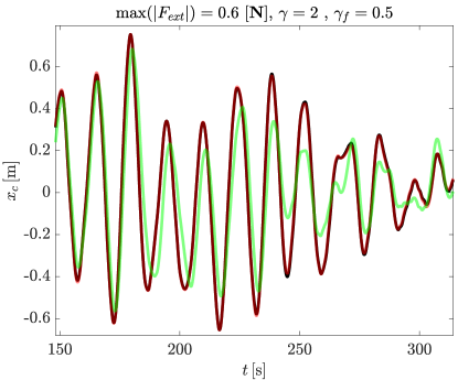
(b)

Figure 8: Leading-order and higher-order approximation of the generalized steady state of the cart system under weak chaotic forcing. (a) For $\text{{max}}||F||=3\left[\mathrm{N}\right]$ with non-dimensional forcing weakness $r_{w}=15.82$ and a linear right-most spring ($\gamma_{f}=0\mathrm{\left[N/m^{3}\right]}$). (b) For one-fifth of the forcing level in case (a) ($\text{{max}}||F||=0.6\left[\mathrm{N}\right]$, $r_{w}=6$) but for a nonlinear right-most spring ($\gamma_{f}=0.5\mathrm{\left[N/m^{3}\right]}$)

In contrast, Fig. 8b shows a case in which much smaller forcing is applied but the right-most spring is nonlinear with $\gamma_{f}=0.5\mathrm{\left[N/m^{3}\right]}$. In this case, more significant error develops between the actual anchor trajectory and its $\mathcal{O}\left(1\right)$, while the $\mathcal{O}\left(11\right)$ approximation remains indistinguishably close to the actual anchor trajectory. This example, therefore, underlines the need for higher approximations to the anchor point in the presence of stronger nonlinearities. As the SSM is attached to the anchor trajectory, the accuracy of an SSM-reduced model also depends critically on this refined approximation.

4.1.2 Slow forcing

For the same cart system shown in Fig. 3a, we select the physical parameters $m_{1}=m_{2}=1\,\mathrm{\left[kg\right]}$, $M_{f}=2\,\left[\mathrm{kg}\right]$, $k=k_{f}=1\,\,\mathrm{\left[N/m\right]}$ and $c=c_{f}=0.3\,\mathrm{\left[Ns/m\right]}$. We now slow down the previously applied chaotic forcing by replacing the external forcing vector in eq. (LABEL:eq:data_for_weakly_forced_cart) with $\mathbf{{F}(\alpha)}=\left(0,0,N_{s}g(\alpha)\right)^{\mathrm{T}}.$ We select this forcing to be of large amplitude by letting $N_{s}=10$ and consider the phase range $\alpha\in[0,6]$. In our analysis, we will start with the minimal forcing speed $\epsilon=\dot{\alpha}=0.001$, for which obtain the non-dimensional forcing speed $r_{s}=0.72$ from the second formula in (176). This qualifies as moderately slow external forcing relative to the speed of variation of internal forces along unperturbed trajectories. In contrast, for the maximal forcing speed $\epsilon=\dot{\alpha}=0.008$ we will consider, we obtain $r_{s}=7.26$, which can no longer be considered slow. Again, of particular interest will be how our asymptotic formulas for adiabatic SSMs and their anchor points perform in the latter case, which is clearly faster than what is normally considered slowly varying in perturbation theory.

We start by solving for the fixed point $\mathbf{x}_{0}(\alpha)$ of the system under static forcing, as defined by the algebraic equation in eq. (109). In the present example, this amounts to solving the equation

$$\mathbf{{K}}\mathbf{\mathbf{x}}_{0}+\mathbf{f}(\mathbf{x}_{0},\mathbf{0})=\mathbf{{F}}(\alpha),$$ (198)

which is obtained from the general forced equation of motion (175). We solve this nonlinear algebraic equation for the selected range of $\alpha$ values by Newton iteration.

Once $x_{0}(\alpha)$ is available numerically, we evaluate the recursive formula (114) up to order $N=3$ to obtain

$$x_{1}(\alpha)=A^{-1}(\alpha)x^{\prime}_{0}(\alpha),\quad x_{2}(\alpha)=A^{-1}(\alpha)\left(x^{\prime}_{1}(\alpha)-\left(\begin{array}[]{c}0\\ 0\\ 0\\ -\frac{\gamma(M_{f}+m_{1})}{m_{1}M_{f}}3[x_{1}^{1}(\alpha)]^{2}x_{0}^{1}(\alpha)\\ \frac{\gamma}{m_{1}}3[x_{1}^{1}(\alpha)]^{2}x_{0}^{1}(\alpha)\\ 0\end{array}\right)\right),$$

$$x_{3}(\alpha)=A^{-1}(\alpha)\left(x^{\prime}_{2}(\alpha)-\left(\begin{array}[]{c}0\\ 0\\ 0\\ -\frac{\gamma(M_{f}+m_{1})}{m_{1}M_{f}}([x_{1}^{1}(\alpha)]^{3}+6x_{1}^{1}(\alpha)x_{0}^{1}(\alpha)x_{2}^{1}(\alpha))\\ \frac{\gamma}{m_{1}}([x_{1}^{1}(\alpha)]^{3}+6x_{1}^{1}(\alpha)x_{0}^{1}(\alpha)x_{2}^{1}(\alpha))\\ 0\end{array}\right)\right).$$

Having computed this approximation for the anchor trajectory, we change to the coordinates defined in eq. (118). In those coordinates, we compute the $\alpha$-dependent matrices defined in eq. (132) numerically. Their general form in the present examples is

$$A^{u}=\left(\begin{array}[]{cc}\lambda_{1}(\alpha)&0\\ 0&\lambda_{2}(\alpha)\end{array}\right),\quad A^{v}=\left(\begin{array}[]{cccc}\lambda_{3}(\alpha)&0&0&0\\ 0&\lambda_{4}(\alpha)&0&0\\ 0&0&\lambda_{5}(\alpha)&0\\ 0&0&0&\lambda_{6}(\alpha)\end{array}\right).$$

To perturb from this frozen-time limit, we set $\alpha=\epsilon\Omega t$ and $\Omega=1\text{{Hz}}$ to make the small parameter $\epsilon$ non-dimensional.

We set $N$= 3 and solve for all the $\alpha$ dependent coefficients in the expansion of the 2D slow chaotic SSM by solving a recursive linear algebraic equations (139) order by order. We find that all 28 coefficients that describe the SSM up to cubic order are nonzero. An important numerical step used in this task is to perform differentiation with respect to $\alpha$. For this purpose, we first need to re-orient the unit eigenvectors originally returned by MATLAB for specific values of $\alpha$ to make these eigenvectors smooth functions of $\alpha.$ We then perform a central finite differencing which includes 4 adjacent points in the $\alpha$ direction. We finally employ the Savitzky–Golay filtering function of MATLAB to smoothen the results obtained from finite differencing an already finite-differenced signal.

To illustrate the ultimate accuracy of these numerical procedures, Table 1 shows the normalized mean trajectory error for predictions from two different SSM-reduced models. We see that under increasing $\epsilon$ (i.e., faster forcing), the errors still remain an order-of-magnitude smaller then $\epsilon$.

	$O(\epsilon,j=1,|m|=3)$	$O(\epsilon^{3},j+|m|=3)$
$\epsilon=0.001$   ($r_{s}=0.72$)	$9.8\times 10^{-5}$	$7.2\times 10^{-6}$
$\epsilon=0.008$   ($r_{s}=7.26$)	$6.4\times 10^{-3}$	$7.8\times 10^{-4}$
$\epsilon=0.010$   ($r_{s}=8.66$)	$1.1\times 10^{-2}$	$2.9\times 10^{-3}$

Table 1: Normalized mean trajectory error for predictions from two different SSM-reduced models under different $\epsilon$ values. The corresponding non-dimensional forcing speed $r_{s}$ is also shown for each listed value of $\epsilon$.

As we did for weak forcing, we track the center of mass coordinate $x_{c}$ to test the accuracy of our asymptotic formulas up to order $N=3$ for $\epsilon=0.008$ in Fig. 9. Note how this cubic-order approximation of the SSM-reduced model already tracks the full solution closely. Finally, as in the weakly forced case, we also plot in Fig. 10 snapshots of the evolution of the slow anchor trajectory, the attached chaotic SSM, a simulated full-order trajectory and its prediction from the same initial condition based on the SSM-reduced dynamics (Multimedia available online). These snapshots further confirm the accuracy of our analytic approximation formulas, now in several coordinate directions.

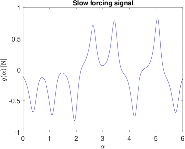
(a)

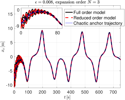
(b)

Figure 9: (a) Slow chaotic forcing signal $g(\epsilon t)$ for the cart example for $\epsilon=0.008$, which amounts to $r_{s}=7.26$. (b) Assessment of the accuracy of the anchor trajectory and the reduced dynamics of the slow chaotic SSM in the cart example, based on the history of the $x_{c}(t)$ coordinate of the center of mass.

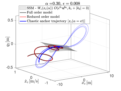
(a)

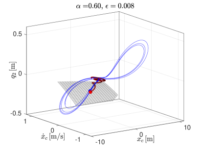
(b)

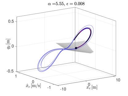
(c)

Figure 10: (a)–(c) Snapshots of the evolution of the slow chaotic SSM, its anchor trajectory, the true solution of the full system and the SSM-reduced model prediction for the true solution of the chaotically shaken cart, all represented in the physical coordinates $[q_{2},x_{c},\dot{{x}}_{c}]$. The non-dimensional forcing speed is $r_{s}=7.26$. See Movie 2 in the Supplementary Material for the full evolution. (Multimedia available online)

4.2 Example 2: Chaotically forced bumpy rail

4.2.1 Weak forcing

The physical setup of our second example, a particle moving on a shaken rail with a bump in the middle, is shown in Fig. 11a. A major difference from our previous mechanical example is that the origin of the unforced system is now an unstable, saddle-focus-type fixed point. Therefore, under weak chaotic forcing, a nearby chaotic SSM of mixed-mode type is expected to arise attached to a saddle-focus-type chaotic anchor trajectory.

We use the center of mass position $x_{c}$ and the relative position $x$ of the smaller mass $m$ as generalized coordinates. In terms of these coordinates, the quantities featured in the general equation of motion (173) take the form

$$\mathbf{M}={\scriptscriptstyle\left(\begin{array}[]{cc}M_{f}+m&0\\ 0&\frac{mM_{f}}{m+M_{f}}\end{array}\right)},\quad\mathbf{K}={\scriptstyle\left(\begin{array}[]{cc}k_{f}&-k_{f}\frac{m}{M_{f}+m}\\ -k_{f}\frac{m}{M_{f}+m}&-4\beta a^{2}mg+k_{f}\frac{m^{2}}{(M_{f}+m)^{2}}\end{array}\right)},$$

$$\mathbf{C}={\scriptstyle\left(\begin{array}[]{cc}c_{f}&-c_{f}\frac{m}{M_{f}+m}\\ -c_{f}\frac{m}{M_{f}+m}&c+c_{f}\frac{m^{2}}{(M_{f}+m)^{2}}\end{array}\right)},\quad\mathbf{f}(\mathbf{x},\dot{\mathbf{x}})={\scriptstyle\left(\begin{array}[]{c}0\\ 4g\beta mx^{3}+16m\beta^{2}a^{4}x\dot{{x}}^{2}\end{array}\right)},$$

$$\mathbf{F}(t)={\scriptscriptstyle\left(\begin{array}[]{c}(m+M_{f})g(t)\\ 0\end{array}\right)},$$

with for the coordinate vector $\mathbf{x}=\left(x_{c},x\right)^{\mathrm{T}}$. The parameter $\beta$ controls the height of the bumpy rail and $a$ the distance to the wells. The parameter $c$ models linear damping of the mass $m$ due to the rail. The velocity-dependent nonlinearity $\mathbf{f}(\mathbf{x},\dot{\mathbf{x}})$ is the result of expanding the exact equations of motion with respect to the height of the rail and keeping only the leading-order nonlinearities.

We set $m=1\,\mathrm{\left[kg\right]}$, $M_{f}=4\mathrm{\,\left[kg\right]}$, $k_{f}=1\,\mathrm{\left[N/m\right]}$, $c_{f}=c=0.3$ $\left[\mathrm{Ns/m}\right]$, $a=0.3\,\left[\mathrm{m}\right]$, $\beta=\frac{1}{5a^{3}}$ and $g=9.8$ $\left[\mathrm{m/s^{2}}\right]$ . The forcing signal $g(t)$ will be the same as in the cart example. We scale the chaotic forcing signal in a way that the non-dimensional forcing weakness measure defined in formula ((176)) gives $r_{w}=44.6$ when evaluated on the phase space region containing the trajectories used in our analysis. Therefore, the external force here is large relative to the internal forces of the system.

This forcing magnitude is outside the small range in which Theorem 4 strictly guarantees the existence of a saddle-type anchor trajectory for a mixed-mode chaotic SSM in this problem. We nevertheless evaluate our asymptotic expansions for the anchor trajectory, as those expansions hold as long as the SSM smoothly persist under increasing forcing. Specifically, a cubic-order approximation $x^{*}(t)\approx\sum_{\nu=1}^{3}x_{\nu}(t)$ for the anchor trajectory $x^{*}(t)$ from formula (14) requires the functions

$$x_{1}(t)=\int_{-\infty}^{\infty}G(t-\tau)f_{1}(\tau)d\tau,\qquad x_{2}(t)\equiv 0,$$

$$x_{3}(t)=\int_{-\infty}^{\infty}G(t-\tau)\left(\begin{array}[]{c}0\\ 0\\ 0\\ -4g(1+\frac{m}{M})\beta[x_{1}^{2}(\tau)]^{3}-16a^{4}(1+\frac{m}{M})\beta^{2}x_{1}^{2}(\tau)[x_{1}^{4}(\tau)]^{2}\end{array}\right)d\tau,$$

with the Green’s function $G(t)$ defined in formula (13) for saddle-type anchor trajectories. The external forcing appears now as $f_{1}(t)=\left(0,g(t),0,0\right)^{\mathrm{T}}$ in the first-order formulation of the equation of motions. We calculate these integrals using the same numerical methodology as in our first cart example. In this example, the calculation of $G(t-\tau)$ from (13) involves the matrices

$$A^{u}=\left(\begin{array}[]{cc}\lambda_{1}&0\\ 0&\lambda_{2}\end{array}\right),\quad A^{v}=\left(\begin{array}[]{cc}\lambda_{3}&0\\ 0&\lambda_{4}\end{array}\right),$$

where the eigenvalues of the unforced saddle-focus-type fixed point at the origin are $\lambda_{1}=5.5196$, $\lambda_{2}=-5.9094$, $\lambda_{3,4}=-0.0301\pm 0.4465i$. The 2D non-autonomous SSM can be constructed as a graph over the mixed-mode tangent space corresponding to the real eigenvalues $\lambda_{1}$ and $\lambda_{2}$.

Without listing the details here, we also perform a similar calculation for the two attracting anchor trajectories created by the chaotic forcing from the two asymptotically stable fixed points of the unperturbed system that lie at the two bottom points of the bumpy rail. These two stable anchor trajectories will represent two chaotic attractors for the forced system. Trajectories initialized near the unstable anchor trajectory on its attached 2D mixed-mode SSM will converge to one of these chaotic attractors. This is indeed observable in Fig. 11b, in which we launch several trajectories near the unstable anchor trajectory (red) within the 2D mixed-mode SSM approximated up to cubic order. These trajectories then converge to one of the two predicted attracting chaotic anchor trajectories (blue) which we have computed up to cubic order of accuracy from our formulas.

The instability of the anchor trajectory perturbing from the origin makes it challenging to verify the accuracy of our local expansion (139) for the 2D mixed-mode SSM attached to this trajectory. We can nevertheless verify the local accuracy for these formulas by tracking nearby trajectories launched from the predicted 2D SSM and confirm in Fig. 12 (Multimedia available online) that those trajectories evolve together with the predicted SSM until ejected from a neighborhood of the unstable anchor trajectory.

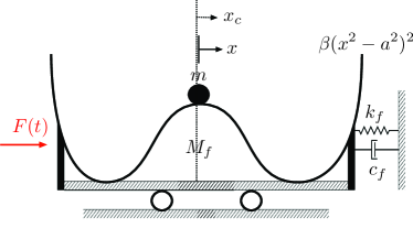
(a)

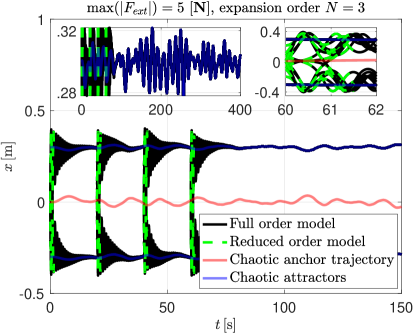
(b)

Figure 11: (a) Setup for the chaotically forced bumpy real example (b) Plots of 16 initial conditions on local mixed-mode non-autonomous 2D SSM, released at four different times. The left inset shows how the transient behavior of the full system matches those of the anchor trajectories calculated from our theory. The right inset shows fast convergence of the full solution to the anchor trajectories together with local predictions of the reduced order model. The non-dimensional forcing weakness measure in this example is $r_{w}=44.6$.

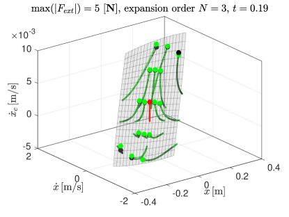
(a)

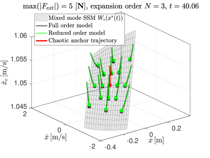
(b)

Figure 12: (a)–(b) SSM dynamics in the (not so) weakly forced bumpy rail example. Shown are snapshots of the predicted 2D mixed-mode SSM (grey), its anchor trajectory (red), trajectories predicted by the SSM-reduced model (green) and full system simulations of trajectories launched from the same initial conditions (black). The non-dimensional forcing weakness measure is again $r_{w}=44.6$. See Movie 3 in the Supplementary Material for the full evolution. (Multimedia available online)

4.2.2 Slow forcing

In the same bumpy rail problem but now with height $\beta=\frac{1}{10^{3}}$, we rescale the forcing in time to make it slowly varying. The slow forcing vector is given by $\mathbf{{F}(\alpha)}=\left(\begin{array}[]{c}N_{s}g(\alpha)\\ 0\end{array}\right)$ with $N_{s}=3$ and the range of interest is $\alpha\in[0,6].$ We will perform simulations for the forcing speed $\epsilon=\dot{\alpha}=0.01$, which yields the non-dimensional forcing speed measure $r_{s}=1.22$, signaling moderately fast forcing.

As in our first example, we compute the zeroth order term $x_{0}(\alpha)$ in the expansion of the slow anchor trajectory for the SSM by solving an algebraic equation of the form (198) by Newton iteration.

$$\mathbf{{K}}\mathbf{{x}}_{0}+\mathbf{f}(\mathbf{x}_{0},\mathbf{0})=\mathbf{{F}}(\alpha).$$

Up to cubic order, the expansion (114) for the slow, unstable anchor trajectory perturbing from the origin under the slow forcing can be written as

$$x_{1}(\alpha)=A^{-1}(\alpha)x^{\prime}_{0}(\alpha),$$

$$x_{2}(\alpha)={\scriptstyle A^{-1}(\alpha)\left(x^{\prime}_{1}(\alpha)-\left(\begin{array}[]{c}0\\ 0\\ 0\\ (1+\frac{m}{M})\left(-12g\beta x_{0}^{2}(\alpha)[x_{1}^{2}(\alpha)]^{2}-16a^{4}\beta^{2}x_{0}^{2}(\alpha)[x_{1}^{4}(\alpha)]^{2}\right)\end{array}\right)\right)},$$

$$x_{3}(\alpha)={\scriptscriptstyle{\scriptstyle A^{-1}(\alpha)\left(x^{\prime}_{2}(\alpha)-\left(\begin{array}[]{c}0\\ 0\\ 0\\ (1+\frac{m}{M})\times\\ {\scriptstyle\left(-4g\beta\left([x_{1}^{2}(\alpha)]^{3}+6x_{0}^{2}(\alpha)x_{1}^{2}(\alpha)x_{2}^{2}(\alpha)\right)-16a^{4}\beta^{2}\left(x_{1}^{2}(\alpha)[x_{1}^{4}(\alpha)]^{2}+2x_{0}^{2}(\alpha)x_{1}^{4}(\alpha)x_{2}^{4}(\alpha)\right)\right)}\end{array}\right)\right)}}.$$

With this approximation for the anchor trajectory at hand, we can change to the coordinates defined in eq. (118). In those coordinates, we compute the $\alpha$-dependent matrices defined in eq. (132) now arise as

$$A^{u}=\left(\begin{array}[]{cc}\lambda_{1}(\alpha)&0\\ 0&\lambda_{2}(\alpha)\end{array}\right),\quad A^{v}=\left(\begin{array}[]{cc}\lambda_{3}(\alpha)&0\\ 0&\lambda_{4}(\alpha)\end{array}\right),$$

where we again set $\alpha=\epsilon\Omega t$ with $\Omega=1\text{ {Hz}}$, as in our first example.

As in the weakly forced version of this example, we plot the predictions from the 2D SSM-reduced order model and compare it to simulations of the full system in Fig. 13a (Multimedia available online). We again see close agreement of the reduced dynamics with the true solution in the vicinity of the slow, unstable anchor trajectory, prior to the convergence of the trajectories to the two stable, chaotic anchor trajectories arising from the two stable unforced equilibria along the rail. Finally, as in our first example, we show snapshots of the projected 2D slow, mixed-mode SSM along with some trajectories of its restricted dynamics. These agains stay close locally to trajectories of the full system that are launched from the same initial conditions, thereby confirming the expectations put forward in Remark 9.

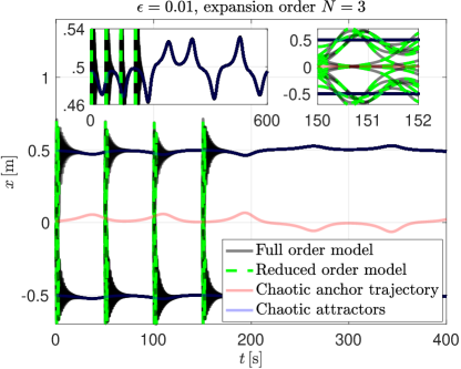
(a)

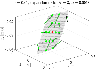
(b)

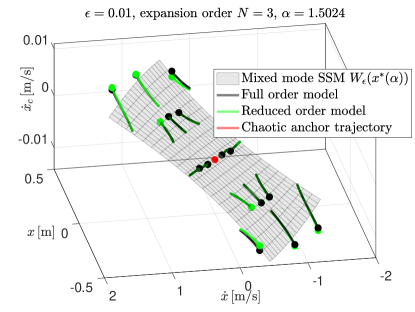
(c)

Figure 13: (a)–(c) Same as Fig. 12, but now for moderately slow chaotic forcing with non-dimensional forcing speed measure $r_{s}=1.22$. See Movie 4 in the Supplementary Material for the full evolution. (Multimedia available online)

5 Conclusions

In this paper, we have derived existence results for spectral submanifolds (SSMs) in non-autonomous dynamical systems that are either weakly non-autonomous or slowly varying (adiabatic). While our exact proofs for these SSMs results only cover weak enough or slow enough time dependence, the invariant manifolds we obtain are structurally stable and hence are persistent away from these limits. Under further nonresonance conditions, the manifolds and their reduced dynamics also admit asymptotic expansions up to any finite order for which we present recursive formulas. These formulas suggest that one of the non-autonomous SSMs is as smooth as the original dynamical system, just as primary SSMs are known to be in the autonomous case reviewed in the Introduction. MATLAB implementations of our recursive formulas for the examples treated here are available from Kaundinya and Haller [27].

In our results, weakly forced SSMs are guaranteed to exist under uniformly bounded forcing. This restriction is expected because unbounded perturbations to an autonomous limit of a dynamical system will generally wipe out any structure identified in that limit. For adiabatic SSMs, the uniformity of the forcing magnitude is replaced by the uniformity of the strength of hyperbolicity along the anchor trajectory of the SSM in the limit of frozen time.

In the weakly forced case, the SSMs emanate from unique, uniformly bounded hyperbolic anchor trajectories. Our expansions for these anchor trajectories are of independent interest as they provide formal approximations of the generalized steady state response of any nonlinear system subject to moderate but otherwise arbitrary time-dependent forcing. In finite-element simulations under aperiodic forcing, such steady states have been assumed to exist but their computation tends to involve lengthy simulations of randomly chosen initial conditions until they have reached a (somewhat vaguely defined) statistical steady state.

Even with today’s computational power, such simulations are still prohibitively long due to the small damping of typical structural materials, the high degrees of freedom of the models used, and the costly evaluations of nonlinearities arising from complex geometries and multi-physics. With the explicit recursive formulas we obtained here, one can now directly approximate these generalized steady states without lengthy simulations.

For these asymptotic formulas to converge, the forcing does not actually have to be uniformly bounded: it may grow temporally unbounded in a compact neighborhood of the origin as long as the improper integrals in the statements of Theorems 2 and 4 converge. To the best of our knowledge, such explicit, readily computable asymptotic expansions for time-dependent steady states have been unavailable in the literature even for time-periodic or time-quasiperiodic forcing, let alone time-aperiodic forcing. Weak or slow time-periodic and time-quasi-periodic forcing is also covered by these formulas as special cases.

Our existence results for SSMs assume temporal smoothness for the dynamical system and hence do not strictly cover the case of random forcing with continuous paths. Our approximation formulas, however, are formally applicable (i.e., the improper integrals in them converge) for much broader forcing types, including mildly exponentially growing or temporally discontinuous forcing. Therefore, the results in this paper provide formal nonlinear model reduction formulas that can be implemented as approximations for all forcing types arising in practice.

The simple examples considered here already illustrate the ability of our asymptotic formulas to work under various forcing types, including chaotic and discontinuous forcing. Our weakly non-autonomous SSM theory is expected to be helpful in model reduction for structural vibrations problems in which so far time-periodic and time-quasiperiodic SSMs have been constructed. An application of our adiabatic SSM theory is already underway in the model-predictive control of soft robots, wherein the target trajectories of the robot generally have a much slower time scale than the highly damped robot itself.

Going from the simple, illustrative examples treated here to finite-element problems with temporally aperiodic forcing will require no further theoretical development. Indeed, the existence and smoothness results derived in this paper are valid in arbitrarily high (finite) dimensions. However, a computational reformulation will be required to make these results directly applicable to second-order mechanical systems without the need to convert them to first-order systems with diagonalized linear parts. The development of such a reformulation using the approach of Jain and Haller [24] is currently underway.

Acknowledgements

We are grateful to Christian Pötzsche for very helpful and detailed explanations and references on the continuity of the dichotomy spectrum for non-autonomous differential equations. We are also grateful to Martin Rasmussen and Peter Kloeden for helpful references on non-autonomous invariant manifolds.

Appendix A Proof of Theorems 1 and 2

A.1 Proof of Theorem 1: Existence and regularity of a hyperbolic anchor trajectory

We first recall a result of Palmer [35], reformulated from Hartman [22], for a general non-autonomous ODE of the form

$$\dot{x}=A(t)x+f(x,t,p),$$ (A1)

where $A(t)$ and $f(x,t,p)$ are $C^{0}$ functions of their arguments; $\left|f(x,t,p)\right|\leq\mu$ is assumed to hold for a constant $\mu>0$ and for all $x\in\mathbb{R}^{n}$ and $t\in\mathbb{R}$; $f(\,\cdot\,,t,p)$ admits a global Lipschitz constant $L>0$ for all times $t$; and $p\in\mathbb{R}^{m}$ is a parameter vector.

Assume that the linearization

$$\dot{x}=A(t)x$$ (A2)

of system (A1) has an exponential dichotomy, i.e., there exists a fundamental matrix solution $\Phi(t)$ of (A2), constants $K,\kappa>0$ and a projection $P$ (with $P^{2}=P)$ such that

$$\left|\Phi(t)P\Phi^{-1}(s)\right| \leq Ke^{\kappa\left(t-s\right)},\quad t\geq s,$$

$$\left|\Phi(t)\left(I-P\right)\Phi^{-1}(s)\right| \leq Ke^{\kappa\left(t-s\right)},\quad s\geq t.$$ (A3)

This condition guarantees that the $x=0$ solution of the linearized system (A2) is hyperbolic, i.e., has well-defined stable and/or unstable subbundles (no neutrally stable directions). Finally, assume that

$$4LK\leq\kappa.$$ (A4)

Under these assumptions, there exists a unique, globally bounded solution $x^{*}(t;p)$ of the nonlinear system (A1) that satisfies

$$\left|x^{*}(t;p)\right|\leq 2K\mu/\kappa,\quad t\in\mathbb{R},$$ (A5)

as shown in Lemma 1 of Palmer [35]). Furthermore, $x^{*}(t;p)$ is continuous in the parameter $p$. (If $f$ is smooth in its arguments, then the continuity of $x^{*}(t;p)$ in $p$ can be strengthened to smooth dependence on $p$ using more general results for the persistence of non-compact, normally hyperbolic invariant manifolds; see Eldering [12]). Such a strengthened version, however, would not be specific enough about the norm of $\left|x^{*}(t;p)\right|$ to the extent given in (A5).) Note that $x^{*}(t;p)$ takes over the role of $x=0$ as a unique, uniformly bounded solution under nonzero $f(x,t,p)$. The result of Palmer [35] quoted above makes no assumption on $f(x,t,p)$ containing only nonlinear terms, and hence $f(x,t,p)$ is allowed to be an arbitrary perturbation to the linear ODE (A2), as long as it is uniformly bounded and uniformly Lipschitz.

The uniform boundedness conditions (A4)-(A5) will not be satisfied in realistic applications. Nevertheless, one can still use the above results in such applications using smooth cut-off functions (see, e.g., Fenichel [14]) that make $f(x,t,p)$ vanish for all $t\in B_{\delta}$ outside a small ball $B_{\delta}\subset\mathbb{R}^{n}$. The latter classic tool from invariant manifold theory is, however, only applicable here if the predicted hyperbolic trajectory $x^{*}(t;p)$ lies inside $B_{\delta}$, where the cut-off right-hand side and the original right-hand side of (A1) still coincide.

To ensure this, we consider a $\delta$-ball $B_{\delta}\subset\mathbb{R}^{n}$ around $x$ and define the uniform bound $\mu(\delta)$ and uniform Lipschitz constant $L(\delta)$ as

$$\mu(\delta)=\max_{x\in B_{\delta}}\left|f(x,t,p)\right|,\qquad\left|f(x,t,p)-f(\tilde{x},t,p)\right|\leq L(\delta)\left|x-\tilde{x}\right|,\quad x,\tilde{x}\in B_{\delta}.$$ (A6)

Assume further that these bounds satisfy

$$\frac{2K\mu(\delta)}{\kappa}\leq\delta,\quad L(\delta)\leq\frac{\kappa}{4K},$$ (A7)

which assures that assumption (A4) holds and also that the predicted $x^{*}(t;p)$ falls in $B_{\delta}$ by the estimate (A5). Note that the inequalities in (A7) will always hold for $\delta>0$ small enough if $f(x,t,p)$ is only composed of terms that are nonlinear in $x$. Indeed, in that case, we can select $\mu(\delta)=\mathcal{O}\left(\delta^{2}\right)$ and $L(\delta)=\mathcal{O}\left(\delta\right)$ for all $x\in B_{\delta}$, and hence the inequalities in (A7) are satisfied for small enough $\delta$, given that $K,\kappa>0$ do not depend on $\delta$.

We now apply the above refined persistence result in the setting of the perturbed nonlinear system (1) by letting

$$A(t)=A,\qquad f(x,t,p)=f_{0}(x)+f_{1}(x,t),$$ (A8)

and assume a separate uniform Lipschitz constant $L_{1}(\delta)$ for $f_{1}(x,t)$ satisfying

$$\left|f_{1}(x,t)-f_{1}(\tilde{x},t)\right|\leq L_{1}(\delta)\left|x-\tilde{x}\right|,\quad x,\tilde{x}\in B_{\delta}.$$

By our hyperbolicity assumption on the $x=0$ fixed point, we can select the constant $\kappa>0$ so that

$$\kappa<\min_{1\leq j\leq n}\left|\mathrm{Re}\lambda_{j}\right|.$$ (A9)

We can also bound within $B_{\delta}$ the nonlinear term $f_{0}$ and its spatial derivative as

$$\left|f_{0}(x,p)\right|\leq K_{1}\delta^{2},\qquad\left|\partial_{x}f_{0}(x)\right|\leq K_{2}\delta,\qquad x\in B_{\delta},$$ (A10)

where $K_{1},K_{2}>0$ are appropriate constants. Additionally, we can specifically choose $K_{2}=\max_{x\in B_{\delta}}\left|\partial_{x}f_{0}(x)\right|$ by the mean value theorem. Given these bounds, the constants in formulas (A6) can be estimated as

$$\mu(\delta)\leq K_{1}\delta^{2}+\left|f_{1}(x,t)\right|,\quad L(\delta)\leq L_{1}(\delta)+K_{2}\delta,\quad x\in B_{\delta}.$$ (A11)

Based on the inequalities (A11), we see that assumptions (A7) are satisfied if

$$\frac{2K\left(K_{1}\delta^{2}+\left|f_{1}(x,t)\right|\right)}{\kappa}\leq\delta,\quad L_{1}(\delta)+K_{2}\delta\leq\frac{\kappa}{4K},\qquad x\in B_{\delta},\quad t\in\mathbb{R},$$

or, equivalently, if

$$\left|f_{1}(x,t)\right|\leq\frac{\kappa\delta}{2K}-K_{1}\delta^{2},\qquad L_{1}(\delta)\leq\frac{\kappa}{4K}-K_{2}\delta,\qquad x\in B_{\delta},\quad t\in\mathbb{R}.$$ (A12)

We stress again that these conditions do not have to hold globally for all $x$, only for $x\in B_{\delta}$, but they must hold uniformly within $B_{\delta}$ for all times. This follows because we can apply the $C^{\infty}$ cutoff procedure mentioned above to the whole right-hand side of (A1), including $f_{1}(x,t)$. Based on these considerations and using the inequalities in eq. (A10), we obtain statement (i) of Theorem 1.

Statement (ii) of Theorem 1 follows from the smooth dependence of $x^{*}(t;p)$ on the parameter vector $p$, as shown by Palmer [35].

A.2 Proof of Theorem 2: Approximation of the anchor trajectory $x^{*}(t)$

First, we introduce a perturbation parameter $\epsilon\geq 0$ and rewrite the full non-autonomous system (1) as

$$\dot{x}=Ax+f(x,t;\epsilon),\quad f(x,t;\epsilon)=f_{0}(x)+\epsilon\tilde{f}_{1}(x,t).$$ (A13)

By the smooth dependence of the uniformly bounded hyperbolic solution $x^{*}(t)$ on parameters, we can seek this solution in the form of a Taylor expansion

$$x^{*}(t)=\sum_{\nu\geq 1}\epsilon^{\nu}\xi_{\nu}(t),$$ (A14)

with Taylor coefficients $\xi_{\nu}(t)$ that are uniformly bounded in time. By statement (ii) of Theorem (1), such a formal Taylor expansion in $\epsilon$ is justified up to any finite order, although may not necessarily converge.

Substitution of the expansion (A14) into eq. (A13) gives

$$\sum_{j\geq 1}\epsilon^{j}\dot{\xi}_{j}(t) =\sum_{j\geq 1}\epsilon^{j}A\xi_{j}(t)+f\left(x_{\epsilon}(t),t;\epsilon\right).$$ (A15)

Equating equal powers of $\epsilon$ on both sides yields the system of differential equations

$$\dot{\xi}_{\nu}(t)=A\xi_{\nu}(t)+\frac{1}{\nu!}\left.D_{\epsilon}^{\nu}f\left(x_{\epsilon}(t),t;\epsilon\right)\right|_{\epsilon=0}.$$ (A16)

Note that the term formally containing $\xi_{\nu}(t)$ in $\left.D_{\epsilon}^{\nu}f\left(x_{\epsilon}(t),t;\epsilon\right)\right|_{\epsilon=0}$ is

$$\nu!\left[D_{x}f_{0}(x_{\epsilon}(t))+\epsilon\tilde{f}_{1}\left(x_{\epsilon}(t),t\right)\right]_{\epsilon=0}\xi_{\nu}(t)\equiv 0,$$

because $f_{0}(x)=\mathcal{O}\left(\left|x\right|^{2}\right)$ and $x_{0}(t)\equiv 0$. Therefore, the right-hand side of eq. (A16) only depends on $\xi_{1}(t),\ldots,\xi_{\nu-1}(t)$, which makes the whole system of equations a recursively solvable sequence of inhomogeneous, linear, constant-coefficient system of ODEs. The recursive solutions are of the form

$$\xi_{\nu}(t) =e^{A\left(t-t_{0}\right)}\xi_{\nu}(t_{0})+\frac{1}{\nu!}\int_{t_{0}}^{t}e^{A\left(t-\tau\right)}\left.D_{\epsilon}^{\nu}f\left(\sum_{j=1}^{\nu-1}\epsilon^{j}\xi_{j}(\tau),\tau;\epsilon\right)\right|_{\epsilon=0}d\tau,\quad\nu\geq 1.$$ (A17)

Assume first, for simplicity, that the $x=0$ fixed point is asymptotically stable for $\epsilon=0$, and hence

$$\mathrm{Re}\left[\mathrm{spect}\left(A\right)\right]\subset\left(-\infty,0\right).$$ (A18)

In that case, by the uniform boundedness of $\xi_{1}(t_{0})$ for all $t_{0}\in\mathbb{R}$, we can take the $t_{0}\to-\infty$ limit in (A17) to obtain

$$\xi_{\nu}(t) =\frac{1}{\nu!}\int_{-\infty}^{t}e^{A\left(t-\tau\right)}\left.D_{\epsilon}^{\nu}f\left(\sum_{j=1}^{\nu-1}\epsilon^{j}\xi_{j}(\tau),\tau;\epsilon\right)\right|_{\epsilon=0}d\tau,\quad\nu\geq 1.$$ (A19)

To obtain a more explicit recursive formula for $\xi_{\nu}(t)$ for general $\nu$ that is suitable for direct numerical implementation, we will use the multi-variate Faá di Bruno formula of Constantine and Savits [10] for higher-order derivatives of composite functions. To recall the general form of this formula, we first consider a general composite function $H\colon\mathbb{R}^{p}\to\mathbb{R}$, defined as

$$H(x_{1},\ldots,x_{p})=f\left(g^{1}(x_{1},\ldots,x_{p}),\ldots,g^{m}(x_{1},\ldots,x_{p})\right),$$ (A20)

and introduce the nonnegative multi-index $\mathbf{\boldsymbol{\nu}}$ and related notation as

$$\mathbf{\boldsymbol{\nu}}=\left(\nu_{1},\ldots,\nu_{p}\right)\in\mathbb{N}^{p},\quad\left|\mathbf{\boldsymbol{\nu}}\right|=\sum_{i=1}^{p}\nu_{i},\quad\mathbf{\boldsymbol{\nu}}!=\prod_{i=1}^{p}\left(\nu_{i}!\right),\quad D_{\mathbf{x}}^{\mathbf{\boldsymbol{\nu}}}=\frac{\partial^{\left|\mathbf{\boldsymbol{\nu}}\right|}}{\partial x_{1}^{\nu_{1}}\cdots\partial x_{p}^{\nu_{p}}}.$$

We also introduce an ordering relation on $\mathbb{N}^{p}$ for arbitrary $\mathbf{\boldsymbol{\mu}},\mathbf{\boldsymbol{\nu}}\in\mathbb{N}^{p}$ such that $\mathbf{\boldsymbol{\nu}}\prec\mathbf{\boldsymbol{\mu}}$ holds provided one of the following is satisfied:

(i) $\left|\mathbf{\boldsymbol{\mu}}\right|<\left|\mathbf{\boldsymbol{\nu}}\right|$

(ii) $\left|\mathbf{\boldsymbol{\mu}}\right|=\left|\mathbf{\boldsymbol{\nu}}\right|$ and $\mu_{1}<\nu_{1}$ or

(iii) $\left|\mathbf{\boldsymbol{\mu}}\right|=\left|\mathbf{\boldsymbol{\nu}}\right|$ and $\mu_{1}=\nu_{1},\ldots\mu_{k}=\nu_{k},\mu_{k+1}<\nu_{k+1}$ for some $1\leq k<p.$

Finally, for any $\mathbf{\boldsymbol{\mu}},\boldsymbol{\gamma}\in\mathbb{N}^{p}$ and $s\in\mathbb{N}^{+}$, we define the index set

$$p_{s}\left(\mathbf{\boldsymbol{\nu}},\boldsymbol{\gamma}\right)=\left\{\left(\mathbf{k}_{1},\ldots,\mathbf{k}_{s},\boldsymbol{\ell}_{1},\ldots,\boldsymbol{\ell}_{s}\right):\mathbf{k}_{i}\in\mathbb{N}^{m}-\left\{\mathbf{0}\right\},\boldsymbol{\ell}_{i}\in\mathbb{N}^{p},\mathbf{0}\prec\boldsymbol{\ell}_{1}\prec\cdots\prec\boldsymbol{\ell}_{s},\sum_{i=1}^{s}\mathbf{k}_{i}=\boldsymbol{\gamma},\sum_{i=1}^{s}\left|\mathbf{k}_{i}\right|\boldsymbol{\ell}_{i}=\mathbf{\boldsymbol{\nu}}\right\}.$$

With this notation, Constantine and Savits [10] prove the following multi-variate version of the Faá di Bruno formula:

$$D_{\mathbf{x}}^{\mathbf{\boldsymbol{\nu}}}H\left(\mathbf{x}^{0}\right)=\sum_{1\leq\left|\boldsymbol{\gamma}\right|\leq\left|\mathbf{\boldsymbol{\nu}}\right|}D_{\mathbf{y}}^{\mathbf{\boldsymbol{\gamma}}}f\left(\mathbf{y}^{0}\right)\sum_{s=1}^{\left|\mathbf{\boldsymbol{\nu}}\right|}\sum_{p_{s}\left(\mathbf{\boldsymbol{\nu}},\mathbf{\boldsymbol{\gamma}}\right)}\mathbf{\boldsymbol{\nu}}!\prod_{j=1}^{s}\frac{\prod_{i=1}^{m}\left[D_{\mathbf{x}}^{\mathbf{\boldsymbol{\ell}}_{j}}g^{i}(\mathbf{x}^{0})\right]^{k_{ji}}}{\left(\mathbf{k}_{j}\right)!\left[\left(\mathbf{\boldsymbol{\ell}}_{j}\right)!\right]^{\left|\mathbf{k}_{j}\right|}},$$ (A21)

where $k_{ji}$ denoted the $i^{th}$ element of the multi-index $\mathbf{k}_{j}\in\mathbb{N}^{m}-\left\{\mathbf{0}\right\}$.

Of relevance to us is the case $p=1$, wherein we have $H=f_{q}$, $m=n,$ $g^{i}=\sum_{j\geq 1}\epsilon^{j}\xi_{j}^{i}(\tau)$, $i=1,\ldots,n$; $\mathbf{x}=\epsilon\in\mathbb{R},$ $\mathbf{x}^{0}=0\in\mathbb{R}$, $\mathbf{\boldsymbol{\nu}}=\nu\in\mathbb{N}$, $\boldsymbol{\ell}_{i}=\ell_{i}\in\mathbb{N}$, and $\mathbf{y}=x\in\mathbb{R}^{n}$. In that case, we can write

$$H(\epsilon)=f_{q}\left(\sum_{j=1}^{\nu-1}\epsilon^{j}\xi_{j}^{1}(\tau),\ldots,\sum_{j=1}^{\nu-1}\epsilon^{j}\xi_{j}^{n}(\tau),\tau;\epsilon\right),\quad q=1,\ldots,n.$$ (A22)

Note, however, that $H(\epsilon)$ also has explicit dependence on $\epsilon$ and hence is not exactly of the form (A20). To address this issue, we also observe that

$$\frac{d^{\nu}}{d\epsilon^{\nu}}H\left(0\right) =\frac{d^{\nu}}{d\epsilon^{\nu}}H_{0}\left(0\right)+\nu\frac{d^{\nu-1}}{d\epsilon^{\nu-1}}H_{1}\left(0\right),$$

$$H_{0}\left(\epsilon\right) =f_{0q}\left(\sum_{j=1}^{\nu-1}\epsilon^{j}\xi_{j}^{1}(\tau),\ldots,\sum_{j=1}^{\nu-1}\epsilon^{j}\xi_{j}^{n}(\tau)\right),$$

$$H_{1}\left(\epsilon\right) =\tilde{f}_{1q}\left(\sum_{j=1}^{\nu-1}\epsilon^{j}\xi_{j}^{1}(\tau),\ldots,\sum_{j=1}^{\nu-1}\epsilon^{j}\xi_{j}^{n}(\tau),\tau\right),$$

and hence $H_{0}\left(\epsilon\right)$ and $H_{1}\left(\epsilon\right)$ are individually of the form (A20). Applied to these two functions, the formula (A21) simplifies to

$$\frac{d^{\nu}}{d\epsilon^{\nu}}H_{0}\left(0\right) =\left.D_{\epsilon}^{\nu}f_{0q}\left(\sum_{j=1}^{\nu-1}\epsilon^{j}\xi_{j}^{1}(\tau),\ldots,\sum_{j=1}^{\nu-1}\epsilon^{j}\xi_{j}^{n}(\tau)\right)\right|_{\epsilon=0}$$

$$=\sum_{1\leq\left|\boldsymbol{\gamma}\right|\leq\nu}D_{x}^{\boldsymbol{\gamma}}f_{q}\left(0\right)\sum_{s=1}^{\nu}\sum_{p_{s}\left(\nu,\boldsymbol{\gamma}\right)}\nu!\prod_{j=1}^{s}\frac{\prod_{i=1}^{n}\left[\left(\ell_{j}\right)!\xi_{\ell_{j}}^{i}(\tau)\right]^{k_{ji}}}{\left(\mathbf{k}_{j}\right)!\left[\left(\ell_{j}\right)!\right]^{\left|\mathbf{k}_{j}\right|}}$$

$$=\sum_{1\leq\left|\boldsymbol{\gamma}\right|\leq\nu}D_{x}^{\boldsymbol{\gamma}}f_{0q}\left(0\right)\sum_{s=1}^{\nu}\sum_{p_{s}\left(\nu,\boldsymbol{\gamma}\right)}\nu!\prod_{j=1}^{s}\frac{\prod_{i=1}^{n}\left[\xi_{\ell_{j}}^{i}(\tau)\right]^{k_{ji}}}{\prod_{i=1}^{n}k_{ji}!},\quad q=1,\ldots,n,$$

$$\frac{d^{\nu-1}}{d\epsilon^{\nu-1}}H_{1}\left(0\right) =\left.D_{\epsilon}^{\nu-1}\tilde{f}_{1q}\left(\sum_{j=1}^{\nu-1}\epsilon^{j}\xi_{j}^{1}(\tau),\ldots,\sum_{j=1}^{\nu-1}\epsilon^{j}\xi_{j}^{n}(\tau),\tau\right)\right|_{\epsilon=0}$$

$$=\sum_{1\leq\left|\boldsymbol{\gamma}\right|\leq\nu-1}D_{x}^{\mathbf{\boldsymbol{\gamma}}}\tilde{f}_{1q}\left(0,\tau\right)\sum_{s=1}^{\nu-1}\sum_{p_{s}\left(\nu-1,\boldsymbol{\gamma}\right)}\left(\nu-1\right)!\prod_{j=1}^{s}\frac{\prod_{i=1}^{n}\left[\left(\ell_{j}\right)!\xi_{\ell_{j}}^{i}(\tau)\right]^{k_{ji}}}{\left(\mathbf{k}_{j}\right)!\left[\left(\ell_{j}\right)!\right]^{\left|\mathbf{k}_{j}\right|}}.$$

Substitution of these expressions into formula (A19) then gives the final recursive formulas

$$\xi_{\nu}(t) =\sum_{1\leq\left|\boldsymbol{\gamma}\right|\leq\nu}\,\sum_{s=1}^{\nu}\sum_{p_{s}\left(\nu,\boldsymbol{\gamma}\right)}\int_{-\infty}^{t}e^{A\left(t-\tau\right)}\left[\frac{\partial^{\left|\boldsymbol{\gamma}\right|}f_{0}\left(0\right)}{\partial x_{1}^{\gamma_{1}}\cdots\partial x_{n}^{\gamma_{n}}}\prod_{j=1}^{s}\frac{\prod_{i=1}^{n}\left[\xi_{\ell_{j}}^{i}(\tau)\right]^{k_{ji}}}{\prod_{i=1}^{n}k_{ji}!}\right]d\tau$$ (A23)

$$+\sum_{1\leq\left|\boldsymbol{\gamma}\right|\leq\nu-1}\,\sum_{s=1}^{\nu-1}\sum_{p_{s}\left(\nu-1,\boldsymbol{\gamma}\right)}\int_{-\infty}^{t}e^{A\left(t-\tau\right)}\left[\frac{\partial^{\left|\boldsymbol{\gamma}\right|}\tilde{f}_{1}\left(0,\tau\right)}{\partial x_{1}^{\gamma_{1}}\cdots\partial x_{n}^{\gamma_{n}}}\prod_{j=1}^{s}\frac{\prod_{i=1}^{n}\left[\xi_{\ell_{j}}^{i}(\tau)\right]^{k_{ji}}}{\prod_{i=1}^{n}k_{ji}!}\right]d\tau,\quad\nu\geq 1,$$

where $k_{ji}$ is the $i^{th}$ component of the integer vector $\mathbf{k}_{j}\in\mathbb{N}^{n}-\left\{\mathbf{0}\right\}$ appearing in the index set

$$p_{s}\left(\nu,\boldsymbol{\gamma}\right)=\left\{\left(\mathbf{k}_{1},\ldots,\mathbf{k}_{s},\ell_{1},\ldots,\ell_{s}\right):\mathbf{k}_{i}\in\mathbb{N}^{n}-\left\{\mathbf{0}\right\},\ell_{i}\in\mathbb{N},0<\ell_{1}<\cdots<\ell_{s},\sum_{i=1}^{s}\mathbf{k}_{i}=\boldsymbol{\gamma},\sum_{i=1}^{s}\left|\mathbf{k}_{i}\right|\ell_{i}=\nu\right\}.$$

We have also used the notational convection $\frac{\partial^{\left|\boldsymbol{\gamma}\right|}}{\partial x_{1}^{\gamma_{1}}\cdots\partial x_{n}^{\gamma_{n}}}=I$ for $\boldsymbol{\gamma}=0$.

Substitution of (A23) into the expansion (A14) gives

$$x^{*}(t) =\sum_{\nu\geq 1}x_{\nu}(t),$$ (A24)

$$x_{\nu}(t)= \sum_{1\leq\left|\boldsymbol{\gamma}\right|\leq\nu}\,\sum_{s=1}^{\nu}\sum_{p_{s}\left(\nu,\boldsymbol{\gamma}\right)}\int_{-\infty}^{t}e^{A\left(t-\tau\right)}\left[\frac{\partial^{\left|\boldsymbol{\gamma}\right|}f_{0}\left(0\right)}{\partial x_{1}^{\gamma_{1}}\cdots\partial x_{n}^{\gamma_{n}}}\frac{\prod_{i=1}^{n}\left[x_{\ell_{j}}^{i}(\tau)\right]^{k_{ji}}}{\prod_{i=1}^{n}k_{ji}!}\right]d\tau$$

$$+\sum_{1\leq\left|\boldsymbol{\gamma}\right|\leq\nu-1}\,\sum_{s=1}^{\nu-1}\sum_{p_{s}\left(\nu-1,\boldsymbol{\gamma}\right)}\int_{-\infty}^{t}e^{A\left(t-\tau\right)}\left[\frac{\partial^{\left|\boldsymbol{\gamma}\right|}f_{1}\left(0,\tau\right)}{\partial x_{1}^{\gamma_{1}}\cdots\partial x_{n}^{\gamma_{n}}}\prod_{j=1}^{s}\frac{\prod_{i=1}^{n}\left[x_{\ell_{j}}^{i}(\tau)\right]^{k_{ji}}}{\prod_{i=1}^{n}k_{ji}!}\right]d\tau,\quad\nu\geq 1.$$

These results cover anchor trajectories of like-mode SSMs of stable hyperbolic fixed points but do not cover anchor trajectories for mixed-mode SSMs of such fixed points or anchor trajectories of like-mode SSMs of unstable hyperbolic fixed points.

We now extend formula (A23) to mixed-mode SSMs by weakening the stability assumption (A18) back to our general hyperbolicity assumption (6). In this case, the matrix $A$ has an exponential dichotomy, as described by the inequalities (10). The dichotomy exponent $\kappa>0$ can be selected as in (A9). We use the matrix $T$ defined in (12) in the coordinate transformation

$$x=Ty,\quad y=\left(y^{s},y^{u}\right)^{\mathrm{T}}\in\mathbb{R}^{s}\times\mathbb{R}^{u},$$

which brings system system (1) to the form

$$\dot{y}^{s} =A^{s}y^{s}+f^{s}(y,t),$$

$$\dot{y}^{u} =A^{u}y^{u}+f^{u}(y,t),$$

with $\left(f^{s}(y,t),f^{u}(y,t)\right)^{\mathrm{T}}=T^{-1}f(Ty,t)$ and

$$\mathrm{Re}\left[\mathrm{spect}\left(A^{s}\right)\right]\subset\left(-\infty,0\right),\quad\mathrm{Re}\left[\mathrm{spect}\left(A^{u}\right)\right]\subset\left(0,\infty\right).$$ (A25)

In these new coordinates, with the notation

$$\left(\begin{array}[]{c}\hat{\xi}_{\nu}^{s}(t)\\ \hat{\xi}_{\nu}^{u}(t)\end{array}\right)=T^{-1}\xi_{\nu}(t),$$

the system of ODEs (A16) becomes

$$\dot{\hat{\xi}}_{\nu}^{s}(t) =A^{s}\hat{\xi}_{\nu}^{s}(t)+\frac{1}{\nu!}\left.D_{\epsilon}^{\nu}f^{s}\left(T^{-1}x_{\epsilon}(t),t\right)\right|_{\epsilon=0},$$

$$\dot{\hat{\xi}}_{\nu}^{u}(t) =A^{u}\hat{\xi}_{\nu}^{u}(t)+\frac{1}{\nu!}\left.D_{\epsilon}^{\nu}f^{u}\left(T^{-1}x_{\epsilon}(t),t\right)\right|_{\epsilon=0},$$ (A26)

whose solutions can be written as

$$\hat{\xi}_{\nu}^{s}(t) =e^{A^{s}\left(t-t_{0}^{s}\right)}\hat{\xi}_{\nu}^{s}(t_{0}^{s})+\frac{1}{\nu!}\int_{t_{0}^{s}}^{t}e^{A^{s}\left(t-\tau\right)}\left.D_{\epsilon}^{\nu}f^{s}\left(T^{-1}x_{\epsilon}(\tau),\tau\right)\right|_{\epsilon=0}d\tau,$$

$$\hat{\xi}_{\nu}^{u}(t) =e^{A^{u}\left(t-t_{0}^{u}\right)}\hat{\xi}_{\nu}^{u}(t_{0}^{u})+\frac{1}{\nu!}\int_{t_{0}^{u}}^{t}e^{A^{u}\left(t-\tau\right)}\left.D_{\epsilon}^{\nu}f^{u}\left(T^{-1}x_{\epsilon}(\tau),\tau\right)\right|_{\epsilon=0}d\tau.$$ (A27)

Based on the spectral properties of $A^{s}$ and $A^{u}$ listed in (A25) and the uniform boundedness of $\hat{\xi}_{\nu}^{s,u}(t_{0}^{s,u})$, we can take the limits $t_{0}^{s}\to-\infty$ and $t_{0}^{u}\to+\infty$ to obtain

$$\hat{\xi}_{\nu}^{s}(t) =\frac{1}{\nu!}\int_{-\infty}^{t}e^{A^{s}\left(t-\tau\right)}\left.D_{\epsilon}^{\nu}f^{s}\left(T^{-1}x_{\epsilon}(\tau),\tau\right)\right|_{\epsilon=0}d\tau,$$

$$\hat{\xi}_{\nu}^{u}(t) =-\frac{1}{\nu!}\int_{t}^{\infty}e^{A^{u}\left(t-\tau\right)}\left.D_{\epsilon}^{\nu}f^{u}\left(T^{-1}x_{\epsilon}(\tau),\tau\right)\right|_{\epsilon=0}d\tau.$$ (A28)

Therefore, introducing the Green’s function (13), we can write the solution $\xi_{\nu}(t)$ in the $y$ coordinates as

$$\xi_{\nu}(t)=\frac{1}{\nu!}\int_{-\infty}^{\infty}G(t-\tau)\left.D_{\epsilon}^{\nu}f\left(x_{\epsilon}(\tau),\tau\right)\right|_{\epsilon=0}d\tau,\quad\nu\geq 1.$$

This then leads to the final formula (15) for a general hyperbolic trajectory $x^{*}(t)$, in analogy with formula (A24) for an asymptotically stable hyperbolic trajectory.

Appendix B Proofs of Theorems 3 and 4

B.1 Proof of Theorem 3: Existence of non-autonomous spectral submanifolds

Under the conditions of Theorem 1, we can shift coordinates by letting

$$y=x-x^{*}(t),$$

which transforms system (1) to the form

$$\dot{y} =\left[A+\partial_{x}f(x^{*}(t),t)\right]y+g(y,t),$$ (B1)

where

$$g(y,t) =f(x^{*}(t)+y)-f(x^{*}(t))-\partial_{x}f(x^{*}(t),t)y=\mathcal{O}\left(\left|y\right|^{2}\right).$$ (B2)

Next we introduce a perturbation parameter $0\leq\epsilon<\delta$ and the scalings

$$x=\epsilon\xi,\quad y=\epsilon\eta=\epsilon\xi-\epsilon\xi^{*}(t),\quad f_{0}(x)=\epsilon^{2}\tilde{f}_{0}\left(\xi;\epsilon\right),\quad f_{1}(x,t)=\epsilon\tilde{f}_{1}(x,t).$$ (B3)

These scalings imply

$$f_{0}(x^{*}(t)+y) =\epsilon^{2}\tilde{f}_{0}(\xi^{*}(t)+\eta;\epsilon),\quad D_{x}f_{0}(x^{*}(t))=\epsilon D_{\xi}\tilde{f}_{0}(\xi^{*}(t);\epsilon),$$

$$\partial_{x}f_{1}(x^{*}(t),t) =\epsilon\partial_{x}\tilde{f}_{1}(x^{*}(t),t),\quad g(y,t)=\epsilon^{2}\tilde{g}(\eta,t;\epsilon).$$

With these expressions, we can rewrite eq. (B1) as

$$\dot{\eta} =\left[A+\epsilon D_{\xi}\tilde{f}_{0}(\xi^{*}(t);\epsilon)+\epsilon\partial_{x}\tilde{f}_{1}(\epsilon\xi^{*}(t),t)\right]\eta+\epsilon\tilde{g}(\eta,t;\epsilon),\quad\tilde{g}(\eta,t)=\mathcal{O}\left(\left|\eta\right|^{2}\right),$$

$$\dot{\epsilon} =0.$$

We can further rewrite these equations as

$$\dot{Y} =\mathcal{A}(t)Y+\mathcal{G}(Y,t),\qquad\mathcal{G}(Y,t)=\mathcal{O}\left(\left|Y\right|^{2}\right),\qquad Y=\left(\begin{array}[]{c}\eta\\ \epsilon\end{array}\right)\in\mathbb{R}^{n+1},$$ (B6)

$$\mathcal{A}(t) =\left(\begin{array}[]{cc}A&0\\ 0&0\end{array}\right),\qquad\mathcal{G}(Y,t)=\left(\begin{array}[]{c}\epsilon\partial_{x}\tilde{f}_{0}(\xi^{*}(t);\epsilon)\eta+\epsilon\partial_{x}\tilde{f}_{1}(\epsilon\xi^{*}(t),t)\eta+\epsilon\tilde{g}(\eta,t)\\ 0\end{array}\right).$$ (B11)

While linearization results do not apply to eq. (B6) due to the non-hyperbolicity of the origin, the invariant manifold results of Kloeden and Rassmussen [29] do apply. Their main condition stated in our context is

$$\mathcal{G}(0,t)=0,\qquad\lim_{Y\to 0}\sup_{t\in\mathbb{R}}\left|D_{Y}\mathcal{G}(Y,t)\right|=0,$$ (B12)

of which the first one is already satisfied and the second one requires the local uniform boundedness of the first derivatives of $\mathcal{G}(Y,t)$ in a neighborhood of $Y=0$. By inspection of formula (B11), we see that the second condition in (B12) is satisfied if the following four conditions are fulfilled:

(a) $\left|\partial_{x}f_{0}(x^{*}(t))\right|$ is uniformly bounded

(b) $\left|\partial_{x}f_{1}(x,t)\right|$ and $\left|\partial_{x}^{2}f_{1}(x,t)\right|$ are uniformly bounded in the $B_{\delta}$ neighborhood of $x=0$

(c) $\left|g(y,t)\right|$ is uniformly bounded in a neighborhood of $y=0$ and

(d) $\partial_{y}\left|g(y,t)\right|$ is uniformly bounded in a neighborhood of $y=0$.

Given the definition of $g(y,t)$ in (B2), conditions (c)-(d) are satisfied if $\left|\partial_{x}f(x^{*}(t),t)\right|$ and

$$\left|\partial_{x}f(x^{*}(t)+y,t)-\partial_{x}f(x^{*}(t),t)\right|$$ (B13)

are uniformly bounded in $B_{\delta}$.

First, note that condition (a) is satisfied because $x^{*}(t)$ is uniformly bounded. Second, since $x^{*}(t)$ stays in the $B_{\delta}$ ball under the conditions (11), we obtain that $\left|\partial_{x}f_{0}(x^{*}(t)+y)-\partial_{x}f_{0}(x^{*}(t))\right|$ in uniformly bounded in a compact neighborhood of $y=0.$ Therefore, for condition (B13) to hold (and hence to ensure that (c)-(d) to hold), it remains to require that $\left|\partial_{x}f_{1}(x^{*}(t)+y)-\partial_{x}f_{1}(x^{*}(t))\right|$ remain uniformly bounded in a neighborhood of $y=0$. By the mean value theorem, this holds if $\left|\partial_{x}^{2}f_{1}(x,t)\right|$ remains uniformly bounded in $B_{\delta}$, which is just condition (b) above. Therefore, in addition to our assumptions in (11), we need to assume condition (20) for (a)-(d) to hold. In summary, under the conditions, (11) and (20), the local invariant manifold results of Kloeden and Rassmussen [29] are applicable near the $Y=0$ fixed point of system (B6)-(B11).

Specifically, under conditions (11) and (20), the results in Section 6.3 of Kloeden and Rassmussen [29] apply to general non-autonomous systems of differential equations of the form (B6). These results in turn build on classic result of Sacker and Sell [43] that establish the existence of a dichotomy spectrum $\Sigma$ for $\mathcal{A}(t)$ that consists up to $n+1$ disjoint closed intervals of the form

$$\Sigma=\left[a_{1},b_{1}\right]\cap\ldots\cap\left[a_{m},b_{m}\right],\quad m\leq m+1.$$ (B14)

(By the definition of the dichotomy spectrum, the linear system of ODE $\dot{Y}=$ $\left(\mathcal{A}(t)-\lambda I\right)Y$ admits no exponential dichotomy for any $\lambda\in\Sigma$.) Assuming $m\geq 2$, one can therefore select constants $\kappa_{j}^{+},\kappa_{-j}^{-}\in\mathbb{R}$ for $j=1,\ldots,m-1$ from the gaps among the closed spectral subintervals in (B14) as follows:

$$b_{j}<\kappa_{j}^{+}<\kappa_{j}^{-}<a_{j+1},\quad j=1,\ldots,m-1,$$

such that for appropriate constants $K>0$ and projection maps $P_{\pm}^{j}(t_{0})\in\mathbb{R}^{(n+1)\times\left(n+1\right)}$ with $P_{\pm}^{j}(t_{0})P_{\pm}^{j}(t_{0})=P_{\pm}^{j}(t_{0})$, the normalized fundamental matrix solution $\Phi\left(t,t_{0}\right)$ of $\dot{Y}=\mathcal{A}(t)Y$satisfies

$$\left\|\Phi\left(t,t_{0}\right)P_{-}^{j}(t_{0})\right\| \leq Ke^{\kappa_{j}^{+}(t-t_{0})},\quad t\geq t_{0},$$

$$\left\|\Phi\left(t,t_{0}\right)P_{+}^{j}(t_{0})\right\| \leq Ke^{\kappa_{j}^{-}(t-t_{0})},\quad t\leq t_{0},$$ (B15)

for all $j=1,\ldots,m-1$.

Then, by Theorem 6.10 and Remark 6.6 of Kloeden and Rassmussen [29], for each $j=1,\ldots,m-1$, there exist two non-autonomous invariant manifolds $W_{j}^{\pm}(t)$ for system (B6) such that:

(i)

$\mathcal{W}_{j}^{\pm}(t)$ contain the $Y=0$ fixed point of system (B6).

(ii)

In a neighborhood $U\subset\mathbb{R}^{n+1},$ the manifolds $\mathcal{W}_{j}^{\pm}(t)$ can described as graphs with the help of $C^{0}$ functions $w_{j}^{\pm}\colon U\times\mathbb{\mathbb{R}}\to\mathbb{R}^{n+1}$ such that

$$\mathcal{W}_{j}^{\pm}(t)=\left\{Y=Z+w_{j}^{\pm}(Z,t)\in U:\,\,Z\in\mathrm{range}\left(P_{\pm}^{j}(t)\right),\,\,\,\,w_{j}^{\pm}(Z,t)\in\mathrm{range}\left(P_{\mp}^{j}(t)\right)\right\}.$$ (B16)

(iii)

$w_{j}^{\pm}(Z,t)$ is uniformly $o$$\left(\left|Z\right|\right)$, i.e., $\lim_{u\to 0}\frac{\left\|w_{j}^{\pm}(Z,t)\right\|}{\left\|Z\right\|}=0$, uniformly in $t$.

(iv)

If

$$m_{j}^{+}\kappa_{j}^{+}<\kappa_{j}^{-}$$ (B17)

holds for a positive integer $m_{j}^{+}$, then $\mathcal{W}_{j}^{+}(t)$ is of class $C^{m_{j}^{+}}.$ Similarly, if

$$\kappa_{j}^{+}<m_{j}^{-}\kappa_{j}^{-}$$ (B18)

holds for a positive integer $m_{j}^{-}$ , then $\mathcal{W}_{j}^{-}(t)$ is of class $C^{m_{j}^{-}}.$

(v)

If $\kappa_{j}^{+}<0$ then for all $\gamma>\kappa_{j}^{+}$, we have $\sup_{t\geq 0}\left\|Y(t,t_{0},Y_{0})\right\|e^{-\gamma t}<\infty$ for all $Y_{0}\in\mathcal{W}_{j}^{+}(t_{0})\cap U$ in a small enough neighborhood $U$ of $Y=0$. Similarly, if $\kappa_{j}^{-}>0$ then for all $\gamma<\kappa_{j}^{-}$, we have $\sup_{t\geq 0}\left\|Y(t,t_{0},Y_{0})\right\|e^{-\gamma t}<\infty$ for all $Y_{0}\in\mathcal{W}_{j}^{+}(t_{0})\cap U$ in a small enough neighborhood $U$ of $Y=0$.

Based on these results, further non-autonomous invariant manifolds can be obtained by letting

$$\mathcal{W}_{i,j}(t)=\mathcal{W}_{i}^{+}(t)\cap\mathcal{W}_{j}^{-}(t),\quad 1\leq j<i\leq m-1.$$ (B19)

Note that Theorem 6.10 and Remark 6.6 of Kloeden and Rassmussen [29] assume no hyperbolicity for the $Y=0$ fixed point of system (B6), which makes them applicable to the $Y=0$ fixed point of the extended system (B6). Specifically, the dichotomy spectrum $\Sigma$ of the matrix $\mathcal{A}(t)$ defined in eq. (B11) is discrete and given by

$$\Sigma=\left\{\mu_{1},\mu_{2},\ldots,\mu_{c}=0,\ldots,\mu_{m+1}\right\}=\mathrm{Re}\left[\mathrm{spect}\left(A\right)\right]\cup\left\{0\right\}.$$

As Kloeden and Rassmussen [29] point out, the definition (B19) yields a hierarchy of invariant manifolds, which in turn implies the hierarchy of invariant manifolds shown in Table 1 for the original system (1) arising from this construct for the extended system.

$\mathcal{W}_{1}^{+}(t)$	$\subset$	$\mathcal{W}_{2}^{+}(t)$	$\subset$	$\cdots$	$\subset$	$\mathcal{W}_{n-1}^{+}(t)$	$\subset$	$\mathbb{R}^{n+1}$
		$\cup$		$\cup$		$\cup$		$\cup$
		$\mathcal{W}_{2,1}(t)$	$\subset$	$\cdots$	$\subset$	$\mathcal{W}_{n-1,1}(t)$	$\subset$	$\mathcal{W}_{1}^{-}(t)$
						$\cup$		$\cup$
				$\ddots$		$\vdots$		$\vdots$
						$\mathcal{W}_{n-1,n-2}(t)$	$\subset$	$\mathcal{W}_{n-2}^{-}(t)$
								$\cup$
								$\mathcal{W}_{n-1}^{-}(t)$

Table 2: Hierarchy of invariant manifolds for the extended system (B6).

For any index $j\leq c$, all invariant manifolds $\mathcal{W}_{i,j}^{+}(t)$ defined in formula (B19) are graphs over a spectral subspace that contains the $\mu_{c}=0$ center direction and hence they are as smooth in $\epsilon$ as they are in the other variables along that spectral subspace. This smoothness property is in turn shared by all invariant manifolds of the form

$$\mathcal{W}_{i,c}(t) =\mathcal{W}_{i}^{+}(t)\cap\mathcal{W}_{c}^{-}(t),\quad 1\leq c<i\leq m-1.$$

The $\epsilon=const.$ slices of $\mathcal{W}_{i}^{+}(t)$, $\mathcal{W}_{j}^{-}(t)$ and $\mathcal{W}_{i,j}(t)$ then provide similar invariant manifolds $W_{i}^{+}(t;\epsilon)$, $W_{j}^{-}(t;\epsilon)$ and $W_{i,j}(t;\epsilon)$ of one less dimension along the $x^{*}(t;\epsilon)$ trajectory of the original system (1) for small enough with $\epsilon>0$ under the assumed scaling (B3). The degree of smoothness of $W_{i}^{+}(t;\epsilon)$, $W_{j}^{-}(t;\epsilon)$ and $W_{i,j}(t;\epsilon)$ in $x$ and $\epsilon$ coincides with the general degree of smoothness that can be inferred from the above construct for their extended counterparts, $\mathcal{W}_{j}^{+}(t)$, $\mathcal{W}_{j}^{-}(t)$ and $\mathcal{W}_{i,j}(t)$. Specifically, the following non-autonomous invariant manifolds can be inferred from Table 2 for system (1):

(A) $W_{i}^{+}(t;\epsilon)$: the time-dependent smooth continuations of the fastest decaying $i$ modes for any $1\leq i\leq n-1$. These manifolds satisfy (B17) for arbitrary large $m$ and hence are as smooth as the original dynamical system. They are generally $C^{0}$ in $\epsilon$ which can be improved to $C^{r}$ for pseudo-stable manifolds, i.e., for all $W_{i}^{+}(t;\epsilon)$ with $\mu_{i}>0$.

(B) $W_{j}^{-}(t;\epsilon)$: the time-dependent smooth continuations of the slowest decaying (or even growing) $n-1-j$ modes. If $\mu_{j-1}/\mu_{j}>m_{j}^{-}$ for some positive integer $m_{j}^{-}$, then these manifolds satisfy (B18) with $m_{j}^{-1}$ and hence are of smoothness class $C^{m_{j}^{-}}$. For all $j$ with $\mu_{j}<0$, $W_{j}^{-}(t;\epsilon)$ is also $C^{m_{j}^{-}}$ smooth in $\epsilon$. Any manifold $W_{j}^{-}(t;\epsilon)$ with $\mu_{j}>0$ (fast unstable manifolds) can only be concluded to be $C^{0}$ in $\epsilon$ from this argument.

(C) $W_{i,j}(t;\epsilon)$; the continuation of any (like-mode or mixed-mode) spectral subspace that is $r_{i,j}-$normally hyperbolic. In that case, $W_{i,j}(t;\epsilon)$ is also of smoothness class $C^{r_{i,j}}$ in $\epsilon$.

B.2 Proof of Theorem 4: Approximation of the SSM, $W\left(E,t\right)$, anchored at $x_{\epsilon}^{*}(t)$

B.2.1 Invariance equation

Next, we derive an approximation for the non-autonomous SSMs anchored to the hyperbolic trajectory $x^{*}(t)$. We perform a linear change of coordinates

$$\left(\begin{array}[]{c}u\\ v\end{array}\right)=P^{-1}\left(x-x_{\epsilon}^{*}(t)\right),$$

where $P=[e_{1},\ldots,e_{n}]\in\mathbb{C}^{n}$ contains the complex eigenvectors corresponding to the ordered eigenvalues (5) of $A$, and $\left(u,v\right)\in\mathbb{C}^{d}\times\mathbb{C}^{n-d}$. Rewriting the scaled version (A13) of system (1) in these complex coordinates, we obtain

$$\left(\begin{array}[]{c}\dot{u}\\ \dot{v}\end{array}\right) =P^{-1}\left(\dot{x}-\dot{x}_{\epsilon}^{*}(t)\right)=P^{-1}\left[Ax+f(x,t)-\dot{x}_{\epsilon}^{*}(t)\right]$$ (B22)

$$=P^{-1}AP\left(\begin{array}[]{c}u\\ v\end{array}\right)+P^{-1}Ax_{\epsilon}^{*}(t)+P^{-1}\left[f\left(x_{\epsilon}^{*}(t)+P\left(\begin{array}[]{c}u\\ v\end{array}\right),t\right)-\dot{x}_{\epsilon}^{*}(t)\right]$$ (B27)

$$=\left(\begin{array}[]{cc}A^{u}&0\\ 0&A^{v}\end{array}\right)\left(\begin{array}[]{c}u\\ v\end{array}\right)+\hat{f}(u,v,\epsilon;t),$$ (B32)

where

$$\hat{f}(u,v,\epsilon;t) =P^{-1}\left[f_{0}\left(x_{\epsilon}^{*}(t)+P\left(\begin{array}[]{c}u\\ v\end{array}\right)\right)+\epsilon\tilde{f}_{1}\left(x_{\epsilon}^{*}(t)+P\left(\begin{array}[]{c}u\\ v\end{array}\right),t\right)+Ax_{\epsilon}^{*}(t)-\dot{x}_{\epsilon}^{*}(t)\right],$$ (B37)

and

$$A^{u}=\left(\begin{array}[]{ccc}\lambda_{1}&0&0\\ 0&\ddots&0\\ 0&0&\lambda_{d}\end{array}\right),\quad A^{v}=\left(\begin{array}[]{ccc}\lambda_{d+1}&0&0\\ 0&\ddots&0\\ 0&0&\lambda_{n}\end{array}\right).$$

Note that under the scaling (A13), the anchor trajectory $x^{*}(t)$ becomes $\epsilon$-dependent, which is reflected by our modified notation $x_{\epsilon}^{*}(t)$ for the same trajectory.

By definition, we have

$$x_{0}^{*}(t)\equiv 0,$$

and

$$f_{0}\left(x_{\epsilon}^{*}(t)\right)+Ax_{\epsilon}^{*}(t)-\dot{x}_{\epsilon}^{*}(t)+\epsilon\tilde{f}_{1}\left(x_{\epsilon}^{*}(t),t\right)\equiv 0,$$

therefore

$$D_{\epsilon}^{p}\left[f_{0}\left(x_{\epsilon}^{*}(t)\right)+Ax_{\epsilon}^{*}(t)-\dot{x}_{\epsilon}^{*}(t)+\epsilon\tilde{f}_{1}\left(x_{\epsilon}^{*}(t),t\right)\right]=D_{\epsilon}^{p}\hat{f}(0,0,\epsilon;t)\equiv 0,\quad p\in\mathbb{N},\quad t\in\mathbb{R}.$$ (B38)

By the definition of $\hat{f}$ in (B37) and by formula (B38) with $p=1$ , we also have

$$\hat{f}(0,0,0;t)=0,\quad D_{u}\hat{f}(0,0,0;t)=0,\quad D_{v}\hat{f}(0,0,0;t)=0,\quad D_{\epsilon}\hat{f}(0,0,0;t)=0.$$ (B39)

For $\epsilon=0$, under the nonresonance conditions (17), we have a unique, primary spectral submanifold

$$W_{0}\left(E\right)=\left\{\left(u,v\right)\in U\subset\mathbb{R}^{n}:\,v=h_{0}(u)=\sum_{\left|\mathbf{k}\right|\geq 0}h^{\mathbf{k}}u^{\mathbf{k}}\right\},$$ (B40)

where $h_{0}(u)=\mathcal{O}\left(\left|u\right|^{2}\right)\in C^{r}$ defines the primary SSM as a smooth graph over $E$ with a quadratic tangency to $E$ at $x=0$ (see Haller and Ponsioen [18]). For $\epsilon>0$ small, under the conditions of statement (i) of Theorem 3, this primary SSM persist in the form of a (generally non-unique) invariant manifold

$$W_{\epsilon}\left(E,t\right)=\left\{\left(u,v\right)\in U\subset\mathbb{R}^{n}:\,v=h_{\epsilon}(u,t)=\sum_{\left|\mathbf{k}\right|,p\geq 0}h^{\mathbf{k}p}(t)u^{\mathbf{k}}\epsilon^{p}\right\},$$ (B41)

with coefficients $h^{\mathbf{k}p}(t)$ that are uniformly bounded in $t$ within a $B_{\delta}$ ball around the origin $x=0$ for $0\leq\epsilon\leq\delta$, and with the notation

$$u^{\mathbf{k}}=u_{1}^{k_{1}}\cdot\ldots\cdot u_{d}^{k_{d}}.$$

Note that this expansion is only valid up to the order of smoothness of the SSM. For general members of the $W_{\epsilon}\left(E,t\right)$, this smoothness can only guaranteed to be class $C^{\rho}$, but exceptional members may admit higher-order expansions, just as primary SSMs do in the case of autonomous, time-periodic and time-quasiperiodic SSMs (see Haller and Ponsioen [18]).

Also note that for the smooth persistence of $W_{0}(E)$ as $W_{\epsilon}\left(E,t\right)$, a possible $1\colon 1$ resonance between the an eigenvalue inside $E$ and another one outside $E$ has to be excluded in order to secure the normal hyperbolicity of $W_{0}(E)$. This is reflected by the lowering of the lower index in the summation in eq. (62) from $2$ to $1$ relative to what one requires for the existence of $W_{0}\left(E\right)$.

Differentiating the definition (B41) of the invariant manifold $W_{\epsilon}\left(E,t\right)$ in time and using the system of ODEs (B32), we obtain

$$\dot{v} =D_{u}h_{\epsilon}(u,t)\dot{u}+D_{t}h_{\epsilon}(u,t)$$

$$=D_{u}h_{\epsilon}(u,t)\left[A^{u}u+\hat{f}^{u}(u,h_{\epsilon}(u,t),t;\epsilon)\right]+D_{t}h_{\epsilon}(u,t)$$ (B42)

At the same time, substitution into (B32) gives

$$\dot{v} =A^{v}h_{\epsilon}(u,t)+\hat{f}^{v}(u,h_{\epsilon}(u,t),t;\epsilon).$$ (B43)

Comparing (B42) and (B43) give the invariance PDE satisfied by $W_{\epsilon}\left(E,t\right)$:

$$D_{u}h_{\epsilon}\left[A^{u}u+\hat{f_{0}^{u}}+\epsilon\hat{f_{1}^{u}}\right]+D_{t}h_{\epsilon}=A^{v}h_{\epsilon}+\hat{f_{0}^{v}}+\epsilon\hat{f_{1}^{v}}.$$ (B44)

As the origin $(u,v)=(0,0)$ is a fixed point of system (B32) for all $t$ and $\epsilon$, we must have $h(0,t;\epsilon)\equiv 0$ for all $\epsilon\geq 0$ small and all $t\in\mathbb{R}$. This, in turn, implies,

$$h^{\mathbf{0}p}(t)\equiv 0,\quad t\in\mathbb{R},\quad p\in\mathbb{N}.$$ (B45)

Furthermore, for $\epsilon=0$, the non-autonomous SSM $W_{\epsilon}\left(E,t\right)$ becomes the autonomous SSM $W(E)$, and hence we must have

$$h^{\mathbf{k}0}(t)\equiv h^{\mathbf{k}},\quad t\in\mathbb{R},\quad\mathbf{k}\in\mathbb{N}^{d},\qquad h^{\mathbf{k}0}(t)\equiv h^{\mathbf{k}}=0,\quad\left|\mathbf{k}\right|=1,$$ (B46)

with the time-independent Taylor series coefficients $h^{\mathbf{k}}$ in the expansion for $W_{0}(E)$ in eq. (B40).

B.2.2 Structure of the invariance equation

Substitution of (B41) into the invariance equation (B44) gives

$$\sum_{\left|\mathbf{k}\right|,p\geq 0}h^{\mathbf{k}p}(t)\epsilon^{p}D_{u}u^{\mathbf{k}}\left[A^{u}u+\hat{f}^{u}\left(u,\sum_{\left|\mathbf{k}\right|,p\geq 0}h^{\mathbf{k}p}(t)u^{\mathbf{k}}\epsilon^{p},\epsilon,t\right)\right]+\sum_{\left|\mathbf{k}\right|,p\geq 0}\dot{h}^{\mathbf{k}p}(t)u^{\mathbf{k}}\epsilon^{p}$$

$$=\sum_{\left|\mathbf{k}\right|\geq 0,p\geq 0}A^{v}h^{\mathbf{k}p}(t)u^{\mathbf{k}}\epsilon^{p}+\hat{f}^{v}\left(u,\sum_{\left|\mathbf{k}\right|,p\geq 0}h^{\mathbf{k}p}(t)u^{\mathbf{k}}\epsilon^{p},\epsilon,t\right).$$ (B47)

We observe that

$$A^{v}h^{\mathbf{k}p}(t)u^{\mathbf{k}}-h^{\mathbf{k}p}(t)D_{u}u^{\mathbf{k}}A^{u}u =\left(\begin{array}[]{ccc}\lambda_{d+1}&0&0\\ 0&\ddots&0\\ 0&0&\lambda_{n}\end{array}\right)\left(\begin{array}[]{c}h_{1}^{\mathbf{k}p}\\ \vdots\\ h_{n-d}^{\mathbf{k}p}\end{array}\right)u^{\mathbf{k}}$$ (B54)

$$-\left(\begin{array}[]{c}h_{1}^{\mathbf{k}p}\\ \vdots\\ h_{n-d}^{\mathbf{k}p}\end{array}\right)\left(\begin{array}[]{ccc}\frac{k_{1}u^{\mathbf{k}}}{u_{1}}&\cdots&\frac{k_{d}u^{\mathbf{k}}}{u_{d}}\end{array}\right)\left(\begin{array}[]{c}\lambda_{1}u_{1}\\ \vdots\\ \lambda_{d}u_{d}\end{array}\right)$$ (B62)

$$=\left(\begin{array}[]{c}\lambda_{d+1}h_{1}^{\mathbf{k}p}\\ \vdots\\ \lambda_{n}h_{n-d}^{\mathbf{k}p}\end{array}\right)u^{\mathbf{k}}-\left(\begin{array}[]{ccc}h_{1}^{\mathbf{k}p}\frac{k_{1}u^{\mathbf{k}}}{u_{1}}&\cdots&h_{1}^{\mathbf{k}p}\frac{k_{d}u^{\mathbf{k}}}{u_{d}}\\ \vdots&\ddots&\vdots\\ h_{n-d}^{\mathbf{k}p}\frac{k_{1}u^{\mathbf{k}}}{u_{1}}&\cdots&h_{n-d}^{\mathbf{k}p}\frac{k_{d}u^{\mathbf{k}}}{u_{d}}\end{array}\right)\left(\begin{array}[]{c}\lambda_{1}u_{1}\\ \vdots\\ \lambda_{d}u_{d}\end{array}\right)$$ (B72)

$$=\left(\begin{array}[]{c}\lambda_{d+1}h_{1}^{\mathbf{k}p}\\ \vdots\\ \lambda_{n}h_{n-d}^{\mathbf{k}p}\end{array}\right)u^{\mathbf{k}}-\left(\begin{array}[]{c}h_{1}^{\mathbf{k}p}\sum_{j=1}^{d}k_{j}\lambda_{j}\\ \vdots\\ h_{n-d}^{\mathbf{k}p}\sum_{j=1}^{d}k_{j}\lambda_{j}\end{array}\right)u^{\mathbf{k}}$$ (B79)

$$=\left(\begin{array}[]{ccc}\lambda_{d+1}-\sum_{j=1}^{d}k_{j}\lambda_{j}&\cdots&0\\ \vdots&\ddots&\vdots\\ 0&\cdots&\lambda_{n}-\sum_{j=1}^{d}k_{j}\lambda_{j}\end{array}\right)h^{\mathbf{k}p}(t)u^{\mathbf{k}}.$$ (B83)

Therefore, the invariance equation (B47) can be rewritten as

$$\sum_{\left|\mathbf{k}\right|,p\geq 0}\dot{h}^{\mathbf{k}p}(t)u^{\mathbf{k}}\epsilon^{p}=\sum_{\left|\mathbf{k}\right|,p\geq 0}A_{\mathbf{k}}h^{\mathbf{k},p}(t)u^{\mathbf{k}}\epsilon^{p}+\sum_{\left|\mathbf{k}\right|,p\geq 0}M^{\mathbf{k}p}(t,h^{\mathbf{j}m})u^{\mathbf{k}}\epsilon^{p},$$ (B84)

where

$$A_{\mathbf{k}} =\mathrm{diag}\left[\lambda_{\ell}-\sum_{j=1}^{d}k_{j}\lambda_{j}\right]_{\ell=d+1}^{n}\in\mathbb{C}^{\left(n-d\right)\times\left(n-d\right)},$$

$$\sum_{\left|\mathbf{k}\right|,p\geq 0}M^{\mathbf{k}p}(t,h^{\mathbf{j}m})u^{\mathbf{k}}\epsilon^{p} =M(u,h^{\mathbf{j}m},\epsilon;t)=\hat{f}^{v}\left(u,\sum_{\left|\mathbf{k}\right|,p\geq 0}h^{\mathbf{k}p}(t)u^{\mathbf{k}}\epsilon^{p},\epsilon;t\right)$$ (B85)

$$-\sum_{\left|\mathbf{k}\right|,p\geq 0}\epsilon^{p}\left(\begin{array}[]{ccc}h_{1}^{\mathbf{k}p}(t)\frac{k_{1}u^{\mathbf{k}}}{u_{1}}&\cdots&h_{1}^{\mathbf{k}p}(t)\frac{k_{d}u^{\mathbf{k}}}{u_{d}}\\ \vdots&\ddots&\vdots\\ h_{n-d}^{\mathbf{k}p}(t)\frac{k_{1}u^{\mathbf{k}}}{u_{1}}&\cdots&h_{n-d}^{\mathbf{k}p}(t)\frac{k_{d}u^{\mathbf{k}}}{u_{d}}\end{array}\right)\hat{f}^{u}\left(u,\sum_{\left|\mathbf{k}\right|,p\geq 0}h^{\mathbf{k}p}(t)u^{\mathbf{k}}\epsilon^{p},\epsilon;t\right).$$

Recall from eq. (B39) that $\hat{f}^{v}$ and $\hat{f}^{u}$ vanish for $u,v,\epsilon=0$ and have no $\mathcal{O}\left(\left|v\right|\right)$ terms. Therefore, when $\sum_{\left|\mathbf{k}\right|,p\geq 0}h^{\mathbf{k}p}(t)u^{\mathbf{k}}\epsilon^{p}$ is substituted into the terms in the Taylor expansion of $\hat{f}^{v}\left(u,v,\epsilon;t\right)$, then it is multiplied in each case by at least the first power of $u$ or at least the first power of $\epsilon.$ (When $\sum_{\left|\mathbf{k}\right|,p\geq 0}h^{\mathbf{k}p}(t)u^{\mathbf{k}}\epsilon^{p}$ is substituted into terms of $\mathcal{O}\left(\left|v\right|^{2}\right)$ then it is multiplied by itself, but $h^{\mathbf{0}0}(t)\equiv 0$, and hence the lowest order term multiplying $\sum_{\left|\mathbf{k}\right|,p\geq 0}h^{\mathbf{k}p}(t)u^{\mathbf{k}}\epsilon^{p}$ will be again at least the first power of $u$ or at least the first power of $\epsilon.$) As a result, $M^{\mathbf{k}p}(h^{\mathbf{j}m},t)$ will only depend on $h^{\mathbf{j}m}$ that are lower in order, i.e.,

$$D_{h^{\mathbf{j}m}}M^{\mathbf{k}p}(h^{\mathbf{j}m},t)=0,\quad\left|(\mathbf{j},m)\right|\geq\left|(\mathbf{k},p)\right|.$$

Equating coefficients of equal powers of $u$ in eq. (B84), we therefore obtain the recursively solvable linear system of inhomogeneous linear ODEs

$$\dot{h}^{\mathbf{k}p}(t)=A_{\mathbf{k}}h^{\mathbf{k}p}(t)+M^{\mathbf{k}p}(t,h^{\mathbf{j}m}),\quad\left|(\mathbf{j},m)\right|<\left|(\mathbf{k},p)\right|,$$ (B86)

with $M^{\mathbf{k}p}(t,h^{\mathbf{j}m})$ defined in formula (66). So far, we know from eqs. (B45) and (B46) that

$$h^{\mathbf{0}p}(t)\equiv 0,\quad t\in\mathbb{R},\quad p\in\mathbb{N},\qquad h^{\mathbf{k}0}(t)\equiv h^{\mathbf{k}},\quad t\in\mathbb{R},\quad\mathbf{k}\in\mathbb{N}^{d},$$ (B87)

which is a homogeneous system of ODEs in (B86) for $\left|\mathbf{k}\right|>0$.

B.2.3 Solution of the invariance equation

A first observation about solving the family (B86) of linear ODEs is that for arbitrary $\left|\mathbf{k}\right|$ and $p=0$, we obtain from eqs. (B46) and (B86) the algebraic equations

$$0 =A_{\mathbf{k}}h^{\mathbf{k}0}+M^{\mathbf{k}0}(h^{\mathbf{j}0}).$$

We know from classic SSM theory that this algebraic system of equations is a recursively solvable linear system of equations, because $\left|\mathbf{j}\right|<\left|\mathbf{k}\right|$ holds for all $M^{\mathbf{k}0}(h^{\mathbf{j}0})$, and hence

$$h^{\mathbf{k}0}=-A_{\mathbf{k}}^{-1}M^{\mathbf{k}0}(h^{\mathbf{j}0}),\quad\left|\mathbf{j}\right|<\left|\mathbf{k}\right|.$$ (B88)

Next, we note that the nonresonance assumption (18) implies that the coefficient matrix $A_{\mathbf{k}}$ of the homogeneous part of eq. (B86) is nonsingular. We additionally require now this homogenous part to admit a hyperbolic fixed point, which leads to the stronger nonresonance condition (61) of Theorem 3. This is the same non-resonance condition that arises in the work of Haro and de la Llave [20] for quasiperiodic forcing, which is a subset of the general forcing class we are considering here.

Under the nonresonance condition (61), all diagonal elements of $A_{\mathbf{k}}$ have nonzero real parts. We can therefore uniquely split $A_{\mathbf{k}}$ into the sum of a diagonal matrix $A_{\mathbf{k}}^{-}$ which contains the stable eigenvalues of $A_{\mathbf{k}}$ as well as zeros, and a diagonal matrix $A_{\mathbf{k}}^{+}$ which contains the unstable eigenvalues of $A_{\mathbf{k}}$ as well as zeros:

$$A_{\mathbf{k}} =A_{\mathbf{k}}^{-}+A_{\mathbf{k}}^{+},$$

$$A_{\mathbf{k}}^{-}(j,j) =\left\{\begin{array}[]{ccc}A_{\mathbf{k}}(j,j),&&\mathrm{Re}A_{\mathbf{k}}(j,j)<0,\\ \\ 0,&&\mathrm{otherwise},\end{array}\right.\quad A_{\mathbf{k}}^{+}(j,j)=\left\{\begin{array}[]{ccc}A_{\mathbf{k}}(j,j),&&\mathrm{Re}A_{\mathbf{k}}(j,j)>0,\\ \\ 0,&&\mathrm{otherwise}.\end{array}\right.$$

We define the corresponding splitting for the vectors $h^{\mathbf{k}p}(t)$ and $M^{\mathbf{k}p}(t,h^{\mathbf{j}m}(t))$ as

$$h^{\mathbf{k}p} =h^{\mathbf{k}p-}+h^{\mathbf{k}p+},\quad$$

$$h_{j}^{\mathbf{k}p-} =\left\{\begin{array}[]{ccc}h_{j}^{\mathbf{k}p},&&\mathrm{Re}A_{\mathbf{k}}(j,j)<0,\\ \\ 0,&&\mathrm{otherwise},\end{array}\right.\quad h_{j}^{\mathbf{k}p+}=\left\{\begin{array}[]{ccc}h_{j}^{\mathbf{k}p},&&\mathrm{Re}A_{\mathbf{k}}(j,j)>0,\\ \\ 0,&&\mathrm{otherwise},\end{array}\right.$$

$$M^{\mathbf{k}p} =M^{\mathbf{k}p-}+M^{\mathbf{k}p+},$$

$$M_{j}^{\mathbf{k}p-} =\left\{\begin{array}[]{ccc}M_{j}^{\mathbf{k}p},&&\mathrm{Re}A_{\mathbf{k}}(j,j)<0,\\ \\ 0,&&\mathrm{otherwise},\end{array}\right.\quad M_{j}^{\mathbf{k}p+}=\left\{\begin{array}[]{ccc}M_{j}^{\mathbf{k}p},&&\mathrm{Re}A_{\mathbf{k}}(j,j)>0,\\ \\ 0,&&\mathrm{otherwise}.\end{array}\right..$$

We then then split the expression for the solution of system (B86) as

$$h^{\mathbf{k}p-}(t) =e^{A_{\mathbf{k}}^{-}\left(t-t_{0}\right)}h^{\mathbf{k}p-}(t_{0})+\int_{t_{0}}^{t}e^{A_{\mathbf{k}}^{-}\left(t-s\right)}M^{\mathbf{k}p-}\left(s,h^{\mathbf{j}m}(s)\right)\,ds,$$

$$h^{\mathbf{k}p+}(t) =e^{A_{\mathbf{k}}^{+}\left(t-t_{0}\right)}h^{\mathbf{k}p+}(t_{0})+\int_{t_{0}}^{t}e^{A_{\mathbf{k}}^{+}\left(t-s\right)}M^{\mathbf{k}p+}\left(s,h^{\mathbf{j}m}(s)\right)\,ds.$$ (B89)

If $h^{\mathbf{k}p}(t)$ is a uniformly bounded solution of system (B86) for all forward and backward times, then using the signs of the nonzero diagonal entries of the matrices $A_{\mathbf{k}}^{\pm}$, we obtain from the formulas (B89) that

$$h^{\mathbf{k}p-}(t) =\lim_{t_{0}\to-\infty}\left[e^{A_{\mathbf{k}}^{-}\left(t-t_{0}\right)}h^{\mathbf{k}p-}(t_{0})+\int_{t_{0}}^{t}e^{A_{\mathbf{k}}^{-}\left(t-s\right)}M^{\mathbf{k}p-}\left(s,h^{\mathbf{j}m}(s)\right)\,ds\right]$$

$$=\int_{-\infty}^{t}e^{A_{\mathbf{k}}^{-}\left(t-s\right)}M^{\mathbf{k}p-}(s,h^{\mathbf{j}m}(s))\,ds,$$

$$h^{\mathbf{k}p-}(t) =\lim_{t_{0}\to+\infty}\left[e^{A_{\mathbf{k}}^{+}\left(t-t_{0}\right)}h^{\mathbf{k}+}(t_{0})+\int_{t_{0}}^{t}e^{A_{\mathbf{k}}^{+}\left(t-s\right)}M^{\mathbf{k}p+}\left(s,h^{\mathbf{j}m}(s)\right)\,ds\right]$$

$$=-\int_{t}^{+\infty}e^{A_{\mathbf{k}}^{+}\left(t-s\right)}e^{A_{\mathbf{k}}^{+}\left(t-s\right)}M^{\mathbf{k}p+}\left(s,h^{\mathbf{j}m}(s)\right)\,ds,$$

which gives

$$h^{\mathbf{k}p}(t) =h^{\mathbf{k}p-}(t)+h^{\mathbf{k}p-}(t)=\int_{-\infty}^{t}e^{A_{\mathbf{k}}^{-}\left(t-s\right)}M^{\mathbf{k}p-}(s,h^{\mathbf{j}m}(s))\,ds$$

$$-\int_{t}^{+\infty}e^{A_{\mathbf{k}}^{+}\left(t-s\right)}e^{A_{\mathbf{k}}^{+}\left(t-s\right)}M^{\mathbf{k}p+}\left(s,h^{\mathbf{j}m}(s)\right)\,ds.$$

Therefore, introducing the Green’s function as the diagonal matrix $G_{\mathbf{k}}(t)\in\mathbb{C}^{\left(n-d\right)\times\left(n-d\right)}$ defined in formula (56), we can write the unique globally bounded solution of eq. (B86) in the form

$$h^{\mathbf{k}p}(t)=\int_{-\infty}^{\infty}G_{\mathbf{k}}(t-s)M^{\mathbf{k}p}(s,h^{\mathbf{j}m}(s))\,ds,\quad\left|(\mathbf{j},m)\right|<\left|(\mathbf{k},p)\right|,\quad t\in\mathbb{R},$$ (B90)

with $M^{\mathbf{k}p}(t,h^{\mathbf{j}m}(t))$ defined in formula (66). As we have already seen in eqs. B87) and (B88), we specifically have

$$h^{\mathbf{0}p}(t)\equiv 0,\quad t\in\mathbb{R},\quad p\in\mathbb{N},\qquad h^{\mathbf{k}0}(t)\equiv-A_{\mathbf{k}}^{-1}M^{\mathbf{k}0}(h^{\mathbf{j}0}),\quad\left|\mathbf{j}\right|<\left|\mathbf{k}\right|,\quad h^{\mathbf{0}}=0.$$ (B91)

B.2.4 Reduced dynamics

We obtain the reduced dynamics on $W_{\epsilon}\left(E,t\right)$ by restricting the $u$-component of system (B32) to $W_{\epsilon}\left(E,t\right)$:

$$\dot{u}=A^{u}u+\hat{f}^{u}\left(u,h_{\epsilon}\left(u,t\right)\right).$$ (B92)

We obtain the form (67) of the reduced dynamics by substituting the definition of $\hat{f}^{u}$ into eq. (B92), using the defining relationship

$$\dot{x}_{\epsilon}^{*}(t)=Ax_{\epsilon}^{*}(t)+f_{0}\left(x_{\epsilon}^{*}(t)\right)+\epsilon\tilde{f}_{1}\left(x_{\epsilon}^{*}(t),t\right)$$

of the anchor trajectory $x_{\epsilon}^{*}(t)$, and noting that the rows of $P^{-1}$ are the appropriately normalized left eigenvectors of $A$, and hence $Q_{u}\in\mathbb{C}^{d\times n}$ in formula (67) contains the first $d$ rows of $P^{-1}$. The end result is then:

$$\dot{u} =A^{u}u+\hat{f}^{u}\left(u,h_{\epsilon}(u,t),\epsilon;t\right)$$

$$=A^{u}u+Q_{u}\left[f_{0}\left(x_{\epsilon}^{*}(t)+P\left(\begin{array}[]{c}u\\ h_{\epsilon}(u,t)\end{array}\right)\right)+\epsilon\tilde{f}_{1}\left(x_{\epsilon}^{*}(t)+P\left(\begin{array}[]{c}u\\ h_{\epsilon}(u,t)\end{array}\right),t\right)+Ax_{\epsilon}^{*}(t)-\dot{x}_{\epsilon}^{*}(t)\right]$$

$$=A^{u}u$$

$$+Q_{u}\left[f_{0}\left(x_{\epsilon}^{*}(t)+P\left(\begin{array}[]{c}u\\ h_{\epsilon}(u,t)\end{array}\right)\right)-f_{0}\left(x_{\epsilon}^{*}(t)\right)+\epsilon\tilde{f}_{1}\left(x_{\epsilon}^{*}(t)+P\left(\begin{array}[]{c}u\\ h_{\epsilon}(u,t)\end{array}\right),t\right)-\epsilon\tilde{f}_{1}\left(x_{\epsilon}^{*}(t),t\right)\right],$$

as claimed in statement (ii) of Theorem 4.

The $\left(u,v\right)$ coordinates are measured from the perturbed anchor trajectory $x^{*}(t)$. We can also express the reduced dynamics on $W_{\epsilon}\left(E,t\right)$ in coordinates that are aligned with the subspace $E$ and emanate from the original $x=0$ fixed point of system (1) for $\epsilon=0.$ Let

$$\left(\begin{array}[]{c}\xi\\ \eta\end{array}\right)=P^{-1}x,$$

which gives

$$\left(\begin{array}[]{c}u\\ v\end{array}\right)=P^{-1}\left(x-x_{\epsilon}^{*}(t)\right)=\left(\begin{array}[]{c}\xi\\ \eta\end{array}\right)-P^{-1}x_{\epsilon}^{*}(t),$$ (B93)

which implies

$$\xi=u+Q_{u}x_{\epsilon}^{*}(t),\quad\eta=v+Q_{v}x_{\epsilon}^{*}(t)\qquad P^{-1}=\left[\begin{array}[]{c}Q_{u}\\ Q_{v}\end{array}\right],\quad Q_{u}\in\mathbb{C}^{d\times n},\quad Q_{u}\in\mathbb{C}^{(n-d)\times n}.$$

Note that

$$P^{-1}AP=\left[\begin{array}[]{cc}A^{u}&0_{d\times n}\\ 0_{\left(n-d\right)\times n}&A^{v}\end{array}\right],$$

which implies

$$\left[\begin{array}[]{c}Q_{u}A\\ Q_{v}A\end{array}\right]=P^{-1}A=\left[\begin{array}[]{cc}A^{u}&0_{d\times n}\\ 0_{\left(n-d\right)\times n}&A^{v}\end{array}\right]P^{-1}=\left[\begin{array}[]{cc}A^{u}&0_{d\times n}\\ 0_{\left(n-d\right)\times n}&A^{v}\end{array}\right]\left[\begin{array}[]{c}Q_{u}\\ Q_{v}\end{array}\right]=\left[\begin{array}[]{c}A^{u}Q_{u}\\ A^{v}Q_{v}\end{array}\right],$$

yielding the identity

$$Q_{u}A=A^{u}Q_{u}.$$ (B94)

Given that

$$\dot{u} =A^{u}u+Q_{u}\left[f_{0}\left(x_{\epsilon}^{*}(t)+P\left(\begin{array}[]{c}u\\ h_{\epsilon}(u,t)\end{array}\right)\right)+\epsilon\tilde{f}_{1}\left(x_{\epsilon}^{*}(t)+P\left(\begin{array}[]{c}u\\ h_{\epsilon}(u,t)\end{array}\right),t\right)+Ax_{\epsilon}^{*}(t)-\dot{x}_{\epsilon}^{*}(t)\right],$$ (B99)

we obtain

$$\dot{\xi} =\dot{u}+Q_{u}\dot{x}_{\epsilon}^{*}(t)$$

$$=A^{u}u+Q_{u}\left[f_{0}\left(x_{\epsilon}^{*}(t)+P\left(\begin{array}[]{c}u\\ h_{\epsilon}(u,t)\end{array}\right)\right)+\epsilon\tilde{f}_{1}\left(x_{\epsilon}^{*}(t)+P\left(\begin{array}[]{c}u\\ h_{\epsilon}(u,t)\end{array}\right),t\right)+Ax_{\epsilon}^{*}(t)\right]$$

$$=A^{u}\left(\xi-Q_{u}x_{\epsilon}^{*}(t)\right)+Q_{u}Ax_{\epsilon}^{*}(t)$$

$$+Q_{u}\left[f_{0}\left(x_{\epsilon}^{*}(t)+P\left(\begin{array}[]{c}u\\ h_{\epsilon}(u,t)\end{array}\right)\right)+\epsilon\tilde{f}_{1}\left(x_{\epsilon}^{*}(t)+P\left(\begin{array}[]{c}u\\ h_{\epsilon}(u,t)\end{array}\right),t\right)\right]$$

$$=A^{u}\xi+\left[Q_{u}A-A^{u}Q_{u}\right]x_{\epsilon}^{*}(t)$$

$$+Q_{u}\left[f_{0}\left(x_{\epsilon}^{*}(t)+P\left(\begin{array}[]{c}\xi-Q_{u}x_{\epsilon}^{*}(t)\\ h_{\epsilon}(\xi-Q_{u}x_{\epsilon}^{*}(t),t)\end{array}\right)\right)+\epsilon\tilde{f}_{1}\left(x_{\epsilon}^{*}(t)+P\left(\begin{array}[]{c}\xi-Q_{u}x_{\epsilon}^{*}(t)\\ h_{\epsilon}(\xi-Q_{u}x_{\epsilon}^{*}(t),t)\end{array}\right),t\right)\right]$$

$$=A^{u}\xi+Q_{u}f_{0}\left(x_{\epsilon}^{*}(t)+P\left(\begin{array}[]{c}\xi-Q_{u}x_{\epsilon}^{*}(t)\\ h_{\epsilon}(\xi-Q_{u}x_{\epsilon}^{*}(t),t)\end{array}\right)\right)$$

$$+Q_{u}\epsilon\tilde{f}_{1}\left(x_{\epsilon}^{*}(t)+P\left(\begin{array}[]{c}\xi-Q_{u}x_{\epsilon}^{*}(t)\\ h_{\epsilon}(\xi-Q_{u}x_{\epsilon}^{*}(t),t)\end{array}\right),t\right)$$

where we have used the identity (B94). This completes the proof of statement (iii) of Theorem 4.

Appendix C Proof of Theorems 5-7

C.1 Proof of Theorem 5: Expansion for the hyperbolic slow manifold $\mathcal{L}_{\epsilon}$

We now assume that $f$ and $x_{0}^{\prime}(\alpha)$ have $r\geq 1$ uniformly bounded derivatives over a closed neighborhood of $x_{0}(\alpha)$ for all $\alpha$. Then, by the results of Eldering [12] on the persistence of non-compact, normally hyperbolic invariant manifolds, a unique and uniformly bounded slow manifold $\mathcal{L}_{\epsilon}$ exists near $\mathcal{L}_{0}$ for $\epsilon$ small enough. These results are applicable because the $\mathcal{O}\left(\epsilon\right)$ perturbation term in (107) is uniformly bounded in the $C^{1}$ norm. The slow manifold $\mathcal{L}_{\epsilon}$ is $C^{r}$-diffeomorphic to $\mathcal{L}_{0}$ and is as smooth in the $\epsilon$ parameter as system (107). As a consequence, we have an asymptotic expansion

$$\mathcal{L}_{\epsilon}=\left\{(x,\alpha)\in\mathbb{R}^{n}\times\mathbb{R}\colon\,\,\,\,\,x=x_{\epsilon}(\alpha)=\sum_{j=0}^{r}\epsilon^{j}x_{j}(\alpha)+o\left(\epsilon^{r}\right)\right\},$$ (C1)

where the functions $x_{j}(\alpha)$ are uniformly bounded in $\alpha$. By the definition of $x_{\epsilon}(\alpha)$ and by eq. (110), we have

$$D_{\epsilon}^{p}\left[f\left(x_{\epsilon}(\alpha),\alpha\right)-\epsilon x_{\epsilon}^{\prime}(\alpha)\right]\equiv 0,\quad p\in\mathbb{N},\quad\alpha\in\mathbb{R}.$$ (C2)

Substituting the expansion (C1) into (107), we obtain

$$\sum_{j\geq 0}\epsilon^{j+1}x_{j}^{\prime}(\alpha)=f\left(\sum_{j\geq 0}\epsilon^{j}x_{j}(\alpha),\alpha\right).$$

Comparison of equal powers of $\epsilon$ in the last equation gives

$$x_{\nu-1}^{\prime}(\alpha)=\left.\frac{1}{\nu!}\frac{\partial^{\nu}}{\partial\epsilon^{\nu}}f\left(\sum_{j\geq 0}\epsilon^{j}x_{j}(\alpha),\alpha\right)\right|_{\epsilon=0},\quad\nu\geq 1.$$ (C3)

Specifically, we have

$$\epsilon x_{0}^{\prime}(\alpha)+\epsilon^{2}x_{1}^{\prime}(\alpha)+\epsilon^{3}x_{2}^{\prime}(\alpha)+\ldots=f\left(x_{0}(\alpha),\alpha\right)+\epsilon Dfx_{1}(\alpha)+\left.\frac{1}{2}\frac{\partial^{2}}{\partial\epsilon^{2}}f\left(\sum_{p\geq 0}\epsilon^{p}x_{p}(\alpha),\alpha\right)\right|_{\epsilon=0}\epsilon^{2}+\ldots.$$

Note that

$$\frac{\partial^{2}}{\partial\epsilon^{2}}f\left(\sum_{j\geq 0}\epsilon^{j}x_{j}(\alpha),\alpha\right) =\frac{\partial}{\partial\epsilon}\left[D_{x}f\left(\sum_{j\geq 0}\epsilon^{j}x_{j}(\alpha),\alpha\right)\sum_{j\geq 0}j\epsilon^{j-1}x_{j}(\alpha)\right]$$

$$=D_{x}^{2}f\left(\sum_{j\geq 0}\epsilon^{j}x_{j}(\alpha),\alpha\right)\otimes\left(\sum_{j\geq 1}j\epsilon^{j-1}x_{j}(\alpha)\right)\otimes\left(\sum_{j\geq 1}j\epsilon^{j-1}x_{j}(\alpha)\right)$$

$$+D_{x}f\left(\sum_{j\geq 0}\epsilon^{j}x_{j}(\alpha),\alpha\right)\sum_{j\geq 2}j\left(j-1\right)\epsilon^{j-2}x_{j}(\alpha),$$

therefore, we have

$$\left.\frac{1}{2}\frac{\partial^{2}}{\partial\epsilon^{2}}f\left(\sum_{j\geq 0}\epsilon^{j}x_{j}(\alpha),\alpha\right)\right|_{\epsilon=0}=\frac{1}{2}D_{x}^{2}f\left(x_{0}(\alpha),\alpha\right)\otimes x_{1}(\alpha)\otimes x_{1}(\alpha)+D_{x}f\left(x_{0}(\alpha),\alpha\right)x_{2}(\alpha)$$

which gives formulas (115) as solutions up to second order. We note that $A^{-1}(\alpha)=\left[D_{x}f\left(x_{0}(\alpha),\alpha\right)\right]^{-1}$ is known to exist by the hyperbolicity assumption (109).

To obtain the coefficients in eq. (C1) up to an arbitrary order $\nu$, we need to solve the recursive set of algebraic equations (C3) for $x_{j}(\alpha)$. To solve these equations, we again recall the multi-variate Faá di Bruno formula (A21), for which we now have $p=1$, wherein we have $H=f_{q}$, $g^{i}=\sum_{p\geq 0}\epsilon^{p}x_{p}^{i}(\alpha)$, $\mathbf{x}=\epsilon\in\mathbb{R},$ $\mathbf{x}^{0}=0\in\mathbb{R}$, $\mathbf{\boldsymbol{\nu}}=\nu\in\mathbb{N}$, $\boldsymbol{\ell}_{i}=\ell_{i}\in\mathbb{N}$, and $\mathbf{y}=x\in\mathbb{R}^{n}$. Therefore, for

$$H(\epsilon)=f_{q}\left(\sum_{j\geq 0}\epsilon^{j}x_{j}^{1}(\alpha),\ldots,\sum_{j\geq 0}\epsilon^{j}x_{j}^{n}(\alpha),\alpha\right),\quad q=1,\ldots,n,$$

formula (A21) gives

$$\frac{d^{\nu}}{d\epsilon^{\nu}}H\left(0\right) =\left.D_{\epsilon}^{\nu}f_{q}\left(\sum_{j\geq 0}\epsilon^{j}x_{j}^{1}(\alpha),\ldots,\sum_{j\geq 0}\epsilon^{j}x_{j}^{n}(\alpha),\alpha\right)\right|_{\epsilon=0}$$

$$=\sum_{1\leq\left|\boldsymbol{\gamma}\right|\leq\nu}D_{x}^{\mathbf{\boldsymbol{\gamma}}}f_{q}\left(x_{0}(\alpha),\alpha\right)\sum_{s=1}^{\nu}\sum_{p_{s}\left(\nu,\boldsymbol{\gamma}\right)}\nu!\prod_{j=1}^{s}\frac{\prod_{i=1}^{n}\left[\left(\ell_{j}\right)!x_{\ell_{j}}^{i}(\alpha)\right]^{k_{ji}}}{\left(\mathbf{k}_{j}\right)!\left[\left(\ell_{j}\right)!\right]^{\left|\mathbf{k}_{j}\right|}}$$

$$=\sum_{1\leq\left|\boldsymbol{\gamma}\right|\leq\nu}D_{x}^{\boldsymbol{\gamma}}f_{q}\left(x_{0}(\alpha),\alpha\right)\sum_{s=1}^{\nu}\sum_{p_{s}\left(\nu,\boldsymbol{\gamma}\right)}\nu!\prod_{j=1}^{s}\frac{\prod_{i=1}^{n}\left[x_{\ell_{j}}^{i}(\alpha)\right]^{k_{ji}}}{\prod_{i=1}^{n}k_{ji}!}$$

$$=\nu!\left[A(\alpha)x_{\nu}(\alpha)\right]_{q}$$

$$+\sum_{1<\left|\boldsymbol{\gamma}\right|\leq\nu}D_{x}^{\boldsymbol{\gamma}}f_{q}\left(x_{0}(\alpha),\alpha\right)\sum_{s=1}^{\nu}\sum_{p_{s}\left(\nu,\boldsymbol{\gamma}\right)}\nu!\prod_{j=1}^{s}\frac{\prod_{i=1}^{n}\left[x_{\ell_{j}}^{i}(\alpha)\right]^{k_{ji}}}{\prod_{i=1}^{n}k_{ji}!},\quad q=1,\ldots,n.$$

Using this last expression in (C3), we obtain formula (114).

C.2 Existence of the adiabatic SSM $\mathcal{M}_{\epsilon}$

The classic persistence results of Fenichel [14] assume compactness for the underlying manifold and hence do not guarantee the smooth persistence of $\mathcal{M}_{0}$ for $\epsilon>0$. To conclude the persistence of $\mathcal{M}_{0}$, we first employ the “wormhole” construct from Proposition B1 of Eldering et al. [13] that extends $\mathcal{M}_{0}$ smoothly over its boundary so that it becomes a subset of a $\rho$-normally hyperbolic, normally attracting, class $C^{r}$ invariant manifold $\mathcal{\tilde{M}}_{0}$ without boundary. Under this extension, the stable foliation of $W^{s}\left(\mathcal{M}_{0}\right)$ coincides with that part of the stable foliation of $W^{s}\left(\mathcal{\tilde{M}}_{0}\right)$.

Due to the exclusion of a $1:1$ resonance (see eq. (136)) between eigenvalues inside and outside $\mathcal{\tilde{M}}_{0}$, , the non-compact, boundaryless extended manifold $\mathcal{\tilde{M}}_{0}$ is a normally attracting invariant manifold. Its persistence can then be concluded for small enough $\epsilon>0$ from related results by Eldering [12] as long as assumption (117) holds for the same $\rho$, uniformly in $\alpha$. In addition, $\mathcal{M}_{0}$ and $f(x,\alpha)$ must have $r$ derivatives that are uniformly bounded in $\alpha$ in a small neighborhood of $\mathcal{M}_{0}.$ For $\epsilon>0$ small enough, we then obtain a unique (for a given choice of the wormhole construct) persistent invariant manifold $\mathcal{M}_{\epsilon}$ that is diffeomorphic to $\mathcal{M}_{0}$, has $r$ uniformly bounded derivatives and is $\mathcal{O}\left(\varepsilon\right)$ $C^{1}$ -close to $\mathcal{M}_{0}$. The smoothness class of $\mathcal{M}_{\epsilon}$ is $C^{m}$ where $m=\min\left(r,\rho\right)$.

We do not obtain uniqueness from any of these constructs as they all involve modifications of the vector field. But the initial conditions are anyway with probability zero on an SSM that is smoother than the smoothness implied by the spectral gap. In other words, there is an inherent non-uniqueness in the choice of $\mathcal{M}_{\epsilon}$ as a $\rho$-normally hyperbolic invariant manifold tangent to $E(\alpha)$ for each $\alpha$, as there are infinitely many different choices for $W\left(E(\alpha)\right)$ to begin with.

Despite the non-uniqueness of $\mathcal{M}_{\epsilon}$, all persisting manifolds $\mathcal{M}_{\epsilon}$ must contain the unique, persisting continuation $\mathcal{L}_{\epsilon}$ of $\mathcal{L}_{0}$. The reason is that by the results of Eldering [12], $\mathcal{L}_{\epsilon}$ is unique, uniformly bounded and lies fully in a small, inflowing neighborhood of $\mathcal{M}_{\epsilon}$ whose size is $\mathcal{O}(1)$ in $\epsilon$. Points on $\mathcal{L}_{\epsilon}$ would then be mapped by the inverse flow map outside that inflowing neighborhood, unless they are contained in $\mathcal{M}_{\epsilon}$. Therefore, $\mathcal{L}_{\epsilon}\subset\mathcal{M}_{\epsilon}$ must hold.

C.3 Computation of the adiabatic SSM $\mathcal{M}_{\epsilon}$

Based on formula (C2),

$$\hat{f}(u,v,\epsilon;\alpha) =P^{-1}\left(\alpha\right)\left[f\left(x_{\epsilon}(\alpha)+P\left(\alpha\right)\left(\begin{array}[]{c}u\\ v\end{array}\right),\alpha\right)-A\left(\alpha\right)P\left(\alpha\right)\left(\begin{array}[]{c}u\\ v\end{array}\right)-\epsilon x_{\epsilon}^{\prime}(\alpha)-\epsilon P^{\prime}\left(\alpha\right)\left(\begin{array}[]{c}u\\ v\end{array}\right)\right]$$ (C10)

$$=P^{-1}\left(\alpha\right)\left[f\left(x_{\epsilon}(\alpha),\alpha\right)+D_{x}f\left(x_{\epsilon}(\alpha),\alpha\right)P\left(\alpha\right)\left(\begin{array}[]{c}u\\ v\end{array}\right)\right.$$ (C13)

$$\,\,\,\,\,\,\,\,\,\,\,\,\,\,\,\,\,\,\,\,\,\,\,\,\,\,\,\,\,\,\,\,\left.-A\left(\alpha\right)P\left(\alpha\right)\left(\begin{array}[]{c}u\\ v\end{array}\right)-\epsilon x_{\epsilon}^{\prime}(\alpha)-\epsilon P^{\prime}\left(\alpha\right)\left(\begin{array}[]{c}u\\ v\end{array}\right)+\mathcal{O}\left(\left|u\right|^{2},\left|u\right|\left|v\right|,\left|v\right|^{2}\right)\right]$$ (C18)

$$=P^{-1}\left(\alpha\right)\left[\left[D_{x}f\left(x_{\epsilon}(\alpha),\alpha\right)-D_{x}f\left(x_{0}(\alpha),\alpha\right)\right]P\left(\alpha\right)\left(\begin{array}[]{c}u\\ v\end{array}\right)\right.$$ (C21)

$$\,\,\,\,\,\,\,\,\,\,\,\,\,\,\,\,\,\,\,\,\,\,\,\,\,\,\,\,\,\,\,\,\left.+\mathcal{O}\left(\left|u\right|^{2},\left|u\right|\left|v\right|,\left|v\right|^{2},\epsilon\left|u\right|,\epsilon\left|v\right|\right)\right]$$ (C22)

$$=P^{-1}\left(\alpha\right)\left[\mathcal{O}\left(\left|u\right|^{2},\left|u\right|\left|v\right|,\left|v\right|^{2},\epsilon\left|u\right|,\epsilon\left|v\right|\right)\right].$$ (C23)

Under the assumptions (109) and (116), and by the definition of $\hat{f}$ in (133), we have

$$\hat{f}(0,0,0;\alpha)=0,\quad D_{u}\hat{f}(0,0,0;\alpha)=0,\quad D_{v}\hat{f}(0,0,0;\alpha)=0,\quad D_{\epsilon}\hat{f}(0,0,0;\alpha)=0.$$ (C24)

Specifically, in the $(u,v,\alpha)$ coordinates, the perturbed slow manifold $\mathcal{L}_{\epsilon}$ satisfies

$$\mathcal{L}_{\epsilon}=\left\{(u,v,\alpha)\in\mathbb{R}^{n}\times\mathbb{R}\colon\,\,\,\,\,u=0,\quad v=0\right\}.$$

We note the similarity between formulas (125)-(C24) and the setting of eqs. (B32)-(B39) for general non-autonomous SSMs. Based on this similarity, we will follow the same strategy here that we employed to compute invariant manifolds in system (B32). Specifically, we will seek the perturbed invariant manifold $\mathcal{M}_{\epsilon}$ in system (125) in the form of the asymptotic expansion (137).

On the one hand, differentiating the definition of the invariant manifold $\mathcal{M}_{\epsilon}$ from eq. (137) with respect to $t$ and using the ODE (32), we obtain

$$\dot{v} =D_{u}h_{\epsilon}(u,\alpha)\dot{u}+\epsilon D_{\alpha}h_{\epsilon}(u,\alpha)$$

$$=D_{u}h_{\epsilon}(u,\alpha)\left[A^{u}(\alpha)u+\hat{f}^{u}(u,h_{\epsilon}(u,\alpha),\alpha;\epsilon)\right]+\epsilon D_{\alpha}h_{\epsilon}(u,\alpha).$$ (C25)

On the other hand, substitution of the definition of the invariant manifold $\mathcal{M}_{\epsilon}$ into (125) gives

$$\dot{v} =A^{v}h_{\epsilon}(u,\alpha)+\hat{f}^{v}(u,h_{\epsilon}(u,\alpha),\alpha;\epsilon).$$ (C26)

Comparing (C25) and (C26) we obtain

$$D_{u}h_{\epsilon}\left[A^{u}u+\hat{f^{u}}\right]+\epsilon D_{\alpha}h_{\epsilon}=A^{v}h_{\epsilon}+\hat{f^{v}}.$$ (C27)

C.3.1 Structure and solution of the invariance equation

Substitution of (137) into (C27) gives

$$\sum_{\left|\left(\mathbf{k},p\right)\right|\geq 1}h^{\mathbf{k}p}(\alpha)\epsilon^{p}D_{u}u^{\mathbf{k}}\left[A^{u}(\alpha)u+\hat{f}^{u}\left(u,\sum_{\left|\left(\mathbf{k},p\right)\right|\geq 1}h^{\mathbf{k}p}(\alpha)u^{\mathbf{k}}\epsilon^{p},\alpha;\epsilon\right)\right]+\sum_{\left|\left(\mathbf{k},p\right)\right|\geq 1}\left[h^{\mathbf{k}p}\right]^{\prime}(\alpha)u^{\mathbf{k}}\epsilon^{p+1}$$

$$=\sum_{\left|\left(\mathbf{k},p\right)\right|\geq 1}A^{v}h^{\mathbf{k}p}(\alpha)u^{\mathbf{k}}\epsilon^{p}+\hat{f}^{v}\left(u,\sum_{\left|\left(\mathbf{k},p\right)\right|\geq 1}h^{\mathbf{k}p}(\alpha)u^{\mathbf{k}}\epsilon^{p},\alpha;\epsilon\right).$$ (C28)

As we did in the general non-autonomous case, we observe that

$$A^{v}(\alpha)h^{\mathbf{k}p}(\alpha)u^{\mathbf{k}}-h^{\mathbf{k}p}(\alpha)D_{u}u^{\mathbf{k}}A^{u}(\alpha)u$$

$$=\left(\begin{array}[]{ccc}\lambda_{d+1}(\alpha)-\sum_{j=1}^{d}k_{j}\lambda_{j}(\alpha)&\cdots&0\\ \vdots&\ddots&\vdots\\ 0&\cdots&\lambda_{n}(\alpha)-\sum_{j=1}^{d}k_{j}\lambda_{j}(\alpha)\end{array}\right)h^{\mathbf{k}p}(\alpha)u^{\mathbf{k}}.$$ (C29)

Therefore, the invariance equation (C28) can be rewritten as

$$\sum_{\left|\left(\mathbf{k},p\right)\right|\geq 1}\left[h^{\mathbf{k}p}\right]^{\prime}(\alpha)u^{\mathbf{k}}\epsilon^{p+1}=\sum_{\left|\left(\mathbf{k},p\right)\right|\geq 1}A_{\mathbf{k}}(\alpha)h^{\mathbf{k},p}(\alpha)u^{\mathbf{k}}\epsilon^{p}+\sum_{\left|\left(\mathbf{k},p\right)\right|\geq 1}M^{\mathbf{k}p}(\alpha,h^{\mathbf{j}m})u^{\mathbf{k}}\epsilon^{p},$$ (C30)

where

$$A_{\mathbf{k}} (\alpha)=\mathrm{diag}\left[\lambda_{\ell}(\alpha)-\sum_{j=1}^{d}k_{j}\lambda_{j}(\alpha)\right]_{\ell=d+1}^{n}\in\mathbb{C}^{\left(n-d\right)\times\left(n-d\right)},$$

$$\sum_{\left|\left(\mathbf{k},p\right)\right|\geq 1}M^{\mathbf{k}p}(\alpha,h^{\mathbf{j}m})u^{\mathbf{k}}\epsilon^{p} =M(u,\alpha,h^{\mathbf{j}m},\epsilon)=\hat{f}^{v}\left(u,\sum_{\left|\left(\mathbf{k},p\right)\right|\geq 1}h^{\mathbf{k}p}(\alpha)u^{\mathbf{k}}\epsilon^{p},\alpha;\epsilon\right)$$ (C31)

$$-\sum_{\left|\left(\mathbf{k},p\right)\right|\geq 1}\epsilon^{p}\left(\begin{array}[]{ccc}h_{1}^{\mathbf{k}p}(\alpha)\frac{k_{1}u^{\mathbf{k}}}{u_{1}}&\cdots&h_{1}^{\mathbf{k}p}(\alpha)\frac{k_{d}u^{\mathbf{k}}}{u_{d}}\\ \vdots&\ddots&\vdots\\ h_{n-d}^{\mathbf{k}p}(\alpha)\frac{k_{1}u^{\mathbf{k}}}{u_{1}}&\cdots&h_{n-d}^{\mathbf{k}p}(\alpha)\frac{k_{d}u^{\mathbf{k}}}{u_{d}}\end{array}\right)\hat{f}^{u}\left(u,\sum_{\left|\left(\mathbf{k},p\right)\right|\geq 1}h^{\mathbf{k}p}(\alpha)u^{\mathbf{k}}\epsilon^{p},\alpha;\epsilon\right).$$

Recall from eq. (C24) that $\hat{f}^{v}$ and $\hat{f}^{u}$ vanish for $u,v,\epsilon=0$ and have no $\mathcal{O}\left(\left|v\right|\right)$ terms. Then, as we concluded in the general non-autonomous case, $M^{\mathbf{k}p}(\alpha,h^{\mathbf{j}m})$ will only depend on $h^{\mathbf{j}m}$ that are lower in order, i.e.,

$$D_{h^{\mathbf{j}m}}M^{\mathbf{k}p}(\alpha,h^{\mathbf{j}m})u^{\mathbf{k}}=0,\quad\left|(\mathbf{j},m)\right|\geq\left|(\mathbf{k},p)\right|.$$ (C32)

Equating coefficients of equal powers of $u$ in eq. (C30), we then obtain the system of equations

$$\left[h^{\mathbf{k}(p-1)}\right]^{\prime}(\alpha)=A_{\mathbf{k}}(\alpha)h^{\mathbf{k}p}(\alpha)+M^{\mathbf{k}p}(\alpha,h^{\mathbf{j}m}),\quad\left|(\mathbf{j},m)\right|<\left|(\mathbf{k},p)\right|.$$ (C33)

This is a recursively defined set of linear algebraic equations for $h^{\mathbf{k}p}(\alpha)$, which can be uniquely solved as long as $A_{\mathbf{k}}(\alpha)$ is nonsingular, i.e., the non-resonance conditions (135) are satisfied. In that case, the recursive solution of (C33) starts from

$$h^{\mathbf{0}p}(\alpha)\equiv 0,\quad p\geq 0,\qquad h^{\mathbf{k}0}(\alpha)\equiv h^{\mathbf{k}}(\alpha),\quad\mathbf{k}\in\mathbb{N}^{d},\qquad h^{\mathbf{k}0}(\alpha)\equiv h^{\mathbf{k}}(\alpha)=0,\quad\left|\mathbf{k}\right|=1,$$ (C34)

and takes the form (139), with the quantities in eq. (140) obtained from formulas (C31) using the relation (C32).

C.3.2 Reduced dynamics

To obtain the form of the reduced dynamics on the adiabatic SSM $\mathcal{M}_{\epsilon}$, we consider the $u$ component of the transformation formula (118),

$$u=Q_{u}\left(\alpha\right)\left(x-x_{\epsilon}(\alpha)\right),$$ (C35)

where the rows of $Q_{u}\left(\alpha\right)\in\mathbb{C}^{d\times n}$ are the appropriately scaled unit left eigenvectors of $A(\alpha)$ corresponding to its first $d$ (right) eigenvectors. This scaling is specified in statement (ii) of the theorem, ensuring that the rows of $Q_{u}\left(\alpha\right)$ coincide with the first $d$ rows of $P^{-1}(\alpha)$.

Differentiation of (C35) with respect to time gives

$$\dot{u} =\epsilon Q_{u}^{\prime}\left(\alpha\right)\left(x-x_{\epsilon}(\alpha)\right)+Q_{u}\left(\alpha\right)\left(\dot{x}-\epsilon x_{\epsilon}^{\prime}(\alpha)\right)$$

$$=\epsilon Q_{u}^{\prime}\left(\alpha\right)P(\alpha)\left(\begin{array}[]{c}u\\ v\end{array}\right)+Q_{u}\left(\alpha\right)\left(f(x,\alpha)-\epsilon x_{\epsilon}^{\prime}(\alpha)\right)$$

$$=Q_{u}\left(\alpha\right)\left(f\left(x_{\epsilon}(\alpha)+P(\alpha)\left(\begin{array}[]{c}u\\ v\end{array}\right),\alpha\right)-\epsilon x_{\epsilon}^{\prime}(\alpha)\right)+\epsilon Q_{u}^{\prime}\left(\alpha\right)P(\alpha)\left(\begin{array}[]{c}u\\ v\end{array}\right).$$

Restricting this last formula to the graph $v=h_{\epsilon}(u,\alpha)$ then proves formula (147) in statement (ii) of the theorem.

References

- Alora et al. [2023a] J.I. Alora, M. Cenedese, E. Schmerling, G. Haller, and M. Pavone. Data-driven spectral submanifold reduction for nonlinear optimal control of high-dimensional robots. Proc. IEEE Int. Conf. Robotics and Autom. (ICRA), London, pages 2627–2633, 2023a.
- Alora et al. [2023b] J.I. Alora, M. Cenedese, E. Schmerling, G. Haller, and M. Pavone. Practical deployment of spectral submanifold reduction for optimal control of high-dimensional systems. Proc. IFAC World Congress, page to appear, 2023b.
- Axås et al. [2022] J. Axås, M. Cenedese, and G. Haller. Fast data-driven model reduction for nonlinear dynamical systems. (https://doi.org/10.1007/s11071-022-08014-0), 2022.
- Breunung and Haller [2018] T. Breunung and G. Haller. Explicit backbone curves from spectral submanifolds of forced-damped nonlinear mechanical systems. Proc. Royal Soc. A, 474:20180083, 2018.
- Cabré et al. [2003] X. Cabré, E. Fontich, and R. de la Llave. The parameterization method for invariant manifolds i: Manifolds associated to non-resonant subspaces. Indiana Univ. Math. J., 52(2):283–328, 2003.
- Carr [1982] J. Carr. Applications of Center Manifold Theory. Springer-Verlag, New York, 1982.
- Cenedese et al. [2021] M. Cenedese, J. Axås, and G. Haller. SSMLearn. https://github.com/haller-group/SSMLearn, 2021.
- Cenedese et al. [2022a] M. Cenedese, J. Axås, B. Bäuerlein, K. Avila, and G. Haller. Data-driven modeling and prediction of non-linearizable dynamics via spectral submanifolds. Nature Comm., 198, 2022a.
- Cenedese et al. [2022b] M. Cenedese, J. Axås, H. Yang, M. Eriten, and G. Haller. Data-driven nonlinear model reduction to spectral submanifolds in mechanical systems. Phil. Trans. R. Soc. A, 380:20210194, 2022b.
- Constantine and Savits [1996] G. M. Constantine and T. H. Savits. A Multivariate Faa di Bruno formula with applications. Trans. AMS, 348(2):503–520, 1996.
- Cuong et al. [2019] L.V. Cuong, T.S. Doan, and S. Siegmund. A Sternberg theorem for nonautonomous differential equations. J. Dyn. Diff. Equat., 31:1279–1299, 2019.
- Eldering [2013] J. Eldering. Normally Hyperbolic Invariant Manifolds - The Noncompact Case. Atlantis Press, Paris, 2013.
- Eldering et al. [2018] J. Eldering, M Kvalheim, and S. Revzen. Global linearization and fiber bundle structure of invariant manifolds. Nonlinearity, 31:4202–4245, 2018.
- Fenichel [1971] N. Fenichel. Persistence and smoothness of invariant manifolds for flows. Indiana Univ. Math. J., 21(3):193–226, 1971.
- Fenichel [1979] N. Fenichel. Geometric singular perturbation theory for ordinary differential equations. J. Diff. Eqs., 31(1):53–98, 1979.
- Fontich et al. [2006] E. Fontich, R de la Llave, and P. MartÍn. Invariant pre-foliations for non-resonant non-uniformly hyperbolic systems. Trans. AMS, 358(3):1317–1345, 2006.
- Guckenheimer and Holmes [1983] J. Guckenheimer and P. Holmes. Nonlinear Oscillations, Dynamical Systems and Bifurcation of Vector Fields. Springer, New York, 1983.
- Haller and Ponsioen [2016] G. Haller and S. Ponsioen. Nonlinear normal modes and spectral submanifolds: existence, uniqueness and use in model reduction. Nonlinear Dyn., 86(3):1493–1534, 2016.
- Haller et al. [2023] G. Haller, B. Kaszás, A. Liu, and J. Axås. Nonlinear model reduction to fractional and mixed-mode spectral submanifolds. Chaos, 33(6):063138, 2023.
- Haro and de la Llave [2006] A. Haro and R. de la Llave. A parameterization method for the computation of invariant tori and their whiskers in quasi-periodic maps: rigorous results. J. Differential Eqs., 228(2):530–579, 2006.
- Haro et al. [2016] A. Haro, M. Canadell, J.-L. Figueras, A. Luque, and J.M. Mondelo. The Parameterization Method for Invariant Manifolds: from Rigorous Results to Effective Computations. Springer, New York, 2016.
- Hartman [1964] P. Hartman. Ordinary Differential Equations. John Wiley, New York, 1964.
- Hirsch et al. [1977] M.W Hirsch, C.C. Pugh, and M. Shub. Invariant Manifolds. Lecture Notes in Mathematics, vol. 583. Springer-Verlag, Berlin-New York, 1977.
- Jain and Haller [2022] S. Jain and G. Haller. How to compute invariant manifolds and their reduced dynamics in high-dimensional finite-element models? Nonlin. Dyn., 107:1417–1450, 2022.
- Jain et al. [2023] S. Jain, T. Thurner, M. Li, and G. Haller. SSMTool 2.3: Computation of invariant manifolds and their reduced dynamics in high-dimensional mechanics problems. https://doi.org/10.5281/zenodo.4614201, pages 1417–1450, 2023.
- Kaszás et al. [2022] B. Kaszás, M. Cenedese, and G. Haller. Dynamics-based machine learning of transitions in couette flow. Phys. Rev. Fluids., 7:L082402, 2022.
- Kaundinya and Haller [2023] R.S. Kaundinya and G. Haller. Matlab code for aperiodic SSM examples. https://github.com/haller-group/Aperiodic-SSMs.git, 2023.
- Kerschen et al. [2009] G. Kerschen, M. Peeters, J.C. Golinval, and A.F. Vakakis. Nonlinear normal modes, Part I: A useful framework for the structural dynamicist. Mech. Sys. Signal Proc., 23(1):170–194, 2009. ISSN 0888-3270.
- Kloeden and Rassmussen [2011] P.E. Kloeden and M. Rassmussen. Nonautonomous Dynamical Systems. AMS, Providence, 2011.
- Li et al. [2022a] M. Li, S. Jain, and G. Haller. Nonlinear analysis of forced mechanical systems with internal resonance using spectral submanifolds, Part I: Periodic response and forced response curve. Nonlin.Dyn., pages https://doi.org/10.1007/s11071–022–07714–x, 2022a.
- Li et al. [2022b] M. Li, S. Jain, and G. Haller. Nonlinear analysis of forced mechanical systems with internal resonance using spectral submanifolds, Part II: Bifurcation and quasi-periodic response. Nonlin.Dyn., pages https://doi.org/10.1007/s11071–022–07476–6, 2022b.
- Mikhlin and Avramov [2023] Y. Mikhlin and K.V. Avramov. Nonlinear Normal Modes of Vibrating Mechanical Systems: 10 Years of Progress. Applied Mech. Rev., pages 1–57, 09 2023.
- Mikhlin and Avramov [2011] Y. V. Mikhlin and K.V. Avramov. Nonlinears Normal Modes for Vibrating Mechanical Systems. Review of Theoretical Developments. Applied Mech. Rev,, 63(6):060802, 06 2011.
- Opreni et al. [2023] A. Opreni, A. Vizzaccaro, and A. Frangi. High-order direct parametrisation of invariant manifolds for model order reduction of finite element structures: application to generic forcing terms and parametrically excited systems. Nonlin. Dyn., 111:5401–5447, 2023.
- Palmer [1973] K.J. Palmer. Generalization of Hartman’s linearization theorem. J. Math. Anal. App., 41:753–758, 1973.
- Ponsioen et al. [2018] S. Ponsioen, T. Pedergnana, and G. Haller. Automated computation of autonomous spectral submanifolds for nonlinear modal analysis. J. Sound Vibr., 420:269–295, 2018.
- Ponsioen et al. [2019] S. Ponsioen, T. Pedergnana, and G. Haller. Analytic prediction of isolated forced response curves from spectral submanifolds. Nonlin. Dyn., 98:2755–2773, 2019.
- Ponsioen et al. [2020] S. Ponsioen, S. Jain, and G. Haller. Model reduction to spectral submanifolds and forced-response calculation in high-dimensional mechanical systems. J. Sound Vibr., 488:115640, 2020.
- Pötzsche [2010] C. Pötzsche. Geometric Theory of Discrete Nonautonomous Dynamical Systems, volume 2002. Springer–Verlag, Berlin, Heidelberg, 01 2010.
- Pötzsche and Rassmussen [2009] C. Pötzsche and M. Rassmussen. Computation of nonautonomous invariant and inertial manifolds. Numer. Math., 112:449–483, 2009.
- Pötzsche and Rassmussen [2016] C. Pötzsche and M. Rassmussen. Taylor approximation of integral manifolds. J. Dyn. Diff. Equat., 18(2):427–461, 2016.
- Roberts [2015] A.J. Roberts. Model Emergent Dynamics in Complex Systems. SIAM, Providence, RI, 2015.
- Sacker and Sell [1978] R.J. Sacker and G.R. Sell. A spectral theory for linear differential systems. J. Diff. Eqs., 27:320–358, 1978.
- Shaw and Pierre [1993] S.W. Shaw and C. Pierre. Normal modes for non-linear vibratory systems. J. Sound Vibr., 164(1):85–124, 1993.
- Son [2017] D. T. Son. On analyticity for Lyapunov exponents of generic bounded linear random dynamical systems, 2017.
- Thurner et al. [2023] T. Thurner, G. Haller, and S. Jain. Nonautonomous spectral submanifolds for model reduction of nonlinear mechanical systems under parametric resonance. Chaos (submitted), 2023.
- Touzé et al. [2021] C. Touzé, A. Vizzaccaro, and O. Thomas. Model order reduction methods for geometrically nonlinear structures: a review of nonlinear techniques. Nonlinear Dyn., 105:1141–1190, 2021.
- Vizzaccaro et al. [2022] A. Vizzaccaro, A. Opreni, L. Salles, A. Frangi, and C. Touzé. High order direct parametrisation of invariant manifolds for model order reduction of finite element structures: application to large amplitude vibrations and uncovering of a folding point. Nonlin. Dyn., 110:525–571, 2022.
- Vizzaccaro et al. [2023] A. Vizzaccaro, G. Goat, A. Frangi, and C. Touzé. Direct parametrisation of invariant manifolds for generic non-autonomous systems including superharmonic resonances. arXiv:2306.09860, 2023.
- Yomdin [1988] Y. Yomdin. Nonautonomous linearization. in Dynamical Systems (College Park, MD, 1986–87), Lecture Notes in Math., vol. 1342, volume 384, pages 718–726. Springer, Berlin, 1988.