[CII] luminosity models and large-scale image cubes based on COSMOS 2020 and ALPINE-ALMA [CII] data back to the epoch of reionisation

Abstract

Aims. We implement a novel method to create simulated [CII] emission line intensity mapping (LIM) data cubes using COSMOS 2020 galaxy catalog data. This allows us to provide solid lower limits for previous simulation-based model predictions and the expected signal strength of upcoming surveys.

Methods. We applied [CII]158$\mu$m luminosity models to COSMOS 2020 to create LIM cubes that cover $1.2\times 1.2\deg^{2}$ sky area. These models are derived using galaxy bulk property data from the ALPINE-ALMA survey over the redshift range $4.4<z<5.9$, and other models are taken from the literature. The LIM cubes cover $3.42<z<3.87$, $4.14<z<4.76$, $5.34<z<6.31$, and $6.75<z<8.27$, matched to planned observations from the EoR-Spec module of the Prime-Cam instrument in the Fred Young Submillimeter Telescope (FYST). We also created predictions including additional galaxies by ”extrapolating” from the faint end of the COSMOS 2020 luminosity function, comparing these to predictions from the literature which included signal below current detection limits. In addition, we computed signal-to-noise (S/N) ratios for the power spectra, using parameters from the planned FYST survey with predicted instrumental noise levels.

Results. We find lower limits for the expected power spectrum using the likely incomplete empirical data: when normalised by $2\pi^{2}$, the amplitudes at $k=1\,\textrm{Mpc}^{-1}$ are $3.06\times 10^{7},1.43\times 10^{7},9.80\times 10^{5},2.77\times 10^{5}\,(\textrm{Jy\,sr}^{-1})^{2}$ for the aforementioned redshift ranges. For the extrapolated sample, the power spectra are consistent with prior predictions, indicating that extrapolation is viable for creating mock catalogs. In this case we expect S/N$>$1 when using FYST parameters. However, our high redshift results remain inconclusive because of the poor completeness of COSMOS 2020 at $z>6.3$. These predictions will be improved based on future JWST data.

1 Introduction

The mechanisms underlying the epoch of reionisation (EoR) are not yet fully understood. This period marks the phase when high-energy photons emitted by the first stars and galaxies ionised the gas in the intergalactic medium, occurring at redshifts $6<z<20$ subject to specific cosmic conditions (e.g. Haiman & Loeb 1997; Barkana & Loeb 2001). These early galaxies trace the evolution of the Universe’s dark matter structure, commonly referred to as the cosmic web. There is an ongoing debate on the intricacies of reionisation, including the relative contributions of stars versus active galactic nuclei (e.g. Zaroubi 2013; Kulkarni et al. 2017; Madau 2017). Additionally, galaxies from these early times are distant and faint, with only the brightest being detectable. This limitation leaves the luminosity function of less luminous galaxies largely undetermined, and their impact on reionisation uncertain. As a result, constraining the specifics of the EoR remains a significant technical challenge.

Only the most sensitive pencil-beam surveys, such as those conducted by the Hubble Space Telescope (HST) or James Webb Space Telescope (JWST) (e.g. Álvarez-Márquez et al. 2019; Treu et al. 2023), are capable of resolving the dimmest galaxies at the EoR. However, the area coverage of these surveys is significantly smaller than 1 square degree ($\deg^{2}$), which precludes us from gathering a more comprehensive galaxy sample. To overcome this limitation, we can use a promising technique known as line intensity mapping (LIM, Bernal & Kovetz 2022). Unlike traditional methods that focus on individual galaxies, LIM measures the aggregate integrated signal over a wide survey area typically exceeding 1 $\deg^{2}$, using a beam up to 1 arcmin wide which covers a fractional bandwidth. This technique maps the tomography of a given region across different redshifts, resulting in a LIM cube (or intensity cube) — a sky map extended to three dimensions by each low-resolution frequency channel of the instrument. LIM therefore surveys extensive areas more efficiently than conventional techniques while also capturing the integrated intensity from elusive, low-luminosity galaxies within the aggregate signal. This approach provides valuable insights into galaxy clusters, the corresponding host dark matter halos and large-scale structure, and the luminosity function of the field. The primary analytical tool we use to find this information, thereby constraining the early stages of the EoR, is the 3D spherically averaged power spectrum derived from the LIM cube. This two-point statistic connects first-order spatial correlations to each other, enabling the calculation of signal variations across different spatial scales (e.g. Gelabert & Roeder 1989; Barkana & Loeb 2005). The investigation of these power spectra has been central to previous work on LIM.

LIM enables the investigation of various epochs in the universe’s history by detecting different spectral lines, depending on the spectral range of the detector used. Of the most important lines in the EoR, including CO, HI, and [OIII], several experiments have specifically focused on the [CII] fine structure emission line (${}^{2}P_{3/2}$–${}^{2}P_{1/2}$ at rest frequency 1900.537 GHz, Harwit 1984; Watson 1985). [CII] is a key cooling line for photodissociation regions (PDRs) and thus massive star-forming regions, making the line a tracer of star-forming galaxies (SFGs). This relation has led to tight correlations between [CII] emission and the star formation rate (SFR) of galaxies (e.g. Boselli et al. 2002; Vallini et al. 2015; Lagache et al. 2018), linking it directly to the ionising radiation that drives the EoR.

Numerous surveys are in preparation to probe the EoR, with this study focusing on the EoR-Spec Deep Spectroscopic Survey (DSS), a major program for the Cerro Chajnantor Atacama Telescope (CCAT) Collaboration’s second year observations. The EoR-Spec DSS will utilize the EoR-Spec module within Prime-Cam, an instrument to be mounted on the Fred Young Submillimeter Telescope (FYST, CCAT Collaboration 2023). Scheduled for its initial observations in 2026, EoR-Spec aims to span frequencies between 420 and 210 GHz, corresponding to $3.5<z<8$ for [CII] observations. Other similar projects include the Arizona Radio Observatory’s Tomographic Intensity Mapping Experiment (TIME, Crites et al. 2014) and the Atacama Pathfinder EXperiment’s CarbON CII line in post-reionization and Reionization epoch (CONCERTO, Lagache 2018; Dumitru et al. 2019; CONCERTO Collaboration 2020; Béthermin et al. 2022). To prepare for observational data, prior work has simulated galaxy samples to create [CII] intensity cubes and mock power spectra, which our work builds upon (e.g. Silva et al. 2015; Serra et al. 2016; Chung et al. 2020; Karoumpis et al. 2022; Roy et al. 2023). This preparatory work relied on a variety of simulation tools, each underpinned by different assumptions for their simulated catalogs. Most models found [CII] luminosity for their mock catalogs by assuming a strong, linear correlation between [CII] emission and SFR, using existing observational data for calibration. However, the scarcity of known [CII] emitters at high redshifts (Schaerer & de Barros 2010; Lagache et al. 2018) limits the robustness of these models. This variety and uncertainty therefore results in predicted power spectra that can vary by more than 1 dex (order of magnitude), even when focusing on identical frequency ranges. Such variability underscores the challenges faced in understanding of the EoR, and the role forthcoming surveys like EoR-Spec DSS will play in advancing our knowledge.

In this work, we find robust lower bounds for the power spectra, constraining the potential outcomes for current and future simulations of LIM. Our findings validate the feasibility of prior projections and provide a foundation for error calibration for future observations. We construct these limits by using the COSMOS 2020 galaxy catalog (from now referred to as COSMOS 2020, Weaver et al. 2022), the newest iteration of the COSMOS catalogs which covers the well-documented COSMOS field. By combining galaxy data from this newest data release with several different [CII] emission models, we can create mock LIM cubes which are appropriate for the COSMOS field. Despite COSMOS 2020 not matching the depth of JWST surveys, thereby having reduced completeness for faint galaxies, it is the most comprehensive catalog available that combines the necessary large sky coverage and depth for creating mock LIM cubes. This dataset only includes confirmed galaxies up to $z=9$, so the constructed maps produce power spectra of the minimal possible magnitude. COSMOS 2020 is also highly relevant because of its overlap with the area covered by the Extended-Cosmic Evolution Survey (E-COSMOS, Scoville et al. 2007; Aihara et al. 2017), a target for future observations by the EoR-Spec DSS. The [CII] emission models used are sourced from existing literature and are complemented by models derived using empirical data from the ALMA Large Program to Investigate [CII] at Early Times (ALPINE, Béthermin et al. 2020; Faisst et al. 2020; Le Fèvre et al. 2020), similar to the approaches of Schaerer et al. (2020) and Romano et al. (2022). As ALPINE lies within the wider COSMOS field, these [CII] models should reflect the wider field. Beyond setting these lower limits, we validate our methodology by generating samples that account for the assumed incompleteness in COSMOS 2020. By extrapolating the original catalog to include the fainter end of the luminosity function, and comparing these results to previous simulations, we aim to confirm the reliability of this sample and methodology. Aside from demonstrating the practicality of employing this strategy for creating realistic simulated LIM maps, we also scrutinise the analytical errors associated with these power spectra. In this way, we assess the detectability of the power spectra to first order. While our analysis is tailored to the specifications of EoR-Spec, the results may be relevant for other LIM studies, offering a versatile framework for future research in this area.

Section 2 of this paper presents a detailed overview of our methodology, including a procedural flowchart. This section describes the EoR-Spec DSS, the datasets from ALPINE and COSMOS 2020, and the process involved in generating initial line intensity mapping (LIM) cubes and power spectra. Section 3 examines the characteristics of these mock cubes and spectra, conducting a comparison with prior studies and identifying the lower bounds for power spectra values. Section 4 expands on these lower limits, discussing the methodology of our extrapolation technique to address COSMOS 2020’s incompleteness. This section also outlines the enhanced samples and power spectra derived from this procedure. Lastly, Section 5 discusses the significance of our findings, the constraints they provide, and suggests ways for refining the simulated LIM cubes in future research.

We use a flat $\Lambda$CDM dark matter universe, taking $H_{0}=70\textrm{kms}^{-1}\textrm{Mpc}^{-1}$, $\Omega_{\textrm{M}}=0.3$, and $\Omega_{\Lambda}=0.7$, however we did not find meaningful differences when using other cosmologies (e.g. Planck Collaboration 2020). We use magnitudes in AB format (Oke & Gunn 1983).

2 Method

Figure 1: Flowchart showing the steps of intensity cube creation, with or without extrapolation. This forms an overview for the rest of the paper, therefore section labels are included for reference.

We outline the methodology for creating a mock LIM cube, as visualised in Figure 1. First we create a sub-sample for a given frequency band from COSMOS 2020 (Sect. 2.3), and then account for the stellar mask within this sample (Sect. 2.5). We apply [CII] models to the bulk property data (i.e. stellar masses, SFRs) of the sub-sample to estimate [CII] luminosity data (Sect. 2.4), using models from the literature or those derived from ALPINE (Sect. 2.2) to create intensity cubes. Subsequently, we calculate the power spectra for these sub-samples (Sect. 2.6) and perform analysis on them (Sect. 3), which we expect to form lower limits by their construction. We can also choose to extrapolate additional galaxies from the sub-sample, adjusting the bright galaxy population based on known incompleteness (Sect. 4.1), assuming a significant population of faint galaxies exist (Sect. 4.2). From this we produce power spectra that we expect to be concordant with existing simulation work. Galaxies are placed within the sample using Voronoi Tessellation techniques (Sect. 4.3), with the analysis of the resulting power spectra and their errors discussed in Sect. 4.4. We keep the procedure of extrapolation and the results it provides separately, as it is an extension of the default procedure we apply to the sub-sample of COSMOS 2020 and its corresponding lower limits.

2.1 EoR-Spec DSS

We characterise the survey we assume for this work, EoR-Spec DSS (CCAT Collaboration 2023), as follows. EoR-Spec DSS will have a total of 4000 hours of coverage split between the Extended-Cosmic Evolution Survey (E-COSMOS, Scoville et al. 2007; Aihara et al. 2017) and Extended-Chandra Deep Field South (E-CDFS, Giacconi et al. 2002) fields over the initial survey period. Each field covers a survey area of $4\deg^{2}$, notably larger than the areas covered by CONCERTO and TIME, thereby allowing EoR-Spec DSS to reach the larger-scale clustering signal.

EoR-Spec DSS has a frequency range of 420–210 GHz, which will be split into four frequency bands, as described in CCAT Collaboration (2023). We take the specific bands used in past work (e.g. Chung et al. 2020; Karoumpis et al. 2022; Roy et al. 2023), which when observing [CII] correspond to the following redshift ranges: $3.42<z<3.87$ (410$\pm$20 GHz), $4.14<z<4.76$ (350$\pm$20 GHz), $5.34<z<6.31$ (280$\pm$20 GHz), and $6.75<z<8.27$ (225$\pm$20 GHz). As we focus on [CII] emission we will use these frequency and redshift bands interchangeably throughout this paper. At these redshifts, the angular and spectral resolutions of EoR-Spec are $37.2\arcsec$, $39\arcsec$, $46.2\arcsec$, $52.8\arcsec$; and 4.1, 3.5, 2.8, 2.2 GHz respectively (Nikola et al. 2022, 2023). These spectral resolutions are wider than the typical spectral velocity widths of [CII] lines from galaxies ($\sim$200 kms^-¹, e.g.Wagg et al. 2010; Béthermin et al. 2020), as we expect LIM experiments to capture large numbers of galaxies within a single beam.

2.2 Data: ALPINE

The ALPINE survey was undertaken between mid-2018 and early 2019 as an Atacama Large Millimeter/submillimeter Array (ALMA) Large Program, with the main goal to investigate [CII] data at high redshift ($4.4<z<5.9$) in isolated star-forming regions within the COSMOS and CDFS fields (Béthermin et al. 2020; Faisst et al. 2020; Le Fèvre et al. 2020). The authors targeted known galaxies that had strong UV emission, mostly detected from the Keck/DEIMOS campaigns (Capak et al. 2004; Mallery et al. 2012) and the VUDS survey (Le Fèvre et al. 2015), in what is described as a pan-chromatic approach. These galaxies had UV/optical properties which were largely consistent with the first ‘normal’ SFGs at $z>5$ detected with ALMA (Riechers et al. 2014; Capak et al. 2015), and so ALPINE also included a sub-set of the ALMA galaxies for re-observation. This resulted in a sample of 118 spectroscopically confirmed galaxies with redshifts between $4.4<z<4.65$ or $5.05<z<5.9$, falling within ALMA band 7 (275–373 GHz, Béthermin et al. 2022). The gap in redshift exists due to an H₂O atmospheric feature around 325 GHz.

This sample is ideal for creating models of [CII] emission for the wider COSMOS field, as ALPINE galaxies are also present in the COSMOS 2020 galaxy catalog in EoR-Spec DSS’s redshift range (see Sect. 2.1). We therefore took the 65 galaxies that have successful [CII] detection above 3.5 $\sigma$, lie within the COSMOS field, and have the empirical bulk property data (stellar masses and SFRs) required to create [CII] models. Of these galaxies, 45 lie within $4.4<z<4.65$ and 20 lie within $5.05<z<5.9$. The bulk properties were determined using the LePhare code, as done in COSMOS 2015 (Arnouts et al. 2002; Davidzon et al. 2017), by matching ALPINE’s photometric sources to COSMOS 2015, HST and UltraVISTA $K_{s}$ images. These galaxies tend towards the high end of the galaxy main sequence due to the selection methods used, as shown in Fig. 2. As this sample is biased towards SFGs over quiescent galaxies (non-star-forming galaxies), models created from it may be poorly equipped to cover non-SFG mechanisms for [CII] emission.

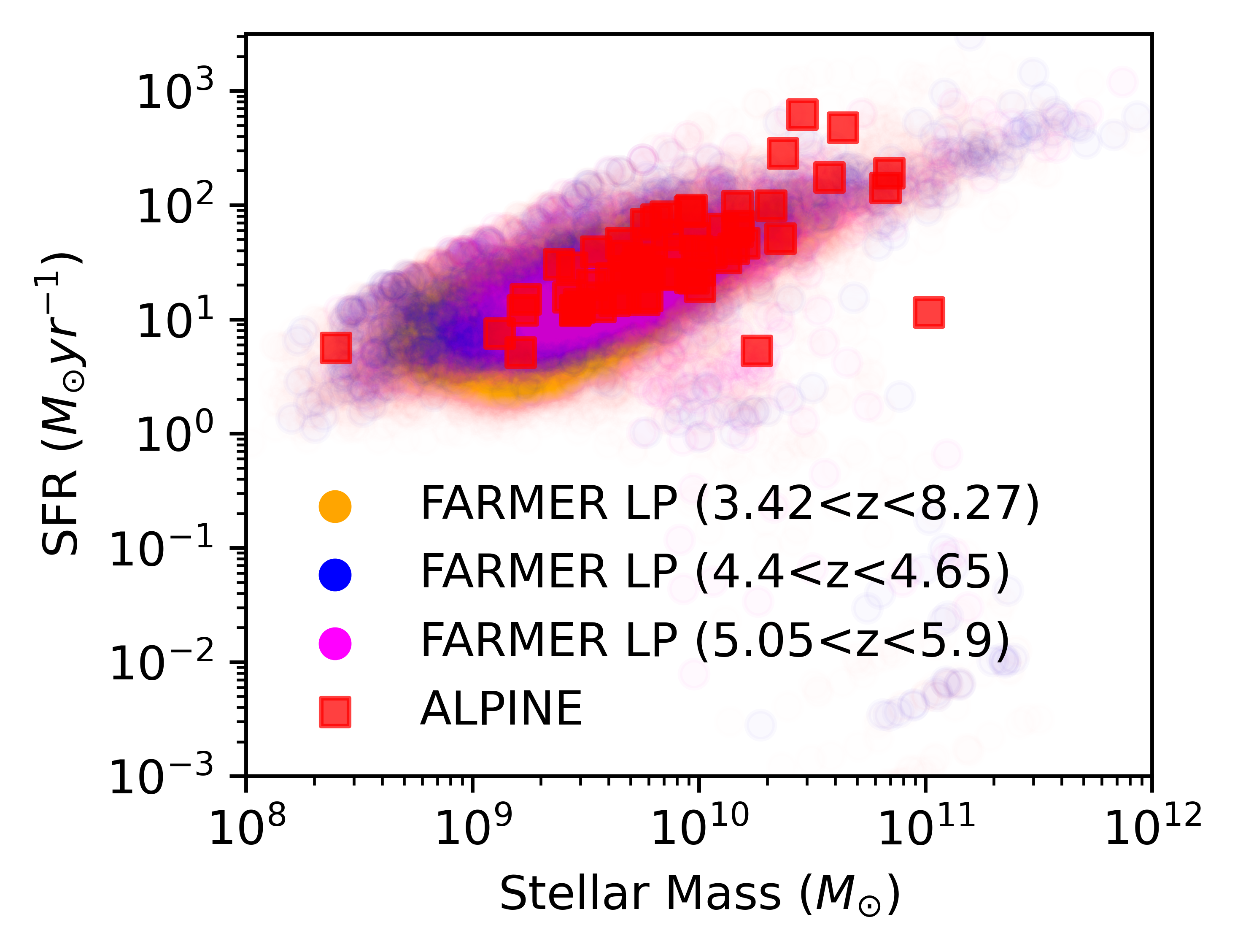
Figure 2: Distribution of galaxy SFRs and stellar masses (galaxy main sequences) for FARMER LP and ALPINE. We also take main sequences from FARMER LP in the two separate redshift bands covered by ALPINE ($4.4<z<4.65$ and $5.05<z<5.9$). The majority of ALPINE galaxies lie in this lower redshift band. All ALPINE galaxies, and most FARMER LP galaxies, lie in the galaxy main sequence area associated with SFGs (SFR $>10^{0}\,M_{\odot}\,\textrm{yr}^{-1}$ for all masses), with FARMER LP having a small number of quiescents which have low SFR and high stellar mass.

2.3 Data: COSMOS 2020

We created our intensity cubes using data from the COSMOS 2020 galaxy catalog, release version 4.1.1 (March 5, 2023, Weaver et al. 2022, 2023). These galaxies are observed in the UV through IR wavelengths, including data from GALEX, MegaCam, HST, Subaru, UltraVISTA DR4, and Spitzer. This sample is an evolution of previous work (Scoville et al. 2007; Davidzon et al. 2017) with additional inclusions from Hyper Suprime-Cam (HSC) Subaru Strategic Program (SSP) PDR2 (Aihara et al. 2019), new Visible Infrared Survey Telescope for Astronomy (VISTA) data from DR4, and additional Spitzer IRAC data. COSMOS 2020 includes $\sim$1.7 million galaxies with $z<9$ over a $1.7\times 2\deg^{2}$ area (149-151 $\deg$ right ascension (RA), 1.4-3.1 $\deg$ declination (Dec)), primarily selected using combined $izYJHK_{s}$ spectral band images. In practice this area is $1.279\deg^{2}$ (149.35-150.8 $\deg$ RA, 1.6-2.8 $\deg$ Dec) because of an outer mask region and masking of bright foreground stars, which is reduced further to $0.7\deg^{2}$ at $z>6.3$ (the area of the four Ultra-Deep stripes of UltraVISTA, McCracken et al. 2012). COSMOS 2020 is organized in two separate samples: CLASSIC, which was created using Source Extractor and IRACLEAN (Laigle et al. 2016), and THE FARMER, which was created using The Tractor photometry code (Lang et al. 2016). Photometric properties were computed for each sample using LePhare (Arnouts et al. 2002) and EAZY (Brammer et al. 2008), leading to four sub-samples with different galaxy measurements and properties. As Weaver et al. (2023) use THE FARMER with the LePhare photometric code, we adopt that sub-sample and refer to it as FARMER LP, using this term synonymously with the galaxy catalog data from COSMOS 2020.

From FARMER LP, we took galaxies with photometric redshifts within a square area ($1.2\times 1.2\deg^{2}$, 149.6-150.8 $\deg$ RA, 1.6-1.8 $\deg$ Dec) in the redshift ranges described in Sect. 2.1, $3.42<z<3.87$, $4.14<z<4.76$, $5.34<z<6.31$, and $6.75<z<8.27$. Weaver et al. (2023) removed galaxies with IRAC Channel 1 AB magnitudes above 26 as these galaxies are likely to be artifacts, and when we did the same we obtained 14 611, 9322, 1732, 510 galaxies respectively. We took LP_zPDF as photometric redshift, MASS_MED for stellar mass, SFR_MED for SFR, sSFR_MED for specific star formation rate (sSFR), and IRAC_CH1 for Infrared Array Camera (IRAC) channel 1 magnitudes from the Spitzer Space Telescope.

Weaver et al. (2022) noted that COSMOS 2020 is increasingly incomplete at high redshift because they were not able to select galaxies by mass above $z>3.5$, due to a lack of $K_{s}$ band detections. Correspondingly we expect to miss many low-mass galaxies in the redshift ranges we cover, with their 75% mass completeness limit for $z=3.5$ being $10^{9.3}M_{\odot}$. The ramifications of this are discussed extensively in Sect. 4. We also expect to miss many quiescent galaxies in FARMER LP (Weaver, priv. comm). However there is little evidence that they provide a significant fraction of the total [CII] emission at any redshift, as their [CII] emission is dominated by diffuse regions instead of PDRs (e.g. Pierini et al. 1999; Boselli et al. 2002). In addition, evidence from the local universe shows that most massive quiescent galaxies have $L_{[\textrm{CII}]}<10^{7}\,L_{\odot}$ (e.g. Pineda et al. 2018; Temi et al. 2022), several dex below typical SFGs. Therefore, this quiescent galaxy incompleteness is unlikely to be a significant source of uncertainty for us.

2.4 [CII] modelling

When creating mock LIM cubes we used several [CII] luminosity relations from the literature as well as relations derived from ALPINE, which are applied to FARMER LP. While applying one model to all categories of galaxies is overly simplistic and fails to account for the nuances between different galaxy types, using a wide range of models should cover many potential scenarios including dependencies on different bulk properties. We took models from previous literature that used empirical data instead of those that used PDR modelling and other simulations, in order to reduce the number of assumptions made when creating our intensity cubes and power spectra. We also excluded models that were based on data that are irrelevant to our sample, such as models based solely on dwarf galaxies. All models assume a linear correlation in log-log space between [CII] and SFR as described in Eq. 1, with fit parameters in Table 1.

$$\log_{10}\left(\frac{L_{[\textrm{CII}]}}{L_{\odot}}\right)=a+b\log_{10}\left(\frac{\textrm{SFR}}{M_{\odot}\textrm{yr}^{-1}}\right)$$ (1)

• De Looze et al. (2014): The authors determine linear log-log relations and the scatter between SFR and IR line emission from dwarf galaxies in the Herschel Dwarf Galaxy Survey (Madden et al. 2013). By using IR-[CII] proportionalities the authors then find linear log-log [CII]-SFR models, which are calculated separately for individual populations. We only took the relations involving the entire sample or only starburst galaxies, as the other fits are specifically for small dwarf galaxies which would be inappropriate to apply to the SFG-dominated FARMER LP. We refer to these models as DL14 Entire and Starburst.

• Silva et al. (2015): The authors use a number of [CII] relations derived from high-redshift and local galaxies, as well as a SFR-$L_{\textrm{IR}}$-$L_{\textrm{FIR}}$-$L_{[\textrm{CII}]}$ relation that assumes a high proportion of [CII] luminosity comes from PDRs. We took one of their models, an empirical fit to De Looze et al. (2014)’s high-redshift galaxies, as it is the most appropriate for our purposes. We refer to it as Si15.

• Schaerer et al. (2020) and Romano et al. (2022): The authors derive empirical linear log-log [CII]-SFR relations based on the ALPINE sample. Schaerer et al. (2020) fit the entire sample of ALPINE data combined with 36 other [CII] emission sources, while Romano et al. (2022) add an artificial detection based on the non-detections within the sample. While the fundamental ideas behind their model creations are the same as ours, there are several notable differences, such as how they include ALPINE data outside of the COSMOS field, and they do not find relations for properties outside of SFR. We refer to these models as Sc20 and Ro22.

Model	a	b
DL14 Entire	6.99	1.01
DL14 Starburst	7.06	1
Si15	7.2204	0.8475
Sc20	6.43	1.26
Ro22	6.76	1.14

Table 1: Linear log-log [CII]-SFR fit parameters for Eq. 1, for individual models (De Looze et al. 2014; Silva et al. 2015; Schaerer et al. 2020; Romano et al. 2022).

These models are all empirical and thus are useful for our purposes, however none of them are solely based on the ALPINE galaxies in the COSMOS field. Furthermore, as all of the models assume a [CII]-SFR relation, this results in a limited range of predictions. We also applied the models from Vallini et al. (2015) and Lagache et al. (2018) to the sample when necessary when comparing specific statistics such as the luminosity function (e.g. Fig. 8), as these models are commonly used throughout the literature.

In order to create models from ALPINE data, we fitted [CII] results to bulk property data in a similar manner to Schaerer et al. (2020) and Romano et al. (2022). However, unlike them we only used the 65 galaxies in ALPINE that lie within the COSMOS field with [CII] detections above the $3.5\,\sigma$ limit, and we attempted to fit to more variables using Eq. 2:

$$\begin{aligned} \log_{10}\left(\frac{L_{[\textrm{CII}]}}{L_{\odot}}\right)&=a+b\log_{10}(X)+c\log_{10}(Y)\\ &+d\log_{10}(X)\log_{10}(Y)\end{aligned}$$ (2)

where $a$, $b$, $c$, $d$ are the fit coefficients, and $X$ and $Y$ are bulk properties. We did attempt to fit to second-order terms, but no higher-order models successfully converged. The bulk properties we primarily used were $\textrm{SFR}/M_{\odot}\textrm{yr}^{-1}$, stellar mass $M_{\star}/M_{\odot}$ (or in the format $M_{\star}/10^{10}M_{\odot}$), but we also included specific star formation rate $\textrm{sSFR}/\,\textrm{yr}^{-1}$, and metallicity in units of oxygen abundance $Z/12+\log\textrm{(O/H)}$. We used these bulk properties due to their intrinsic links to the physical properties of the galaxy itself, and therefore $L_{[\textrm{CII}]}$ emission. While these fits cannot replicate the intricacies of gas cloud emission within the ISM of a galaxy, we believe that a wide range of simple fits that cover more conceptual space than linear log-log fits with SFR should produce a variety of different intensity cubes and corresponding power spectra. For similar reasons we attempted fits with stellar mass and sSFR even though these properties are closely related to SFR, as we aimed for the maximum amount of leeway for our fitting functions. Metallicity is not included in the ALPINE sample data, but we calculated it for each galaxy using Mannucci et al. (2010)’s method (Eq. 3):

$$\log_{10}\left(\frac{Z}{12+\log\textrm{(O/H)}}\right)=8.90+0.37\log_{10}\left(\frac{M_{\star}}{10^{10}M_{\odot}}\right)\\ -0.14\log_{10}\left(\frac{\textrm{SFR}}{M_{\odot}\textrm{yr}^{-1}}\right)-0.19\log^{2}_{10}\left(\frac{M_{\star}}{10^{10}M_{\odot}}\right)\\ -0.054\log^{2}_{10}\left(\frac{\textrm{SFR}}{M_{\odot}\textrm{yr}^{-1}}\right)+0.12\log_{10}\left(\frac{M_{\star}}{10^{10}M_{\odot}}\right)\log_{10}\left(\frac{\textrm{SFR}}{M_{\odot}\textrm{yr}^{-1}}\right)$$ (3)

We did not attempt to fit models with spectral lines (such as [OIII]), IR emission, or redshift, as these properties do not directly affect the physical environment that results in the [CII] emission. In this way, we only used [CII] models relating to the physical bulk properties of the galaxies.

We applied these fits to all 65 data points using standard least-squared fitting procedures, as well as to these data points sorted into 5 bins. We attempted to bin by each bulk property. As we performed this procedure for all combinations of bulk properties, we retrieved a large number of potential models. However, most of these models had poor fits or did not make physical sense, so we applied procedures to find the best models as described in Appendix A. This resulted in four best-fit models within the $4\,\sigma$ limit, shown in Eqs. 4 through 7. We calculated errors in the fit parameters using Monte Carlo methods.

$$\begin{aligned} \log_{10}\left(\frac{L_{[\textrm{CII}]}}{L_{\odot}}\right)&=48.22(\pm 12.07)-3.49(\pm 2.24)\log_{10}\left(\frac{M_{\star}}{M_{\odot}}\right)\\ &-5.616(\pm 1.417)\log_{10}\left(\frac{Z}{12+\log\textrm{(O/H)}}\right)\\ &+0.508(\pm 0.220)\log_{10}\left(\frac{M_{\star}}{M_{\odot}}\right)\log_{10}\left(\frac{Z}{12+\log\textrm{(O/H)}}\right)\end{aligned}$$ (4)

$$\log_{10}\left(\frac{L_{[\textrm{CII}]}}{L_{\odot}}\right) =4.02(\pm 0.35)+0.476(\pm 0.035)\log_{10}\left(\frac{M_{\star}}{M_{\odot}}\right)$$ (5)

$$\begin{aligned} \log_{10}\left(\frac{L_{[\textrm{CII}]}}{L_{\odot}}\right)&=3.31(\pm 0.38)-0.33(\pm 0.16)\log_{10}\left(\frac{\textrm{SFR}}{M_{\odot}\textrm{yr}^{-1}}\right)\\ &+0.601(\pm 0.057)\log_{10}\left(\frac{M_{\star}}{M_{\odot}}\right)\end{aligned}$$ (6)

$$\begin{aligned} \log_{10}\left(\frac{L_{[\textrm{CII}]}}{L_{\odot}}\right)&=6.14(\pm 1.29)-0.31(\pm 0.15)\log_{10}\left(\frac{\textrm{sSFR}}{\textrm{yr}^{-1}}\right)\\ &+0.27(\pm 0.12)\log_{10}\left(\frac{M_{\star}}{10^{10}M_{\odot}}\right)\end{aligned}$$ (7)

These models are m1-m4 respectively. They show a greater variety of behaviour compared to the linear log-log [CII]-SFR models of the previous literature: m1 has a high level of complexity with cross terms in metallicity, m2 is a simplistic model with regards to stellar mass instead of SFR, and m3 and m4 have terms based on stellar mass and SFR. Despite these differences in construction and complexity, the resulting galaxy [CII] luminosities were relatively similar: when applied to any given galaxy, the [CII] luminosities always lay within 1 dex. It initially seemed surprising that none of these models are solely based on SFR, in contrast to previous literature. However, we still retain this core conceptual relation because there is a close correlation between SFR and stellar mass for SFGs, as shown in the galaxy main sequences of ALPINE and COSMOS 2020 (Fig. 2).

We note that m1-m4 are likely to be more applicable to redshift bands $4.14<z<4.76$ and $5.34<z<6.31$, as the galaxy distribution of ALPINE is more representative of COSMOS 2020 at these redshifts. Consequently we treated results at $3.42<z<3.87$ and $6.75<z<8.27$ with caution, as discussed in Sect. 5.

In conclusion, we took DL14, Si15, Sc20, and Ro22 from the previous literature (Eq. 1 with Table 1), and obtained m1-m4 from the ALPINE sample (Eqs. 4, 5, 6, 7). We group models together in upcoming figures to aid readability (Figs. 7, 10, 11, 15, 16, 17), typically using purple for DL14, Si15, Sc20, and Ro22, blue for m1-m4, orange for all models with no extrapolation, and red when using mass function extrapolation.

2.5 Map creation

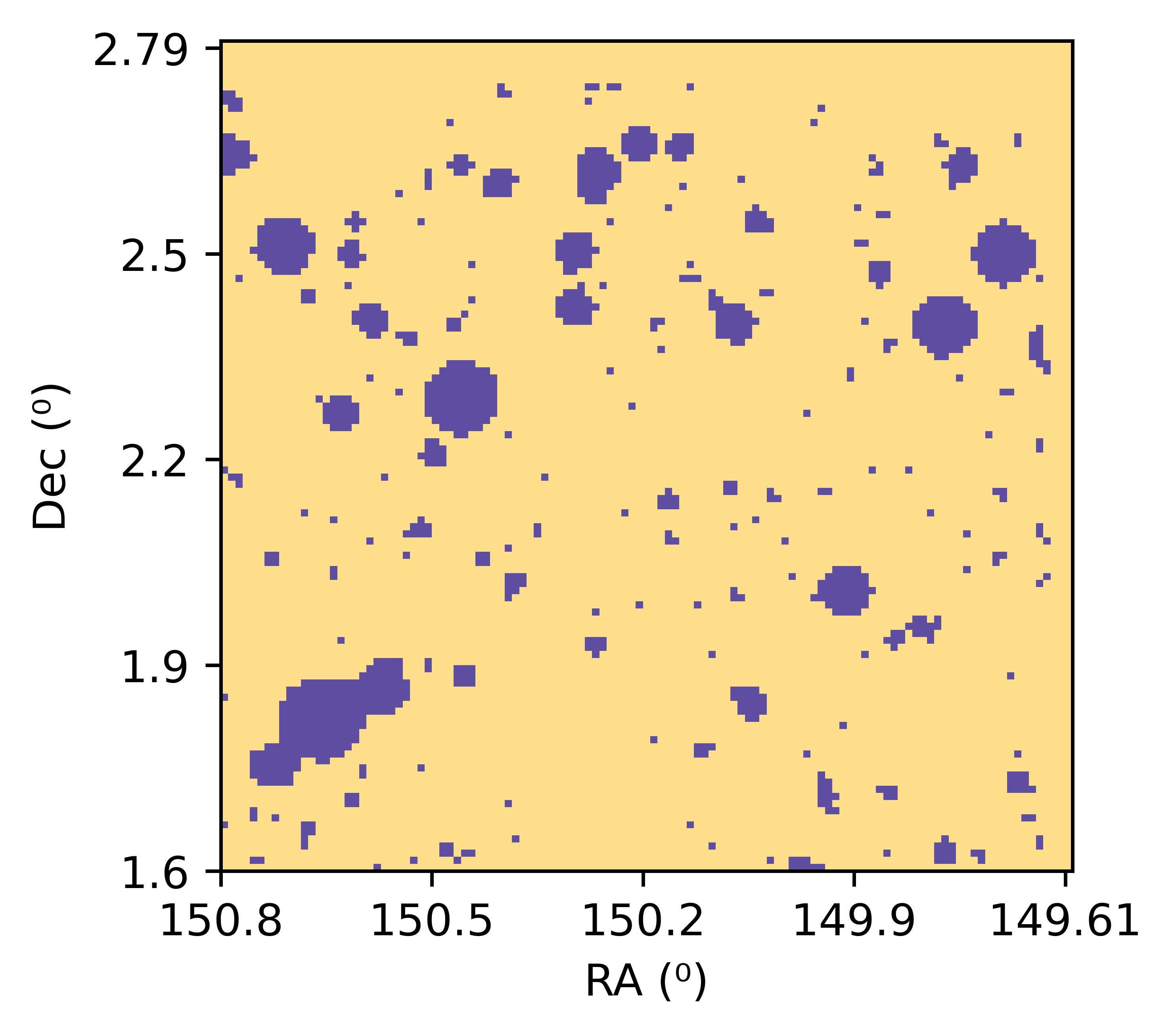
Figure 3: Map of the area covered by COSMOS 2020 over $3.42<z<8.27$. The regions masked due to foreground stars are shown in blue.

When making our mock LIM cubes, we covered a $1.2\times 1.2\deg^{2}$ area corresponding to 149.6–150.8 $\deg$ RA and 1.6–2.8 $\deg$ Dec, and an appropriate 40 GHz wide frequency band. We determined the dimensions of the cube using the EoR-Spec specifications (Nikola et al. 2022, 2023) and the data in the COSMOS 2020 catalog paper (Weaver et al. 2022). In our cube, equivalent to a 3D array, each voxel has the dimensions relating to the angular and spectral resolution of EoR-Spec as discussed in Sect. 2.1 ($37.2\arcsec$, $39\arcsec$, $46.2\arcsec$, $52.8\arcsec$ and 4.1, 3.5, 2.8, 2.2 GHz for $3.42<z<3.87$, $4.14<z<4.76$, $5.34<z<6.31$, $6.75<z<8.27$ respectively). Using the $1.2\times 1.2\deg^{2}$ square area this results in cube dimensions of $117\times 117\times 10$, $112\times 112\times 11$, $94\times 94\times 14$, and $82\times 82\times 18$ voxels respectively. This third ‘depth’ dimension, despite covering far fewer voxels, spans a larger comoving distance than is covered by the 2D sky map, so this ‘cube’ is actually a cuboid.

In these 3D cubes we inserted each galaxy’s luminosity at the corresponding voxel location, depending on its RA, Dec, and luminosity distance, calculating luminosity distances using the redshift and the cosmology in Sect. 1. We only include galaxies with photometric redshifts corresponding to the relevant channels, and make sure to convert the galaxy co-ordinate data in FARMER LP to fit this new co-ordinate scheme, accounting for the outer mask surrounding COSMOS 2020 and the FARMER LP catalog pixel size of $0.15\arcsec$. However, when creating the mock cubes, we found that the width of the spectral bins is narrower than the uncertainty in photometric redshift for many FARMER LP galaxies (typically $\Delta z\approx$ 0.1). This redshift scatter implies that galaxies from the sample could potentially be in different frequency slices of the intensity cube, which has implications for the structure of the mock cubes and therefore the resulting power spectrum. Upon investigation we found that the difference in power spectra magnitude from this scatter is less than 0.1 dex, as discussed in Appendix B. We note that this is an issue for our technique of constructing mock cubes and our results, and this will not be a problem for the actual instrument.

As we need intensity cubes, we used Eq. 8 to determine intensity ($I_{[\textrm{CII}]}$) from [CII] luminosity:

$$\frac{I_{[\textrm{CII}]}}{L_{\odot}/\textrm{Mpc}^{2}/\textrm{GHz}/\textrm{rad}^{2}}=\frac{\textrm{rad}^{2}}{\Delta\theta_{\textrm{beam}}^{2}}\sum_{i}\frac{\textrm{GHz}}{\Delta\nu_{0}}\frac{L_{[\textrm{CII}],i}}{L_{\odot}}\frac{\textrm{Mpc}^{2}}{4\pi r_{i}^{2}(1+z_{i})^{2}}$$ (8)

where $L_{[\textrm{CII}]}$ is the luminosity of each galaxy in the voxel (referred to by index $i$), $\Delta\nu_{0}$ is the frequency channel of a given redshift slice in the 3D data cube, $r(1+z)$ is the luminosity distance because $r$ is comoving distance and $z$ is redshift, and $\Delta\theta_{\textrm{beam}}$ is the instrument beam width (specifically the full width half maximum), which is equivalent to the angular size of the voxel on the sky. We then converted these units to $\textrm{Jy\,sr}^{-1}$, which are our preferred units by convention.

After performing this for the original FARMER LP sample, we then accounted for masked regions of COSMOS 2020 due to foreground stars, the ‘stellar mask’. This removal of unwanted signal creates areas of no intensity, as shown in Fig. 3. As these regions span over an total area of $0.12\deg^{2}$, approximately 10% of the area of FARMER LP, this could potentially impact the power spectra. The statistical averaging would be skewed by the voids, thereby resulting in an increase of power spectra magnitude by approximately 10%, and compensating for the changed volume could add additional complications. We used extrapolation to counteract this: the process of adding mock galaxy data to FARMER LP sample based on projected incompleteness of the original sample. In the case of mask extrapolation, we added a number of galaxies to the sample in the masked regions to ensure the galaxy density of masked and unmasked regions was made equal, that is $\sim$10% of the number of galaxies in original sample. For example, for the 14 611 galaxies in the $3.42<z<3.87$ region, we would add 1 964 galaxies. The locations were randomly picked within the voids, and the properties of the galaxies were randomly selected from the existing galaxies in the redshift band, which on average reproduced the existing luminosity function and galaxy distribution of the sample. In this way we do not expect the [CII] luminosity function, as shown in Fig. 8, to be meaningfully affected by this extrapolation. To ensure we reproduce these existing statistics in these extrapolated data, we created 10 random masks to use in intensity cube creation, and averaged the resulting power spectra of these cubes. We discuss this further in Appendix B, where we demonstrated that these corrections are appropriate. An example of an extrapolated intensity cube is shown in Fig. 4.

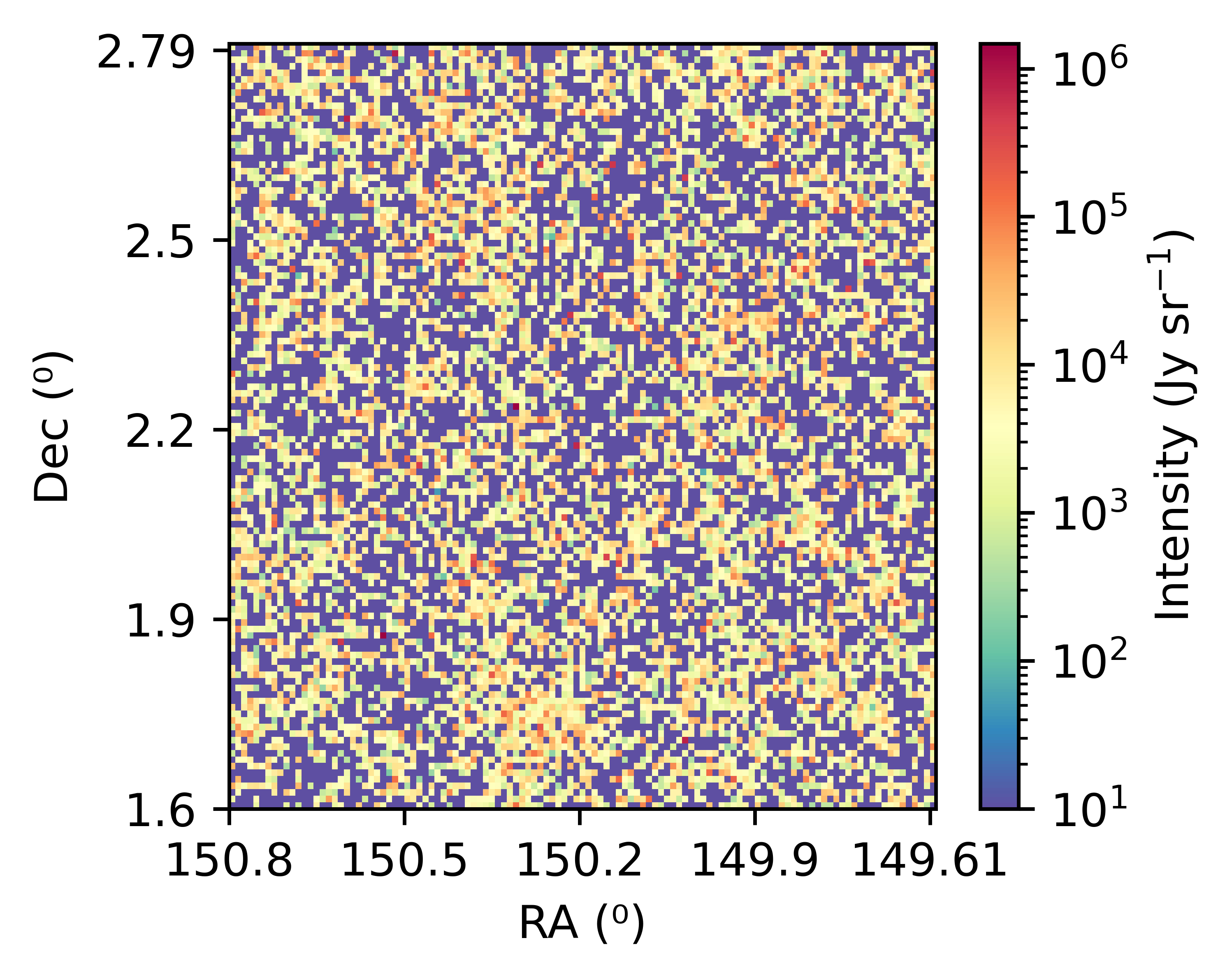
Figure 4: 2D cross-section of the 3D intensity cube at $3.42<z<3.87$, having applied m1 to FARMER LP. The mask indicated by Fig. 3 has been filled with extrapolated galaxies.

For $z>6.3$ most galaxy data are concentrated in the $0.7\deg^{2}$ covered by the four Ultra-Deep stripes of UltraVISTA (McCracken et al. 2012), the areas defined by Weaver et al. (2022). We therefore applied our mask extrapolation methods to the regions not covered by the stripes for the band $6.75<z<8.27$, as shown in Fig. 5. This mask extrapolation approximately doubled the FARMER LP sample in that redshift range as the areas of no signal are significantly larger when compared to lower redshifts, and likely compromised any large scale structure in that band. This is discussed further in Appendix B.

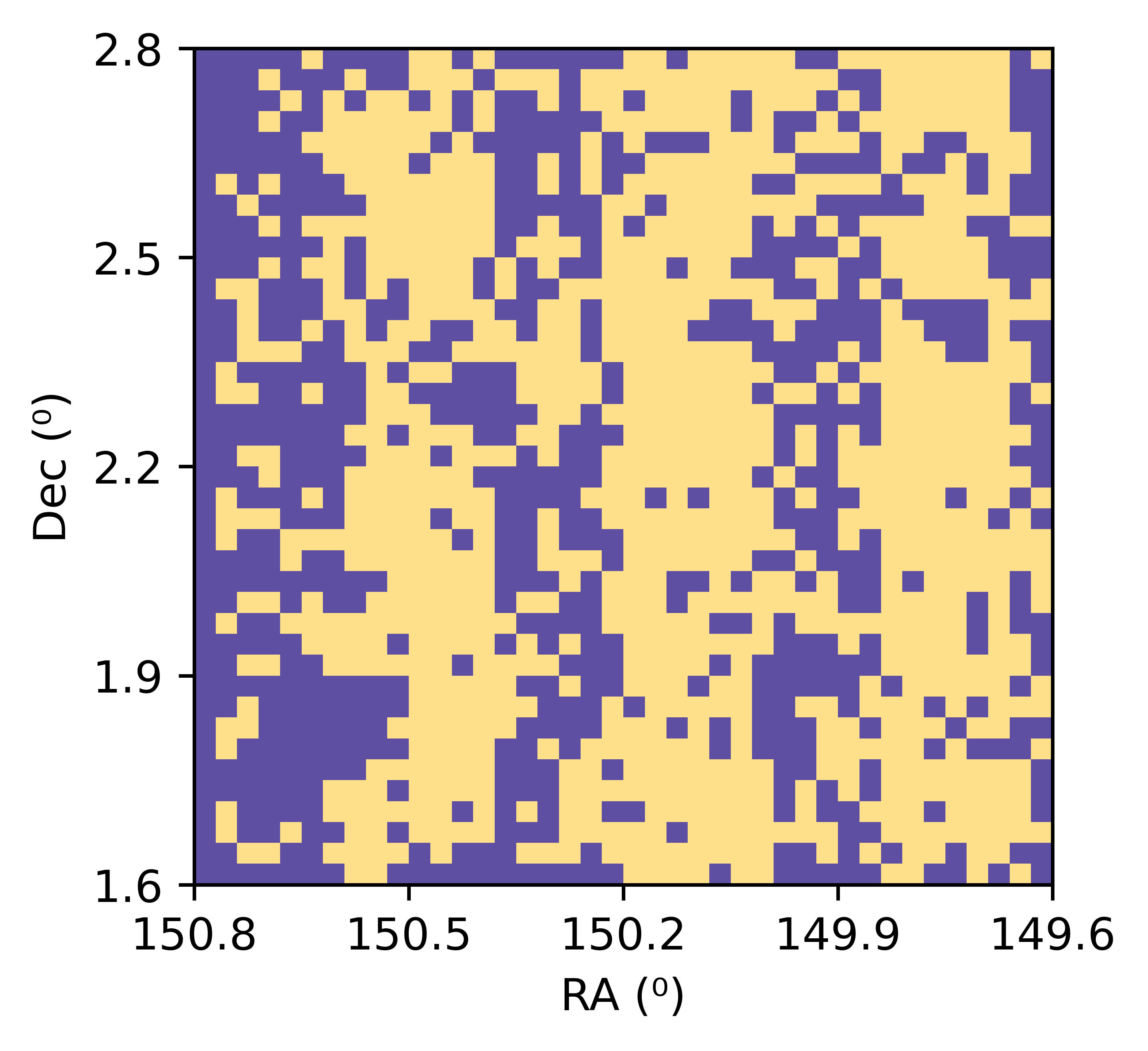
Figure 5: As Fig. 3, but only for FARMER LP galaxies with $z>6.3$. Even in the yellow stripes where we expect galaxies to be visible, there are blank pixels as we can only detect the brightest galaxies.

2.6 Power spectra

The three-dimensional spherically averaged power spectrum is the primary statistic used to analyse intensity cubes in previous work. In the context of upcoming LIM experiments, power spectra will allow us to probe the luminosity function of the covered fields and to determine the existence and impact of regions with significant galaxy clusters. This statistic is therefore useful in characterising the EoR, so we applied it to our mock intensity cubes. When performing this for maps created from mock samples, as done in this work, we already know the ‘input’ luminosity function and clustering. Therefore, the resulting power spectra can be viewed as predictions for if the real conditions match our simulated conditions.

Firstly we established the dimensions of the voxels and the intensity cube in comoving space, in units of Mpc. We then took the 3D intensity cubes and performed a Fast Fourier Transform (FFT) over all elements in the cube, producing a new 3D cube centered around the origin point in Fourier space, where each intensity element was transformed into corresponding Fourier amplitudes. These Fourier amplitudes are multiplied by the volume of a voxel divided by total number of voxels (i.e. volume of a voxel per voxel), a normalisation factor to arrive at the units of the Fourier Transform, thereby preventing the physical scale of the intensity cube from influencing the power spectra amplitude.

To get from this Fourier space cube to the power spectra $P(k)$, we had to spherically average the Fourier amplitudes for each spatial frequency bin. We determined the spatial frequency co-ordinates $k_{x}$, $k_{y}$, and $k_{z}$ corresponding to each Fourier amplitude, equivalent to $x$, $y$, $z$ in physical space. Following this we calculated the magnitude of the spatial frequency co-ordinates for each Fourier amplitude, which we refer to as $k$, using Pythagoras’ theorem. Subsequently we averaged the Fourier amplitudes of all points with $k$ co-ordinates within a given $k$ bin, of width $\Delta k$. These averaged values correspond to $P(k)$. To visualise this concept we can use Fig. 6, based on a diagram by Ponthieu et al. (2011). For our 3D cubes, we move in concentric shells of width $\Delta k$ away from the central value of $k=0$, finding the average of all values within each shell. This indicates that amplitudes corresponding to the highest $k$ values will have a greater degree of uncertainty as there will be missing $k$ modes in the cube, visualised by the green circles in the figure. The physical interpretation of these frequencies is that small $k$ represents larger physical scales, up to and including the whole intensity cube, while large $k$ represents small physical scales, including the variation of signal within individual beam widths. In the context of LIM the power spectrum at small $k$ is dominated by the impact of galaxy clusters and other large structures in ‘clustering signal’, and the power spectrum at large $k$ represents the differences between individual galaxies in ‘shot-noise signal’.

As our $k$ values are calculated by Fourier transforming the comoving length of the cube in Mpc, subdivided by the number of voxels in each dimension, $k$ is in units of Mpc^-1. Consequently, the spherically averaged power spectra $P(k)$ has units Mpc${}^{3}(\textrm{Jy\,sr}^{-1})^{2}$. By convention we multiplied $P(k)$ through to find $k^{3}P(k)/2\pi^{2}$ in units of $(\textrm{Jy\,sr}^{-1})^{2}$, and all power spectra will be shown in this format.

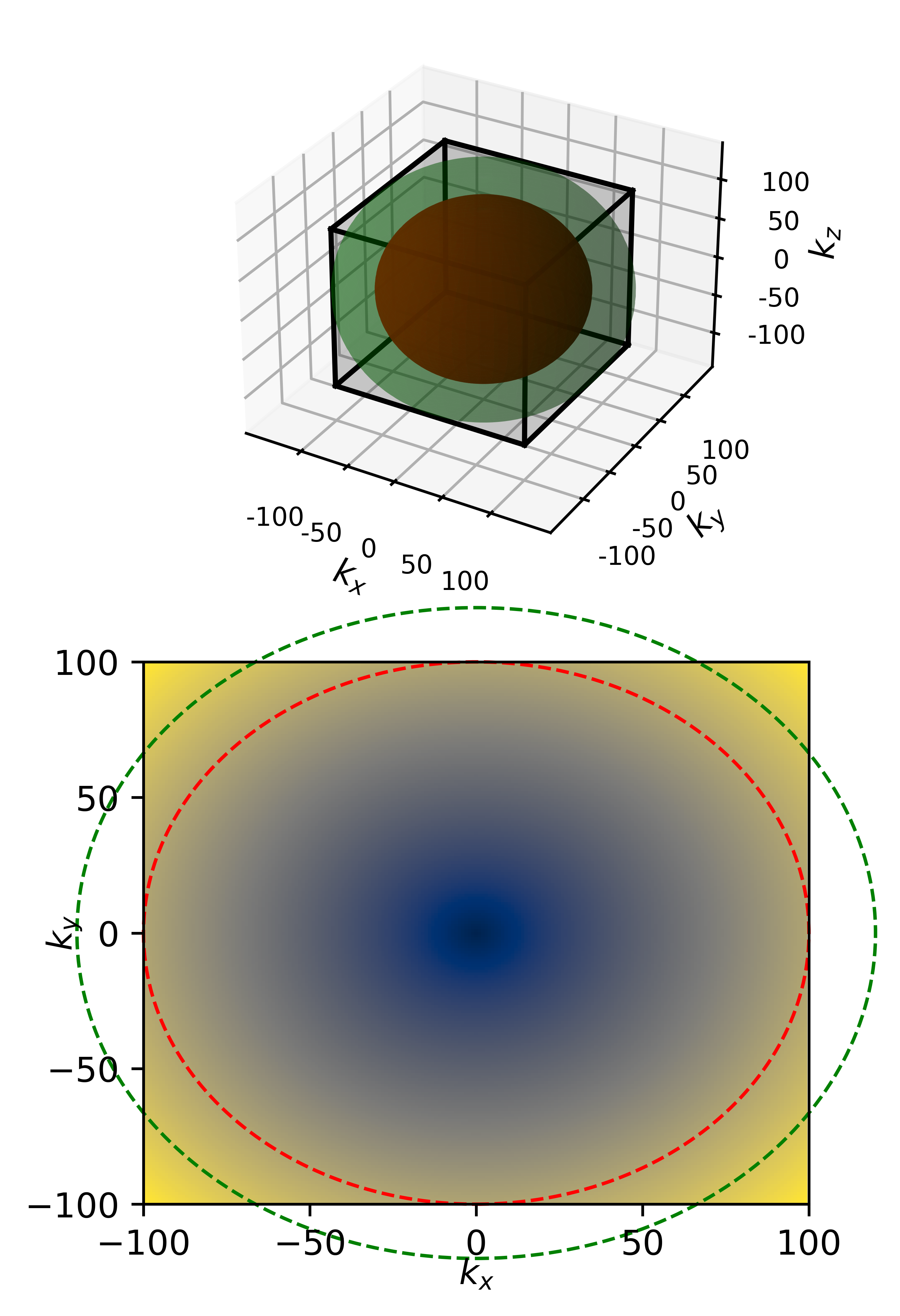
Figure 6: Fourier modes of a 3D cube and a 2D map (upper and lower subplot respectively), in the manner of Ponthieu et al. (2011). The power spectrum $P(k)$ at a given $k$ value is the average of all spatial frequencies with the same magnitude, that is concentric shells or rings around the centre where $k=0$. The inner shell or circle in red, which touches the edges of the box, is the largest $k$ value where all $k$ modes can be included. All $k$ values with higher magnitude, such as the outer shell or circle in green, lie outside the box and thus miss $k$ modes, introducing greater uncertainties in the corresponding power spectrum value. In these examples $k$ is unit-less.

Due to the size and resolution of our cubes, the $k$ scales are restricted. For a spherically averaged power spectrum the largest $k$ scale is limited by the smallest physical scale, equivalent to the comoving distance covered by one voxel on the sky map (the beam width), as discussed in detail by Karoumpis et al. (2022).

$$k_{\textrm{max}} =\frac{\pi}{r_{\perp,\textrm{min}}}$$ (9)

$$r_{\perp,\textrm{min}} =D_{\textrm{angular}}(z_{\textrm{cen}})\Delta\theta_{\textrm{beam}}$$ (10)

where $D_{\textrm{angular}}(z_{\textrm{cen}})$ is the comoving angular distance at the mean redshift of the voxel in Mpc. The smallest $k$ scale is limited by the largest physical scale, equivalent to the diagonal between two opposite corners of the intensity cube, across the distance on the sky map and the full distance covered by the redshift range:

$$k_{\textrm{min}} =\frac{2\pi}{r_{\textrm{max}}}$$ (11)

$$r_{\textrm{max}} =\sqrt{r_{\perp,\textrm{max}}^{2}+r_{\parallel,\textrm{max}}^{2}}$$ (12)

$$r_{\perp,\textrm{max}} =D_{\textrm{angular}}(z_{\textrm{cen}})\Delta\theta_{\textrm{map}}$$ (13)

$$r_{\parallel,\textrm{max}} =\frac{c}{H_{0}}\int_{z_{\textrm{min}}}^{z_{\textrm{max}}}\frac{\textrm{d}z}{\sqrt{\Omega_{\textrm{M}}(1+z)^{3}+\Omega_{\Lambda}}}$$ (14)

where $c$ is the speed of light, $\Delta\theta_{\textrm{map}}$ is the angular size of the whole sky map, $z_{\textrm{min}}$ is the low end of the redshift band, $z_{\textrm{max}}$ is the high end of the redshift band, and $\Omega_{\textrm{M}}$ and $\Omega_{\Lambda}$ are the cosmological parameters of our flat cosmology. No spatial frequencies exist outside this range.

Throughout our analysis we use two different measures to find the width of the $k$ bins, i.e. the widths of the shells. We primarily used the smallest possible interval, where there is a separate $k$ bin for each pixel in a ring around the origin in the 2D plane. This corresponds to using half the number of pixels along the map dimension$+1$ (60, 57, 50, 42 for $3.42<z<3.87$, $4.14<z<4.76$, $5.34<z<6.31$, $6.75<z<8.27$ respectively) giving a frequency width between $k$ modes of $\Delta k=0.043,0.040,0.037,0.035$ Mpc^-1 respectively. The second method used far larger $k$ bins with $\Delta k=0.3$ Mpc^-1, similar to those used in preliminary LIM work such as Chung (2022). All power spectra in future figures will use narrower bins unless stated otherwise, due to their increased frequency resolution.

We also determined a first estimate of the error in our power spectra in order to find the S/N. This error, $\sigma$, depends on instrumental thermal noise, the sample variance from binning $k$ modes, and instrumental beam smoothing. It was formulated by Li et al. (2016), and we followed the adapted version of their process as used by Chung et al. (2020) and Karoumpis et al. (2022). The full details of its calculation is shown in Appendix C, with the most important takeaway being that $\sigma$ is inversely proportional to bin size. Correspondingly power spectra with narrower $k$ bins have greater relative errors.

3 Results

We now discuss the sample of empirical data, and the power spectra resulting from the generated 3D intensity cubes, comparing our models to each other and to previous simulated work. Due to the incompleteness of FARMER LP, the range covered by our power spectra form clear lower limits, the minimum estimate for a LIM cube from observational data. By performing error analysis we also discuss the challenges in determining the power spectra for EoR-Spec in this minimum case.

3.1 Sample analysis

In order to provide appropriate context to the upcoming power spectra, we discuss the $L_{[\textrm{CII}]}$ distribution of galaxies in FARMER LP when applying [CII] models, using intensity-frequency and luminosity function diagrams. In addition, we directly compare these statistics to the samples of previous literature, primarily Yue et al. (2015), Breysse et al. (2017), Chung et al. (2020), and Karoumpis et al. (2022). We first examine the intensity-frequency (or intensity-redshift) graph and the [CII] luminosity function of FARMER LP and compare our results to those from Karoumpis et al. (2022). Here we averaged the intensity of each individual slice within the intensity cubes, equivalent to each individual frequency channel within the 40 GHz bands, and plotted against frequency or redshift. We did this for all models applied to the FARMER LP galaxies for the frequency channels covered by our cubes.

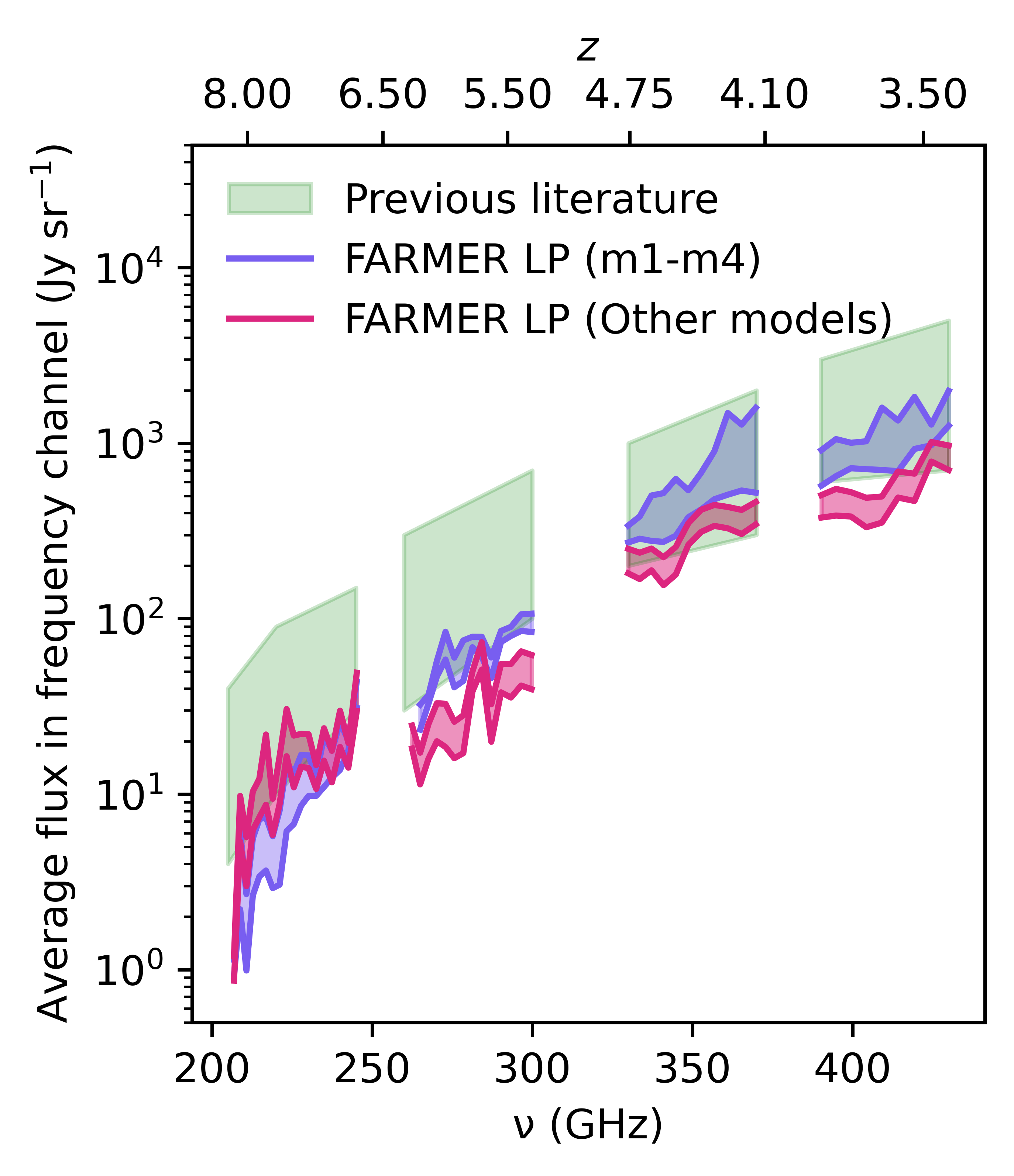
Figure 7: Average [CII] intensity of slices of the 3D intensity cubes (in units of Jy sr^-1), plotted against the frequencies and redshifts of the respective slices. We separate the results from our cubes into the models from ALPINE and the models from the previous literature, in blue and purple respectively. We compared the results of our cubes to the equivalent statistic from previous simulated cubes in green (all taken from Karoumpis et al. 2022, including itself and Yue et al. 2015; Breysse et al. 2017; Chung et al. 2020).

We only performed this analysis for the 40 GHz frequency bands we cover to maintain consistency with other works, as well as to not misleadingly cover frequencies where there is low transmission through the atmosphere. Figure 7 shows that the previous literature is broadly in agreement with itself, within 1 dex, and demonstrates the expected result: low mean intensity at low frequency, which rises with frequency in a curve shaped similarly to a logarithm. Their results follow the natural relation we expect as galaxies with the same luminosity at greater distances would give less flux, assuming [CII] emission does not significantly change with redshift. Our intensity cube channels agree with previous work at low redshift, albeit with slightly lower average intensity, indicating that FARMER LP is unlikely to be missing a significant amount of the galaxy luminosity function at lower redshift. Consequently, the significant decrease in average intensity at $5.34<z<6.31$ indicates that we have lost much of the dim end of the luminosity function at this distance. In contrast the lack of a sharp decrease at $6.75<z<8.27$ initially seems surprising in relation to the expected trend. However this behaviour is explained by the much greater mask extrapolation, drawing from a limited sample that is already biased towards the most luminous galaxies, potentially inserting more bright galaxies than we expect to exist. This indicates that our methodology is likely to be inaccurate for the $6.75<z<8.27$ band, at least when using data from the COSMOS 2020 catalog. Finally, it is shown that m1-m4 produce higher intensity slice averages when applied to FARMER LP in comparison to the previous literature models, except for $6.75<z<8.27$ (a band that ALPINE data do not cover). This potentially indicates that ALPINE’s bias towards galaxies that are further along the main sequence could produce models that overestimate [CII] intensity, which we discuss in Sect. 5.

It is important to note that it will be challenging to cleanly recover this intensity-frequency statistic from actual observations. This is because instrumental white noise and foreground signal will prevent us from accurately measuring the average [CII] intensity specifically, as discussed by Breysse et al. (2017) and Karoumpis et al. (2022). We used this statistic here as it is a clear method to compare different samples of [CII] data to each other in this idealised scenario.

We also examined the [CII] luminosity function of FARMER LP for our different redshift bands in Fig. 8, a standard measure that shows the relative density of galaxies with a given luminosity (number per unit volume per unit luminosity dex, where in this specific context dex is the magnitude interval which we take as 0.1). These luminosity functions verify that FARMER LP has a small population of [CII]-dim galaxies, because the expected Schechter curve shape (Schechter 1976) of the luminosity function falls off at $\sim$10${}^{8}L_{\odot}$ for each redshift band. For comparison, we note that the lowest [CII] luminosity from a local dwarf galaxy relevant to our work is $\sim$10${}^{4}L_{\odot}$ (Cormier et al. 2015), and that $10^{6}L_{\odot}$ is a typical [CII] luminosity of dwarf galaxies. This missing population for FARMER LP is in contrast to previous simulated work, which we show by overlaying the sample luminosity function used by Karoumpis et al. (2022) when they used Vallini et al. (2015)’s [CII] model. This demonstrates a discrepancy in sample that increases drastically below $L=10^{8}L_{\odot}$, indicating potential incompleteness in FARMER LP. However it is vital to state that we do not claim that the sample from Karoumpis et al. (2022) is more accurate than FARMER LP, but instead that simulated predictions assume greater contributions to [CII] emission from the lower end of the luminosity function. Consequently, this means that our work in the form presented in this section is useful as a scenario where the expected low luminosity galaxies do not exist, or contribute significantly less to the [CII] emission than previous simulations predict. This will be visible in the power spectrum when we make comparisons to previous simulations.

Furthermore, FARMER LP has a slightly higher proportion of high luminosity galaxies compared to some previous simulations (see $3.42<z<3.87$, $4.14<z<4.76$). For $6.75<z<8.27$, this difference exceeds 1 dex above $10^{10}L\odot$, even eclipsing FARMER LP from $5.34<z<6.31$. While the former cases are most likely due to specific simulation parameters in previous simulations, the specifics of the Vallini et al. (2015) model, or a slight sample bias towards higher luminosity galaxies in FARMER LP, the latter case is far more significant. It indicates that previous simulations vastly underestimate the number of bright galaxies at high redshift, or that there is some sample or methodological error in COSMOS 2020 for galaxies with $z>6.3$. This is also shown in our results in Fig. 7. It is possible that this is a consequence of error propagation when calculating [CII] luminosity, as shown by the error bars in the luminosity function found by Monte Carlo simulations. We discuss this further with direct comparisons to the ALMA Reionization Era Bright Emission Line Survey (REBELS, Bouwens et al. 2022) in Appendix B. While we will show results at this redshift band using this mask extrapolation to maintain consistency with the other redshift bands, we believe that results at $6.75<z<8.27$ should be viewed with caution.

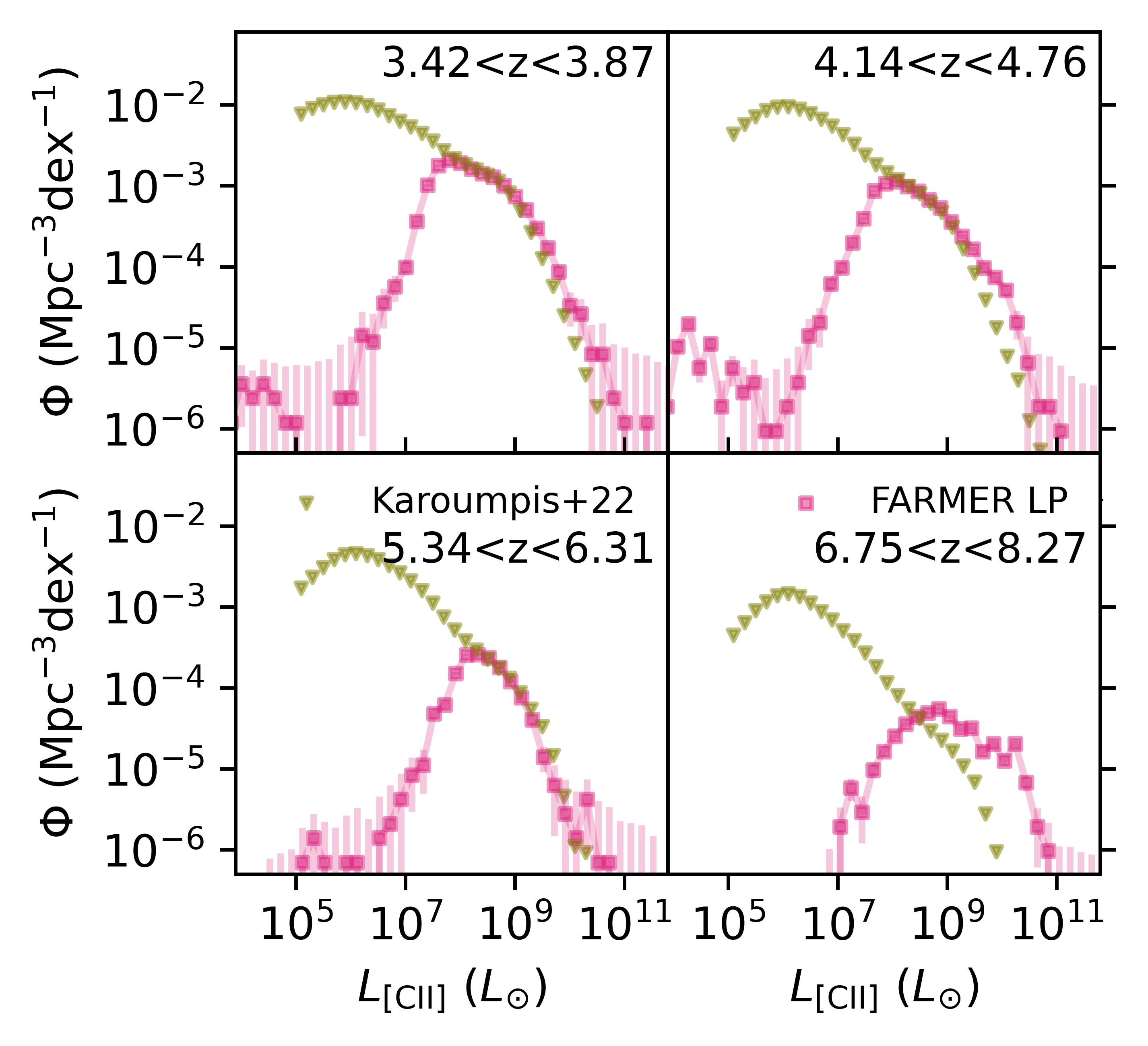
Figure 8: FARMER LP luminosity function in the four frequency bins within the range of EoR-Spec, including the extrapolated mask galaxies, shown down to $10^{4}L_{\odot}$. Comparison luminosity functions in the same redshift bands from Karoumpis et al. (2022) are also shown. As they used the [CII] model from Vallini et al. (2015), we applied the same model to ensure consistency. For all redshift bands there is a clear discrepancy below $10^{8}L_{\odot}$, as the models from Karoumpis et al. (2022) assume a significant population exists below this point, which FARMER LP does not have. At lower redshift bands, especially visible for $4.14<z<4.76$, we see small upturns in the luminosity function below $10^{6}L_{\odot}$. In addition, the luminosity function of FARMER LP shows higher populations of high-luminosity galaxies for all bands except $5.34<z<6.31$. This is most noticeable for $6.75<z<8.27$, where our function is greater by 1 dex. These deviations are likely caused or exacerbated by the propagated errors when calculating [CII] luminosity, as shown by the shaded error bars.

3.2 Power spectra, comparison to previous work, and lower limits

Our power spectra, derived from the mock samples we produced, can be viewed as predictions for if the [CII] luminosity function and clustering of the FARMER LP sample matched that of actual observations. Therefore, in the context of Figs. 7 and 8, these spectra provide lower limits for the results from EoR-Spec’s observation of E-COSMOS. Before we compare our work and the constraints they provide to the previous literature, we first show the nuances between each individual model’s power spectra for all redshift bands in Fig. 9.

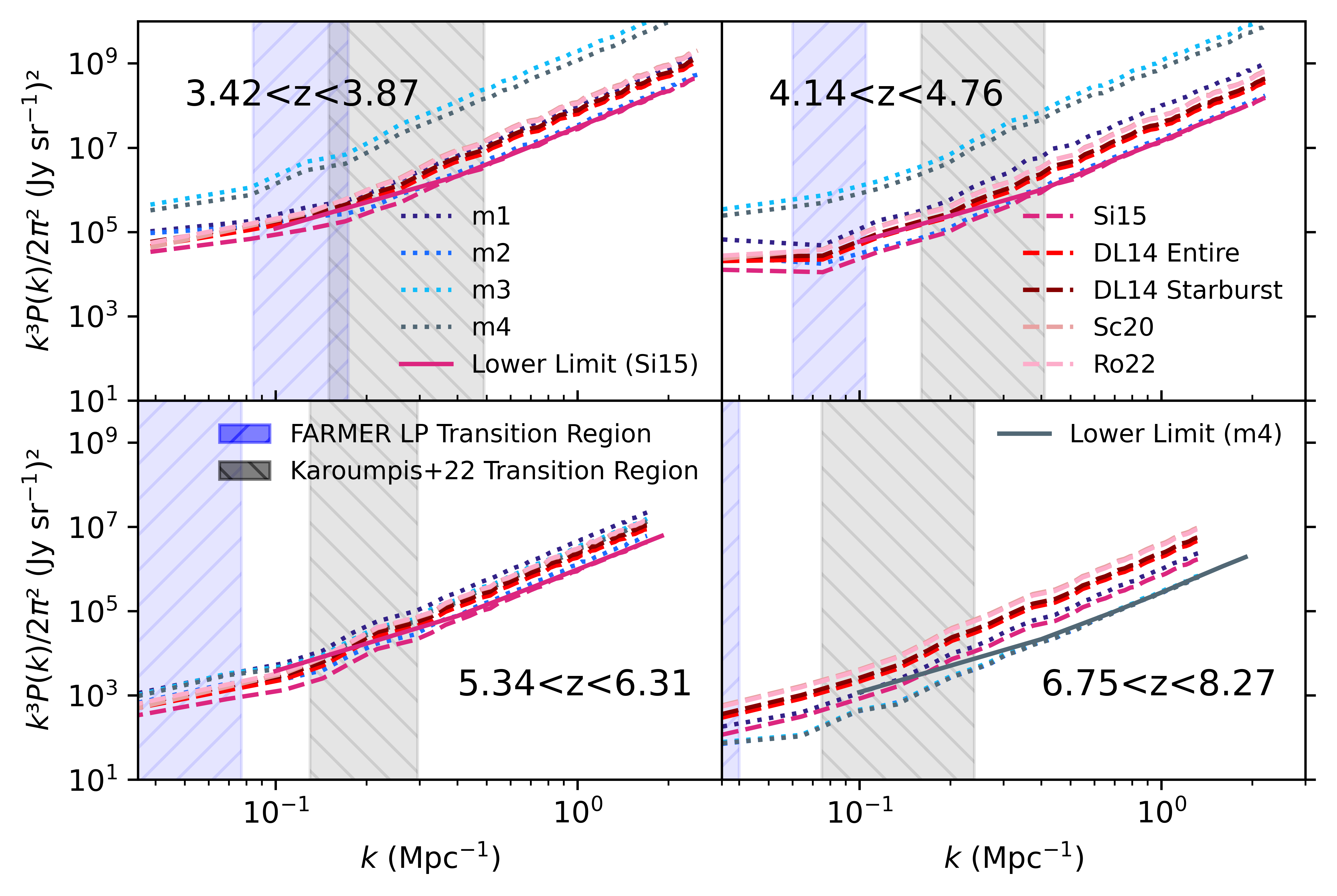
Figure 9: Power spectra of models m1-m4, Si15, DL14, Sc20 and Ro22 for all redshift bands, demonstrating a spread of up to 2 dex. We always show power spectra in the $k^{3}P(k)/2\pi^{2}$ format. Differences in maximum and minimum $k$ with regards to redshift are due to different beam and map size. The lines are kept consistent across all future graphs, however the colours change to contrast with previous simulation work. While most of these spectra are shown with smaller $k$ bins as discussed in Sect. 2.6, we also overlay the larger $k$ bin versions ($\Delta k=0.3$ Mpc^-1) of the absolute minimum power spectra (Si15 for most redshifts, m4 for $6.75<z<8.27$). These minimum values are quantified in Table 2. The upturn at lower $k$ for these lower limits is due to using wider $k$ bins compared to the other spectra. The transition region (see text) for our calculated models is shown in hatched blue, with a transition region from Karoumpis et al. (2022) shown in hatched grey for contrast.

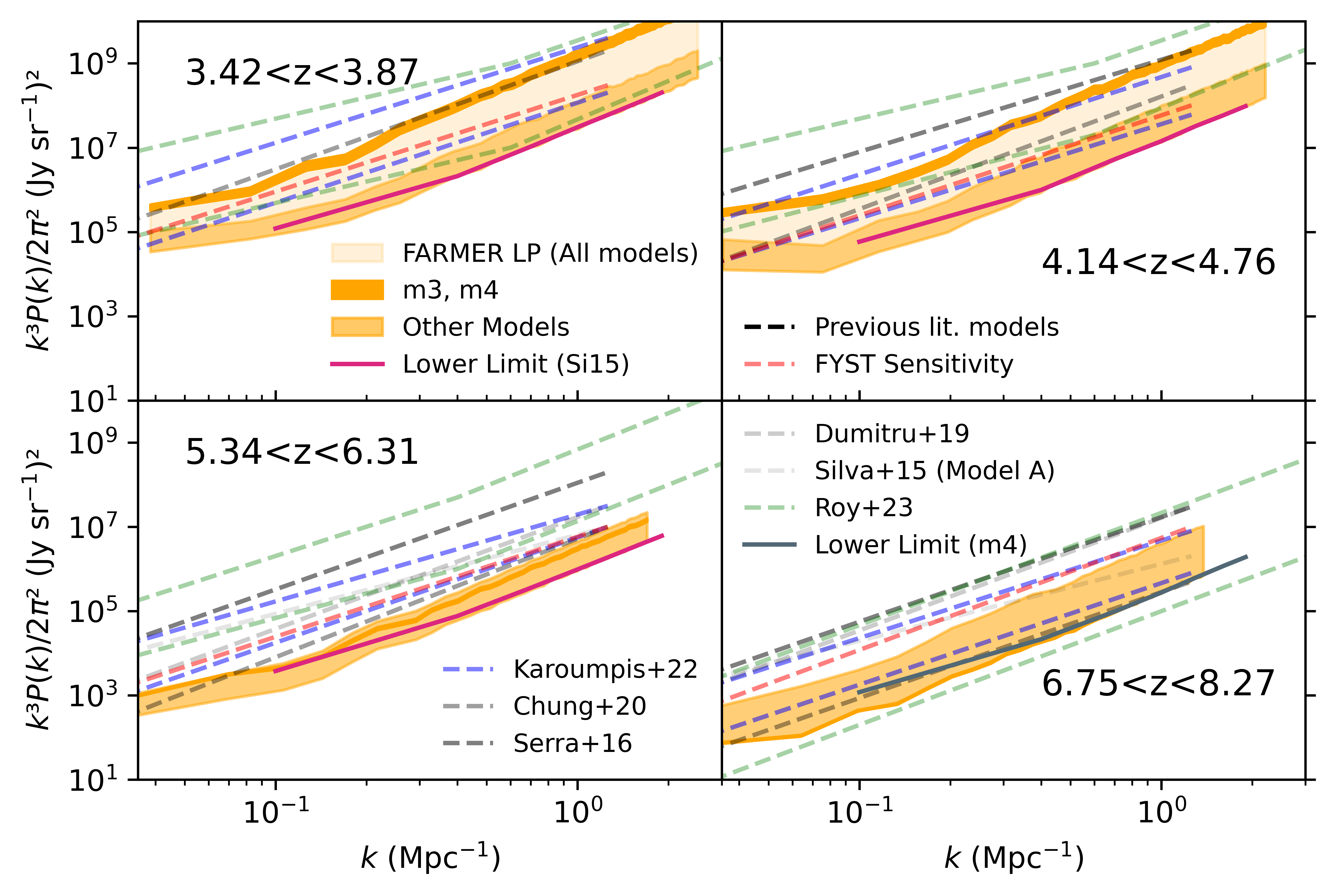
Figure 10: Power spectra at all frequency channels comparing our work to previous literature spectra. Our models are grouped together in orange, with different shadings used to highlight models m3 and m4 at $3.42<z<3.87$ and $4.14<z<4.76$. The lowest models are also shown with bin width $\Delta k=0.3$ Mpc^-1. Previous simulation work is shown with dashed lines. We also include the power spectra of the expected EoR-Spec sensitivity taken from CCAT Collaboration (2023).

We found trends amongst the magnitudes of these models, equivalent to their shot-noise and therefore their sample luminosity functions, which describe their fundamental behaviour. Overall, we see that most models (m1, Si15, DL14, Sc20, Ro22) stay within 1 dex over all redshift bands. These models, which are primarily from previous literature, exhibit the expected downward shift in magnitude with increasing redshift as intensity decreases. This trend does not continue at $6.75<z<8.27$, with the magnitudes not meaningfully decreasing due to the unusual nature of that sub-sample as discussed earlier (e.g. Fig. 7). The m2 model is similar but experiences a decrease between the final bands, which indicates that the model does not assign much intensity to the added galaxies in the large masked regions. The m3 and m4 models have significantly larger magnitudes compared to other models for $3.42<z<3.87$ and $4.14<z<4.76$, are roughly equivalent for $5.34<z<6.31$, and have significantly lower magnitudes for $6.75<z<8.27$. This could indicate that these models are influenced more by high numbers of low luminosity galaxies - that is, all galaxies give similar intensity for these models, so when FARMER LP loses faint galaxies at higher redshifts the total intensity drops, and consequently the power spectrum magnitude as well. Alternatively, this could be a consequence of ALPINE galaxies originating within $4.4<z<5.9$, as mentioned in Sect. 2.2. We also show the lowest spectra when using large $k$ bins, to visualise what observations would find in the minimum possible case. To quantify these lower limits, we show the power spectra values from Fig. 9 in Table 2.

	$k^{3}P(k)/2\pi^{2}$ ((Jy sr-1)2)
$k$ (Mpc-1)	0.25-0.55	0.55-0.85	0.85-1.15	1.15-1.45
$3.42<z<3.87$	2.11$\times 10^{6}$	1.06$\times 10^{7}$	3.06$\times 10^{7}$	6.56$\times 10^{7}$
$4.14<z<4.76$	9.93$\times 10^{5}$	5.29$\times 10^{6}$	1.43$\times 10^{7}$	3.26$\times 10^{7}$
$5.34<z<6.31$	7.66$\times 10^{4}$	3.58$\times 10^{5}$	9.80$\times 10^{5}$	2.07$\times 10^{6}$
$6.75<z<8.27$	2.16$\times 10^{4}$	9.80$\times 10^{4}$	2.77$\times 10^{5}$	6.26$\times 10^{5}$

Table 2: Lower limits of FARMER LP power spectra, where $\Delta k=0.3$ Mpc^-1. For most redshift bands this minimum model comes from Si15, with the exception of $6.75<z<8.27$ where the minimum is m4. These are also shown in Fig. 9.

Subsequently, we determined the impact of galaxy clustering on the power spectrum. As discussed in detail by Uzgil et al. (2014), the shot-noise (small scales, right hand side of each subplot) is effectively a Poisson noise effect that creates the power law shape in the $k^{3}P(k)/2\pi^{2}$ power spectra. The clustering component (large scales, left hand side of each subplot) of the power spectrum is shown by a ‘kick’ at low $k$, a deviation from the shot-noise power law. The region where both contributions are approximately equal is called the transition region, a concept we take from Karoumpis et al. (2022). We calculated this for FARMER LP (hatched blue region) by finding the $k$ modes where the magnitude of the power spectrum for each [CII] model is approximately twice that of its power law formed by the shot-noise, and then taking the median $k$ modes of these points for all the models for the given redshift band. By looking at these transition regions, we find that the kick is only noticeable at low redshifts for all models ($3.42<z<3.87$, $4.14<z<4.76$), with spectra never leaving the transition region for higher redshifts. Weaker clustering at higher redshift is similar to the work of Roy et al. (2023). Furthermore, for low-redshift bands most models exhibit kicks at $k\approx 10^{-1}\,\textrm{Mpc}^{-1}$, with notable deviations for m1 and m3. This is potentially due to m1 and m3 having low variation between galaxy [CII] emission as discussed earlier, reducing the impact of specific overdense regions.

When comparing this clustering to that of previous simulations, their spectra have far greater clustering signal, as shown by the transition region from Karoumpis et al. (2022) for their spectra in Fig. 9 (hatched grey region). This contrast is likely due to FARMER LP excluding many of the low-luminosity galaxies that surround more luminous galaxies in the sample. This therefore reduces the impact of any existing galaxy clusters on the power spectra, a problem which becomes far worse for the more-incomplete higher redshift bands. This idea can also be described by power spectra statistics as discussed by Uzgil et al. (2014) and Karoumpis et al. (2022), as lower luminosity galaxies in the sample have a significantly greater impact on the clustering signal component than the shot-noise component. In addition, as $6.75<z<8.27$ had a far larger mask (and thus more mask extrapolation), this likely resulted in most large scale structure being destroyed. Finally, when using large $k$ bins the kicks appear to occur at higher $k$, however this is an artefact due to the lower precision of these bins.

In this way, by making intensity cubes and the corresponding spectra whilst only using galaxies from COSMOS 2020, that is galaxies which we know exist without any additional signal, we derive a lower limit for possible [CII] power spectra. It is therefore unlikely that the future observed power spectra of EoR-Spec will stray below the limits as quantified in Table 2.

We then compared our power spectra to the simulated power spectra from the literature in detail, as shown in Fig. 10. In upcoming graphs we will group our power spectra together to make them more readable, with specific smaller groupings being used to examine specific models. The methodology of the previous literature is described below:

• Karoumpis et al. (2022): The authors use $4\times 4\deg^{2}$ mock scans created by the Illustris TNG300-1 simulation with frequency bands in the range covered by EoR-Spec. They assign SFR and other bulk properties to their galaxies using abundance matching. From this, the authors select a $2\times 2\deg^{2}$ region, apply models from Vallini et al. (2015), Lagache et al. (2018), and Sc20 and obtain a range of predictions. We will show these boundaries with the blue dashed lines in Fig. 10 and similar figures.

• Chung et al. (2020): The authors use the Lagache et al. (2018) model with an added scatter of $\sim$0.5 dex to emulate the deviation within said model, creating cubes from the galaxy-halo model of UNIVERSE MACHINE with EoR-Spec’s frequency bands. They acquire maps with an approximate size of $2\times 2\deg^{2}$. Their results indicate a relatively weak clustering signal, and that detection past $z\approx 6$ will be challenging.

• Serra et al. (2016): Using galaxy data from $z<4$, the authors use $L_{\textrm{IR}}$ data to infer $L_{[\textrm{CII}]}$ data assisted by a halo model. Their power spectra have a relatively high magnitude, giving an upper bound when compared to other simulations. The authors aim to cover CONCERTO (200–360 GHz) with an area of $2\deg^{2}$, which overlaps with all our bands except $3.42<z<3.87$.

• Dumitru et al. (2019): The authors use Lagache et al. (2018) without any added scatter, applied to a hydro-dynamical cosmological simulation made by the Sherwood simulation suite (Bolton et al. 2017), which is combined with the G.A.S semi-analytical model (Cousin et al. 2016) to determine SFR. They cover snapshots at high redshifts ($z\approx 6.3,7.1,8.2,9$) with an area of $1.5\times 1.5\deg^{2}$.

• Silva et al. (2015): The authors use simulations from the SImfast 2021 code (Santos et al. 2010; Silva et al. 2013) and galaxy data from De Lucia & Blaizot (2007), apply a halo mass-SFR relation, and create their cubes using their four separate [CII] models (Si15 and three others). They assume strong clustering signal and weak shot-noise, leading to a strong kick at relatively high $k$ modes. The authors cover a range of 200–300 GHz ($5.33<z<8.5$), but we only include their work at $5.34<z<6.31$ as their specific frequency bands overlap poorly with $6.75<z<8.27$. This map has a $1.35\times 1.35\deg^{2}$ coverage, similar to our work.

• Roy et al. (2023): The authors use the LIMpy package to generate power spectra with SFR provided by UNIVERSE MACHINE and Illustris TNG. The authors use a wide range of SFR models - Visbal & Loeb (2010), all models from Si15, Fonseca et al. (2017), Lagache et al. (2018), and Sc20. We show the lower and upper bounds of these models in green dashed lines. They cover the same redshift bands as us, with map sizes of $4\times 4\deg^{2}$.

As these simulated works typically cover larger sky map scales than the area covered by COSMOS 2020, their power spectra extend to lower $k$. However as power spectra are normalised with cube volume we do not expect any meaningful discrepancies in the magnitudes, and as the previous literature typically used narrow $k$ bins we expect to see the kicks to be directly comparable to our models when using narrow $k$ bins. We also show the first estimate of FYST’s sensitivity from CCAT Collaboration (2023), the approximate detection limit, for comparison purposes.

Our power spectra are almost always lower in magnitude when compared to the previous literature, including lying below the expected sensitivity of the instrument. At high $k$ most of our models partially overlap with some previous simulated work such as the lower ends of Karoumpis et al. (2022) and Roy et al. (2023). This overlap shrinks as $k$ decreases, indicating that previous work has stronger clustering components, as indicated by the transition regions in Fig. 9. While the absolute lower limits do not exclude any previous simulation work, models m3 and m4 eclipse the lower ends of other simulated models and the expected EoR-Spec sensitivity power spectrum for $3.42<z<3.87$ and $4.14<z<4.76$. However, other spectra from the literature including Serra et al. (2016), Dumitru et al. (2019), and the upper end of Roy et al. (2023) are significantly greater in magnitude than any of FARMER LP power spectra, which is to be expected as these works assume a much greater contribution from faint galaxies. $6.75<z<8.27$ is the exception to these trends with significantly greater overlap, however as noted in Sects. 2.5, 3.1 and Appendix B this band is likely limited in use.

In summary, Figs. 7 and 8 show that COSMOS 2020 provides an empirical lower limit to simulation-based estimates for the luminosity function when we apply our luminosity models. This is also demonstrated in the power spectra of Fig. 9. Our lower limits for power spectra based on existing data cannot definitively exclude the lower ends of previous simulated power spectra from the literature (Fig. 10), and the FARMER LP power spectra have comparatively weaker clustering components due to the lack of faint galaxies in the sample.

3.3 Error analysis

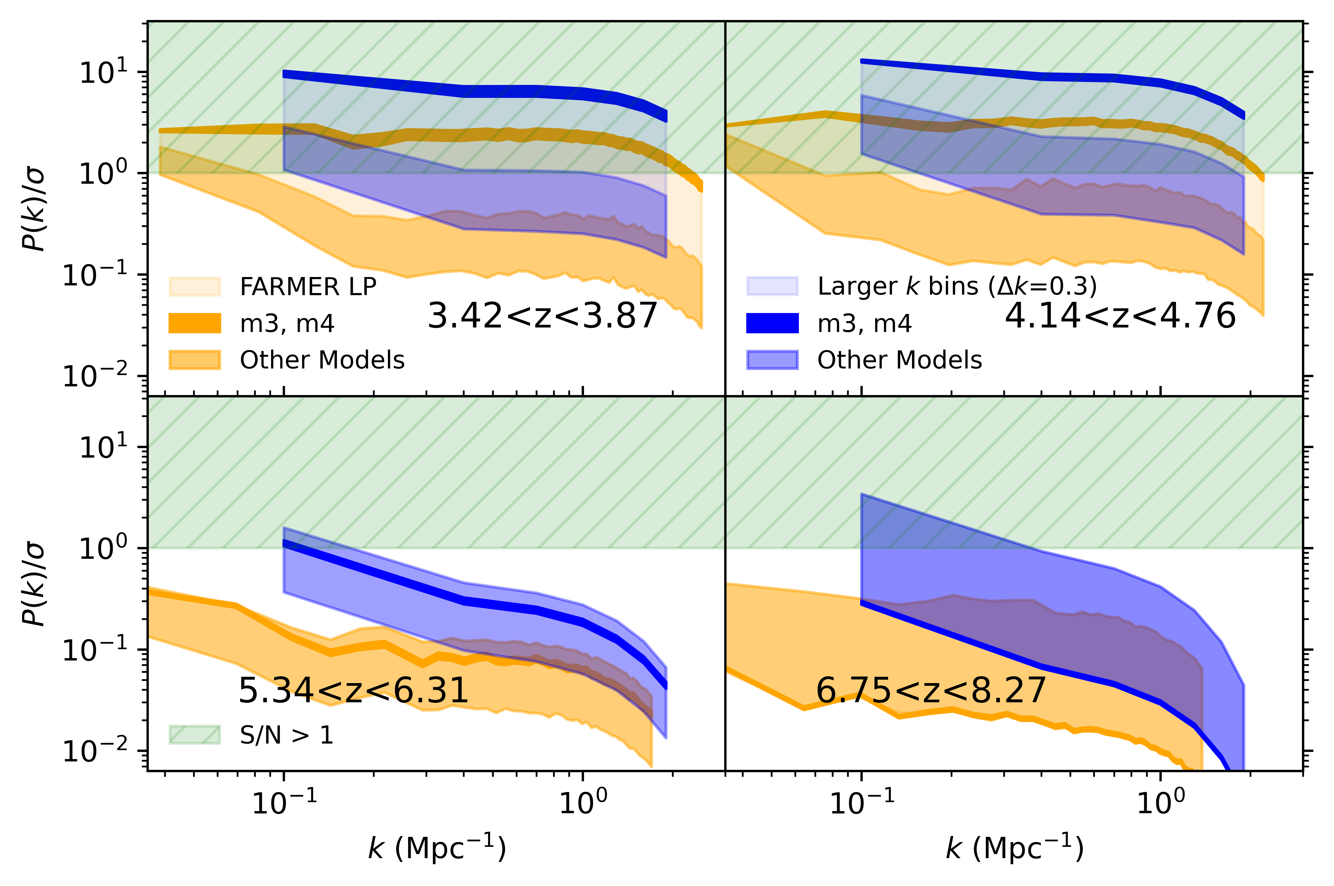
Figure 11: Comparing $P(k)$ and its error, $\sigma$, by finding their ratio (equivalent to S/N). We show the ratio of $P(k)/\sigma$ for all models and redshifts. Orange is for narrower bins of width $\Delta k=0.043,0.040,0.037,0.035$ Mpc^-1 respectively, whilst blue is for bins with width $\Delta k=0.3$ Mpc^-1. If this ratio is greater than 1, denoted by the green hatched region, we have greater signal than noise.

We find a first estimate of the error in the power spectra and visualise it in the form of the S/N $P(k)/\sigma$, where $\sigma$ is the analytically calculated instrumentation error of EoR-Spec (process described in Appendix C). While we cannot presently include all possible error contributions, such as errors from foreground contamination removal and sky noise, this does include instrumental thermal noise, the sample variance from binning $k$ modes, and instrumental beam smoothing. Measurements of $\sigma$ will be improved when we get initial data after the first light of EoR-Spec, but we consider this a good first estimate of noise in the power spectra.

When viewing the relative error for spectra in Fig. 11, we can determine useful information at $k$ scales where the S/N is above 1, that is when there is more signal than noise (denoted by the hatched green region). When using narrow $k$ bins this is possible for m3 and m4 at $3.42<z<3.87$ and $4.14<z<4.76$, but all other models fail to reach S/N$>1$ at these redshifts, and all models fail at higher redshifts. If we use wider bins we retrieve greater S/N as $\sigma$ is inversely proportional to the number of $k$ modes in a bin, a number which increases if we use wider bins (Appendix C). However, noise still dominates for lower magnitude models and models at higher redshifts. We recalculated these for greater observation time than our assumed 2000 hours, however even when using large bins, we only achieve S/N$>1$ for most models at $z<6.3$ after tripling our observation time. These calculations also assume that signal extraction is 100% efficient, so in reality these ratios are likely to be lower.

This metric indicates that observations cannot retrieve any useful information in the initial observation period for the most pessimistic cases, even when using wide $k$ bins. This issue is more pressing for shot-noise regions, which typically have greater errors compared to clustering regions, thereby leading to problems when constraining the luminosity function of observed fields. In this case higher redshift bands would be a significant technical challenge, as discussed by Chung et al. (2020).

4 Extrapolation

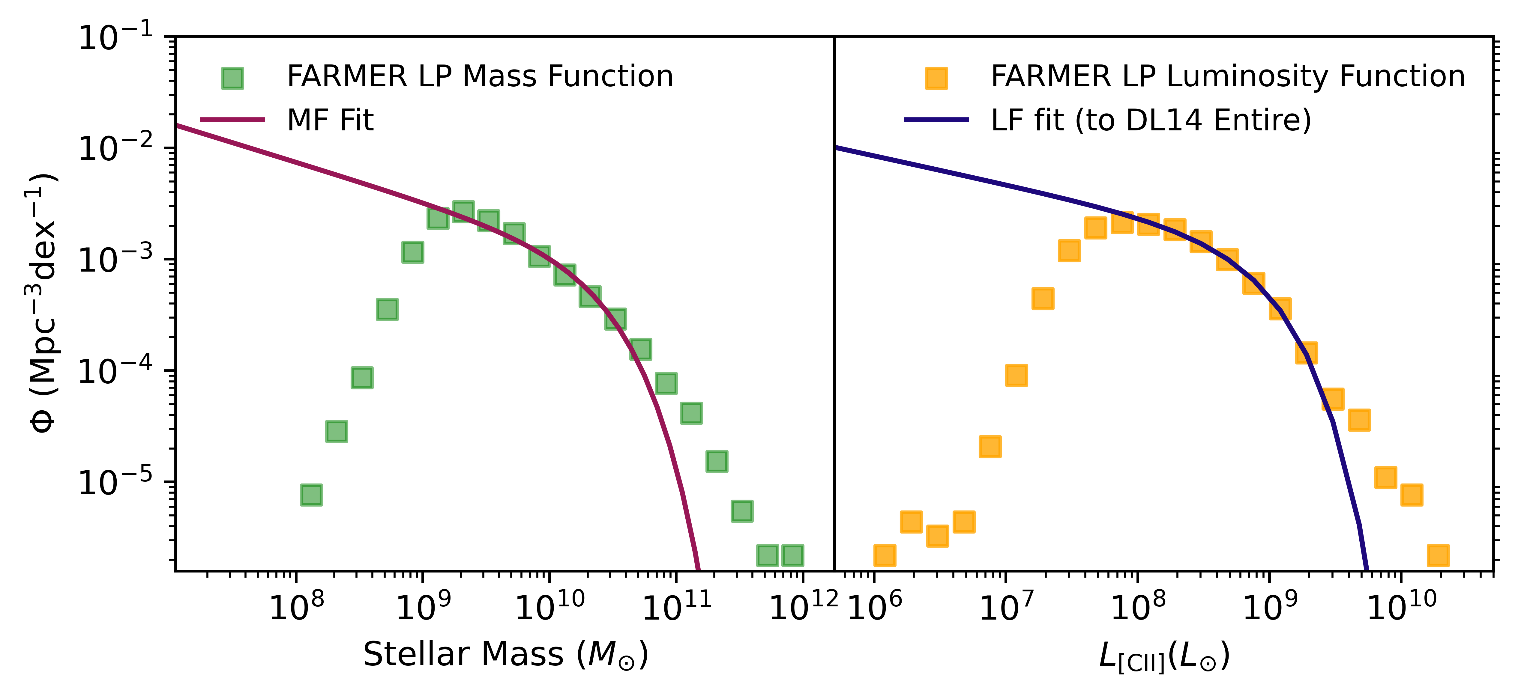
Figure 12: Examples of how Schechter fits are applied to mass functions (left) and luminosity functions (right) at $3.42<z<3.87$. The luminosity function in this case is when we apply DL14 Entire to FARMER LP. In both cases, we applied the CANDELS correction to the sample before fitting the Schechter curves. We extrapolate galaxies corresponding to the difference between the projected curves and the existing functions. While there are slight discrepancies at high mass or luminosity, this is acceptable as this extrapolation method focuses on dim galaxies, and there are higher errors for the bright end of these functions (as shown in Fig. 8).

The limited completeness of FARMER LP is useful for making our lower bound mock LIM cubes, however it is noticeably different compared to previous simulation work. This is due to their implicit assumption of fainter galaxies at high redshift contributing significantly to the [CII] luminosity function. In this context we decided to create a hypothetically more complete sample by extrapolating from FARMER LP, creating additional galaxies to fill in perceived missing gaps in the sample’s mass or luminosity function, which are then added to the mock LIM cubes. By creating a variety of spectra from physically plausible samples and checking their concordance with previous simulations, we could verify if the simulated works are consistent with existing empirical data from COSMOS 2020. In addition, as part of this extension we aimed to create reasonable upper limits for the observed power spectra, though these will not be as rigorous as the lower limits due to the inherent uncertainties in extrapolating from an existing mass or luminosity function.

When extrapolating we had to determine the number of additional galaxies with appropriate bulk properties, and devise a method to sensibly add these galaxies to the existing cubes. We explored three techniques of extrapolation: exploiting data from surveys that probed deeper than COSMOS 2020, extrapolating from the mass function of FARMER LP, and extrapolating from the luminosity functions we generated from applying [CII] models to FARMER LP. Each process was performed separately for each frequency band to account for the sample variation on different cosmological timescales. The galaxies were then added to the LIM cubes appropriately using a Voronoi Tessellation (VT) technique. After creating these samples and corresponding power spectra, we repeated our analysis with the power spectra and relative errors to show concordance with previous simulation work.

4.1 Using CANDELS data

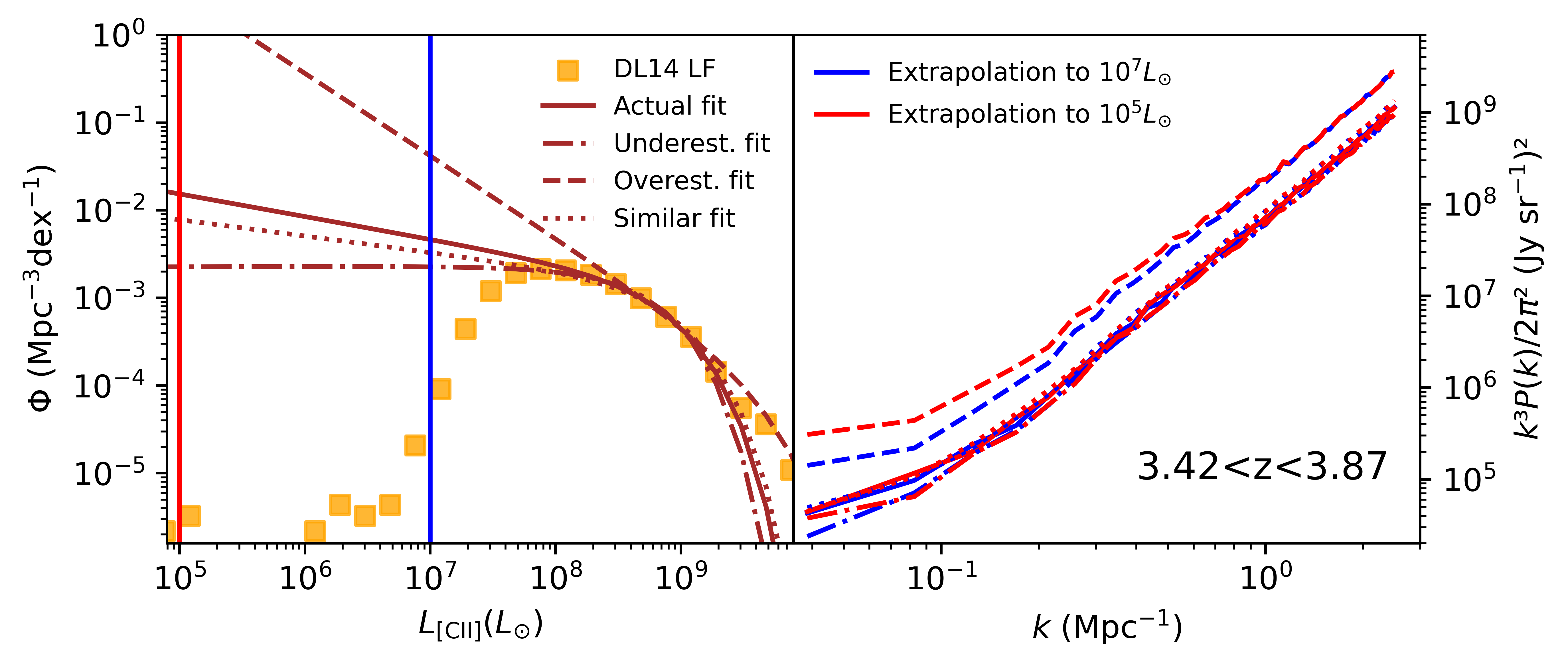
Figure 13: Comparison of different Schechter curve fits to the DL14 Entire [CII] luminosity function at $3.42<z<3.87$. This sample includes FARMER LP, the stellar mask and CANDELS factor adjustments. We include the actual fit we chose, as well as fits that are underestimates, overestimates, or were similar. Parameters for this fits are in Appendix D. The left subplot shows the actual Schechter curves themselves, including the two limits of extrapolation we investigate, and the right subplots show the resulting power spectra. The power spectra are mostly similar, except for the ‘overestimate’ case.

We made a first estimate of the incompleteness of FARMER LP by comparing it to deeper surveys in the wider COSMOS field. We primarily used the Cosmic Assembly Near-infrared Deep Extragalactic Legacy Survey (CANDELS, Nayyeri et al. 2017), which covers a $\sim$0.06$\deg^{2}$ region within one of UltraVISTA’s Ultra-Deep stripes in the COSMOS field, using HST data. Weaver et al. (2022, 2023) noted that the ratio of galaxy number in FARMER LP to CANDELS is $\sim$75% for $z>2.5$ within the region probed by CANDELS, implying that FARMER LP misses at least 25% of galaxies in that region. Therefore we planned to use the ratio between FARMER LP and CANDELS to find an appropriate number of galaxies to add to the sample. In order to do this we calculated this ratio again for each frequency band, past a certain stellar mass threshold where FARMER LP was determined to be almost ‘mass complete’ (excluding discrepancies with CANDELS). We used this mass limit as we only intended to correct for the high-mass galaxies with this method, the fainter galaxies being accounted for by Schechter curve comparisons. This mass threshold was calculated in several ways to ensure the limit was accurate, first by using the following equations from Weaver et al. (2022, 2023) for 95% mass completeness:

$$M_{\textrm{lim, `22}}=-1.51\times 10^{6}(1+z)+6.81\times 10^{7}(1+z)^{2}$$ (15)

$$M_{\textrm{lim, `23}}=-3.23\times 10^{7}(1+z)+7.83\times 10^{7}(1+z)^{2}$$ (16)

In addition we manually calculated the $M_{\textrm{lim}}$ value by following the same procedure as Weaver et al. (2023), however instead of re-scaling the 30th mass percentile of galaxies by IRAC Ch1 luminosity we took the 40th percentile of masses within FARMER LP because of our focus on high-redshift bright galaxies. All three methods return the same stellar mass thresholds within 0.05 dex, $10^{9.2}$, $10^{9.3}$, $10^{9.5}$, $10^{9.7}M_{\odot}$ for $3.42<z<3.87$, $4.14<z<4.76$, $5.34<z<6.31$, and $6.75<z<8.27$ respectively. After accounting for the stellar mask area of FARMER LP within the CANDELS region, we find the number ratio of galaxies above the mass threshold in FARMER LP to CANDELS to be 78%, 78%, 51%, and 58% respectively. We always extrapolated additional galaxies above the mass thresholds in the FARMER LP sample following these ratios before applying the other extrapolation methods. For example, for each galaxy with stellar mass above $10^{9.2}M_{\odot}$ in the $3.42<z<3.87$ sub-sample we duplicated it to generate an additional $(100/78)-1$ galaxies, or approximately 1 extra galaxy for each 4 original galaxies with mass above $10^{9.2}M_{\odot}$. In this way, this CANDELS factor corrects for the high end of the galaxy main sequence, with Schechter fits correcting for the low end.

4.2 Extrapolating from mass and luminosity functions using Schechter curves

The assumed missing dim end of the [CII] luminosity function for models applied to FARMER LP has been a key indicator of incompleteness, as shown in Fig. 8. Correspondingly, we attempted to construct more complete samples by extrapolating out from this end of the function. As a way to verify this technique we also did the same with the mass function of FARMER LP. A basic visualisation of this is shown in Fig. 12: by computing the difference between our extrapolated function and the existing function for faint galaxies within each redshift band, we can estimate the number of ‘missing’ galaxies in FARMER LP and add them to our sample.

To find the function we use to add galaxies, we assumed that the mass and luminosity functions of galaxy populations are likely to follow a Schechter function (Schechter 1976) as in the following equations:

$$\Phi(M)\textrm{d}M =\left(\frac{\Phi_{0}}{M_{\textrm{c}}/M_{\odot}}\right)\left(\frac{M}{M_{\textrm{c}}}\right)^{\alpha}e^{-\frac{M}{M_{\textrm{c}}}}\textrm{d}M$$ (17)

$$\Phi(L)\textrm{d}L =\left(\frac{\Phi_{0}}{L_{\textrm{c}}/L_{\odot}}\right)\left(\frac{L}{L_{\textrm{c}}}\right)^{\alpha}e^{-\frac{L}{L_{\textrm{c}}}}\textrm{d}L$$ (18)

where $\Phi$ is the number of galaxies per unit mass or luminosity per unit dex per unit volume and $L_{\textrm{c}}$, $M_{\textrm{c}}$, $\Phi_{0}$, and $\alpha$ are fit parameters. The number of galaxies in each mass or luminosity band of the function can be found by multiplying $\Phi$ by the dex and the volume covered by the frequency band we used. As before, we always used dex=mass or luminosity interval=0.1, with the comoving volume calculated using our given cosmology - $4\,630\,000,5\,880\,000,7\,900\,000,10\,300\,000$ Mpc³ for $3.42<z<3.87$, $4.14<z<4.76$, $5.34<z<6.31$, and $6.75<z<8.27$ respectively. After calculating the existing mass or luminosity function for FARMER LP when including the added CANDELS correction, we attempted to fit Eqs. 17 and 18 to the high mass or luminosity points. We recorded the parameters for all of the fits we used in Appendix D.

Once we obtained our expected curves, we generated a number of galaxies equivalent to the difference between the Schechter fit and the actual FARMER LP function for each dex interval. When generating galaxies using a luminosity function, we assigned their bulk properties so that they reproduce the appropriate [CII] luminosity for the given luminosity band. For the mass function case, we assigned galaxy stellar masses according to the mass of the dex band and then used the galaxy main sequence of the given redshift band to calculate SFR, and therefore sSFR and metallicity (Eq. 19. The main sequence parameters are in Table 3). In addition to our own fits, we also used the mass function fit parameters found by Weaver et al. (2023) for SFGs in COSMOS 2020.

$$\log_{10}\left(\frac{\textrm{SFR}}{M_{\odot}\textrm{yr}^{-1}}\right)=a+b\log_{10}\left(\frac{M_{\star}}{M_{\odot}}\right)$$ (19)

Model	a	b
$3.42<z<3.87$	-6.42	0.789
$4.14<z<4.76$	-5.81	0.740
$5.34<z<6.31$	-6.79	0.834
$6.75<z<8.27$	-7.68	0.942

Table 3: Galaxy main sequence fit parameters for all redshift bands. These were found by applying least-squares fitting between stellar mass and SFR using a standard linear log-log model, similar to Fig. 2.

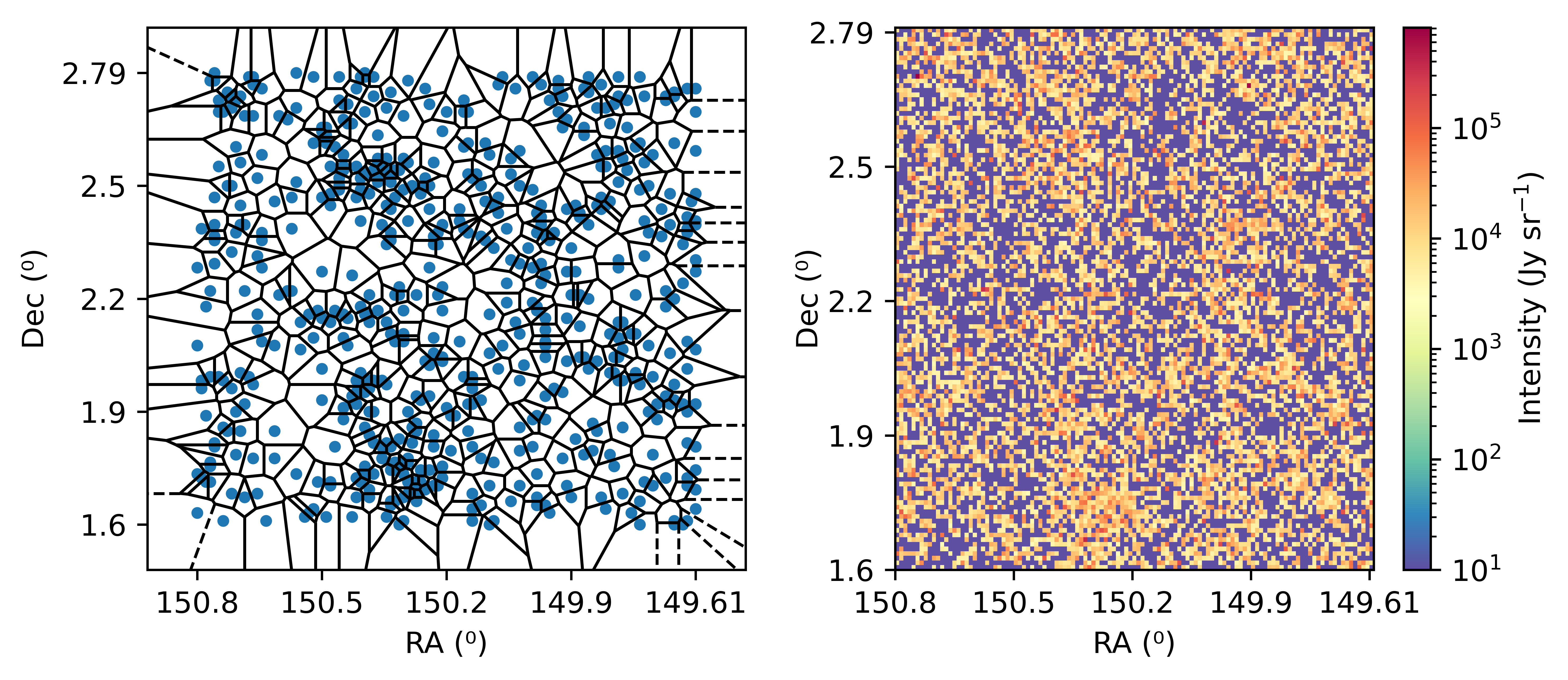
Figure 14: Example VT map when applied to the m4 FARMER LP map at $3.42<z<3.87$. We typically use 3D weighting maps, however we show this example in 2D for clarity. Here this example takes nodes (blue) as the top 3% brightest pixels.

Once we have finished extrapolation, we take these enhanced samples and run the same procedures as in Sects. 2.5 and 2.6. When using the samples extrapolated using a [CII] luminosity function, we only apply the [CII] model which was used to create the corresponding luminosity function.

However, there are significant limitations with this technique. In many cases we can produce multiple valid Schechter fits for a given function as demonstrated by Figure 13, thereby adding different numbers of extrapolated galaxies and altering the resulting power spectra. In the ‘overestimate fit’, a vastly unrealistic number of galaxies were extrapolated due to the steep gradient of the fit, in this case half a million galaxies in a $1.2\times 1.2\deg^{2}$ area per 0.1 dex band. While we found negligible differences between the power spectra for the other fits, the shot-noise for the overestimate fit was inflated by at least 0.2 dex. Furthermore, the minimum mass or luminosity point for extrapolation was unknown, as we do not know the properties of the faintest galaxies at high redshift. Nevertheless, we calibrated these end points by investigating the smallest dwarf galaxies in the local universe, where we found [CII] luminosities as low as $10^{4}L_{\odot}$ and stellar masses as low as $10^{6}M_{\odot}$ (e.g. Cormier et al. 2015; Madden et al. 2013). As it is unlikely that the Schechter function accurately predicts galaxy numbers for the very dimmest galaxies, we only extrapolated down to $10^{5}L_{\odot}$ or $10^{7}M_{\odot}$. In addition we experimented with the end points $10^{7}L_{\odot}$ or $10^{8}M_{\odot}$, which are the end point of [CII]-metallicity relations (De Looze et al. 2014; Lagache 2018) and a typical dwarf galaxy mass respectively. We found minimal differences between the power spectra from these different extrapolation depths for most fits in Fig. 13, so it is likely that the contribution of signal from the smallest galaxies is negligible. The primary exception to this trend is the overestimate fit, where the clustering signal is greatly inflated at $k<10^{0}\,\textrm{Mpc}^{-1}$ when we extrapolate to $10^{5}\,L_{\odot}$. As discussed in Sect. 3.2, this is due to faint galaxies greatly contributing to the clustering signal. Therefore we only included fits that do not demonstrate this dramatic increase in shot-noise and clustering signal. However there were still multiple valid fits in some cases, and while this is not a problem for the final power spectrum magnitude, we discuss constraining these fits further with additional data in Sect. 5.

4.3 Voronoi tessellation for galaxy distribution

Once we generated the additional galaxies via extrapolation, we determined the new galaxies’ map positions and redshifts. Instead of determining these co-ordinates randomly, which was appropriate for adding galaxies in the small stellar mask areas but would destroy any of the existing structure within the intensity cube, we implemented a weighting cube. This is an array that has the same dimensions of the intensity cube and stores relative weights in each voxel, which then calibrate the random selection of $x$, $y$ and $z$ co-ordinates for the extrapolated galaxies. The weights are the normalised stellar mass of FARMER LP’s galaxies, and are stored within the voxels in the same way that [CII] intensity is stored within the intensity cube. We also added a proportion of a galaxy’s weight to voxels on the same redshift slice within two spaces, to prevent over-weighting to specific pixels. The ratio of weights of ‘central pixel’:‘adjacent pixel’:‘pixel two spaces away’ is 3:2:1. Furthermore, we added a baseline weight equivalent to adding an average galaxy to each voxel. This method was inspired by and produces similar maps to Voronoi tessellation (VT) (e.g. Ramella et al. 2001; Kim et al. 2002), which determines overdensities and voids by identifying bright nodes on a map and drawing equidistant lines between them. An example of this applied to FARMER LP is shown in Fig. 14, where we treat high weight voxels as nodes. In this way the highest mass galaxies of FARMER LP (primarily SFGs) become the bright centers of large galaxy clusters within the assumed dark matter halos. This process assumes the majority of extrapolated dim galaxies lie within these clusters, however does not meaningfully account for other structures such as cosmological filaments. Consequently we must therefore exercise caution when viewing the strength of clustering signal in spectra from extrapolation, which we discuss in Sect. 5. We also discuss the impact of VT on power spectra compared to randomly distributing galaxies in Appendix B, to ensure that our initial assumptions are somewhat reasonable.

It would be ideal to use a weighting cube based on known overdensities in the COSMOS field, however at time of publication we only have a proto-cluster density map for $6<z<7.7$ (Brinch et al. 2023). As this would only apply to the redshift band $6.75<z<8.27$, which is unlikely to give useful results as previously discussed, we did not explore this further.

4.4 Power spectra and error analysis for extrapolated sample

After extrapolating from FARMER LP, we can create power spectra from these expansions to the existing samples. When comparing the spectra from different extrapolation techniques in Fig. 15, we find a consistent increase in magnitude for all methods. This is to be expected as extrapolating the missing low mass or low luminosity galaxies produces fundamentally similar outcomes, as low mass galaxies are likely to be dim. The power spectra magnitude increase is relatively small at low redshift ($0.2-0.4$ dex at $3.42<z<3.87$) but is more significant at high redshift ($0.5-0.8$ dex at $5.34<z<6.31$). This is consistent with the idea that FARMER LP is more complete at lower redshift bands, as the survey was able to find a higher proportion of dim galaxies, so extrapolation has more impact for higher redshift sub-samples with worse completeness. When examining the clustering component we find a small increase due to the large number of dim galaxies added around assumed clusters using VT. For example, in $3.42<z<3.87$ we find that transition region occurs around $k\approx 0.25$ for all extrapolation methods, that is, where the clustering signal is approximately equal to the shot-noise component. However, these transition regions are still at smaller $k$ when compared to the simulation work of Karoumpis et al. (2022), a result that is somewhat surprising considering our attempts to mimic larger structure. This may be a consequence of the specific assumptions we made when applying VT because of the lack of frame of reference we have for high redshift structures, as discussed in Sect. 5. In addition, this could result from previous literature deliberately seeding their galaxies around specific dark matter halos.

To verify that this extrapolation method leads to results consistent with the literature, we must directly compare their power spectra. In our figures such as Fig. 16 we only used the mass function extrapolation sample from Weaver et al. (2023) for clarity, however the conclusions are the same for all extrapolation techniques. Overall we find significant overlap between our models and the previous literature at all redshifts. This is demonstrated by our models managing to reach the shot-noise component of all models from previous literature. We also visualise this by showing the non-absolute upper and lower limits from extrapolation when using wide bins, with results shown in Table 4. Furthermore, almost all of our models exceed the expected FYST sensitivity limit, an alternate measure predicting detectability, which implies that (were our extrapolated samples to be accurate to reality) we would be able to recover usable results. This concordance is therefore useful in demonstrating that extrapolating from existing samples (which are useful for absolute lower limits) can be used to replicate predictions where dim galaxies have a significant impact (therefore providing reasonable upper limits). Consequently, existing catalogs can model power spectra from LIM in a variety of test scenarios.

However, there are some caveats to the results from extrapolation. $6.75<z<8.27$ remains an outlier, with spectra at that redshift being multiple dex above some predictions at the same redshift. This is because COSMOS 2020 only includes high luminosity galaxies in this redshift range, so the fits and subsequent extrapolation from the existing sample produced a vast number of galaxies and thereby skewed the power spectra magnitude. We see this in the Schechter fit parameters in Table 8, where the ‘knee’ of the Schechter fit, $L_{\textrm{c}}$, is far higher for most models at this redshift. At lower redshifts, only the ALPINE models (m1-m4) reach the magnitudes of the higher magnitude models from the previous literature, with all our other models only overlapping with the lower estimates. This may be a consequence of these models being fitted using high-luminosity data, and thus produce high luminosities even when applied to smaller galaxies. Therefore it may be best to view these uppermost limits of our work with a level of caution. Despite these discrepancies, and the differences in clustering signal, it is reassuring to see this overall agreement between the sample extrapolated from FARMER LP and the previous literature. In this way, our extrapolation methods are a viable way to create extensions from existing samples.

	$k^{3}P(k)/2\pi^{2}$ ((Jy sr-1)2)
$k$ (Mpc-1)	0.25-0.55	0.55-0.85	0.85-1.15	1.15-1.45
	Lower limits from extrapolation
$3.42<z<3.87$	4.79$\times 10^{6}$	2.49$\times 10^{7}$	6.93$\times 10^{7}$	1.52$\times 10^{8}$
$4.14<z<4.76$	3.48$\times 10^{6}$	1.81$\times 10^{7}$	4.91$\times 10^{7}$	1.11$\times 10^{8}$
$5.34<z<6.31$	6.98$\times 10^{5}$	3.29$\times 10^{6}$	9.19$\times 10^{6}$	1.91$\times 10^{7}$
$6.75<z<8.27$	8.68$\times 10^{5}$	3.87$\times 10^{6}$	1.11$\times 10^{7}$	2.50$\times 10^{7}$
	Upper limits from extrapolation
$3.42<z<3.87$	3.98$\times 10^{8}$	2.13$\times 10^{9}$	6.02$\times 10^{9}$	1.31$\times 10^{10}$
$4.14<z<4.76$	1.75$\times 10^{8}$	8.92$\times 10^{8}$	2.51$\times 10^{9}$	5.38$\times 10^{9}$
$5.34<z<6.31$	2.30$\times 10^{8}$	1.10$\times 10^{9}$	3.08$\times 10^{9}$	6.47$\times 10^{9}$
$6.75<z<8.27$	81.59$\times 10^{7}$	7.15$\times 10^{7}$	2.04$\times 10^{8}$	4.58$\times 10^{8}$

Table 4: Soft lower and upper limits of FARMER LP power spectra found from the Weaver et al. (2023) mass function extrapolated sample, using $\Delta k=0.3$ Mpc^-1, as shown in Fig. 16. The upper section describes lower limits, the lower section describes upper limits. The lower limits are Si15 for $3.42<z<3.87$ and $4.14<z<4.76$ and Sc20 for other bands, whilst the upper limits are m3 for all bands.

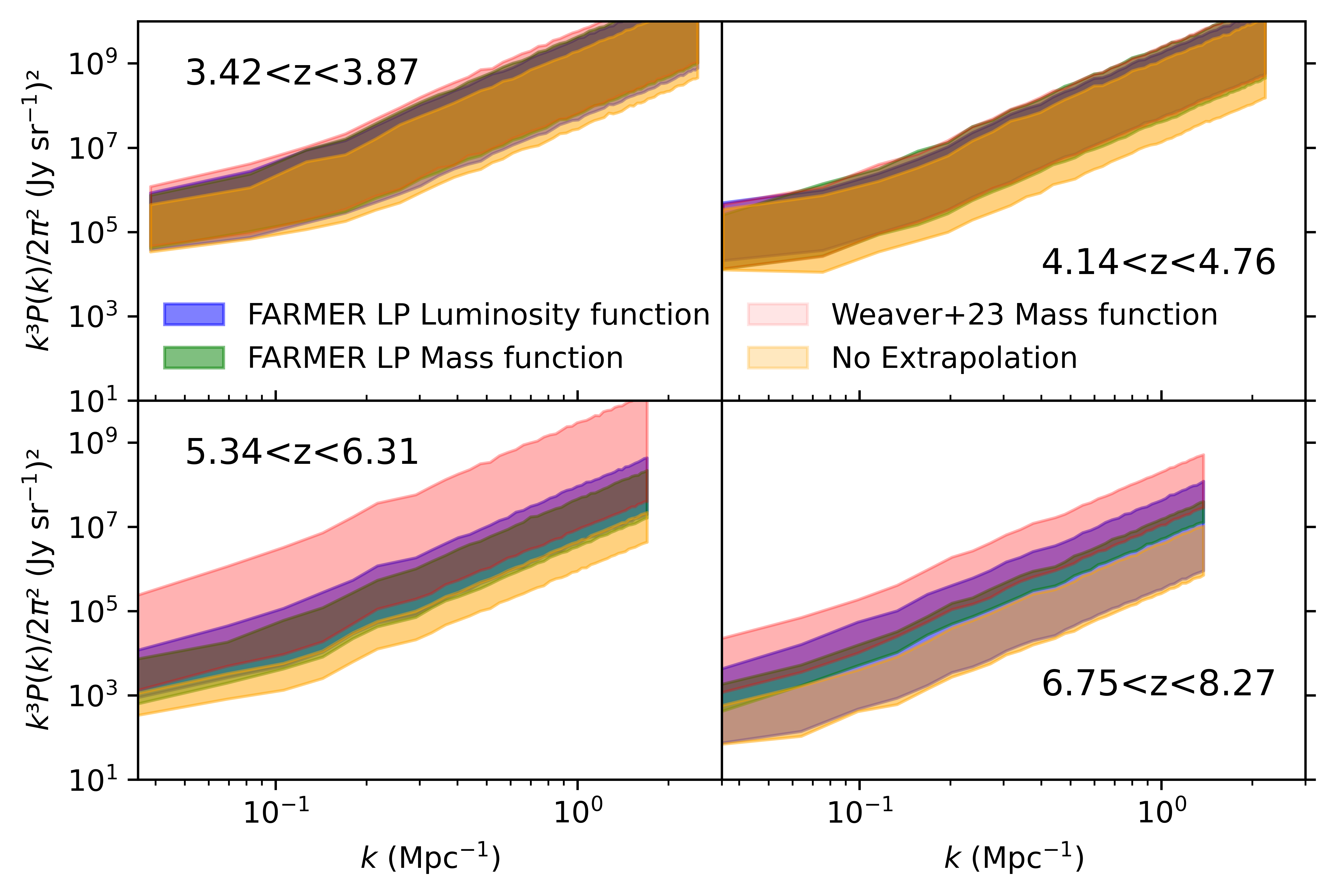
Figure 15: Comparison of extrapolated power spectra from different extrapolation techniques. The models in orange are those from the original FARMER LP sample with no extrapolation, with blue representing FARMER LP luminosity function extrapolation, green representing FARMER LP mass function extrapolation, and red representing mass extrapolation using Weaver et al. (2023) parameters. The key point here is the difference between extrapolated models and the original sample in orange.

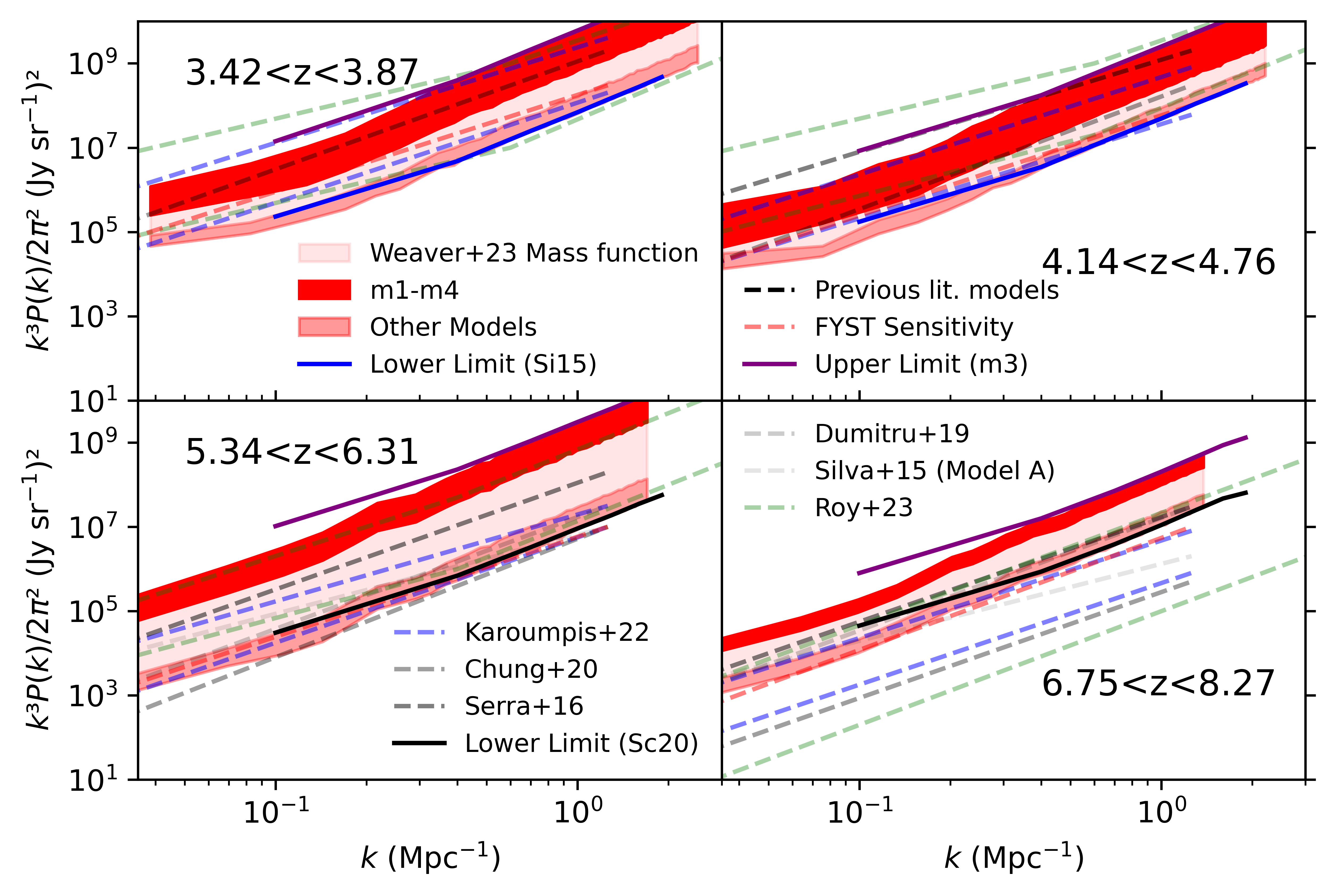
Figure 16: As Fig. 10, but for the extrapolated data based on the mass function fit with parameters given by Weaver et al. (2023). We group the ALPINE models together and increase shade density for emphasis.

We also applied the same error analysis methods for the extrapolated samples, focusing on the mass function extrapolation using Weaver et al. (2023) to maintain consistency, resulting in Fig. 17. This figure shows that all models have greater S/N in comparison to the original versions in Fig. 11. This is especially clear when using wider bins as all models give S/N$>$1 for all redshift bands. Therefore, in the scenario where these samples accurately reflect reality, observations should be possible when using wider bins for all redshift ranges as has been predicted by prior work. When using narrow $k$ bins, the ALPINE models consistently have S/N$>$1, however the other models do not breach this barrier even at the lowest redshift. We can alternatively view this as models working for no redshift bands (previous literature models) or all redshift bands (ALPINE models). This clear divide is somewhat surprising, as we would expect to recover usable results for all models at the lower redshifts, and other works such as CCAT Collaboration (2023) expected no models to work for $6.75<z<8.27$. Regardless, in order to guarantee detections instruments must use wider $k$ bins, which reduces the ‘resolution’ of our results. However, even with this drawback it is still likely that we will be able to recover usable results within our initial observation period, assuming these more complete extrapolated samples reflect reality.

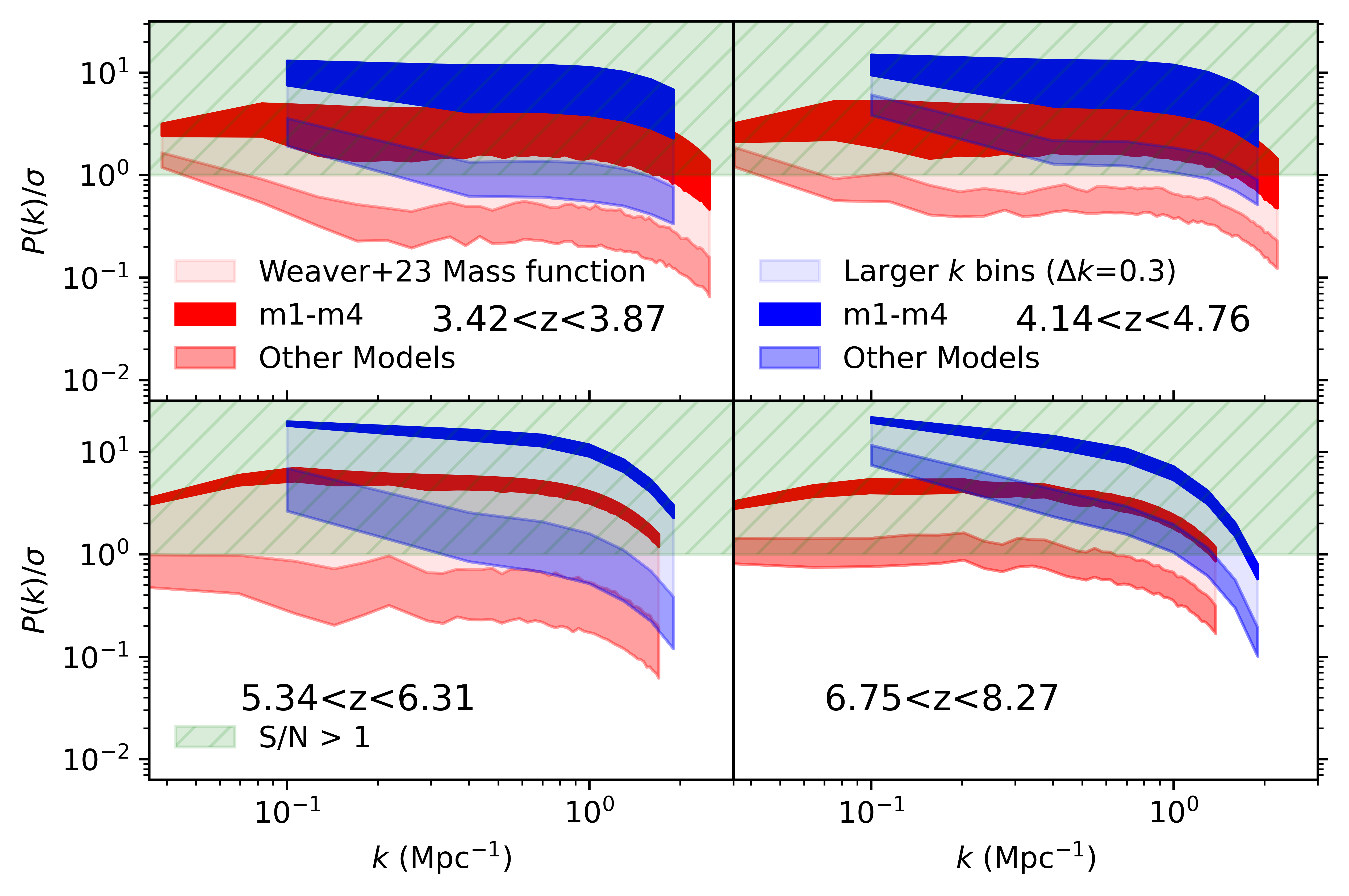
Figure 17: As Fig. 11, but for the extrapolated data based on the mass function fit with parameters given by Weaver et al. (2023). The specific shaded region is for the ALPINE models m1-m4.

5 Discussion

In this study, we have demonstrated the feasibility of generating meaningful constraints on line intensity mapping (LIM) power spectra for a specific field, employing empirical data from a known sample and [CII] luminosity models based on galaxy bulk property data. In addition, it is also possible to extend this sample via plausible extrapolation methods to create reasonable limits for these spectra, which are consistent with the power spectra of previous simulated work. This approach shows promise for making predictions in other fields, provided that we can use samples with bulk properties across sufficiently extensive and deep volumes. Moreover, we have identified several opportunities to refine our methodology, using forthcoming data and preliminary findings from the EoR-Spec DSS. These potential improvements are explored in detail below.

When solely using empirical data, the lower limits on power spectra we established in Table 2 are primarily beneficial for forecasting observations with EoR-Spec. However, these can also be related to previously conducted simulations (e.g., Fig. 10), and our analysis confirms that all previously reported power spectra exceed our absolute lower limits. Notably, some of these spectra fall beneath our m3 and m4 models within the redshift intervals $3.42-3.87$ and $4.14-4.76$, which we attribute to inherent biases in these models discussed later.

However, the expected observations’ S/N under EoR-Spec’s parameters registers below 1 across most $k$ (Fig. 11), even with wide binning for the majority of models. Furthermore, extensive masking beyond $z>6.3$ obliterated any features of large-scale structures which existed within the COSMOS field, leaving only the most luminous star-forming galaxies (SFGs) in COSMOS 2020. As a result, for the redshift range $6.75-8.27$, we can only draw conclusions from the small-scale regions. Even still, the observed magnitudes may be influenced by a preferential bias towards brighter galaxies. Consequently, we find that employing this methodology in fields with significant voids is impractical.

The absolute minimum constraints we derived serve as conservative limits for potential outcomes of future observed LIM cube spectra, and therefore are valuable for observational planning. However, to address the limitations presented by these conservative estimates, we adopted an extrapolation approach to mitigate the incompleteness in our datasets and to produce more comprehensive samples. While our specific procedure relates to the existing COSMOS 2020 catalog, for example CANDELS lies within the COSMOS field, this methodology should be adaptable to other datasets and observational fields. Encouragingly, the results shown in Fig. 16 demonstrate that our models’ shot-noise components align with the previous work, suggesting the number of galaxies extrapolated from the FARMER LP is appropriate. Despite this, only the ALPINE models m1-m4 reach the uppermost predicted limits, which suggests that these models and similar prior analyses may be overly optimistic.

Due to the extrapolation adopted here and the corresponding substantial assumptions used to extend beyond purely empirical data, the upper limits presented in Table 4 are less stringent than our absolute lower bounds. Consequently, the shot-noise component in extrapolated spectra is a valuable but not infallible indicator for forecasting observational results and comparing to previous work. The clustering signal is weaker relative to prior simulations, likely due to discrepancies between our clustering assumptions for VT in Sect. 4.3 and those employed in prior work. However, because of the uncertainty surrounding the accuracy of these prior works’ clustering assumptions, this is a challenging obstacle based on incomplete information. Future work will focus on refining this aspect, considering alternative weighting methodologies for VT and closely comparing our clustering assumptions with those from previous studies. Additionally, the incorporation of overdensity maps similar to those proposed by Brinch et al. (2023) could enhance the accuracy of our predictions, using data from forthcoming analyses or initial EoR-Spec observational results to offer a more robust framework for understanding galaxy clustering within LIM.

Analyzing the S/N of our extrapolated models reveals that utilizing wider $k$ bins consistently achieves S/N$>$1 across all models and redshift intervals, suggesting that detecting a signal in actual observational scenarios is highly probable. However, for narrower $k$ bins, only the ALPINE-based models (m1-m4) maintain an acceptable S/N across various redshifts. In contrast, other models exhibit poor S/N at all redshifts, even with our assumption of 100% observational efficiency. Aside from implying that the lower limits of power spectra may be challenging to distinguish using EoR-Spec, the acceptable models are all based on ALPINE data which significantly deviate from the standard [CII]-SFR models. The power spectra of these models show a more pronounced decrease in magnitude with redshift compared to others, potentially due to them being derived from galaxies with high [CII] luminosity. This carries an underlying assumption that all galaxies exhibit substantial [CII] emission, leading to a rapid decline in signal as the galaxy count decreases. These ALPINE galaxies are also not representative of the redshift ranges $3.42<z<3.87$ and $6.75<z<8.27$, rendering the highest limit estimations for these intervals (based on model m3) questionable. While we believe that incorporating a variety of [CII] emission models is crucial, with models m1, m3, and m4 exploring the conceptual space where [CII] emission is stronger in high-redshift galaxies when compared to the current universe, their discrepancy with the existing literature is clear. Model m2 is the exception to the other ALPINE models, as it posits a linear log-log relationship between [CII] and stellar mass thereby aligning more closely with the literature’s [CII]-SFR models. In future work we plan to continue utilizing these models while also investigating strategies to address the limitations presented by ALPINE data, such as its restricted redshift coverage, bias towards star-forming galaxies (SFGs), and UV-selection criteria. Additionally, we aim to incorporate [CII] data from higher redshifts, such as from REBELS (Bouwens et al. 2022) upon its full public release, to enhance our models’ comprehensiveness and accuracy.

An inherent challenge with the extrapolation process lies in the uncertainty in determining the fit parameters for Schechter functions. While it is feasible to fit a Schechter function to the high-luminosity upper knee section after applying CANDELS extrapolation, the scarcity of data at lower masses and luminosities introduces ambiguity in identifying appropriate fits. Our approach was to select fits that minimized errors according to least-squares fitting procedures and with gradients that were in alignment with previous studies, such as those reported by Weaver et al. (2023). This was to prevent extrapolating a physically impossible number of galaxies, such as cases which would add millions of galaxies per 0.1 dex interval. In most scenarios the differences in the resulting power spectra are minimal, as illustrated in Fig. 13, however it would be ideal to constrain these fits using datasets that offer more comprehensive coverage of the mass and luminosity functions. Upcoming surveys such as COSMOS-Web (Casey et al. 2023; Franco et al. 2023; Silverman et al. 2023) and other deep pencil field studies are expected to provide insights into the fainter ends of these functions, thereby serving as valuable benchmarks for calibrating Schechter curve fits. In this way we expect to enhance the reliability and accuracy of extrapolations used in future analyses.

Our foundational methodology is sound, however we must integrate additional variables to increase precision in forecasting upcoming observations, which we omitted in this work to maintain consistency with the previous literature. Line intensity mapping (LIM) inherently measures aggregate signals and thus includes interlopers within the cubes, such as CO and [OIII] line emission from galaxies at different redshifts. These should subsequently be isolated and removed using foreground signal elimination techniques, such as cross-referencing with catalogs of galaxies identified at higher resolution. It is one of EoR-Spec DSS’s objectives to cross-correlate LIM data from various lines, as highlighted by Visbal & Loeb (2010) and Chung (2022). We must also account for various complex noise sources, including atmospheric noise, the influence of the instrument’s scanning pattern, and the masking of specific areas. Ongoing research endeavors, such as those by Karoumpis et al. (in prep.) addressing CO foregrounds, Dev et al. (in prep.) applying frameworks like Time Ordered Astrophysics Scalable Tools (TOAST) for atmospheric noise and scanning strategies, and Roy & Battaglia (2023) examining cross-correlation’s impact on S/N, are actively addressing these challenges. Each issue presents its unique set of complications, which makes gauging errors increasingly complex — for example, CO interlopers pose significant challenges at lower frequency, whereas atmospheric noise predominantly affects higher frequency channels. Fortunately, the early FYST science data will serve as a valuable resource for calibrating our error estimations. Employing techniques such as cross-correlation and atmospheric de-striping will likely alleviate major error sources. Furthermore, as there will be varying levels of sensitivity over the 2000 hours observation period of EoR-Spec (CCAT Collaboration 2023), our methodology enables the generation of distinct predictions for various observation phases, enhancing the applicability of our forecasts.

Our investigation is tailored to the regions observed by EoR-Spec DSS, thereby restricting its scope as we require samples covering a sufficiently large sky area ($\sim$1 $\deg^{2}$) with comprehensive bulk property data within the E-COSMOS or E-CDFS regions. Currently, our analysis is confined to using COSMOS 2020, as the CANDELS/GOODS-S dataset (Hsu et al. 2014) lacks the necessary scale to accurately assess large-scale clustering signal. However, upcoming data from the Euclid mission (Euclid Collaboration 2022) will extend over 20 $\deg^{2}$ in the GOODS-S field at appropriate redshifts, thereby allowing for the generation of meaningful predictions for this field. In the interim, we can also use our method to project shot-noise estimates for experiments covering smaller areas, such as TIME and CONCERTO. Additionally, we can also examine the relative impact of individual large galaxy clusters on the power spectra, using both observed and simulated clusters for this analysis. LIM’s capability to survey wider fields makes these clusters, for instance the CRLE and AZTEC-3 protoclusters (Riechers et al. 2010; Capak et al. 2011; Pavesi et al. 2016; Vieira et al. 2022), a key focus for subsequent simulations and future research. This could be achieved by incorporating simulated clusters into our maps to determine their relative impact on the power spectra. Finally, we also plan to delve into additional analytical techniques that can be applied to Fourier-transformed cubes, such as delta-variance and bi-spectra statistics. These approaches hold the potential to reveal further insights, enriching our understanding of the underlying cosmic structures.

6 Conclusion

In this work, we introduced an empirically-based methodology for creating mock [CII] line intensity mapping (LIM) cubes using an existing sample, in this case the FARMER LP sub-sample of the COSMOS 2020 galaxy catalog. This approach enabled us to make power spectra predictions for the E-COSMOS field, which will be surveyed by the EoR-Spec Deep Spectroscopic Survey (DSS) during its 2000-hour campaign commencing in 2026. These LIM cubes were tailored to the observational specifications of the EoR-Spec instrument aboard the Fred Young Submillimeter Telescope (FYST). Given the sample’s incompleteness toward faint galaxies, the resulting power spectra establish lower bounds, which are quantified for $k=1\,\textrm{Mpc}^{-1}$ as $P(k)/2\pi^{2}=3.06\times 10^{7},\,1.43\times 10^{7},\,9.80\times 10^{5},\,2.77\times 10^{5}\,$(Jy sr${}^{-1})^{2}$ across the redshift intervals $3.42<z<3,87$, $4.14<z<4,76$, $5.34<z<6,31$, $6.75<z<8,27$, respectively (Table 2). Furthermore, we develop techniques to extrapolate from this dataset, producing results similar to previous simulations.

These simulated LIM cubes incorporate [CII] luminosity models from the previous literature as well as those derived from ALPINE data, including models that deviate from linear log-log [CII]-SFR relationships. The models were applied across four aforementioned redshift bands to create a map spanning $1.2\times 1.2\deg^{2}$. The key findings from our work are summarised as follows:

• We created four [CII] models solely using ALPINE galaxy bulk property data, which diverged from the conventional linear log-log [CII]-SFR relationship. These models produce power spectra with a range of $\sim$1 dex, and are consistent with existing [CII] models when applied to the FARMER LP sub-sample. However, these models are less constrained at redshift ranges beyond ALPINE’s redshift coverage ($3.42<z<3.87$ and $6.75<z<8.27$).

• Our approach can generate mock LIM cubes using available galaxy catalogs, such as COSMOS 2020. Given the incompleteness of these samples at the faint end of the luminosity function, the resultant power spectra serve as lower bounds, reflecting only the galaxies that have been detected. All previous power spectra from the literature exceed these minimum values for z$<$6.3. Our results are less conclusive above this point, due to the greater level of incompleteness of COSMOS 2020 at higher redshifts.

• We evaluated the impact of incompleteness from the variance in power spectra between the original sample and prior predictions, and extrapolated from the empirical dataset in FARMER LP by considering truncated mass and luminosity functions along with the detection rate ratio between the CANDELS data and COSMOS 2020. This extension from the original sample increases the magnitude of our empirically-guided mock power spectra by approximately 0.5 dex, placing them within the range of earlier simulations. Aside from providing this concordance, the extrapolation also offers a tool to estimate the signal strength for forthcoming observations. From this we can identify potential power spectra ranges allowed by previous predictions which are only reached by specific ALPINE models, that therefore are less likely to reflect the signal strength to be observed.

• In our power spectra from extrapolations, we predict signal-to-noise ratios S/N$>$1 only when using wide spatial frequency bins ($\Delta k=0.3$ Mpc^-1). However this assumes 100% signal recovery efficiency, so future investigations will necessitate a more detailed consideration of foreground line signals and atmospheric noise.

This work provides empirical support for the previous simulation work. While the anticipated challenges in observations will be significant at higher redshift bands, we remain confident that the planned FYST/EoR-Spec surveys will be able to obtain significant constraints for $z<6$. Future efforts will extend this work to include realistic foregrounds, and to obtain more solid constraints at z$>$6 based on incoming JWST and Euclid data in the COSMOS field.

Appendix A ALPINE model checks

When creating the ALPINE [CII] models, we attempted to fit Eq. 2 to all combinations of bulk properties. We performed this fitting for the individual galaxies in the sample as well as binned galaxies using least-squares fitting procedures. When binning we used 5 bins with 13 galaxies each, bins being sorted by [CII] luminosity, stellar mass, SFR, or metallicity. This produced a vast number of models, most of which were poor fits, so we applied multiple checks:

• We calculated the reduced chi-squared statistic ($\chi^{2}_{\nu}$) for each model as described in Eq. 20, where $\nu$ is the number of degrees of freedom, $L_{[\textrm{CII}],i}(X)$ is the [CII] luminosity of each data point with bulk properties $X$, $L_{\textrm{[CII], model}}(X)$ is the [CII] luminosity given by the model when substituting in the same bulk properties $X$, and $\sigma_{i}^{2}$ is the error in [CII] luminosity for each data point. When calculating this for a binned fit, we performed error propagation to find $\sigma_{i}^{2}$, and we took $X$ as the averaged bulk properties of each galaxy within the bin. We took the number of degrees of freedom $\nu$ as the number of fit parameters subtracted from the number of data points. A model was viewed as acceptable when its $\chi^{2}_{\nu}$ is within $4\,\sigma$ of the expected value for a good model, 1. This is when we are within the limits set by Eq. 21, where we set the number of $\sigma$ $n=4$ and $\nu$ depends on the model. This has a large amount of leniency, however we use this limit to allow as many models as possible. For example, m1 has 4 fit parameters, and was calculated from binned data (5 data points), so $\nu=5-4=1$. As $n=4$, the limit $\chi^{2}_{\nu,\textrm{ n}\sigma\textrm{ limit}}=6.65$. This statistical concept is described in detail in the literature (for instance Hughes & Hase 2010, pg. 102-107).

$$\chi_{\nu}^{2}=\frac{1}{\nu}\sum_{i}\left[\frac{L_{\textrm{[CII], model}}(X)-L_{[\textrm{CII}],i}(X)}{\sigma_{i}}\right]^{2}$$ (20)

$$\chi_{\nu,\textrm{ n}\sigma\textrm{ limit}}^{2}=1+n\sqrt{\frac{2}{\nu}}$$ (21)

• For each model we checked if it diverged significantly from the expected range of [CII] luminosities when using outlier values, i.e. above $10^{13}L_{\odot}$ or below $10^{4}L_{\odot}$. We inserted the maximum and minimum values of galaxy bulk properties within FARMER LP ($3.42<z<8.27$) as shown in Table 5. If a model failed this test it was rejected.

Value	Max	Min
$\log_{10}\left(\frac{M_{\star}}{M_{\odot}}\right)$	6.600	12.002
$\log_{10}\left(\frac{\textrm{SFR}}{M_{\odot}\textrm{yr}^{-1}}\right)$	-4.705	3.807
$\log_{10}\left(\frac{\textrm{sSFR}}{\textrm{yr}^{-1}}\right)$	-14.756	-7.337
$\frac{Z}{12+\log\textrm{(O/H)}}$	5.822	9.083
$\log_{10}\left(\frac{Z}{12+\log\textrm{(O/H)}}\right)$	0.765	0.958

Table 5: Maximum and minimum bulk properties within the FARMER LP sample, used for model testing.

• It was important to determine if each model was consistent with the known ALPINE [CII] luminosities when applied to the COSMOS 2020 data. We applied the test models to FARMER LP data in the same redshift range as ALPINE ($4.4<z<4.65$ and $5.05<z<5.9$), calculated the histograms of the resulting [CII] luminosities, and fitted a Gaussian distribution to the histograms, which we compared to the equivalent distribution of the ALPINE [CII] data. If these distributions had similar means and standard deviations ($<20$% difference), we accepted the model. This is demonstrated for our successful models in Fig. 18.

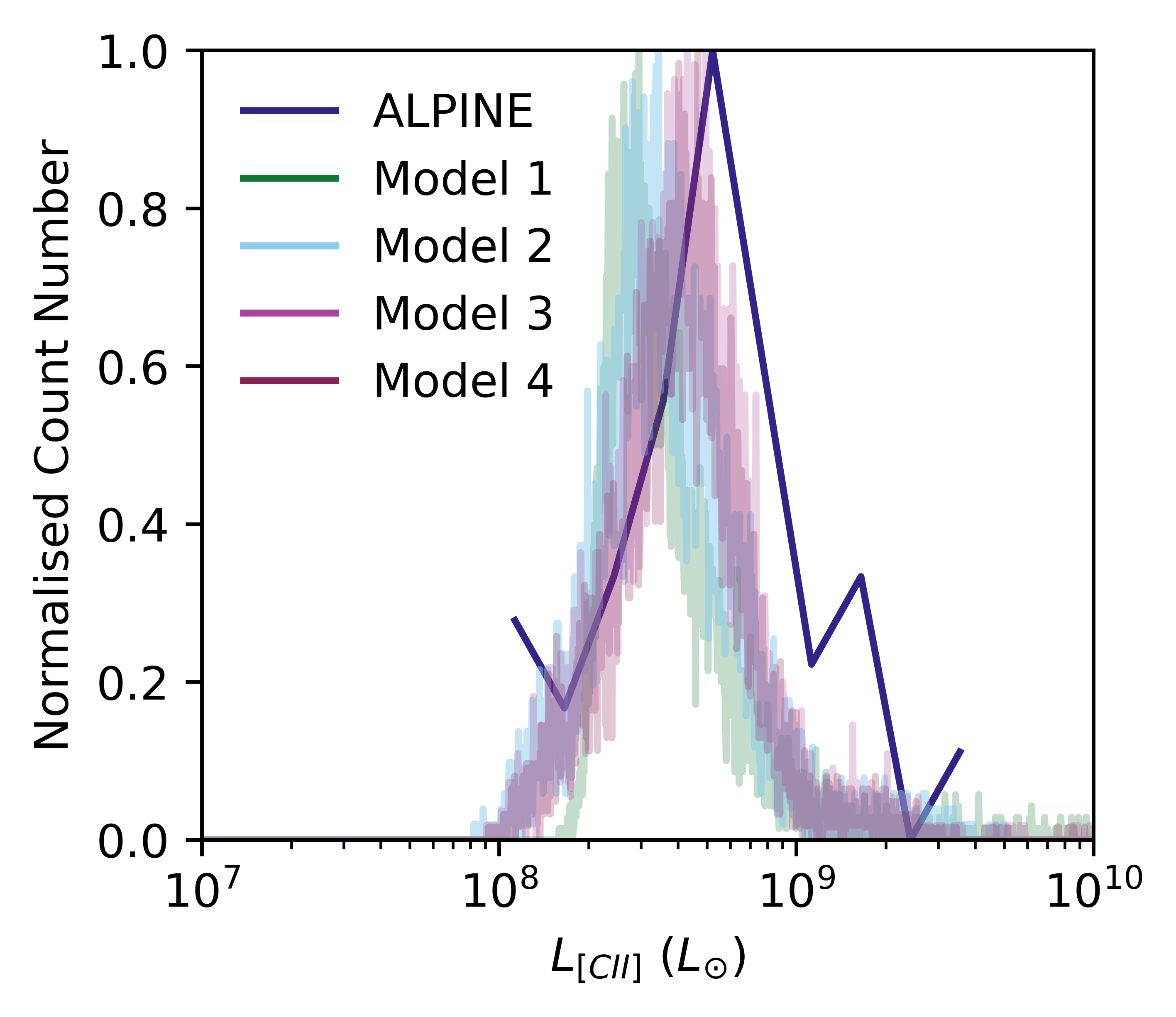
Figure 18: Comparison of the histogram of the ALPINE [CII] luminosities compared to m1-m4 histograms when applied to FARMER LP at $4.4<z<4.65$ and $5.05<z<5.9$. As these resemble Gaussian distributions, we made fits to these histograms and compared the means and standard deviations.

• Finally, we checked that each model made basic physical sense. For example, we had a seemingly acceptable test model that was a quadratic in stellar mass - that is, a model that produced high [CII] emission with very high OR very low stellar mass. As this is clearly non-physical when considering the [CII] emission of dwarf galaxies, we excluded this model.

Appendix B Assumptions made for constructing intensity cubes and power spectra

In our methodology we made many assumptions about how we should construct our intensity cubes, which we discuss and justify in this section.

A key assumption in using redshift data from FARMER LP to select which galaxies lie within each band is that the error in photometric redshift does not meaningfully impact the power spectrum. For a non-negligible proportion of galaxies, their photometric redshift errors are greater than the redshift range covered by individual frequency slices. Therefore the galaxy could actually ‘belong’ to a different slice of the 3D intensity cube, or a galaxy may be erroneously included or excluded from the cube, thereby impacting the power spectrum. To check that the power spectra magnitude is unaffected we compared the power spectra of the default FARMER LP (when using Si15), to versions where each galaxy within the sample had its redshift increased by $\sigma_{z}$, redshift decreased by $\sigma_{z}$, or changed by a random fraction of $\pm\sigma_{z}$. Here $\sigma_{z}$ is the error calculated from the 68% confidence limit in photometric redshift. We also used more extreme samples that tried to include or exclude as many galaxies as possible in a given redshift band (within 1 $\sigma_{z}$). As shown in Fig. 19, there is negligible deviation in shot-noise ($<0.1$ dex) for the reasonable variations, with slightly greater deviation in the clustering signal. There are greater changes when using the extreme examples, with shot-noise deviation up to 0.25 dex and clustering signal deviation up to 0.5 dex. While these changes are more perceptible, the samples must be contorted in ways which are extremely unlikely to occur in reality. Consequently we do not believe that deviations caused by photometric redshift errors could impact our results meaningfully.

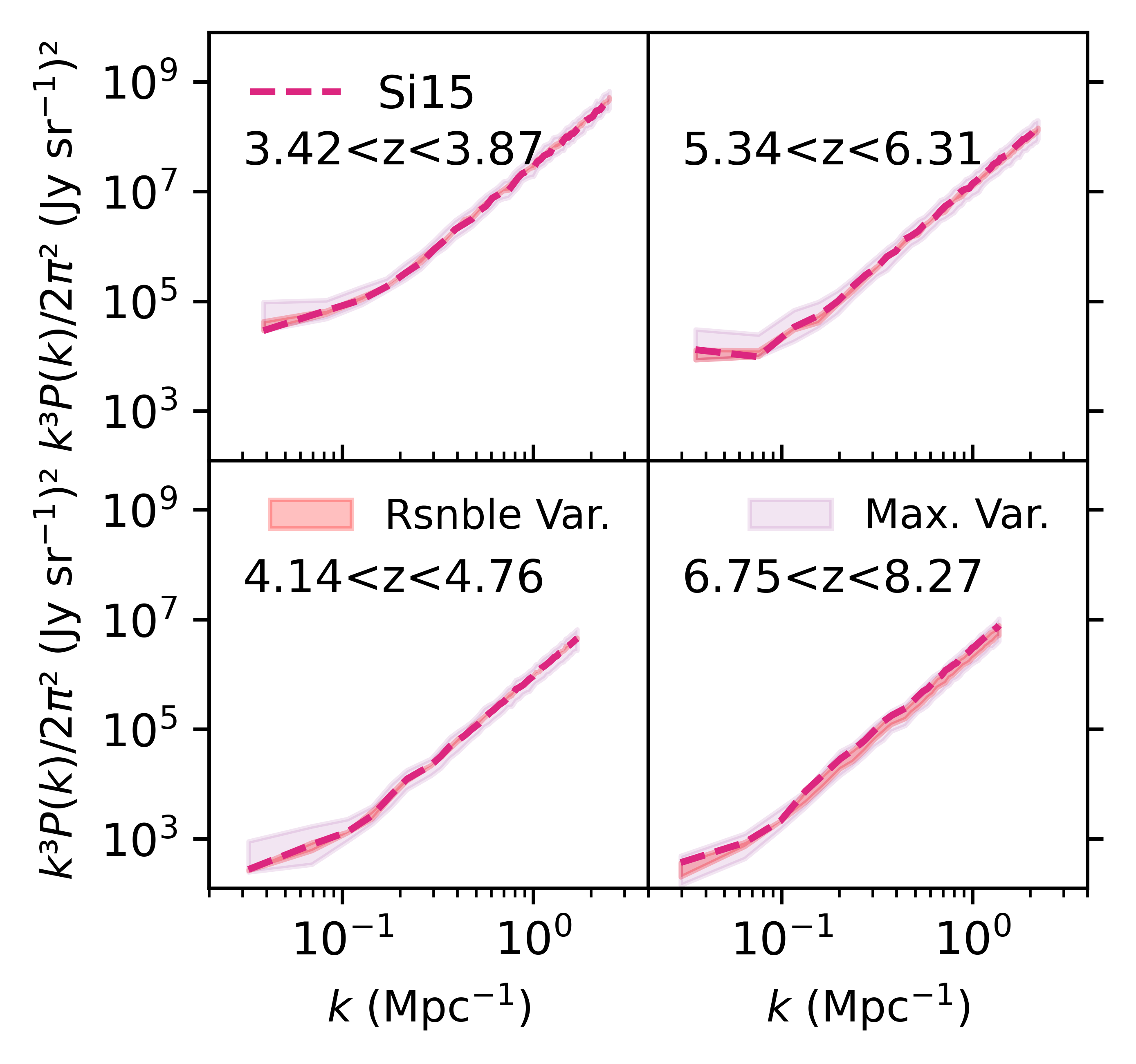
Figure 19: Comparison of the power spectra of Si15 with samples using randomised redshifts. Reasonable variation fits randomise the sample galaxies’ redshifts within one standard deviation, with maximum variation fits including as many or as few galaxies as is plausible. In most cases, the reasonable variation spectra are nearly indistinguishable from the default spectra. We do not include other [CII] models for clarity.

We also assumed that extrapolation within the masked regions of COSMOS 2020 was appropriate, and that by averaging 10 of these power spectra we do not introduce false structure. We verified this by comparing the power spectra of intensity cubes with and without mask extrapolation over all redshift bands using Si15 (Fig. 20). There is negligible difference between the spectra for small $k$ because the areas are too small ($<1$ arcsec²) to meaningfully contribute to large scale structure. When observing shot-noise, there is a small decrease in shot-noise magnitude when we fill the mask ($<0.1$ dex) as the power spectra calculations when masking necessitated shrinking the volume. A decrease in volume of 10%, corresponds to a 0.1 dex shot-noise increase, but as the average intensity per voxel is increased by filling in the mask we instead see a much smaller increase. The only exception for this trend is $6.75<z<8.27$, as the mask covers a much wider area (50%) and therefore we fill in far more signal. Overall, we demonstrated that leaving the stellar mask empty does not change any structural results significantly for $z<6.3$, but marginally overestimates the overall shot-noise of the power spectrum - hence, our assumption is valid. In any case, the calculated power spectra error is much larger than this discrepancy.

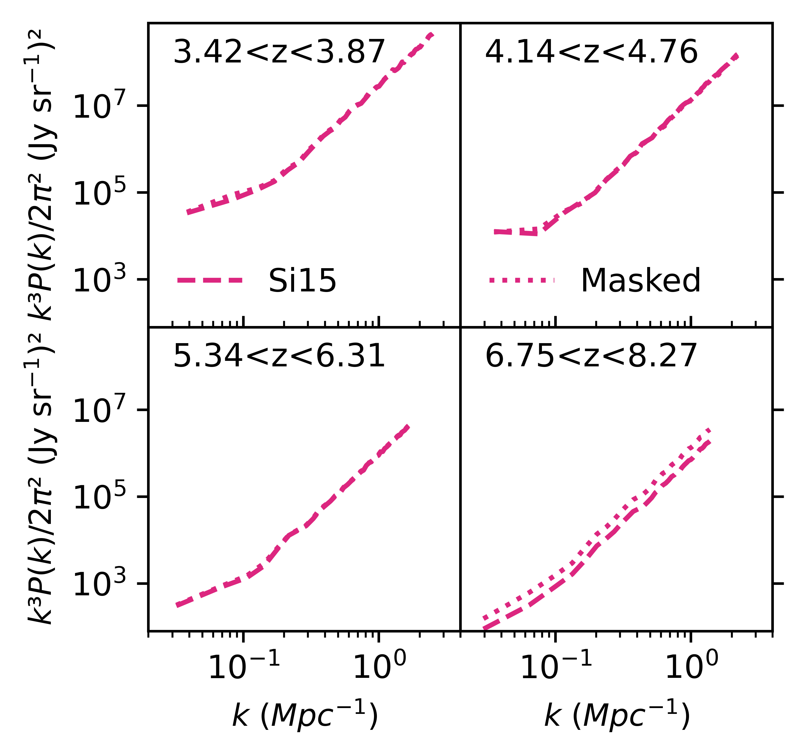
Figure 20: Comparison of the power spectra of Si15 at all redshifts with versions where we did not perform extrapolation to add galaxies in the stellar mask. We do not show other models for clarity. As shown, the change in magnitude is negligible for clustering scales (except for $6.75<z<8.27$).

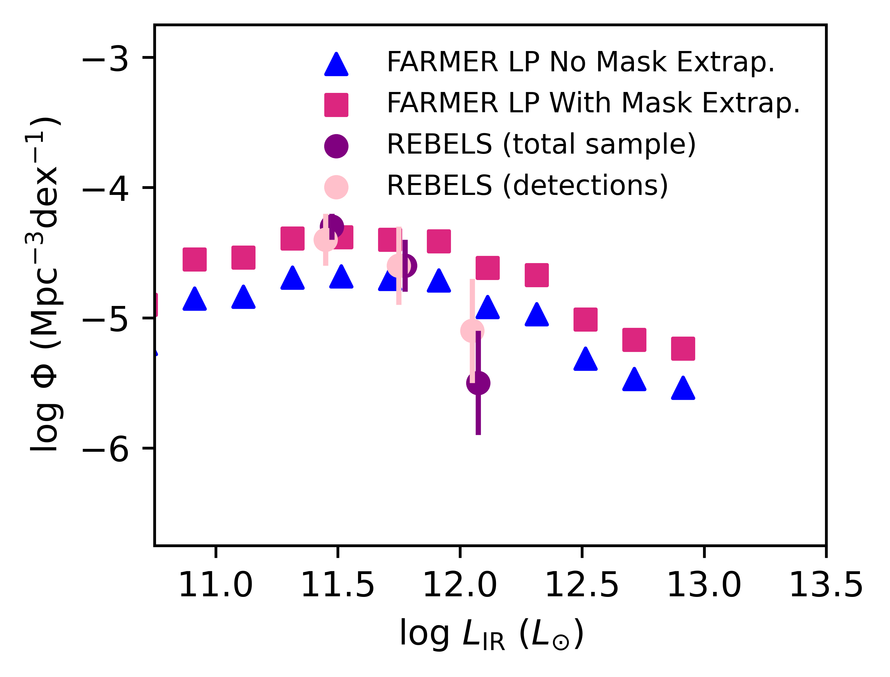
Figure 21: Comparison of the IR luminosity functions of REBELS when using the entire sample or when using only detections, and FARMER LP with and without mask extrapolation. We do not plot the predicted ranges of Schechter functions from Barrufet et al. (2023) due to the limited number of data points. The points of the REBELS functions are at the same luminosity, and are slightly offset in the figure to increase clarity.

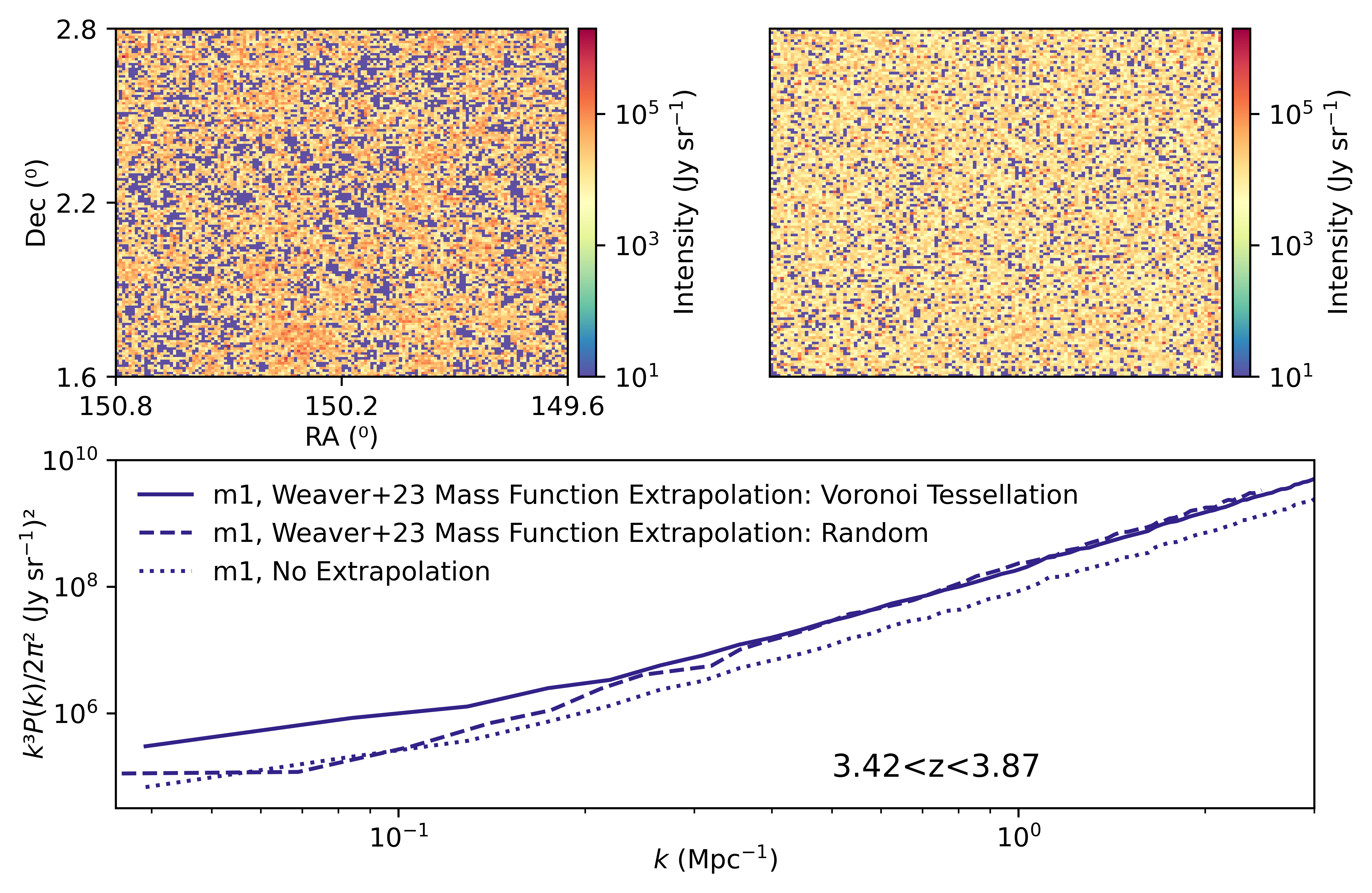
Figure 22: Comparison of power spectra demonstrating the impact of VT on extrapolation. In the left subplot we show a cross-section of the LIM cube at $3.42<z<3.87$ for m1 when using VT to select galaxy location. In the right we see the same, except for the random location selection case. In the lower subplot we compare the power spectra.

The only exception to the previous paragraph is the $6.75<z<8.27$ band, where we take a far greater degree of mask extrapolation and approximately double the original sample. Considering the innate bias towards the brightest galaxies at these distances in FARMER LP, this leads to results that eclipse those from equivalent simulated work (e.g. Fig. 10). This discrepancy is significant and surprising, especially in the context of the other redshift bands where there is greater concordance. In order to investigate whether it is appropriate to apply the standard stellar mask extrapolation principles to the $6.75<z<8.27$ band, we compare the IR luminosity functions of this band and of REBELS (Bouwens et al. 2022), a survey targeting 42 galaxies at $6.4<z<7.7$ including 15 spectroscopically confirmed [CII] sources. We use this sample with its known data as a useful point of reference, even if most of its data do not lie within the COSMOS field, with its IR luminosity function taken from Barrufet et al. (2023). Fig. 21 compares this to the IR luminosity functions of FARMER LP in the $6.75<z<8.27$ band with and without the mask extrapolation, and we find that there is strong agreement in both cases for $L_{\textrm{IR}}<10^{12}\,L\odot$. However, it is clear from a visual examination that the high luminosity end of the FARMER LP luminosity functions would be in disagreement from any Schechter curve that could be fitted to the REBELS data. This is true even without mask interpolation. Correspondingly, we do find it appropriate to be cautious of results at these redshifts. We continued to use the same mask extrapolation methods for this band to ensure consistency with the other redshift bands.

Finally, it is important to retain the existing structure when extrapolating to prevent changes in the clustering signal, so we used the Voronoi tessellation (VT) method as in Sect. 4.3. We validated this technique by comparing cubes and power spectra using m1 at $3.42<z<3.87$, when using no extrapolation, extrapolation with random locations, and extrapolation with locations determined using VT (Fig. 22). For both extrapolations, the shot-noise increase is similar and expected ($\sim$0.5 dex). However the structure component is very different, with the clustering in the random location case regressing to the no extrapolation case, while the VT case shows a relatively large kick. This becomes clear when comparing the intensity cubes, as the random location signal is similar to white noise, while the VT case clearly demonstrates structure. While there is the potential concern of VT over-weighting around the existing galaxies of the sample, this is in fact ideal for us as FARMER LP is likely to include the bright centres of galaxy clusters. Despite this, we find that the clustering signal from our extrapolated samples is weaker in comparison to work from previous literature (Fig. 16, indicating that this method will require refinement and calibration in the future.

Appendix C Power spectra error

As a first estimate for calculating the error in the power spectrum, we included the thermal instrumental noise as well-understood errors in beam smoothing and sample variance, which we briefly discussed in our methodology. This is detailed further by Li et al. (2016) and Chung et al. (2020) where the authors calculate it analytically using Eq. 22:

$$\sigma(k)=\frac{P(k)+P_{\textrm{n}}(k)}{\sqrt{N_{\textrm{modes}}(k,\Delta k)}}\frac{1}{W(k)}$$ (22)

where $P(k)$ is the [CII] power spectra, $P_{\textrm{n}}(k)$ is the power spectra due to thermal noise, $N_{\textrm{modes}}(k,\Delta k)$ is the number of modes that are averaged over to calculate $P(k)$ (i.e. the number of points in 3D $k$ space with $k-\Delta k/2<k<k+\Delta k/2$ where $\Delta k$ is the shell width), and $W(k)$ is a power spectrum attenuation factor for large $k$ caused by the smoothing of the map via the instrumentation beam. The $\Delta k$ we use depends on our use case: for maximum precision we divide the total $k$ range by a number of intervals equal to half the number of pixels across the length of the map, resulting in $\Delta k=0.044,0.040,0.037,0.035$ Mpc^-1 from lower to higher redshift. For lower noise we use wide bins which are more appropriate for an actual instrument use case, $\Delta k=0.3$ Mpc^-1. As the thermal noise for each pixel in the instrument is assumed to follow a purely random white noise Gaussian, the thermal noise power spectra is a constant as described in Eq. 23:

$$P_{\textrm{n}}(k)=\frac{\sigma_{\textrm{pix}}^{2}/t_{\textrm{pix}}}{(\textrm{Jy\,sr}^{-1})^{2}}\frac{V_{\textrm{vox}}}{\textrm{Mpc}^{3}}$$ (23)

where $\sigma_{\textrm{pix}}$ is the sensitivity per pixel per frequency slice, $t_{\textrm{pix}}$ is observing time, and $V_{\textrm{vox}}$ is the comoving volume covered by a voxel. $\sigma_{\textrm{pix}}/t_{\textrm{pix}}^{1/2}$, the survey sensitivity per pixel in units of Jy sr^-1, is described for EoR-Spec in Table 1 of Chung et al. (2020) ($2.2\times 10^{4}$, $1.2\times 10^{4}$, $6.2\times 10^{3}$, $3.9\times 10^{3}$ for $3.42<z<3.87$, $4.14<z<4.76$, $5.34<z<6.31$, $6.75<z<8.27$ respectively), making the fractional term a constant. This assumes fixed observing conditions, notably a 45 degree observing angle with 0.4mm precipitable water vapour.

As $N_{\textrm{modes}}(k,\Delta k)$ is equivalent to the number of Fourier-transformed voxels in a thin shell at radius $k$ (with width $\Delta k$) in 3D $k$ space, we calculated the volume of this shell via Eq. 24 (Li et al. 2016):

$$\begin{aligned} N_{\textrm{modes}}(k,\Delta k)&=4\pi k^{2}\Delta k\,n(k)\\ &=4\pi k^{2}\Delta k\left(\frac{2\pi}{L_{1}}\frac{2\pi}{L_{2}}\frac{2\pi}{L_{3}}\right)^{-1}\frac{1}{\textrm{Mpc}^{3}}\\ &=4\pi k^{2}\Delta k\frac{V_{\textrm{surv}}/{8\pi^{3}}}{\textrm{Mpc}^{3}}=\frac{k^{2}\Delta k}{4\pi^{2}}\frac{V_{\textrm{surv}}}{\textrm{Mpc}^{3}}\end{aligned}$$ (24)

where $n(k)$ is the number density of voxels, $L_{1,2,3}$ are the comoving dimensions of the cube in Mpc, and $V_{\textrm{surv}}$ is the comoving volume of the whole survey in Mpc³. Larger $k$ bins result in this term being larger by an approximate factor of 10, and thus give a smaller error by an approximate factor of 3. However, Chung et al. (2020) note that we are limited by instrument resolution for high $k$ modes, which truncates $k$ values past $k_{\delta_{\nu}}=\pi/r_{\textrm{com}}$ (the spatial frequency corresponding to the smallest side length of a voxel, equivalent to the map pixel length). This corresponds to shells where we miss several $k$ modes (as in Fig. 6). The altered expression is given by Eq. 25:

$$N_{\textrm{modes}}(k,\Delta k)=\frac{\textrm{min}({k,k_{\delta_{\nu}}})k\Delta k}{4\pi^{2}}\frac{V_{\textrm{surv}}}{\textrm{Mpc}^{3}}$$ (25)

Finally the instrument attenuation factor, $W(k)$, is described as in Eq. 28:

$$W(k) =e^{-k^{2}\sigma_{\perp}^{2}}\int_{0}^{1}e^{-k^{2}(\sigma_{\parallel}^{2}-\sigma_{\perp}^{2})\mu^{2}}\textrm{d}\mu$$ (26)

$$\sigma_{\parallel} =\frac{c}{H(z)}\frac{\Delta\nu_{b}(1+z)}{2.355\nu_{\textrm{obs}}}$$ (27)

$$\sigma_{\perp} =\frac{D_{\textrm{angular}}(z)\Delta\theta_{\textrm{beam}}}{2.355}$$ (28)

where $\Delta\nu_{\textrm{beam}}$ is the frequency width of a slice (the spectral element of a beam), $\nu_{\textrm{obs}}$ is the frequency of [CII] at a given redshift, and $D_{\textrm{angular}}(z)\Delta\theta_{\textrm{beam}}$ is the size of a voxel on map scale in Mpc. By combining all of these, we calculated $\sigma(k)$, the effective sensitivity limit $\sigma(k)/W(k)$, and the effective S/N $P(k)/\sigma(k)$.

Appendix D Mass and Luminosity Function Fit Parameters

This section has the Schechter fit parameters for the mass and luminosity functions used, according to Eqs. 17 and 18 in Sect. 4.2. This information is stored in Tables 6 and 8. For the various fits we used in Fig. 13, we include the fit parameters in Table 7. For ease of least-squares fitting, we used the logarithmic form of the equations (Eqs. 29, 30), so the tables store appropriate parameters in $10^{X}$ format.

$$\begin{aligned} \log_{10}(\Phi(M))\textrm{d}\log_{10}(M)&=\log_{10}(\Phi_{0})-\alpha[\log_{10}(M)-\log_{10}(M_{\textrm{c}})]\\ &-\log_{10}(\textrm{e})\left(\frac{10^{\log_{10}(M)}}{10^{\log_{10}(M_{\textrm{c}})}}\right)\end{aligned}$$ (29)

$$\begin{aligned} \log_{10}(\Phi(L))\textrm{d}\log_{10}(L)&=\log_{10}(\Phi_{0})-\alpha[\log_{10}(L)-\log_{10}(L_{\textrm{c}})]\\ &-\log_{10}(\textrm{e})\left(\frac{10^{\log_{10}(L)}}{10^{\log_{10}(L_{\textrm{c}})}}\right)\end{aligned}$$ (30)

Fit	$\Phi_{0}$	$\alpha$	$M_{\textrm{c}}$
COSMOS 2020 $3.42<z<3.87$	$10^{-3.68}$	0.46	$10^{10.83}$
COSMOS 2020 $4.14<z<4.76$	$10^{-3.70}$	0.46	$10^{10.46}$
COSMOS 2020 $5.34<z<6.31$	$10^{-4.22}$	0.46	$10^{10.14}$
COSMOS 2020 $6.75<z<8.27$	$10^{-4.52}$	0.46	$10^{10.18}$
FARMER LP Fit $3.42<z<3.87$	$10^{-2.83}$	0.35	$10^{10.40}$
FARMER LP Fit $4.14<z<4.76$	$10^{-3.67}$	0.52	$10^{10.71}$
FARMER LP Fit $5.34<z<6.31$	$10^{-3.32}$	-0.03	$10^{10.01}$
FARMER LP Fit $6.75<z<8.27$	$10^{-5.17}$	0.46	$10^{11.39}$

Table 6: Mass Schechter function fit parameters, with the COSMOS 2020 fit parameters taken from Weaver et al. (2023).

Fit	$\Phi_{0}$	$\alpha$	$L_{\textrm{c}}$
Actual	$10^{-2.80}$	0.26	$10^{8.94}$
Underestimate	$10^{-2.71}$	-0.003	$10^{8.79}$
Overestimate	$10^{-3.96}$	0.94	$10^{9.67}$
Similar	$10^{-2.92}$	0.19	$10^{8.98}$

Table 7: Luminosity Schechter function fit parameters as used for DL14 Entire fits at $3.42<z<3.87$ in Fig. 13.

Fit	$\Phi_{0}$	$\alpha$	$L_{\textrm{c}}$
FARMER LP m1 Fit $3.42<z<3.87$	$10^{-2.69}$	0.45	$10^{9.01}$
FARMER LP m1 Fit $4.14<z<4.76$	$10^{-2.30}$	-1.39	$10^{8.28}$
FARMER LP m1 Fit $5.34<z<6.31$	$10^{-3.06}$	0.04	$10^{8.63}$
FARMER LP m1 Fit $6.75<z<8.27$	$10^{-4.88}$	0.60	$10^{9.65}$
FARMER LP m2 Fit $3.42<z<3.87$	$10^{-2.54}$	0.06	$10^{8.84}$
FARMER LP m2 Fit $4.14<z<4.76$	$10^{-2.11}$	0.37	$10^{8.52}$
FARMER LP m2 Fit $5.34<z<6.31$	$10^{-3.64}$	-0.32	$10^{8.83}$
FARMER LP m2 Fit $6.75<z<8.27$	$10^{-3.84}$	-0.71	$10^{8.74}$
FARMER LP m3 Fit $3.42<z<3.87$	$10^{-1.71}$	-0.73	$10^{8.41}$
FARMER LP m3 Fit $4.14<z<4.76$	$10^{-1.93}$	-0.93	$10^{8.28}$
FARMER LP m3 Fit $5.34<z<6.31$	$10^{-4.62}$	0.56	$10^{9.65}$
FARMER LP m3 Fit $6.75<z<8.27$	$10^{-4.19}$	-0.41	$10^{8.92}$
FARMER LP m4 Fit $3.42<z<3.87$	$10^{-1.69}$	-0.02	$10^{8.52}$
FARMER LP m4 Fit $4.14<z<4.76$	$10^{-1.84}$	-0.26	$10^{8.36}$
FARMER LP m4 Fit $5.34<z<6.31$	$10^{-2.65}$	-1.54	$10^{8.22}$
FARMER LP m4 Fit $6.75<z<8.27$	$10^{-3.99}$	-1.39	$10^{8.58}$
FARMER LP DL14 Entire Fit $3.42<z<3.87$	$10^{-2.80}$	0.26	$10^{8.94}$
FARMER LP DL14 Entire Fit $4.14<z<4.76$	$10^{-2.98}$	0.23	$10^{8.83}$
FARMER LP DL14 Entire Fit $5.34<z<6.31$	$10^{-3.87}$	0.65	$10^{8.96}$
FARMER LP DL14 Entire Fit $6.75<z<8.27$	$10^{-4.93}$	0.44	$10^{10.03}$
FARMER LP DL14 Starburst Fit $3.42<z<3.87$	$10^{-3.02}$	0.50	$10^{9.11}$
FARMER LP DL14 Starburst Fit $4.14<z<4.76$	$10^{-2.87}$	0.15	$10^{8.84}$
FARMER LP DL14 Starburst Fit $5.34<z<6.31$	$10^{-3.87}$	0.52	$10^{9.01}$
FARMER LP DL14 Starburst Fit $6.75<z<8.27$	$10^{-10.75}$	0.68	$10^{17.86}$
FARMER LP Si15 Fit $3.42<z<3.87$	$10^{-2.90}$	0.45	$10^{8.94}$
FARMER LP Si15 Fit $4.14<z<4.76$	$10^{-3.13}$	0.48	$10^{8.96}$
FARMER LP Si15 Fit $5.34<z<6.31$	$10^{-3.01}$	-0.42	$10^{8.37}$
FARMER LP Si15 Fit $6.75<z<8.27$	$10^{-11.45}$	0.78	$10^{17.61}$
FARMER LP Sc20 Fit $3.42<z<3.87$	$10^{-3.40}$	0.52	$10^{9.24}$
FARMER LP Sc20 Fit $4.14<z<4.76$	$10^{-4.12}$	0.68	$10^{9.72}$
FARMER LP Sc20 Fit $5.34<z<6.31$	$10^{-4.28}$	0.58	$10^{9.10}$
FARMER LP Sc20 Fit $6.75<z<8.27$	$10^{-9.41}$	0.52	$10^{17.88}$
FARMER LP Ro22 Fit $3.42<z<3.87$	$10^{-3.20}$	0.46	$10^{9.21}$
FARMER LP Ro22 Fit $4.14<z<4.76$	$10^{-3.76}$	0.59	$10^{9.52}$
FARMER LP Ro22 Fit $5.34<z<6.31$	$10^{-4.27}$	0.77	$10^{9.18}$
FARMER LP Ro22 Fit $6.75<z<8.27$	$10^{-9.34}$	0.48	$10^{18.52}$

Table 8: Luminosity Schechter function fit parameters.