Common Trends and Long-Run Multipliers
in Nonlinear Structural VARs

Abstract

While it is widely recognised that linear (structural) VARs may omit important features of economic time series, the use of nonlinear SVARs has to date been almost entirely confined to the modelling of stationary time series, because of a lack of understanding as to how common stochastic trends may be accommodated within nonlinear models. This has unfortunately circumscribed the range of series to which such models can be applied – and/or required that these series be first transformed to stationarity, a potential source of misspecification – and prevented the use of long-run identifying restrictions in these models. To address these problems, we develop a flexible class of additively time-separable nonlinear SVARs, which subsume models with threshold-type endogenous regime switching, both of the piecewise linear and smooth transition varieties. We extend the Granger–Johansen representation theorem to this class of models, obtaining conditions that specialise exactly to the usual ones when the model is linear. We further show that, as a corollary, these models are capable of supporting the same kinds of long-run identifying restrictions as are available in linearly cointegrated SVARs.

1 Introduction

For more than four decades, the linear structural VAR (SVAR) model,

$$\Phi_{0}z_{t} =c+\sum_{i=1}^{k}\Phi_{i}z_{t-i}+u_{t} u_{t} =\Upsilon\varepsilon_{t}$$ (1.1)

has played a central role in empirical macroeconomics. Structural VARs provide a satisfyingly coherent framework within which the problem of identifying causal relations, in the presence of simultaneity, may be approached by regarding the $p$ endogenous variables $z_{t}$ as dependent on an underlying sequence of $p$ exogenous structural shocks $\varepsilon_{t}$. Viewed through the lens of these models, the identification problem reduces to one of identifying these structural shocks and their associated impulse responses: equivalently, of identifying the mapping $\Upsilon$ between $\varepsilon_{t}$ and $u_{t}$.

The early literature on structural VARs, following the seminal contribution of Sims (1980), developed contemporaneously with some major advances in the modelling of common (stochastic) trends in macroeconomic time series. This latter work culminated in the development of the theory of the cointegrated VAR, and in particular the Granger–Johansen representation theorem (GJRT), which showed how a VAR could be configured so as to accommodate the presence of common stochastic trends, and the cointegrating relations that are dual to them (Engle and Granger, 1987; Johansen, 1991). This demonstrated that the SVAR model could be reconciled with some of the evident properties of the (levels of) nonstationary macroeconomic time series, obviating the need to difference these series to stationarity prior to analysis (indeed, an implication of this work was that such pre-filtering was not only unnecessary, but could induce model misspecification). An important corollary to the GJRT was that by uncovering the mapping between the common trends and the endogenous variables, it made available a class of long-run identifying restrictions, relating to whether certain structural shocks were regarded as having permanent, or merely transient, effects (Blanchard and Quah, 1989; King et al., 1991).

Some subsequent research on the (S)VAR model has sought to extend it so as to allow for various forms of nonlinearity: typically as modelled via some sort of regime switching, possibly with smooth transitions between these regimes (see e.g. Chan, 2009; Teräsvirta et al., 2010; Hubrich and Teräsvirta, 2013). Recent interest in macroeconomic models that incorporate the possibility of occasionally binding constraints, of which the zero lower bound on interest rates is a leading instance, has its counterpart in the development of new class of regime-switching nonlinear VARs. These newer models are notably distinguished from that earlier literature by being able to accommodate endogenous regime switching, i.e. of allowing the current regime to depend on the current values of the endogenous variables, rather than being pre-determined, or being dependent on some exogenous switching process (Mavroeidis, 2021; Aruoba et al., 2022).

However, there remains a significant disconnect between the literature on nonlinear (S)VARs, and that on cointegration and common trends. In this respect, the situation is reminiscent of that of the literature on linear VARs in the early 1980s, with there being little theoretical understanding of how common trends may be accommodated within nonlinear VARs, such that the removal of common trends by pre-filtering remains a necessity. One area where significant efforts have been made to remedy this pertain to a certain class of ‘nonlinear VECM’ models. These are VAR models that are specified directly in VECM form, with a linear cointegrating space, but in which the stationary components of the model (the equilibrium errors and the lagged differences) are permitted to enter nonlinearly (see e.g. Escribano and Mira, 2002; Bec and Rahbek, 2004; Saikkonen, 2005, 2008; Kristensen and Rahbek, 2010, 2013). This class of models has proved sufficiently tractable to facilitate a nonlinear extension of the GJRT, but the assumptions made are such as to leave a substantial portion of the space of nonlinear VAR models unexplored.

In this paper, we generalise (LABEL:svar-intro) in the direction of the additively time-separable SVAR

$$f_{0}(z_{t}) =c+\sum_{i=1}^{k}f_{i}(z_{t-i})+u_{t} u_{t} =\Upsilon\varepsilon_{t}$$ (1.2)

where $f_{0}:\mathbb{R}^{p}\rightarrow\mathbb{R}^{p}$ is continuous and has a continuous inverse (i.e. it is a homeomorphism), and each $f_{i}:\mathbb{R}^{p}\rightarrow\mathbb{R}^{p}$ is continuous. We aim not only to extend the GJRT, but also to preserve exactly the kind of long-run identifying restrictions that are yielded by the GJRT in a linear setting, such that it remains possible to fruitfully discriminate between structural shocks on the basis of the permanence (or transience) of their effects. Through an associated VECM representation, this leads us to consider VARs for which the image of the map

$$\pi(z)\coloneqq\sum_{i=1}^{k}f_{i}(z)-f_{0}(z)$$

is an $r$-dimensional subspace of $\mathbb{R}^{p}$, a requirement that we term the common row space condition (CRSC); effectively, this entails a decomposition of the form $\pi(z)=\alpha\theta(z)$. This reverses a key assumption of the nonlinear VECM literature, where $\theta(z)=\beta^{\mathsf{T}}z$ is a fixed linear function, but $\alpha$ is allowed to vary (as a function of $\beta^{\mathsf{T}}z_{t-1}$ and $\Delta z_{t-1}$, or their lags). As we discuss, the principal motivation for the CRSC is that it ensures that only $q=p-r$ structural shocks may have permanent effects – whereas if the CRSC is violated, all $p$ structural shocks may have permanent effects, even though $z_{t}$ is driven by only $q$ common stochastic trends.

Our conditions on the nonlinear SVAR (LABEL:SVAR-intro) are otherwise rather general, and unlike the preceding literature allow for common stochastic trends to enter $\{z_{t}\}$ nonlinearly, thereby giving rise to nonlinear cointegrating relations between elements of $\{z_{t}\}$. (A rigorous discussion of ‘cointegration’ in this nonlinear setting is deferred to a companion paper, in which the limiting distribution of the standardised process $n^{-1/2}z_{\lfloor n\lambda\rfloor}$ is derived; for a discussion of this in the context of the censored and kinked SVAR, see Duffy et al., 2023.) These conditions, along with a brief discussion of how they connect with the existing nonlinear VECM literature, are presented in 2. We further show that our conditions reduce to exactly those of the linear cointegrated VAR, when each $\{f_{i}\}_{i=0}^{k}$ is linear: and thus they do not appear to be particularly restrictive.

The principal contribution of this paper is to provide an extension of the GJRT to the setting of a nonlinear VAR (3), demonstrating how the model (LABEL:SVAR-intro) may be configured so as to generate common stochastic trends. This in turn permits an analysis of the stability of the steady state equilibria of the model, and a characterisation of the directions in which the shocks $u_{t}$ have only transient effects (4), and thereby yields identifying restrictions on $\Upsilon$. The GJRT also facilitates the calculation of the implied long-run multipliers associated with the shocks (5). We subsequently return, in 6, to a discussion of the role played by the CRSC in ensuring the availability of long-run identifying restrictions. Finally, 7 elaborates on a class of models in which each $f_{i}$ is piecewise affine (or a smooth, convex combination of piecewise affine functions) showing how the abstract conditions imposed on the model may be specialised for this class of models. 8 concludes. Proofs of all results appear in the appendices.

Notation.

$e_{m,i}$ denotes the $i$th column of an $m\times m$ identity matrix; when $m$ is clear from the context, we write this simply as $e_{i}$. $\lVert\cdot\rVert$ denotes the Euclidean norm on $\mathbb{R}^{m}$. Matrix norms are always those induced by the corresponding vector norm. For $X$ a random vector and $p\geq 1$, $\lVert X\rVert_{p}\coloneqq(\mathbb{E}\lVert X\rVert^{p})^{1/p}$. For a matrix $\alpha\in\mathbb{R}^{p\times r}$ with $\operatorname{rk}\alpha=r$, $\alpha_{\perp}$ denotes some $p\times(p-r)$ matrix, with $\operatorname{rk}\alpha_{\perp}=p-r$, such that $\alpha_{\perp}^{\mathsf{T}}\alpha=0$. For $\{A_{i}\}_{i=1}^{k}$ a collection of $m\times n$ matrices, $[A_{i}]_{i=1}^{k}$ denotes the $mk\times n$ matrix formed as $(A_{1}^{\mathsf{T}},\ldots,A_{m}^{\mathsf{T}})^{\mathsf{T}}$. The convex hull of $\{A_{i}\}_{i=1}^{k}$ is denoted $\operatorname{co}\{A_{i}\}_{i=1}^{k}\coloneqq\{\sum_{i=1}^{k}\lambda_{i}A_{i}\mid\lambda_{i}\geq 0,\ \sum_{i=1}^{k}\lambda_{i}=1\}$. For a continuously differentiable function $f:\mathbb{R}^{\ell}\rightarrow\mathbb{R}^{m}$, $\partial_{x}f(x_{0})$ denotes the Jacobian of $f$ at $x=x_{0}$.

2 Model

2.1 ‘Structural’ and ‘reduced form’

We consider an additively time-separable nonlinear VAR($k$) model for a $p$-dimensional time series $\{z_{t}\}_{t\in\mathbb{Z}}$, of the form

$$f_{0}(z_{t})=c+\sum_{i=1}^{k}f_{i}(z_{t-i})+u_{t}$$ (2.1)

where $f_{i}:\mathbb{R}^{p}\rightarrow\mathbb{R}^{p}$ for $i\in\{0,1,\ldots,k\}$, and $\{u_{t}\}_{t\in\mathbb{Z}}$ is a sequence of ‘innovations’ taking values in in $\mathbb{R}^{p}$. (As a convenient location normalisation, we shall suppose throughout that $f_{i}(0)=0$ for all $i\in\{0,\ldots,k\}$.) By defining

$$g_{j}(z)\coloneqq-\sum_{i=j+1}^{k}f_{i}(z)$$ (2.2)

for $j\in\{0,\ldots,k-1\}$, we can write the model in nonlinear VECM form as

$$\Delta f_{0}(z_{t})=c+\pi(z_{t-1})+\sum_{i=1}^{k-1}\Delta g_{i}(z_{t-i})+u_{t}$$ (2.3)

where

$$\pi(z)\coloneqq-[g_{0}(z)+f_{0}(z)]=-f_{0}(z)+\sum_{i=1}^{k}f_{i}(z)$$ (2.4)

(see also 2.1 below).

In macroeconomics, a conventional starting point for empirical work is the structural (linear) VAR model, in which the observed series $\{z_{t}\}$ are assumed to be generated from an underlying i.i.d. sequence of structural shocks $\{\varepsilon_{t}\}$, also of dimension $p$, whose elements are mutually orthogonal (or independent), and each of which have an economic interpretation (as e.g. an aggregate supply shock, a monetary policy shock, etc.). In the present setting, this amounts to positing that that there exists a parametrisation $(\tilde{c},\{\tilde{f}_{i}\}_{i=0}^{p})$ of the model (LABEL:nlVAR) for which

$$\tilde{f}_{0}(z_{t})=\tilde{c}+\sum_{i=1}^{k}\tilde{f}_{i}(z_{t-i})+\varepsilon_{t}.$$

For the purposes of this paper, we will suppose – via restrictions on the parameter space for $\{f_{i}\}_{i=0}^{p}$ and/or the distribution of $u_{t}$ – that $\varepsilon_{t}$ is identified up to an unknown invertible linear transformation $\Upsilon$ of $u_{t}$, i.e.

$$\varepsilon_{t}=\Upsilon^{-1}u_{t}$$ (2.5)

where $\Upsilon\Upsilon^{\mathsf{T}}=\operatorname{var}(u_{t})$. (Sufficient conditions for (2.5) to hold will be developed in detail elsewhere; these are not quite so trivial as in the linear case, since we now allow each $f_{i}$ to belong to some class of nonlinear transformations.) By analogy with the linear model, we henceforth term $u_{t}$ the reduced form innovations, even though they do not actually correspond to the innovations of a ‘reduced form model’ in the usual sense of the term.

2.2 The common row space condition

In the linear VAR, where $\pi(z)=\Pi z$, the key assumption required for the model to generate common stochastic trends (i.e. cointegrated $I(1)$ processes) is that $\operatorname{rk}\Pi=r=p-q$, where $q$ is the number of unit roots in the autoregressive polynomial. Equivalently, this condition may be expressed in terms of the image of the map $z\mapsto\Pi z$,

$$\operatorname{im}\Pi=\{\Pi z\mid z\in\mathbb{R}^{p}\}=\operatorname{sp}\Pi$$

being an $r$-dimensional (linear) subspace of $\mathbb{R}^{p}$. In extending the GJRT to the setting of the nonlinear VAR (LABEL:nlVAR), the role of $\Pi$ (or more precisely, $\Pi z$) will now be played by $\pi(z)$, and our high-level assumptions below will ensure that

$$\operatorname{im}\pi=\{\pi(z)\mid z\in\mathbb{R}^{p}\}$$

remains an $r$-dimensional (linear) subspace of $\mathbb{R}^{p}$, exactly as in the linear case. We term this the common row space condition (CRSC). (Note that there is no corresponding restriction on $\ker\pi$; in particular, this will not be required to be a $q$-dimensional subspace of $\mathbb{R}^{p}$.)

The existing literature on nonlinear VECM models effectively reverses this condition by requiring that $\ker\pi$ be a $q$-dimensional subspace of $\mathbb{R}^{p}$, without restricting $\operatorname{im}\pi$ (see in particular Kristensen and Rahbek, 2010). Loosely speaking, if we suppose that $\pi$ may be decomposed, for each $z\in\mathbb{R}^{p}$, as

$$\pi(z)=\alpha(z)\beta(z)^{\mathsf{T}}$$ (2.6)

where $\alpha,\beta:\mathbb{R}^{p}\rightarrow\mathbb{R}^{r}$, then the CRSC effectively entails $\alpha(z)=\alpha$ (if $\beta(z)$ is appropriately normalised), but that $\beta(z)$ is otherwise unrestricted; whereas in the existing literature, $\beta(z)=\beta$ is constant, with the result that there is a globally linear cointegrating space, whereas the models developed here allow the cointegrating relations to be nonlinear. The representation theory in the nonlinear VECM literature is thus strictly complementary to the present work. (Note that even the case where $\beta(z)=\beta$ in our model is not encompassed by that literature, because we allow the dynamics of the implied VECM to depend on the level of $z_{t}$, whereas that literature requires that these be governed entirely by the equilibrium errors $\beta^{\mathsf{T}}z_{t}$ and differences $\Delta z_{t}$.)

The motivation for imposing the CRSC lies in our desire to maintain two key properties of the linear structural VAR. Recall that in that model, common stochastic trends arise because some subset of the structural shocks (say, $q$ in number) have permanent effects on $z_{t}$, while the remaining $r=p-q$ shocks have only transitory effects. This provides not only an underpinning economic explanation for the patterns of long-run co-movement present in the data, but also a fruitful source of long-run identifying restrictions (following Blanchard and Quah, 1989, and King et al., 1991): properties that we would like to preserve as we generalise the cointegrated linear structural VAR in the direction of (LABEL:nlVAR).

However, these properties appear to be highly sensitive to departures from the CRSC, even when the assumption of a globally linear cointegrating space is maintained (i.e. when $\beta(z)=\beta$ for all $z\in\mathbb{R}^{p}$ in (LABEL:factor) above). In models where this condition fails, it will generally be the case that the direction in which an impulse $u_{t}=\delta$ has no permanent effect on $z_{t}$ will vary with the magnitude $\delta$. In 6 below, we provide a simple example to illustrate how this may imply that all structural shocks must have a permanent effect on $z_{t}$, even though $z_{t}$ has only $q$ common stochastic trends. Thus, if we want to work with a class of nonlinear VAR models in which (structural) shocks may be distinguished on the basis of their long-run effects – and in which, as a corollary, common stochastic trends arise because only a subset of these shocks have permanent effects – then it would appear that the CRSC cannot be easily dispensed with.

2.3 High-level assumptions

To state our main assumptions on the model (LABEL:nlVAR), we first provide a more compact representation for (LABEL:VECM-first); its proof appears in B.

Lemma 2.1.

Suppose $\{z_{t}\}$ follows (LABEL:nlVAR). Then (LABEL:VECM-first) holds. Defining $\boldsymbol{\zeta}_{t}\coloneqq[\zeta_{j,t}]_{j=1}^{k-1}$, where

$$\zeta_{j,t}\coloneqq\sum_{i=j}^{k-1}g_{i}(z_{t-i+j}),$$

and letting $\boldsymbol{z}_{t}\coloneqq(z_{t}^{\mathsf{T}},\boldsymbol{\zeta}_{t-1}^{\mathsf{T}})^{\mathsf{T}}$, we also have

$$\begin{bmatrix}\Delta f_{0}(z_{t})\\ \Delta\boldsymbol{\zeta}_{t-1}\end{bmatrix} =\begin{bmatrix}c\\ 0_{p(k-1)}\end{bmatrix}+\begin{bmatrix}\pi(z_{t-1})+g_{1}(z_{t-1})\\ \boldsymbol{g}(z_{t-1})\end{bmatrix}+\begin{bmatrix}0&D_{1}\\ 0&D\end{bmatrix}\begin{bmatrix}z_{t-1}\\ \boldsymbol{\zeta}_{t-2}\end{bmatrix}+\begin{bmatrix}u_{t}\\ 0_{p(k-1)}\end{bmatrix}$$

$$\eqqcolon\boldsymbol{c}+\boldsymbol{\pi}(z_{t-1})+\boldsymbol{D}\boldsymbol{z}_{t-1}+\boldsymbol{u}_{t}.$$ (2.7)

for $\boldsymbol{g}(z)\coloneqq[g_{j}(z)]_{j=1}^{k-1}$,

$$D\coloneqq\begin{bmatrix}-I_{p}&I_{p}\\ &\ddots&\ddots\\ &&-I_{p}&I_{p}\\ &&&-I_{p}\end{bmatrix}\in\mathbb{R}^{p(k-1)\times p(k-1)}$$

and $D_{1}$ the first $p$ rows of $D$.

Remark 2.1.

(i). The preceding holds exactly as stated when $k\geq 3$; the model with $k\in\{1,2\}$ may be handled as a special case of $k=3$ with $f_{3}=0$ and (possibly also) $f_{2}=0$. Alternatively, we may specialise the above to $k\in\{1,2\}$ by taking $D$ to be an ‘empty’ matrix when $k=1$, and $D=-I_{p}$ when $k=2$. (In the proofs and statements of all results, to avoid these kinds of complications, we shall implicitly maintain throughout, without loss of generality, that $k\geq 3$.)

(ii). (LABEL:VECM-system) differs notably from the companion form representation that is typically employed in the analysis of linear VECMs. In particular, the state vector is not

$$\vec{z}_{t}\coloneqq(z_{t}^{\mathsf{T}},\ldots,z_{t-k+1}^{\mathsf{T}})^{\mathsf{T}},$$

but rather

$$\boldsymbol{z}_{t}=\begin{bmatrix}z_{t}\\ \boldsymbol{\zeta}_{t-1}\end{bmatrix}=\begin{bmatrix}z_{t}\\ \zeta_{1,t-1}\\ \vdots\\ \zeta_{k-1,t-1}\end{bmatrix}=\begin{bmatrix}z_{t}\\ \sum_{i=1}^{k-1}g_{i}(z_{t-i})\\ \vdots\\ g_{k-1}(z_{t-1})\end{bmatrix}=\begin{bmatrix}z_{t}\\ \sum_{i=1}^{k-1}\Gamma_{i}z_{t-i}\\ \vdots\\ \Gamma_{k-1}z_{t-1}\end{bmatrix},$$ (2.8)

where the final equality holds only in the case of a linear VAR. By comparison with $\vec{z}_{t}$, we have defined $\boldsymbol{z}_{t}$ so that the r.h.s. (LABEL:VECM-system) involves a nonlinear transformation of only $z_{t-1}$, and is otherwise linear in $\boldsymbol{\zeta}_{t-2}$. This permits a major simplification of the problem when $k\geq 2$; for this the assumption of additive separability is crucially important.

We next define a class ${\cal M}_{r}$ of nonlinear VAR models (parametrisations of (LABEL:nlVAR)), that will be shown to be consistent with the presence of $q\coloneqq p-r$ common (possibly nonlinear) stochastic trends in $\{z_{t}\}$, and $r$ ‘cointegrating relations’ between those series. For some $\theta:\mathbb{R}^{p}\rightarrow\mathbb{R}^{r}$, define

$$\boldsymbol{\theta}(z) \coloneqq\begin{bmatrix}\theta(z)\\ \boldsymbol{g}(z)\end{bmatrix} \boldsymbol{D}_{0} \coloneqq\begin{bmatrix}0_{r\times p}&0\\ 0&D\end{bmatrix} E \coloneqq\begin{bmatrix}I_{p}\\ 0_{p(k-2)\times p}\end{bmatrix},$$ (2.9)

and for $\alpha\in\mathbb{R}^{p\times r}$ with $\operatorname{rk}\alpha=r$,

$$\boldsymbol{\alpha} \coloneqq\begin{bmatrix}\alpha&E^{\mathsf{T}}\\ 0&I_{p(k-1)}\end{bmatrix} \boldsymbol{\alpha}_{\perp} \coloneqq\begin{bmatrix}I_{p}\\ -E\end{bmatrix}\alpha_{\perp},$$ (2.10)

Recall that a function $f:{\cal X\rightarrow{\cal Y}}$ is a homeomorphism if it is continuous, bijective, and has a continuous inverse. $f$ is bi-Lipschitz if there exists a $C_{0}<\infty$ such that $C_{0}^{-1}\lVert x-x^{\prime}\rVert\leq\lVert f(x)-f(x^{\prime})\rVert\leq C_{0}\lVert x-x^{\prime}\rVert$ for all $x,x^{\prime}\in{\cal X}$; we term any such $C_{0}$ a bi-Lipschitz constant for $f$. For $\mathcal{A}\subset\mathbb{R}^{m\times m}$ a bounded collection of matrices, let $\rho_{{\scriptstyle\mathrm{JSR}}}(\mathcal{A})\coloneqq\limsup_{t\rightarrow\infty}\sup_{B\in\mathcal{A}^{t}}\rho(B)^{1/t}$ denote its joint spectral radius (JSR; e.g. Jungers, 2009, Defn. 1.1), where $\mathcal{A}^{t}\coloneqq\{\prod_{s=1}^{t}M_{s}\mid M_{s}\in\mathcal{A}\}$ is the set of $t$-fold products of matrices in ${\cal A}$, and $\rho(B)$ the spectral radius of $B$.

Definition 2.1.

Let $r\in\{0,\ldots,p\}$, $\alpha\in\mathbb{R}^{p\times r}$ have $\operatorname{rk}\alpha=r$, $\overline{b}\in\mathbb{R}$, and $\overline{\rho}\in[0,1)$. We say that the VAR($k$) model (LABEL:nlVAR), parametrised by $c\in\mathbb{R}^{p}$ and $\{f_{i}\}_{i=0}^{k}$, belongs to class ${\cal M}_{r}(\alpha,\overline{b},\overline{\rho})$ if:

1. $f_{0}:\mathbb{R}^{p}\rightarrow\mathbb{R}^{p}$ is a homeomorphism;

2. there exists $\mu\in\mathbb{R}^{r}$ and $\theta:\mathbb{R}^{p}\rightarrow\mathbb{R}^{r}$ such that

   $$c =\alpha\mu \pi(z) =\alpha\theta(z)$$

   for all $z\in\mathbb{R}^{p}$;

3. for every $\boldsymbol{z}=(z^{\mathsf{T}},\boldsymbol{\zeta}^{\mathsf{T}})^{\mathsf{T}}$ and $\boldsymbol{z}^{\prime}=(z^{\prime\mathsf{T}},\boldsymbol{\zeta}^{\prime\mathsf{T}})^{\mathsf{T}}$ in $\mathbb{R}^{p}\times\mathbb{R}^{p(k-1)}$, there exists a $\boldsymbol{\beta}\in{\cal B}$ (possibly depending on $\boldsymbol{z}$ and $\boldsymbol{z}^{\prime}$) such that

   $$[(\boldsymbol{\theta}\circ f_{0}^{-1})(z)+\boldsymbol{D}_{0}\boldsymbol{z}]-[(\boldsymbol{\theta}\circ f_{0}^{-1})(z^{\prime})+\boldsymbol{D}_{0}\boldsymbol{z}^{\prime}]=\boldsymbol{\beta}^{\mathsf{T}}(\boldsymbol{z}-\boldsymbol{z}^{\prime})$$ (2.11)

   where ${\cal B}\subset\mathbb{R}^{p\times[p(k-1)+r]}$ is closed and $\max_{\boldsymbol{\beta}\in{\cal B}}\lVert\boldsymbol{\beta}\rVert\leq\overline{b}$, and

   $$\rho_{{\scriptstyle\mathrm{JSR}}}(\{I_{p(k-1)+r}+\boldsymbol{\beta}^{\mathsf{T}}\boldsymbol{\alpha}\mid\boldsymbol{\beta}\in{\cal B}\})\leq\overline{\rho}.$$ (2.12)

Let ${\cal M}_{r}^{\ast}(\alpha,\overline{b},\overline{\rho})$ denote those models in ${\cal M}_{r}(\alpha,\overline{b},\overline{\rho})$ for which $f_{0}=I_{p}$, the identity on $\mathbb{R}^{p}$. We denote by ${\cal M}_{r}$ (resp. ${\cal M}_{r}^{\ast}$) the union of all classes ${\cal M}_{r}(\alpha,\overline{b},\overline{\rho})$ (resp. ${\cal M}_{r}^{\ast}(\alpha,\overline{b},\overline{\rho})$) with $\alpha\in\mathbb{R}^{p\times r}$ having $\operatorname{rk}\alpha=r$, $\overline{b}<\infty$ and $\overline{\rho}<1$.

Remark 2.2.

(i). We allow $f_{0}$ to be non-trivial to permit (linear and nonlinear) structural VARs to be accommodated within the present setting. In the linear case, $f_{0}^{-1}(z)=\Phi_{0}^{-1}z$ is trivially continuous; requiring $f_{0}$ to be a homeomorphism extends this to a nonlinear setting. When deriving the properties of the series generated by the models in class ${\cal M}_{r}$, we shall first rewrite the system in terms of $z_{t}^{\ast}\coloneqq f_{0}(z_{t})$, which is itself generated by a model in class ${\cal M}_{r}^{\ast}$ (see A.2 in A).

(ii). It follows from the preceding conditions, and principally from (iii), that $f_{i}$ is continuous for each $i\in\{1,\ldots,k\}$; indeed, these are Lipschitz when $f_{0}=I_{p}$ (see A.4 in A).

(iii). A fundamental role will be played throughout the following by the map $\chi:\mathbb{R}^{p}\rightarrow\mathbb{R}^{p}$ defined by

$$\chi(z)\coloneqq\begin{bmatrix}\psi(z)\\ \theta(z)\end{bmatrix},$$ (2.13)

where

$$\psi(z)\coloneqq\alpha_{\perp}^{\mathsf{T}}\left[f_{0}(z)-\sum_{i=1}^{k-1}g_{i}(z)\right]\eqqcolon\alpha_{\perp}^{\mathsf{T}}h(z).$$ (2.14)

As developed in 3 below, if $\{z_{t}\}$ is generated by a model from class ${\cal M}_{r}$, then $\psi(z_{t})$ and $\theta(z_{t})$ respectively provide a representation for the ‘common trends’ and ‘equilibrium errors’ in the system. Since $\chi$ is guaranteed to be a homeomorphism under our assumptions (see A.4 in A), these maps provide an exhaustive description of $z_{t}$. As a further consequence of the invertibility of $\chi$, we have $\operatorname{im}\theta=\mathbb{R}^{r}$ and hence $\operatorname{im}\pi=\operatorname{sp}\alpha$, an $r$-dimensional subspace of $\mathbb{R}^{p}$; our assumptions thus ensure that the model satisfies the common row space condition discussed in 2.2 above.

(iv). The case $r=0$ corresponds to $c=0$ and $\pi(z)=0$ for all $z\in\mathbb{R}^{p}$. The results in this paper will be seen to cover this case, if the appropriate adjustments are made by deleting $\theta$ and $\mu$ from those objects in which they appear, so that e.g. now $\boldsymbol{\theta}=\boldsymbol{g}$ and $\chi=\psi$. (To keep this paper to a manageable length, we do not treat this case explicitly in our proofs.) At the other extreme, the case $r=p$ corresponds to a system with no common trends, and the VAR is stationary. For this reason, we generally restrict the statements of our results to the case where $r\in\{0,\ldots,p-1\}$.

(v). (iii) is our principal assumption on the stability of the weakly dependent components of the system, which comprise the ‘equilibrium errors’ $\xi_{t}\coloneqq\mu+\theta(z_{t})$, and the ‘lagged differences’ $\Delta\zeta_{j,t}=\sum_{i=j}^{k-1}\Delta g_{i}(z_{t-i+j})$ for $j\in\{1,\ldots,k-1\}$. In a linear cointegrated VAR, these reduce to the familiar $\xi_{t}=\mu+\beta^{\mathsf{T}}z_{t}$ and $\Delta\zeta_{j,t}=\sum_{i=j}^{k-1}\Gamma_{j}\Delta z_{t-i+j}$, which are stationary by the GJRT. Though in the present setting, $\xi_{t}$ and $\{\Delta\zeta_{j,t}\}_{j=1}^{k-1}$ will generally not be stationary, (LABEL:jsr) nonetheless ensures that these are of strictly smaller order than $z_{t}$ itself, exactly as in a linearly cointegrated system. As shown in 2.4 below, in a linear VAR (iii) reduces to precisely the familiar conditions on the roots of the associated autoregressive polynomial; whereas the form in which it is stated here is applicable to models which depart so far from linearity that no useful notion of ‘autoregressive roots’ is available.

(vi). The requirement that (LABEL:gradient) hold with $\lVert\boldsymbol{\beta}\rVert\leq\overline{b}$ implies $\boldsymbol{\theta}\circ f_{0}^{-1}$ is Lipschitz, with a Lipschitz constant that is bounded by $\overline{b}$; the converse is also true (see A.1 in A). Excepting cases where $f_{0}$ and $\boldsymbol{\theta}$ interact in a very particular way, this condition signals that our concern here is principally with models in which the equilibrium errors are defined by a function $\boldsymbol{\theta}$ for which $\boldsymbol{\theta}(z)=O(\lVert z\rVert)$ as $\lVert z\rVert\rightarrow\infty$, i.e. which exhibits at most linear asymptotic growth. For example, if $f_{0}=I_{p}$ and $\theta(z)=y-m(x)$, for $z=(y^{\mathsf{T}},x^{\mathsf{T}})^{\mathsf{T}}$, then (iii) requires $m$ to be Lipschitz, and thus that $m(x)=O(\lVert x\rVert)$ as $\lVert x\rVert\rightarrow\infty$, for $r\in\{0,\ldots,p-1\}$.

Our assumptions on the data generating process may now be stated.

Assumption CVAR.

Given $\vec{z}_{0}=(z_{0}^{\mathsf{T}},\ldots,z_{-k+1}^{\mathsf{T}})^{\mathsf{T}}$, $\{z_{t}\}_{t\in\mathbb{Z}}$ follows (LABEL:nlVAR) for $t\geq 1$, where $(c,\{f_{i}\}_{i=0}^{k})$ belong to class ${\cal M}_{r}$.

For the purposes of this paper, the sequence of innovations $\{u_{t}\}$ may be generally treated as a given non-random sequence in $\mathbb{R}^{p}$, since our results are either non-asymptotic, or take limits under the assumption that the shocks cease at some finite horizon $\tau$. However, it will occasionally be useful to indicate the implications of our results in cases where the following holds (as is further developed in a companion paper to the present work).

Assumption ERR.

$\{u_{t}\}_{t\in\mathbb{Z}}$ is a random sequence in $\mathbb{R}^{p}$, such that $\sup_{t\in\mathbb{Z}}\lVert u_{t}\rVert_{2+\delta_{u}}<\infty$ for some $\delta_{u}>0$, and

$$U_{n}(\lambda)\coloneqq n^{-1/2}\sum_{t=1}^{\lfloor n\lambda\rfloor}u_{t}\rightsquigarrow U(\lambda)$$ (2.15)

on $D[0,1]$, where $U$ is a $p$-dimensional Brownian motion with positive-definite variance $\Sigma$.

2.4 Relationship to the linear VAR

To help cast further light on the defining conditions of class ${\cal M}_{r}$, we now show that when (LABEL:nlVAR) is specialised to a linear VAR, these conditions reduce to exactly the usual conditions for a linear VAR to generate common $I(1)$ components, as per the GJRT (Johansen, 1995, Ch. 4). This provides a clear indication that our conditions on the general, nonlinear VAR are not overly restrictive. By a linear VAR, we mean one in which $f_{i}(z)=\Phi_{i}z$ for some $\Phi_{i}\in\mathbb{R}^{p\times p}$, for $i\in\{0,\ldots,k\}$, so that (LABEL:nlVAR) becomes

$$\Phi_{0}z_{t}=c+\sum_{i=1}^{k}\Phi_{i}z_{t-i}+u_{t}.$$ (2.16)

Let $\Phi(\lambda)\coloneqq\Phi_{0}-\sum_{i=1}^{k}\Phi_{i}\lambda^{i}$ denote the associated autoregressive polynomial.

Proposition 2.1.

Suppose $(c,\{f_{i}\}_{i=0}^{k})$ is a linear VAR, where for some $r\in\{0,\ldots,p\}$,

1. $\Phi_{0}$ is invertible;

2. $c\in\operatorname{sp}\Phi(1)$ and $\operatorname{rk}\Phi(1)=r=p-q$; and

3. $\Phi(\lambda)$ has $q$ roots at unity, and all others outside the unit circle.

Then $(c,\{f_{i}\}_{i=1}^{k})$ belongs to class ${\cal M}_{r}$, with: $g_{j}(z)=\Gamma_{j}z$, where $\Gamma_{j}\coloneqq-\sum_{i=j+1}^{k}\Phi_{i}$ for $j\in\{1,\ldots,k-1\}$; and

$$\chi(z)=\begin{bmatrix}\psi(z)\\ \theta(z)\end{bmatrix}=\begin{bmatrix}\alpha_{\perp}^{\mathsf{T}}(\Phi_{0}-\sum_{i=1}^{k-1}\Gamma_{i})\\ \beta^{\mathsf{T}}\end{bmatrix}z\eqqcolon\begin{bmatrix}\alpha_{\perp}^{\mathsf{T}}\mathrm{H}\\ \beta^{\mathsf{T}}\end{bmatrix}z\eqqcolon\mathrm{X}z$$

for $\alpha,\beta\in\mathbb{R}^{p\times r}$ such that $\alpha\beta^{\mathsf{T}}=-\Phi(1)$.

The proof of 2.1 demonstrates that the factorisation required of $\pi(z)$ in (ii) has its direct counterpart in condition (ii) on the rank of $\Phi(1)$, while the high-level condition (iii), which here involves only the matrices

$$\boldsymbol{\beta}^{\mathsf{T}} \coloneqq\begin{bmatrix}\beta^{\mathsf{T}}\Phi_{0}^{-1}&0\\ \boldsymbol{\Gamma}\Phi_{0}^{-1}&D\end{bmatrix}, \boldsymbol{\alpha} \coloneqq\begin{bmatrix}\alpha&E^{\mathsf{T}}\\ 0&I_{p(k-1)}\end{bmatrix}, \boldsymbol{\Gamma} \coloneqq[\Gamma_{i}]_{i=1}^{k-1}\coloneqq\left[\begin{smallmatrix}\Gamma_{1}\\ \vdots\\ \Gamma_{k-1}\end{smallmatrix}\right],$$ (2.17)

is equivalent to the familiar condition (iii) on the autoregressive roots.

3 Common trends

The starting point for the analysis of the linear cointegrated VAR is the Granger–Johansen representation theorem (GJRT), which decomposes $z_{t}$ into the sum of: (i) an initial condition, (ii) a stochastic trend, and (iii) a weakly dependent process (which is stationary if $z_{t}$ is suitably initialised). This may be rendered in various ways: to facilitate the comparison with 3.1 below (from which it follows in the linear case), we shall here write this for a linear VAR satisfying (i)–3, as

$$z_{t}=\begin{bmatrix}\alpha_{\perp}^{\mathsf{T}}\mathrm{H}\\ \beta^{\mathsf{T}}\end{bmatrix}^{-1}\left(\begin{bmatrix}\alpha_{\perp}^{\mathsf{T}}\overline{h}(\vec{z}_{0})+\alpha_{\perp}^{\mathsf{T}}\sum_{s=1}^{t}u_{s}\\ -\mu\end{bmatrix}+S_{\chi}^{\mathsf{T}}\boldsymbol{\xi}_{t}\right),$$ (3.1)

where: (i) $\overline{h}(\vec{z}_{0})$ captures the dependence on the initial values $\vec{z}_{0}=(z_{0}^{\mathsf{T}},\ldots,z_{-k+1}^{\mathsf{T}})^{\mathsf{T}}$; (ii) $\alpha_{\perp}^{\mathsf{T}}\sum_{s=1}^{t}u_{s}$ is a stochastic trend of dimension $q=\operatorname{rk}\alpha_{\perp}=p-r$; and (iii)

$$\begin{bmatrix}\mu+\beta^{\mathsf{T}}z_{t}\\ \Delta\boldsymbol{\zeta}_{t}\end{bmatrix}=\boldsymbol{\xi}_{t}=(I_{p(k-1)+r}+\boldsymbol{\beta}^{\mathsf{T}}\boldsymbol{\alpha})\boldsymbol{\xi}_{t-1}+\boldsymbol{\beta}^{\mathsf{T}}\boldsymbol{u}_{t}$$ (3.2)

follows a VAR, where $\boldsymbol{\alpha}$ and $\boldsymbol{\beta}$ are as in (LABEL:lin-boldbeta) above. The stability of this VAR follows from 2.1, because membership of ${\cal M}_{r}$ implies, via (iii), that all the eigenvalues of $I_{p(k-1)+r}+\boldsymbol{\beta}^{\mathsf{T}}\boldsymbol{\alpha}$ must lie inside the unit circle. (It may also be noted from (LABEL:bz-in-linear) above that, in this case, $\Delta\boldsymbol{\zeta}_{t}$ is itself a linear function of $\{\Delta z_{t-i}\}_{i=0}^{k-2}$.) $\boldsymbol{\xi}_{t}$ may thus be rendered stationary through an appropriate choice of the initial conditions ($\vec{z}_{0}$ or, equivalently, $\boldsymbol{z}_{0}$).

Before providing our extension of the GJRT to the general setting of (LABEL:nlVAR), we first note that the counterpart of $\boldsymbol{\xi}_{t}$ will continue to follow an autoregression of the form (LABEL:eqerr-linear), but now with time-varying coefficients, in particular with $\boldsymbol{\beta}=\boldsymbol{\beta}_{t}$ now depending on the level of $z_{t}$. While such processes cannot be rendered stationary, we still have a well-defined notion of stability for such processes, which is important for ensuring that $\boldsymbol{\xi}_{t}$ remains of strictly smaller stochastic order than the common trends.

Definition 3.1.

Suppose that $\{w_{t}\}_{t\in\mathbb{N}}$ follows the time-varying VAR,

$$w_{t}=c_{t}+A_{t}w_{t-1}+B_{t}v_{t},$$ (3.3)

where $A_{t}\in\mathscr{A}\subset\mathbb{R}^{m\times m}$, $B_{t}\in\mathscr{B}\subset\mathbb{R}^{m\times\ell}$, and $c_{t}\in\mathscr{C}\subset\mathbb{R}^{m}$ for all $t\in\mathbb{N}$, from some given $w_{0}$. We say that $\{w_{t}\}$ is exponentially stable if $\mathscr{B}$ and $\mathscr{C}$ are bounded, and there exists a $C<\infty$ and a $\rho\in[0,1)$ such that

$$\left\|\prod_{s=1}^{t}A_{s}\right\|\leq C\rho^{t},\ \forall t\in\mathbb{N}.$$

A sufficient condition for exponential stability is that $\rho_{{\scriptstyle\mathrm{JSR}}}(\mathscr{A})<1$ (e.g. Jungers, 2009, Cor. 1.1), which motivates the restriction on the JSR that appears in (iii). Notable consequences are that if $v_{t}=0$ for all $t\geq\tau$, then $w_{t}\rightarrow 0$, while if $\{v_{t}\}$ and $w_{0}$ have uniformly bounded $2+\delta$ moments, then $\max_{1\leq t\leq n}\lVert w_{t}\rVert=o_{p}(n^{1/2})$. (For this last, see Lemma A.1 in Duffy et al., 2023.)

Theorem 3.1.

Suppose CVAR holds. Then $\chi:\mathbb{R}^{p}\rightarrow\mathbb{R}^{p}$ in (LABEL:co-map) is a homeomorphism, and

$$z_{t}=\chi^{-1}\left(\begin{bmatrix}\alpha_{\perp}^{\mathsf{T}}\overline{h}(\vec{z}_{0})+\alpha_{\perp}^{\mathsf{T}}\sum_{s=1}^{t}u_{s}\\ -\mu\end{bmatrix}+S_{\chi}^{\mathsf{T}}\boldsymbol{\xi}_{t}\right),$$ (3.4)

where

$$\overline{h}(\vec{z}_{s})\coloneqq f_{0}(z_{s})-\sum_{i=1}^{k-1}g_{i}(z_{s-i}),$$

$S_{\chi}^{\mathsf{T}}$ is the $p\times[p(k-1)+r]$ matrix given by

$$S_{\chi}^{\mathsf{T}}\coloneqq\begin{bmatrix}-\alpha_{\perp}^{\mathsf{T}}&0\\ 0&I_{r}\end{bmatrix}\begin{bmatrix}0_{p\times r}&I_{p}&\cdots&I_{p}\\ I_{r}&0_{r\times p}&\cdots&0_{r\times p}\end{bmatrix}$$

and

$$\boldsymbol{\xi}_{t}\coloneqq\boldsymbol{\mu}+\boldsymbol{\theta}(z_{t})+\boldsymbol{D}_{0}\boldsymbol{z}_{t}=\begin{bmatrix}\mu+\theta(z_{t})\\ \Delta\boldsymbol{\zeta}_{t}\end{bmatrix}\eqqcolon\begin{bmatrix}\xi_{t}\\ \Delta\boldsymbol{\zeta}_{t}\end{bmatrix}$$

follows the exponentially stable VAR

$$\boldsymbol{\xi}_{t}=(I_{p(k-1)+r}+\boldsymbol{\beta}_{t}^{\mathsf{T}}\boldsymbol{\alpha})\boldsymbol{\xi}_{t-1}+\boldsymbol{\beta}_{t}^{\mathsf{T}}\boldsymbol{u}_{t}$$ (3.5)

with $\boldsymbol{\beta}_{t}\in{\cal B}$ for all $t\in\mathbb{N}$.

Remark 3.1.

(i). That the preceding specialises to (LABEL:GJ-type-rep) in the linear case follows from the fact that $\psi(z)=\alpha_{\perp}^{\mathsf{T}}\mathrm{H}z$ and $\theta(z)=\beta^{\mathsf{T}}z$ by 2.1, and that ${\cal B}=\{\boldsymbol{\beta}\}$ for $\boldsymbol{\beta}$ as in (LABEL:lin-boldbeta). To illustrate more clearly the connection between (LABEL:GJ-type-rep) and conventional statements of the GJRT, we note that the part of the r.h.s. of (LABEL:GJ-type-rep) that depends on the common stochastic trends may be written as

$$\begin{bmatrix}\alpha_{\perp}^{\mathsf{T}}\mathrm{H}\\ \beta^{\mathsf{T}}\end{bmatrix}^{-1}\begin{bmatrix}\alpha_{\perp}^{\mathsf{T}}\sum_{s=1}^{t}u_{s}\\ 0_{r\times 1}\end{bmatrix}=\beta_{\perp}(\alpha_{\perp}^{\mathsf{T}}\mathrm{H}\beta_{\perp})^{-1}\alpha_{\perp}^{\mathsf{T}}\sum_{s=1}^{t}u_{s}\eqqcolon P_{\beta_{\perp}}\sum_{s=1}^{t}u_{s}$$ (3.6)

by D.1 in D, which agrees precisely with Johansen (1995, Ch. 4).

(ii). Suppose that $\{u_{t}\}$ satisfies ERR. Then it follows by Lemma A.1 in Duffy et al. (2023) that $\max_{1\leq t\leq n}\lVert\boldsymbol{\xi}_{t}\rVert=o_{p}(n^{1/2})$, and so is strictly of smaller order than $\sum_{s=1}^{\lfloor n\lambda\rfloor}u_{s}$. This is crucial for obtaining the limiting distribution of the standardised process $n^{-1/2}z_{\lfloor n\lambda\rfloor}$: though here further assumptions are required, because of the presence of the nonlinear map $\chi$ in (LABEL:gjrt-z). Results of this kind, which were obtained in the setting of the CKSVAR by Duffy et al. (2023), are the subject of a companion paper to the present work.

(iii). Applying $\chi$ to both sides of (LABEL:gjrt-z), we obtain

$$\chi(z_{t})=\begin{bmatrix}\psi(z_{t})\\ \theta(z_{t})\end{bmatrix}=\begin{bmatrix}\alpha_{\perp}^{\mathsf{T}}\overline{h}(\vec{z}_{0})+\alpha_{\perp}^{\mathsf{T}}\sum_{s=1}^{t}u_{s}-\alpha_{\perp}^{\mathsf{T}}\sum_{i=1}^{k-1}\Delta\zeta_{it}\\ \xi_{t}-\mu\end{bmatrix}.$$

Asymptotically, under ERR, the dominant component of $\psi(z_{t})$ would be the $q$ common trends $\alpha_{\perp}^{\mathsf{T}}\sum_{s=1}^{t}u_{s}$, which would in turn dominate $\theta(z_{t})$, since the latter equals the first $r$ components of the stable autoregressive process $\boldsymbol{\xi}_{t}$. In this sense, the action of $\chi$ separates $z_{t}$ into its ‘common trend’ and ‘equilibrium error’ components. Since $\theta(z_{t})$ is purged of these common trends – while being restricted by the requirement that $\chi$ be a homeomorphism – it may be said to provide a representation of the ‘nonlinear cointegrating relations’ that exist between the elements of $z_{t}$.

4 Attractor spaces

A first application of 3.1 is to verify the stability of the (non-stochastic) steady state solutions to (LABEL:nlVAR). By considering (LABEL:VECM-first) when $z_{t-1}=\cdots=z_{t-k}=z$ for some $z\in\mathbb{R}^{p}$ and $u_{t}=0$, we see that for $z$ to be a steady state equilibrium, it must satisfy

$$0=c+\pi(z)=\alpha[\mu+\theta(z)]$$

or equivalently $\theta(z)=-\mu$, since $\operatorname{rk}\alpha=r$ and $\theta:\mathbb{R}^{p}\rightarrow\mathbb{R}^{r}$. Thus the set of steady state equilibria is given by the $q$-dimensional manifold

$$\mathscr{M}_{\mu}\coloneqq\{z\mid\pi(z)=-c\}=\{z\in\mathbb{R}^{p}\mid\theta(z)=-\mu\}=\chi^{-1}(\mathbb{R}^{q}\times\{-\mu\})$$ (4.1)

where the fact that $\mathscr{M}_{\mu}$ is indeed a $q$-dimensional manifold follows from the second equality, since $\chi:\mathbb{R}^{p}\rightarrow\mathbb{R}^{p}$ is a homeomorphism.

For the purposes of analysing the stability of $\mathscr{M}_{\mu}$, we shall suppose that the shocks $\{u_{t}\}$ are set to zero after some $\tau\in\mathbb{N}$: that is, $u_{s}=0$ for all $s\geq\tau+1$, and then consider how $z_{t}$ evolves from time $\tau$ forward. In other words, we shall fix the state of the model at time $\tau-1$ at

$$\vec{z}_{\tau-1}=(z_{\tau-1}^{\mathsf{T}},z_{\tau-2}^{\mathsf{T}},\ldots,z_{\tau-k}^{\mathsf{T}})^{\mathsf{T}}=(\mathfrak{z}_{(1)}^{\mathsf{T}},\mathfrak{z}_{(2)}^{\mathsf{T}},\ldots,\mathfrak{z}_{(k)}^{\mathsf{T}})^{\mathsf{T}}\eqqcolon\mathfrak{z};$$ (4.2)

allow one final shock $u_{\tau}=u\in\mathbb{R}^{p}$ to occur at time $\tau$; and then evaluate the (non-stochastic) limit of $z_{t}=z_{t}(u;\mathfrak{z})$ as $t\rightarrow\infty$. We aim to show that $\mathscr{M}_{\mu}$ is strictly stable, in the sense of the following.

Definition 4.1.

${\cal S}\subset\mathbb{R}^{p}$ is stable if for every $(u,\mathfrak{z})\in\mathbb{R}^{p}\times\mathbb{R}^{kp}$, there exists a $z_{\infty}\in{\cal S}$ such that $z_{t}(u,\mathfrak{z})\rightarrow z_{\infty}\in{\cal S}$. $z_{\infty}\in\mathbb{R}^{kp}$ is a non-trivial attractor if for every $\mathfrak{z}\in\mathbb{R}^{kp}$, there exists a non-empty $\mathscr{U}(z_{\infty};\mathfrak{z})\subset\mathbb{R}^{p}$ such that $z_{t}(u,\mathfrak{z})\rightarrow z_{\infty}$ for all $u\in\mathscr{U}(z_{\infty};\mathfrak{z})$; we term $\mathscr{U}(z_{\infty};\mathfrak{z})$ the domain of attraction for $z_{\infty}$, given $\mathfrak{z}$. ${\cal S}$ is strictly stable if it is stable and contains only non-trivial attractors.

In other words, if $\mathscr{M}_{\mu}$ is strictly stable, then whatever the current state $\vec{z}_{\tau-1}=\mathfrak{z}$ of the model and the given $z_{\infty}\in\mathscr{M}_{\mu}$, there is always a value for the $\tau$-dated shock that would lead $z_{t}$ to converge to $z_{\infty}$; every element in $\mathscr{M}_{\mu}$ may ultimately be ‘reached’ from $\vec{z}_{\tau-1}$. (Note that this is not as trivial as choosing $u_{\tau}=u$ such that $z_{\tau}=z_{\infty}$ immediately, since what is required is that $z_{t}$ converge to a steady state in which $z_{t}\rightarrow z_{\infty}.)$ Since $\{\boldsymbol{\xi}_{t}\}$ is exponentially stable by 3.1, it follows that $\boldsymbol{\xi}_{t}\rightarrow 0$ as $t\rightarrow\infty$. Hence, noting that $\sum_{s=\tau}^{t}u_{s}=u_{\tau}=u$, we have by that result that

$$z_{t}(u;\mathfrak{z})=\chi^{-1}\left(\begin{bmatrix}\alpha_{\perp}^{\mathsf{T}}\overline{h}(\mathfrak{z})+\alpha_{\perp}^{\mathsf{T}}u\\ -\mu\end{bmatrix}+S_{\chi}^{\mathsf{T}}\boldsymbol{\xi}_{t}\right)\rightarrow\chi^{-1}\left(\begin{bmatrix}\alpha_{\perp}^{\mathsf{T}}[\overline{h}(\mathfrak{z})+u]\\ -\mu\end{bmatrix}\right)\eqqcolon z_{\infty}(u;\mathfrak{z})\in\mathscr{M}_{\mu}.$$

Because the r.h.s. depends on $\mathfrak{z}$ only through $\overline{h}(\mathfrak{z})$, and as $u\in\mathbb{R}^{p}$ varies $\alpha_{\perp}^{\mathsf{T}}[\overline{h}(\mathfrak{z})+u]$ ranges freely over $\mathbb{R}^{q}$, we can induce $z_{\infty}(u;\mathfrak{z})$ to take any desired value $\mathscr{M}_{\mu}$. We thus obtain the following.

Theorem 4.1.

Suppose CVAR holds. Then

1. for every $(u,\mathfrak{z})\in\mathbb{R}^{p}\times\mathbb{R}^{kp}$, as $t\rightarrow\infty$

   $$z_{t}(u;\mathfrak{z})\rightarrow z_{\infty}(u;\mathfrak{z})=\chi^{-1}\begin{bmatrix}\alpha_{\perp}^{\mathsf{T}}[\overline{h}(\mathfrak{z})+u]\\ -\mu\end{bmatrix}\in\mathscr{M}_{\mu};$$ (4.3)

1. for any $(z,\mathfrak{z})\in\mathscr{M}_{\mu}\times\mathbb{R}^{kp}$ the $r$-dimensional affine subspace

   $$\mathscr{U}(z;\mathfrak{z})\coloneqq(\operatorname{sp}\alpha)+[h(z)-\overline{h}(\mathfrak{z})]$$ (4.4)

   is the domain of attraction for $z$, given $\mathfrak{z}$;

and hence $\mathscr{M}_{\mu}$ is strictly stable.

Remark 4.1.

(i). In view of the preceding, we are justified in referring to $\mathscr{M}_{\mu}$ as the attractor space for $\{z_{t}\}$.

(ii). If the model is in a steady state equilibrium at some $z\in\mathscr{M}_{\mu}$, immediately prior to the incidence of $u_{\tau}$, so that $\mathfrak{z}_{(i)}=z\in\mathscr{M}_{\mu}$ for all $i\in\{1,\ldots,k-1\}$, then

$$\overline{h}(\mathfrak{z})=f_{0}(z)-\sum_{i=1}^{k-1}g_{i}(z)=h(z)$$

and in this case the domain of attraction (LABEL:domain-of-attraction) reduces to $\operatorname{sp}\alpha$.

(iii). In the linear VAR, $\theta(z)=\beta^{\mathsf{T}}z$, and thus the attractor space simplifies to the $q$-dimensional affine subspace

$$\mathscr{M}_{\mu}=\{z\in\mathbb{R}^{p}\mid\beta^{\mathsf{T}}z=-\mu\},$$

while the domain of attraction for $z_{\infty}\in\mathscr{M}_{\mu}$ is the $r$-dimensional affine subspace

$$\mathscr{U}(z_{\infty};\mathfrak{z})=(\operatorname{sp}\alpha)+[\mathrm{H}z_{\infty}-\overline{h}(\mathfrak{z})].$$

As a direct consequence of the preceding, we obtain the following characterisation of the linear combinations of the (reduced form) shocks that do not have permanent effects.

Corollary 4.1.

Suppose CVAR holds. Then for every $\mathfrak{z}\in\mathbb{R}^{p}$,

$$\{u\in\mathbb{R}^{p}\mid z_{\infty}(u;\mathfrak{z})=z_{\infty}(0;\mathfrak{z})\}=\operatorname{sp}\alpha$$

i.e. a shock has no permanent effect on $z_{t}$, if and only if it lies in $\operatorname{sp}\alpha$.

The significance of this result may be explained as follows. Suppose that we have the nonlinear SVAR

$$f_{0}(z_{t}) =c+\sum_{i=1}^{k}f_{i}(z_{t-i})+u_{t} u_{t} =\Upsilon\varepsilon_{t}$$

belonging to class ${\cal M}_{r}$, where $f_{0}$ is suitably normalised such that $\Upsilon$ is identified up to premultiplication by an orthogonal matrix, as it is in the linear SVAR. (The reader may find it helpful to consider the simplified setting in which $f_{0}(z)=\Phi_{0}z$ is linear, so that such a normalisation could be achieved simply by imposing $f_{0}=I_{p}$, though this is not necessary for the argument that follows). Suppose that we partition the structural shocks as

$$\varepsilon_{t}=(\varepsilon_{(1),t}^{\mathsf{T}},\varepsilon_{(2),t}^{\mathsf{T}})^{\mathsf{T}}$$

where $\varepsilon_{(1),t}$ takes values in $\mathbb{R}^{r}$, and consists of $r$ structural shocks that are regarded as having no permanent effect on $z_{t}$. Then 4.1 implies that

$$\Upsilon\begin{bmatrix}I_{r}\\ 0\end{bmatrix}=\operatorname{sp}\alpha\implies\alpha_{\perp}^{\mathsf{T}}\Upsilon\begin{bmatrix}I_{r}\\ 0\end{bmatrix}$$

which provides $r$ long-run identifying restrictions on $\Upsilon$, exactly as in a linear SVAR (see Kilian and Lütkepohl, 2017, Sec. 10.2).

5 Long-run multipliers

Having obtained a characterisation of the attractor space $\mathscr{M}_{\mu}$ for $\{z_{t}\}$, we may finally say something about the permanent effect of a shock at time $t=\tau$. The limiting impulse responses or long-run multipliers can be computed by differentiating $z_{\infty}(u;\mathfrak{z})$ with respect to $u$, i.e. by computing the Jacobian

$$\partial_{u}\left.z_{\infty}(u;\mathfrak{z})\right|_{u=0}=\partial_{v}\left.\chi^{-1}\begin{bmatrix}\alpha_{\perp}^{\mathsf{T}}\overline{h}(\mathfrak{z})+v\\ -\mu\end{bmatrix}\right|_{v=0}\alpha_{\perp}^{\mathsf{T}}\eqqcolon\nabla(\mathfrak{z})\alpha_{\perp}^{\mathsf{T}}.$$ (5.1)

One concern we might have here, in the general nonlinear case, is the apparent dependence of these long-run multipliers on $\vec{z}_{t-1}=\mathfrak{z}\in\mathbb{R}^{kp}$, which potentially ranges over a very ‘large’ space. However, it will be noted that $z_{\infty}(u;\mathfrak{z})$ only depends on $\mathfrak{z}$ through $\alpha_{\perp}^{\mathsf{T}}\overline{h}(\mathfrak{z})$: and as shown in the proof of the next result, it is always possible to find a $z_{\mathfrak{z}}\in\mathscr{M}_{\mu}$ such that $\psi(z_{\mathfrak{z}})=\alpha_{\perp}^{\mathsf{T}}\overline{h}(\mathfrak{z})$. Therefore, for the purposes of computing the full set of possible long-run effects of shocks in the model, it suffices to consider cases in which the model is in a steady state equilibrium (i.e. where $z_{\tau-1}=\dots=z_{\tau-k}=z$ for some $z\in\mathscr{M}_{\mu}$) immediately prior to the incidence of the shock.

Because $\chi^{-1}$ is not necessarily differentiable everywhere, the long-run multipliers as defined in (LABEL:multipliers) may not exist for every $z\in\mathscr{M}_{\mu}$. However, in most cases of interest, the subset $N\subset\mathscr{M}_{\mu}$ at which this occurs will be exceptionally small, corresponding e.g. in the case of piecewise affine models (see 7 below) to points exactly on the boundary between two regimes. It is also possible that the Jacobian of $\chi^{-1}$ may fail to be invertible at exceptional points: though it must be invertible almost everywhere, since $\chi$ is invertible.

Theorem 5.1.

Suppose CVAR holds. Let $N\subset\mathscr{M}_{\mu}$ denote the set of all $z\in\mathscr{M}_{\mu}$ at which

$$v\mapsto\chi^{-1}\begin{bmatrix}\psi(z)+v\\ -\mu\end{bmatrix}$$

is not differentiable with respect to $v$, when $v=0$, and $N_{0}$ denote the union of $N$ with the set of $z\in\mathscr{M}_{\mu}\backslash N$ at which the Jacobian of the preceding is non-invertible. Then

1. the full set of long-run multiplier matrices is given by

   $$\Theta_{\infty}(z)\coloneqq\partial_{u}\left.\chi^{-1}\begin{bmatrix}\psi(z)+\alpha_{\perp}^{\mathsf{T}}u\\ -\mu\end{bmatrix}\right|_{u=0} =\partial_{v}\left.\chi^{-1}\begin{bmatrix}\psi(z)+v\\ -\mu\end{bmatrix}\right|_{v=0}\alpha_{\perp}^{\mathsf{T}}$$ (5.2)

   for $z\in\mathscr{M}_{\mu}\backslash N$; and

2. $\operatorname{rk}\Theta_{\infty}(z)=q$ for every $z\in\mathscr{M}_{\mu}\backslash N_{0}$.

Remark 5.1.

(i). In the linear VAR, it follows by 2.1 and D.1 that

$$\partial_{u}\left.z_{\infty}(u;\mathfrak{z})\right|_{u=0}=\begin{bmatrix}\alpha_{\perp}^{\mathsf{T}}\mathrm{H}\\ \beta^{\mathsf{T}}\end{bmatrix}^{-1}\partial_{u}\left.\begin{bmatrix}\alpha_{\perp}^{\mathsf{T}}[\overline{h}(\mathfrak{z})+u]\\ -\mu\end{bmatrix}\right|_{u=0}=\begin{bmatrix}\alpha_{\perp}^{\mathsf{T}}\mathrm{H}\\ \beta^{\mathsf{T}}\end{bmatrix}^{-1}\begin{bmatrix}\alpha_{\perp}^{\mathsf{T}}\\ 0\end{bmatrix}=\beta_{\perp}(\alpha_{\perp}^{\mathsf{T}}\mathrm{H}\beta_{\perp})^{-1}\alpha_{\perp}^{\mathsf{T}}$$

consistent with (LABEL:gjrt-linear) above. In this case, the limiting IRF is invariant to the state of the process prior to the incidence of the final shock.

(ii). In nonlinear VARs such as (LABEL:nlVAR), impulse responses with respect to a shock incident at time $\tau$ are well known to be dependent on both the current state $\vec{z}_{\tau-1}$ of the model, and on the shocks that occur subsequent to time $\tau$. In computing the long-run multipliers above, we have allowed for dependence on the current state, but deliberately forced $u_{t}=0$ for $t\geq\tau+1$. This not only simplifies the analysis but, we would argue, provides a reasonable basis on which to determine whether the structural VAR permits certain (small) shocks to have permanent effects on the model variables, particularly in a nonstationary model of this kind, where subsequent shocks may push $z_{t}$ in any region of the state space (though it will, in some sense, still remain ‘attracted’ to $\mathscr{M}_{\mu}$).

Nonetheless, let us suppose that, following Koop et al. (1996), one is also interested in ‘generalised’ impulse responses that are computed conditional on $\vec{z}_{\tau-1}=\mathfrak{z}$, but which average over all (potential) histories of the shocks subsequent to $t=\tau$. Then while we could not hope to obtain as clean a characterisation of the limiting IRF as is given above the fact that the major implication of (LABEL:multipliers), that

$$\ker\partial_{u}\left.z_{\infty}(u;\mathfrak{z})\right|_{u=0}=\alpha$$

is invariant to the state of the process suggests that this property would continue to hold for the generalised impulse responses. However, because of the possible long-range dependence of $\boldsymbol{\xi}_{t}$ on past shocks, via $\boldsymbol{\beta}_{t}$ (and hence $z_{t}$), these calculations far from straightforward, and are therefore deferred to future work.

6 Without the common row space condition

As noted in 2.2 above, a key property of models in ${\cal M}_{r}$ is that they satisfy the CRSC, the requirement that $\operatorname{im}\pi$ be an $r$-dimensional linear subspace of $\mathbb{R}^{p}$. Here we provide a simple example to substantiate the claim made above, that a violation of the CRSC will generally lead to a situation in which all the structural shocks have permanent effects, and as such the long-run identification restrictions that stem from 4.1 above are rendered unavailable.

To this end, we consider a nonlinear VAR(1), specified in VECM form as

$$\Delta z_{t}=a(\beta^{\mathsf{T}}z_{t-1})\beta^{\mathsf{T}}z_{t-1}+u_{t}$$

where for $\Lambda:\mathbb{R}^{r}\rightarrow[0,1]$ a smooth function satisfying $\Lambda(0)=0$ and $\lim_{\lVert\xi\rVert\rightarrow\infty}\Lambda(\xi)=1$, and $\alpha,\tilde{\alpha}\in\mathbb{R}^{p\times r}$, each having rank $r$,

$$a(\xi)\coloneqq\Lambda(\xi)\tilde{\alpha}+[1-\Lambda(\xi)]\alpha,$$

so that the model is one in which the kernel of $\pi(z)=a(\beta^{\mathsf{T}}z)\beta^{\mathsf{T}}$ is a fixed $q$-dimensional subspace (given by $\operatorname{sp}\beta$), but the image of $\pi$ is not a linear subspace. (If we further suppose that the eigenvalues of $I_{r}+\beta^{\mathsf{T}}\alpha$ lie strictly inside the unit circle, then the model satisfies conditions (A.2) and (A.3) of Kristensen and Rahbek (2010), who provide a GJRT for these models.) This model may be regarded as smoothly combining two regimes: an ‘inner’ or ‘near equilibrium’ regime in which

$$\Delta z_{t} =\tilde{\alpha}\beta^{\mathsf{T}}z_{t-1}+u_{t} u_{t} =\Upsilon\varepsilon_{t}$$

and an ‘outer’ or ‘far from equilibrium’ regime where $\tilde{\alpha}$ is replaced by $\alpha$. If the eigenvalues of $I_{r}+\beta^{\mathsf{T}}\tilde{\alpha}$ associated to the inner regime are also strictly inside the unit circle, then $\mathscr{M}_{0}=\beta_{\perp}$ is a strictly stable attractor in the sense of 4.1 above.

Now suppose we were to repeat the analysis of 4 for this model: i.e. fixing the state $z_{\tau-1}=\mathfrak{z}\in\mathbb{R}^{p}$ of the model in time $\tau$, having the model impacted by a final shock $u_{\tau}=u$, and then computing the limit $\lim_{t\rightarrow\infty}z_{t}(u;\mathfrak{z})=z_{\infty}(u;\mathfrak{z})$ in the absence of any further shocks (so $u_{t}=0$ for all $t\geq\tau+1$). We may then ask: what values of $u$ would leave $z_{\infty}(u;\mathfrak{z})$ unchanged? That is, we would like to determine the set

$$\{u\in\mathbb{R}^{p}\mid z_{\infty}(u;\mathfrak{z})=z_{\infty}(0;\mathfrak{z})\}.$$

Let us suppose (unlike what is maintained in 4 above), that $\beta^{\mathsf{T}}z_{\tau-1}=\beta^{\mathsf{T}}\mathfrak{z}=0$, so that $z_{\tau-1}\in\mathscr{M}_{0}$, and the model is in equilibrium prior to the incidence of $u_{\tau}$. Locally to $\mathscr{M}_{0}$, we would expect shocks in the direction of $\operatorname{sp}\tilde{\alpha}$ to have no permanent effects; whereas further from $\mathscr{M}_{0}$, shocks in directions lying progressively closer to $\operatorname{sp}\alpha$ should have no permanent effects.

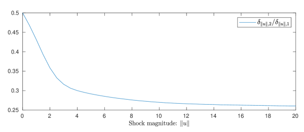
Figure 6.1: Directions of shocks having only transitory effects

6.1 illustrates this is indeed the case for a bivariate ($p=2$) model with

$$\tilde{\alpha} =-\begin{bmatrix}1\\ 0.5\end{bmatrix} \alpha =-\begin{bmatrix}1\\ 0.25\end{bmatrix} \beta =\begin{bmatrix}1\\ -1\end{bmatrix},$$

and $\Lambda(\xi)=2\lvert\Phi(\xi)-0.5\rvert$. (Without loss of generality, we take $\mathfrak{z}=0$.) For each $\lVert u\rVert$ between $0$ and $10$, the figure reports the (unique) direction $\delta_{\lVert u\rVert}$ such that $u_{\tau}=\lVert u\rVert\delta_{\lVert u\rVert}$ has no permanent effect on $z_{t}$; for the sake of comparability with $\tilde{\alpha}$ and $\alpha$, both of which have unit first element, this is reported in terms of the ratio $\delta_{\lVert u\rVert,2}/\delta_{\lVert u\rVert,1}$. We see here that $\delta_{\lVert u\rVert,2}/\delta_{\lVert u\rVert,1}$ takes the value $0.5=\tilde{\alpha}_{2}$ when $\lVert u\rVert=0$, and tends towards $0.25=\alpha_{1}$ as $\lVert u\rVert$ grows (equalling $0.26$ when $\lVert u\rVert=20$). As a consequence

$$\bigcap_{u\in\mathbb{R}^{p}}\operatorname{sp}\delta_{\lVert u\rVert}=\emptyset,$$

and as such there is no direction along which the reduced form shocks $u_{t}$ will only have transient effects. There is thus no possibility of discriminating between the underlying structural shocks $\varepsilon_{t}$ according to whether not they have permanent effects: each must, depending on the magnitude of the shock.

7 Piecewise affine VARs

Finally, we introduce a class of regime-switching models in which the conditions required for our results may be verified relatively straightforwardly. Suppose that for each $i\in\{0,\ldots,k\}$,

$$f_{i}(z)=\sum_{\ell=1}^{L}\mathbf{1}\{z\in\mathscr{Z}^{(\ell)}\}(\bar{\phi}_{i}^{(\ell)}+\Phi_{i}^{(\ell)}z),$$ (7.1)

where $\{\mathscr{Z}^{(\ell)}\}_{\ell=1}^{L}$ is a collection of convex sets that partition $\mathbb{R}^{p}$, $\{\bar{\phi}_{i}^{(\ell)}\}_{\ell=1}^{L}\subset\mathbb{R}^{p}$ and $\{\Phi_{i}^{(\ell)}\}_{\ell=1}^{L}\subset\mathbb{R}^{p\times p}$. When these parameters are such that $f_{i}$ is continuous for each $i\in\{0,\ldots,k\}$, we shall say that each $f_{i}$ is a piecewise affine function, and refer to the model as a piecewise affine VAR. (We do not consider cases in which $f_{i}$ may be discontinuous; so continuity is always implied when a function or VAR is described as being piecewise affine.)

Piecewise affine VARs, of which the CKSVAR of Mavroeidis (2021) is a recent instance, provide a flexible but tractable means of introducing nonlinearity into a vector autoregressive model. Defining

$$\mathbf{1}^{(\ell)}(z)\coloneqq\mathbf{1}\{z\in\mathscr{Z}_{i}^{(\ell)}\},$$

we see that

$$f_{0}(z_{t})-\sum_{i=1}^{k}f_{i}(z_{t-i})=\sum_{\ell=1}^{L}\mathbf{1}^{(\ell)}(z_{t})(\bar{\phi}_{i}^{(\ell)}+\Phi_{i}^{(\ell)}z_{t})-\sum_{i=1}^{k}\sum_{\ell=1}^{L}\mathbf{1}^{(\ell)}(z_{t-i})(\bar{\phi}_{i}^{(\ell)}+\Phi_{i}^{(\ell)}z_{t-i}).$$

This is a kind of endogenous regime-switching VAR, in which the sets $\{\mathscr{Z}^{(\ell)}\}_{\ell=1}^{L}$ demarcate $L$ distinct ‘regimes’. However, unlike in typical models of this kind, there is no requirement that the same ‘regime’ apply e.g. to $z_{t}$ and $z_{t-1}$ – each may lie in a different member of $\{\mathscr{Z}^{(\ell)}\}_{\ell=1}^{L}$ – and so it might be more correct to say that there are a total of $L^{k}$ autoregressive regimes, once all the possible patterns of membership of $\{z_{t-i}\}_{i=0}^{k}$ in the sets $\{\mathscr{Z}^{(\ell)}\}_{\ell=1}^{L}$ are allowed for. Nonetheless, it turns out that a fruitful approach to analysing the long-run behaviour of these systems focuses attention on those $L$ ‘linear submodels’ that arise when each of $\{z_{t-i}\}_{i=0}^{k}$ lie in the same $\mathscr{Z}^{(\ell)}$, to each $\ell\in\{1,\ldots,L\}$ of which we may associate the autoregressive polynomial

$$\Phi^{(\ell)}(\lambda)\coloneqq\Phi_{0}^{(\ell)}-\sum_{i=1}^{k}\Phi_{i}^{(\ell)}\lambda^{i}.$$ (7.2)

7.1 Simplification of the JSR condition

The conditions for membership of ${\cal M}_{r}$, for piecewise affine VARs, will parallel (i)–3. Before stating these, we first give a result that reduces (iii) to a condition on the JSR of a collection of only $L$ matrices (rather than a collection of uncountably many matrices). To state it, observe that

$$\pi(z) =-\sum_{\ell=1}^{L}\mathbf{1}^{(\ell)}(z)\left[\left(\bar{\phi}_{0}^{(\ell)}-\sum_{i=1}^{k}\bar{\phi}_{i}^{(\ell)}\right)+\left(\Phi_{0}^{(\ell)}-\sum_{i=1}^{k}\Phi_{i}^{(\ell)}\right)z\right]$$

$$\eqqcolon\sum_{\ell=1}^{L}\mathbf{1}^{(\ell)}(z)(\bar{\pi}^{(\ell)}+\Pi^{(\ell)}z).$$ (7.3)

In this context, we note that (ii) effectively requires that

$$\Pi^{(\ell)}=-\Phi^{(\ell)}(1)=\alpha\beta^{(\ell)\mathsf{T}}$$ (7.4)

where $\alpha,\beta^{(\ell)}\in\mathbb{R}^{p\times r}$ with $\operatorname{rk}\alpha=\operatorname{rk}\beta^{(\ell)}=r$. Further, let $\Gamma_{j}^{(\ell)}\coloneqq-\sum_{j=i+1}^{k}\Phi_{j}^{(\ell)}$, $\boldsymbol{\Gamma}^{(\ell)}\coloneqq[\Gamma_{i}^{(\ell)}]_{i=1}^{k-1}$, and

$$\boldsymbol{\beta}^{(\ell)\mathsf{T}} \coloneqq\begin{bmatrix}\beta^{(\ell)\mathsf{T}}(\Phi_{0}^{(\ell)})^{-1}&0\\ \boldsymbol{\Gamma}^{(\ell)}(\Phi_{0}^{(\ell)})^{-1}&D\end{bmatrix} \boldsymbol{\alpha} \coloneqq\begin{bmatrix}\alpha&E^{\mathsf{T}}\\ 0&I_{p(k-1)}\end{bmatrix}.$$ (7.5)

Lemma 7.1.

Suppose that $(c,\{f_{i}\}_{i=0}^{k})$ is a piecewise affine model, for which there exists an $\alpha\in\mathbb{R}^{p\times r}$ with $\operatorname{rk}\alpha=r$ such that

1. $c=\alpha\mu$, $\bar{\pi}^{(\ell)}=\alpha\bar{\mu}^{(\ell)}$ and $\Pi^{(\ell)}=\alpha\beta^{(\ell)\mathsf{T}}$, for $\mu,\bar{\mu}^{(\ell)},\beta^{(\ell)}\in\mathbb{R}^{p\times r}$, for all $\ell\in\{1,\ldots,L\}$; and

2. $f_{0}:\mathbb{R}^{p}\rightarrow\mathbb{R}^{p}$ is a homeomorphism.

Then $(c,\{f_{i}\}_{i=0}^{k})$ satisfies (LABEL:gradient) with ${\cal B}$ equal to $\operatorname{co}\{\boldsymbol{\beta}^{(\ell)}\}_{\ell=1}^{L}$, and so

$$\rho_{{\scriptstyle\mathrm{JSR}}}(\{I_{p(k-1)+r}+\boldsymbol{\beta}^{\mathsf{T}}\boldsymbol{\alpha}\mid\boldsymbol{\beta}\in{\cal B}\})=\rho_{{\scriptstyle\mathrm{JSR}}}(\{I_{p(k-1)+r}+\boldsymbol{\beta}^{(\ell)\mathsf{T}}\boldsymbol{\alpha}\}_{\ell=1}^{L}).$$

Since the $p(k-1)+r$ eigenvalues of $I_{p(k-1)+r}+\boldsymbol{\beta}^{(\ell)\mathsf{T}}\boldsymbol{\alpha}$ correspond to the inverses of the non-unit roots of $\Phi^{(\ell)}(\lambda)$, a necessary, though not sufficient condition for

$$\rho_{{\scriptstyle\mathrm{JSR}}}(\{I_{p(k-1)+r}+\boldsymbol{\beta}^{(\ell)\mathsf{T}}\boldsymbol{\alpha}\}_{\ell=1}^{L})<1$$

is that the eigenvalues of $I_{p(k-1)+r}+\boldsymbol{\beta}^{(\ell)\mathsf{T}}\boldsymbol{\alpha}$ should lie strictly inside the unit circle, for all $\ell\in\{1,\ldots,L\}$. Thus, if $\operatorname{rk}\Phi^{(\ell)}(1)=q=p-r$, as per (LABEL:Pi-ell), then $\Phi^{(\ell)}(\lambda)$ will have $q$ roots at unity, and all others strictly outside the unit circle (this follows e.g. from arguments given in the proof of 2.1). In other words, for a piecewise affine model to belong to class ${\cal M}_{r}(\alpha,\overline{b},\overline{\rho})$ (for some $\overline{\rho}<1$), it is essentially necessary that each of its $L$ linear submodels satisfy the usual conditions for a linear VAR to give rise to $q$ common trends and $r$ cointegrating relations (i.e. conditions (ii) and (iii) above).

7.2 Membership of ${\cal M}_{r}$

It remains to consider (i), i.e. the requirement that $f_{0}$ be a homeomorphism. For the purposes of verifying this condition, two important special cases of the piecewise affine VAR are:

• the piecewise linear VAR (PLVAR), in which there exists a basis $\{a_{i}\}_{i=1}^{p}$ for $\mathbb{R}^{p}$ such that each $\mathscr{Z}^{(\ell)}$ can be written as a union of cones of the form

  $$\mathscr{C}_{{\cal I}}\coloneqq\{z\in\mathbb{R}^{p}\mid a_{i}^{\mathsf{T}}z\geq 0,\ \forall i\in{\cal I}\text{ and }a_{i}^{\mathsf{T}}z<0,\ \forall i\notin{\cal I}\}$$

  where ${\cal I}$ ranges over the subsets of $\{1,\ldots,p\}$, and $\bar{\phi}_{i}^{(\ell)}=0$ for all $i$ and $\ell$; and

• the threshold affine VAR (TAVAR), in which there exists an $a\in\mathbb{R}^{p}\backslash\{0\}$ and thresholds $\{\tau_{\ell}\}_{\ell=0}^{L}$ with $\tau_{\ell}<\tau_{\ell+1}$, $\tau_{0}=-\infty$ and $\tau_{L}=+\infty$, such that

  $$\mathscr{Z}^{(\ell)}=\{z\in\mathbb{R}^{p}\mid a^{\mathsf{T}}z\in(\tau_{\ell-1},\tau_{\ell}]\},$$

  i.e. the sets $\{\mathscr{Z}^{(\ell)}\}$ take the forms of ‘bands’ in $\mathbb{R}^{p}$. (In typical examples, $a=e_{p,i}$, i.e. it picks out one ‘threshold variable’ from the elements of $z_{t}$.)

In these models, the results of Gourieroux et al. (1980) provide necessary and sufficient conditions for $f_{0}$ to be invertible, which can be expressed in terms of the determinants of $\{\Phi_{0}^{(\ell)}\}_{\ell=1}^{L}$. We thus have the following

Proposition 7.1.

Suppose is $(c,\{f_{i}\}_{i=0}^{k})$ is either a piecewise linear or threshold affine VAR, such that:

1. $\operatorname{sgn}\det\Phi_{0}^{(\ell)}=\operatorname{sgn}\det\Phi_{0}^{(1)}\neq 0$ for all $\ell\in\{1,\ldots,L\}$;

2. $c=\alpha\mu$, $\bar{\pi}^{(\ell)}=\alpha\bar{\mu}^{(\ell)}$ , and $\Pi^{(\ell)}=\alpha\beta^{(\ell)\mathsf{T}}$, where $\alpha,\beta^{(\ell)}\in\mathbb{R}^{p\times r}$ have rank $r$, for all $\ell\in\{1,\ldots,L\}$; and

3. $\rho_{{\scriptstyle\mathrm{JSR}}}(\{I_{p(k-1)+r}+\boldsymbol{\beta}^{(\ell)\mathsf{T}}\boldsymbol{\alpha}\}_{\ell=1}^{L})\leq\overline{\rho}$.

Then $(c,\{f_{i}\}_{i=0}^{k})$ belongs to class ${\cal M}_{r}(\alpha,\overline{b},\overline{\rho})$, for $\overline{b}\geq\max_{1\leq\ell\leq L}\lVert\boldsymbol{\beta}^{(\ell)}\rVert$, with

$$\chi(z)=\begin{bmatrix}\psi(z)\\ \theta(z)\end{bmatrix}=\sum_{\ell=1}^{L}\mathbf{1}^{(\ell)}(z)\left\{\begin{bmatrix}\alpha_{\perp}^{\mathsf{T}}\bar{\psi}^{(\ell)}\\ \bar{\mu}^{(\ell)}\end{bmatrix}+\begin{bmatrix}\alpha_{\perp}^{\mathsf{T}}\mathrm{H}^{(\ell)}\\ \beta^{(\ell)\mathsf{T}}\end{bmatrix}z\right\}\eqqcolon\sum_{\ell=1}^{L}\mathbf{1}^{(\ell)}(z)\{\bar{\chi}^{(\ell)}+\mathrm{X}^{(\ell)}z\}$$ (7.6)

where

$$\bar{\psi}^{(\ell)} \coloneqq\bar{\phi}_{0}^{(\ell)}-\sum_{i=1}^{k-1}\bar{\gamma}_{i}^{(\ell)} \mathrm{H}^{(\ell)} \coloneqq\Phi_{0}^{(\ell)}-\sum_{i=1}^{k-1}\Gamma_{i}^{(\ell)}$$

for $\bar{\gamma}_{i}^{(\ell)}\coloneqq-\sum_{j=i+1}^{k}\bar{\phi}_{j}^{(\ell)}$. Moreover, the same conclusion holds if $(c,\{f_{i}\}_{i=0}^{k})$ is a general piecewise affine model satisfying (ii) and (iii) above, if $f_{0}$ is a homeomorphism.

Since it may be verified that a linear VAR satisfying (i)–3 is itself a piecewise linear model satisfying (i)–3 above, 2.1 may be construed as a special case of the preceding (though for expository reasons, a separate proof of that result is given in D).

7.3 Smooth transitions

The model (LABEL:pwa) may also be extended to allow for smooth transitions between the $L$ regimes. In the literature on smooth transition (vector) autoregressive models, the conventional approach (e.g. Hubrich and Teräsvirta, 2013, Sec. 3.3) is to replace the indicator functions $\mathbf{1}\{z\in\mathscr{Z}^{(\ell)}\}$ by smooth maps $\Lambda^{(\ell)}(z)$, so that now

$$f_{i}^{\mathrm{ST}}(z)=\sum_{\ell=1}^{L}\Lambda^{(\ell)}(z)(\bar{\phi}_{i}^{(\ell)}+\Phi_{i}^{(\ell)}z),$$

where $\Lambda^{(\ell)}(z)\in[0,1]$ and $\sum_{\ell=1}^{L}\Lambda^{(\ell)}(z)=1$ for all $z\in\mathbb{R}^{p}$, so that $f_{i}^{\mathrm{ST}}(z)$ is a always a smooth, convex combination of the affine functions $\{z\mapsto\bar{\phi}_{i}^{(\ell)}+\Phi_{i}^{(\ell)}z\}_{\ell=1}^{L}$. While models of this kind may be accommodated within our framework (under certain regularity conditions), the fact that the gradient of $f_{i}^{\mathrm{ST}}$ is not a convex combination of those underlying affine regimes makes it difficult to reduce (iii) to a bound on the JSR of a finite collection of matrices, in the manner of 7.1. As an alternative specification that allows for smooth transitions between regimes, while also keeping (iii) tractable, consider

$$f_{i,K}(z)\coloneqq\int_{\mathbb{R}^{p}}f_{i}(z+u)K(u)\,\mathrm{d}u$$ (7.7)

where $f_{i}$ is a (continuous) piecewise affine function as in (LABEL:pwa) above, and $K$ is a smooth kernel with mean zero. Then we have the following.

Proposition 7.2.

Suppose that:

1. $(c,\{f_{i}\}_{i=0}^{k})$ is either a piecewise linear or threshold affine VAR satisfying (i)–3;

2. $\Phi_{0}^{(\ell)}=\Phi_{0}$ for all $\ell\in\{1,\ldots,L\}$, for some nonsingular $\Phi_{0}$;

3. $K:\mathbb{R}\rightarrow\mathbb{R}$ is continuous and non-negative, with $\int_{\mathbb{R}^{p}}K(u)\,\mathrm{d}u=1$ and $\int_{\mathbb{R}^{p}}uK(u)\,\mathrm{d}u=0$;

4. $f_{i,K}$ is constructed by smoothing $f_{i}$ with $K$ as in (LABEL:smoothed), for $i\in\{0,\ldots,k\}$.

Then $(c,\{f_{i,K}\}_{i=0}^{k})$ belongs to class ${\cal M}_{r}(\alpha,\overline{b},\overline{\rho})$, for $\overline{b}\geq\max_{1\leq\ell\leq L}\lVert\boldsymbol{\beta}^{(\ell)}\rVert$, for $\boldsymbol{\beta}^{(\ell)}$ as in (LABEL:beta_l) above.

The requirement in (ii) that $f_{0}$ be linear is needed principally to facilitate the verification of (iii), because of the role played by $f_{K,0}^{-1}$ there. We expect that it should be possible to extend the preceding to allow $f_{0}$ to be a general piecewise affine function, albeit possibly at the cost of additional regularity conditions. (Indeed, it may be shown that the smooth counterpart $f_{0,K}$ of $f_{0}$ is a homeomorphism if every $\Phi\in\operatorname{co}\{\Phi_{0}^{(\ell)}\}_{\ell=1}^{L}$ is invertible, thereby satisfying (i).)

8 Conclusion

This paper has extended the Granger–Johansen representation theorem to a flexible class of additively time-separable, nonlinear SVAR models. This shows that such models may be applied directly to time series in which (common) stochastic trends are present, without the need for pre-filtering, thus avoiding the potential for misspecification that this entails. As an important corollary to our results, we show that these models are capable of supporting the same kinds of long-run identifying restrictions as are available in linear cointegrated SVARs. A companion paper to the present work provides limit theory for $n^{-1/2}z_{\lfloor n\lambda\rfloor}$, and a further discussion of nonlinear cointegration, under the assumptions maintained here.

Appendix A Auxiliary lemmas

As noted in 2.12.1, we shall not generally indicate how our results may specialise in cases where $k\in\{1,2\}$; the reader is accordingly advised to treat these models as particular degenerate instances of the VAR($k$) model with $k\geq 3$.

Lemma A.1.

Suppose $f:\mathbb{R}^{d_{x}}\rightarrow\mathbb{R}^{d_{y}}$. Then the following are equivalent:

1. $f$ is Lipschitz, with Lipschitz constant $K$;

2. for every $x,x^{\prime}\in\mathbb{R}^{d_{x}}$, there exists a $\beta\in\mathbb{R}^{d_{x}\times d_{y}}$ with $\lVert\beta\rVert\leq K$ such that

   $$f(x)-f(x^{\prime})=\beta^{\mathsf{T}}(x-x^{\prime})$$ (A.1)

Recall the definitions of $\{g_{i}\}_{i=0}^{k-1}$, $\pi$ and $\chi$ given in (LABEL:ge), (LABEL:pi-def) and (LABEL:co-map).

Lemma A.2.

Suppose $(c,\{f_{i}\}_{i=0}^{k})$ belongs to class ${\cal M}_{r}(\alpha,\overline{b},\overline{\rho})$. Then the model $(c^{\ast},\{f_{i}^{\ast}\}_{i=0}^{k})$, with $c^{\ast}=c$ and $f_{i}^{\ast}=f_{i}\circ f_{0}^{-1}$ for $i\in\{0,\ldots,k\}$ belongs to class ${\cal M}_{r}^{\ast}(\alpha,\overline{b},\overline{\rho})$, with $g_{i}^{\ast}=g_{i}\circ f_{0}^{-1}$ for $i\in\{0,\ldots,k-1\}$, $\pi^{\ast}=\pi\circ f_{0}^{-1}$, and

$$\chi^{\ast}=\begin{bmatrix}\psi^{\ast}\\ \theta^{\ast}\end{bmatrix}=\begin{bmatrix}\psi\circ f_{0}^{-1}\\ \theta\circ f_{0}^{-1}\end{bmatrix}=\chi\circ f_{0}^{-1}.$$

Moreover, we may take ${\cal B^{\ast}}={\cal B}$, where ${\cal B}$ and ${\cal B}^{\ast}$ satisfy (iii) for models $(c,\{f_{i}\}_{i=0}^{k})$ and $(c^{\ast},\{f_{i}^{\ast}\}_{i=0}^{k})$ respectively.

Recall the definition of $\boldsymbol{\alpha}_{\perp}$ from (LABEL:bold-alpha).

Lemma A.3.

Let $\alpha\in\mathbb{R}^{p\times r}$ with $\operatorname{rk}\alpha=r$, $\overline{b}<\infty$ and $\overline{\rho}<1$. Then

$$\sup_{\boldsymbol{\beta}\in{\cal B}}\left\|\begin{bmatrix}\boldsymbol{\alpha}_{\perp}^{\mathsf{T}}\\ \boldsymbol{\beta}^{\mathsf{T}}\end{bmatrix}^{-1}\right\|<\infty$$

Recall the definition of a bi-Lipschitz function given in 2.3.

Lemma A.4.

Suppose $(c,\{f_{i}\}_{i=0}^{k}\}$ belongs to class ${\cal M}_{r}(\alpha,\overline{b},\overline{\rho})$, for some $\overline{b}<\infty$ and $\overline{\rho}<1$. Then $f_{i}$ is continuous for $i\in\{1,\ldots,k-1\}$, and the map $\chi:\mathbb{R}^{p}\rightarrow\mathbb{R}^{p}$ in (LABEL:co-map) is a homeomorphism. If in addition $f_{0}$ is bi-Lipschitz, with bi-Lipschitz constant $C_{f_{0}}$, then $\chi$ is also bi-Lipschitz, with bi-Lipschitz constant that depends only on $\alpha$, $\overline{b}$, $\overline{\rho}$ and $C_{f_{0}}$.

Appendix B Proofs of auxiliary lemmas

Since some of the proofs rely on the representation given in 2.1, the proof of this result is given first.

Proof of 2.1.

By direct calculation,

$$\sum_{i=1}^{k}f_{i}(z_{t-i})+g_{0}(z_{t-1}) =-\sum_{i=1}^{k}[f_{i}(z_{t-1})-f_{i}(z_{t-i})]$$

$$=-\sum_{i=1}^{k}\sum_{j=1}^{i-1}\Delta f_{i}(z_{t-j})=-\sum_{j=1}^{k-1}\sum_{i=j+1}^{k}\Delta f_{i}(z_{t-j})$$

$$=\sum_{j=1}^{k-1}\Delta\left[-\sum_{i=j+1}^{k}f_{i}(z_{t-j})\right]=\sum_{j=1}^{k-1}\Delta g_{j}(z_{t-j}),$$

whence it follows from (LABEL:nlVAR) and the definition of $\pi(z)$ that

$$\Delta f_{0}(z_{t}) =c-f_{0}(z_{t-1})+\sum_{i=1}^{k}f_{i}(z_{t-i})+u_{t}$$

$$=c-[f_{0}(z_{t-1})+g_{0}(z_{t-1})]+\sum_{i=1}^{k-1}\Delta g_{i}(z_{t-i})+u_{t}$$

$$=c+\pi(z_{t-1})+\sum_{i=1}^{k-1}\Delta g_{i}(z_{t-i})+u_{t}$$

which yields (LABEL:VECM-first). Further, since $\zeta_{j,t}=\sum_{i=j}^{k-1}g_{i}(z_{t-i+j})$,

$$\sum_{i=1}^{k-1}\Delta g_{i}(z_{t-i}) =\sum_{i=1}^{k-1}g_{i}(z_{t-i})-\sum_{i=1}^{k-1}g_{i}(z_{t-1-i})$$

$$=g_{1}(z_{t-1})+\sum_{i=2}^{k-1}g_{i}(z_{t-i})-\sum_{i=1}^{k-1}g_{i}(z_{t-1-i})$$

$$=g_{1}(z_{t-1})-\sum_{i=1}^{k-1}g_{i}(z_{(t-2)-i+1})+\sum_{i=2}^{k-1}g_{i}(z_{(t-2)-i+2})$$

$$=g_{1}(z_{t-1})-\zeta_{1,t-2}+\zeta_{2,t-2}=g_{1}(z_{t-1})+D_{1}\boldsymbol{\zeta}_{t-2}$$

so that

$$\Delta f_{0}(z_{t})=c+[\pi(z_{t-1})+g_{1}(z_{t-1})]+D_{1}\boldsymbol{\zeta}_{t-2}+u_{t}$$

as per the first $p$ elements of (LABEL:VECM-system). Finally, we note that for $j\in\{1,\ldots,k-2\}$,

$$\Delta\zeta_{j,t-1} =\zeta_{j,t-1}-\zeta_{j,t-2}=\sum_{i=j}^{k-1}g_{i}(z_{(t-1)-i+j})-\zeta_{j,t-2}$$

$$=g_{j}(z_{t-1})+\sum_{i=j+1}^{k-1}g_{i}(z_{(t-1)-i+j})-\zeta_{j,t-2}$$

$$=g_{j}(z_{t-1})+\sum_{i=j+1}^{k-1}g_{i}(z_{(t-2)-i+(j+1)})-\zeta_{j,t-2}$$

$$=g_{j}(z_{t-1})-\zeta_{j,t-2}+\zeta_{j+1,t-2}$$

and

$$\Delta\zeta_{k-1,t-1}=g_{k-1}(z_{t-1})-\zeta_{k-1,t-2},$$

so that stacking these equations as $j$ ranges over $\{1,\ldots,k-1\}$ yields the remaining elements of (LABEL:VECM-system). ∎

Proof of A.1.

(ii) trivially implies (i); it remains to prove the reverse implication. Let $x,x^{\prime}\in\mathbb{R}^{d_{y}}$ with $x\neq x^{\prime}$ be given, and let $\delta_{x}\coloneqq x-x^{\prime}\neq 0$ and $\delta_{f}\coloneqq f(x)-f(x^{\prime})$, so that $\lVert\delta_{f}\rVert\leq K\lVert\delta_{x}\rVert$ by (i). Taking $\beta^{\mathsf{T}}\coloneqq\delta_{f}(\delta_{x}^{\mathsf{T}}\delta_{x})^{-1}\delta_{x}^{\mathsf{T}}$ satisfies (LABEL:f-x). Finally, we note

$$\lVert\beta^{\mathsf{T}}\rVert=\lVert\beta\rVert=\sup_{\lVert z\rVert=1}\lVert\delta_{f}(\delta_{x}^{\mathsf{T}}\delta_{x})^{-1}\delta_{x}^{\mathsf{T}}z\rVert=\lVert\delta_{f}\rVert\lvert\delta_{x}^{\mathsf{T}}\delta_{x}\rvert^{-1}\sup_{\lVert z\rVert=1}\lvert\delta_{x}^{\mathsf{T}}z\rvert=_{(1)}\lVert\delta_{f}\rVert/\lVert\delta_{x}\rVert\leq K,$$

where $=_{(1)}$ holds because the maximum is achieved by taking $z=\delta_{x}/\lVert\delta_{x}\rVert$. ∎

Proof of A.2.

The claimed forms of $\{g_{i}^{\ast}\}_{i=1}^{k-1}$, $\pi^{\ast}$ and $\chi^{\ast}$ follow immediately from the definitions of these objects, e.g. from (LABEL:ge) we have

$$g_{j}^{\ast}=-\sum_{i=j+1}^{k}f_{i}^{\ast}=-\sum_{i=j+1}^{k}f_{i}\circ f_{0}^{-1}=\left(-\sum_{i=j+1}^{k}f_{i}\right)\circ f_{0}^{-1}=g_{j}\circ f_{0}^{-1},$$

etc. It remains to verify the three conditions required for $(c^{\ast},\{f_{i}^{\ast}\}_{i=0}^{k})$ to belong to class ${\cal M}_{r}^{\ast}(\alpha,\overline{b},\overline{\rho})$, as per 2.1.

(i). $f_{0}^{\ast}$ is the identity by construction, and thus trivially a homeomorphism.

(ii). Holds trivially since $c^{\ast}=c=\alpha\mu$ and

$$\pi^{\ast}(z)=\pi[f_{0}^{-1}(z)]=\alpha\theta[f_{0}^{-1}(z)]=\alpha\theta^{\ast}(z).$$

It follows, moreover, that $\alpha^{\ast}=\alpha$.

(iii). We have $\boldsymbol{\theta}^{\ast}\circ(f_{0}^{\ast})^{-1}=\boldsymbol{\theta}^{\ast}=\boldsymbol{\theta}\circ f_{0}^{-1}$, and so

$$[\boldsymbol{\theta}^{\ast}\circ(f_{0}^{\ast})^{-1}](z)+\boldsymbol{D}_{0}\boldsymbol{z}=(\boldsymbol{\theta}\circ f_{0}^{-1})(z)+\boldsymbol{D}_{0}\boldsymbol{z}$$

for every $\boldsymbol{z}=(z^{\mathsf{T}},\boldsymbol{\zeta}^{\mathsf{T}})^{\mathsf{T}}\in\mathbb{R}^{kp}$. Since the r.h.s. satisfies (LABEL:gradient), and $\alpha^{\ast}=\alpha$, we may deduce that (iii) holds for $(c^{\ast},\{f_{i}^{\ast}\}_{i=0}^{k})$ with the same ${\cal B}$, $\overline{b}$ and $\overline{\rho}$ as for $(c,\{f_{i}\}_{i=0}^{k})$. ∎

Proof of A.3.

Let $\delta>0$ be such that $\overline{\rho}+\delta<1$, and ${\cal B}\in{\cal M}_{r}(\alpha,\overline{b},\overline{\rho})$. For any $\boldsymbol{\beta}\in{\cal B}$,

$$\begin{bmatrix}\boldsymbol{\alpha}_{\perp}^{\mathsf{T}}\\ \boldsymbol{\beta}^{\mathsf{T}}\end{bmatrix}=\begin{bmatrix}I_{r}&0\\ \boldsymbol{\beta}^{\mathsf{T}}\boldsymbol{\alpha}_{\perp}(\boldsymbol{\alpha}_{\perp}^{\mathsf{T}}\boldsymbol{\alpha}_{\perp})^{-1}&\boldsymbol{\beta}^{\mathsf{T}}\boldsymbol{\alpha}\end{bmatrix}\begin{bmatrix}\boldsymbol{\alpha}_{\perp}^{\mathsf{T}}\\ (\boldsymbol{\alpha}^{\mathsf{T}}\boldsymbol{\alpha})^{-1}\boldsymbol{\alpha}^{\mathsf{T}}\end{bmatrix},$$

where $\boldsymbol{\alpha}$ and $\boldsymbol{\alpha}_{\perp}$ are as defined in (LABEL:bold-alpha). By construction, $\boldsymbol{\alpha}\in\mathbb{R}^{kp\times[p(k-1)+r]}$ and $\boldsymbol{\alpha}_{\perp}\in\mathbb{R}^{kp\times q}$ have full column rank, and $\boldsymbol{\alpha}_{\perp}^{\mathsf{T}}\boldsymbol{\alpha}=0$. They thus span the whole of $\mathbb{R}^{kp}$, whence the second r.h.s. matrix is invertible. It will be shown below that $\boldsymbol{\beta}^{\mathsf{T}}\boldsymbol{\alpha}$ is invertible, and hence so too is the first r.h.s. matrix. Therefore

$$\begin{bmatrix}\boldsymbol{\alpha}_{\perp}^{\mathsf{T}}\\ \boldsymbol{\beta}^{\mathsf{T}}\end{bmatrix}^{-1} =\begin{bmatrix}\boldsymbol{\alpha}_{\perp}^{\mathsf{T}}\\ (\boldsymbol{\alpha}^{\mathsf{T}}\boldsymbol{\alpha})^{-1}\boldsymbol{\alpha}^{\mathsf{T}}\end{bmatrix}^{-1}\begin{bmatrix}I_{r}&0\\ -(\boldsymbol{\beta}^{\mathsf{T}}\boldsymbol{\alpha})^{-1}\boldsymbol{\beta}^{\mathsf{T}}\boldsymbol{\alpha}_{\perp}(\boldsymbol{\alpha}_{\perp}^{\mathsf{T}}\boldsymbol{\alpha}_{\perp})^{-1}&(\boldsymbol{\beta}^{\mathsf{T}}\boldsymbol{\alpha})^{-1}\end{bmatrix}$$

$$=\begin{bmatrix}\boldsymbol{\alpha}_{\perp}^{\mathsf{T}}\\ (\boldsymbol{\alpha}^{\mathsf{T}}\boldsymbol{\alpha})^{-1}\boldsymbol{\alpha}^{\mathsf{T}}\end{bmatrix}^{-1}\begin{bmatrix}I_{r}&0\\ 0&(\boldsymbol{\beta}^{\mathsf{T}}\boldsymbol{\alpha})^{-1}\end{bmatrix}\begin{bmatrix}I_{r}&0\\ -\boldsymbol{\beta}^{\mathsf{T}}\boldsymbol{\alpha}_{\perp}(\boldsymbol{\alpha}_{\perp}^{\mathsf{T}}\boldsymbol{\alpha}_{\perp})^{-1}&I_{p(k-1)}\end{bmatrix}$$

$$\eqqcolon M_{1}M_{2}(\boldsymbol{\beta})M_{3}(\boldsymbol{\beta}).$$

Let $\overline{B}(0,\overline{b})$ denote the closed ball centred at zero, of radius $\overline{b}$, in $\mathbb{R}^{pk\times[p(k-1)+r]}$, and

$${\cal K}\coloneqq\{I_{p(k-1)+r}+\boldsymbol{\beta}^{\mathsf{T}}\boldsymbol{\alpha}\mid\boldsymbol{\beta}\in\overline{B}(0,\overline{b})\}.$$

Then $\{I_{p(k-1)+r}+\boldsymbol{\beta}^{\mathsf{T}}\boldsymbol{\alpha}\mid\boldsymbol{\beta}\in{\cal B}\}$ is a closed subset of ${\cal K}$. Suppose that ${\cal B}\subset\mathbb{R}^{m\times m}$ is compact, with $\rho_{{\scriptstyle\mathrm{JSR}}}({\cal B})\leq\overline{\rho}$. It follows by Jungers (2009, Prop. 1.4) that that there exists a norm $\lVert\cdot\rVert_{\delta}$ on $\mathbb{R}^{p(k-1)+r}$ such that

$$\max_{\boldsymbol{\beta}\in{\cal B}}\lVert I_{p(k-1)+r}+\boldsymbol{\beta}^{\mathsf{T}}\boldsymbol{\alpha}\rVert_{\delta}\leq\overline{\rho}+\delta<1.$$

Hence, by the equivalence of $\lVert\cdot\rVert_{\delta}$ and $\lVert\cdot\rVert$, there exists a $C_{0}<\infty$ such that for all $\boldsymbol{\beta}\in{\cal B}$,

$$\lVert(\boldsymbol{\beta}^{\mathsf{T}}\boldsymbol{\alpha})^{-1}\rVert\leq_{(1)}C_{0}\lVert(\boldsymbol{\beta}^{\mathsf{T}}\boldsymbol{\alpha})^{-1}\rVert_{\delta}=C_{0}\left\|\sum_{k=0}^{\infty}(I+\boldsymbol{\beta}^{\mathsf{T}}\boldsymbol{\alpha})^{k}\right\|_{\delta}\\ \leq C_{0}\sum_{k=0}^{\infty}\lVert I+\boldsymbol{\beta}^{\mathsf{T}}\boldsymbol{\alpha}\rVert_{\delta}^{k}\leq\frac{C_{0}}{1-(\overline{\rho}+\delta)}<\infty,$$

where $\leq_{(1)}$ holds by Theorem 5.6.18 in Horn and Johnson (2013). Thus $\boldsymbol{\beta}^{\mathsf{T}}\boldsymbol{\alpha}$ is indeed invertible as claimed. Since the final bound is independent of ${\cal B}$, it follows that

$$\sup_{\boldsymbol{\beta}\in{\cal B}}\lVert M_{2}(\boldsymbol{\beta})\rVert<\infty,$$

while also

$$\sup_{\boldsymbol{\beta}\in{\cal B}}\lVert M_{3}(\boldsymbol{\beta})\rVert\leq\sup_{\boldsymbol{\beta}\in\overline{B}(0,\overline{b})}\lVert M_{3}(\boldsymbol{\beta})\rVert<\infty.$$

Since $M_{1}$ does not depend on $\boldsymbol{\beta}$, the claim follows. ∎

Proof of A.4.

We first suppose that $f_{0}=I_{p}$, i.e. the model is in class ${\cal M}_{r}^{\ast}(\alpha,\overline{b},\overline{\rho})$. We shall show in this case that each $\{f_{i}\}_{i=1}^{k}$ is Lipschitz; and that $\chi:\mathbb{R}^{p}\rightarrow\mathbb{R}^{p}$ is bi-Lipschitz, and therefore a homeomorphism.

To that end, define $\boldsymbol{\chi}:\mathbb{R}^{kp}\rightarrow\mathbb{R}^{kp}$ as

$$\boldsymbol{\chi}(\boldsymbol{z})\coloneqq\begin{bmatrix}\boldsymbol{\alpha}_{\perp}^{\mathsf{T}}\boldsymbol{z}\\ \boldsymbol{\theta}(z)+\boldsymbol{D}_{0}\boldsymbol{z}\end{bmatrix}=\begin{bmatrix}\alpha_{\perp}^{\mathsf{T}}[z-E^{\mathsf{T}}\boldsymbol{\zeta}]\\ \theta(z)\\ \boldsymbol{g}(z)+D\boldsymbol{\zeta}\end{bmatrix}$$ (B.1)

where $\boldsymbol{z}=(z^{\mathsf{T}},\boldsymbol{\zeta}^{\mathsf{T}})^{\mathsf{T}}$ for $z\in\mathbb{R}^{p}$ and $\boldsymbol{\zeta}\in\mathbb{R}^{p(k-1)}$. By evaluating (LABEL:bold-chi) when $\boldsymbol{\zeta}=0$, and applying A.1, we see that (iii) implies that $\theta$ and $\boldsymbol{g}$ are Lipschitz, with Lipschitz constant depending only on $\overline{b}$. Hence $g_{i}$ is Lipschitz for $i\in\{1,\ldots,k-1\}$, and moreover so too is

$$g_{0}(z)=-\pi(z)-f_{0}(z)=-\alpha\theta(z)-z.$$

Since $f_{i}=g_{i}-g_{i-1}$ by (LABEL:ge), it follows that $f_{i}$ is Lipschitz for $i\in\{1,\ldots,k\}$.

We now turn to $\chi$. Let $z_{0}\in\mathbb{R}^{p}$, $\boldsymbol{\zeta}_{0}\coloneqq-D^{-1}\boldsymbol{g}(z_{0})$, and $\boldsymbol{z}_{0}\coloneqq(z_{0}^{\mathsf{T}},\boldsymbol{\zeta}_{0}^{\mathsf{T}})^{\mathsf{T}}$. Then

$$E^{\mathsf{T}}\boldsymbol{\zeta}_{0}=-E^{\mathsf{T}}D^{-1}\boldsymbol{g}(z_{0})=\begin{bmatrix}I_{p}&0_{p\times p}&\cdots&0_{p\times p}\end{bmatrix}\begin{bmatrix}I_{p}&I_{p}&I_{p}&I_{p}\\ &I_{p}&I_{p}&I_{p}\\ &&\ddots&\vdots\\ &&&I_{p}\end{bmatrix}\begin{bmatrix}g_{1}(z_{0})\\ g_{2}(z_{0})\\ \vdots\\ g_{k-1}(z_{0})\end{bmatrix}=\sum_{i=1}^{k-1}g_{i}(z_{0})$$

and hence

$$\boldsymbol{\chi}(\boldsymbol{z}_{0})=\boldsymbol{\chi}(z_{0},\boldsymbol{\zeta}_{0})=\begin{bmatrix}\alpha_{\perp}^{\mathsf{T}}[z_{0}-\sum_{i=1}^{k-1}g_{i}(z_{0})]\\ \theta(z_{0})\\ 0_{p(k-1)}\end{bmatrix}=\begin{bmatrix}\psi(z_{0})\\ \theta(z_{0})\\ 0_{p(k-1)}\end{bmatrix}=\begin{bmatrix}\chi(z_{0})\\ 0_{p(k-1)}\end{bmatrix}.$$

Let $z_{1}\in\mathbb{R}^{p}$, $\boldsymbol{\zeta}_{1}\coloneqq-D^{-1}\boldsymbol{g}(z_{1})$ and $\boldsymbol{z}_{1}\coloneqq(z_{1}^{\mathsf{T}},\boldsymbol{\zeta}_{1}^{\mathsf{T}})^{\mathsf{T}}$. Then by the preceding (recalling $\lVert\cdot\rVert$ denotes the Euclidean norm),

$$\lVert\boldsymbol{\chi}(\boldsymbol{z}_{0})-\boldsymbol{\chi}(\boldsymbol{z}_{1})\rVert=\lVert\chi(z_{0})-\chi(z_{1})\rVert,$$

while by (iii) (with $f_{0}=I_{p}$), there exists a $\boldsymbol{\beta}\in{\cal B}$ such that

$$\boldsymbol{\chi}(\boldsymbol{z}_{0})-\boldsymbol{\chi}(\boldsymbol{z}_{1})=\begin{bmatrix}\boldsymbol{\alpha}_{\perp}^{\mathsf{T}}\\ \boldsymbol{\beta}^{\mathsf{T}}\end{bmatrix}(\boldsymbol{z}_{0}-\boldsymbol{z}_{1}).$$ (B.2)

Since $\lVert\boldsymbol{\beta}\rVert\leq\overline{b}$ for all $\boldsymbol{\beta}\in{\cal B}$, there exists a $C_{0}<\infty$ (depending only on $\overline{b}$) such that

$$\lVert\chi(z_{0})-\chi(z_{1})\rVert =\lVert\boldsymbol{\chi}(\boldsymbol{z}_{0})-\boldsymbol{\chi}(\boldsymbol{z}_{1})\rVert\leq C_{0}\lVert\boldsymbol{z}_{0}-\boldsymbol{z}_{1}\rVert.$$ (B.3)

As noted above, $\boldsymbol{g}$ is Lipschitz: hence there exists a $C_{1}<\infty$ (depending only on $\overline{b}$) such that

$$\lVert\boldsymbol{z}_{0}-\boldsymbol{z}_{1}\rVert=\left\|\begin{bmatrix}z_{0}-z_{1}\\ -D^{-1}[\boldsymbol{g}(z_{0})-\boldsymbol{g}(z_{1})]\end{bmatrix}\right\|\leq C_{1}\lVert z_{0}-z_{1}\rVert.$$ (B.4)

By A.3, the matrix on the r.h.s. of (LABEL:boldco) is invertible; hence

$$\lVert\boldsymbol{z}_{0}-\boldsymbol{z}_{1}\rVert\leq\left\|\begin{bmatrix}\boldsymbol{\alpha}_{\perp}^{\mathsf{T}}\\ \boldsymbol{\beta}^{\mathsf{T}}\end{bmatrix}^{-1}\right\|\lVert\boldsymbol{\chi}(\boldsymbol{z}_{0})-\boldsymbol{\chi}(\boldsymbol{z}_{1})\rVert.$$

That lemma further implies that there exists a $C_{2}<\infty$, depending only on $\alpha$, $\overline{b}$ and $\overline{\rho}$, such that

$$\lVert\chi(z_{0})-\chi(z_{1})\rVert =\lVert\boldsymbol{\chi}(\boldsymbol{z}_{0})-\boldsymbol{\chi}(\boldsymbol{z}_{1})\rVert$$

$$\geq\inf_{\boldsymbol{\beta}\in{\cal B}}\left\|\begin{bmatrix}\boldsymbol{\alpha}_{\perp}^{\mathsf{T}}\\ \boldsymbol{\beta}^{\mathsf{T}}\end{bmatrix}^{-1}\right\|^{-1}\lVert\boldsymbol{z}_{0}-\boldsymbol{z}_{1}\rVert$$

$$=\left(\sup_{\boldsymbol{\beta}\in{\cal B}}\left\|\begin{bmatrix}\boldsymbol{\alpha}_{\perp}^{\mathsf{T}}\\ \boldsymbol{\beta}^{\mathsf{T}}\end{bmatrix}^{-1}\right\|\right)^{-1}\lVert\boldsymbol{z}_{0}-\boldsymbol{z}_{1}\rVert$$

$$\geq C_{2}^{-1}\lVert\boldsymbol{z}_{0}-\boldsymbol{z}_{1}\rVert$$

$$\geq_{(1)}C_{2}^{-1}\lVert z_{0}-z_{1}\rVert$$ (B.5)

where $\geq_{(1)}$ follows since

$$\lVert\boldsymbol{z}_{0}-\boldsymbol{z}_{1}\rVert^{2}=\lVert z_{0}-z_{1}\rVert^{2}+\lVert\boldsymbol{\zeta}_{0}-\boldsymbol{\zeta}_{1}\rVert^{2}\geq\lVert z_{0}-z_{1}\rVert^{2}.$$

Deduce from (LABEL:boldco)–(LABEL:co-diff-3) that there exists a $C<\infty$, depending only on $\alpha$, $\overline{b}$ and $\overline{\rho}$, such that

$$C^{-1}\lVert z_{0}-z_{1}\rVert\leq\lVert\chi(z_{0})-\chi(z_{1})\rVert\leq C\lVert z_{0}-z_{1}\rVert$$

for all $z_{0},z_{1}\in\mathbb{R}^{p}$. Hence $\chi$ is bi-Lipschitz, as required.

Finally, suppose that $f_{0}$ is not the identity, but merely a homeomorphism (as per (i)). By A.2, the model $(c^{\ast},\{f_{i}^{\ast}\}_{i=0}^{k})$, with $c^{\ast}=c$ and $f_{i}^{\ast}=f_{i}\circ f_{0}^{-1}$ for $i\in\{0,\ldots,k\}$ is in class ${\cal M}_{r}^{\ast}(\alpha,\overline{b},\overline{\rho})$, and it follows by the preceding that each $\{f_{i}^{\ast}\}_{i=1}^{k}$ is Lipschitz, and the associated $\chi^{\ast}$ is bi-Lipschitz. Clearly $f_{i}=f_{i}^{\ast}\circ f_{0}$ is continuous for each $i\in\{1,\ldots,k\}$. Moreover $\chi^{\ast}=\chi\circ f_{0}^{-1}$, whence $\chi=\chi^{\ast}\circ f_{0}$ is also a homeomorphism. If $f_{0}$ is bi-Lipschitz with bi-Lipschitz constant $C_{f_{0}}$, then $\chi=\chi^{\ast}\circ f_{0}$ is bi-Lipschitz, with bi-Lipschitz constant depending only on $C_{f_{0}}$, $\alpha$, $\overline{b}$ and $\overline{\rho}$. ∎

Appendix C Proofs of high-level results

This section provides proofs of our main results under the high-level conditions provided by the definition of class ${\cal M}_{r}$ (see 2.1).

Proof of 3.1.

We note that $\chi$ is a homeomorphism by A.4.

We first prove the result when $f_{0}=I_{p}$. By 2.1, we can rewrite the model as

$$\Delta\boldsymbol{z}_{t} =\boldsymbol{c}+\boldsymbol{\pi}(z_{t-1})+\boldsymbol{D}\boldsymbol{z}_{t-1}+\boldsymbol{u}_{t}$$ (C.1)

where

$$\boldsymbol{\pi}(z)=\begin{bmatrix}\pi(z)+g_{1}(z)\\ \boldsymbol{g}(z)\end{bmatrix}=\begin{bmatrix}\alpha&E^{\mathsf{T}}\\ 0&I_{p(k-1)}\end{bmatrix}\begin{bmatrix}\theta(z)\\ \boldsymbol{g}(z)\end{bmatrix}=\boldsymbol{\alpha}\boldsymbol{\theta}(z),$$ (C.2)

$\boldsymbol{D}=\boldsymbol{\alpha}\boldsymbol{D}_{0}$, and

$$\boldsymbol{c}=\begin{bmatrix}c\\ 0_{p(k-1)}\end{bmatrix}=\begin{bmatrix}\alpha&E^{\mathsf{T}}\\ 0&I_{p(k-1)}\end{bmatrix}\begin{bmatrix}\mu\\ 0_{p(k-1)}\end{bmatrix}\eqqcolon\boldsymbol{\alpha}\boldsymbol{\mu}.$$ (C.3)

To obtain (LABEL:gjrt-z), we first evaluate each of $\theta(z_{t})$ and $\psi(z_{t})$ in turn. Regarding the former, we observe that by (LABEL:DZ)–(LABEL:Crep),

$$\Delta\boldsymbol{z}_{t} =\boldsymbol{\alpha}[\boldsymbol{\mu}+\boldsymbol{\theta}(z_{t-1})+\boldsymbol{D}_{0}\boldsymbol{z}_{t-1}]+\boldsymbol{u}_{t}=\boldsymbol{\alpha}\boldsymbol{\xi}_{t-1}+\boldsymbol{u}_{t}.$$

Since the VAR belongs to class ${\cal M}_{r}$, for each $t\in\mathbb{N}$ there exists a $\boldsymbol{\beta}_{t}\in{\cal B}$ such that

$$\Delta\boldsymbol{\xi}_{t}=[\boldsymbol{\theta}(z_{t})+\boldsymbol{D}_{0}\boldsymbol{z}_{t}]-[\boldsymbol{\theta}(z_{t-1})+\boldsymbol{D}_{0}\boldsymbol{z}_{t-1}]=\boldsymbol{\beta}_{t}^{\mathsf{T}}\Delta\boldsymbol{z}_{t},$$

and hence

$$\boldsymbol{\xi}_{t}=(I_{p(k-1)+r}+\boldsymbol{\beta}_{t}^{\mathsf{T}}\boldsymbol{\alpha})\boldsymbol{\xi}_{t-1}+\boldsymbol{\beta}_{t}^{\mathsf{T}}\boldsymbol{u}_{t}$$ (C.4)

as per (LABEL:gjrt-xi). By definition of $\boldsymbol{\xi}_{t}$ and $\xi_{t}$,

$$\boldsymbol{\xi}_{t}=\boldsymbol{\mu}+\boldsymbol{\theta}(z_{t-1})+\boldsymbol{D}_{0}\boldsymbol{z}_{t-1}=\begin{bmatrix}\mu+\theta(z_{t})\\ \boldsymbol{g}(z_{t})+D\boldsymbol{\zeta}_{t-1}\end{bmatrix}=\begin{bmatrix}\xi_{t}\\ \Delta\boldsymbol{\zeta_{t}}\end{bmatrix}$$ (C.5)

where the final equality follows from the final $p(k-1)$ equations in (LABEL:VECM-system), whence

$$\theta(z_{t})=-\mu+S_{\theta}^{\mathsf{T}}\boldsymbol{\xi}_{t}$$ (C.6)

for $S_{\theta}^{\mathsf{T}}\coloneqq[I_{r},0_{r\times p(k-1)}].$

We next turn to $\psi(z_{t})$. By (LABEL:DZ)–(LABEL:Crep), and the definition of $\boldsymbol{\alpha}_{\perp}$ in (LABEL:bold-alpha),

$$\Delta\alpha_{\perp}^{\mathsf{T}}(z_{s}-\zeta_{1,s-1})=\alpha_{\perp}^{\mathsf{T}}\begin{bmatrix}I_{p},&-E^{\mathsf{T}}\end{bmatrix}\begin{bmatrix}\Delta z_{s}\\ \Delta\boldsymbol{\zeta}_{s-1}\end{bmatrix}=\boldsymbol{\alpha}_{\perp}^{\mathsf{T}}\begin{bmatrix}\Delta z_{s}\\ \Delta\boldsymbol{\zeta}_{s-1}\end{bmatrix}=\boldsymbol{\alpha}_{\perp}^{\mathsf{T}}\boldsymbol{u}_{s}=\alpha_{\perp}^{\mathsf{T}}u_{s},$$

whence

$$\alpha_{\perp}^{\mathsf{T}}(z_{t}-\zeta_{1,t-1}) =\alpha_{\perp}^{\mathsf{T}}(z_{0}-\zeta_{1,-1})+\sum_{s=1}^{t}\Delta\alpha_{\perp}^{\mathsf{T}}(z_{s}-\zeta_{1,s-1})$$

$$=\alpha_{\perp}^{\mathsf{T}}\left[z_{0}-\sum_{i=1}^{k-1}g_{i}(z_{-i})\right]+\alpha_{\perp}^{\mathsf{T}}\sum_{s=1}^{t}u_{s}$$

$$=\alpha_{\perp}^{\mathsf{T}}\overline{h}(\vec{z}_{0})+\alpha_{\perp}^{\mathsf{T}}\sum_{s=1}^{t}u_{s}.$$ (C.7)

We need to relate the l.h.s. to

$$\psi(z_{t})=\alpha_{\perp}^{\mathsf{T}}\left[z_{t}-\sum_{i=1}^{k-1}g_{i}(z_{t})\right]=\alpha_{\perp}^{\mathsf{T}}[z_{t}+E^{\mathsf{T}}D^{-1}\boldsymbol{g}(z_{t})],$$

where the second equality follows since

$$-D^{-1}=\begin{bmatrix}I_{p}&-I_{p}\\ &\ddots&\ddots\\ &&I_{p}&-I_{p}\\ &&&I_{p}\end{bmatrix}^{-1}=\begin{bmatrix}I_{p}&I_{p}&I_{p}&I_{p}\\ &\ddots&\vdots&\vdots\\ &&I_{p}&I_{p}\\ &&&I_{p}\end{bmatrix}.$$ (C.8)

To that end, we note that

$$\psi(z_{t})-\alpha_{\perp}^{\mathsf{T}}(z_{t}-\zeta_{1,t-1}) =\alpha_{\perp}^{\mathsf{T}}[E^{\mathsf{T}}D^{-1}\boldsymbol{g}(z_{t})+\zeta_{1,t-1}]$$

$$=\alpha_{\perp}^{\mathsf{T}}E^{\mathsf{T}}[D^{-1}\boldsymbol{g}(z_{t})+\boldsymbol{\zeta}_{t-1}]$$

$$=\alpha_{\perp}^{\mathsf{T}}E^{\mathsf{T}}D^{-1}[\boldsymbol{g}(z_{t})+D\boldsymbol{\zeta}_{t-1}]$$

$$=\alpha_{\perp}^{\mathsf{T}}S_{\psi}^{\mathsf{T}}\boldsymbol{\xi}_{t}$$

for where the final equality follows by (LABEL:xi-components), for $S_{\psi}^{\mathsf{T}}$ the $p\times p(k-1)+r$ matrix of the form

$$S_{\psi}^{\mathsf{T}}\coloneqq\begin{bmatrix}0_{p\times r}&E^{\mathsf{T}}D^{-1}\end{bmatrix}=-\begin{bmatrix}0_{p\times r}&I_{p}&\cdots&I_{p}\end{bmatrix}.$$

Hence by (LABEL:ctsum),

$$\psi(z_{t})=\alpha_{\perp}^{\mathsf{T}}\overline{h}(\vec{z}_{0})+\alpha_{\perp}^{\mathsf{T}}\sum_{s=1}^{t}u_{s}+\alpha_{\perp}^{\mathsf{T}}S_{\psi}^{\mathsf{T}}\boldsymbol{\xi}_{t}$$ (C.9)

It then follows from (LABEL:eqrep) and (LABEL:ctrep) that

$$\chi(z_{t})=\begin{bmatrix}\psi(z_{t})\\ \theta(z_{t})\end{bmatrix}=\begin{bmatrix}\alpha_{\perp}^{\mathsf{T}}\overline{h}(\vec{z}_{0})+\alpha_{\perp}^{\mathsf{T}}\sum_{s=1}^{t}u_{s}\\ -\mu\end{bmatrix}+\begin{bmatrix}\alpha_{\perp}^{\mathsf{T}}S_{\psi}^{\mathsf{T}}\\ S_{\theta}^{\mathsf{T}}\end{bmatrix}\boldsymbol{\xi}_{t}$$

which yields (LABEL:gjrt-z) with $S_{\chi}^{\mathsf{T}}=[S_{\psi}\alpha_{\perp},S_{\theta}]^{\mathsf{T}}$.

Finally, suppose that $f_{0}$ is a general homeomorphism. Observe that $z_{t}^{\ast}\coloneqq f_{0}(z_{t})$ satisfies

$$z_{t}^{\ast}=c+\sum_{i=1}^{k}(f_{i}\circ f_{0}^{-1})(z_{t-i}^{\ast})+u_{t}\eqqcolon c^{\ast}+\sum_{i=1}^{k}f_{i}^{\ast}(z_{t-i}^{\ast})+u_{t}$$

i.e. it is generated by a model $(c^{\ast},\{f_{i}^{\ast}\}_{i=0}^{k})$ with $f_{0}^{\ast}=I_{p}$. By A.2, this model belongs to class ${\cal M}_{r}^{\ast}$, with the same $\alpha$ and $\mu$. Therefore, by the arguments given above, (LABEL:gjrt-z) holds in the form

$$\chi^{\ast}(z_{t}^{\ast})=\begin{bmatrix}\alpha_{\perp}^{\mathsf{T}}\overline{h}^{\ast}(\vec{z}_{0}^{\ast})+\alpha_{\perp}^{\mathsf{T}}\sum_{s=1}^{t}u_{s}\\ -\mu\end{bmatrix}+S_{\chi}^{\mathsf{T}}\boldsymbol{\xi}_{t}^{\ast}$$

It additionally follows from A.2 that the l.h.s. is equal to $\chi(z_{t})$, while

$$\overline{h}^{\ast}(\vec{z}_{0}^{\ast})=z_{0}^{\ast}-\sum_{i=1}^{k-1}g_{i}^{\ast}(z_{-i}^{\ast})=f_{0}(z_{0})-\sum_{i=1}^{k-1}g_{i}(z_{-i})=\overline{h}(\vec{z}_{0})$$

and, recalling (LABEL:xi-components) above,

$$\boldsymbol{\xi}_{t}^{\ast}=\begin{bmatrix}\mu+\theta^{\ast}(z_{t}^{\ast})\\ \Delta\boldsymbol{\zeta}_{t}^{\ast}\end{bmatrix}=\begin{bmatrix}\mu+\theta(z_{t})\\ \Delta\boldsymbol{\zeta}_{t}\end{bmatrix}=\boldsymbol{\xi}_{t}$$ (C.10)

since $\zeta_{j,t}^{\ast}=\sum_{i=j}^{k-1}g_{i}^{\ast}(z_{t-i+j}^{\ast})=\sum_{i=j}^{k-1}g_{i}(z_{t-i+j})=\zeta_{j,t}$. Since (LABEL:xi-lom) holds as

$$\boldsymbol{\xi}_{t}^{\ast}=(I_{p(k-1)+r}+\boldsymbol{\beta}_{t}^{\mathsf{T}}\boldsymbol{\alpha})\boldsymbol{\xi}_{t-1}^{\ast}+\boldsymbol{\beta}_{t}^{\mathsf{T}}\boldsymbol{u}_{t}$$

where $\boldsymbol{\beta}_{t}\in{\cal B}^{\ast}$ for each $t\in\mathbb{N}$, it then follows by (LABEL:xi-ast-xi) and A.2 that

$$\boldsymbol{\xi}_{t}=(I_{p(k-1)+r}+\boldsymbol{\beta}_{t}^{\mathsf{T}}\boldsymbol{\alpha})\boldsymbol{\xi}_{t-1}+\boldsymbol{\beta}_{t}^{\mathsf{T}}\boldsymbol{u}_{t}$$

where $\boldsymbol{\beta}_{t}\in{\cal B}$ for each $t\in\mathbb{N}$, since ${\cal B}={\cal B}^{\ast}$. ∎

Proof of 4.1.

Without loss of generality, we may take $\tau=1$. We note that $\chi$ is a homeomorphism by A.4.

(i). Regarding (LABEL:zt-det-lim), we have from 3.1 with $\vec{z}_{0}=\mathfrak{z}$ and $\sum_{s=1}^{t}u_{s}=u$ that

$$\chi[z_{t}(u;\mathfrak{z})] =\begin{bmatrix}\alpha_{\perp}^{\mathsf{T}}\overline{h}(\mathfrak{z})+\alpha_{\perp}^{\mathsf{T}}u\\ -\mu\end{bmatrix}+S_{\chi}^{\mathsf{T}}\boldsymbol{\xi}_{t},$$

where $\boldsymbol{\xi}_{t}$ satisfies (LABEL:gjrt-z) with $\boldsymbol{u}_{t}=0$ for all $t\geq 2$; whence

$$\boldsymbol{\xi}_{t}=\left[\prod_{s=2}^{t}(I_{p(k-1)+r}+\boldsymbol{\beta}_{s}^{\mathsf{T}}\boldsymbol{\alpha})\right]\boldsymbol{\xi}_{1}$$

for some $\{\boldsymbol{\beta}_{s}\}\subset{\cal B}$. Since $\rho_{{\scriptstyle\mathrm{JSR}}}(\{I_{p(k-1)+r}+\boldsymbol{\beta}^{\mathsf{T}}\boldsymbol{\alpha}\mid\boldsymbol{\beta}\in{\cal B}\})\leq\overline{\rho}<1$, it follows by Jungers (2009, Prop. 1.4) that there exists a norm $\lVert\cdot\rVert_{\ast}$ such that

$$\lVert\boldsymbol{\xi}_{t}\rVert_{\ast}\leq\left[\prod_{s=2}^{t}\lVert I_{p(k-1)+r}+\boldsymbol{\beta}_{s}^{\mathsf{T}}\boldsymbol{\alpha}\rVert_{\ast}\right]\lVert\boldsymbol{\xi}_{1}\rVert_{\ast}\leq\overline{\rho}^{t-1}\lVert\boldsymbol{\xi}_{1}\rVert_{\ast}\rightarrow 0$$

as $t\rightarrow\infty$. (LABEL:zt-det-lim) then follows.

(ii). By (LABEL:zt-det-lim), $u\in\mathscr{U}(z;\mathfrak{z})$ if and only if

$$\begin{bmatrix}\alpha_{\perp}^{\mathsf{T}}h(z)\\ \theta(z)\end{bmatrix}=\chi(z)=\begin{bmatrix}\alpha_{\perp}^{\mathsf{T}}[\overline{h}(\mathfrak{z})+u]\\ -\mu\end{bmatrix},$$

whence

$$\mathscr{U}(z;\mathfrak{z}) =\{u\in\mathbb{R}^{p}\mid\alpha_{\perp}^{\mathsf{T}}[u+\overline{h}(\mathfrak{z})-h(z)]=0\}$$

$$=(\operatorname{sp}\alpha)+[h(z)-\overline{h}(\mathfrak{z})].$$

Since $\mathscr{U}(z;\mathfrak{z})$ is non-empty for every $(z,\mathfrak{z})\in\mathscr{M}_{\mu}\times\mathbb{R}^{kp}$, it follows that $\mathscr{M}_{\mu}$ is strictly stable. ∎

Proof of 5.1.

(i). We note that $z_{\infty}(u;\mathfrak{z})$ depends on $\mathfrak{z}$ only through $\alpha_{\perp}^{\mathsf{T}}\overline{h}(\mathfrak{z})$, and that setting

$$z_{\mathfrak{z}}\coloneqq\chi^{-1}\begin{bmatrix}\alpha_{\perp}^{\mathsf{T}}\overline{h}(\mathfrak{z})\\ -\mu\end{bmatrix}$$

yields a $z_{\mathfrak{z}}\in\mathscr{M}_{\mu}$ with $\psi(z_{\mathfrak{z}})=\alpha_{\perp}^{\mathsf{T}}\overline{h}(\mathfrak{z})$. Since the l.h.s. of

$$z_{\infty}(u;\mathfrak{z})=\chi^{-1}\begin{bmatrix}\alpha_{\perp}^{\mathsf{T}}\overline{h}(\mathfrak{z})+\alpha_{\perp}^{\mathsf{T}}u\\ -\mu\end{bmatrix}=\chi^{-1}\begin{bmatrix}\psi(z)+\alpha_{\perp}^{\mathsf{T}}u\\ -\mu\end{bmatrix}$$

is differentiable with respect to $u$ (at $u=0$) if and only if the r.h.s. is, the long-run multipliers are only well defined when $z_{\mathfrak{z}}\in\mathscr{M}_{\mu}\backslash N$, and the full set of long-run multipliers can thus be recovered by computing

$$\Theta_{\infty}(z)\coloneqq\partial_{u}\left.\chi^{-1}\begin{bmatrix}\psi(z)+\alpha_{\perp}^{\mathsf{T}}u\\ -\mu\end{bmatrix}\right|_{u=0}$$

for each $z\in\mathscr{M}_{\mu}\backslash N$. The second equality in (LABEL:lrmult) then follows by the chain rule.

(ii). If $z\in\mathscr{M}_{\mu}\backslash N_{0}$, then

$$\partial_{v}\left.\chi^{-1}\begin{bmatrix}\psi(z)+v\\ -\mu\end{bmatrix}\right|_{v=0}$$

is invertible; the result follows since $\operatorname{rk}\alpha_{\perp}=q$. ∎

Appendix D Proofs relating to examples

D.1 Linear systems

Proof of 2.1.

We verify the conditions required for a model to be in class ${\cal M}_{r}$ (see 2.1); the other claims follow either in the course of the subsequent arguments, or directly from the relevant definitions.

(i). Since $\Phi_{0}$ is invertible, $f_{0}(z)=\Phi_{0}z$ is trivially a homeomorphism.

(ii). Since $\operatorname{rk}\Phi(1)=r$, there exist $\alpha,\beta\in\mathbb{R}^{p\times r}$ having full column rank, such that $\alpha\beta^{\mathsf{T}}=-\Phi(1)$. Then $c\in\operatorname{sp}\Phi(1)=\alpha$ implies that $c=\alpha\mu$ for some $\mu\in\mathbb{R}^{r}$.

(iii). First recognise that

$$\pi(z)=-\Phi(1)z=\alpha\beta^{\mathsf{T}}z,$$

so that $\theta(z)=\beta^{\mathsf{T}}$, and that

$$g_{j}(z)=-\sum_{i=j+1}^{k}f_{i}(z)=-\sum_{i=j+1}^{k}\Phi_{i}z=\Gamma_{j}z.$$

Letting $\boldsymbol{\Gamma}\coloneqq[\Gamma_{i}]_{i=1}^{k-1}$, so that $\boldsymbol{g}(z)=\boldsymbol{\Gamma}z,$ we thus have

$$(\boldsymbol{\theta}\circ f_{0}^{-1})(z)+\boldsymbol{D}_{0}\boldsymbol{z}=\begin{bmatrix}\beta^{\mathsf{T}}\\ \boldsymbol{\Gamma}\end{bmatrix}\Phi_{0}^{-1}z+\boldsymbol{D}_{0}\boldsymbol{z}=\begin{bmatrix}\beta^{\mathsf{T}}\Phi_{0}^{-1}&0\\ \boldsymbol{\Gamma}\Phi_{0}^{-1}&D\end{bmatrix}\begin{bmatrix}z\\ \boldsymbol{\zeta}\end{bmatrix}\eqqcolon\boldsymbol{\beta}^{\mathsf{T}}\boldsymbol{z}$$

which is linear, and so (LABEL:jsr) will be satisfied if the eigenvalues of $I_{p(k-1)+r}+\boldsymbol{\beta}^{\mathsf{T}}\boldsymbol{\alpha}$ are less than some $\overline{\rho}<1$ in modulus.

By the Weinstein–Aronszajn identity, the non-unit eigenvalues of $I_{pk}+\boldsymbol{\alpha}\boldsymbol{\beta}^{\mathsf{T}}$ coincide with those of $I_{p(k-1)+r}+\boldsymbol{\beta}^{\mathsf{T}}\boldsymbol{\alpha}$. Therefore, consider

$$I_{pk}+\boldsymbol{\alpha}\boldsymbol{\beta}^{\mathsf{T}}=I_{pk}+\begin{bmatrix}\alpha&E^{\mathsf{T}}\\ 0&I_{p(k-1)}\end{bmatrix}\begin{bmatrix}\beta^{\mathsf{T}}\Phi_{0}^{-1}&0\\ \boldsymbol{\Gamma}\Phi_{0}^{-1}&D\end{bmatrix}=\begin{bmatrix}I_{p}+(\alpha\beta^{\mathsf{T}}+\Gamma_{1})\Phi_{0}^{-1}&E^{\mathsf{T}}D\\ \boldsymbol{\Gamma}\Phi_{0}^{-1}&I_{p(k-1)}+D\end{bmatrix}$$ (D.1)

whence

$$\begin{bmatrix}I_{p}&0\\ 0&D\end{bmatrix}(I_{pk}+\boldsymbol{\alpha}\boldsymbol{\beta}^{\mathsf{T}})\begin{bmatrix}I_{p}&0\\ 0&D^{-1}\end{bmatrix} =\begin{bmatrix}I_{p}&0\\ 0&D\end{bmatrix}\begin{bmatrix}I_{p}+(\alpha\beta^{\mathsf{T}}+\Gamma_{1})\Phi_{0}^{-1}&E^{\mathsf{T}}\\ \boldsymbol{\Gamma}\Phi_{0}^{-1}&D^{-1}+I_{p(k-1)}\end{bmatrix}$$

$$=\begin{bmatrix}I_{p}+(\alpha\beta^{\mathsf{T}}+\Gamma_{1})\Phi_{0}^{-1}&E^{\mathsf{T}}\\ D\boldsymbol{\Gamma}\Phi_{0}^{-1}&I_{p(k-1)}+D\end{bmatrix}.$$

Noting that

$$\alpha\beta^{\mathsf{T}}+\Gamma_{1}=-\Phi(1)+\Gamma_{1}=-\left(\Phi_{0}-\sum_{i=1}^{k}\Phi_{i}\right)+\left(-\sum_{i=2}^{k}\Phi_{i}\right)=\Phi_{1}-\Phi_{0}$$

and

$$D\boldsymbol{\Gamma}=\begin{bmatrix}-I_{p}&I_{p}\\ &\ddots&\ddots\\ &&-I_{p}&I_{p}\\ &&&-I_{p}\end{bmatrix}\begin{bmatrix}\Gamma_{1}\\ \vdots\\ \Gamma_{k-2}\\ \Gamma_{k-1}\end{bmatrix}=\begin{bmatrix}\Gamma_{2}-\Gamma_{1}\\ \vdots\\ \Gamma_{k-1}-\Gamma_{k-2}\\ -\Gamma_{k-1}\end{bmatrix}=\begin{bmatrix}\Phi_{2}\\ \vdots\\ \Phi_{k-1}\\ \Phi_{k}\end{bmatrix}\eqqcolon\boldsymbol{\Phi}_{(2)}$$

it follows that

$$\begin{bmatrix}I_{p}+(\alpha\beta^{\mathsf{T}}+\Gamma_{1})\Phi_{0}^{-1}&E^{\mathsf{T}}\\ D\boldsymbol{\Gamma}\Phi_{0}^{-1}&I_{p(k-1)}+D\end{bmatrix}=\begin{bmatrix}\Phi_{1}\Phi_{0}^{-1}&E^{\mathsf{T}}\\ \boldsymbol{\Phi}_{(2)}\Phi_{0}^{-1}&I_{p(k-1)}+D\end{bmatrix}.$$

The transpose of this matrix is the companion form for a VAR with autoregressive polynomial

$$I_{p}-(\Phi_{0}^{-1})^{\mathsf{T}}\sum_{i=1}^{k}\Phi_{i}^{\mathsf{T}}\lambda^{i}=(\Phi_{0}^{-1})^{\mathsf{T}}\left[\Phi_{0}^{\mathsf{T}}-\sum_{i=1}^{k}\Phi_{i}^{\mathsf{T}}\lambda^{i}\right]=(\Phi_{0}^{-1})^{\mathsf{T}}\Phi(\lambda)^{\mathsf{T}},$$

the roots of which are exactly the roots of $\Phi(\lambda)$.

It follows that the eigenvalues of $I_{p(k-1)+r}+\boldsymbol{\beta}^{\mathsf{T}}\boldsymbol{\alpha}$ coincide with the inverses of the non-unit roots of $\Phi(\lambda)$, which by assumption lie strictly inside the unit circle, and are thus (in modulus) bounded above by some $\overline{\rho}<1$, as required. ∎

The following is used in 3.

Lemma D.1.

Suppose $(c,\{f_{i}\}_{i=0}^{k})$ is a linear VAR satisfying (i)–3. Then for $y=(y_{(1)},y_{(2)})\in\mathbb{R}^{q}\times\mathbb{R}^{r}$,

$$\chi^{-1}(y) =\beta_{\perp}(\alpha_{\perp}^{\mathsf{T}}\mathrm{H}\beta_{\perp})^{-1}y_{(1)}+\{I-\beta_{\perp}(\alpha_{\perp}^{\mathsf{T}}\mathrm{H}\beta_{\perp})^{-1}\alpha_{\perp}^{\mathsf{T}}\mathrm{H}\}\beta(\beta^{\mathsf{T}}\beta)^{-1}y_{(2)}.$$

Proof.

By 2.1, we have that $(c,\{f_{i}\}_{i=0}^{k})\in{\cal M}_{r}$ and

$$\chi(z)=\begin{bmatrix}\alpha_{\perp}^{\mathsf{T}}\mathrm{H}\\ \beta^{\mathsf{T}}\end{bmatrix}z.$$

It therefore follows from A.4 that the matrix on the r.h.s. is invertible. Since

$$\begin{bmatrix}\alpha_{\perp}^{\mathsf{T}}\mathrm{H}\\ \beta^{\mathsf{T}}\end{bmatrix}\begin{bmatrix}\beta_{\perp}&\beta\end{bmatrix}=\begin{bmatrix}\alpha_{\perp}^{\mathsf{T}}\mathrm{H}\beta_{\perp}&\alpha_{\perp}^{\mathsf{T}}\mathrm{H}\beta\\ 0&\beta^{\mathsf{T}}\beta\end{bmatrix},$$

it follows that the r.h.s. matrix is also invertible, and hence

$$\begin{bmatrix}\alpha_{\perp}^{\mathsf{T}}\mathrm{H}\\ \beta^{\mathsf{T}}\end{bmatrix}^{-1} =\begin{bmatrix}\beta_{\perp}&\beta\end{bmatrix}\begin{bmatrix}(\alpha_{\perp}^{\mathsf{T}}\mathrm{H}\beta_{\perp})^{-1}&-(\alpha_{\perp}^{\mathsf{T}}\mathrm{H}\beta_{\perp})^{-1}\alpha_{\perp}^{\mathsf{T}}\mathrm{H}\beta(\beta^{\mathsf{T}}\beta)^{-1}\\ 0&(\beta^{\mathsf{T}}\beta)^{-1}\end{bmatrix}$$

$$=\begin{bmatrix}\beta_{\perp}(\alpha_{\perp}^{\mathsf{T}}\mathrm{H}\beta_{\perp})^{-1}&M\end{bmatrix}$$

where

$$M=\{I-\beta_{\perp}(\alpha_{\perp}^{\mathsf{T}}\mathrm{H}\beta_{\perp})^{-1}\alpha_{\perp}^{\mathsf{T}}\mathrm{H}\}\beta(\beta^{\mathsf{T}}\beta)^{-1}.$$

Thus

$$\begin{bmatrix}\alpha_{\perp}^{\mathsf{T}}\mathrm{H}\\ \beta^{\mathsf{T}}\end{bmatrix}^{-1}\begin{bmatrix}y_{(1)}\\ y_{(2)}\end{bmatrix}=\beta_{\perp}(\alpha_{\perp}^{\mathsf{T}}\mathrm{H}\beta_{\perp})^{-1}y_{(1)}+\{I-\beta_{\perp}(\alpha_{\perp}^{\mathsf{T}}\mathrm{H}\beta_{\perp})^{-1}\alpha_{\perp}^{\mathsf{T}}\mathrm{H}\}\beta(\beta^{\mathsf{T}}\beta)^{-1}y_{(2)}.\qed$$

D.2 Piecewise affine systems

Recall from 7 that $f:\mathbb{R}^{p}\rightarrow\mathbb{R}^{p}$ is piecewise affine if it is a continuous function of the form

$$f(x)=\sum_{\ell=1}^{L}\mathbf{1}\{x\in\mathscr{X}^{(\ell)}\}(\phi^{(\ell)}+\Phi^{(\ell)}x),$$ (D.2)

where the sets $\{\mathscr{X}^{(\ell)}\}_{\ell=1}^{L}$ are convex and partition $\mathbb{R}^{p}$. We say that such an $f$ is:

• piecewise linear if there exists a basis $\{a_{i}\}_{i=1}^{p}$ for $\mathbb{R}^{p}$ such that each $\mathscr{Z}^{(\ell)}$ can be written as a union of cones of the form

  $$\mathscr{C}_{{\cal I}}\coloneqq\{z\in\mathbb{R}^{p}\mid a_{i}^{\mathsf{T}}z\geq 0,\ \forall i\in{\cal I}\text{ and }a_{i}^{\mathsf{T}}z<0,\ \forall i\notin{\cal I}\}$$

  where ${\cal I}$ ranges over the subsets of $\{1,\ldots,p\}$, and $\bar{\phi}_{i}^{(\ell)}=0$ for all $i$ and $\ell$;

• threshold affine if there exists an $a\in\mathbb{R}^{p}\backslash\{0\}$ and thresholds $\{\tau_{\ell}\}_{\ell=0}^{L}$ with $\tau_{\ell}<\tau_{\ell+1}$, $\tau_{0}=-\infty$ and $\tau_{L}=+\infty$, such that

  $$\mathscr{Z}^{(\ell)}=\{z\in\mathbb{R}^{p}\mid a^{\mathsf{T}}z\in(\tau_{\ell-1},\tau_{\ell}]\}.$$ (D.3)

We now give three auxiliary results relating to functions of these kinds, each of whose proofs follow immediately.

Lemma D.2.

Suppose $f:\mathbb{R}^{p}\rightarrow\mathbb{R}^{p}$ is the piecewise affine function in (LABEL:piecewiseaffine). Then:

1. for every $x^{\prime},x^{\prime\prime}\in\mathbb{R}^{p}$, there exists a $\Phi\in\operatorname{co}\{\Phi^{(\ell)}\}_{\ell=1}^{L}$ such that

   $$f(x^{\prime\prime})-f(x^{\prime})=\Phi(x^{\prime\prime}-x^{\prime});$$

2. if $f$ is invertible, then $\mathscr{Y}^{(\ell)}\coloneqq f(\mathscr{X}^{(\ell)})$ partition $\mathbb{R}^{p}$, and

   $$f^{-1}(y)=\sum_{\ell=1}^{L}\mathbf{1}\{y\in\mathscr{Y}^{(\ell)}\}(\Phi^{(\ell)})^{-1}(y-\phi^{(\ell)}).$$

Suppose further that $f$ is threshold affine function, i.e. (LABEL:thresholdaffine) holds. Then

1. if $f$ is invertible,

   $$f^{-1}(y)=\sum_{\ell=1}^{L}\mathbf{1}\{b^{\mathsf{T}}y\in(\nu_{\ell-1},\nu_{\ell}]\}(\Phi^{(\ell)})^{-1}(y-\phi^{(\ell)})$$

   where $b^{\mathsf{T}}\coloneqq a^{\mathsf{T}}(\Phi^{(1)})^{-1}$, and for $\ell\in\{0,\ldots,L\}$

   $$\nu_{\ell}\coloneqq\frac{\det\Phi^{(\ell)}}{\det\Phi^{(1)}}\tau_{\ell}+a^{\mathsf{T}}(\Phi^{(1)})^{-1}\phi^{(\ell)}$$

Proof.

(i). Let $\phi(x)\coloneqq\sum_{\ell=1}^{L}\mathbf{1}\{x\in\mathscr{X}^{(\ell)}\}\phi^{(\ell)}$ and $\Phi(x)\coloneqq\sum_{\ell=1}^{L}\mathbf{1}\{x\in\mathscr{X}^{(\ell)}\}\Phi^{(\ell)}$, so that these are constant on each $\mathscr{X}^{(\ell)}$, and $f(x)=\phi(x)+\Phi(x)x$. Now let $x^{\prime},x^{\prime\prime}\in\mathbb{R}^{p}$; with this notation,

$$f(x^{\prime\prime})-f(x^{\prime}) =[\phi(x^{\prime\prime})-\phi(x^{\prime})]+[\Phi(x^{\prime\prime})x^{\prime\prime}-\Phi(x^{\prime})x^{\prime}]$$

$$=[\phi(x^{\prime\prime})-\phi(x^{\prime})]+\Phi(x^{\prime})(x^{\prime\prime}-x^{\prime})+[\Phi(x^{\prime\prime})-\Phi(x^{\prime})]x^{\prime\prime}.$$ (D.4)

Define

$$x(\delta)\coloneqq(1-\delta)x^{\prime}+\delta x^{\prime\prime}$$

for $\delta\in[0,1]$. Since $f$ is continuous, so too is $\delta\mapsto f[x(\delta)]$. Because $\phi$ and $\Phi$ are piecewise constant, and $\{\mathscr{X}^{(\ell)}\}_{\ell=1}^{L}$ is a convex partition of $\mathbb{R}^{p}$, it follows that $\delta\mapsto\phi[x(\delta)]$ and $\delta\mapsto\Phi[x(\delta)]$ have $m\in\{0,\ldots,L-1\}$ points of discontinuity, located at some $\{\delta_{i}\}_{i=1}^{m}$ with $\delta_{i}<\delta_{i+1}$ for all $i$. Let $\{x_{i}\}_{i=1}^{m-1}$ be chosen such that $x_{i}=x(\delta)$ for some $\delta\in(\delta_{i},\delta_{i+1})$, and set $x_{0}\coloneqq x^{\prime}$ and $x_{m}\coloneqq x^{\prime\prime}$. By the continuity of $\delta\mapsto f[x(\delta)]$ at each $\delta=\delta_{i}$, we must have

$$0=\lim_{\delta\downarrow\delta_{i}}f[x(\delta)]-\lim_{\delta\uparrow\delta_{i}}f[x(\delta)]=[\phi(x_{i})-\phi(x_{i-1})]+[\Phi(x_{i})-\Phi(x_{i-1})]x(\delta_{i}).$$ (D.5)

for $i\in\{1,\ldots,m\}$. Noting also that

$$x^{\prime\prime}-x(\delta_{i})=x^{\prime\prime}-[(1-\delta_{i})x^{\prime}+\delta_{i}x^{\prime\prime}]=(1-\delta_{i})(x^{\prime\prime}-x^{\prime}),$$ (D.6)

we may write the final term on the r.h.s. of (LABEL:dfdecomp) as

$$[\Phi(x^{\prime\prime})-\Phi(x^{\prime})]x^{\prime\prime} =[\Phi(x_{m})-\Phi(x_{0})]x^{\prime\prime}$$

$$=\sum_{i=1}^{m}[\Phi(x_{i})-\Phi(x_{i-1})]x^{\prime\prime}$$

$$=_{(1)}\sum_{i=1}^{m}[\Phi(x_{i})-\Phi(x_{i-1})][(1-\delta_{i})(x^{\prime\prime}-x^{\prime})+x(\delta_{i})]$$

$$=_{(2)}\sum_{i=1}^{m}(1-\delta_{i})[\Phi(x_{i})-\Phi(x_{i-1})](x^{\prime\prime}-x^{\prime})-\sum_{i=1}^{m}[\phi(x_{i})-\phi(x_{i-1})],$$

where $=_{(1)}$ follows from (LABEL:xmxd), and $=_{(2)}$ from (LABEL:ctyatdty). We note that

$$\sum_{i=1}^{m}[\phi(x_{i})-\phi(x_{i-1})]=\phi(x_{m})-\phi(x_{0})$$

and that setting $\delta_{0}\coloneqq 0$ and $\delta_{m+1}=1$, we have

$$\sum_{i=1}^{m}(1-\delta_{i})[\Phi(x_{i})-\Phi(x_{i-1})]$$

$$\qquad\qquad\qquad=(1-\delta_{m})\Phi(x_{m})+\sum_{i=1}^{m-1}[(1-\delta_{i})-(1-\delta_{i+1})]\Phi(x_{i})-(1-\delta_{1})\Phi(x_{0})$$

$$\qquad\qquad\qquad=\sum_{i=0}^{m}[(1-\delta_{i})-(1-\delta_{i+1})]\Phi(x_{i})-\Phi(x_{0})$$

$$\qquad\qquad\qquad=\sum_{i=0}^{m}(\delta_{i+1}-\delta_{i})\Phi(x_{i})-\Phi(x_{0})$$

and whence

$$[\Phi(x^{\prime\prime})-\Phi(x^{\prime})]x^{\prime\prime} =\left[\sum_{i=0}^{m}(\delta_{i+1}-\delta_{i})\Phi(x_{i})\right](x^{\prime\prime}-x^{\prime})-\Phi(x_{0})(x^{\prime\prime}-x^{\prime})-[\phi(x_{m})-\phi(x_{0})]$$

$$=\left[\sum_{i=0}^{m}\lambda_{i}\Phi(x_{i})\right](x^{\prime\prime}-x^{\prime})-\Phi(x^{\prime})(x^{\prime\prime}-x^{\prime})-[\phi(x^{\prime\prime})-\phi(x^{\prime})]$$

where $\lambda_{i}\coloneqq\delta_{i+1}-\delta_{i}>0$ and so $\sum_{i=0}^{m}\lambda_{i}=\sum_{i=0}^{m}(\delta_{i+1}-\delta_{i})=\delta_{m+1}-\delta_{0}=1$. It follows from (LABEL:dfdecomp) that

$$f(x^{\prime\prime})-f(x^{\prime})=\left[\sum_{i=0}^{m}\lambda_{i}\Phi(x_{i})\right](x^{\prime\prime}-x^{\prime}).$$

Finally, noting that for each $i\in\{1,\ldots,m\}$, there exists an $\ell_{i}\in\{1,\ldots,L\}$ such that $\Phi(x_{i})=\Phi^{(\ell_{i})}$, we have $\sum_{i=0}^{m}\lambda_{i}\Phi(x_{i})\in\operatorname{co}\{\Phi^{(\ell)}\}_{\ell=1}^{L}$ as required.

(ii). Since $f$ is surjective, and the sets $\{\mathscr{X}^{(\ell)}\}$ partition $\mathbb{R}^{p}$,

$$\bigcup_{\ell=1}^{L}\mathscr{Y}^{(\ell)}=\bigcup_{\ell=1}^{L}f(\mathscr{X}^{(\ell)})=f\left(\bigcup_{\ell=1}^{L}\mathscr{X}^{(\ell)}\right)=f(\mathbb{R}^{p})=\mathbb{R}^{p},$$

while $\mathscr{Y}^{(\ell)}\cap\mathscr{Y}^{(\ell^{\prime})}\neq\emptyset$ for every $\ell\neq\ell^{\prime}$, since $f$ is injective. The claimed form for $f^{-1}(y)$ then follows from the linearity of $f:\mathscr{X}^{(\ell)}\rightarrow\mathscr{Y}^{(\ell)}$, for each $\ell\in\{1,\ldots,L\}$.

(iii). Because $f$ in invertible, it follows from Theorem 4 in Gourieroux et al. (1980) that $c_{\ell}\coloneqq(\det\Phi^{(1)})/(\det\Phi^{(\ell)})>0$ for $\ell\in\{1,\ldots,L\}$. Since $f$ is continuous at the thresholds,

$$\phi^{(\ell-1)}+\Phi^{(\ell-1)}x=\phi^{(\ell)}+\Phi^{(\ell)}x$$ (D.7)

for all $x\in\mathbb{R}^{p}$ such that $a^{\mathsf{T}}x=\tau_{\ell-1}$. Hence, there exists an $M^{(\ell)}\in\mathbb{R}^{p\times p}$ such that

$$\Phi^{(\ell)}-\Phi^{(\ell-1)}=M^{(\ell)}P_{a}$$

where $P_{a}=a(a^{\mathsf{T}}a)^{-1}a^{\mathsf{T}}$, whence

$$\Phi^{(\ell)}=\Phi^{(1)}+\sum_{i=2}^{\ell}M^{(i)}P_{a}\eqqcolon\Phi^{(1)}+n^{(\ell)}a^{\mathsf{T}},$$ (D.8)

and so by the Sherman–Morrison–Woodbury formula and Cauchy’s formula for a rank-one perturbation (see (0.7.4.1) and (0.8.5.11) in Horn and Johnson, 2013), that

$$c_{\ell}^{-1}=1+a^{\mathsf{T}}(\Phi^{(1)})^{-1}n^{(\ell)}$$ (D.9)

and

$$a^{\mathsf{T}}(\Phi^{(\ell)})^{-1} =\{1-[1+a^{\mathsf{T}}(\Phi^{(1)})^{-1}n^{(\ell)}]^{-1}a^{\mathsf{T}}(\Phi^{(1)})^{-1}n^{(\ell)}\}a^{\mathsf{T}}(\Phi^{(1)})^{-1}$$

$$=\frac{1}{1+a^{\mathsf{T}}(\Phi^{(1)})^{-1}n^{(\ell)}}a^{\mathsf{T}}(\Phi^{(1)})^{-1}=c_{\ell}a^{\mathsf{T}}(\Phi^{(1)})^{-1}.$$ (D.10)

Now by the invertibility of $f$ and the result of part (ii), it may be verified that for $\ell\in\{1,\ldots,L\}$

$$y\in\mathscr{Y}^{(\ell)}\iff f^{-1}(y)\in\mathscr{X}^{(\ell)} \iff a^{\mathsf{T}}f^{-1}(y)\in(\tau_{\ell-1},\tau_{\ell}]$$

$$\iff a^{\mathsf{T}}(\Phi^{(\ell)})^{-1}(y-\phi^{(\ell)})\in(\tau_{\ell-1},\tau_{\ell}].$$

By (LABEL:aTPhi), the final condition is equivalent to

$$c_{\ell}a^{\mathsf{T}}(\Phi^{(1)})^{-1}(y-\phi^{(\ell)})\in(\tau_{\ell-1},\tau_{\ell}]\iff b^{\mathsf{T}}y\in(c_{\ell}^{-1}\tau_{\ell-1}+b^{\mathsf{T}}\phi^{(\ell)},c_{\ell}^{-1}\tau_{\ell}+b^{\mathsf{T}}\phi^{(\ell)}]$$

where $b^{\mathsf{T}}\coloneqq a^{\mathsf{T}}(\Phi^{(1)})^{-1}$. Observe $c_{\ell}^{-1}\tau_{\ell}+b^{\mathsf{T}}\phi^{(\ell)}=\nu_{\ell}$. Finally, we note that for $x\in\mathbb{R}^{p}$ such that $a^{\mathsf{T}}x=\tau_{\ell-1}$,

$$b^{\mathsf{T}}\phi^{(\ell)} =b^{\mathsf{T}}\phi^{(\ell-1)}+b^{\mathsf{T}}(\Phi^{(\ell-1)}-\Phi^{(\ell)})x$$

$$=_{(1)}b^{\mathsf{T}}\phi^{(\ell-1)}+a^{\mathsf{T}}(\Phi^{(1)})^{-1}(n^{(\ell-1)}-n^{(\ell)})\tau_{\ell-1}$$

$$=_{(2)}b^{\mathsf{T}}\phi^{(\ell-1)}+(c_{\ell-1}^{-1}-c_{\ell}^{-1})\tau_{\ell-1}$$

where $=_{(1)}$ holds by (LABEL:fcty) and (LABEL:Phiell), and $=_{(2)}$ by (LABEL:c-ell), whence

$$c_{\ell}^{-1}\tau_{\ell-1}+b^{\mathsf{T}}\phi^{(\ell)}=c_{\ell-1}^{-1}\tau_{\ell-1}+b^{\mathsf{T}}\phi^{(\ell-1)}=\nu_{\ell-1}.\qed$$

Lemma D.3.

Suppose

1. $f(x)=\sum_{\ell=1}^{L}\mathbf{1}\{x\in\mathscr{X}^{(\ell)}\}(\phi^{(\ell)}+\Phi^{(\ell)}x)$ is either a

   1. piecewise linear function, or

   2. threshold affine function; and

2. $\operatorname{sgn}\det\Phi^{(\ell)}=\operatorname{sgn}\det\Phi^{(1)}\neq 0$ for all $\ell\in\{1,\ldots,L\}$.

Then $f:\mathbb{R}^{p}\rightarrow\mathbb{R}^{p}$ is a homeomorphism.

Proof.

By either Theorem 1 and 4 in Gourieroux et al. (1980), which are applicable in cases (i)(i)(a) and (i)(i)(b) respectively, $f$ is invertible. Being continuous by assumption, its restriction to any compact subset $A$ of $\mathbb{R}^{p}$ is accordingly a homeomorphism onto its image, i.e. $f^{-1}$ is continuous on $f(A)$, for any $A\subset\mathbb{R}^{p}$ compact.

Let $B(z,\rho)$ and $\overline{B}(z,\rho)$ respectively denote the open and closed balls of radius $\rho$, centred at $z$, in $\mathbb{R}^{p}$. We shall show below that, in each of cases (i)(i)(a) and (i)(i)(b), that

$$\delta_{n}\coloneqq\inf_{\lVert z\rVert\geq n}\lVert f(z)\rVert\rightarrow\infty$$ (D.11)

as $n\rightarrow\infty$. By construction, if $z\in\mathbb{R}^{p}$ is such that $\lVert f(z)\rVert<\delta_{n}$, then we must have $z\in B(0,n)$: deduce by the invertibility of $f$ that $B(0,\delta_{n})\subset f[B(0,n)]$. Therefore for every $y\in\mathbb{R}^{p}$ and $\epsilon>0$, there exists an $n_{0}\in\mathbb{N}$ such that

$$B(y,\epsilon)\subset B(0,\delta_{n})\subset f[B(0,n)]\subset f[\overline{B}(0,n)]$$

for all $n\geq n_{0}$. But as noted above, $f^{-1}$ is continuous on $f[\overline{B}(0,n)]$; therefore it is continuous at $y$. Since $y\in\mathbb{R}^{p}$ was arbitrary, $f^{-1}$ is continuous on the whole of $\mathbb{R}^{p}$, whence $f$ is a homeomorphism.

It remains to prove (LABEL:delta-diverge). Suppose (i)(i)(a) holds. Then $f(0)=0$, and $f$ is non-negative homogeneous of degree one: so that for any $\lambda\geq 0$, $f(\lambda z)=\lambda f(z)$. Hence

$$\delta_{n}=\inf_{\lVert z\rVert\geq n}\lVert f(z)\rVert=\inf_{\lambda\geq n}\inf_{\lVert z\rVert=1}\lVert f(\lambda z)\rVert=n\inf_{\lVert z\rVert=1}\lVert f(z)\rVert.$$

Since $f^{-1}$ is continuous on $f[\overline{B}(0,1)]$, and $f(0)=0$, we must have $\inf_{\lVert z\rVert=1}\lVert f(z)\rVert>0$. Hence $\delta_{n}\rightarrow\infty$ as required. Alternately, suppose (i)(i)(b) holds. Then

$$\delta_{n}=\inf_{\lVert x\rVert\geq n}\lVert f(z)\rVert =\inf_{\lVert x\rVert\geq n}\left\|\sum_{\ell=1}^{L}\mathbf{1}\{a^{\mathsf{T}}z\in(\tau_{\ell-1},\tau_{\ell}]\}(\bar{\phi}_{0}^{(\ell)}+\Phi_{0}^{(\ell)}z)\right\|$$

$$\geq\min_{\ell\in\{1,\ldots,L\}}\inf_{\lVert z\rVert\geq n}\lVert\Phi_{0}^{(\ell)}z\rVert-\max_{\ell\in\{1,\ldots,L\}}\lVert\bar{\phi}_{0}^{(\ell)}\rVert$$

$$=n\min_{\ell\in\{1,\ldots,L\}}\inf_{\lVert z\rVert=1}\lVert\Phi_{0}^{(\ell)}z\rVert-\max_{\ell\in\{1,\ldots,L\}}\lVert\bar{\phi}_{0}^{(\ell)}\rVert$$

Because $\det\Phi_{0}^{(\ell)}\neq 0$ for all $\ell\in\{1,\ldots,L\}$, each $\Phi_{0}^{(\ell)}$ has full rank, and so there exists a $C>0$ such that $\inf_{\lVert z\rVert=1}\lVert\Phi_{0}^{(\ell)}z\rVert\geq C$ for all $\ell\in\{1,\ldots,L\}$. Hence

$$\delta_{n}\geq nC-\max_{\ell\in\{1,\ldots,L\}}\lVert\bar{\phi}_{0}^{(\ell)}\rVert\rightarrow\infty.\qed$$

Proof of 7.1.

By (LABEL:pi-piecewise) and the maintained assumptions,

$$\pi(z)=\sum_{\ell=1}^{L}\mathbf{1}^{(\ell)}(z)(\bar{\pi}^{(\ell)}+\Pi^{(\ell)}z)=\alpha\sum_{\ell=1}^{L}\mathbf{1}^{(\ell)}(z)(\bar{\mu}^{(\ell)}+\beta^{(\ell)\mathsf{T}}z)=\alpha\theta(z)$$ (D.12)

and for $j\in\{0,\ldots,k-1\}$,

$$g_{j}(z)=-\sum_{i=j+1}^{k}f_{i}(z) =\sum_{\ell=1}^{L}\mathbf{1}^{(\ell)}(z)\left[-\sum_{i=j+1}^{k}\bar{\phi}_{i}^{(\ell)}-\sum_{i=j+1}^{k}\Phi_{i}^{(\ell)}z\right]$$

$$=\sum_{\ell=1}^{L}\mathbf{1}^{(\ell)}(z)[\bar{\gamma}_{j}^{(\ell)}+\Gamma_{j}^{(\ell)}z].$$ (D.13)

where $\bar{\gamma}_{j}^{(\ell)}\coloneqq-\sum_{i=j+1}^{k}\bar{\phi}_{i}^{(\ell)}$ and $\Gamma_{j}^{(\ell)}=-\sum_{i=j+1}^{k}\Phi_{i}^{(\ell)}$. Letting $\bar{\boldsymbol{\gamma}}^{(\ell)}\coloneqq[\gamma_{j}^{(\ell)}]_{j=1}^{k-1}$ and $\boldsymbol{\Gamma}^{(\ell)}\coloneqq[\Gamma_{j}^{(\ell)}]_{j=1}^{k-1}$, it follows from the preceding that

$$\boldsymbol{\theta}(z)=\begin{bmatrix}\theta(z)\\ \boldsymbol{g}(z)\end{bmatrix}=\sum_{\ell=1}^{L}\mathbf{1}^{(\ell)}(z)\left(\begin{bmatrix}\bar{\mu}^{(\ell)}\\ \bar{\boldsymbol{\gamma}}^{(\ell)}\end{bmatrix}+\begin{bmatrix}\beta^{(\ell)\mathsf{T}}\\ \boldsymbol{\Gamma}^{(\ell)}\end{bmatrix}z\right)\eqqcolon m(z)+M(z)z,$$ (D.14)

so that $\boldsymbol{\theta}$ is piecewise affine, with $m(z)$ and $M(z)$ being constant on each $\mathscr{Z}^{(\ell)}$. By the assumed continuity of $\{f_{i}\}_{i=0}^{k}$, $\theta$ and $\{g_{i}\}_{i=1}^{k-1}$ are continuous, and hence so too is $\boldsymbol{\theta}$.

In view of (LABEL:gradient), we need to consider $\boldsymbol{\theta}\circ f_{0}^{-1}$, where by assumption $f_{0}^{-1}$ exists and is continuous. Recalling that

$$f_{0}(z)=\sum_{\ell=1}^{L}\mathbf{1}\{z\in\mathscr{Z}^{(\ell)}\}(\bar{\phi}_{0}^{(\ell)}+\Phi_{0}^{(\ell)}z),$$

it follows from D.2(ii) that

$$f_{0}^{-1}(y)=\sum_{\ell=1}^{L}\mathbf{1}\{y\in\mathscr{Y}^{(\ell)}\}(\Phi_{0}^{(\ell)})^{-1}(y-\bar{\phi}_{0}^{(\ell)})$$

where $\mathscr{Y}^{(\ell)}\coloneqq f_{0}(\mathscr{Z}^{(\ell)})$. Since $m$ and $M$ in (LABEL:beq-decomp) are constant on on each $\mathscr{Z}^{(\ell)}$, and $f_{0}^{-1}(\mathscr{Y}^{(\ell)})=\mathscr{Z}^{(\ell)}$, the compositions $m\circ f_{0}^{-1}$ and $M\circ f_{0}^{-1}$ must themselves be constant on each $\mathscr{Y}^{(\ell)}$. Letting $m^{(\ell)}\coloneqq m(z)$ and $M^{(\ell)}\coloneqq M(z)$ for $z\in\mathscr{Z}^{(\ell)}$, we thus have

$$\boldsymbol{\theta}\circ f_{0}^{-1}(y) =\sum_{\ell=1}^{L}\mathbf{1}\{y\in\mathscr{Y}^{(\ell)}\}[m^{(\ell)}+M^{(\ell)}(\Phi_{0}^{(\ell)})^{-1}(y-\bar{\phi}_{0}^{(\ell)})]$$

$$=\sum_{\ell=1}^{L}\mathbf{1}\{y\in\mathscr{Y}^{(\ell)}\}[(m^{(\ell)}-M^{(\ell)}(\Phi_{0}^{(\ell)})^{-1}\bar{\phi}_{0}^{(\ell)})+M^{(\ell)}(\Phi_{0}^{(\ell)})^{-1}y]$$

$$\eqqcolon\sum_{\ell=1}^{L}\mathbf{1}\{y\in\mathscr{Y}^{(\ell)}\}[\vartheta^{(\ell)}+\Theta^{(\ell)}y].$$

Letting $\boldsymbol{y}\coloneqq(y^{\mathsf{T}},\boldsymbol{x}^{\mathsf{T}})$ for $\boldsymbol{x}\in\mathbb{R}^{p(k-1)}$, it follows that

$$\boldsymbol{\theta}\circ f_{0}^{-1}(y)+\boldsymbol{D}_{0}\boldsymbol{y}$$

is piecewise affine on $\{\mathscr{Y}^{(\ell)}\times\mathbb{R}^{p(k-1)}\}_{\ell=1}^{L}$, which provide a convex partition of $\mathbb{R}^{kp}$. Therefore by D.2, for any $\boldsymbol{y},\boldsymbol{y}^{\prime}\in\mathbb{R}^{kp}$,

$$[\boldsymbol{\theta}\circ f_{0}^{-1}(y)+\boldsymbol{D}_{0}\boldsymbol{y}]-[\boldsymbol{\theta}\circ f_{0}^{-1}(y^{\prime})+\boldsymbol{D}_{0}\boldsymbol{y}^{\prime}]=\boldsymbol{\beta}^{\mathsf{T}}(\boldsymbol{y}-\boldsymbol{y}^{\prime}),$$

where $\boldsymbol{\beta}^{\mathsf{T}}$ lies in the convex hull formed from

$$\Theta^{(\ell)}E^{\mathsf{T}}+\boldsymbol{D}_{0}=M^{(\ell)}(\Phi_{0}^{(\ell)})^{-1}E^{\mathsf{T}}+\boldsymbol{D}_{0}=\begin{bmatrix}\beta^{(\ell)\mathsf{T}}(\Phi_{0}^{(\ell)})^{-1}&0\\ \boldsymbol{\Gamma}^{(\ell)}(\Phi_{0}^{(\ell)})^{-1}&D\end{bmatrix}=\boldsymbol{\beta}^{(\ell)\mathsf{T}}$$

for $\ell\in\{1,\ldots,L\}$. Deduce that (LABEL:gradient) holds with ${\cal B}=\operatorname{co}\{\boldsymbol{\beta}^{(\ell)}\}_{\ell=1}^{L}$, and therefore

$$\rho_{{\scriptstyle\mathrm{JSR}}}(\{I_{p(k-1)+r}+\boldsymbol{\beta}^{\mathsf{T}}\boldsymbol{\alpha}\mid\boldsymbol{\beta}\in{\cal B}\}) =\rho_{{\scriptstyle\mathrm{JSR}}}(\operatorname{co}\{I_{p(k-1)+r}+\boldsymbol{\beta}^{(\ell)\mathsf{T}}\boldsymbol{\alpha}\}_{\ell=1}^{L})$$

$$=\rho_{{\scriptstyle\mathrm{JSR}}}(\{I_{p(k-1)+r}+\boldsymbol{\beta}^{(\ell)\mathsf{T}}\boldsymbol{\alpha}\}_{\ell=1}^{L}),$$

where the second equality follows by Jungers (2009, Prop. 1.8). ∎

Proof of 7.1.

We verify the conditions required for membership of ${\cal M}_{r}(\alpha,\overline{b},\overline{\rho})$.

(i). In view of (i), D.3 yields that $f_{0}$ is a homeomorphism. (Note that the subsequent arguments only require that $(c,\{f_{i}\}_{i=0}^{k})$ be piecewise affine, so that the conclusions of the theorem also hold when it is directly assumed that $f_{0}$ is a homeomorphism.)

(ii). From (LABEL:pi-piecewise) and (ii), $c=\alpha\mu$ and

$$\pi(z)=\sum_{\ell=1}^{L}\mathbf{1}^{(\ell)}(z)(\bar{\pi}^{(\ell)}+\Pi^{(\ell)}z)=\alpha\sum_{\ell=1}^{L}\mathbf{1}^{(\ell)}(z)(\bar{\mu}^{(\ell)}+\beta^{(\ell)\mathsf{T}}z)\eqqcolon\alpha\theta(z).$$

(iii). 7.1 yields that (LABEL:gradient) is satisfied for ${\cal B}\subset\mathbb{R}^{p(k-1)+r}$ such that

$$\rho_{{\scriptstyle\mathrm{JSR}}}(\{I_{p(k-1)+r}+\boldsymbol{\beta}^{\mathsf{T}}\boldsymbol{\alpha}\mid\boldsymbol{\beta}\in{\cal B}\})=\rho_{{\scriptstyle\mathrm{JSR}}}(\{I_{p(k-1)+r}+\boldsymbol{\beta}^{(\ell)\mathsf{T}}\boldsymbol{\alpha}\}_{\ell=1}^{L}),$$

where the r.h.s. is bounded by $\overline{\rho}<1$, by (iii).

Finally, the claimed form for $\chi$ follows by noting that $\theta(z)$ must be as in (LABEL:pi-pwa) in the proof of 7.1, while (LABEL:ct-def) here implies that

$$\psi(z)=\alpha_{\perp}^{\mathsf{T}}\left[f_{0}(z)-\sum_{i=1}^{k-1}g_{i}(z)\right] =\sum_{\ell=1}^{L}\mathbf{1}^{(\ell)}(z)\alpha_{\perp}^{\mathsf{T}}\left\{\bar{\phi}_{0}^{(\ell)}+\Phi_{0}^{(\ell)}z-\sum_{i=1}^{k}(\bar{\gamma}_{i}^{(\ell)}+\Gamma_{i}^{(\ell)}z)\right\}$$

$$=\sum_{\ell=1}^{L}\mathbf{1}^{(\ell)}(z)\alpha_{\perp}^{\mathsf{T}}(\bar{h}^{(\ell)}+\mathrm{H}^{(\ell)}z),$$

we we have used the expression for $g_{i}$ given in (LABEL:ga-pwa) in the proof of 7.1. ∎

Proof of 7.2.

We verify each of the requirements of 2.1 in turn.

(i). $f_{0,K}(z)=\Phi_{0}z=f_{0}$ is trivially a homeomorphism, since $\Phi_{0}$ is invertible.

(ii). Recalling (LABEL:pi-def), we have

$$\pi_{K}(z)=-f_{0,K}(z)+\sum_{i=1}^{k}f_{i,K}(z)=\int_{\mathbb{R}^{p}}\left[-f_{0}(z^{\prime})+\sum_{i=1}^{k}f_{i}(z^{\prime})\right]K(z^{\prime}-z)\,\mathrm{d}z^{\prime}\\ =\int_{\mathbb{R}^{p}}\pi(z^{\prime})K(z^{\prime}-z)\,\mathrm{d}z^{\prime}=\alpha\int_{\mathbb{R}^{p}}\theta(z^{\prime})K(z^{\prime}-z)\,\mathrm{d}z^{\prime}\eqqcolon\alpha\theta_{K}(z)$$

(iii). Fix $\boldsymbol{z}^{\prime}=(z^{\prime\mathsf{T}},\boldsymbol{\zeta}^{\prime\mathsf{T}})^{\mathsf{T}}$ and $\boldsymbol{z}^{\prime\prime}=(z^{\prime\prime\mathsf{T}},\boldsymbol{\zeta}^{\prime\prime\mathsf{T}})^{\mathsf{T}}$ in $\mathbb{R}^{p}\times\mathbb{R}^{p(k-1)}$. Since $\boldsymbol{\theta}_{K}(z)=\int_{\mathbb{R}^{p}}\boldsymbol{\theta}(z^{\prime})K(z^{\prime}-z)\,\mathrm{d}z^{\prime}$ and $f_{0,K}=f_{0}$ is linear, we have

$$\boldsymbol{\theta}_{K}\circ f_{0,K}^{-1}(z^{\prime})-\boldsymbol{\theta}_{K}\circ f_{0,K}^{-1}(z^{\prime\prime}) =\int_{\mathbb{R}^{p}}\{\boldsymbol{\theta}[f_{0}^{-1}(z^{\prime})+u]-\boldsymbol{\theta}[f_{0}^{-1}(z^{\prime\prime})+u]\}K(u)\,\mathrm{d}u$$

$$=\int_{\mathbb{R}^{p}}\{(\boldsymbol{\theta}\circ f_{0}^{-1})[z^{\prime}+f_{0}(u)]-(\boldsymbol{\theta}\circ f_{0}^{-1})[z^{\prime\prime}+f_{0}(u)]\}K(u)\,\mathrm{d}u$$

whence

$$[\boldsymbol{\theta}_{K}\circ f_{0,K}^{-1}(z^{\prime})+\boldsymbol{D}_{0}\boldsymbol{z}^{\prime}]-[\boldsymbol{\theta}_{K}\circ f_{0,K}^{-1}(z^{\prime\prime})+\boldsymbol{D}_{0}\boldsymbol{z}^{\prime\prime}]$$

$$\qquad\qquad=\int_{\mathbb{R}^{p}}[\{(\boldsymbol{\theta}\circ f_{0}^{-1})[z^{\prime}+f_{0}(u)]+\boldsymbol{D}_{0}\boldsymbol{z}^{\prime}\}-\{(\boldsymbol{\theta}\circ f_{0}^{-1})[z^{\prime\prime}+f_{0}(u)]+\boldsymbol{D}_{0}\boldsymbol{z}^{\prime\prime}\}]K(u)\,\mathrm{d}u$$

$$\qquad\qquad=\int_{\mathbb{R}^{p}}\boldsymbol{\beta}_{u}^{\mathsf{T}}(\boldsymbol{z}^{\prime}-\boldsymbol{z}^{\prime\prime})K(u)\,\mathrm{d}u=\left[\int_{\mathbb{R}^{p}}\boldsymbol{\beta}_{u}K(u)\,\mathrm{d}u\right]^{\mathsf{T}}(\boldsymbol{z}^{\prime}-\boldsymbol{z}^{\prime\prime})\eqqcolon\overline{\boldsymbol{\beta}}^{\mathsf{T}}(\boldsymbol{z}^{\prime}-\boldsymbol{z}^{\prime\prime}),$$

where $\boldsymbol{\beta}_{u}\in{\cal B}$ for each $u\in\mathbb{R}^{p}$, for ${\cal B}$ the set of gradients associated to $(c,\{f_{i}\}_{i=0}^{k})$. Since ${\cal B}$ is convex by 7.1, $\overline{\boldsymbol{\beta}}\in{\cal B}$. Hence (iii) holds with ${\cal B}_{K}={\cal B}$. ∎

References

- Aruoba et al. (2022) Aruoba, S. B., M. Mlikota, F. Schorfheide, and S. Villalvazo (2022): “SVARs with occasionally-binding constraints,” Journal of Econometrics, 231, 477–499.
- Bec and Rahbek (2004) Bec, F. and A. Rahbek (2004): “Vector equilibrium correction models with non-linear discontinuous adjustments,” The Econometrics Journal, 7, 628–651.
- Blanchard and Quah (1989) Blanchard, O. J. and D. Quah (1989): “The dynamic effects of aggregate demand and supply disturbances,” American Economic Review, 79, 655–73.
- Chan (2009) Chan, K. S., ed. (2009): Exploration of a Nonlinear World: an appreciation of Howell Tong’s contributions to statistics, World Scientific.
- Duffy et al. (2023) Duffy, J. A., S. Mavroeidis, and S. Wycherley (2023): “Cointegration with Occasionally Binding Constraints,” arXiv:2211.09604v2.
- Engle and Granger (1987) Engle, R. F. and C. W. J. Granger (1987): “Co-integration and error correction: representation, estimation, and testing,” Econometrica, 251–276.
- Escribano and Mira (2002) Escribano, A. and S. Mira (2002): “Nonlinear error correction models,” Journal of Time Series Analysis, 23, 509–522.
- Gourieroux et al. (1980) Gourieroux, C., J. J. Laffont, and A. Monfort (1980): “Coherency conditions in simultaneous linear equation models with endogenous switching regimes,” Econometrica, 48, 675–695.
- Horn and Johnson (2013) Horn, R. A. and C. R. Johnson (2013): Matrix Analysis, C.U.P., 2nd ed.
- Hubrich and Teräsvirta (2013) Hubrich, K. and T. Teräsvirta (2013): “Thresholds and smooth transitions in vector autoregressive models,” in VAR Models in Macroeconomics – New Developments and Applications: essays in honor of Christopher A. Sims.
- Johansen (1991) Johansen, S. (1991): “Estimation and hypothesis testing of cointegration vectors in Gaussian vector autoregressive models,” Econometrica, 1551–1580.
- Johansen (1995) ——— (1995): Likelihood-based Inference in Cointegrated Vector Autoregressive Models, O.U.P.
- Jungers (2009) Jungers, R. M. (2009): The Joint Spectral Radius: theory and applications, Springer.
- Kilian and Lütkepohl (2017) Kilian, L. and H. Lütkepohl (2017): Structural Vector Autorgressive Analysis, C.U.P.
- King et al. (1991) King, R. G., C. I. Plosser, J. H. Stock, and M. W. Watson (1991): “Stochastic Trends and Economic Fluctuations,” American Economic Review, 81, 819–840.
- Koop et al. (1996) Koop, G., M. H. Pesaran, and S. M. Potter (1996): “Impulse response analysis in nonlinear multivariate models,” Journal of econometrics, 74, 119–147.
- Kristensen and Rahbek (2010) Kristensen, D. and A. Rahbek (2010): “Likelihood-based inference for cointegration with nonlinear error-correction,” Journal of Econometrics, 158, 78–94.
- Kristensen and Rahbek (2013) ——— (2013): “Testing and inference in nonlinear cointegrating vector error correction models,” Econometric Theory, 29, 1238–1288.
- Mavroeidis (2021) Mavroeidis, S. (2021): “Identification at the zero lower bound,” Econometrica, 69, 2855–2885.
- Saikkonen (2005) Saikkonen, P. (2005): “Stability results for nonlinear error correction models,” Journal of Econometrics, 127, 69–81.
- Saikkonen (2008) ——— (2008): “Stability of regime switching error correction models under linear cointegration,” Econometric Theory, 24, 294–318.
- Sims (1980) Sims, C. A. (1980): “Macroeconomics and reality,” Econometrica, 1–48.
- Teräsvirta et al. (2010) Teräsvirta, T., D. Tjøstheim, and C. W. J. Granger (2010): Modelling Nonlinear Economic Time Series, O.U.P.