Neuromorphic Control of a Pendulum

Abstract

We illustrate the potential of neuromorphic control on the simple mechanical model of a pendulum, with both event-based actuation and sensing. The controller and the pendulum are regarded as event-based systems that occasionally interact to coordinate their respective rhythms. Control occurs through a proper timing of the interacting events. We illustrate the mixed nature of the control design: the design of an automaton, able to generate the right sequence of events, and the design of a regulator, able to tune the timing of events.

I Introduction

Most robotic tasks can be decomposed as sequences of events [1, 2]. This is best illustrated in the context of animal-like movements such as walking [3] or swimming [4]. In spite of spectacular advances in robotics, animals still drastically overperform robots in performing such tasks reliably in changing and uncertain environments. The vision of neuromorphic engineering is that the event-based nature of animal control is key to its superior performance over our current clocked digital technology [5].

The potential of event-based control was recognized from the early days of neuromorphic engineering [6]. The event-based PI control in [7] launched the new and still flourishing field of event-based control; see [8] for a recent survey. While the theoretical benefits of event-based over sampled data control are now clearly established, most of the existing literature has concentrated on emulating the behavior of classical digital control systems with an event-based architecture. In contrast, the design of control systems that interconnect rhythmic systems through sensing and actuating events is still in its infancy [9, 10].

The goal of this letter is to explore the potential of neuromorphic control with the simple mechanical model of a pendulum. We regard the pendulum as a rhythmic system and we regard the control problem as the design of another rhythmic system able to orchestrate the behavior of the pendulum. The rhythmic controller is designed in such a way that the desired behavior is achieved by a form of synchrony between the two rhythmic systems.

The event-based nature of the interaction between the controller and the controlled system offers many potential advantages. Prime and foremost, the energy exchange between the systems is confined to the events. As a consequence, the temporal sparsity of the events is a direct measure of the energy efficiency of the design. High impedance control during the events is an inherent source of robustness to model uncertainty. Temporal sparsity of the events simultaneously ensures low impedance control when averaged over time. In this way, event-based control can potentially combine the benefits of soft actuation with the high impedance requirements of robust control.

The design of a rhythmic event-based controller starts with the design of an automaton: the desired behavior of the controlled system is represented by a temporal sequence of sensor and actuator events. The automaton controller is a rhythmic system capable of generating the desired sequence of events. The control objective is formulated as a synchronization problem between the plant and the automaton. The second step is to design a regulator that tunes continuous parameters to ensure robustness and adaptability of the controller.

We show that the bio-inspired architecture of neuromorphic controllers such as presented in [11] provides a flexible framework for such a two step design. The neural architecture of the controller consists of simple motifs. The topology of the network defines the automaton, whereas the regulatory properties are achieved by neuromodulation of the parameters using the classical framework of adaptive control [12, 13].

The proposed design methodology is thought to be conceptually novel and general. Its illustration on a model as simple as the pendulum facilitates comparison with existing design methodologies. The idea of entraining a mechanical system with a neuro-inspired controller has a rich and long history; it underlines much of the literature connecting the central pattern generators of neuroscience and the rhythmic controllers of legged robotics [14]. Nonlinear oscillators have been sucessfully designed to orchestrate rhythmic behaviors [4, 15], and neuromorphic implementations have received recent attention [16]. A limitation of those approaches is the lack of a systematic modelling framework, which has motivated the design of linear controllers [17]. Neuro-inspired controllers have been implemented experimentally, see e.g. [18, 19]. But the tuning of those architectures has proven difficult. Event-based control has been explored specifically for the pendulum [20], using a linear observer to determine the timing of actuator events.

The letter is organised as follows. The automaton of the plant is introduced in section II. Section III presents the event-based control architecture; its implementation follows in Section IV. In Section V, we control the pendulum in open-loop. Sections VI and VII introduce adaptive and non-adaptive feedback respectively. Concluding remarks are provided in section VIII.

II The automaton of a pendulum

We consider the non-dimensionalised dynamical model of a pendulum

$$\ddot{q}+\alpha\dot{q}+\sin(q)=I$$ (1)

where $q$ is the pendulum’s angle from the resting position, $\alpha$ is dimensionless damping and $I$ is dimensionless torque.

The rich dynamical behaviour of this seemingly simple system is part of any textbook of nonlinear dynamics see e.g. the excellent treatment in [21]. With a constant torque, the qualitative behaviour can be comprehensively studied through phase-portrait analysis. The key properties of the pendulum dynamics can be summarized as a function of the two parameters $\alpha$ and $I$.

The behavior of the pendulum is simple in the so-called overdamped regime ($\alpha>1$). In this regime, the only attractor of the system is a stable equilibrium, for $I<1$, or a limit cycle, for $I>1$. The behavior is more complex in the underdamped regime ($\alpha<1$). In this regime, the stable equilibrium can coexist with a stable limit cycle, depending on the initial energy of the system. This bistability is the source of complex behaviors, including co-existence between small and large-amplitude oscillations and sensitivity to initial conditions under non-constant forcing. Small variations of the applied torque suffice to switch the behavior between “small” and “large” oscillatory behavior.

In the event-based framework of the present paper, the torque is not constant but a sequence of impulses of short duration. As in the discussion above, we can distinguish between two types of stationary behaviors: small oscillations (less than a full swing), that replace the stable equilibrium obtained with a constant torque, and large oscillations (sequences of complete rotations), as in the regime of constant torque with $I>1$. This discrete distinction leads to the description of the pendulum as a two state automaton, with a “low energy state” corresponding to small oscillations and a “high energy state” corresponding to large oscillations. Both states can be entrained by a periodic sequence of impulses. Event-based control of the pendulum can be thought as orchestrating the trajectory of that automaton (that is, the switches between the high and low states), as well as tuning each of the states: regulating the frequency and amplitude of the oscillation in the low state regime, and regulating the frequency of oscillations in the high state regime.

The continuous-time behavior can be easily estimated from event-based sensors. A photodetector suffices to detect a change in light intensity caused by the pendulum passing by and blocking light. The corresponding events signal the times at which $q(t)=0$. An accelerometer suffices to detect sign changes in the pendulum velocity, which signals the times at which $\dot{q}(t)=0$.

We think of a neuromorphic controller as a rhythmic system that is driven by the sensory events and that outputs the actuation events. The controller is designed so that it can synchronize with the desired event-based behavior of the pendulum.

III Event-based Control Architecture

To conceive the rhythmic automaton of the controller, imagine two children pushing a swing. By pushing harder or more frequently, they can increase the swing’s amplitude or frequency respectively. The children can coordinate in two different ways: they can stand on the same side of the swing and push it in synchrony, or on opposite sides and push it in anti-synchrony. We replicate a similar architecture with two independent motors forcing the pendulum. Each actuator periodically ‘kicks’ the pendulum with a pulse of variable duration. The duration and frequency of the pulses control the amplitude and frequency of the pendulum. Like the children standing on the same side, the actuators can produce a torque of the same sign and act in phase. Or, they can produce torque of the opposite sign and act in anti-phase, ‘kicking’ the pendulum back and forth. We call these two options the “in-phase configuration” (SYNC) and the “anti-phase configuration” (ANTI-SYNC) respectively, and we illustrate them in Fig 1.

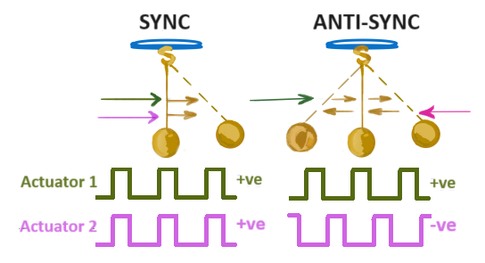
Figure 1: Each motor produces a pulse train. Left: the two pulse trains are in phase and have the same sign (SYNC). Right: the two pulse trains are in anti-phase and have opposite sign (ANTI-SYNC). Sketch courtesy of @artjoy2015.

In neuromorphic circuits, such rhythms are generated endogenously by simple neuronal motifs, inspired from the central pattern generators of neuroscience [22]. The simplest oscillating motif is the “half-centre oscillator” (HCO) [23]. An HCO comprises two ‘neurons’ connected by a pair of unidirectional interconnections called ‘synapses’. We arbitrarily label the neurons as neurons “A” and “B”. Each neuron is a circuit that produces bursts of voltage spikes. The synapses are inhibitory, meaning that they hinder spiking when active. The end of an inhibitory event causes the neuron to “rebound burst”. The mutual inhibitory coupling causes the neurons to produce bursts in anti-phase. Our neuromorphic architecture uses one artificial HCO per motor. The HCO drives the motor as follows: when neuron A is spiking, specifically when its voltage is above some threshold, the motor produces a constant torque. When the neuron is below this threshold, the motor is at rest. The mapping from neuron voltage to torque, and the switch in the sign of a torque, can be realised with an H-bridge and a DC motor. Fig. 2 shows the behavior of an HCO and its corresponding motor, for two burst sizes. A larger burst has more spikes, or spikes of longer duration.

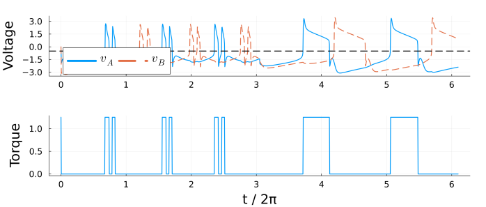
Figure 2: An HCO is made up of two neurons that burst in anti-phase. The size of the bursts can be modulated, as the simulation illustrates midway. Top: the voltages of the two neurons. The dashed horizontal line denotes the voltage threshold, above which the motor is active. Bottom: the torque of the corresponding motor.

The coordination between the two motors relies on synaptic interactions between the two HCOs. Excitatory synapses between the pair of A neurons, and also between the pair of B neurons, favors synchrony of the two HCOs. Inhibitory synapses between the same neurons favors anti-synchrony of the two HCOs. Fig. 3 shows the full network diagram. To switch motor configurations we switch the synaptic coupling, and also the sign of one of the motors. Fig. 4 shows one such network switch. The four-neuron circuit determines the automaton of the controller. Note the redundancy of this architecture as one neuron would in principle suffice to control the motor torque. This redundancy is typical of neuromorphic architectures. The two motor architecture could be easily generalised to an N-motor architecture, resulting in a highly distributed but also highly coordinated control architecture.

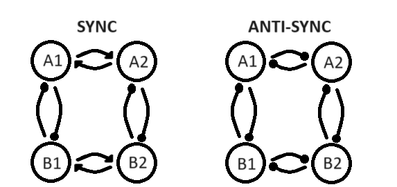
Figure 3: Diagram of the neuronal network. Neurons are denoted by circles, inhibitory synapses by ‘disc arrows’ and excitatory synapses by ‘pointed arrows’. The four synapses between the HCOs are either excitatory or inhibitory, for SYNC and ANTI-SYNC respectively.

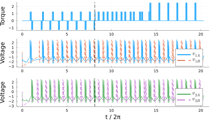
Figure 4: Simulation of the HCOs and actuators. Top: the total torque $I$. Middle: the voltages of HCO 1. Bottom: the voltages of HCO 2. At $t=8$ s (indicated by the dashed black line), the system’s configuration is switched from ANTI-SYNC and, after a transient period, it settles on SYNC.

IV Neuromorphic implementation

To enable the neuromodulation of the control circuit, we choose the neuron design in [24] which provides an easy relationship between the neuron parameters and the tuning of the bursting behavior. This neuron is an RC circuit and a bank of voltage-controlled current sources, all connected in parallel. Every current source provides either positive or negative conductance, at a particular timescale. A positive conductance is a source of negative feedback, and vice versa. The gains of the current sources are the control parameters. Each neuron $i$ has three state variables: a voltage $v_{i}$ (the output) and two low-pass-filtered voltages $v_{s,i}$ and $v_{us,i}$ (respectively ‘slow’ and ‘ultra-slow’ voltages). The dynamics are:

$$\tau_{f}\dot{v}_{i} =-v_{i}+{g_{f}^{-}}\tanh(v_{i})-{g_{s}^{+}}\tanh(v_{s,i})$$

$$+{g_{s}^{-}}\tanh(v_{s,i}+0.9)-{g_{us}^{+}}\tanh(v_{us,i}+0.9)$$

$$+I_{\rm{syn},ij}+{i_{\rm{app},i}}$$

$$\tau_{s}\dot{v}_{s,i} =v_{i}-v_{s,i}$$

$$\tau_{us}\dot{v}_{us,i} =v_{i}-v_{us,i}$$

for $i\in\{A1,B1,A2,B2\}$. The timescales are manually chosen to align the neurons’ behavior with the timescale of the pendulum.

The parameters ${g_{x}^{\pm}}>0$ are the gains; each one tunes the strength of one conductance acting in a given voltage range and a given timescale. For example, ${g_{f}^{-}}$ tunes the strength of the fast negative conductance. The neuron spikes because of the fast negative and slow positive conductances; this fast-slow mixed feedback motif is the essence of excitability and spiking. To obtain bursting rather than spiking, we require the slow negative and ultra-slow positive conductances to repeat the same mixed-feedback motif, but in a slower timescale and lower voltage range [11]. For simplicity, we tune all neurons with the same set of parameters. The behavior is, however, quite robust to parameter uncertainty.

The neuron’s input is the applied current ${i_{\rm{app},i}}$. We set ${i_{\rm{app},i}}$ to a nominal value ${i_{\rm{nominal}}}=-1$, although it must be decreased briefly in one neuron of each HCO in order to initiate the oscillations. A full list of the parameter values used in each figure is available with the attached code. All quantities in this letter are non-dimensional; see [24] for the circuit implementation.

For the synapses we also use the circuit proposed in [25]. The current for the synapse from neuron $j$ to neuron $i$ obeys

$$I_{\rm{syn},ij}=g_{\rm{syn},ij}/(1+\exp(-2(v_{s,j}+1)))$$

where $g_{\rm{syn},ij}$ is positive for an excitatory synapse, and negative for an inhibitory one.

V Control by entrainment

Section II suggests a simple control problem in the overdamped regime: we expect a monotone relationship between the energy injected into the system and the amplitude of oscillations. We choose a fixed frequency for the HCO controller that (roughly) matches the natural frequency of the pendulum, and we consider the anti-phase configuration that results in symmetric oscillations.

Fig. 5 shows entrainment at the fixed frequency for different choices of burst size. The amplitude increases with burst size, which is regulated by ${g_{s}^{-}}$. This gain also affects the frequency of the HCO, a variation compensated by the parameter ${g_{us}^{+}}$. Fig. 6 illustrates the monotonic relationship between the amplitude of the entrained pendulum and the neural gains ${g_{s}^{-}}$ and ${g_{us}^{+}}$, at the fixed frequency.

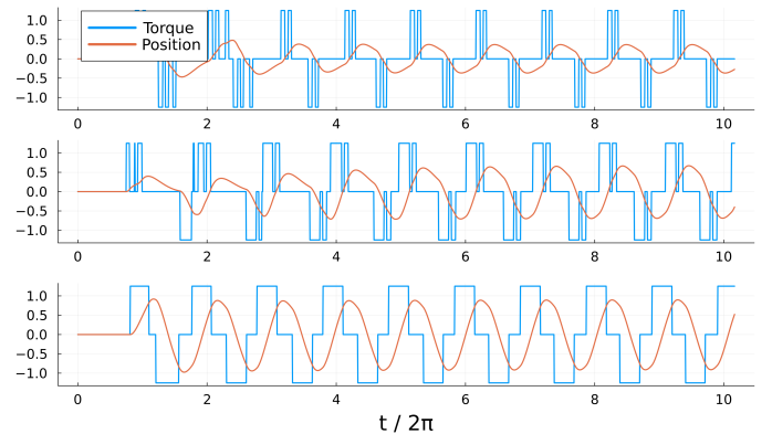
Figure 5: Small oscillations in the overdamped regime (damping $\alpha=1.4$). As the kick size of the neural oscillation increases (from top row to bottom row), so does the amplitude of the pendulum’s oscillation.

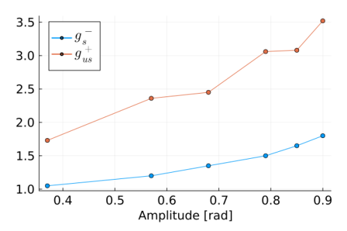
Figure 6: Entrainment of the pendulum at a fixed frequency in the overdamped regime ($\alpha=1.4$). The amplitude of small oscillations increases monotonically with ${g_{s}^{-}}$ and ${g_{us}^{+}}$.

For lower values of the damping, the behavior becomes more complex, following the prediction of Section II. Fig. 7 shows that, in the underdamped regime, small bursts in SYNC produce either small or large oscillations, depending on the initial conditions.

The left plot of Fig. 7 highlights that the sign of velocity does not vary in large oscillations, which therefore requires the SYNC configuration. The plot shows entrainment of large oscillations with two complete swings of the pendulum for every motor kick (a larger kick would produce more swings per period). However, and in contrast to the small-oscillation regime, the entrainment of large oscillations is fragile. A slight change to the parameters can lead to a non-periodic behaviour. Feedback control is necessary for the robust control of large oscillations (see Section VII).

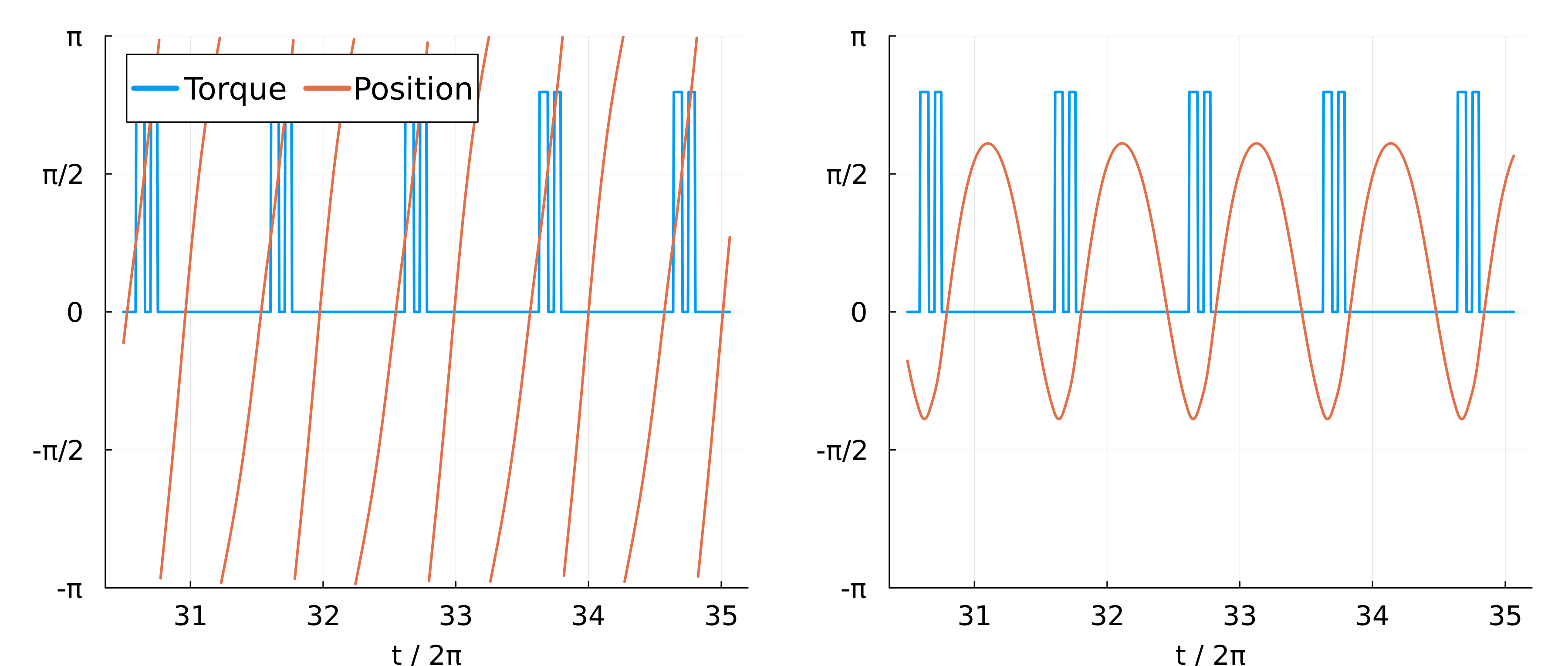
Figure 7: Entrainment with a SYNC neural oscillation in the underdamped regime (in this example, $\alpha=0.14$). Depending on the initial conditions, the steady-state oscillations are either large or small (shown by the left and right plots respectively). The large oscillations have 2 complete swings of the pendulum per period. Transients removed for clarity.

VI Neuromorphic Adaptive Control

The regulation of a desired frequency $\omega$ and amplitude $A$ can be achieved by combining the entrainment strategy described in the previous section with adaptive control of the two neural parameters ${g_{x}^{\pm}}$.

This builds on previous work [12, 13, 26, 27], where we demonstrated the robust adaptive control of neuron networks. The neuronal architecture inherently satisfies the standard assumptions of adaptive control: the system is minimum phase, relative degree one, and linear in the parameters. Adaptive control is analogous to the biological concept of neuromodulation [28].

We set a reference frequency ${\omega_{\rm{ref}}}$ and a reference amplitude ${A_{\rm{ref}}}$ for the pendulum’s oscillation. We also introduce the error signals $e_{\omega}=\omega-{\omega_{\rm{ref}}}$ and $e_{A}=A-{A_{\rm{ref}}}$. We adapt the two parameters ${g_{us}^{+}}$ and ${g_{s}^{-}}$ which regulate the neural frequency and burst size, respectively. The gains can only be varied within a limited range before the bursting behavior breaks down, which requires saturation of the adaptive gains. Instead of controlling ${g_{us}^{+}}$ and ${g_{s}^{-}}$ directly, we control saturated parameters ${\theta_{us}^{+}}$ and ${\theta_{s}^{-}}$. We set ${g_{us}^{+}}=\sigma_{\omega}({\theta_{us}^{+}})$ and ${g_{s}^{-}}=\sigma_{A}({\theta_{s}^{-}})$, where $\sigma_{\omega}(\cdot)$ and $\sigma_{A}(\cdot)$ are sigmoid functions with hand-designed minimum, maximum, offset and slope. These parameters are not totally decoupled (a change in ${g_{s}^{-}}$ also affects the frequency), but the feedback compensates for this. The basic control laws are ${\dot{\theta}_{us}^{+}}=-k_{\omega}e_{\omega}$ and ${\dot{\theta}_{s}^{-}}=-k_{A}e_{A}$, where $k_{\omega},k_{A}>0$ are constants. We also introduce dead-zones by setting ${\dot{\theta}_{us}^{+}}=0$ when $|e_{\omega}|<\delta_{\omega}$ and ${\dot{\theta}_{s}^{-}}=0$ when $|e_{A}|<\delta_{A}$, where $\delta_{\omega},\delta_{A}>0$ are constants.

This adaptive controller has been used to obtain the parameters of Fig. 6. The corresponding transient error correction is shown by Fig. 8. The adaptive controller also reduces the sensitivity of the amplitude to perturbations such as a change in mass.

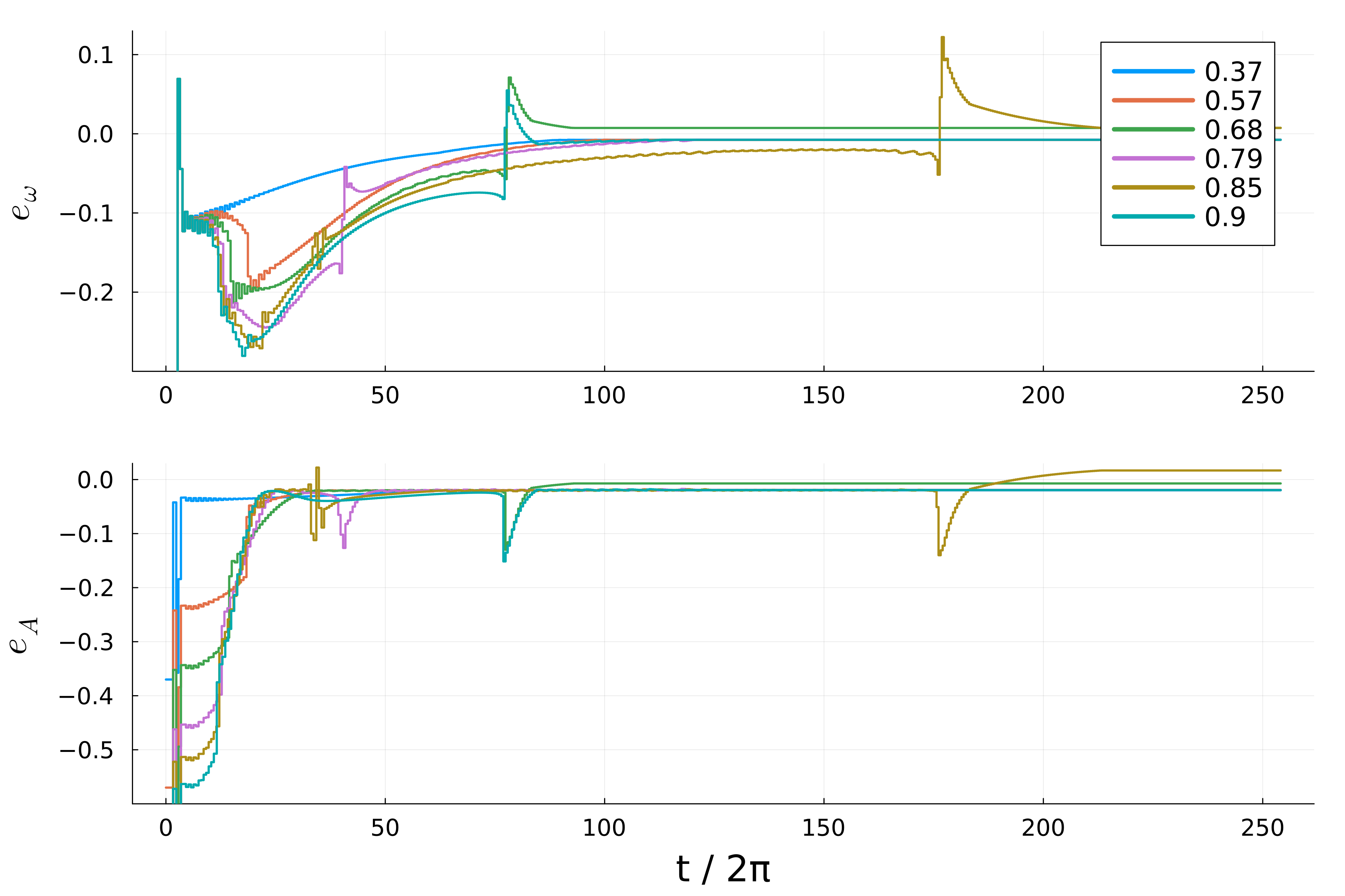
Figure 8: The error signals $e_{\omega}$ (top row) and $e_{A}$ (bottom row) of the adaptive controller, when used to obtain the parameters in Fig. 6. The legend gives the values of ${A_{\rm{ref}}}$ in radians. In each case, ${\omega_{\rm{ref}}}$ is the fixed frequency chosen in Section V.

VII Phase Control

In addition to neuromodulation, sensory information can also be used for phase control.

We use phase control to enlarge the basin of attraction of large oscillations in the underdamped regime. Bistability exists in that regime because there are two energy levels at which the energy ‘balances’, meaning that energy injected over a period is equal to energy dissipated. Depending on the initial conditions, the pendulum will converge to a low or high energy state (small or large oscillations respectively). The motors’ rate of energy injection is $\dot{E}=\dot{q}I$; the two states therefore have distinct phase differences between velocity and torque.

Phase control consists of small pulses that advance or delay the next rebound burst as illustrated in Fig. 9. The delay or advance resulting from an inhibitory pulse is a function of the timing of the pulse, a relationship known as the ‘phase response curve’ (PRC) [29]. A monotone phase response curve allows control of the phase of an oscillator by a simple proportional control [30]. The PRC method requires the perturbations to be small. We use perturbations of fixed amplitude (P) and fixed duration (w). Fig. 10 provides an empirical PRC of the HCO oscillator. The proportional feedback controller uses sensory events to determine the pulse timings: whenever there is an event of the form $q(t)=q_{\rm{phase}}$ (where $q_{\rm{phase}}$ is a controller parameter), the controller injects inhibitory pulses into two of the four neurons. The choice of the two neurons is such that the controller in steady-state respects the fixed phase relationships between neurons. The control signal into neuron $i$ is ${i_{\rm{pulse},i}}$ and the total input is ${i_{\rm{app},i}}={i_{\rm{nominal}}}+{i_{\rm{pulse},i}}$.

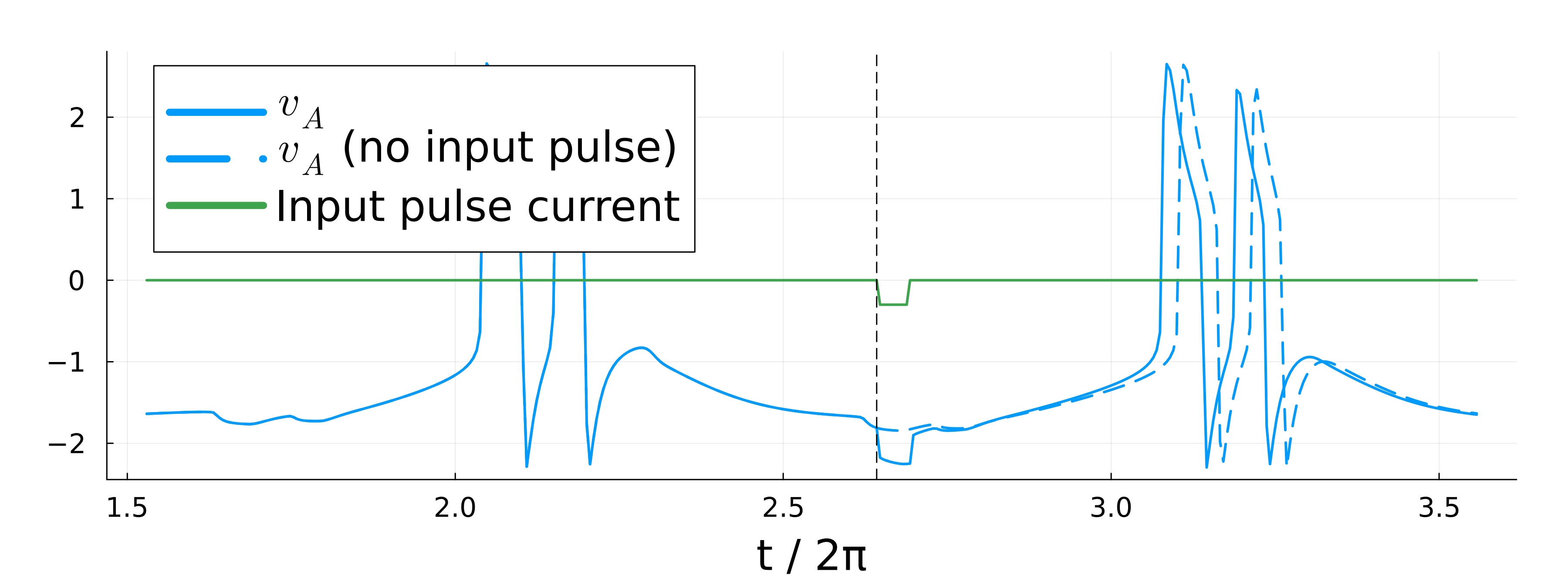
Figure 9: A small inhibitory pulse causes a phase advance or delay of the next rebound burst. The simulation is for an isolated HCO (only $v_{A}$ is shown). The blue dashed curve shows the behaviour of $v_{A}$ in the absence of the pulse.

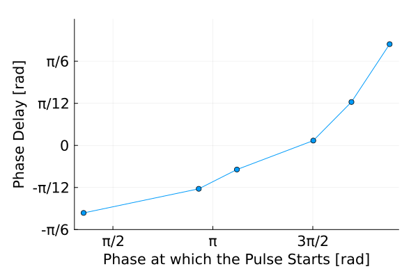
Figure 10: Phase response curve of an HCO. The curve indicates the phase shift resulting from a fixed pulse ($w=0.05$ s and $P=0.3$) as a function of the timing of the pulse along the limit cycle.

Fig. 11 illustrates the stabilizing property of a proportional phase control on the behavior illustrated in fig. 7 (right plot). The phase control stabilizes the large oscillations to a constant period. We selected $q_{\rm{phase}}=-1$ rad such that small oscillations are prevented. To prevent braking during the transient, a sensory event is ignored if the pendulum’s velocity is negative.

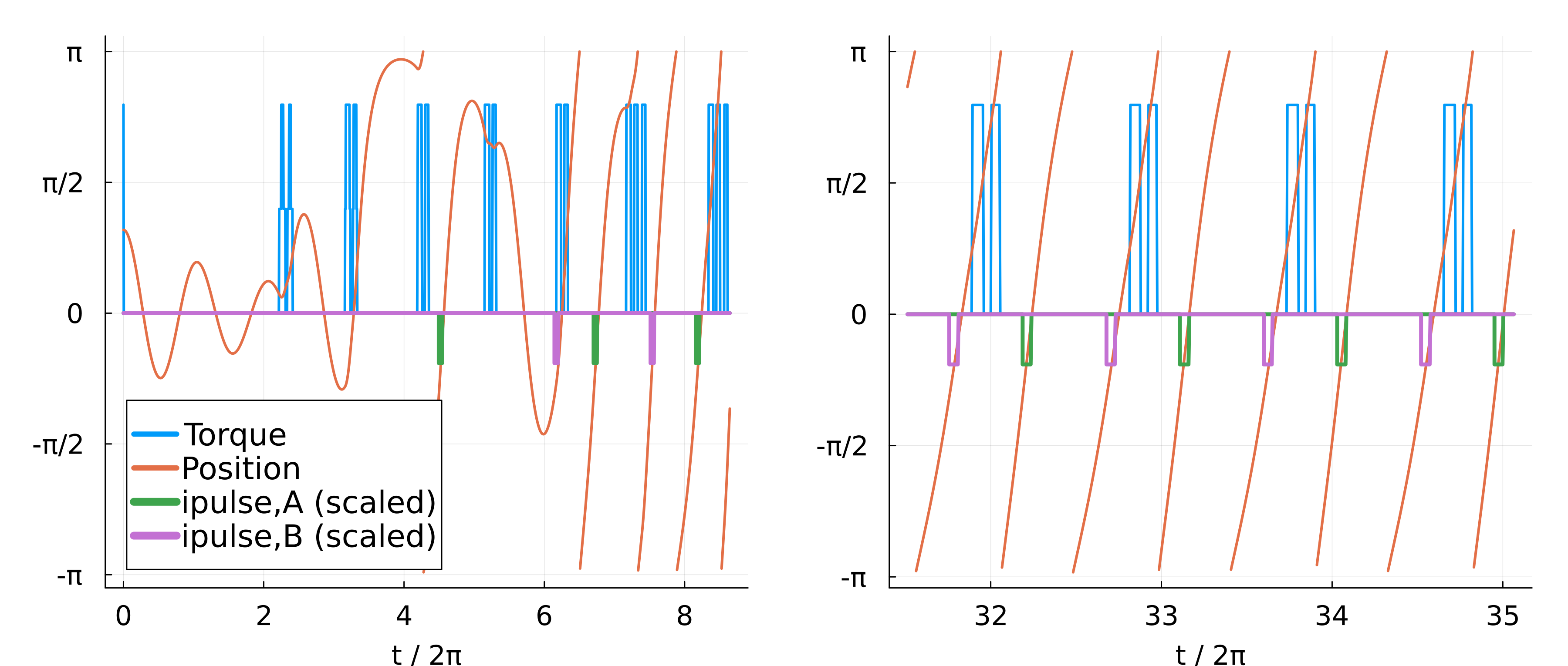
Figure 11: The simulation of fig. 7 (right plot) with the addition of phase control. Large oscillations are now entrained. There is a slight change in frequency due to a constant steady-state error in phase. The current pulses to the A and B neurons are shown in green and purple respectively, and are scaled for clarity. The two plots are from the same simulation; they show both the initial part of the transient and the steady-state behaviour.

VIII Conclusion

We have presented a neuromorphic, event-based framework for controlling the oscillations of a mechanical pendulum. A simple neuronal network is used to generate rhythmic events capable of entraining the rhythmic behaviors of the pendulum. Adaptive control regulates the entrainment. Phase control enlarges the basin of attraction of a desired oscillation.

The event-based control strategy is inherently robust to model and controller uncertainties because of the high impedance but highly localised-in-time nature of the interactions.

The approach of this letter is general, and applies to a wide range of mechanical systems. Indeed, one need not stray too far from the pendulum itself to find familiar robotic or biomechanical rhythms: the ’inverted pendulum’ model lies at the foundation of the literature on walking [31, 32]. It consists of two rigid legs, one a pendulum, the other an inverted pendulum. To include a second state, running, add springs [33]. Meanwhile, multiple HCOs can be chained together to drive an amphibious lamprey-like robot that walks and swims [4]. Compliance is another topic of interest; owing to the high localised but low average impedance, pulse-based actuation suggests a path to overcoming the stiffness-compliance trade-off [34]. We hope that this letter will motivate such investigations in more challenging robotic designs.

References

- [1] D. Lakatos, F. Petit, and A. Albu-Schäffer, “Nonlinear oscillations for cyclic movements in human and robotic arms,” IEEE Transactions on Robotics, vol. 30, no. 4, pp. 865–879, 2014.
- [2] M. M. Williamson, “Robot arm control exploiting natural dynamics,” Ph.D. dissertation, Massachusetts Institute of Technology, 1999.
- [3] G. Garofalo, C. Ott, and A. Albu-Schäffer, “Walking control of fully actuated robots based on the bipedal slip model,” in 2012 IEEE International Conference on Robotics and Automation. IEEE, 2012, pp. 1456–1463.
- [4] A. J. Ijspeert, A. Crespi, D. Ryczko, and J.-M. Cabelguen, “From swimming to walking with a salamander robot driven by a spinal cord model,” science, vol. 315, no. 5817, pp. 1416–1420, 2007.
- [5] C. Mead, Analog VLSI and neural systems. Addison-Wesley Longman Publishing Co., Inc., 1989.
- [6] S. P. DeWeerth, L. Nielsen, C. A. Mead, and K. J. Åström, “A simple neuron servo,” IEEE Transactions on Neural Networks, vol. 2, no. 2, pp. 248–251, 1991.
- [7] K.-E. Åarzén, “A simple event-based pid controller,” IFAC Proceedings Volumes, vol. 32, no. 2, pp. 8687–8692, 1999.
- [8] E. Aranda-Escolastico, M. Guinaldo, R. Heradio, J. Chacon, H. Vargas, J. Sánchez, and S. Dormido, “Event-based control: A bibliometric analysis of twenty years of research,” IEEE Access, vol. 8, pp. 47 188–47 208, 2020.
- [9] R. Sepulchre, “Spiking control systems,” Proceedings of the IEEE, 2022.
- [10] C. Fernandez Lorden, “Neuromorphic control of embodied central pattern generators,” Université de Liège, Liège, Belgique, 2023, (Unpublished master’s thesis), https://matheo.uliege.be/handle/2268.2/18256.
- [11] L. Ribar and R. Sepulchre, “Neuromorphic control: Designing multiscale mixed-feedback systems,” IEEE Control Systems Magazine, vol. 41, no. 6, pp. 34–63, 2021.
- [12] R. Schmetterling, T. B. Burghi, and R. Sepulchre, “Adaptive conductance control,” Annual Reviews in Control, 2022.
- [13] T. B. Burghi and R. Sepulchre, “Adaptive observers for biophysical neuronal circuits,” IEEE Transactions on Automatic Control, 2023.
- [14] A. J. Ijspeert, “Central pattern generators for locomotion control in animals and robots: a review,” Neural networks, vol. 21, no. 4, pp. 642–653, 2008.
- [15] A. J. Ijspeert, A. Crespi, and J.-M. Cabelguen, “Simulation and robotics studies of salamander locomotion: applying neurobiological principles to the control of locomotion in robots,” Neuroinformatics, vol. 3, pp. 171–195, 2005.
- [16] E. Angelidis, E. Buchholz, J. Arreguit, A. Rougé, T. Stewart, A. von Arnim, A. Knoll, and A. Ijspeert, “A spiking central pattern generator for the control of a simulated lamprey robot running on spinnaker and loihi neuromorphic boards,” Neuromorphic Computing and Engineering, vol. 1, no. 1, p. 014005, 2021.
- [17] H. X. Ryu and A. D. Kuo, “An optimality principle for locomotor central pattern generators,” Scientific Reports, vol. 11, no. 1, p. 13140, 2021.
- [18] M. A. Lewis, F. Tenore, and R. Etienne-Cummings, “Cpg design using inhibitory networks,” in Proceedings of the 2005 IEEE international conference on robotics and automation. IEEE, 2005, pp. 3682–3687.
- [19] M. F. Simoni and S. P. DeWeerth, “Two-dimensional variation of bursting properties in a silicon-neuron half-center oscillator,” IEEE Transactions on Neural Systems and Rehabilitation Engineering, vol. 14, no. 3, pp. 281–289, 2006.
- [20] A. D. Kuo, “The relative roles of feedforward and feedback in the control of rhythmic movements,” Motor control, vol. 6, no. 2, pp. 129–145, 2002.
- [21] S. H. Strogatz, “Nonlinear dynamics and chaos,” 1996.
- [22] D. Bucher, G. Haspel, J. Golowasch, and F. Nadim, “Central pattern generators,” eLS, pp. 1–12, 2015.
- [23] E. Marder, S. Kedia, and E. O. Morozova, “New insights from small rhythmic circuits,” Current opinion in neurobiology, vol. 76, p. 102610, 2022.
- [24] L. Ribar and R. Sepulchre, “Neuromodulation of neuromorphic circuits,” IEEE Transactions on Circuits and Systems I: Regular Papers, vol. 66, no. 8, pp. 3028–3040, 2019.
- [25] L. Ribar, “Synthesis of neuromorphic circuits with neuromodulatory properties,” Ph.D. dissertation, University of Cambridge, 2020.
- [26] R. Schmetterling, T. B. Burghi, and R. Sepulchre, “Robust online estimation of biophysical neural circuits,” in 2023 62nd IEEE Conference on Decision and Control (CDC). IEEE, 2023, pp. 703–708.
- [27] T. B. Burghi, T. O’Leary, and R. Sepulchre, “Distributed online estimation of biophysical neural networks,” in 2022 IEEE 61st Conference on Decision and Control (CDC). IEEE, 2022, pp. 628–634.
- [28] E. Marder, T. O’Leary, and S. Shruti, “Neuromodulation of circuits with variable parameters: single neurons and small circuits reveal principles of state-dependent and robust neuromodulation,” Annual review of neuroscience, vol. 37, pp. 329–346, 2014.
- [29] P. Sacre and R. Sepulchre, “Sensitivity analysis of oscillator models in the space of phase-response curves: Oscillators as open systems,” IEEE Control Systems Magazine, vol. 34, no. 2, pp. 50–74, 2014.
- [30] D. Efimov, P. Sacré, and R. Sepulchre, “Controlling the phase of an oscillator: a phase response curve approach,” in Proceedings of the 48h IEEE Conference on Decision and Control (CDC) held jointly with 2009 28th Chinese Control Conference. IEEE, 2009, pp. 7692–7697.
- [31] M. Garcia, A. Chatterjee, A. Ruina, and M. Coleman, “The simplest walking model: stability, complexity, and scaling,” 1998.
- [32] A. D. Kuo, “A simple model of bipedal walking predicts the preferred speed–step length relationship,” J. Biomech. Eng., vol. 123, no. 3, pp. 264–269, 2001.
- [33] H. Geyer, A. Seyfarth, and R. Blickhan, “Compliant leg behaviour explains basic dynamics of walking and running,” Proceedings of the Royal Society B: Biological Sciences, vol. 273, no. 1603, pp. 2861–2867, 2006.
- [34] G. A. Pratt, M. M. Williamson, P. Dillworth, J. Pratt, and A. Wright, “Stiffness isn’t everything,” in Experimental Robotics IV: The 4th International Symposium, Stanford, California, June 30–July 2, 1995. Springer, 1997, pp. 253–262.