Jammer-Resilient Time Synchronization
in the MIMO Uplink

Abstract

Spatial filtering based on multiple-input multiple-output (MIMO) processing is a promising approach to jammer mitigation. Effective MIMO data detectors that mitigate smart jammers have recently been proposed, but they all assume perfect time synchronization between transmitter(s) and receiver. However, to the best of our knowledge, there are no methods for resilient time synchronization in the presence of smart jammers. To remedy this situation, we propose JASS, the first method that enables reliable time synchronization for the single-user MIMO uplink while mitigating smart jamming attacks. JASS detects a randomized synchronization sequence based on a novel optimization problem that fits a spatial filter to the time-windowed receive signal in order to mitigate the jammer. We underscore the efficacy of the proposed optimization problem by proving that it ensures successful time synchronization under certain intuitive conditions. We then derive an efficient algorithm for approximately solving our optimization problem. Finally, we use simulations to demonstrate the effectiveness of JASS against a wide range of different jammer types.

I Introduction

Jammers must be mitigated as they pose a serious threat to the wireless communication infrastructure [1, 2, 3]. Multiple-input multiple-output (MIMO) processing methods enable spatial filtering and have therefore been recognized as a promising approach for jammer mitigation [4, 5, 6, 7, 8, 9, 10, 11, 12, 13, 14, 15]. If the MIMO receiver has more antennas than the jammer (a typical assumption in the context of MIMO jammer mitigation), then the jammer interference can only occupy a lower-dimensional subspace of the entire signal space, which enables nulling by projecting the receive signals on the orthogonal complement of that subspace [6, 7, 8, 11, 12, 9, 10, 13] or by attenuating the signal dimensions that correspond to the jammer’s subspace during equalization [11, 12, 13, 15, 14]. These basic mechanisms are surrounded, however, by a myriad of issues, such as how the relevant quantities of the jammer’s spatial signature (i.e., its subspace or its spatial covariance matrix) can be estimated at the receiver [5, 6, 7, 8, 11, 9, 10, 12, 13, 14] or how a link between the receiver and a legitimate transmitter can be established [7, 14, 8, 16, 17, 18, 19, 20, 21, 22]. These latter questions are exacerbated when a strong attack model is considered in which the jammer is not assumed to behave in some predictable manner (such as steadily transmitting at all times, or when the legitimate transmitter is transmitting) that can be exploited for mitigation. Recently, there has been considerable progress on how to estimate the spatial signature of smart jammers [6, 9, 10, 13], but all of these methods assume that a communication link between the receiver and the legitimate transmitter(s) has already been established, i.e., it is typically assumed that (i) the receiver knows of the existence of the legitimate transmitter(s) and (ii) the receiver and transmitter(s) are synchronized in time and frequency. These assumptions are far from innocent since smart jammers can attack also the procedures for link establishment [18, 19, 20]. Several methods have been proposed for synchronization in the presence of jamming [23, 21, 22, 7, 14, 8], but none of them assume a strong attack model in the sense of [9, 10, 13].

I-A Contributions

We propose JASS (short for Jammer-Aware SynchroniSation), the first method that enables reliable time synchronization against arbitrary jamming attacks, including attacks from smart multi-antenna jammers. JASS relies on MIMO processing to mitigate jammers via adaptive spatial filtering. Specifically, we propose a novel optimization problem for detecting the presence (or absence) of a randomized synchronization sequence (that is known to both the transmitter and the receiver, but not to the jammer) at time $\ell$ by fitting a spatial filter to the time-windowed receive signal—if the optimized objective value exceeds a certain threshold, then the receiver decides that the synchronization sequence has been transmitted at the corresponding time instant $\ell$. We prove that, under certain intuitive conditions, solving this optimization problem will detect the synchronization sequence correctly with probability one. Since the optimization problem in question is nonconvex, the JASS synchronization algorithm utilizes an efficient procedure (closely related to Dinkelbach’s method [24]) for approximately solving our optimization problem. We demonstrate the effectiveness of JASS using simulations that consider a broad range of jammer types. In particular, JASS is, to the best of our knowledge, the only time synchronization method that can mitigate all of the considered jammer types without requiring or exploiting any explicit information about the jammer’s type or behavior.

I-B Related Work

The impact of jamming attacks on synchronization has been discussed in [16] and in [18, 17]. The latter two works also mention the danger of preamble spoofing to synchronization. Different protocol specific attacks against LTE and 5G NR, including jamming and spoofing of synchronization signals, are discussed in [19, 20]. As countermeasures against spoofing attacks, reference [17] advocates for randomized preambles. Similarly, references [23, 21] propose to randomize the in-frame position of synchronization signals, but this countermeasure is effective only against jammers that try to be stealthy by only jamming synchronization signals, but not against barrage jammers that jam continuously. In [22], an adaptive filter with frequency-dependent weights is proposed as a method for LTE synchronization that is resilient against partial-band jammers, but this approach remains vulnerable to full-spectrum barrage jamming. In contrast to these works, our approach mitigates jammers through spatial filtering and does not depend on any particular jamming strategy (such as jamming only synchronization signals or partial-band jamming). Moreover, since our approach builds upon on a randomized synchronization sequence, it is invulnerable to spoofing.

The papers [7, 14, 8] implement MIMO jammer mitigation on Universal Software Radio Peripherals (USRPs) and their implementations include methods for time synchronization. The work in [7] detects the start of a transmitted frame based on the following insight: If the received signal contains both UE and jamming signals, then the receive vectors $\mathbf{y}[k]$ and $\mathbf{y}[k^{\prime}]$ will in general not be collinear for $k^{\prime}\neq k$, while, if the receive signal only contains jamming signals from a single-antenna jammer but no UE signals, then $\mathbf{y}[k]$ and $\mathbf{y}[k^{\prime}]$ will be collinear. However, if the jammer is much stronger than the UE, a large number of receive samples is needed to decide between these two hypotheses (500 samples are used in [7]). Moreover, this insight can only be used to mitigate single-antenna jammers, since multi-antenna jammers can generate receive vectors that are not necessarily collinear across different samples. The work in [14] uses a spatial filter to null the jammer interference during the synchronization phase. For this, however, one must assume a barrage jammer which jams permanently, so that its spatial signature can be estimated from the receive signals during a training phase. The work in [8] considers a reactive jammer that only starts to jam after the frame start. This work depends on the assumption that the jammer’s reaction time is sufficiently slow so that the transmit signal preamble (which includes synchronization signals) is not jammed. In contrast to these works, our method mitigates jammers regardless of whether they have one or multiple antennas, and regardless of whether they jam permanently or only at selected instants.

In summary, we find no synchronization method designed to withstand strong jamming attacks in the sense of [9, 10, 13], where the jammer is not assumed to behave in some predictable way that can be exploited for mitigation. Moreover, none of these works on mitigation consider jammers which behave in ways that should make it difficult for the receiver to mitigate it (such as transmitting in erratic bursts, switching between different transmit antennas to dynamically change its spatial signature, or transmitting only at instances when the legitimate transmitter is transmitting). Our paper fills this gap by (i) assuming a strong attack model in the first place and (ii) by specifically considering such adversarial jammers in the empirical evaluation of our method.

I-C Notation

Matrices and column vectors are written in boldface uppercase and lowercase letters, respectively. For a matrix $\mathbf{A}\in\mathbb{C}^{M\times N}$ (and analogously for a vector $\mathbf{a}\in\mathbb{C}^{M}$), the conjugate is $\mathbf{A}^{\ast}$, the transpose is $\mathbf{A}^{T}$, the conjugate transpose is $\mathbf{A}^{H}$, and the pseudo-inverse is $\mathbf{A}^{\dagger}$. The Frobenius norm is $\|\cdot\|_{F}$, and $\|\cdot\|_{2}$ denotes the spectral norm (for matrices) and the Euclidean norm (for vectors), respectively. The columnspace and rowspace of $\mathbf{A}$ are $\textit{col}(\mathbf{A})$ and $\textit{row}(\mathbf{A})$, respectively. Horizontal concatenation of two matrices $\mathbf{A}$ and $\mathbf{B}$ is denoted by $[\mathbf{A},\mathbf{B}]$; vertical concatenation is $[\mathbf{A};\mathbf{B}]$. The $N\times N$ identity matrix is $\mathbf{I}_{N}$, $\mathbf{1}_{N}=[1;\dots;1]\in\mathbb{C}^{N}$ is the $N\times 1$ all-ones vector, and $[N:N^{\prime}]$ denotes the integers from $N$ through $N^{\prime}\geq N$. The all-zero vector (whose dimension is implicit) is $\mathbf{0}$. The distribution of a circularly-symmetric complex Gaussian vector with covariance matrix $\mathbf{C}$ is denoted by $\mathcal{C}\mathcal{N}(\mathbf{0},\mathbf{C})$.

II System Model

II-A System Model and Problem Formulation

We consider the uplink of a multi-antenna system in which a single-antenna UE wants to synchronize to a $B$-antenna BS in presence of an $I$-antenna jammer (or multiple jammers with $I$ antennas in total) with $I<B$. To this end, the UE transmits a length-$K$ synchronization sequence $\check{}\mathbf{s}=[\check{s}_{0},\dots,\check{s}_{K-1}]^{T}\!\in\!\mathbb{C}^{K}$ that is known to the BS, but assumed to be unknown to the jammer. We model the time synchronization problem from the vantage point of the BS, which has to detect the instant at which the UE transmits the synchronization sequence. We assume flat fading and describe the receive signal at the BS at sample index $k\in\mathbb{Z}_{\geq 0}$ as

$$\mathbf{y}[k]=\mathbf{h}s[k-L]+\mathbf{J}\mathbf{w}[k]+\mathbf{n}[k].$$ (1)

Here, $\mathbf{y}[k]\in\mathbb{C}^{B}$ is the BS receive vector at sample index $k$; $s[\cdot]$ is the UE transmit signal, which we model as

$$s[k]=\begin{cases}0&:~{}~{}k<0\\ \check{s}_{k}&:~{}~{}k\in\{0,1,\dots,K-1\}\\ \text{undefined}&:~{}~{}k\geq K;\end{cases}$$ (2)

$L\in\mathbb{Z}_{\geq 0}$ represents the time at which the UE transmits the synchronization sequence—this is unknown a priori to the BS; $\mathbf{h}\in\mathbb{C}^{B}$ and $\mathbf{J}\in\mathbb{C}^{B\times I}$ model the channels from the UE to the BS and from the jammer to the BS, respectively, where the $i$th column of $\mathbf{J}$ holds the channel vector from the jammer’s $i$th antenna to the BS; $\mathbf{w}[k]\in\mathbb{C}^{I}$ is the jammer’s transmit signal at sample index $k$; and $\mathbf{n}[k]\sim\mathcal{C}\mathcal{N}(\mathbf{0},N_{0}\mathbf{I}_{B})$ is additive white circularly-symmetric complex Gaussian noise with per-entry variance $N_{0}$. Neither $\mathbf{h}$ nor $\mathbf{J}$ are known at the BS. And, apart from flat fading, we assume no particular channel model.

The time synchronization problem to be solved is the following: Based on a sequence of receive vectors $\{\mathbf{y}[k]\}_{k\geq 0}$, the BS has to produce an estimate $\hat{\ell}$ of the time index $L$, which we model as a non-negative integer-valued random variable. We consider it a synchronization failure if the BS fails to produce the correct estimate $\hat{\ell}=L$ immediately after having received $\{\mathbf{y}[k]\}_{0\leq k<K+L}$ and a success otherwise.

II-B Assumptions and Limitations

We now discuss several assumptions on which our model builds and the limitations that follow from these assumptions. In particular, we discuss (i) the fact that the synchronization sequence is sent by the UE and not the BS, (ii) the assumptions made on the synchronization sequence $\check{}\mathbf{s}$, and (iii) the assumptions made on the jammer’s transmit signal $\mathbf{w}[\cdot]$.

II-B1 Uplink synchronization

In currently deployed cellular systems such as 5G NR, it is the BS (and not the UE) that transmits synchronization signals [25], so that UEs adapt to the BS’s schedule. If the UE sends the synchronization signal (as in our model), then the BS has to adapt to the UE’s schedule, which makes it impossible to coordinate multiple UEs with each other. As a result, serving multiple UEs simultaneously becomes much more challenging. However, mitigating jammers in the downlink is an even more formidable problem than in the uplink, since the UEs typically have only one or few antennas and thus, cannot use spatial filtering for effective jammer mitigation [26]. In this paper, we limit our focus to establishing a robust uplink connection and leave the problem of establishing a robust downlink connection for future work. We note, however, that our setup can straightforwardly be adapted for point-to-point MIMO systems in which jammers can be mitigated at both multi-antenna receivers.

II-B2 Randomized synchronization sequence

We assume that the synchronization sequence $\check{}\mathbf{s}$ is known only to the UE and the BS, but not to the jammer. To this end, we draw a random sequence $\check{}\mathbf{s}\sim\mathcal{C}\mathcal{N}(\mathbf{0},\mathbf{I}_{K})$ with unit symbol energy in expectation: $\operatorname{\mathbb{E}}\mathopen{}\left[\|\check{}\mathbf{s}\|_{2}^{2}\right]=K$. In a practical implementations, both the UE and the BS could construct $\check{}\mathbf{s}$ using a Gaussian-like pseudo-random function that they seed with a pre-shared secret. The assumption that the jammer does not know $\check{}\mathbf{s}$ is paramount. Otherwise, the jammer could simply transmit a copy of $\check{}\mathbf{s}$—before the UE does—to fool the BS into erroneously detecting the synchronization sequence. To prevent the jammer from learning the synchronization sequence over time, the synchronization sequence should be different after every use. Which synchronization sequence is currently valid could, e.g., be tied to absolute time (provided that the UE and the BS have sufficiently accurate local estimates of absolute time).

II-B3 Strong attack model

Keeping step with our earlier work [9, 10, 13], to enable the mitigation of as manny different jammers as possible (and, in particular, of smart jammers), we want to develop a method that relies on as few assumptions about the jammer’s transmit behavior as possible. For this reason, we assume neither independence between the processes $\{\mathbf{w}[k]\}$ and $\{s[k]\}$, nor any particular distribution for $\{\mathbf{w}[k]\}$. In particular, we do not assume that the jammer behaves in time-invariant manner. We only make the following assumption about the jammer’s behavior: Since the jammer does not know $\check{}\mathbf{s}$, it follows that its transmit signal cannot depend non-causally on $\check{}\mathbf{s}$. More precisely, it follows that $\mathbf{w}[k+L]$ cannot depend on $\check{s}_{k+1},\dots,\check{s}_{K-1}$. To work with the strongest possible attack model, we therefore assume only that the jammer’s transmit signal $\mathbf{w}[k]$ at time $k$ cannot depend on $s[k^{\prime}]$ for $k^{\prime}>k$, but $\mathbf{w}[k]$ can depend on $s[k^{\prime}]$ for all $k^{\prime}\leq k$ (including $k^{\prime}=k$). In particular, we assume that the jammer can instantaneously recover the UE’s transmit signal and transmit any function thereof such as, e.g., the synchronization sequence itself. However, the jammer cannot transmit the synchronization seqeuence earlier than the UE. Moreover, we do not assume the strength of the jammer interference to be known at the BS. And, we also take into account that the number of jammer antennas $I$ may not be known at the BS.

II-B4 Other limitations

Our method is currently limited to frequency-flat communication channels. An extension to frequency-selective channels (i.e., channels with inter-symbol interference) is left for future work. Also, our method currently only enables time synchronization but not frequency synchronization (e.g., estimating and compensating carrier frequency and sampling rate offsets). This extension is also left for future work.

III Jammer-Resilient Time Synchronization

III-A The Optimization Problem

We now derive our approach for solving the time synchronization problem outlined in sec:problem. We start by considering time synchronization for communication systems that do not suffer from jamming. In that case, a sensible method is correlating the receive signal with the synchronization sequence, and declaring the synchronization sequence to be detected when the correlation exceeds a certain threshold $\tau$. Mathematically, this goal can be expressed as solving

$$\operatorname*{arg\;min}_{\ell\in\mathbb{Z}_{\geq 0}}\ell\quad\text{s.t.}\quad\left\|\sum_{k=0}^{K-1}\mathbf{y}[k+\ell]\check{s}_{k}^{\ast}\right\|_{2}^{2}\geq\tau.$$ (3)

In the presence of jamming, however, the constraint objective $\big{\|}\sum_{k=0}^{K-1}\mathbf{y}[k+\ell]\check{s}_{k}^{\ast}\big{\|}_{2}^{2}$ will be affected heavily by the jammer interference. In particular, the constraint objective increases (with high probability) as the interference power increases. In the presence of jamming, solving (3) is therefore not reliable for time synchronization.

A naïve strategy to compensate for the constraint objective’s dependence on the interference power would be to normalize the constraint objective with the (windowed) receive energy:

$$\operatorname*{arg\;min}_{\ell\in\mathbb{Z}_{\geq 0}}\ell\quad\text{s.t.}\quad\frac{\left\|\sum_{k=0}^{K-1}\mathbf{y}[k+\ell]\check{s}_{k}^{\ast}\right\|_{2}^{2}}{\sum_{k=0}^{K-1}\left\|\mathbf{y}[k+\ell]\right\|_{2}^{2}}\geq\tau.$$ (4)

However, our simulations in sec:eval will show that this approach, too, fares poorly in the presence of strong jamming.

In order to achieve jammer-resilient time synchronization, we therefore leverage spatial filtering: If the jammer channel matrix $\mathbf{J}$ were known at the BS, then the BS could project the receive signal $\mathbf{y}[k]$ onto the orthogonal complement of $\textit{col}(\mathbf{J})$ by multiplying it with the projection matrix $\mathbf{P}=\mathbf{I}_{B}-\mathbf{J}\mathbf{J}^{\dagger}$ to obtain the jammer-free input-output relation

$$\mathbf{P}\mathbf{y}[k] =\mathbf{P}\mathbf{h}s[k-L]+\underbrace{\mathbf{P}\mathbf{J}}_{=\,\mathbf{0}}\mathbf{w}[k]+\mathbf{P}\mathbf{n}[k]$$ (5)

$$=\mathbf{P}\mathbf{h}s[k-L]+\mathbf{P}\mathbf{n}[k].$$ (6)

The synchronization sequence could then easily be detected using a correlation-based approach analogous to (3) or (4). In practice, however, $\mathbf{J}$ is not known at the BS—at least not a priori. Moreover, we cannot take for granted that the jammer is active during any specific period of time. Thus, we cannot estimate $\mathbf{J}$ from any fixed set of receive vectors; see also the related discussions in [9, 10, 13].

In order to spatially mitigate the jammer despite not knowing its channel, our approach will be as follows: Let $\hat{I}$ be the BS’s guess of how many antennas the jammer has at most. For any possible time index $\ell$ at which the synchronization sequence could have been transmitted, we fit a projection of the form $\tilde{}\mathbf{P}=\mathbf{I}_{B}-\mathbf{A}\mathbf{A}^{H},\mathbf{A}\in\mathcal{O}^{B\times\hat{I}}$ (where $\mathcal{O}^{B\times\hat{I}}$ is the set of $B\times\hat{I}$ sized matrices with orthonormal columns, the elements of which satisfy $\mathbf{A}^{\dagger}=\mathbf{A}^{H}$) to the windowed receive signal $\mathbf{y}[\ell],\dots,\mathbf{y}[\ell+K-1]$. The set of all such projections $\tilde{}\mathbf{P}$ is the Grassmannian manifold

$$\mathscr{G}_{B-\hat{I}}(\mathbb{C}^{B})=\left\{\mathbf{I}_{B}-\mathbf{A}\mathbf{A}^{H}:\mathbf{A}\in\mathcal{O}^{B\times\hat{I}}\right\}\!,$$ (7)

and the $\tilde{}\mathbf{P}\in\mathscr{G}_{B-\hat{I}}(\mathbb{C}^{B})$ with the best fit is the one for which the projected receive sequence $\tilde{}\mathbf{P}\mathbf{y}[k]$ exhibits the highest normalized correlation with the synchronization sequence $\check{}\mathbf{s}$. Mathematically, this fitting of the projection $\tilde{}\mathbf{P}$ to the receive signal windowed at time index $\ell$ can be expressed through the following optimization problem:

$$\max_{\tilde{}\mathbf{P}\in\mathscr{G}_{B-\hat{I}}(\mathbb{C}^{B})}\frac{\left\|\tilde{}\mathbf{P}\sum_{k=0}^{K-1}\mathbf{y}[k+\ell]\check{s}_{k}^{\ast}\right\|_{2}^{2}}{\sum_{k=0}^{K-1}\left\|\tilde{}\mathbf{P}\mathbf{y}[k+\ell]\right\|_{2}^{2}}.$$ (8)

By defining the windowed receive matrix

$$\mathbf{Y}_{\ell}=[\mathbf{y}[\ell],\mathbf{y}[\ell+1],\dots,\mathbf{y}[\ell+K-1]]\in\mathbb{C}^{B\times K},$$ (9)

we can rewrite (8) as

$$\max_{\tilde{}\mathbf{P}\in\mathscr{G}_{B-\hat{I}}(\mathbb{C}^{B})}\frac{\|\tilde{}\mathbf{P}\mathbf{Y}_{\ell}\check{}\mathbf{s}^{\ast}\|_{2}^{2}}{\|\tilde{}\mathbf{P}\mathbf{Y}_{\ell}\|_{F}^{2}}.$$ (10)

Concerning the objective of (10), we define $\frac{\|\tilde{}\mathbf{P}\mathbf{Y}_{\ell}\check{}\mathbf{s}^{\ast}\|_{2}^{2}}{\|\tilde{}\mathbf{P}\mathbf{Y}_{\ell}\|_{F}^{2}}\triangleq 0$ if $\|\tilde{}\mathbf{P}\mathbf{Y}_{\ell}\check{}\mathbf{s}^{\ast}\|_{2}^{2}=0$ and $\|\tilde{}\mathbf{P}\mathbf{Y}_{\ell}\|_{F}^{2}=0$. We propose to estimate the time index $L$ in (1) by the lowest index $\ell$ for which the solution of the optimization problem in (8) exceeds some threshold $\tau$: $\displaystyle\operatorname*{arg\;min}_{\ell\in\mathbb{Z}_{\geq 0}}~{}\ell\!\quad\textnormal{s.t.}\quad\!\!\max_{\tilde{}\mathbf{P}\in\mathscr{G}_{B-\hat{I}}(\mathbb{C}^{B})}\frac{\|\tilde{}\mathbf{P}\mathbf{Y}_{\ell}\check{}\mathbf{s}^{\ast}\|_{2}^{2}}{\|\tilde{}\mathbf{P}\mathbf{Y}_{\ell}\|_{F}^{2}}\geq\tau.\!$ (11)

The basic soundness of our approach is demonstrated by the following theorem, which proves that the solution to (11) gives the correct time index $L$ if the following conditions hold:

1. The thermal noise $\mathbf{n}[k]$ in (1) is negligible, i.e., $N_{0}=0$.

2. The UE channel vector $\mathbf{h}$ is not contained in the column space of $\mathbf{J}$, i.e., $\mathbf{h}\notin\textit{col}(\mathbf{J})$.

3. The BS’s guess $\hat{I}$ of the number of jammer antennas satisfies $I\leq\hat{I}<B$.

4. The synchronization-sequence length satisfies $K\!>\!I\!+\!1$.

5. The threshold is set to $\tau=\|\check{}\mathbf{s}\|_{2}^{2}$.

Theorem 1.

Under the stated conditions 1–5, with probability one, the optimization problem in (11) has the solution $\ell=L$.

The proof is in app:proof. thm:thm reveals a number of desirable features of our approach. First, the optimal value of the objective in (10) does not depend on the gain of the UE channel $\mathbf{h}$, which may not be known at the BS, but only on the Euclidean norm of the synchronization sequence, which is known. Second, the BS does not need to know the true number $I$ of jammer antennas. All that is required is that the BS’s estimate $\hat{I}$ of $I$ is not an underestimate and that it is smaller than the number of BS antennas $B$. Third, our approach does not depend on a particular channel model (except for the flat-fading assumption); we only require that the UE channel vector is not contained in the span of the jammer’s channel matrix. Note, however, that any jammer mitigation method based on spatial filtering depends on such an assumption—otherwise, a spatial filter that nulls the jammer interference also nulls the UE signal. Finally, and most importantly, successful time synchronization does not depend on the jammer’s behavior (including its power).

We also point out that, while thm:thm depends on the absence of thermal noise, our simulation results in sec:eval demonstrate that the proposed method performs extremely well, even in the presence of significant thermal noise.

III-B The Algorithm

We now derive an efficient approximate algorithm, called the JASS algorithm, for solving the JASS optimization problem postulated in (11). A natural way to solving (11) is to solve the “inner” problem (10) for every $\ell=0,1,\dots$, and to terminate as soon as the resulting objective value for a given $\ell$ exceeds the threshold $\tau$. However, the fractional nature of the constraint objective $\frac{\|\tilde{}\mathbf{P}\mathbf{Y}_{\ell}\check{}\mathbf{s}^{\ast}\|_{2}^{2}}{\|\tilde{}\mathbf{P}\mathbf{Y}_{\ell}\|_{F}^{2}}$ in (11) makes solving this “inner” problem (10) difficult. The JASS algorithm therefore approximately solves (10) for every $\ell=0,1,\dots$ until, for some $\ell$, the optimized objective value exceeds $\tau$, and then terminates with $\hat{\ell}=\ell$. Note that, in the presence of thermal noise, i.e., $N_{0}>0$, the threshold $\tau$ should be treated as a tuning parameter and must not necessarily be set equal to $\|\check{}\mathbf{s}\|_{2}^{2}$.

For the derivation of the JASS algorithm, we start by rewriting the optimization problem in (10) as

$$\max_{\mathbf{A}\in\mathcal{O}^{B\times\hat{I}}}\frac{\|\mathbf{c}_{\ell}\|_{2}^{2}-\|\mathbf{A}^{H}\mathbf{c}_{\ell}\|_{2}^{2}}{\|\mathbf{Y}_{\ell}\|_{F}^{2}-\|\mathbf{A}^{H}\mathbf{Y}_{\ell}\|_{F}^{2}},$$ (12)

where we use $\tilde{}\mathbf{P}=\mathbf{I}_{B}-\mathbf{A}\mathbf{A}^{H}$ and $\mathbf{c}_{\ell}=\mathbf{Y}_{\ell}\check{}\mathbf{s}^{\ast}$. Note that both the nominator and the denominator of (12) are nonnegative. Imagine now that we know the optimal objective value of (12), which we denote as $\gamma\geq 0$. A matrix $\mathbf{A}\in\mathcal{O}^{B\times\hat{I}}$ is a maximizer for (12) if and only if it is a maximizer for

$$\!\!\max_{\mathbf{A}\in\mathcal{O}^{B\times\hat{I}}}\|\mathbf{c}_{\ell}\|_{2}^{2}-\|\mathbf{A}^{H}\mathbf{c}_{\ell}\|_{2}^{2}-\gamma(\|\mathbf{Y}_{\ell}\|_{F}^{2}-\|\mathbf{A}^{H}\mathbf{Y}_{\ell}\|_{F}^{2}),\!$$ (13)

since the objective in (13) is negative for all $\mathbf{A}$ for which the objective in (12) is smaller than $\gamma$, and zero for all $\mathbf{A}$ for which the objective in (12) is equal to $\gamma$. Therefore, we will use an estimate $\gamma$ of the optimal objective value of (12) and optimize the proxy objective (13), which is easier to solve exactly than (12). Then, we plug the maximizing matrix $\mathbf{A}$ for (13) into the objective of (12) to obtain an estimate of the optimal objective value of (12). (Note that this estimate can underestimate the optimal objective value of (12) but cannot overestimate it.) This approach is closely related to Dinkelbach’s method for nonlinear fractional programs [24, 27]. However, since the value of $\gamma$ is typically not known a priori, Dinkelbach’s method uses an iterative procedure in which $\gamma$ is updated iteratively according to the objective value from the previous iteration [24, 27]. In our case, we do know the optimal objective value, at least in the noiseless case: From the proof of thm:thm, we know that (in the noiseless case) the optimal value of the objective in (12) is upper-bounded by $\|\check{}\mathbf{s}\|_{2}^{2}$ and that the upper bound is attained for the correct index $\ell=L$, which is the only index for which it matters that we solve the optimization problem in (12) accurately. (It does not matter if we underestimate the optimal objective value of (12) for time indices $\ell\neq L$; cf. (11).) Therefore, we simply set $\gamma=\|\check{}\mathbf{s}\|_{2}^{2}$ without iterating as one would do with Dinkelbach’s method. Our simulation results show that this choice of $\gamma$ is effective, even in the presence of noise; see sec:eval.

We now show how to efficiently find the maximizing $\mathbf{A}$ for the proxy problem in (13). To find the maximizing argument, constant terms can be omitted, so we can solve

$$\operatorname*{arg\;max}_{\mathbf{A}\in\mathcal{O}^{B\times\hat{I}}}~{}\gamma\|\mathbf{A}^{H}\mathbf{Y}_{\ell}\|_{F}^{2}-\|\mathbf{A}^{H}\mathbf{c}_{\ell}\|_{2}^{2}$$ (14)

$$=\, \operatorname*{arg\;max}_{\mathbf{A}\in\mathcal{O}^{B\times\hat{I}}}~{}\text{tr}(\mathbf{A}^{H}(\|\check{}\mathbf{s}\|_{2}^{2}\mathbf{Y}_{\ell}\mathbf{Y}_{\ell}^{H}-\mathbf{c}_{\ell}\mathbf{c}_{\ell}^{H})\mathbf{A}),$$ (15)

where in (15), we have inserted $\gamma=\|\check{}\mathbf{s}\|_{2}^{2}$ and used properties of the Frobenius norm [28]. Since the matrix $\|\check{}\mathbf{s}\|_{2}^{2}\mathbf{Y}_{\ell}\mathbf{Y}_{\ell}^{H}-\mathbf{c}_{\ell}\mathbf{c}_{\ell}^{H}$ is symmetric, it can be written as $\|\check{}\mathbf{s}\|_{2}^{2}\mathbf{Y}_{\ell}\mathbf{Y}_{\ell}^{H}-\mathbf{c}_{\ell}\mathbf{c}_{\ell}^{H}=\mathbf{M}\mathbf{M}^{H}$ for some $\mathbf{M}\in\mathbb{C}^{B\times B}$, and so we can rewrite (15) as

$$\operatorname*{arg\;max}_{\mathbf{A}\in\mathcal{O}^{B\times\hat{I}}}~{}\|\mathbf{A}^{H}\mathbf{M}\|_{F}^{2}.$$ (16)

The Eckhart-Young-Mirksy theorem [29, 30] implies that (16) is maximized if the columns of $\mathbf{A}$ consist of the $\hat{I}$ principal left-singular vectors of $\mathbf{M}$ (i.e., the left-singular vectors that correspond to the $\hat{I}$ largest singular values), which are equal to the $\hat{I}$ principal eigenvectors $\mathbf{q}_{1},\dots,\mathbf{q}_{\hat{I}}$ of the orthonormal eigendecomposition

$$\|\check{}\mathbf{s}\|_{2}^{2}\mathbf{Y}_{\ell}\mathbf{Y}_{\ell}^{H}-\mathbf{c}_{\ell}\mathbf{c}_{\ell}^{H}=\mathbf{Q}\mathbf{\Lambda}\mathbf{Q}^{H},$$ (17)

where $\mathbf{\Lambda}=\text{diag}(\lambda_{1},\dots,\lambda_{B})$ with $\lambda_{1}\geq\dots\geq\lambda_{B}$. To summarize, the matrix $\mathbf{A}\in\mathbb{C}^{B\times\hat{I}}$ which maximizes (13) can be found by computing, either exactly or approximately, the $\hat{I}$ principal orthonormal eigenvectors of the matrix $\|\check{}\mathbf{s}\|_{2}^{2}\mathbf{Y}_{\ell}\mathbf{Y}_{\ell}^{H}-\mathbf{c}_{\ell}\mathbf{c}_{\ell}^{H}$.

For an efficient approximation, we can use a power-iteration method. The resulting time synchronization algorithm, JASS, is summarized in alg:jass. Note that the left-hand-side of the comparison on line 6 uses the pseudoinverse of $\mathbf{A}$ instead of its conjugate tranpose. This is due to the fact that, if a small number of iterations $t_{\textnormal{max}}$ is used in the power iteration method (line 5), then the matrix $\mathbf{A}$ will have columns that are only approximately orthonormal, so $\mathbf{A}^{\dagger}\neq\mathbf{A}^{H}$. Empirically, we observe a significant performance decrease if the conjugate transpose is used instead of the pseudoinverse.

Algorithm 1 JASS Algorithm

1:function JASS($\{\mathbf{y}[k]\}_{k\geq 0},\check{}\mathbf{s},\tau,\hat{I},t_{\textnormal{max}}$)

2:     $\mathbf{Y}_{\ell}\leftarrow\big{[}\mathbf{y}[0],\dots,\mathbf{y}[K-1]\big{]}$

3:     for $\ell=0,1,2,\dots$ do

4:         $\mathbf{c}_{\ell}=\mathbf{Y}_{\ell}\check{}\mathbf{s}^{\ast}$

5:         $\mathbf{A}=\textsc{PrincipEig}\big{(}\|\check{}\mathbf{s}\|_{2}^{2}\mathbf{Y}_{\ell}\mathbf{Y}_{\ell}^{H}-\mathbf{c}_{\ell}\mathbf{c}_{\ell}^{H},\hat{I},t_{\textnormal{max}}\big{)}$

6:         if $\frac{\big{.\|(\mathbf{I}_{B}-\mathbf{A}\mathbf{A}^{\dagger})\mathbf{c}_{\ell}\|_{2}^{2}}}{\big{.\|(\mathbf{I}_{B}-\mathbf{A}\mathbf{A}^{\dagger})\mathbf{Y}_{\ell}\|_{F}^{2}}}\geq\tau$ then

7:              return $\ell$

8:         end if

9:         $\mathbf{Y}_{\ell}\leftarrow\big{[}\mathbf{Y}_{\ell}[\,:\,,1\!:\!K-1],\mathbf{y}[\ell+K]\big{]}$

10:     end for

11:end function

Algorithm 2 Power iteration method

1:function PrincipEig($\mathbf{X},\hat{I},t_{\textnormal{max}}$)

2:     $\bar{}\mathbf{X}\leftarrow\mathbf{X}$

3:     for $i=1,\dots,\hat{I}$ do

4:         draw $\mathbf{q}_{i}\sim\mathcal{C}\mathcal{N}(\mathbf{0},\mathbf{I}_{B})$

5:         for $t=1,\dots,t_{\textnormal{max}}$ do

6:              $\mathbf{q}_{i}\leftarrow\bar{}\mathbf{X}\mathbf{q}_{i}\big{/}\|\bar{}\mathbf{X}\mathbf{q}_{i}\|_{2}$

7:         end for

8:         $\hat{\lambda}_{i}=\mathbf{q}_{i}^{H}\bar{}\mathbf{X}\mathbf{q}_{i}$

9:         $\bar{}\mathbf{X}\leftarrow\bar{}\mathbf{X}-\hat{\lambda}_{i}\mathbf{q}_{i}\mathbf{q}_{i}^{H}$

10:     end for

11:     return $[\mathbf{q}_{1},\dots,\mathbf{q}_{\hat{I}}]$

12:end function

IV Experimental Evaluation

IV-A Simulation Setup

In order to evaluate JASS, we simulate a single-user MIMO system in the presence of a multi-antenna jammer. Unless noted otherwise, the system parameters are as follows: The number of BS receive antennas is $B=16$, the number of jammer antennas is $I=4$, the BS’s guess of the number of jammer antennas is $\hat{I}=4$, the length of the synchronization sequence is $K=16$, and the number of power iterations used by JASS (and of baseline methods) for eigenvector approximations is $t_{\textnormal{max}}=4$. We model the distribution of the time index $L$ at which the UE transmits the synchronization sequence as a geometric distribution with parameter $p=\frac{1}{K^{2}}$ (so that $\operatorname{\mathbb{E}}\mathopen{}\left[L\right]=K^{2}-1$). Our results will be shown in the form of receiver operating characteristic (ROC) curves over the choice of the threshold parameter $\tau$, which is therefore not a fixed quantity in our experiments. For simplicity, we use an i.i.d. Rayleigh fading channel model for which all entries of the UE channel vector $\mathbf{h}$ and the jammer channel matrix $\mathbf{J}$ are i.i.d. complex standard normal $\mathcal{C}\mathcal{N}(0,1)$ distributed. We emphasize, however, that JASS depends in no way on the assumption of Rayleigh-fading channels. We express the noise power $N_{0}$ via the average receive signal-to-noise ratio (SNR), which we define as

$$\text{SNR}=\frac{\frac{1}{K}\mathbb{E}\big{[}\|\mathbf{h}\check{}\mathbf{s}^{T}\|_{F}^{2}]}{\mathbb{E}\big{[}\|\mathbf{n}[k]\|_{2}^{2}]}=\frac{1}{N_{0}},$$ (20)

and we characterize the jammer’s transmit power by the parameter $\rho$ (see sec:jammers for the details). Since the expected symbol energy at which the UE transmits the synchronization sequence is equal to one, $\rho$ can also be interpreted as the jammer-to-signal-power ratio.

When evaluating time synchronization algorithms, we distinguish between two types of errors: false positives ($\hat{\ell}<L$), where the synchronization algorithm declares the synchronization sequence to be detected before it has been transmitted, and false negatives, where the synchronization algorithm does not produce the correct index estimate $\hat{\ell}=L$ after having observed $\{\mathbf{y}[k]\}_{0\leq k<K+L}$. The threshold parameter $\tau$ (cf. (11)) introduces a tradeoff between the probability of a false positive and a false negative decision. To evaluate the performance of JASS in comparison with two baselines (described in sec:baselines), we use a Monte–Carlo simulation for estimating the ROC curve between the false positive rate (FPR) and the false negative rate (FNR) when varying the threshold parameter $\tau$. We also compute the total error rate (TER), which is nothing but the rate of combined negative and positive errors, defined as $\text{TER}=\text{FPR}+\text{FNR}$.

IV-B Jammer Types

To highlight the universality of JASS against all types of jammers, we consider six different jammer types. We emphasize that JASS is given no information about which type of jammer it is facing and that it executes exactly the same algorithm (outlined in alg:jass) against all of them. The considered jammer types are as follows:

[inner color=white, fill color= gray, outer color=gray]1 Barrage jammer

This jammer transmits i.i.d. random vectors $\mathbf{w}[k]\sim\mathcal{C}\mathcal{N}(\mathbf{0},\rho\mathbf{I}_{I})$ for all time indexes $k$.

[inner color=white, fill color= gray, outer color=gray]2 Reactive jammer

This jammer transmits i.i.d. random vectors $\mathbf{w}[k]\sim\mathcal{C}\mathcal{N}(\mathbf{0},\rho\mathbf{I}_{I})$ during those time indexes $k$ where the UE transmits the synchronization sequence (i.e., for $k\in[L:L+K-1]$) and is silent during all other time indexes.

[inner color=white, fill color= gray, outer color=gray]3 Spoofing jammer

This jammer transmits an amplified copy of the synchronization sequence $\check{}\mathbf{s}$ on all antennas as soon as the UE transmits the synchronization sequence (i.e., it retransmits the synchronization sequence with zero delay):

$$\mathbf{w}[k]=\begin{cases}\sqrt{\rho}\check{s}_{k-L}\mathbf{1}_{I}&:~{}~{}k\in[L:L+K-1]\\ \mathbf{0}&:~{}~{}\text{otherwise}.\end{cases}$$ (21)

[inner color=white, fill color= gray, outer color=gray]4 Delayed spoofing jammer

This jammer retransmits an amplified copy of the synchronization sequence $\check{}\mathbf{s}$ on all antennas with one sample delay compared to the UE:

$$\mathbf{w}[k]=\begin{cases}\sqrt{\rho}\check{s}_{k-L-1}\mathbf{1}_{I}&:~{}~{}k\in[L+1:L+K]\\ \mathbf{0}&:~{}~{}\text{otherwise}.\end{cases}$$ (22)

[inner color=white, fill color= gray, outer color=gray]5 Erratic jammer

This jammer alternates between jamming for bursts whose lengths are independently and uniformly distributed from $1$ to $K$, and being silent for periods whose lengths are also independently and uniformly distributed from $1$ to $K$. During its active jamming phases, the jammer transmits i.i.d. random vectors $\mathbf{w}[k]\sim\mathcal{C}\mathcal{N}(\mathbf{0},\rho\mathbf{I}_{I})$.

[inner color=white, fill color= gray, outer color=gray]6 Antenna-switching jammer

For periods whose lengths are independently and uniformly distributed from $1$ to $K$, the antenna-switching jammer selects a random subset $\mathcal{I}\subset[1:I]$ of its antennas and then transmits i.i.d. random vectors that satisfy $\mathbf{w}_{\mathcal{I}}[k]\sim\mathcal{C}\mathcal{N}(\mathbf{0},\rho\mathbf{I}_{|\mathcal{I}|})$ (where $\mathbf{w}_{\mathcal{I}}$ denotes the elements of $\mathbf{w}$ that are indexed by $\mathcal{I}$) and $\mathbf{w}_{[1:I]\setminus\mathcal{I}}[k]=\mathbf{0}$ for the duration of that period, before selecting an independent new subset of antennas in the next period.

IV-C Baseline Methods

We compare JASS in alg:jass with two baseline methods for time synchronization:

Unmitigated

This baseline estimates $\hat{\ell}$ according to (4).

Baseline JASS (BAJASS)

BAJASS tries to mitigate the jammer as follows: Before computing the normalized correlation as in (4), it nulls the $\hat{I}$ strongest spatial dimensions of the receive signal windowed to $\mathbf{Y}_{\ell}=[\mathbf{y}[\ell],\mathbf{y}[\ell+1],\dots,\mathbf{y}[\ell+K-1]]$, which it attributes to jammer interference. That is, BAJASS estimates $\hat{\ell}$ according to

$$\operatorname*{arg\;min}_{\ell\in\mathbb{Z}_{\geq 0}}\ell\quad\text{s.t.}\quad\frac{\|(\mathbf{I}_{B}-\mathbf{A}_{\ell}\mathbf{A}_{\ell}^{\dagger})\mathbf{Y}_{\ell}\check{}\mathbf{s}^{\ast}\|_{2}^{2}}{\|(\mathbf{I}_{B}-\mathbf{A}_{\ell}\mathbf{A}_{\ell}^{\dagger})\mathbf{Y}_{\ell}\|_{F}^{2}}\geq\tau,$$ (23)

where the columns of $\mathbf{A}_{\ell}\in\mathbb{C}^{B\times\hat{I}}$ consist of approximations of the $\hat{I}$ principal left singular vectors of the windowed receive matrix $\mathbf{Y}_{\ell}$, which can be approximated using a power iteration method similar to alg:power. The estimated number $\hat{I}$ of jammer antennas and the number of power iterations $t_{\textnormal{max}}$ are the same as for the JASS algorithm. We note that the complexity of this algorithm is comparable to JASS.

IV-D Results

IV-D1 Performance against barrage jammers

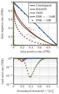
(a) $\rho=0$ dB barrage jammer

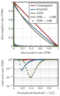
(b) $\rho=10$ dB barrage jammer

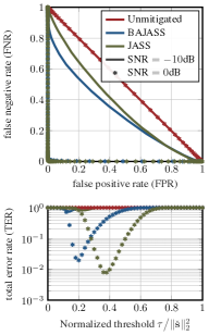
(c) $\rho=30$ dB barrage jammer

Figure 1: Performance against barrage jammers ([inner color=white, fill color= gray, outer color=gray]1) with different transmit powers. The jammers have $I=4$ antennas; the receiver assumes $\hat{I}=4$.

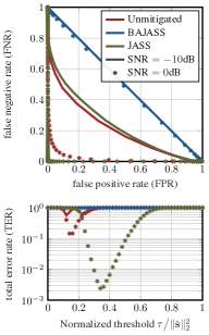
(a) Reactive jammer with $\rho=0$ dB

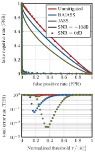
(b) Reactive jammer with $\rho=10$ dB

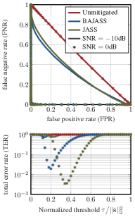
(c) Reactive jammer with $\rho=30$ dB

Figure 2: Performance against reactive jammers ([inner color=white, fill color= gray, outer color=gray]2) with different transmit powers. The jammers have $I=4$ antennas; the receiver assumes $\hat{I}=4$.

In the first experiment, we evaluate the performance of the JASS algorithm and baselines against barrage jammers with $I=4$ antennas (JASS and BAJASS assume $\hat{I}=4$) and different transmit powers, at two different noise levels ($\text{SNR}=-10$ dB and $\text{SNR}=0$ dB). The results are shown in fig:barrage:

At an SNR of $0$ dB, JASS achieves reliable time synchronization regardless of the jammer transmit power: for a sensible choice of $\tau=0.375\|\check{}\mathbf{s}\|_{2}^{2}$, the TER is beneath $1\%$ for all jammer powers. In contrast, the unmitigated baseline has a TER of more than $20\%$ for all $\tau$ even for the weakest jammer and a TER close to $100\%$ for the stronger jammers. The BAJASS baseline identifies the jammer interference with the strongest spatial dimensions of the receive signal, which is a good approximation for strong jammers, but a bad one for weak jammers. In fact, if the jammer’s interference is weak compared to the UE signal, BAJASS will indadvertently null a significant part of the UE receive signal. Thus, we see that BAJASS performs well (but not as good as JASS) against the stronger jammers, but extremely poorly against weaker jammers.

Note that the choice of a good threshold $\tau$ depends on the synchronization method: For unmitigated synchronization and BAJASS, a good threshold is $\tau\approx 0.2\|\check{\mathbf{s}}\|_{2}^{2}$; for JASS, a good threshold is $\tau\approx 0.375\|\check{\mathbf{s}}\|_{2}^{2}$. We also observe that, for the given system dimensions, an SNR of $-10$ dB is too low for reliable synchronization, with the TER remaining significantly above $10\%$ in all cases and for all considered methods.

IV-D2 Performance against reactive jammers

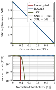
(a) Spoofing jammer [inner color=white, fill color= gray, outer color=gray]3

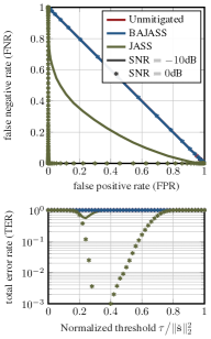
(b) Delayed spoofing jammer [inner color=white, fill color= gray, outer color=gray]4

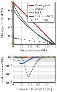
(c) Erratic jammer [inner color=white, fill color= gray, outer color=gray]5

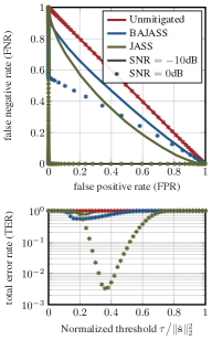
(d) Antenna-switching jammer [inner color=white, fill color= gray, outer color=gray]6

Figure 3: Performance against different jammers with a transmit power of $\rho=30$ dB. All jammers have $I=4$ antennas; the receiver assumes $\hat{I}=4$.

In the second experiment, we evaluate the performance against reactive jammers. We again assume jammers with $I=4$ antennas (JASS and BAJASS assume $\hat{I}=4$) and different transmit powers, at two different noise levels ($\text{SNR}=-10$ dB and $\text{SNR}=0$ dB). The results are shown in fig:onsync:

Overall, the performance is similar to the performance against the barrage jammers from the previous experiment. At an SNR of $-10$ dB, we observe again that reliable synchronization is impossible with all the considered methods—the noise level is simply too high. At an SNR of $0$ dB, unmitigated synchronization performs reasonably well against the weakest jammer, but fails against the stronger jammers. BAJASS performs well (but not as good as JASS) against the stronger jammers, but fails against weak jammers. JASS consistently achieves the best synchronization performance, with a TER of significantly below $1\%$ for all jammer powers when the threshold is set to $\tau=0.375\|\check{\mathbf{s}}\|_{2}^{2}$.

IV-D3 Performance against the other jammers types

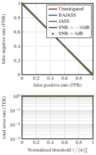
(a) $I=5$, $\hat{I}=4$

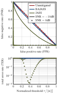
(b) $I=3$, $\hat{I}=4$

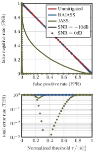
(c) $I=1$, $\hat{I}=4$

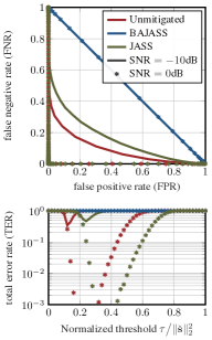
(d) $I=0$, $\hat{I}=4$ (no jammer)

Figure 4: Performance against barrage jammers ([inner color=white, fill color= gray, outer color=gray]1) with a transmit power of $\rho=30$ dB when there is a mismatch between the number of jammer antennas $I$; the receiver’s guess $\hat{I}$ about the number of jammer antennas.

We now consider the performance against the other four jammer types from sec:jammers. In each case, the jammer has $I=4$ antennas and a transmit power of $\rho=30$ dB (JASS and BAJASS assume $\hat{I}=4$). The results are shown in fig:different:

fig:spoofing shows that both the unmitigated method and JASS achieve virtually errorless performance against the spoofing jammer, even at $\text{SNR}=-10$ dB. The reason for this increase in synchronization reliability (compared to the barrage or reactive jammers) is that the spoofing jammer transmits the synchronization sequence simultaneously with the UE, and so can be seen as helping the receiver detect the synchronization sequence at the correct time index $L$. BAJASS, however, fails against the spoofing jammer. The reason for BAJASS’s breakdown is as follows: for the spoofing jammer, when the synchronization sequence is being transmitted ($k\in[L:L+K-1]$), the receive signal can be written as

$$\mathbf{Y}_{L} =\mathbf{h}\check{\mathbf{s}}^{T}+\sqrt{\rho}\mathbf{J}\mathbf{1}_{I}\check{\mathbf{s}}^{T}+\mathbf{N}_{L}$$ (24)

$$=(\mathbf{h}+\sqrt{\rho}\mathbf{J}\mathbf{1}_{I})\check{\mathbf{s}}^{T}+\mathbf{N}_{L},$$ (25)

where $\mathbf{N}_{L}=[\mathbf{n}[L],\dots,\mathbf{n}[L+K-1]]$, and where $\mathbf{h}+\sqrt{\rho}\mathbf{J}\mathbf{1}_{I}$ is a $B\times 1$ matrix. Thus, the receive signal consists only of a rank-one component in the spatial direction of $\mathbf{h}+\sqrt{\rho}\mathbf{J}\mathbf{1}_{I}\in\mathbb{C}^{B}$, plus additive white Gaussian noise. Since BAJASS nulls the $\hat{I}=4$ strongest spatial dimensions of $\mathbf{Y}_{L}$ before measuring the correlation with the synchronization sequence, it will null the spatial subspace $\textit{span}\{\mathbf{h}+\sqrt{\rho}\mathbf{J}\mathbf{1}_{I}\}$ (which dominates the noise subspace due to the strong component from the jammer), as well as three random dimensions of the noise subspace. Since $\textit{span}\{\mathbf{h}+\sqrt{\rho}\mathbf{J}\mathbf{1}_{I}\}$ is the spatial subspace that contains synchronization sequence, its nulling makes it impossible to detect the synchronizaton sequence afterwards.

fig:delayed shows that JASS is the only method that achieves good performance against the delayed spoofing jammer. The unmitigated method fails because the delayed synchronization sequence from the jammer hinders rather than supports the detection of the synchronization sequence at the correct time index $L$. BAJASS fails because the receive signal during the synchronization sequence can now be written as

$$\mathbf{Y}_{L} =\mathbf{h}\check{\mathbf{s}}^{T}+\sqrt{\rho}\mathbf{J}\mathbf{1}_{I}[0,\check{s}_{0},\dots,\check{s}_{K-2}]+\mathbf{N}_{L},$$ (26)

where $\sqrt{\rho}\mathbf{J}\mathbf{1}_{I}$ is a $B\times 1$ matrix. In contrast to the scenario of a spoofing jammer, the jammer does not occupy the same spatial subspace as the UE signal anymore (due to the delay in the spoofed synchronization sequence), but the jammer itself still occupies only a one-dimensional subspace of the receive signal. BAJASS will thus null $\textit{span}\{\sqrt{\rho}\mathbf{J}\mathbf{1}_{I}\}$, as well as the three next strongest dimensions of the receive signal. Since there are no other dimensions that contain jammer interference, the only other dimension that stands out from the spatially uniform thermal noise is the spatial subspace of the UE signal, $\textit{span}\{\mathbf{h}\}$, which will therefore also be nulled (along with two more random dimensions of the noise subspace).

fig:erratic and fig:dynamic show the performance against the erratic jammer and the antenna-switching jammer, respectively. The unmitigated method fails against both jammers. BAJASS performs somewhat better than against the spoofing jammers, but still exhibits a TER of more than $10\%$ (or more than $50\%$, respectively) regardless of the threshold $\tau$. JASS performs well also against these two jammers, with a TER of approximately $1\%$ for a threshold of $\tau=0.375\|\check{\mathbf{s}}\|_{2}^{2}$ (at an SNR of $0$ dB).

IV-D4 Performance under jammer antenna mismatch ($\hat{I}\neq I$)

So far, in all of the previous experiments, JASS and BAJASS have operated using a correct guess $\hat{I}=I=4$ of the jammer’s number of transmit antennas. However, assuming that the receiver knows the exact number of jammer antennas is likely not realistic in practice. Our theoretical result (thm:thm) implies that JASS should work even when $\hat{I}>I$. In this experiment, we therefore evaluate cases where there is a mismatch between the receiver’s guess $\hat{I}$ for the number of jammer antennas and the true number of jammer antennas $I$. The results are shown in fig:mismatch. All jammers are barrage jammers with a transmit power of $\rho=30$ dB.

As expected based thm:thm, JASS performs well when the number of jammer antennas is overestimated (see fig:overestimate_1 and fig:overestimate_2). In contrast, BAJASS fails and achieves a TER close to $100\%$ because it inadvertantly uses the surplus of assumed jammer dimensions to null the UE signal (analogous to the case of the delayed spoofing jammer; cf. sec:different).

In contrast, if the number of jammer antennas is underestimated (fig:underestimate), all methods fail. This failure comes as no surprise: if the number of jammer antennas exceeds the receiver’s estimate, and if the jammer transmits independent interference on all its antennas, then the dimension of the spatial interference subspace exceeds the number of dimensions that are nulled by JASS and BAJASS. As a result, the interference cannot be removed completely by the subspace nulling of JASS and BAJASS. Since a significant part of the jammer interference remains, all methods exhibit a TER of very close to $100\%$, regardless of the threshold $\tau$.

The final case of interest is the case where no jammer is interfering (fig:no_jammer), which can be viewed as a special case of overestimating the number of jammer antennas. Unsurprisingly, the unmitigated method performs well in this scenario. Even in the jammerless scenario, however, the performance of JASS is comparable to that of the unmitigated performance, showing that JASS can also be used in scenarios where it is uncertain if a jamming attack is (or will be) occurring or not. In contrast, BAJASS fails again because it nulls the UE signal (analogous to the case of the delayed spoofing jammer; cf. sec:different).

IV-D5 Results summary

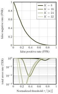
(a) synchronization sequence length $K$​​

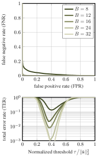
(b) receive antennas $B$

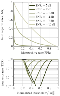
(c) noise power $N_{0}$

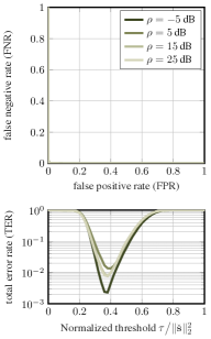
(d) jammer power $\rho$

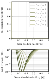
(e) (estimated) jammer antennas $I=\hat{I}$​​​

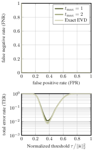
(f) power iterations $t_{\textnormal{max}}$

Figure 5: Ablation studies. Default values are $K=16$, $B=16$, $\textit{SNR}=0\,\text{dB}$, $\rho=30\,\text{dB}$, $I=\hat{I}=4$, $t_{\textnormal{max}}=4$. The jammer is a barrage jammer in all cases.

Our results show that JASS works reliably against all of the considered types of jammers and, at an SNR of $0$ dB achieves a TER of around $1\%$ or less against all jammers (as long as the number of jammer antennas $I$ satisfies $I\leq\hat{I}$). In contrast, the unmitigated method fails against all types of strong jammers except for the spoofing jammer; and BAJASS fails against weak jammers, spoofing jammers, delayed spoofing jammers, erratic jammers, antenna-switching jammers, as well as when the exact number of jammer antennas $I$ is not known, $I\neq\hat{I}$.

We conclude this evaluation by pointing out an advantageous characteristic of JASS. The choice of a good threshold does not depend on the type of jammer; $\tau=0.375\|\check{\mathbf{s}}\|_{2}^{2}$ seems to be a universally good choice for all of the considered jammers. This independence of the threshold to the jammer type is important because, in a real-world scenario, the behavior of an attacking jammer is typically not known in advance.

IV-E Performance of JASS Under Varying System Parameters

After having demonstrated the effectiveness of JASS against different types of jamming attacks, we analyze its performance under varying system parameters. The results are shown in fig:ablation. In each experiment, one system parameter is varied. The system parameters that are held constant for a given experiment are set to the following values: The synchronization sequence length is $K=16$, the number of BS antennas is $B=16$, the noise power $N_{0}$ corresponds to $\text{SNR}=0$ dB, the jammer is a barrage jammer, the jammer transmit power is $\rho=30$ dB, the (estimated) number of jammer antennas is $\hat{I}=I=4$, and the number of power iterations is $t_{\textrm{max}}=4$. In the first experiment, we vary the synchronization sequence length $K$ (see fig:vary_K). Unsurprisingly, the synchronization performance improves with $K$. Note that the value of the optimal threshold $\tau$ changes with $K$ as well. This can easily be taken into account at design time of a system, since the receiver knows $K$.

In the second experiment, we vary the number of receive antennas $B$ (see fig:vary_B). Again, unsurprisingly, the performance improves with $B$. In this case, $B$ appears to have no influence on the choice of the optimal threshold parameter $\tau$.

In the third experiment, we vary the noise power $N_{0}$ by varying the SNR (see fig:vary_SNR). The relation between SNR and $N_{0}$ is described by (20). Naturally, the performance improves as the noise power decreases. Moreover, with decreasing noise power, the optimal threshold parameter moves closer to the optimal objective value $\|\check{\mathbf{s}}\|_{2}^{2}$ from thm:thm.

In the fourth experiment, we vary the jammer transmit power $\rho$ (see fig:vary_rho). As expected based on the discussion in sec:barrage, the performance of JASS does not vary significantly under the jammer transmit power (and neither does the choice of the optimal threshold parameter $\tau$).

In the fifth experiment, we vary the (estimated) number of jammer antennas $I$ and $\hat{I}$ while fixing $I=\hat{I}$ (see fig:vary_I). The performance of JASS improves with decreasing number of jammer antennas. This is due to two reasons: The first reason is that an increased number of the interference dimensions increases the difficulty of the optimization problem in (12), which JASS solves approximately. The second reason is that JASS nulls $\hat{I}$ dimensions of the receive signal, which corresponds to a loss of $\hat{I}$ degrees of freedom (out of $\min\{B,K\}$). The choice of the optimal threshold parameter $\tau$ also varies between the scenarios, though a comparison with the experiment in sec:mismatch indicates that this change is mainly due to the change in $\hat{I}$ (and not due to the change in $I$), which is a parameter that is known at design time of a system.

In the final experiment, we vary the number of power iterations $t_{\textnormal{max}}$ that JASS uses for the eigenvector approximations in alg:power, and we also consider the performance of an exact eigenvalue decomposition (EVD) (see fig:vary_tmax). Naturally, the performance increases with $t_{\textnormal{max}}$, since more iterations lead to more accurate eigenvector approximations. However, we see that already for $t_{\textnormal{max}}=2$ power iterations, the performance is virtually identical to the performance when using an exact EVD.

V Conclusions

We have proposed JASS, the first method for time synchronization that can withstand smart jamming attacks. JASS mitigates jammers using spatial filtering and is based on a novel optimization problem in which a spatial filter is fitted to the time-windowed receive signal to maximize the normalized correlation with the synchronization sequence. We have shown the soundness of the proposed optimization problem in thm:thm, where successful synchronization is guaranteed under some intuitive conditions. The effectiveness of the JASS algorithm itself, which solves this underlying optimization problem only approximately, has been shown via extensive simulations that consider different types jammers.

The extension of our method to frequency-selective channels, as well as the incorporation of frequency synchronization, are left for future work.

Appendix A Proof of thm:thm

Let $\mathbf{A}\in\mathbb{C}^{B\times\hat{I}}$ be any matrix that satisfies $\textit{col}(\mathbf{J})\subseteq\textit{col}(\mathbf{A})$ and $\mathbf{h}\notin\textit{col}(\mathbf{A})$. That such a matrix exists follows from Conditions 2 and 3. For $\tilde{}\mathbf{P}=\mathbf{I}_{B}-\mathbf{A}\mathbf{A}^{H}$ and $\ell=L$, the objective in (10) then equals

$$\frac{\|\tilde{}\mathbf{P}\mathbf{Y}_{\ell}\check{}\mathbf{s}^{\ast}\|_{2}^{2}}{\|\tilde{}\mathbf{P}\mathbf{Y}_{\ell}\|_{F}^{2}}$$

$$=\frac{\|(\mathbf{I}_{B}-\mathbf{A}\mathbf{A}^{H})(\mathbf{h}\check{}\mathbf{s}^{T}+\mathbf{J}[\mathbf{w}[\ell],\dots,\mathbf{w}[\ell\!+\!K\!-\!1])\check{}\mathbf{s}^{\ast}\|_{2}^{2}}{\|(\mathbf{I}_{B}-\mathbf{A}\mathbf{A}^{H})(\mathbf{h}\check{}\mathbf{s}^{T}+\mathbf{J}[\mathbf{w}[\ell],\dots,\mathbf{w}[\ell\!+\!K\!-\!1])\|_{F}^{2}}\!\!$$ (27)

$$=\frac{\left\|(\mathbf{I}_{B}-\mathbf{A}\mathbf{A}^{H})\mathbf{h}\|\check{}\mathbf{s}\|_{2}^{2}\right\|_{2}^{2}}{\|(\mathbf{I}_{B}-\mathbf{A}\mathbf{A}^{H})\mathbf{h}\check{}\mathbf{s}^{T}\|_{F}^{2}}$$ (28)

$$=\frac{\left\|(\mathbf{I}_{B}-\mathbf{A}\mathbf{A}^{H})\mathbf{h}\right\|_{2}^{2}\|\check{}\mathbf{s}\|_{2}^{4}}{\|(\mathbf{I}_{B}-\mathbf{A}\mathbf{A}^{H})\mathbf{h}\|_{2}^{2}\|\check{}\mathbf{s}\|_{2}^{2}}$$ (29)

$$=\|\check{}\mathbf{s}\|_{2}^{2},$$ (30)

where (28) follows from the fact that $(\mathbf{I}_{B}-\mathbf{A}\mathbf{A}^{H})\mathbf{J}=\mathbf{0}$ and that $\check{}\mathbf{s}^{T}\check{}\mathbf{s}^{\ast}=\|\check{}\mathbf{s}\|_{2}^{2}$, and (29) follows from the fact that $\|\gamma\mathbf{a}\|_{2}^{2}=\gamma^{2}\|\mathbf{a}\|_{2}^{2}$ and that $\|\mathbf{a}\mathbf{b}^{T}\|_{F}^{2}=\|\mathbf{a}\|_{2}^{2}\|\mathbf{b}\|_{2}^{2}$.

We now show that the objective in (10) is upper-bounded by $\|\check{}\mathbf{s}\|_{2}^{2}$, and that (with probability one) equality cannot hold if $\ell<L$. From this, the result will directly follow.

That the LHS of (10) is upper-bounded by $\|\check{}\mathbf{s}\|_{2}^{2}$ follows since

$$\frac{\|\tilde{}\mathbf{P}\mathbf{Y}_{\ell}\check{}\mathbf{s}^{\ast}\|_{2}^{2}}{\|\tilde{}\mathbf{P}\mathbf{Y}_{\ell}\|_{F}^{2}} \leq\frac{\|\tilde{}\mathbf{P}\mathbf{Y}_{\ell}\|_{2}^{2}\,\|\check{}\mathbf{s}\|_{2}^{2}}{\|\tilde{}\mathbf{P}\mathbf{Y}_{\ell}\|_{F}^{2}}$$ (31)

$$\leq\|\check{}\mathbf{s}\|_{2}^{2},$$ (32)

where (31) follows from the definition of the spectral norm and (32) follows since the spectral norm is upper bounded by the Frobenius norm.

It remains to show that, with probability one, this upper bound cannot be attained if $\ell<L$. The upper bound is attained if and only if both (32) and (31) hold with equality. Equality in (32) holds if and only if $\tilde{}\mathbf{P}\mathbf{Y}_{\ell}$ is a rank-one matrix. Equality in (31) holds if and only if $\check{}\mathbf{s}$ is collinear with the principal right-singular vector of $\tilde{}\mathbf{P}\mathbf{Y}_{\ell}$ (i.e., the right-singular vector corresponding to the largest singular value). It follows that the upper bound is attained if and only if $\tilde{}\mathbf{P}\mathbf{Y}_{\ell}$ is a rank-one matrix whose only non-degenerate right-singular vector is collinear with $\check{}\mathbf{s}$. Denoting $\mathbf{s}^{T}[\ell-L]=[s[\ell-L],\dots,s[\ell-L+K-1]]$ and $\mathbf{W}_{\ell}=[\mathbf{w}[\ell],\dots,\mathbf{w}[\ell+K-1]]\in\mathbb{C}^{I\times K}$, we can rewrite the windowed receive matrix $\mathbf{Y}_{\ell}$ as

$$\mathbf{Y}_{\ell}=\mathbf{h}\mathbf{s}^{T}[\ell-L]+\mathbf{J}\mathbf{W}_{\ell}=\begin{bmatrix}\mathbf{h}&\mathbf{J}\end{bmatrix}\begin{bmatrix}\mathbf{s}^{T}[\ell-L]\\ \mathbf{W}_{\ell}\end{bmatrix}.$$ (33)

If $\tilde{}\mathbf{P}\mathbf{Y}_{\ell}$ is a rank-one matrix, then its compact singular value decomposition has the form $\mathbf{u}\sigma\mathbf{v}^{H}$, with the right-singular vector $\mathbf{v}$ satisfying $\mathbf{v}^{H}\in\textit{row}([\mathbf{s}^{T}[\ell-L];\mathbf{W}_{\ell}])$.

For any $k=0,\dots,K-1$ the $(k+1)$th column of $\mathbf{W}_{\ell}$ can only depend on the first $k+1$ entries of $\mathbf{s}^{T}[\ell-L]$, which for $\ell<L$ cannot contain $\check{s}_{k^{\prime}},k^{\prime}\geq k$. Since the entries of $\check{}\mathbf{s}$ are i.i.d., it therefore follows that the $(k+1)$th column of $\mathbf{W}_{\ell}$ is independent of $\check{s}_{k^{\prime}},k^{\prime}\geq k$. Moreover, because the entries of $\check{}\mathbf{s}$ are i.i.d., for $\ell<L$, the $(k+1)$th entry of $\mathbf{s}^{T}[\ell-L]$ is independent of $\check{s}_{k^{\prime}},k^{\prime}\geq k$. It follows that, for $\ell<L$ and for all $k=0,\dots,K-1$, the $(k+1)$th column of $[\mathbf{s}^{T}[\ell-L];\mathbf{W}_{\ell}]$ is independent of $\check{s}_{k^{\prime}},k^{\prime}\geq k$. Since the entries of $\check{}\mathbf{s}$ are i.i.d. complex standard Gaussian, it therefore follows that, as long as $I+1<K$ (i.e., as long as the matrix $[\mathbf{s}^{T}[\ell-L];\mathbf{W}_{\ell}]$ is wide), the probability that $\check{}\mathbf{s}^{H}\in\textit{row}([\mathbf{s}^{T}[\ell-L];\mathbf{W}_{\ell}])$ is zero.

It follows that, for any fixed $\ell<L$, the probability that $\check{}\mathbf{s}$ is collinear with $\mathbf{v}$ is zero. And since the union over a countable set of probability-zero events is zero, the probability that there is an $\ell<L$ for which $\check{}\mathbf{s}$ is collinear with $\mathbf{v}$ is zero as well. Hence, with probability one, the upper bound $\|\check{}\mathbf{s}\|_{2}^{2}$ cannot be attained for $\ell<L$ and the result follows. $\blacksquare$

References

- [1] 5G Threat Model Working Panel, “Potential threat vectors to 5G infrastructure,” CISA, NSA, and DNI, May 2021.
- [2] “Satellite-navigation systems such as GPS are at risk of jamming,” The Economist, May 2021.
- [3] “The invisible war in Ukraine being fought over radio waves,” New York Times, Nov. 2023.
- [4] Y. Léost, M. Abdi, R. Richter, and M. Jeschke, “Interference rejection combining in LTE networks,” Bell Labs Tech. J., vol. 17, no. 1, pp. 25–50, Jun. 2012.
- [5] H. Pirayesh and H. Zeng, “Jamming attacks and anti-jamming strategies in wireless networks: A comprehensive survey,” IEEE Commun. Surveys Tuts., vol. 9, no. 2, pp. 767–809, 2022.
- [6] L. M. Hoang, J. A. Zhang, D. N. Nguyen, X. Huang, A. Kekirigoda, and K.-P. Hui, “Suppression of multiple spatially correlated jammers,” IEEE Trans. Veh. Technol., vol. 70, no. 10, pp. 10 489–10 500, Oct. 2021.
- [7] W. Shen, P. Ning, X. He, H. Dai, and Y. Liu, “MCR decoding: A MIMO approach for defending against wireless jamming attacks,” in Proc. IEEE Conf. Commun. Netw. Security (CNS), Oct. 2014, pp. 133–138.
- [8] Q. Yan, H. Zeng, T. Jiang, M. Li, W. Lou, and Y. T. Hou, “Jamming resilient communication using MIMO interference cancellation,” IEEE Trans. Inf. Forensics Security, vol. 11, no. 7, pp. 1486–1499, Jul. 2016.
- [9] G. Marti, T. Kölle, and C. Studer, “Mitigating smart jammers in multi-user MIMO,” IEEE Trans. Signal Process., vol. 71, pp. 756–771, 2023.
- [10] G. Marti and C. Studer, “Joint jammer mitigation and data detection for smart, distributed, and multi-antenna jammers,” in Proc. IEEE Int. Conf. Commun. (ICC), May 2023, pp. 1–6.
- [11] T. T. Do, E. Björnsson, E. G. Larsson, and S. M. Razavizadeh, “Jamming-resistant receivers for the massive MIMO uplink,” IEEE Trans. Inf. Forensics Security, vol. 13, no. 1, pp. 210–223, Jan. 2018.
- [12] G. Marti, O. Castañeda, and C. Studer, “Jammer mitigation via beam-slicing for low-resolution mmWave massive MU-MIMO,” IEEE Open J. Circuits Syst., vol. 2, pp. 820–832, Dec. 2021.
- [13] G. Marti and C. Studer, “Universal MIMO jammer mitigation via secret temporal subspace embeddings,” in Proc. Asilomar Conf. Signals, Syst., Comput., Oct. 2023, pp. 309–316.
- [14] H. Zeng, C. Cao, H. Li, and Q. Yan, “Enabling jamming-resistant communications in wireless MIMO networks,” in Proc. IEEE Conf. Commun. Netw. Security (CNS), Oct. 2017, pp. 1–9.
- [15] X. Jiang, X. Liu, R. Chen, Y. Wang, F. Shu, and J. Wang, “Efficient receive beamformers for secure spatial modulation against a malicious full-duplex attacker with eavesdropping ability,” IEEE Trans. Veh. Technol., vol. 70, no. 2, pp. 1962–1966, Feb. 2021.
- [16] C. Shahriar, M. La Pan, M. Lichtman, T. C. Clancy, R. McGwier, R. Tandon, S. Sodagari, and J. H. Reed, “PHY-layer resiliency in OFDM communications: a tutorial,” IEEE Commun. Surveys Tuts., vol. 17, no. 1, pp. 292–314, 2014.
- [17] Z. Zhang and M. Krunz, “Preamble injection and spoofing attacks in Wi-Fi networks,” in Proc. IEEE Global Commun. Conf. (GLOBECOM), Dec. 2021, pp. 1–6.
- [18] M. J. La Pan, T. C. Clancy, and R. W. McGwier, “Jamming attacks against OFDM timing synchronization and signal acquisition,” in Proc. IEEE Mil. Commun. Conf. (MILCOM), Oct. 2012, pp. 1–7.
- [19] M. Lichtman, R. Jover, M. Labib, R. Rao, V. Marojevic, and J. H. Reed, “LTE/LTE–A jamming, spoofing, and sniffing: threat assessment and mitigation,” IEEE Commun. Mag., vol. 54, no. 4, pp. 54–61, Apr. 2016.
- [20] M. Lichtman, R. Rao, V. Marojevic, J. Reed, and R. P. Jover, “5G NR jamming, spoofing, and sniffing: Threat assessment and mitigation,” in Proc. IEEE Int. Conf. Commun. Workshop (ICCW), May 2018, pp. 1–6.
- [21] M. Eygi and G. K. Kurt, “A countermeasure against smart jamming attacks on LTE synchronization signals,” J. Commun., vol. 15, no. 8, pp. 626–632, Aug. 2020.
- [22] A. El-Keyi, O. Üreten, H. Yanikomeroglu, and T. Yensen, “LTE for public safety networks: synchronization in the presence of jamming,” IEEE Access, vol. 5, pp. 20 800–20 813, 2017.
- [23] M. J. La Pan, M. Lichtman, T. C. Clancy, and R. W. McGwier, “Protecting physical layer synchronization: mitigating attacks against OFDM acquisition,” in Proc. Int. Symp. Wireless Personal Multimedia Commun. (WPMC), 2013, pp. 1–6.
- [24] W. Dinkelbach, “On nonlinear fractional programming,” Management science, vol. 13, no. 7, pp. 492–498, 1967.
- [25] A. Omri, M. Shaqfeh, A. Ali, and H. Alnuweiri, “Synchronization procedure in 5G NR systems,” IEEE Access, vol. 7, pp. 41 286–41 295, 2019.
- [26] Z. Shen, K. Xu, and X. Xia, “Beam-domain anti-jamming transmission for downlink massive MIMO systems: a Stackelberg game perspective,” IEEE Trans. Inf. Forensics Security, vol. 16, pp. 2727–2742, 2021.
- [27] K. Shen and W. Yu, “Fractional programming for communication systems–part I: Power control and beamforming,” IEEE Trans. Signal Process., vol. 66, no. 10, pp. 2616–2630, May 2018.
- [28] R. A. Horn and C. R. Johnson, Matrix Analysis, 2nd ed. Cambridge Univ. Press, 2013.
- [29] C. Eckart and G. Young, “The approximation of one matrix by another of lower rank,” Psychometrika, vol. 1, no. 3, pp. 211–218, 1936.
- [30] L. Mirsky, “Symmetric gauge functions and unitarily invariant norms,” Quart. J. Math, vol. 11, no. 1, pp. 50–59, 1960.