Stochastic Online Optimization for Cyber-Physical and Robotic Systems

Abstract

We propose a novel gradient-based online optimization framework for solving stochastic programming problems that frequently arise in the context of cyber-physical and robotic systems. Our problem formulation accommodates constraints that model the evolution of a cyber-physical system, which has, in general, a continuous state and action space, is nonlinear, and where the state is only partially observed. We also incorporate an approximate model of the dynamics as prior knowledge into the learning process and show that even rough estimates of the dynamics can significantly improve the convergence of our algorithms. Our online optimization framework encompasses both gradient descent and quasi-Newton methods, and we provide a unified convergence analysis of our algorithms in a non-convex setting. We also characterize the impact of modeling errors in the system dynamics on the convergence rate of the algorithms. Finally, we evaluate our algorithms in simulations of a flexible beam, a four-legged walking robot, and in real-world experiments with a ping-pong playing robot.

Keywords: Gradient-Based Stochastic Optimization, Online Learning, Non-Convex Optimization, Reinforcement Learning, Cyber-Physical Systems, Robotic Control

1 Introduction

The increasing availability of sensors across various domains has led to the generation of vast volumes of data, ideal for analysis and training. However, a significant challenge arises from the traditional “Sampling-Training-Deployment” mode of machine learning algorithms. Once trained, most models remain static during deployment, unable to benefit from the continuous influx of new data. This limitation means that models risk becoming outdated as the environment evolves and new information emerges, leaving a substantial amount of potentially valuable data unused. This not only hinders improvements in performance but also falls short of enabling systems to continuously learn, adapt, and improve. Moreover, retraining models from scratch with new data is neither an economical nor a long-term solution. This issue is particularly prevalent in robotics, where deployed models struggle to adapt to ever-changing environments and continuous streams of new information and data.

1.1 Online Learning

In the field of machine learning, a strategy that incorporates streaming data is known as online leaning, which aims to minimize the expected regret as follows (Bubeck, 2012; Neu, 2015):

$$\mathrm{Regret}\left(\mathcal{A}\right)=\mathbb{E}\left[\sum_{t=1}^{T}f\left(\omega_{t};\zeta_{t}\right)\right]-\min_{\omega\in\Omega}\mathbb{E}\left[\sum_{t=1}^{T}f\left(\omega;\zeta_{t}\right)\right],~{}\zeta_{t}\stackrel{{\scriptstyle\text{i.i.d.}}}{{\sim}}\mathcal{D},$$ (1)

where $\mathcal{A}$ denotes the specific online optimization algorithm that is used to minimize the regret and $f$ are stochastic loss functions, where the random variable $\zeta$ is independently and identically sampled from the unknown distribution $\mathcal{D}$. The expectation is taken with respect to the loss functions and the decision variables $\omega_{t}\in\Omega$. The decision variables $\omega_{t}$ are generated by the algorithm $\mathcal{A}$ from a closed and convex set $\Omega\subseteq\mathbb{R}^{n_{\omega}}$, where $n_{\omega}\in\mathbb{N}_{+}$ denotes the number of decision variables $\omega$. The loss functions $f$ are typically assumed to be convex and bounded (Hazan, 2022; Shalev-Shwartz, 2012; Hall and Willett, 2015). However, one of the primary objectives of this article is to bridge the gap between theory and practice, enabling online learning algorithms to be deployed on cyber-physical systems. Therefore, in this article, we abandon the convexity assumption and instead rely on a more general smoothness assumption. In addition, $T$ denotes the total number of iterations. Intuitively, we claim that an online optimization algorithm $\mathcal{A}$ performs well if the regret induced by this algorithm is sub-linear as a function of $T$ (i.e, $\textrm{Regret}\left(\mathcal{A}\right)=o\left(T\right)$), since this implies that on average, the algorithm performs as well as the best fixed decision variables $\omega^{\star}=\arg\min_{\omega\in\Omega}\mathbb{E}\left[\sum_{t=1}^{T}f\left(\omega;\zeta_{t}\right)\right]$ in hindsight. Therefore, when $T$ is large enough or tends to infinity, online learning can cope with continually growing streams of data at the algorithm level, so that the decision variables $\omega_{t}$ continuously improve performance.

Zinkevich (2003) was one of the first researchers to realize that simple gradient-descent strategies are effective at solving (1). Since then, a plethora of online learning algorithms have emerged and their effectiveness has been demonstrated in practical settings. These algorithms can be broadly categorized into two groups: The first group comprises algorithms that are targeted at linear loss functions, also referred to as the prediction with expert advice problem (see Hazan, 2022; Abernethy et al., 2009; Shalev-Shwartz and Singer, 2007), with notable examples being the Follow the Leader (FTL) and Follow the Regularized Leader (FTRL) algorithms, as well as the hedge algorithm (see Freund and Schapire, 1997; Littlestone and Warmuth, 1994; Muehlebach, 2023), and the Perceptron (see Novikoff, 1962). Other online optimization algorithms have also been proposed to tackle the problem of prediction with expert advice, such as the Exponentially Weighted Average Forecaster (EWAF) and the Greedy Forecaster (see Cesa-Bianchi and Lugosi, 2006), as well as the Upper Confidence Bound (UCB) algorithm (see Auer et al., 2002). Compared to these online learning methods that are targeted to linear loss functions, gradient-based methods can handle more general loss functions and sometimes even achieve faster convergence rates (Ruder, 2017). In this article, we will focus on gradient-based online optimization algorithms. Gradients provide local information of the loss functions, which, compared to gradient-free algorithms, is known to expedite the convergence process (Nesterov and Spokoiny, 2017). However, in the stochastic programming problems that are considered herein, gradient information is often challenging or even impossible to obtain, which is why many reinforcement learning algorithms rely, at their core, on zeroth-order optimization. In contrast, we advocate with our work the use of approximate, model-based gradients and demonstrate that even rough estimates are enough to achieve convergence. We also quantitatively characterize the impact of estimation errors on convergence and highlight that in contrast to zeroth-order methods, our rates are dimension independent.

Gradient-based online optimization algorithms can be further categorized based on whether higher-order derivatives are used. Examples of first-order gradient-based algorithms include the Passive-Aggressive Online Learning (see Crammer et al., 2006), the Approximate Large Margin Algorithm (see Gentile, 2000), and the Relaxed Online Maximum Margin Algorithm (see Li and Long, 1999). Among these, the most widely employed algorithm is Online Gradient Descent (OGD) (see Dekel et al., 2012; Hazan et al., 2007b, a; Kolev et al., 2023), which is summarized in Algorithm 1.

Input : initial parameters $\omega_{1}\in\Omega$, iterations $T$, step length $\left\{\eta_{t}\right\}_{t=1}^{T}$

for $t=1$ to $T$ do

       Implementation: play $\omega_{t}$ and observe cost $f_{t}\left(\omega_{t}\right)$;

       Update: $\widehat{\omega}_{t+1}=\omega_{t}-\eta_{t}\nabla f_{t}\left(\omega_{t}\right)$;

       Projection: $\omega_{t+1}=\Pi_{\Omega}\left(\widehat{\omega}_{t+1}\right)$;

      

end for

Return : $\omega_{T+1}$

Algorithm 1 Online Gradient Descent

We note that $\Pi_{\Omega}\left(\cdot\right)$ denotes the projection to the feasible set $\Omega$, and is defined as follows:

$$\omega_{t}=\Pi_{\Omega}\left(\widehat{\omega}_{t}\right)=\operatorname*{arg\,min}_{\omega\in\Omega}\left|\omega-\widehat{\omega}_{t}\right|^{2},$$ (2)

where $\left|\cdot\right|$ denotes the $\ell_{2}$-norm.

Sometimes, even faster convergence rates can be obtained with second-order methods, which not only require gradient information, but also the Hessian (Boyd and Vandenberghe, 2004; Nocedal and Wright, 2006). Examples include the second-order Perceptron (see Cesa-Bianchi et al., 2005), the Confidence Weighted Learning (see Dredze et al., 2008), the Adaptive Regularization of Weight Vectors (see Crammer et al., 2013), and the Online Newton Step Algorithm (see Hazan, 2022). However, in practical applications related to the control of cyber-physical systems, gradients are already difficult to obtain, let alone second-order information. In addition, second-order methods are plagued by the following shortcomings (Martens and Grosse, 2015; Reddi et al., 2019; Bottou, 2010; LeCun et al., 1998; Agarwal et al., 2017a): i) the methods have a high computational complexity per iteration as they require assembling and inverting the Hessian, which is problematic for high-dimensional problems; ii) the methods can be sensitive to noise (inexact gradient and Hessian evaluation), which can result in oscillations or divergence. Thus, in this article, we introduce an efficient approximation method for the Hessian matrix based on a trust-region method. Additionally, we provide a quantitative analysis of the sensitivity of our proposed second-order method to gradient estimation errors.

1.2 Contribution

We note that the methods described above require access to the gradient, which can be easily done in tasks, such as text classification and image classification. However, when applying online learning algorithms to cyber-physical or robotic systems, gradients are usually difficult to obtain. On the one hand, this is due to the often complex dynamics of the cyber-physical system itself, and on the other hand, it is due to the interactions with an environment, which might be unknown or change over time. In addition, some of our common assumptions in online learning settings tend to be ineffective, such as convexity of the loss functions, which often renders the theoretical guarantees vacuous. This also explains why online learning, which has been so successful in machine learning for the last twenty years, has received much less attention in control theory and in applications with cyber-physical systems. The purpose of this article is to address this deficiency. Inspired by Algorithm 1, we propose a gradient-based online learning algorithm that is effective at solving stochastic programming problems related to cyber-physical systems, which we highlight in various simulations and with real-world experiments. We present different means to approximate the gradient, including a random sampling procedure and system identification approaches. We prove convergence of our online learning algorithms in the presence of gradient estimation errors, where we introduce the modeling error modulus $\kappa$ to quantitatively analyze the influence of modeling errors on the convergence. Our main contributions are summarized as follows:

• We introduce a gradient-based online learning algorithm, which encompasses both gradient descent and quasi-Newton methods through an appropriate parameter selection. In this algorithm, both the gradient and the quasi-Hessian matrix rely on approximate first-order gradient estimates. The quasi-Newton method demonstrates invariance to linear transformations of the decision variables, thus offering robustness in step size selection and achieving faster convergence compared to the gradient descent method. In contrast, the gradient descent algorithm has a significantly lower computational complexity per iteration, making it more suitable in conjunction with deep neural networks.

• We prove convergence guarantees of the algorithms without convexity assumptions and rely only on smoothness assumptions. This ensures that our algorithms and conclusions are indeed applicable to a large class of real-world cyber-physical systems. Our convergence analysis requires an argument for decoupling the approximate Hessian matrix from its dependence on past random variables, which provides an important technical contribution.

• We quantitatively analyze the impact of modeling errors on algorithm convergence, which is crucial for ensuring the applicability of our algorithms in real-world cyber-physical systems.

• We establish the connection between our algorithms and real-world cyber-physical systems by learning feedforward and feedback controllers in the classic two-degrees-of-freedom control loop in an online manner. We derive the update schemes for our algorithms in both open-loop and closed-loop systems. Furthermore, the effectiveness of both open-loop and closed-loop approaches is evaluated through numerical experiments.

• We evaluate our conclusions through numerical experiments, simulations, and in real-world experiments. These include a flexible beam, a four-legged walking robot, and a ping-pong playing robot. The ping-pong playing robot is a real-world system that is powered by artificial pneumatic muscles. With our approach, the robotic arm is not only able to continually enhance the tracking performance but also to resist the gradually changing dynamic characteristics of the system over time.

1.3 Related Work

In the context of online learning, when the loss function possesses favorable properties, such as being strongly convex, and the variance of the gradient obtained in each iteration is bounded, the convergence rate of online optimization algorithms can reach $\mathcal{O}\left(\nicefrac{{\ln\left(T\right)}}{{T}}\right)$ (Hazan et al., 2007a). Moreover, Hazan and Kale (2010) pointed out that by using variance reduction even linear convergence rates can be achieved, a sentiment echoed in Rakhlin et al. (2012); Iouditski and Nesterov (2014). If the loss functions fail to be strongly convex, but remain Lipschitz continuous and convex, Zinkevich (2003) has demonstrated that online gradient descent achieves an average regret diminishing as $\mathcal{O}\left(\nicefrac{{1}}{{\sqrt{T}}}\right)$ even if the loss functions are not stochastic but generated by an adversary.

The most typical algorithm for solving stochastic optimization problems is Stochastic Gradient Descent (SGD) (Robbins and Monro, 1951). In the context of large-scale machine learning, SGD is favored over batch algorithms for several reasons: SGD has a lower computational cost per iteration (Bottou et al., 2018), and SGD achieves a faster initial decline (Bertsekas, 2015). Current research is focused on how to reduce the noise in the gradient to enhance the convergence rate of SGD. This concept is evident in algorithms like the Stochastic Variance Reduced Gradient (SVRG) (Johnson and Zhang, 2013), the Stochastic Average Gradient (SAG) (Schmidt et al., 2017), and the Stochastic Average Gradient Accelerated-Descent (SAGA) (Defazio et al., 2014), which reduce the noise in the gradient obtained at each iteration through gradient aggregation without significantly increasing computational effort. The first two methods can achieve a linear convergence rate provided that the loss functions are strongly convex. The latter has been improved upon this basis, enabling it to reach a better convergence rate, still under the condition of strongly convex loss functions. However, these methods typically require traversing all or part of the data set, which is not feasible in the online learning setting.

Johnson and Zhang (2013) pointed out that in standard SGD, the variance of the gradient only diminishes to zero when the step size is reduced to zero, which in turn slows down the convergence rate of the algorithms. Simultaneously, Bottou et al. (2018) highlighted that it is easier for second-order SGD algorithms to tune hyper-parameters in terms of selecting the step size. In this article, we also empirically demonstrate that the step size in SGD requires careful design to ensure convergence, and that our quasi-Newton approach is more robust against non-linearity and ill-conditioning of loss functions. However, second-order algorithms require the loss function to be at least twice differentiable, as they involve computing the Hessian, and the computation can be quite expensive due to the need to calculate its inverse. To address this, researchers have proposed different solutions. One approach is the use of the Hessian-free Newton method: Dembo et al. (1982) developed an algorithm based on conjugate-gradients, which iteratively and inexactly solves the Newton equation (Golub and Loan, 2013), thereby achieving a superlinear convergence rate. Other approaches include the use of subsampling methods to estimate the Hessian (Agarwal et al., 2017b; Byrd et al., 2011; Pilanci and Wainwright, 2017) or quasi-Newton method such as the BFGS (Broyden, 1970; Fletcher, 1970) and the L-BFGS methods (Liu and Nocedal, 1989; Nocedal, 1980). The latter leads to the online L-BFGS method (Mokhtari and Ribeiro, 2014; Schraudolph et al., 2007), which, however, requires computing two subsequent gradients per iteration, a task not easily achievable in the context of online learning. Schraudolph (2001) proposed a second-order stochastic algorithm based on the Gauss-Newton method, which ensures positive semi-definiteness of the estimated Hessian. All these methods can achieve a sublinear convergence rate under suitable conditions.

In comparison, there is significantly less literature on deploying online learning algorithms on cyber-physical systems. Crespi and Ijspeert (2008) used a locomotion controller together with Powell’s method, a gradient-free online optimization method, to optimize the gaits of an amphibious snake robot. The gradient-free online optimization enables fast optimization of the gaits in different media and takes only a few iterations to converge. Cheng and Chen (2014) developed an online parameter optimization method utilizing Gaussian process regression to approximate the relationship between the process parameters and system performance. The proposed online parameter optimization adapts to variations and satisfies the performance requirements. It also demonstrates higher efficiency and accuracy compared to existing methods. Wang et al. (2018) developed an approach based on online optimization for a robot to plan its actions in human-robot collaborations, enabling interactions with complex environments.

Different online optimization algorithms, such as online gradient descent, the online Newton algorithm and online mirror descent (see Hazan, 2022; Bubeck, 2011) have been proposed and convergence results have been established. However, these theoretical proofs rely on the assumption of convexity. This is why, in the control community, there has been a nascent trend under the rubric of feedback optimization (Colombino et al., 2020; Hauswirth et al., 2017; Bernstein et al., 2019), where the steady-state of a cyber-physical system is optimized in an online manner. While the formulation does not measure and characterize regret in the sense of online learning and departs from convexity, it constrains the rate at which the underlying dynamics can change (Colombino et al., 2020) or restricts the interactions of the system with the environment (Hauswirth et al., 2017).

1.4 Structure

This article follows the structure outlined below: In Section 2, we will provide a detailed formulation of the stochastic programming problem addressed in this article. Subsequently, we will propose an algorithmic framework to solve this problem and characterize convergence rates in the presence of modeling errors. We will also discuss the assumptions required for proving the convergence results, whereby the detailed proofs are provided in Appendix B. In Section 3, we will motivate and discuss the proposed algorithms from the perspective of trust-region methods. Section 4 establishes the connection between our algorithms and real-world cyber-physical systems through the classic two-degrees-of-freedom control loop. In addition, we derive the update schemes for our gradient descent algorithm in both open-loop and closed-loop systems. The section highlights the capability of our algorithms to be directly deployed on real-world cyber-physical systems. In Section 5, our algorithms are applied to various cyber-physical and robotic systems, including a flexible beam, a four-legged walking robot and a ping-pong playing robot. The section further analyzes the tightness of our convergence results and the impact of the modeling errors on convergence. The section also provides detailed information about each example and highlights different methods that can be used for estimating gradients. The article concludes with a summary in Section 6.

2 Problem Setting: Stochastic Online Learning

We consider a specific form of (1), which is tailored to cyber-physical and robotic systems. We incorporate the system dynamics through the mapping $G$ and parameterize actions (or control inputs) $u_{t}$ via the function $\pi$. Both the dynamics $G$ as well as the action parameterization $\pi$ are added as constraints. Consequently, (1) is reformulated as follows:

$$\begin{split}&\mathbb{E}_{\zeta_{t}}\left[\sum_{t=1}^{T}l\left(y_{t};\zeta_{t}\right)\right]-\min_{\omega\in\Omega}\mathbb{E}_{\zeta_{t}}\left[\sum_{t=1}^{T}l\left(y_{t}^{\star};\zeta_{t}\right)\right]\\ \mathrm{s.t}.~{}&y_{t}=G\left(s_{0},u_{t};\zeta_{t}\right),~{}y_{t}^{\star}=G\left(s_{0},u_{t}^{\star};\zeta_{t}\right)\\ &u_{t}=\pi\left(\omega_{t},y_{t};\zeta_{t}\right),~{}u_{t}^{\star}=\pi\left(\omega,y_{t}^{\star};\zeta_{t}\right),~{}\zeta_{t}\stackrel{{\scriptstyle\text{i.i.d.}}}{{\sim}}p_{\zeta},\end{split}$$ (3)

where the constraints implicitly define $y_{t}$ as a function of $\omega_{t}$, $s_{0}$ and $\zeta_{t}$, the superscript $\left(\cdot\right)^{\star}$ denotes the optimal value. The implicit equation arises due to the fact that feedback loops may potentially be present, and we assume that $y_{t}$ exists and is well defined. The initial state of the cyber-physical system is denoted by $s_{0}\in\mathcal{S}\subset\mathbb{R}^{n_{s}}$. The vectors $u_{t}=\left(u_{t,1},\dots,u_{t,q}\right)$ and $y_{t}=\left(y_{t,1},\dots,y_{t,q}\right)$ denote the input and output sequences of the cyber-physical system, such as a robot, where $u_{t,i}\in\mathcal{U}\subset\mathbb{R}^{m}$ and $y_{t,i}\in\mathcal{Y}\subset\mathbb{R}^{n},~{}i=1,\dots,q$ represent the input and output at a certain time point $i$ and at iteration $t$ of the learning process. The mapping $G\left(\cdot,\cdot;\zeta\right):\mathcal{S}\times\mathcal{U}^{q}\rightarrow\mathcal{Y}^{q}$ transforms a sequence of inputs into a sequence of outputs and represents the input-output behavior of the cyber-physical system. The input-output behavior is not necessarily deterministic, due to process, measurement, and actuation uncertainty, which is modeled with the random variable $\zeta_{t}$. In practice, the mapping $G$ is typically unknown and may exhibit a high degree of nonlinearity, for example due to friction in the joints of a robot. The mapping $\pi\left(\cdot,y_{t};\zeta\right):\Omega\rightarrow\mathcal{U}^{q}$ describes how the decision variables $\omega_{t}$ affect the controls $u_{t}$. The feasible set $\Omega$ is assumed to be closed and convex, and the function $l\left(\cdot;\zeta\right):\mathcal{Y}^{q}\rightarrow\mathbb{R}$ describes the loss function, for example, tracking error, execution time, energy consumption, etc.

To facilitate understanding for the readers, we use a concrete (but simplified) instance to explain (3). In autonomous driving, the goal is to control a vehicle to avoid unpredictable hazards, such as sharp turns and obstacles, represented by the random variable $\zeta$. The dynamic characteristics of the vehicle are denoted by $G$, while the model $\pi$ is used to generate controls for hazard avoidance. The outputs of the vehicle are represented by $y$, including position, speed, direction, etc. The loss function $l$ evaluates the risk faced in the control attempts to avoid hazards $\zeta$ based on the outputs $y$, with successful avoidance resulting in zero loss. Employing online learning algorithms to solve equation (3) means that we learn the decision variables $\omega$ so that the controls minimize the risks faced in handling various emergency situations in autonomous driving.

Establishing a precise model of $G$ is often a difficult task. Consequently, in this article, we adopt a black-box representation for $G$, avoiding any explicit characterization of its internal dynamics. Although the dynamic characteristics of $G$ are unknown, we assume that $G$ is differentiable with respect to $u$. Furthermore, we adopt the following notational convention: $\mathcal{G}\left(u_{t}\right)$ represents an approximation of the gradient of the mapping $G$ at an input location, more precisely, $\mathcal{G}\left(u_{t}\right)$ denotes an approximation of $\left.\nicefrac{{\partial G\left(s_{0},u;\zeta\right)}}{{\partial u}}\right|_{u=u_{t}}$. In the subsequent sections, we will demonstrate that even a rough approximation of $\left.\nicefrac{{\partial G\left(s_{0},u;\zeta\right)}}{{\partial u}}\right|_{u=u_{t}}$ can serve as valuable prior knowledge, significantly improving the convergence rate of our algorithms.

To address the optimization problem (3), we propose Algorithm 2, which depending on the choice of $\epsilon$ represents either an online gradient descent or an online quasi-Newton method. We note that $\left(\cdot\right)^{\dagger}$ denotes the Moore–Penrose inverse.

Input: initial parameters $\omega_{1}$, constant $\epsilon$ and $\alpha$, iterations $T$, step length $\left\{\eta_{t}\right\}^{T}_{t=1}$

for $t\leftarrow 1$ to $T$ do

       Sampling: $\zeta\sim p_{\zeta}\rightarrow\zeta_{t}$ ;

       Implementation: $G\left(s_{0},\pi\left(\omega_{t},y_{t};\zeta_{t}\right);\zeta_{t}\right)\rightarrow y_{t}$ ;

       Evaluation: $l\left(y_{t};\zeta_{t}\right)$;

       Approximation: $\mathcal{G}\left(u_{t}\right)\approx\nicefrac{{\partial G\left(s_{0},\pi\left(\omega_{t},y_{t};\zeta_{t}\right);\zeta_{t}\right)}}{{\partial u}}$;

       Calculation:

$$\mathcal{L}_{t}=\left(\mathrm{I}-\mathcal{G}\left(u_{t}\right)\frac{\partial\pi\left(\omega_{t},y_{t};\zeta_{t}\right)}{\partial y}\right)^{\dagger}\mathcal{G}\left(u_{t}\right)\frac{\partial\pi\left(\omega_{t},y_{t};\zeta_{t}\right)}{\partial\omega};~{}\rhd\text{approximation of }\frac{\partial y_{t}}{\partial\omega_{t}}$$

$$\Lambda_{t}=\frac{1}{\epsilon}\mathcal{L}_{t}^{\text{T}}\nabla^{2}_{y}l\left(y_{t};\zeta_{t}\right)\mathcal{L}_{t}+\frac{\alpha}{\epsilon}\nabla_{\omega}\pi\left(\omega_{t},y_{t};\zeta_{t}\right)\nabla_{\omega}\pi\left(\omega_{t},y_{t};\zeta_{t}\right)^{\text{T}}+\mathrm{I};$$

$$A_{t}=\frac{1}{t}\sum_{k=1}^{t}\Lambda_{k};$$

Update: $\omega_{t+1}=\omega_{t}-\eta_{t}A_{t}^{\dagger}\mathcal{L}_{t}^{\text{T}}\nabla_{y}l\left(y_{t};\zeta_{t}\right)$ ;

      

end for

Return : $\omega_{T+1}$

Algorithm 2 Online-Quasi Newton Method

In principle, the projection step from Algorithm 1 could be included to ensure that the parameters $\omega_{t}$ remain in $\Omega$. However, in cyber-physical applications, $\pi\left(\omega,y;\zeta\right)$ typically represents a neural network, where the parameters have no direct physical interpretation. Constraints often occur on the inputs $u$, and arise, for example, from actuation limits. These can, however, be addressed by parameterizing the neural network in such a way that input constraints are automatically satisfied. In order to simplify the presentation, we will therefore omit the projection onto $\Omega$, or equivalently set $\Omega:=\mathbb{R}^{n_{\omega}}$. We now summarize the convergence guarantees of Algorithm 2 under the following assumptions:

Assumption 2.1 ($L$-Smoothness)

Let the loss functions $f\left(\cdot;\zeta\right):\Omega\rightarrow\mathbb{R}$ be $L$-smooth, that is,

$$\left|\nabla f\left(v;\zeta\right)-\nabla f\left(\omega;\zeta\right)\right|\leq L\left|v-\omega\right|,$$

for all $\omega,v\in\Omega$.

Assumption 2.2 (Bounded Variance)

There exists a constant $H\geq 0$ such that for all $\omega\in\Omega$ the following inequalities hold:

$$\mathbb{E}_{\zeta}\left[\left|\nabla f\left(\omega;\zeta\right)\right|^{2}\right]\leq H^{2},~{}\mathbb{E}_{\zeta}\left[\left|\mathcal{F}\left(\omega;\zeta\right)\right|^{2}\right]\leq H^{2},$$

where $\mathcal{F}\left(\omega;\zeta\right)$ denotes the estimated gradient of $f\left(\omega;\zeta\right)$ induced by $\mathcal{G}\left(u\right)$, while $\nabla f\left(\omega;\zeta\right)$ denotes the true gradient, that is,

$$\begin{split}&\mathcal{F}\left(\omega;\zeta\right)=\frac{\partial l\left(y;\zeta\right)}{\partial y}\left(\mathrm{I}-\mathcal{G}\left(u\right)\frac{\partial\pi\left(\omega,y;\zeta\right)}{\partial y}\right)^{\dagger}\mathcal{G}\left(u\right)\frac{\partial\pi\left(\omega,y;\zeta\right)}{\partial\omega},\\ &\nabla f\left(\omega;\zeta\right)=\frac{\partial l\left(y;\zeta\right)}{\partial y}\left(\mathrm{I}-\frac{\partial G\left(s_{0},u;\zeta\right)}{\partial u}\frac{\partial\pi\left(\omega,y;\zeta\right)}{\partial y}\right)^{\dagger}\frac{\partial G\left(s_{0},u;\zeta\right)}{\partial u}\frac{\partial\pi\left(\omega,y;\zeta\right)}{\partial\omega}.\end{split}$$

Assumption 2.3 (Bounded Hessian)

Given a sequence of single pseudo-Hessians $\Lambda_{t}$ obtained according to Algorithm 2, there exists a constant $\lambda\geq 1$ such that for all $t=1,\dots,T$ the following inequalities hold:

$$1\leq\lambda_{\mathrm{min}}\left(\Lambda_{t}\right)\leq\lambda_{\mathrm{max}}\left(\Lambda_{t}\right)\leq\lambda,$$

where $\lambda_{\mathrm{min}}$ and $\lambda_{\mathrm{max}}$ denote the minimum and maximum eigenvalues of a matrix, respectively.

In this work, we abandon the convexity assumption of the objective function and employ a more general smoothness assumption instead (see Assumption 2.1). Assumption 2.1 and Assumption 2.2 are standard in non-convex optimization (see Bottou et al., 2018). The matrix $\Lambda_{t}$ in Assumption 2.3 depends on the parameter $\epsilon$, which can always be chosen large enough, such that Assumption 2.3 is satisfied. Beyond this, we also make the following assumption on the modeling errors of our gradient estimate:

Assumption 2.4 (Modeling Error)

Let the parameters $\omega_{t}$ evolve according to Algorithm 2. There exists a constant $\kappa\in\left[0,1\right)$ such that for all $t=1,\dots,T$ the following inequality holds:

$$\left|\mathbb{E}_{\zeta}\left[\left.\mathcal{F}\left(\omega_{t};\zeta\right)\right|\omega_{t}\right]-\mathbb{E}_{\zeta}\left[\left.\nabla f\left(\omega_{t};\zeta\right)\right|\omega_{t}\right]\right|^{2}\leq\frac{\kappa^{2}}{\lambda}\left|\mathbb{E}_{\zeta}\left[\left.\nabla f\left(\omega_{t};\zeta\right)\right|\omega_{t}\right]\right|^{2}.$$ (4)

In fact, the parameter $\lambda$ arises from choosing the $\ell_{2}$-norm in (4). If the inequality (4) is expressed in the metric $\left|\cdot\right|_{A_{t}^{-1}}$, the factor $\nicefrac{{1}}{{\lambda}}$ can be avoided, where $|\cdot|_{A^{-1}_{t}}$ denotes the metric induced by the positive definite matrix $A^{-1}_{t}$, that is,

$$\left|x\right|^{2}_{A^{-1}_{t}}:=\sup_{\left|x\right|\leq 1}x^{\mathrm{T}}A^{-1}_{t}x.$$

Then, we have the subsequent conclusions for Algorithm 2:

Theorem 2.1

Let the loss functions $f\left(\cdot;\zeta\right):\Omega\rightarrow\mathbb{R}$ satisfy Assumption 2.1 and Assumption 2.2, and let the pseudo-Hessian $A_{t}$ satisfy Assumption 2.3. Let the estimate $\mathcal{G}\left(u_{t}\right)$ satisfy Assumption 2.4, and let the step size be chosen as

$$\eta=\sqrt{\frac{2F\left(\omega_{1}\right)}{LH^{2}T}}.$$

Then the following inequality holds:

$$\frac{1}{T}\sum_{t=1}^{T}\mathbb{E}_{\zeta_{1:T}}\left[\left|\nabla F(\omega_{t})\right|^{2}_{A_{t}^{-1}}\right]\leq\sqrt{\frac{2LH^{2}F\left(\omega_{1}\right)}{\left(1-\kappa\right)^{2}T}}+\frac{\lambda H^{2}\left(\ln{T}+2\right)}{\left(1-\kappa\right)T},$$ (5)

where $\omega^{\star}:=\operatorname*{arg\,min}_{\omega\in\Omega}F\left(\omega\right)$ denotes the global optimum and $F\left(\omega\right):=\mathbb{E}_{\zeta}\left[f\left(\omega;\zeta\right)\right]$.

The proof of Theorem 2.1 is included in Appendix B. From the above conclusion, it is evident that even when using approximate gradients and avoiding convexity assumptions, the expected value of the average of the squared gradients still converges at a rate comparable to many popular stochastic optimization algorithms (Bottou et al., 2018). We note that, due to the unavailability of $\nicefrac{{\partial G\left(s_{0},u;\zeta\right)}}{{\partial u}}$ in practical scenarios, the convergence rate of Algorithm 2 needs to be characterized using the modeling error modulus $\kappa$, and the convergence rate is governed by $\nicefrac{{1}}{{1-\kappa}}$. If the modeling error modulus $\kappa$ reaches one, the results become trivial since the right-hand side in (5) becomes arbitrarily large. When the modeling error modulus $\kappa$ is zero, it implies that the estimate $\mathcal{G}\left(u\right)$ has no bias. The intuitive representation of Assumption 2.4 in two-dimensional space is illustrated in Figure 1. The expectation of the gradient estimate $\mathbb{E}_{\zeta}\left[\left.\mathcal{F}\left(\omega_{t};\zeta\right)\right|\omega_{t}\right]$ lies within the open ball with center $\mathbb{E}_{\zeta}\left[\left.\nabla f\left(\omega_{t};\zeta\right)\right|\omega_{t}\right]$ and radius $\nicefrac{{\left|\mathbb{E}_{\zeta}\left[\left.\nabla f\left(\omega_{t};\zeta\right)\right|\omega_{t}\right]\right|}}{{\sqrt{\lambda}}}$. This implies that Assumption 2.4 constrains the estimate $\mathbb{E}_{\zeta}\left[\left.\mathcal{F}\left(\omega_{t};\zeta\right)\right|\omega_{t}\right]$ both in magnitude and direction. Therefore, the parameter $\kappa$ provides a reference for evaluating the quality of the obtained estimates.

Figure 1: This figure illustrates the geometric meaning of the modeling error modulus $\kappa$ in two-dimensional space. The expectation of the gradient estimate $\mathbb{E}_{\zeta}\left[\left.\mathcal{F}\left(\omega_{t};\zeta\right)\right|\omega_{t}\right]$ lies within the open ball with center $\mathbb{E}_{\zeta}\left[\left.\nabla f\left(\omega_{t};\zeta\right)\right|\omega_{t}\right]$ and radius $\nicefrac{{\left|\mathbb{E}_{\zeta}\left[\left.\nabla f\left(\omega_{t};\zeta\right)\right|\omega_{t}\right]\right|}}{{\sqrt{\lambda}}}$.

We observe that by selecting a sufficiently large $\epsilon$, the upper bound $\lambda$ approaches one, thereby transforming Algorithm 2 from a Newton method to a gradient descent method. This suggests that by adjusting the value of $\epsilon$, we can enable the algorithm to switch between Newton and gradient descent methodologies, leading to the following corollary:

Corollary 2.1

Let the assumptions of Theorem 2.1 be satisfied and let $\epsilon\rightarrow+\infty$. Then, the following inequality holds:

$$\frac{1}{T}\sum_{t=1}^{T}\mathbb{E}_{\zeta_{1:T}}\left[\left|\nabla F(\omega_{t})\right|^{2}\right]\leq\sqrt{\frac{2LH^{2}F\left(\omega_{1}\right)}{\left(1-\kappa\right)^{2}T}}+\frac{H^{2}\left(\ln{T}+2\right)}{\left(1-\kappa\right)T}.$$

We note that $A_{t}$ can be interpreted as an approximation of the Hessian matrix. Using its inverse as the metric to measure the norm of the gradient $\nabla F(\omega_{t})$ in (5), guarantees the convergence criteria (and the algorithm) are invariant to linear transformations of the parameters $\omega_{t}$. In the following experiments, we will observe that, compared to the gradient descent method, the quasi-Newton method is better at capturing the local curvature of the objective function, thus achieving more robust convergence and being insensitive to the step size $\eta$.

Next, we will reveal the connection between online learning and stochastic optimization, and provide the corresponding convergence guarantee. Prior to this, we make the following additional assumption:

Assumption 2.5 (Polyak-Łojasiewicz Inequality)

There exists a constant $\mu>0$ such that for all $\omega\in\Omega$, the Polyak-Łojasiewicz (PL) inequality holds:

$$\left|\nabla F\left(\omega\right)\right|^{2}\geq 2\mu\left(F\left(\omega\right)-F\left(\omega^{\star}\right)\right),$$ (6)

where $\omega^{\star}=\operatorname*{arg\,min}_{\omega\in\Omega}F\left(\omega\right)$ denotes the global optimum.

Following this assumption, we have the conclusion:

Corollary 2.2

Let the assumptions in Theorem 2.1 be satisfied, and let Assumption 2.5 hold. Then, for any $\epsilon>0$, the expected regret satisfies the following inequality:

$$\mathbb{E}_{\zeta_{1:T}}\left[\sum_{t=1}^{T}f\left(\omega_{t};\zeta_{t}\right)\right]-\min_{\omega\in\Omega}\mathbb{E}_{\zeta_{1:T}}\left[\sum_{t=1}^{T}f\left(\omega;\zeta_{t}\right)\right]\leq\frac{\hbar_{1}\sqrt{T}+\hbar_{2}\ln{T}+\hbar_{3}}{2\mu},$$ (7)

where

$$\hbar_{1}=\frac{\lambda\sqrt{2LH^{2}F\left(\omega_{1}\right)}}{1-\kappa},~{}\hbar_{2}=\frac{\lambda H^{2}}{1-\kappa},~{}\hbar_{3}=\frac{2\lambda H^{2}}{1-\kappa}.$$

In addition, let $\delta\in\left(0,1\right)$, then the following inequality on the online regret holds with probability $1-\delta$:

$$\sum_{t=1}^{T}f\left(\omega_{t};\zeta_{t}\right)-\min_{\omega\in\Omega}\sum_{t=1}^{T}f\left(\omega;\zeta_{t}\right)\leq\frac{\hbar_{1}\sqrt{T}+\hbar_{2}\ln{T}+\hbar_{3}}{2\mu\delta}.$$ (8)

Proof  We start with (6) and immediately have the following result,

$$\mathbb{E}_{\omega_{1:T}}\left[\sum_{t=1}^{T}\mathbb{E}_{\zeta_{t}}\left[\left.f\left(\omega_{t};\zeta_{t}\right)-f\left(\omega^{\star};\zeta_{t}\right)\right|\omega_{t}\right]\right]\leq\frac{1}{2\mu}\mathbb{E}_{\omega_{1:T}}\left[\sum_{t=1}^{T}\left|\nabla F\left(\omega_{t}\right)\right|^{2}\right]\\ \leq\frac{\lambda}{2\mu}\sum_{t=1}^{T}\mathbb{E}_{\omega_{1:T}}\left[\left|\nabla F(\omega_{t})\right|^{2}_{A^{-1}_{t}}\right],$$

which leads to the following inequality,

$$\mathbb{E}_{\zeta_{1:T}}\left[\sum_{t=1}^{T}f\left(\omega_{t};\zeta_{t}\right)-\sum_{t=1}^{T}f\left(\omega;\zeta_{t}\right)\right]\leq\frac{\hbar_{1}\sqrt{T}+\hbar_{2}\ln{T}+\hbar_{3}}{2\mu},~{}\forall\omega\in\Omega.$$

Then, we have

$$\mathbb{E}_{\zeta_{1:T}}\left[\sum_{t=1}^{T}f\left(\omega_{t};\zeta_{t}\right)\right]-\min_{\omega\in\Omega}\mathbb{E}_{\zeta_{1:T}}\left[\sum_{t=1}^{T}f\left(\omega;\zeta_{t}\right)\right]\leq\frac{\hbar_{1}\sqrt{T}+\hbar_{2}\ln{T}+\hbar_{3}}{2\mu},$$

which proves (7). Next, we apply the Markov inequality and obtain the following result:

$$\sum_{t=1}^{T}f\left(\omega_{t};\zeta_{t}\right)-\min_{\omega\in\Omega}\sum_{t=1}^{T}f\left(\omega;\zeta_{t}\right)\leq\frac{\hbar_{1}\sqrt{T}+\hbar_{2}\ln{T}+\hbar_{3}}{2\mu\delta},$$

which holds with probability $1-\delta$. This concludes the proof of Corollary 2.2.  
The previous results highlight that Algorithm 2 is expected to converge at the standard stochastic rate of $\mathcal{O}\left(\nicefrac{{1}}{{\sqrt{T}}}\right)$ (or equivalently $\mathcal{O}(\sqrt{T})$ regret). The convergence rate is dimension-independent, and the errors in the gradient estimate contribute a factor of $\nicefrac{{1}}{{1-\kappa}}$.

3 Interpretation of Algorithm 2 as Trust-Region Approach

In this section, we will interpret Algorithm 2 from the perspective of a trust-region method. However, we only demonstrate the key steps, while the more detailed derivation is included in Appendix A. For a fixed sample $\zeta$, the loss function $f\left(\omega;\zeta\right)$ and the parameterized network $\pi\left(\omega,y;\zeta\right)$ will be denoted as $f\left(\omega\right)$ and $\pi\left(\omega\right)$ for notational convenience. A trust-region method solves the following transformed optimization problem at each step (Yuan, 2015; Martínez, 1994; Sorensen, 1982):

$$\min_{d\in\Omega}~{} f\left(\omega\right)+\nabla f\left(\omega\right)^{\text{T}}d+\frac{1}{2}d^{\text{T}}\nabla^{2}f\left(\omega\right)d$$

s.t. $$\left|d\right|\leq\Delta,$$

where $\Delta$ denotes the radius of the trust region. Drawing inspiration from this idea, we approximate the loss function locally as follows:

$$\begin{split}M\left(v,\omega\right)=&f\left(\omega\right)+\left(v-\omega\right)^{\text{T}}\mathcal{L}^{\text{T}}\nabla_{y}l\left(y;\zeta\right)+\frac{1}{2}\left(v-\omega\right)^{\text{T}}\mathcal{L}^{\text{T}}\nabla^{2}_{y}l\left(y;\zeta\right)\mathcal{L}\left(v-\omega\right)\\ &+\underbrace{\frac{\alpha}{2}\left|\nabla_{\omega}\pi\left(\omega;\zeta\right)^{\text{T}}\left(v-\omega\right)\right|^{2}}_{\text{Term 1}}+\underbrace{\frac{\epsilon}{2}\left|v-\omega\right|^{2}}_{\text{Term 2}},\end{split}$$ (9)

where

$$\mathcal{L}=\frac{\partial y}{\partial\omega}=\left(\mathrm{I}-\mathcal{G}\left(u\right)\frac{\partial\pi\left(\omega,y;\zeta\right)}{\partial y}\right)^{\dagger}\mathcal{G}\left(u\right)\frac{\partial\pi\left(\omega,y;\zeta\right)}{\partial\omega}.$$

We note that Term $1$ and Term $2$ are used as penalty terms to ensure that when $v\in\Omega$ deviates from the parameters $\omega$, the value of $M\left(v,\omega\right)$ remains strictly greater than that of $f\left(\omega\right)$. Furthermore, these terms help prevent drastic changes in the parameters $\omega$ and their corresponding outputs $u=\pi\left(\omega\right)$ during each iteration of the resulting iterative scheme. In our setting, we can ensure that the trust region constraint is always satisfied, specifically $\left|v-\omega\right|\leq\Delta$, by appropriately adjusting the constant $\epsilon$ in (9).

Next, we calculate the closed-form solution of the minimum point of $\mathbb{E}_{\zeta}\left[\left.M\left(v,\omega\right)\right|\omega\right]$ as follows:

$$\omega^{\star}=\omega-\frac{1}{\epsilon}\left(\Sigma_{1}+\alpha\Sigma_{2}+\text{I}\right)^{-1}\int\mathcal{L}\left(\xi\right)^{\text{T}}\nabla_{y}l\left(y;\xi\right)p_{\zeta}\left(\xi\right)\text{d}\xi,$$ (10)

where

$$\Sigma_{1}=\int\mathcal{L}\left(\xi\right)^{\text{T}}\nabla^{2}_{y}l\left(y;\xi\right)\mathcal{L}\left(\xi\right)p_{\zeta}\left(\xi\right)\text{d}\xi,~{}\Sigma_{2}=\int\nabla_{\omega}\pi\left(\omega;\xi\right)\nabla_{\omega}\pi\left(\omega;\xi\right)^{\text{T}}~{}p_{\zeta}\left(\xi\right)\text{d}\xi,$$

and $\text{I}\in\mathbb{R}^{n_{\omega}\times n_{\omega}}$ denotes the identity matrix. Since the trust-region function $M\left(v,\omega\right)$ provides only a local approximation of the cost function $f\left(\omega\right)$ in the vicinity of the point $\omega$, we adopt the following iterative scheme to guide the parameters $\omega$ towards the optimal value:

$$\omega_{t+1}=\omega_{t}-\frac{1}{\epsilon}\left(\Sigma_{1}+\alpha\Sigma_{2}+\text{I}\right)^{-1}\int\mathcal{L}\left(\xi\right)^{\text{T}}\nabla_{y}l\left(y_{t};\xi\right)p_{\zeta}\left(\xi\right)\text{d}\xi,\quad t=1,\dots,T.$$

In the context of stochastic optimization, where global information is lacking, the matrices $\Sigma_{1}$ and $\Sigma_{2}$ are unavailable. Therefore, we employ the following estimates to respectively replace $\Sigma_{1}$ and $\Sigma_{2}$ for $t=1,\dots,T$:

$$\Sigma_{1}^{t}=\frac{1}{\epsilon t}\sum_{k=1}^{t}\mathcal{L}_{k}^{\text{T}}\nabla^{2}_{y}l\left(y_{k};\zeta_{k}\right)\mathcal{L}_{k},~{}\Sigma_{2}^{t}=\frac{1}{\epsilon t}\sum_{k=1}^{t}\nabla_{\omega}\pi\left(\omega_{k},y_{k};\zeta_{k}\right)\nabla_{\omega}\pi\left(\omega_{k},y_{k};\zeta_{k}\right)^{\text{T}},$$

Likewise, we replace the term $\int\mathcal{L}\left(\xi\right)^{\text{T}}\nabla_{y}l\left(y_{t};\xi\right)p_{\zeta}\left(\xi\right)\text{d}\xi$ with the estimate $\mathcal{L}_{t}^{\text{T}}\nabla_{y}l\left(y_{t};\zeta_{t}\right)$. Finally, we introduce the step size $\eta_{t}$ at each iteration and get the following iterative scheme:

$$\omega_{t+1}=\omega_{t}-\eta_{t}\left(\Sigma_{1}^{t}+\alpha\Sigma_{2}^{t}+\text{I}\right)^{-1}\mathcal{L}_{t}^{\text{T}}\nabla_{y}l\left(y_{t};\zeta_{t}\right).$$ (11)

We note that in (11), the term $\nabla_{y}l\left(y_{t};\zeta_{t}\right)$ can be easily obtained at each iteration by observing the output of the cyber-physical system. Meanwhile, $\Sigma^{t}_{2}$ can be obtained by performing backpropagation at each iteration. Therefore, the only term that is difficult to obtain accurately in Algorithm 2 is the gradient $\mathcal{L}_{t}$ and the corresponding $\Sigma^{t}_{1}$. Therefore, we use the approximate gradient $\mathcal{G}\left(u\right)$ instead of $\nicefrac{{\partial G\left(s_{0},u;\zeta\right)}}{{\partial u}}$.

4 Connection to Cyber-Physical Systems and Robotics

In this article, we not only emphasize the importance of convergence analysis but also bridge the gap between theory and practical cyber-physical systems. From the analysis in Section 2 we conclude that as long as the approximate gradient $\mathcal{G}\left(u_{t}\right)$ is accurate enough (as characterized by the error modulus $\kappa$) convergence is guaranteed and Algorithm 2 can be directly deployed on a cyber-physical system. We note that for cyber-physical systems, common estimation methods include system identification and finite difference estimation (Ljung, 2010; Pintelon and Schoukens, 2012; Carè et al., 2018; Tsiamis and Pappas, 2019; Campi and Weyer, 2002). In the following examples, we will use these estimation methods to demonstrate the broad applicability and robustness (insensitivity to modeling errors) of our algorithm.

First of all, we endow the random variable $\zeta$ with a specific meaning for cyber-physical systems. In the following sections of this article, we consider the random variable $\zeta$ as the reference trajectory $y_{\mathrm{ref}}\in\mathcal{Y}^{q}$ that the system is required to track. Given that the learning task is trajectory tracking, an intuitive choice for the loss function $l$ is the deviation from the reference trajectory, that is,

$$l\left(y_{t};y_{\text{ref},t}\right):=\frac{1}{2}\left|G\left(s_{0},u_{t};y_{\text{ref},t}\right)-y_{\text{ref},t}\right|^{2},~{}y_{\text{ref},t}\stackrel{{\scriptstyle\text{i.i.d.}}}{{\sim}}p_{y_{\text{ref}}},~{}t=1,\dots,T.$$ (12)

Thereby, we have $\nabla^{2}_{y}l\left(y;\zeta\right)=\mathrm{I}$. As delineated in (1), $t$ denotes the current iteration, with the total iterations denoted by $T$. This notation inherently suggests that the reference trajectory $y_{\text{ref}}$ evolves in correspondence with the progression of iterations. Concurrently, at each iteration, the reference trajectory is randomly sampled from a fixed yet unknown distribution $p_{y_{\text{ref}}}$. The distribution $p_{y_{\text{ref}}}$ depends upon the specific robotic task at hand, with trajectory tracking serving as a broad, universal objective. For example, in the context of training a robot for table tennis, $p_{y_{\text{ref}}}$ is determined by the trajectories experienced by the end-effector during ball interception (Ma et al., 2022, 2023; Tobuschat et al., 2023). Given the specific meaning of $\zeta$ and the action parameterization $\pi$, implies that we have identified a nonlinear feedforward and feedback controller that yields accurate trajectory tracking for any $y_{\text{ref}}\sim p_{y_{\text{ref}}}$ when solving (3). For simplification and without really compromising generality (we could extend the function $\pi$ to also account for $s_{0}$), we assume that the system consistently initializes from an identical state prior to each iteration. As such, the initial state $s_{0}$ can be fixed and omitted. For example, in the experiments with the ping-pong robot we drive the robot back to a rest position after each iteration of the online learning with a simple proportional-integral-derivative (PID) controller.

To address the learning tasks in cyber-physical systems, we draw inspiration from the classical two-degrees-of-freedom control framework, which includes a feedforward block and a feedback block, and is shown in Figure 2(a). The two-degrees-of-freedom control loop has extensive applications in machine learning within the context of robotics. We can contrast our approach of learning feedforward and feedback controllers to reinforcement learning (RL), where the objective is to learn a feedback controller (policy) that minimizes a designated reward function (Sutton and Barto, 2018; Li, 2018). In contrast to RL, which is often based on approximately solving the Bellman equation, we do not use any dynamic programming strategy in our approach.

(a) two-degrees-of-freedom control loop

(b) feedforward control loop

Figure 2: The figure shows the classical two-degrees-of-freedom control framework in panel (a), which includes a feedforward controller and a feedback controller, and a pure feedforward control framework in panel (b). The variable $n_{\text{d}}$ denotes a disturbance, which will subsequently be used to obtain an approximate gradient $\mathcal{G}\left(u_{t}\right)$.

In our approach, we use $\pi_{\text{ff}}$ and $\pi_{\text{fb}}$ to represent the parameterized feedforward and feedback networks, respectively, and $\omega_{\text{ff}}$ and $\omega_{\text{ff}}$ to denote their corresponding parameters. Then, the relation between $y_{t}$ and $u_{t}$ in (3) can be reformulated as follows:

$$\begin{split}&y_{t}=G\left(s_{0},u_{t};\zeta_{t}\right)\\ &u_{t}=\pi_{\text{ff}}\left(\omega_{\text{ff},t};\zeta_{t}\right)+\pi_{\text{fb}}\left(\omega_{\text{fb},t};y_{t}-\zeta_{t}\right),~{}\zeta_{t}\stackrel{{\scriptstyle\text{i.i.d.}}}{{\sim}}p_{\zeta},\end{split}$$ (13)

that is, the input $u_{t}$ is the combination of a feedforward part $\pi_{\text{ff}}$ that does not depend on $y_{t}$ and a feedback part $\pi_{\text{fb}}$ that depends on the deviation of $y_{t}$ from the reference trajectory $\zeta_{t}$. Due to the inclusion of feedback $\pi_{\text{fb}}$, the calculation of the gradient in Algorithm 2 becomes more complex and less intuitive compared to the open-loop situation where $\pi_{\text{fb}}=0$. Hence, we will demonstrate the computation of the gradients $\nicefrac{{\partial y}}{{\partial\omega_{\text{ff}}}}$ and $\nicefrac{{\partial y}}{{\partial\omega_{\text{fb}}}}$ in the closed-loop system and discuss their implications. The critical aspect to note at this point is that (13) defines an implicit equation for $y_{t}$ and also $u_{t}$. We should therefore think of $y_{t}$ and $u_{t}$ as functions of $\omega_{\text{ff}}$, $\omega_{\text{fb}}$ and $\zeta_{t}$, that is, $u=u\left(\omega_{\text{ff}},\omega_{\text{fb}};\zeta\right)$, $y=y\left(\omega_{\text{ff}},\omega_{\text{fb}};\zeta\right)$. The gradient of the loss function $f$ with respect to the parameters can be calculated as follows:

$$\nabla_{\omega}f\left(\omega;\zeta\right)=\begin{bmatrix}\frac{\partial y^{\text{T}}}{\partial\omega_{\text{ff}}}&\frac{\partial y^{\text{T}}}{\partial\omega_{\text{fb}}}\end{bmatrix}\nabla_{y}l\left(y;\zeta\right).$$

By combining the two equations in (13) we get a single implicit equation for $y$. The differential $\nicefrac{{\partial y}}{{\partial\omega_{\text{ff}}}}$ can now be obtained by differentiating the implicit equation with respect to $\omega_{\text{ff}}$ (implicit function theorem):

$$\begin{split}\frac{\partial y}{\partial\omega_{\text{ff}}}=&\left.\frac{\partial G\left(u;\zeta\right)}{\partial u}\right|_{u=\pi_{\text{ff}}+\pi_{\text{fb}}}\left.\frac{\partial\pi_{\text{fb}}\left(\omega_{\text{fb}};\zeta^{\circ}\right)}{\partial\zeta^{\circ}}\right|_{\zeta^{\circ}=G\left(u;\zeta\right)-\zeta}\frac{\partial y}{\partial\omega_{\text{ff}}}\\ &+\left.\frac{\partial G\left(u;\zeta\right)}{\partial u}\right|_{u=\pi_{\text{ff}}+\pi_{\text{fb}}}\frac{\partial\pi_{\text{ff}}\left(\omega_{\text{ff}};\zeta\right)}{\partial\omega_{\text{ff}}}.\end{split}$$

This can be rearranged to

$$\frac{\partial y}{\partial\omega_{\text{ff}}}=\left(\mathrm{I}-\frac{\partial G\left(u;\zeta\right)}{\partial u}\left.\frac{\partial\pi_{\text{fb}}\left(\omega_{\text{fb}};\zeta^{\circ}\right)}{\partial\zeta^{\circ}}\right|_{\zeta^{\circ}=G\left(u;\zeta\right)-\zeta}\right)^{\dagger}\frac{\partial G\left(u;\zeta\right)}{\partial u}\frac{\partial\pi_{\text{ff}}\left(\omega_{\text{ff}};\zeta\right)}{\partial\omega_{\text{ff}}}.$$ (14)

The expression $\nicefrac{{\partial y}}{{\partial\omega_{\text{fb}}}}$ can be derived with a similar argument and results in

$$\frac{\partial y}{\partial\omega_{\text{fb}}}=\left(\mathrm{I}-\frac{\partial G\left(u;\zeta\right)}{\partial u}\left.\frac{\partial\pi_{\text{fb}}\left(\omega_{\text{fb}};\zeta^{\circ}\right)}{\partial\zeta^{\circ}}\right|_{\zeta^{\circ}=G\left(u;\zeta\right)-\zeta}\right)^{\dagger}\frac{\partial G\left(u;\zeta\right)}{\partial u}\left.\frac{\partial\pi_{\text{fb}}\left(\omega_{\text{fb}};\zeta^{\circ}\right)}{\partial\omega_{\text{fb}}}\right|_{\zeta^{\circ}=G\left(u;\zeta\right)-\zeta}.$$ (15)

We observe that the term $\nicefrac{{\partial G\left(u;\zeta\right)}}{{\partial u}}$ consistently represents the gradient of the open-loop system and, as previously mentioned, can be approximated using the estimate $\mathcal{G}\left(u\right)$. This approximation renders the terms $\nicefrac{{\partial y}}{{\partial\omega_{\text{ff}}}}$ and $\nicefrac{{\partial y}}{{\partial\omega_{\text{fb}}}}$ computable. We also note that the feedback controller may reduce the effect of estimation errors in $\mathcal{G}$ on the resulting gradient estimates $\mathcal{F}$. Indeed, if $\nicefrac{{\partial\pi_{\text{fb}}\left(\omega_{\text{fb}};\zeta^{\circ}\right)}}{{\partial\zeta^{\circ}}}$ is large, both expressions reduce to

$$\frac{\partial\pi_{\text{fb}}\left(\omega_{\text{fb}};\zeta^{\circ}\right)^{\dagger}}{\partial\zeta^{\circ}}\frac{\partial\pi_{\text{fb}}\left(\omega_{\text{fb}};\zeta^{\circ}\right)}{\partial\omega_{\text{fb}}},~{}\frac{\partial\pi_{\text{fb}}\left(\omega_{\text{fb}};\zeta^{\circ}\right)^{\dagger}}{\partial\zeta^{\circ}}\frac{\partial\pi_{\text{ff}}\left(\omega_{\text{ff}};\zeta\right)}{\partial\omega_{\text{ff}}},$$

respectively, which means that $\nabla f$ is approximately independent of $G$ for large $\nicefrac{{\partial\pi_{\text{fb}}\left(\omega_{\text{fb}};\zeta^{\circ}\right)}}{{\partial\zeta^{\circ}}}$. If the feedback gain is small, however, $\nicefrac{{\partial y}}{{\partial\omega_{\text{ff}}}}$ and $\nicefrac{{\partial y}}{{\partial\omega_{\text{fb}}}}$ reduce to

$$\frac{\partial G\left(s_{0},u;\zeta\right)}{\partial u}\frac{\pi_{\text{ff}}\left(\omega_{\text{ff}};\zeta\right)}{\partial\omega_{\text{ff}}},~{}\frac{\partial G\left(s_{0},u;\zeta\right)}{\partial u}\frac{\pi_{\text{fb}}\left(\omega_{\text{fb}};\zeta^{\circ}\right)}{\partial\omega_{\text{fb}}}.$$

Moving forward, we will briefly show that the term

$$\left(\mathrm{I}-\frac{\partial G\left(u;\zeta\right)}{\partial u}\frac{\partial\pi_{\text{fb}}\left(\omega_{\text{fb}};\zeta^{\circ}\right)}{\partial\zeta^{\circ}}\right)^{\dagger}\frac{\partial G\left(u;\zeta\right)}{\partial u}$$ (16)

is the gradient of the closed-loop system with respect to the external input $n_{\text{d}}$ (see Figure 2). This finding enables us to directly derive gradient estimation approaches for the closed-loop system, which will be denoted as $\mathcal{G}^{\circ}\left(\omega_{\text{ff}},\omega_{\text{fb}},\zeta\right)$. We perform the following calculations (implicit function theorem):

$$\frac{\partial y}{\partial n_{\text{d}}}=\left.\frac{\partial G\left(u;\zeta\right)}{\partial u}\right|_{u=\pi_{\text{ff}}+\pi_{\text{fb}}}\left.\frac{\partial\pi_{\text{fb}}\left(\omega_{\text{fb}};\zeta^{\circ}\right)}{\partial\zeta^{\circ}}\right|_{\zeta^{\circ}=G\left(u;\zeta\right)-\zeta}\frac{\partial y}{\partial n_{\text{d}}}+\left.\frac{\partial G\left(u;\zeta\right)}{\partial u}\right|_{u=\pi_{\text{ff}}+\pi_{\text{fb}}},$$

which results in

$$\frac{\partial y}{\partial n_{\text{d}}}=\left(\mathrm{I}-\frac{\partial G\left(u;\zeta\right)}{\partial u}\frac{\partial\pi_{\text{fb}}\left(\omega_{\text{fb}};\zeta^{\circ}\right)}{\partial\zeta^{\circ}}\right)^{\dagger}\frac{\partial G\left(u;\zeta\right)}{\partial u}.$$

Intuitively, $\nicefrac{{\partial y}}{{\partial n_{\text{d}}}}$ describes the sensitivity of $y$ in closed-loop to changes in $u$.

Consequently, the terms $\nicefrac{{\partial y}}{{\partial\omega_{\text{ff}}}}$ and $\nicefrac{{\partial y}}{{\partial\omega_{\text{fb}}}}$, apart from being derived from (14) and (15), can also be obtained through the following more direct approach

$$\frac{\partial y}{\partial\omega_{\text{ff}}}=\mathcal{G}^{\circ}\left(\omega_{\text{ff}},\omega_{\text{fb}},\zeta\right)\frac{\partial\pi_{\text{ff}}\left(\omega_{\text{ff}};\zeta\right)}{\partial\omega_{\text{ff}}},~{}\frac{\partial y}{\partial\omega_{\text{fb}}}=\mathcal{G}^{\circ}\left(\omega_{\text{ff}},\omega_{\text{fb}},\zeta\right)\frac{\partial\pi_{\text{fb}}\left(\omega_{\text{fb}};\zeta^{\circ}\right)}{\partial\omega_{\text{fb}}},$$

thereby allowing for direct computations if $\mathcal{G}^{\circ}$ is known. As we will highlight with simulation experiments $\mathcal{G}^{\circ}\left(\omega_{\text{ff}},\omega_{\text{fb}},\zeta\right)$ can be computed directly by performing stochastic rollouts with different random perturbations $n_{\text{d}}$ (see Section 5.2).

5 Experiments

In this section, we will demonstrate the effectiveness of our algorithms through extensive experiments conducted on various cyber-physical systems, including simulation and real-world experiments. Additionally, we evaluate the accuracy of the theoretical convergence rate of the algorithm proposed in Section 2. In each experiment, we will first introduce the underlying cyber-physical system. Then, based on the specific systems, we will describe the distribution of the reference trajectories, the structure of the parameterized models $\pi$, and the corresponding structure of the inputs. We highlight that even shallow networks work well with our algorithms. Depending on different scenarios, we will employ an appropriate method to obtain gradient estimates $\mathcal{G}\left(u\right)$ and $\mathcal{G}^{\circ}$. Finally, we will discuss the results of the experiments in terms of convergence rate and robustness to modeling errors. It is worth mentioning that the primary intention of the following experiments is not to outperform any existing (reinforcement) learning algorithms but to evaluate the effectiveness of our algorithms and offer another possibility for the development of machine learning in the field of robotics.

5.1 Cantilever Beam

The first example is based on the control of a flexible cantilever beam. The example illustrates how our approach can easily handle dynamical systems with a large number of hidden states (here $100$). We note that current reinforcement learning algorithms have difficulties in dealing with continuous state and action spaces exceeding two dozen states. Modeling and controlling flexible structures has numerous engineering applications (Shabana, 1997; Amirouche, 2007), such as active vibration control of wind turbines, aircraft wings or turbo generator shafts. We consider a cantilever beam illustrated in Figure 3, where the left end of the beam is hinged to a joint, and the active torque $\tau$ is applied only at the left end to counteract the disturbances at the tip of the flexible body. The total length of the entire cantilever beam in a rest configuration is denoted by $l$.

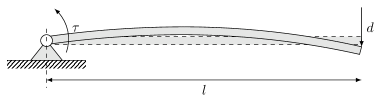
Figure 3: Deformation of the cantilever beam under the active torque and an external disturbance $d$, where the dashed line represents the position of the cantilever beam when at rest.

We employ a lumped-parameter method to discretize the cantilever beam, as illustrated in Figure 4, into a collection of $n$ rigid units.

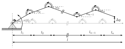
Figure 4: The figure depicts the discrete model of the cantilever beam obtained using the lumped-parameter method. The entire beam is decomposed into $n$ rigid units, with adjacent units interconnected by a pair of spring and damper. Each rigid unit has a length of $l_{i}$, and the angle it makes with the horizontal plane is denoted by $\alpha_{i}$. The active torque is applied only to the first rigid unit hinged to the wall. The gray object indicates the position of the beam when at rest.

In the discrete model of the cantilever beam, the entire beam is divided into $n$ rigid units, either uniformly or non-uniformly. These rigid units are coupled through joints equipped with internal springs and dampers. The joints provide the degrees of freedom required for deformation. The mass, spring, and damper elements offer inertial, restorative, and dissipative forces, respectively, which collectively account for the deformation. Typically, due to the small deformation assumption, the springs and dampers inside each joint are considered linear. In this experiment, however, we will explore the performance of our algorithms in nonlinear systems. Therefore, we adjust the parameters of the cantilever beam (such as the moment of inertia and damping parameters) to enable large deformations and introduce the following nonlinear spring force:

$$f_{\mathrm{spring},i}\left(\Delta\alpha_{i}\right)=k_{i1}\Delta\alpha_{i}+k_{i2}\Delta\alpha_{i}^{3}+k_{i3}\Delta\alpha_{i}^{5},~{}i=1,\dots,n,$$

where $\Delta\alpha_{i}:=\alpha_{i}-\alpha_{i-1}$ represents the angular difference between two adjacent rigid units, and $\alpha_{0}=$0$$. The sole active torque is applied to the first rigid unit. All specific parameters used in this experiment are summarized in Table 1. The following experiments are implemented in Matlab and Simulink.

parameter	value	unit	description
$n$	$50$	-	number of rigid units
$l_{i}$	$3\text{\times}{10}^{-2}$	$\unit{}$	length of each rigid unit
$I_{\mathrm{A}}$	$5\text{\times}{10}^{-3}$	$\unit{{}^{4}}$	the moment of inertia
$k_{i1}$	$5$	N.m/rad	spring coefficient
$k_{i2}$	$1\text{\times}{10}^{3}$	N.m/rad^3	spring coefficient
$k_{i3}$	$1\text{\times}{10}^{4}$	N.m/rad^5	spring coefficient
$b_{i}$	$30$	N.s/rad	damper coefficient

Table 1: Parameters of the discrete beam model.

5.1.1 Reference Trajectory Distribution

The aim of this experiment is to utilize Algorithm 2 to learn the parameterized networks $\pi_{\text{ff}}$ and $\pi_{\text{fb}}$ in an online manner (see Figure 2). The outputs of the parameterized networks yield the active torque $\tau$. The aim of the online learning is to find the parameters $\omega_{\text{ff}}$ and $\omega_{\text{fb}}$, in order to minimize the tracking error of the end-effector ($\left|y-y_{\text{ref}}\right|$) for reference trajectories sampled from the unknown distribution $p_{y_{\text{ref}}}$. The output $y$ describes the distance in $y$-direction between the tip of the beam and the horizontal plane. We observe that the presence of nonlinear spring forces and large deformations, coupled with as many as $100$ hidden states (position and velocity in $y$-direction of each unit), renders this task highly challenging.

All reference trajectories used in the experiment arise from sampling an unknown but fixed distribution. At each iteration, we randomly generate the reference trajectory based on the following principles: 1. Over a time span of $T_{\text{sim}}$ seconds, the trajectory starts from rest and eventually returns to its initial position, and remains still for an additional $\qty{0.5}{}$. 2. Apart from the starting and ending points ($y_{0}$ and $y_{T}$), two other time points, $t_{a}$ and $t_{b}$, will be randomly selected within the time duration $T_{\text{sim}}$. The displacements ($y_{a}$ and $y_{b}$) and velocities ($v_{a}$ and $v_{b}$) at these moments will also be randomly generated, with the accelerations being set to zero. 3. The four points are connected using trajectories that minimize jerk (Geering, 2007; Piazzi and Visioli, 1997). The values of the various parameters are summarized in Table 2.

parameter	unit	distribution	range
$t_{a}$	$\unit{}$	uniformly distributed	$\left[1.2,1.8\right]$
$t_{b}$	$\unit{}$	uniformly distributed	$\left[2.9,3.5\right]$
$y_{a}$, $y_{b}$	$\unit{}$	uniformly distributed	$\left[-0.2,0.2\right]$
$v_{a}$, $v_{b}$	$\unit{m/s}$	uniformly distributed	$\left[-2.0,2.0\right]$

Table 2: Summary of the parameters used for generating reference trajectories.

Figure 5 illustrates the sampling procedure for the reference trajectories along with $400$ samples. The total duration is set to $T_{\text{sim}}=\qty{5.5}{}$. The red dashed boxes indicate the spatial and temporal distribution range of the points $y_{a}$ and $y_{b}$, respectively. We observe that the range of the trajectory is extensive and is not limited to small deformations. In the subsequent experiments, we will see that the parameterized networks trained by our algorithms effectively generalize well across the entire support of $p_{y_{\text{ref}}}$.

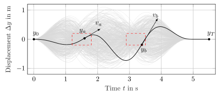
Figure 5: The figure illustrates the range of reference trajectories used for training, where the gray lines are composed of $400$ randomly sampled reference trajectories. The red dashed boxes indicate the spatial and temporal distribution range of the points $y_{a}$ and $y_{b}$, respectively.

5.1.2 Gradient Estimation

As mentioned in Section 3, most of the terms required by Algorithm 2 can be obtained through measurement and computation. However, since the system $G$ is treated as a black-box model, the gradient of the system $\nicefrac{{\partial G\left(s_{0},u;\zeta\right)}}{{\partial u}}$ cannot be analytically determined. To address this, in this numerical experiment, we employ system identification in the frequency domain to obtain a rough linear estimate of $\nicefrac{{\partial G\left(s_{0},u;\zeta\right)}}{{\partial u}}$ (Pintelon and Schoukens, 2012). We excite the discrete model in Simulink with an excitation signal ranging from $\qtyrange{0}{4}{}$, with an interval of $\qty{0.1}{}$. The resulting system response in the frequency domain and the estimated linear transfer function are shown in Figure 6. Next, we use the obtained transfer function to construct a linear approximation of $\nicefrac{{\partial G\left(s_{0},u;\zeta\right)}}{{\partial u}}$, which is denoted by $\mathcal{G}$. It is important to emphasize that in this case the gradient estimate $\mathcal{G}$ is static, meaning that it does not change as a function of $u$. For the specific construction method, please refer to Ma et al. (2022, 2023). We observe that the system exhibits a high degree of nonlinearity, which is reflected by the fact that the uncertainty (residual of the linear model) is dominated by the nonlinearities $\sigma_{\text{nonlinear}}$.

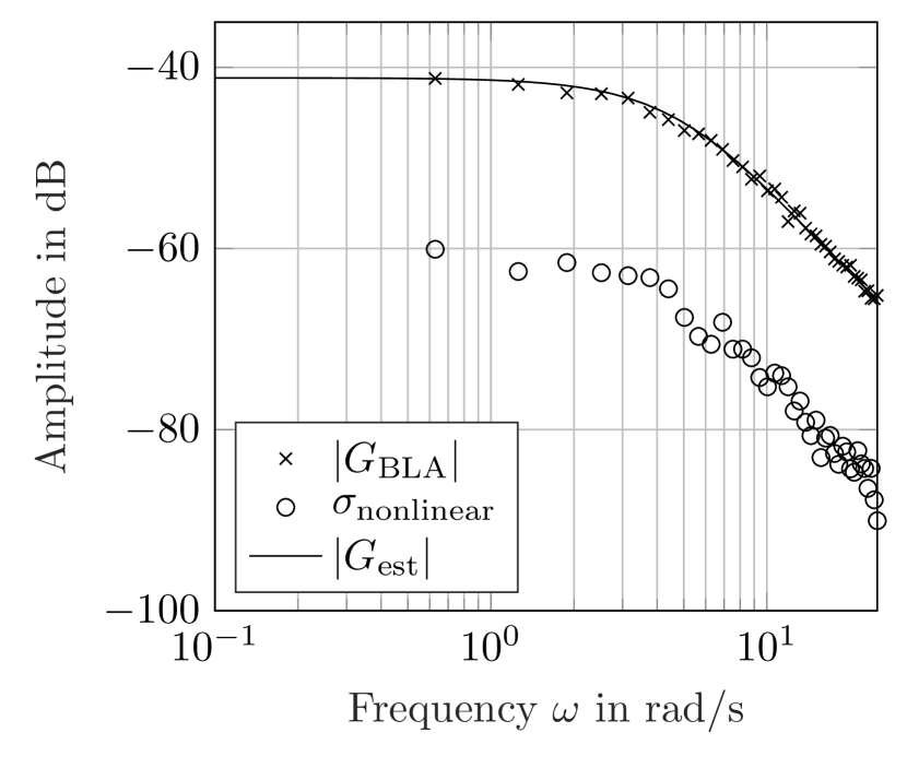
(a) amplitude diagram

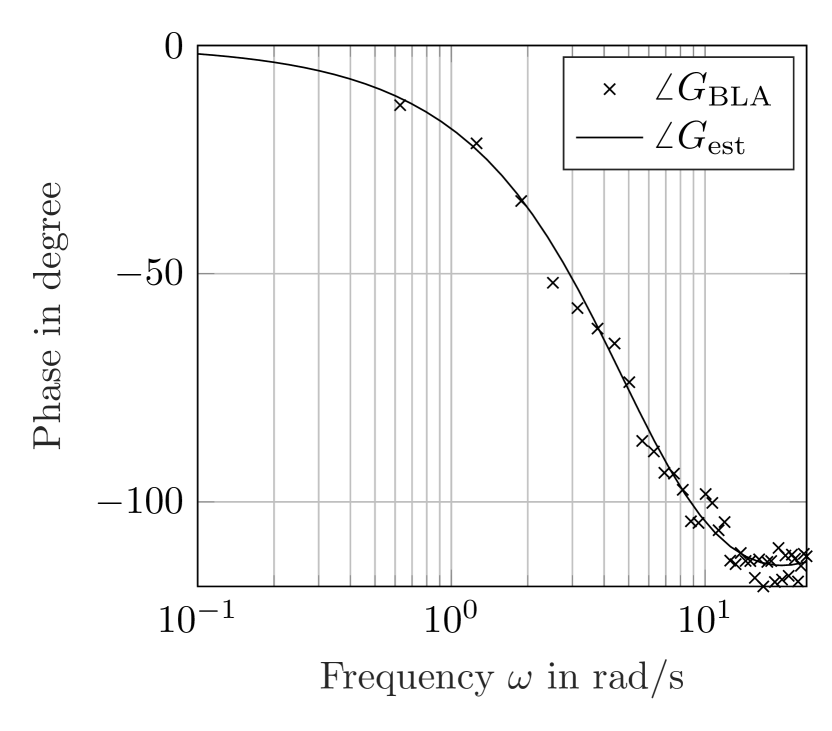
(b) phase diagram

Figure 6: The figure displays the amplitude diagram (left) and phase diagram (right) of the system response in the frequency domain. Crosses represent the measured data obtained through system identification in frequency domain, while the solid line represents the fitted transfer function. The nonlinearity system is denoted by circles in the amplitude diagram.

Additionally, we estimate the closed-loop system gradient $\mathcal{G}^{\circ}\left(\omega_{\text{ff}},\omega_{\text{fb}},\zeta\right)$ using (16):

$$\mathcal{G}^{\circ}\left(\omega_{\text{ff}},\omega_{\text{fb}},\zeta\right)=\left(\mathrm{I}-\mathcal{G}\frac{\partial\pi_{\text{fb}}\left(\omega_{\text{fb}};\zeta^{\circ}\right)}{\partial\zeta^{\circ}}\right)^{\dagger}\mathcal{G}.$$

5.1.3 Network and Input Structure

As mentioned in Section 4, each iteration necessitates the cyber-physical system to track a distinct reference trajectory. This means that the parameterized network $\pi$, particularly the feedforward network $\pi_{\text{ff}}$, must be able to adapt to reference trajectories of different lengths. The situation in the case of the beam experiment is illustrated in Figure 7. The policy network $\pi_{\text{ff}}$ takes in a horizon of $h_{1}$ steps in the past and $h_{2}$ steps in the future to produce the input $u_{k,\text{ff}}$ at time $k$ (see Figure 7(a)), while $\pi_{\text{fb}}$ takes only $h_{1}$ steps in the past to produce $u_{k,{\text{fb}}}$(see Figure 7(b)). In instances where the horizon surpasses the range of the reference trajectory, we employ a zero-padding strategy to compensate for the absent elements.

(a) structure of input, output and network for $\pi_{\text{ff}}$

(b) structure of input, output and network for $\pi_{\text{fb}}$

Figure 7: The figure illustrates the input, output, and network structures of both $\pi_{\text{ff}}$ and $\pi_{\text{fb}}$. The feedforward network $\pi_{\text{ff}}$, which is a fully connected network, utilizes the reference trajectory at time $k$, as well as the reference trajectories for the horizons of $h_{1}$ and $h_{2}$ before and after this time, as its input. The output is the corresponding feedforward input $u_{k,\text{ff}}$ at time $k$. On the other hand, the feedback network $\pi_{\text{fb}}$, a linear network, employs the trajectory difference for a horizon of $h_{1}$ units leading up to time $k$ as its input. The output is the respective feedback input $u_{k,\text{fb}}$ at time $k$. The trajectory difference is defined as the difference between the output trajectory and the reference trajectory.

5.1.4 Experiments

In this section, we employ two strategies to parameterize the feedforward network $\pi_{\text{ff}}$. One is a linear network, denoted as $\pi^{1}_{\text{ff}}$. The other is a nonlinear network, represented by $\pi^{2}_{\text{ff}}$, which is a fully-connected network with a single hidden layer. The ReLU function is used as the activation function for the hidden layer, and no activation function is applied to the output layer. We consistently use a linear feedback network $\pi_{\text{fb}}$, and considering the causality of the system, the feedback network only contains the historical information, implying that $h_{2}=0$.

The overview of different experiments is presented in Table 3. In a noise-free environment, trajectory tracking can be viewed as a purely feedforward control task. Therefore, in Experiments $1$-$4$, we employ only the feedforward network $\pi_{\text{ff}}$ and adjust the parameter $\epsilon$, allowing Algorithm 2 to transition between gradient descent ($\epsilon\rightarrow\infty$) and the quasi-Newton method. Through these experiments, we explore the convergence rates of different networks and investigate the influence of different algorithms on convergence as well as their robustness to the selection of hyper-parameters. Subsequently, we intentionally introduce noise $n_{\text{d}}$ to the inputs of the system (see Figure 2(a)), rendering the pure feedforward network ineffective for the task at hand (see Experiment $5$). Experiment $6$ demonstrates the ability of the combined feedforward and feedback control ($\pi_{\text{ff}}$ and $\pi_{\text{fb}}$) to resist noise in online learning.

exp.	model(s)	$h_{1}$	$h_{2}$	hidden	noise	$\epsilon$	$\alpha$	$\eta$	average loss
				neurons
$1$	$\pi^{1}_{\text{ff}}$	$100$	$100$	-	no	$+\infty$	-	$0.1$	$6.90\text{\times}{10}^{-3}$
$2$	$\pi^{1}_{\text{ff}}$	$100$	$100$	-	no	$1.0$	$0.1$	$15.0$	$6.30\text{\times}{10}^{-3}$
$3$	$\pi^{2}_{\text{ff}}$	$100$	$100$	$40$	no	$+\infty$	-	$0.1$	$8.27\text{\times}{10}^{-4}$
$4$	$\pi^{2}_{\text{ff}}$	$100$	$100$	$40$	no	$1.0$	$0.1$	$15.0$	$3.19\text{\times}{10}^{-4}$
$5$	$\pi^{2}_{\text{ff}}$	$100$	$100$	$40$	yes	$1.0$	$0.1$	$15.0$	$1.10\text{\times}{10}^{-3}$
$6$	$\pi^{2}_{\text{ff}}$	$100$	$100$	$40$	yes	$1.0$	$0.1$	$15.0$	$4.65\text{\times}{10}^{-4}$
	$\pi_{\text{fb}}$	$25$	-	-

Table 3: Overview of parameters, network configurations, and experimental results.

In each experiment, we train the parameterized networks for $1000$ iterations. The average loss $\delta_{t}$ is given by

$$\delta_{t}=\frac{1}{t}\sum_{k=1}^{t}l\left(y_{k};y_{\text{ref},k}\right),~{}t=1,\dots,T.$$

The convergence results of Experiments $1$ and $3$ are illustrated in Figure 8(a), while the results of Experiments $2$ and $4$ are shown in Figure 8(b). We note that, limited by the complexity of the model, the convergence results of nonlinear models are significantly better than those of linear models, regardless of whether the gradient descent algorithm or the quasi-Newton method is used. At the same time, we also notice that, under the premise of using nonlinear models, the convergence results of the quasi-Newton method are superior to those of the gradient descent algorithm. We believe that this is due to Term $2$ in (17), which is used to capture the local curvature of the loss functions, and the absence of Term $1$ in (17), leading to a lack of constraint on the changes in the outputs of $\pi_{\text{ff}}$ and $\pi_{\text{fb}}$. In our experiments, such a constraint is important for our online learning tasks, ensuring that the outputs between iterations do not change drastically, thereby preventing oscillations. Moreover, the quasi-Newton method demonstrates greater robustness in the adjustment of hyperparameters, such as the step size $\eta$, which requires additional fine-tuning for the gradient descent algorithm.

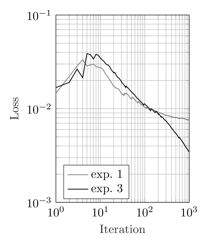
(a) results of exp. 1 and 3

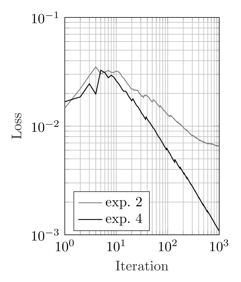
(b) results of exp. 2 and 4

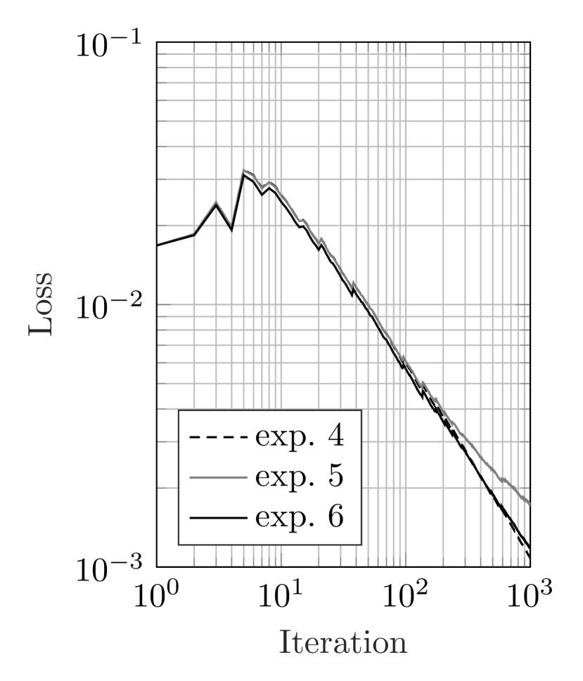
(c) results of exp. 4, 5 and 6

Figure 8: This figure depicts the convergence results $\delta_{t},~{}t=1,\dots,1000$ of different experiments.

In Experiment $5$, we artificially introduce noise $n_{\text{d}}$ to render the purely feedforward control ineffective in trajectory tracking and introduce a feedback controller in Experiment $6$ to reject noise, with the convergence results shown in Figure 8(c). The introduction of the feedback controller successfully rejects the process noise.

Additionally, we evaluate the performance of all the obtained parameterized networks trained in different experiments on a newly generated test data set previously unseen by our algorithms (see the average loss in Table 3), in order to investigate the generalization capability of the networks. Although we only utilize a linear static gradient estimate $\mathcal{G}$ (which, unsurprisingly, is a very poor estimate), the algorithms still perform well using either gradient descent method or quasi-Newton method, reflecting its strong robustness to modeling errors.

Lastly, we select a trajectory from the test data set to demonstrate the tracking performance of the models obtained in Experiments $2$ and $4$. The upper subfigure of Figure 9 shows the positions of the beam controlled by the linear and nonlinear models at different selected moments. The lower subfigure illustrates the tracking error of the beam tip in the $y$-direction as controlled by the different models.

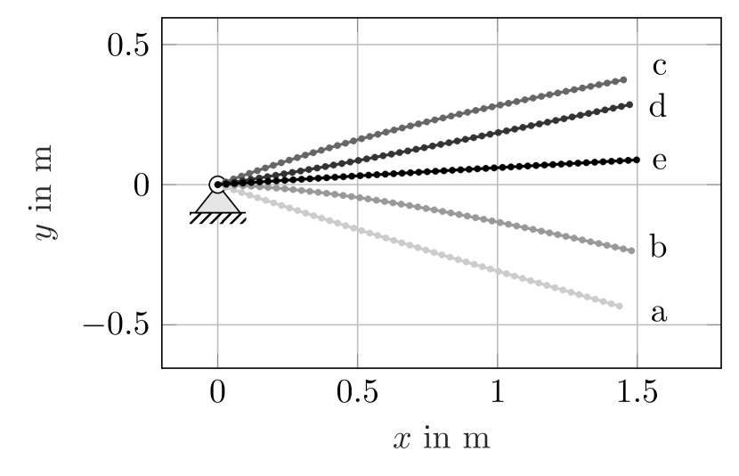
(a) motion of the beam in exp. $2$

(b) motion of the beam in exp. $4$

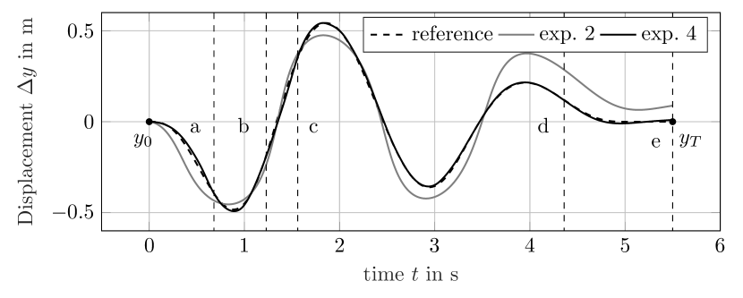
(c) motion of the tip in $y$-direction

Figure 9: This figure shows the overall motion of the beam (upper) and the motion of the tip in the $y$-direction (lower) when the models obtained in Experiments $2$ and $4$ track the reference trajectory from test data set. The motion starts from a standstill and proceeds in the order of a-b-c-d-e, with the corresponding moments marked with the same labels in the lower subfigure.

5.2 Four-Legged Robot

In this simulation, we adopt the ant model (Schulman et al., 2018) frequently used to demonstrate reinforcement learning algorithms to evaluate the effectiveness of our algorithms. The ant model is a quadruped robot with four legs symmetrically distributed around the torso, each connected by two hinged joints, providing two degrees of rotational freedom per leg and eight degrees in total for the ant. In our simulation environment, we have chosen Isaac Gym (Makoviychuk et al., 2021) for its ability to support large-scale parallel simulations, which enables us to rapidly estimate system gradients using a stochastic finite difference method. It is important to emphasize that the traditional reinforcement learning task on this model focuses on enabling the ant to move forward as quickly as possible. However, in our experiment, our aim is to enable the ant to track any reference trajectory of the center of the mass of the torso. It should be noted that in this experiment, we do not artificially introduce system noise, thus the trajectory tracking task can be considered a purely feedforward control task. Therefore, we only employ a feedforward model $\pi_{\text{ff}}$, which implies that $\pi_{\text{fb}}=0$.

We recognize that the learning of the motion of the ant, without any prior knowledge, is a challenging task. Compared to the numerical examples mentioned in Section 5.1, the learning of the motion present the following differences and difficulties: First, due to the contacts and interactions between the ant and the environment, the motion of the ant is non-smooth, and accordingly, its gradients are discontinuous (though still assumed to be bounded). Second, the states of the ant are not fully observable. In fact, in this experiment only the information about the torso is assumed to be measurable and observable, including its positions, orientations, and corresponding velocities and angular velocities. This means that changes in control inputs do not necessarily cause changes in the outputs. For instance, when one of the legs is not in contact with the ground, the positional change of this leg caused by input variation will not affect the posture of the torso. Third, walking, as a periodic behavior, should follow specific gaits and frequencies. Training a network model from scratch may lead to the ant exhibiting anomalous behaviors.

To overcome the challenges mentioned above, we make the following adjustments to the networks in this experiment:

1. We input the entire reference trajectory for $k=0$ to $k=T_{\text{sim}}$ into the model and predict the entire control sequence for $k=0$ to $k=T_{\text{sim}}$.

2. We fix the duration of the trajectory, but we can still adapt the networks to varying trajectory lengths through appropriate preprocessing.

3. We use a pre-trained linear model to provide prior knowledge of ant motion patterns.

5.2.1 Reference Trajectory Distribution

In this experiment, we can only measure and observe the information about the torso, which includes the position of the torso, its orientation represented by a quaternion, and the translational and angular velocities of the torso. The ant moves on a rough and infinitely flat plane, therefore the reference trajectories contain only three components: the planar position of the torso, i.e., the $x$ and $y$ coordinates, and the yaw, which is the rotation of the torso around the $z$-axis.

Figure 10 displays the distribution of the reference trajectories used for tracking. We take one of the sampled trajectories as an example to illustrate the general rules for generating reference trajectories. The trajectories are generated over a time duration of $T_{\text{sim}}=\qty{4}{}$. The starting point $p_{0}$ is fixed at the point $\left[0,0\right]^{\text{T}}$ in the $x$-$y$ plane at time $t_{0}=\qty{0}{}$, and the initial velocity $v_{0}$ is also fixed at $\qty{1}{\per}$ directed along the positive $x$-axis. Next, we uniformly generate the point $p_{1}$ within a disk centered around $p_{0}$ with radii of $\qty{2}{}$ and $\qty{2.5}{}$, and an angular span of $\pm\qty{60}{}$ centered around $v_{0}$ (see the red dashed disk in the left subfigure). The velocity $v_{1}$ at $p_{1}$ is also set to $\qty{1}{\per}$, in the direction of the line from $p_{0}$ to $p_{1}$. The time $t_{1}$ for generating $p_{1}$ is uniformly within a range of $\pm\qty{0.3}{}$ centered around $t=\qty{2}{}$ (see the shadow areas in the right subfigures). Based on the point $p_{1}$, the point $p_{2}$ and its corresponding velocity $v_{2}$ are generated in the same manner, with the time point $t_{2}=\qty{4}{}$ being fixed for $p_{2}$. The acceleration at each point is set to zero. Finally, we connect these three points using a trajectory that minimizes jerk. We note that the duration of all trajectories is fixed. However, since the time duration $T_{\text{sim}}$ is sufficiently long to accommodate multiple gaits, trajectories with varying durations can still be accommodated simply by periodically reapplying $\pi_{\text{ff}}$ and $\pi_{\text{fb}}$.

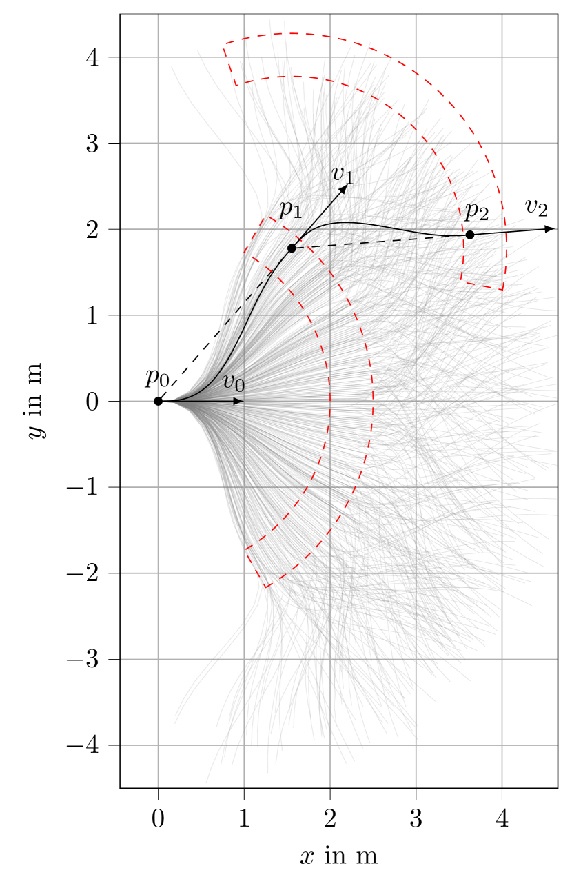
(a) distribution of reference trajectories

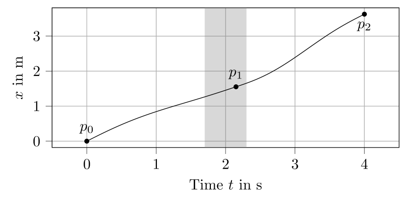
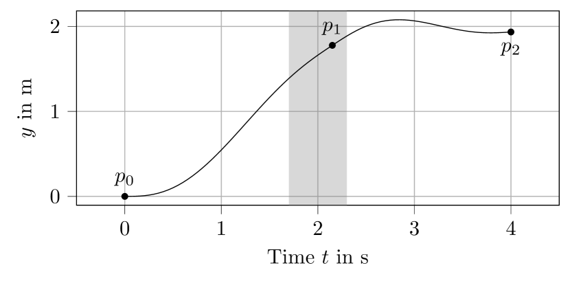
(b) trajectory of $x$

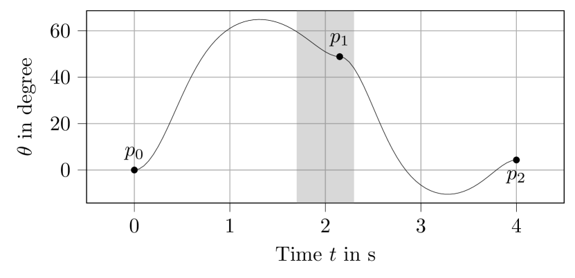
(c) trajectory of $y$

(d) trajectory of yaw

Figure 10: The left subfigure shows the area generated by $500$ randomly sampled reference trajectories used for tracking (depicted as grey lines), along with an example reference trajectory to illustrate the rules for generating trajectories (shown as a black line). The red dashed disks represent the distribution range for the position of the next point in the $x$-$y$ plane, assuming the previous point is determined. The radial gap of the disk is $\qty{0.5}{}$, with an angular span $\pm$ $\qty{60}{}$ centered around the tangent direction at the previous point. The right subfigure illustrates the temporal evolution of the example reference trajectory, showing its $x$, $y$, and yaw components. The time points for generating points $p_{0}$ and $p_{2}$ are fixed. The grey areas in the right subfigures represent the time range for point $p_{1}$, which is centered around $t=\qty{2}{}$ with a permissible deviation of $\pm\qty{0.3}{}$.

5.2.2 Gradient Estimation

In the context of the ant model, which is a system characterized by contacts and non-smooth motion, employing system identification methods as described in Section 5.1 is not applicable. Fortunately, the powerful parallel simulation capability of the Isaac Gym environment allows us to easily estimate the system gradient $\mathcal{G}\left(u_{t}\right)$ using a stochastic finite difference method. At each iteration, we run $n_{\text{env}}$ (here $n_{\text{env}}=2000$) identical environments in parallel in addition to the nominal environment. The nominal input $u_{t},~{}t=1,\dots,T$, is fed into the nominal environment, yielding the corresponding nominal output $y_{t}$. For the remaining parallel environments, normally distributed noise $n_{\text{d}}$ with a mean of zero and a variance of one is added to the nominal input $u_{t}$ (see Figure 2(a)), denoted as $\widetilde{u}_{t,i},~{}i=1,\dots,n_{\text{env}}$, resulting in the respective outputs $\widetilde{y}_{t,i}$. Finally, we estimate the system gradient $\mathcal{G}\left(u_{t}\right)$ using least squares:

$$\mathcal{G}\left(u_{t}\right)^{\text{T}}=\begin{bmatrix}\left(\widetilde{u}_{t,1}-u_{t}\right)^{\text{T}}\\ \left(\widetilde{u}_{t,2}-u_{t}\right)^{\text{T}}\\ \vdots\\ \left(\widetilde{u}_{t,n_{\text{env}}}-u_{t}\right)^{\text{T}}\end{bmatrix}^{\dagger}\begin{bmatrix}\left(\widetilde{y}_{t,1}-y_{t}\right)^{\text{T}}\\ \left(\widetilde{y}_{t,2}-y_{t}\right)^{\text{T}}\\ \vdots\\ \left(\widetilde{y}_{t,n_{\text{env}}}-y_{t}\right)^{\text{T}}\end{bmatrix},$$

where we stack all inputs and outputs by columns respectively.

5.2.3 Neural Network with Pre-Trained Motion Patterns

In order to enable online learning with the ant model, we parameterize our networks as follows:

$$\pi_{\text{ff}}\left(\omega_{\text{ff}};\zeta\right)=U\phi\left(\omega_{\text{ff}};V^{\text{T}}\zeta\right),~{}\pi_{\text{fb}}=0,$$

where the matrices $U\in\mathbb{R}^{mq\times n_{\sigma}}$ and $V\in\mathbb{R}^{nq\times n_{\sigma}}$ represent linear transformation to a lower dimensional latent space and $\phi:\mathbb{R}^{n_{\omega_{\text{ff}}}}\times\mathbb{R}^{n_{\sigma}}\rightarrow\mathbb{R}^{mq}$ is a neural network comprising one hidden layer. The matrices $U$ and $V$ are obtained through a pretraining process based on $45$ trajectories. Further details about the pretraining process and obtaining the matrices $U$ and $V$ are included in Appendix C.

5.2.4 Experiments

In this experiment, we use a fully connected network with only one hidden layer containing $20$ neurons. The hidden layer employs the ReLU activation function, while the output layer does not have an activation function. We employ different methods to train the network, and the parameters are shown in Table 4.

exp.	model	$n_{\sigma}$	hidden	$\epsilon$	$\alpha$	$\eta$
			neurons
$1$	$\pi_{\text{ff}}$	$90$	45	$+\infty$	-	diminishing
$2$	$\pi_{\text{ff}}$	$45$	20	$0.1$	$0.5$	$0.1$

Table 4: Parameters for training the ant model.

The two experiments were conducted with over $1500$ and $3500$ iterations, respectively, and their convergence results are shown in Figure 11. We note that the loss of both algorithms eventually converges to the same level with the same rate. However, it is important to emphasize that to ensure the convergence of the gradient descent method, its step size $\eta_{t}$ must be carefully designed. In contrast, the quasi-Newton method demonstrates much stronger robustness to the step size selection. Finally, through this experiment, we demonstrate that in such complex cyber-physical system, even with a poor gradient estimate, our algorithms still ensure convergence and exhibit high robustness to modeling errors. It is important to emphasize that, unlike RL, which optimizes a feedback policy to enable the ant to move forward as fast as possible, our algorithms learn a feedforward model $\pi_{\text{ff}}$ that allows the ant to track any reference trajectories sampled from the distribution $p_{y_{\text{ref}}}$, thereby truly enabling it to learn the skill of walking. Additionally, our algorithms are capable of continuously improving the tracking performance of the feedforward network through online learning during deployment.

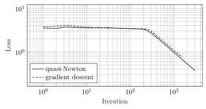
Figure 11: The figure shows the convergence results of the gradient descent and quasi-Newton method. The gray line represents the average loss of the gradient descent method, and the black line indicates the average loss of the quasi-Newton method.

We select one of the trajectories in Figure 12 to demonstrate the tracking performance of the neural network trained by the quasi-Newton method. The left subfigure shows the tracking performance in the three-dimensional space, where the reference trajectory is set at a fixed height of $\qty{0.5}{}$. The right subfigures separately demonstrate the tracking performance of the model for the $x$, $y$, and yaw components of the trajectory.

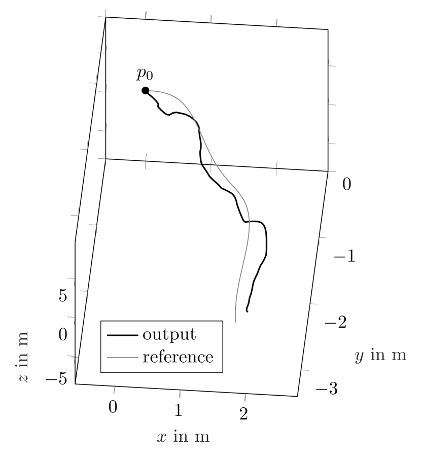
(a) trajectory in the three-dimensional space

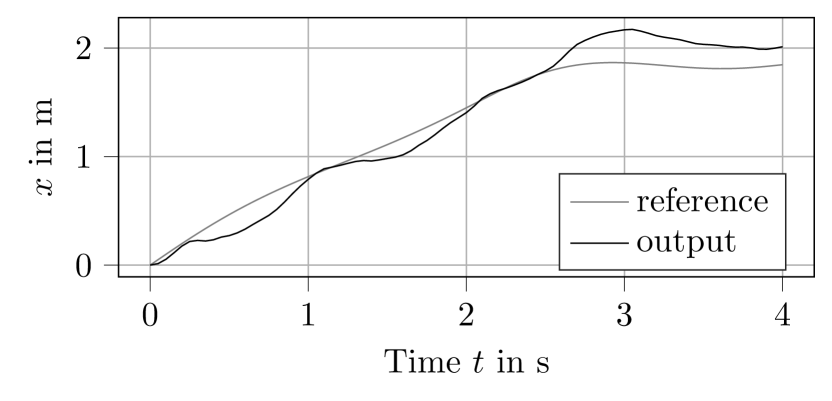
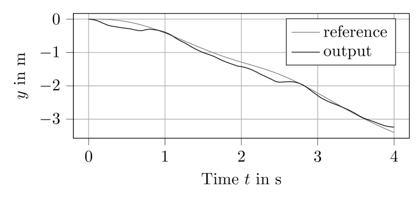
(b) trajectory of $x$

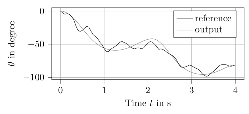
(c) trajectory of $y$

(d) trajectory of yaw

Figure 12: The figure shows the tracking performance of the network trained by the quasi-Newton method on a single reference trajectory. The left subfigure illustrates the tracking effect of the network in the three-dimensional space, where the $z$-value of the reference trajectory is chosen to be $\qty{0.5}{}$. The right subfigures separately show the tracking performance of the network for the $x$, $y$, and yaw components.

5.3 Table Tennis Robot

In this experiment, we evaluate the effectiveness of our algorithms in a real-world cyber-physical system, which is a robotic arm actuated by pneumatic artificial muscles (PAMs) as shown in Figure 13. This robotic arm is designed for playing table tennis. The PAMs offer a high power-to-weight ratio enabling rapid movements, but also introduce substantial nonlinearities to the system, making the precise control of this robotic arm particularly challenging.

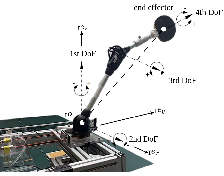
Figure 13: The figure shows the structure of the robot arm. It has four rotational joints, and each joint is actuated by a pair of PAMs. The unit vectors ${}_{\mathrm{I}}e_{x}$, ${}_{\mathrm{I}}e_{y}$ and ${}_{\mathrm{I}}e_{z}$ together form the global coordinate system $\left\{\mathrm{I}\right\}$ with ${}_{\mathrm{I}}o$ as the origin. For simplicity we consider only DoF $1-3$, whereas DoF $4$ is controlled with a PID controller.

The robot has four rotational degrees of freedom (DoF), each powered by a pair of PAMs. For more information about this robot, please refer to Ma et al. (2022); Büchler et al. (2022, 2016). In this experiment, we only consider learning the controller for the first three degrees of freedom, as the last degree of freedom can be accurately controlled with a PID controller.

5.3.1 Reference Trajectory Distribution

In this experiment, the distribution of the reference trajectories is tailored to the specific task of playing table tennis. First, we fix the initial posture $p_{\text{ini}}$ of the robot, and then determine the interception point $p_{\text{int}}$ based on the incoming trajectory of the table tennis ball. The robot moves from the initial posture to the interception point and then returns to the initial posture. Each trajectory is planned within a polar coordinate system using a minimum jerk trajectory that connects $p_{\text{ini}}$ and $p_{\text{int}}$. For more detailed information and the specific form of the trajectory, please refer to Ma et al. (2022, 2023).

5.3.2 Gradient Estimation

Each degree of freedom is highly coupled with the others. However, for estimating the gradient, we disregard the coupling between each degree of freedom, thereby decomposing the system into three independent subsystems. This allows for the gradient estimation for each degree of freedom separately. The input for each degree of freedom consists of the pressure values from two artificial muscles, and the output is the angle of the degree of freedom. We further reduce the number of inputs by setting a baseline pressure and controlling the pressure difference between the two artificial muscles and the baseline. Subsequently, we use the method described in Section 5.1 to identify the transfer function for each simplified degree of freedom in the frequency domain and use this to estimate a static gradient $\mathcal{G}^{i},~{}i=1,2,3$ for each degree of freedom. Please refer to Ma et al. (2022) for details on the system identification and the construction of the approximate gradient.

5.3.3 Network and Input Structure

We construct three structurally identical linear network models, $\pi_{\text{ff}}^{i},~{}i=1,2,3$ as in Section 5.1. Although the coupling between different degrees of freedom is ignored for the gradient estimation, the coupling is accounted for by the online learning. Therefore, we use the reference trajectories of all three degrees of freedom as inputs to each linear model. The method for generating the inputs is also described in Section 5.1, where $h=100$.

5.3.4 Experiments

The reference trajectories are derived from past interceptions of table tennis balls, and we use $30$ reference trajectories for training. In our online learning approach, we randomly sample a reference trajectory without replacement. Once every reference trajectory has been executed we start a new epoch, where we again sample one trajectory at random without replacement.

The convergence of the online learning is shown in Figure 14, with each epoch distinguished by vertical dashed lines. It is observed that the average tracking errors of all three linear models converge with the same rate. This suggests that through the training, the linear models are capable of capturing the coupling effects between different degrees of freedom. It is important to emphasize that even with a rough estimate of the gradient, our algorithm achieves rapid convergence and maintains stability in a highly complex nonlinear system. This not only underlines the robustness of our algorithm against modeling errors but also provides empirical evidence of its performance on real-world systems.

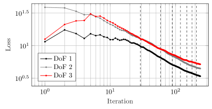
Figure 14: This figure illustrates the average tracking error for each degree of freedom. Each independent linear model is trained by a pseudo-online learning approach, wherein each trajectory is randomly sampled without replacement in every epoch. A total of $30$ reference trajectories are available for training in each epoch. Each epoch is distinguished in the figure by vertical dashed lines.

We select one trajectory from the last training epoch to demonstrate the tracking performance of the linear models. In Figure 15, the left subfigure shows the tracking performance of the tip of the robot in three-dimensional space. The right subfigures separately show the tracking performance for each degree of freedom.

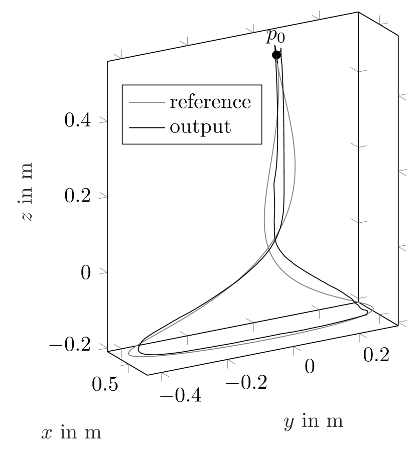
(a) trajectory in three-dimensional space

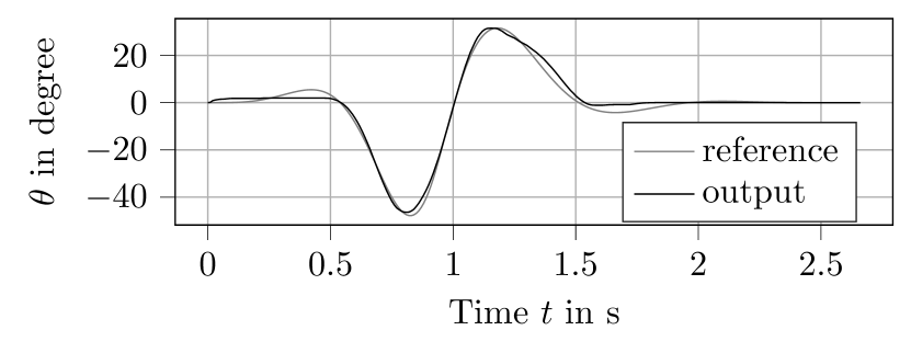
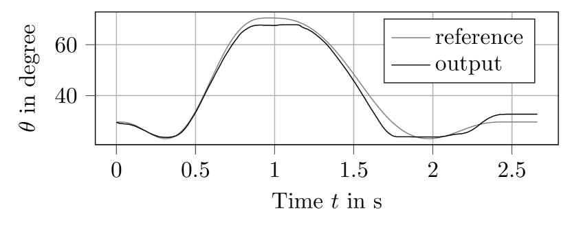
(b) trajectory of DoF $1$

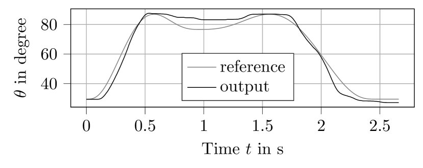
(c) trajectory of DoF $2$

(d) trajectory of DoF $3$

Figure 15: The figure demonstrates the tracking performance of a reference trajectory from the last training epoch. The left subfigure shows the tracking performance of the tip of the robot in three-dimensional space. The right subfigures separately show the tracking performance for each degree of freedom.

6 Conclusions

In this article, we propose a novel gradient-based online learning framework derived from a trust-region approach, operating under the assumptions that the loss functions are smooth but not required to be convex. Thanks to gradient information that is incorporated within the algorithm, we obtain a sample efficient online learning approach that is applicable to cyber-physical and robotic systems. The framework presented in this article includes a stochastic optimization algorithm, various designs for neural networks and input structures for feedforward and feedback control scenarios. We have not only theoretically proven the convergence of the algorithm without relying on convexity, but also evaluated the effectiveness of our proposed framework through a wide range of examples, including numerical experiments, simulation experiments, and real-world implementations. These experiments highlight fast convergence of our algorithms and robustness against modeling errors. Furthermore, they provide empirical evidence that this algorithm can be deployed in real-world applications in the future.

Acknowledgments

Hao Ma and Michael Muehlebach thank the German Research Foundation, the Branco Weiss Fellowship, administered by ETH Zurich, and the Center for Learning Systems for the funding support.

A Derivation of Trust-Region Approach

In this appendix, we will present in detail the necessary intermediate steps used to derive the results in Section 3. We start from the local approximation of the function $M\left(v,\omega\right)$

$$\begin{split}M\left(v,\omega\right)=&\underbrace{f\left(\omega\right)+\nabla f\left(\omega\right)^{\text{T}}\left(v-\omega\right)+\frac{1}{2}\left(v-\omega\right)^{\text{T}}\nabla^{2}f\left(\omega\right)\left(v-\omega\right)}_{\text{second order Taylor expansion}}\\ &+\underbrace{\frac{\alpha}{2}\left|\pi\left(v\right)-\pi\left(\omega\right)\right|^{2}}_{\text{Term 1}}+\underbrace{\frac{\epsilon}{2}\left|v-\omega\right|^{2}}_{\text{Term 2}}.\end{split}$$ (17)

To obtain (9), it is important to note that, as specified in (17), calculating the gradient and Hessian matrix of the loss function $f$ is essential, which can be expressed as follows:

$$\begin{split}\nabla f\left(\omega\right)&=\frac{\partial y^{\text{T}}}{\partial\omega}\nabla_{y}l\left(y;\zeta\right),\\ \nabla^{2}f\left(\omega\right)&=\frac{\partial^{2}y^{\text{T}}}{\partial\omega^{2}}\nabla_{y}l\left(y;\zeta\right)+\frac{\partial y^{\text{T}}}{\partial\omega}\nabla^{2}_{y}l\left(y;\zeta\right)\frac{\partial y}{\partial\omega},\end{split}$$ (18)

where we introduce

$$\frac{\partial y}{\partial\omega}\approx\mathcal{L}=\left(\mathrm{I}-\mathcal{G}\left(u\right)\frac{\partial\pi\left(\omega,y;\zeta\right)}{\partial y}\right)^{\dagger}\mathcal{G}\left(u\right)\frac{\partial\pi\left(\omega,y;\zeta\right)}{\partial\omega},$$

and assume

$$\frac{\partial^{2}y}{\partial\omega^{2}}\approx 0.$$

Then, (17) can be formulated as follows:

$$\begin{split}M\left(v,\omega\right)=&f\left(\omega\right)+\left(v-\omega\right)^{\text{T}}\mathcal{L}^{\text{T}}\nabla_{y}l\left(y;\zeta\right)+\frac{1}{2}\left(v-\omega\right)^{\text{T}}\mathcal{L}^{\text{T}}\nabla^{2}_{y}l\left(y;\zeta\right)\mathcal{L}\left(v-\omega\right)\\ &+\frac{\alpha}{2}\left|\pi\left(v\right)-\pi\left(\omega\right)\right|^{2}+\frac{\epsilon}{2}\left|v-\omega\right|^{2}.\end{split}$$

We further perform a Taylor expansion of $\pi\left(v\right)$ around $\pi\left(\omega\right)$, that is,

$$\pi\left(v\right)=\pi\left(\omega\right)+\left.\frac{\partial\pi\left(\omega\right)}{\partial\omega}\right|_{\omega}\left(v-\omega\right)+\text{HOT},$$

where HOT denotes the remaining higher order term. This yields (9).

To obtain (10), we calculate the expectation of $M\left(v,\omega\right)$ as follows:

$$\begin{split}\mathbb{E}_{\zeta}\left[M(v,\omega)|\omega\right]=&\underbrace{\int f\left(\omega;\xi\right)p_{\zeta}\left(\xi\right)\text{d}\xi}_{F\left(\omega\right)}+\left(v-\omega\right)^{\text{T}}\int\mathcal{L}\left(\xi\right)^{\text{T}}\nabla_{y}l\left(y;\xi\right)p_{\zeta}\left(\xi\right)\text{d}\xi\\ &+\frac{1}{2}\left(v-\omega\right)^{\text{T}}\underbrace{\int\mathcal{L}\left(\xi\right)^{\text{T}}\nabla^{2}_{y}l\left(y;\xi\right)\mathcal{L}\left(\xi\right)p_{\zeta}\left(\xi\right)\text{d}\xi}_{\epsilon{\Sigma}_{1}}\left(v-\omega\right)\\ &+\frac{\alpha}{2}\left(v-\omega\right)^{\text{T}}\underbrace{\int\nabla_{\omega}\pi\left(\omega;\xi\right)\nabla_{\omega}\pi\left(\omega;\xi\right)^{\text{T}}~{}p_{\zeta}\left(\xi\right)\text{d}\xi}_{\epsilon{\Sigma}_{2}}\left(v-\omega\right)\\ &+\frac{\epsilon}{2}\left(v-\omega\right)^{\text{T}}\left(v-\omega\right).\end{split}$$ (19)

B Proof of Theorem 2.1

In this appendix we will prove Theorem 2.1. First of all, we show that Assumption 2.4 implies the following inequality:

$$\left|\mathbb{E}_{\zeta}\left[\left.\mathcal{F}\left(\omega_{t};\zeta\right)\right|\omega_{t}\right]-\mathbb{E}_{\zeta}\left[\left.\nabla f\left(\omega_{t};\zeta\right)\right|\omega_{t}\right]\right|^{2}_{A_{t-1}^{-1}}\leq\kappa^{2}\left|\mathbb{E}_{\zeta}\left[\left.\nabla f\left(\omega;\zeta\right)\right|\omega\right]\right|^{2}_{A_{t-1}^{-1}}.$$

Lemma B.1

Let

$$\lambda_{\mathrm{max}}\left(P\right)\left|y-x\right|^{2}\leq\kappa^{2}\lambda_{\mathrm{min}}\left(P\right)\left|x\right|^{2}$$ (20)

be satisfied for all $x,y\in\mathbb{R}^{n}$, $\kappa\in\left[0,1\right)$, and for a positive definite matrix $P\in\mathbb{R}^{n\times n}$, then the following inequality holds

$$\left|y-x\right|^{2}_{P}\leq\kappa^{2}\left|x\right|^{2}_{P}.$$

Proof  We prove Lemma B.1 via a contradiction argument. We first assume that there exists $x,y\in\mathbb{R}^{n}$ such that (20) is satisfied and the following inequality holds

$$\left|y-x\right|^{2}_{P}>\kappa^{2}\left|x\right|^{2}_{P},$$

which implies that

$$\lambda_{\mathrm{max}}\left(P\right)\left|y-x\right|^{2}\geq\left|y-x\right|^{2}_{P}>\kappa^{2}\left|x\right|^{2}_{P}\geq\kappa^{2}\lambda_{\mathrm{min}}\left(P\right)\left|x\right|^{2}.$$

Then we have

$$\lambda_{\mathrm{max}}\left(P\right)\left|y-x\right|^{2}>\kappa^{2}\lambda_{\mathrm{min}}\left(P\right)\left|x\right|^{2},$$

which contradicts (20). This concludes the proof of Lemma B.1.  
We note that a key difficulty in the proof of Theorem 2.1 is that the stochastic gradients and the matrices $A_{t}^{-1}$ are dependent random variables. We will therefore in a first step, represent the inverse of the matrix $A_{t}$ using $A_{t-1}^{-1}$ in order to decouple the dependency.

Proposition B.1

Consider the sequence of pseudo-Hessian matrices $A_{t}$ obtained according to Algorithm 2. Then, the following relationship between $A_{t-1}^{-1}$ and $A_{t}^{-1}$ holds for all $t\geq 2$,

$$A_{t}^{-1}=\frac{t}{t-1}A^{-1}_{t-1}-\frac{t}{\left(t-1\right)^{2}}R_{t}\left(\mathrm{I}+\frac{1}{t-1}R_{t}\right)^{-1}A_{t-1}^{-1},$$

where

$$R_{t}:=A^{-1}_{t-1}\left(\frac{\mathcal{L}_{t}^{\mathrm{T}}\nabla^{2}_{y}l\left(y_{t};\zeta_{t}\right)\mathcal{L}_{t}}{\epsilon}+\frac{\alpha\nabla_{\omega}\pi\left(\omega_{t},y_{t};\zeta_{t}\right)\nabla_{\omega}\pi\left(\omega_{t},y_{t};\zeta_{t}\right)^{\mathrm{T}}}{\epsilon}+\mathrm{I}\right),~{}\zeta_{t}\stackrel{{\scriptstyle\mathrm{i.i.d.}}}{{\sim}}p_{\zeta}.$$

Proof  We start with the definition of $A_{t}$,

$$\begin{split}A_{t}&=\frac{t-1}{t}A_{t-1}+\frac{1}{t}\frac{\mathcal{L}_{t}^{\mathrm{T}}\nabla^{2}_{y}l\left(y_{t};\zeta_{t}\right)\mathcal{L}_{t}+\alpha\nabla_{\omega}\pi\left(\omega_{t},y_{t};\zeta_{t}\right)\nabla_{\omega}\pi\left(\omega_{t},y_{t};\zeta_{t}\right)^{\mathrm{T}}}{\epsilon}+\frac{1}{t}\text{I}\\ &=\frac{t-1}{t}A_{t-1}\left(\text{I}+\frac{1}{t-1}R_{t}\right),~{}\forall t\geq 2.\end{split}$$

In addition, we notice that the matrix $A_{t}$ is always positive definite due to the addition of the identity matrix $\mathrm{I}$. Therefore, we can calculate the inverse of $A_{t}$ as follows:

$$\begin{split}A_{t}^{-1}=&\frac{t}{t-1}\left(\mathrm{I}+\frac{1}{t-1}R_{t}\right)^{-1}A_{t-1}^{-1}\\ =&\frac{t}{t-1}\left[\mathrm{I}-\frac{1}{t-1}R_{t}\left(\mathrm{I}+\frac{1}{t-1}R_{t}\right)^{-1}\right]A_{t-1}^{-1}\\ =&\frac{t}{t-1}A^{-1}_{t-1}-\frac{t}{\left(t-1\right)^{2}}R_{t}\left(\mathrm{I}+\frac{1}{t-1}R_{t}\right)^{-1}A_{t-1}^{-1},~{}\forall t\geq 2.\end{split}$$

 
We now prove Theorem 2.1.

Proof  We start by analyzing the decrease of $F\left(\omega_{t+1}\right)$ conditioned on $\omega_{1:T}$, where we substitute the iterative scheme in Algorithm 2. We obtain the following result:

$$\begin{split}&\mathbb{E}_{\zeta_{t}}\left[\left.F(\omega_{t+1})-F(\omega_{t})\right|\omega_{1:t}\right]=\mathbb{E}_{\zeta_{t}}\left[\left.F\left(\omega_{t}-\eta_{t}A_{t}^{-1}\mathcal{F}\left(\omega_{t};\zeta_{t}\right)\right)-F(\omega_{t})\right|\omega_{1:t}\right]\\ \leq&\mathbb{E}_{\zeta_{t}}\left[\left.-\eta_{t}\nabla F(\omega_{t})^{\text{T}}A_{t}^{-1}\mathcal{F}\left(\omega_{t};\zeta_{t}\right)+\frac{L\eta_{t}^{2}}{2}\left|A_{t}^{-1}\mathcal{F}\left(\omega_{t};\zeta_{t}\right)\right|^{2}\right|\omega_{1:t}\right]\\ \leq&-\mathbb{E}_{\zeta_{t}}\left[\left.\eta_{t}\nabla F(\omega_{t})^{\text{T}}A_{t}^{-1}\mathcal{F}\left(\omega_{t};\zeta_{t}\right)\right|\omega_{1:t}\right]+\frac{LH^{2}\eta_{t}^{2}}{2},\end{split}$$ (21)

where the first inequality arises from the $L$-smoothness of $F\left(\omega\right)$, while the second inequality stems from Assumption 2.2 the fact that $\nicefrac{{1}}{{\lambda}}\leq\left\|A^{-1}_{t}\right\|\leq 1$:

$$\mathbb{E}_{\zeta_{t}}\left[\left.\left|A_{t}^{-1}\mathcal{F}\left(\omega_{t};\zeta_{t}\right)\right|^{2}\right|\omega_{1:t}\right]\leq\left\|A_{t}^{-1}\right\|^{2}\mathbb{E}_{\zeta_{t}}\left[\left.\left|\mathcal{F}\left(\omega_{t};\zeta_{t}\right)\right|^{2}\right|\omega_{1:t}\right]\leq H^{2},$$

where $\left\|\cdot\right\|$ denotes the spectral norm of a matrix.

Next we rearrange (21) and get the following expression:

$$\mathbb{E}_{\zeta_{t}}\left[\left.\eta_{t}\nabla F(\omega_{t})^{\text{T}}A_{t}^{-1}\mathcal{F}\left(\omega_{t};\zeta_{t}\right)\right|\omega_{1:t}\right]\leq\mathbb{E}_{\zeta_{t}}\left[\left.F\left(\omega_{t}\right)-F\left(\omega_{t+1}\right)\right|\omega_{1:t}\right]+\frac{LH^{2}\eta_{t}^{2}}{2}.$$ (22)

By substituting the result of Proposition B.1 into the term on the left-hand side, we have the following result:

$$\begin{split}&\eta_{t}\nabla F(\omega_{t})^{\text{T}}A_{t}^{-1}\mathcal{F}\left(\omega_{t};\zeta_{t}\right)\\ =&\eta_{t}\nabla F(\omega_{t})^{\text{T}}\left(\frac{t}{t-1}A^{-1}_{t-1}-\frac{t}{(t-1)^{2}}R_{t}\left(\mathrm{I}+\frac{1}{t-1}R_{t}\right)^{-1}A_{t-1}^{-1}\right)\mathcal{F}\left(\omega_{t};\zeta_{t}\right)\\ =&\frac{\eta_{t}t}{t-1}\nabla F(\omega_{t})^{\text{T}}A_{t-1}^{-1}\left(\nabla f\left(\omega_{t};\zeta_{t}\right)-\nabla f\left(\omega_{t};\zeta_{t}\right)+\mathcal{F}\left(\omega_{t};\zeta_{t}\right)\right)\\ &-\frac{\eta_{t}t}{(t-1)^{2}}\nabla F(\omega_{t})^{\text{T}}R_{t}\left(\mathrm{I}+\frac{1}{t-1}R_{t}\right)^{-1}A_{t-1}^{-1}\mathcal{F}\left(\omega_{t};\zeta_{t}\right)\\ \geq&\frac{\eta_{t}t}{t-1}\nabla F(\omega_{t})^{\text{T}}A_{t-1}^{-1}\left(\nabla f\left(\omega_{t};\zeta_{t}\right)-\nabla f\left(\omega_{t};\zeta_{t}\right)+\mathcal{F}\left(\omega_{t};\zeta_{t}\right)\right)\\ &-\frac{\eta_{t}\lambda}{t-1}\left|\nabla F\left(\omega_{t}\right)\right|\left|\mathcal{F}\left(\omega_{t};\zeta_{t}\right)\right|,~{}\forall t\geq 2.\end{split}$$ (23)

The last inequality is obtained due to the following facts:

$$\left\|R_{t}\right\|\leq\left\|A^{-1}_{t-1}\right\|\left\|\frac{\mathcal{L}_{t}^{\text{T}}\nabla^{2}_{y}l\left(y_{t};\zeta_{t}\right)\mathcal{L}_{t}}{\epsilon}+\frac{\alpha\pi_{\omega}\left(\omega_{t},y_{t};\zeta_{t}\right)\pi_{\omega}\left(\omega_{t},y_{t};\zeta_{t}\right)^{\text{T}}}{\epsilon}+\text{I}\right\|\leq\lambda,$$

and

$$\begin{split}&\left\|\left(\mathrm{I}+\frac{1}{t-1}R_{t}\right)^{-1}A_{t-1}^{-1}\right\|\\ =&\left\|\left(A_{t-1}+\frac{1}{t-1}\left(\frac{\mathcal{L}_{t}^{\text{T}}\nabla^{2}_{y}l\left(y_{t};\zeta_{t}\right)\mathcal{L}_{t}}{\epsilon}+\frac{\alpha\pi_{\omega}\left(\omega_{t},y_{t};\zeta_{t}\right)\pi_{\omega}\left(\omega_{t},y_{t};\zeta_{t}\right)^{\text{T}}}{\epsilon}+\text{I}\right)\right)^{-1}\right\|\leq\frac{t-1}{t}.\end{split}$$

For $t=1$ we have

$$\begin{split}&\eta_{1}\nabla F(\omega_{1})^{\text{T}}\left(\frac{\mathcal{L}_{1}^{\text{T}}\nabla^{2}_{y}l\left(y_{1};\zeta_{1}\right)\mathcal{L}_{1}}{\epsilon}+\frac{\alpha\pi_{\omega}\left(\omega_{1},y_{1};\zeta_{1}\right)\pi_{\omega}\left(\omega_{1},y_{1};\zeta_{1}\right)^{\text{T}}}{\epsilon}+\text{I}\right)^{-1}\mathcal{F}\left(\omega_{1};\zeta_{1}\right)\\ =&\eta_{1}\nabla F(\omega_{1})^{\text{T}}\left(\text{I}-R_{1}\left(\text{I}+R_{1}\right)^{-1}\right)\mathcal{F}\left(\omega_{1};\zeta_{1}\right)\\ \geq&\eta_{1}\nabla F(\omega_{1})^{\text{T}}\left(\nabla f\left(\omega_{1};\zeta_{1}\right)-\nabla f\left(\omega_{1};\zeta_{1}\right)+\mathcal{F}\left(\omega_{1};\zeta_{1}\right)\right)-\eta_{1}\lambda\left|\nabla F\left(\omega_{1}\right)\right|\left|\mathcal{F}\left(\omega_{1};\zeta_{1}\right)\right|,\end{split}$$ (24)

where

$$R_{1}:=\frac{\mathcal{L}_{1}^{\mathrm{T}}\nabla^{2}_{y}l\left(y_{1};\zeta_{1}\right)\mathcal{L}_{1}}{\epsilon}+\frac{\alpha\nabla_{\omega}\pi\left(\omega_{1},y_{1};\zeta_{1}\right)\nabla_{\omega}\pi\left(\omega_{1},y_{1};\zeta_{1}\right)^{\mathrm{T}}}{\epsilon}+\mathrm{I},~{}\zeta_{1}\stackrel{{\scriptstyle\mathrm{i.i.d.}}}{{\sim}}p_{\zeta}.$$

We now substitute the result of (23) into (22) and rearrange the terms. We evaluate conditional expectations on both sides as follows:

$$\begin{split}&\frac{\eta_{t}t}{t-1}\mathbb{E}_{\zeta_{t}}\left[\left.\nabla F(\omega_{t})^{\text{T}}A_{t-1}^{-1}\left(\nabla f\left(\omega_{t};\zeta_{t}\right)-\nabla f\left(\omega_{t};\zeta_{t}\right)+\mathcal{F}\left(\omega_{t};\zeta_{t}\right)\right)\right|\omega_{1:t}\right]\\ =&\frac{\eta_{t}t}{t-1}\nabla F(\omega_{t})^{\text{T}}A_{t-1}^{-1}\nabla F\left(\omega_{t}\right)-\frac{\eta_{t}t}{t-1}\mathbb{E}_{\zeta_{t}}\left[\left.\nabla F(\omega_{t})^{\text{T}}A_{t-1}^{-1}\left(\nabla f\left(\omega_{t};\zeta_{t}\right)-\mathcal{F}\left(\omega_{t};\zeta_{t}\right)\right)\right|{\omega_{1:t}}\right].\end{split}$$

Then, we apply the Peter-Paul inequality and Lemma B.1 to the second term, and get the following result:

$$\mathbb{E}_{\zeta_{t}}\left[\left.\nabla F(\omega_{t})^{\text{T}}A_{t-1}^{-1}\left(\nabla f\left(\omega_{t};\zeta_{t}\right)-\mathcal{F}\left(\omega_{t};\zeta_{t}\right)\right)\right|{\omega_{1:t}}\right]$$

$$= \nabla F(\omega_{t})^{\text{T}}A_{t-1}^{-1}\left(\nabla F\left(\omega_{t}\right)-\mathbb{E}_{\zeta_{t}}\left[\left.\mathcal{F}\left(\omega_{t};\zeta_{t}\right)\right|\omega_{1:t}\right]\right)$$

$$\leq \frac{\kappa}{2}\nabla F(\omega_{t})^{\text{T}}A_{t-1}^{-1}\nabla F\left(\omega_{t}\right)+\frac{1}{2\kappa}\left|\nabla F\left(\omega_{t}\right)-\mathbb{E}_{\zeta_{t}}\left[\left.\mathcal{F}\left(\omega_{t};\zeta_{t}\right)\right|\omega_{1:t}\right]\right|^{2}_{A_{t-1}^{-1}}$$

$$\leq \frac{\kappa}{2}\left|\nabla F(\omega_{t})\right|^{2}_{A_{t-1}^{-1}}+\frac{\kappa}{2}\left|\nabla F(\omega_{t})\right|^{2}_{A_{t-1}^{-1}}$$

$$= \kappa\left|\nabla F(\omega_{t})\right|^{2}_{A_{t-1}^{-1}}.$$

Meanwhile, we have

$$\mathbb{E}_{\zeta_{t}}\left[\left.\left|\nabla F\left(\omega_{t}\right)\right|\left|\mathcal{F}\left(\omega_{t};\zeta_{t}\right)\right|\right|\omega_{1:t}\right]\leq\mathbb{E}_{\zeta_{t}}\left[\left.\left|\nabla F\left(\omega_{t}\right)\right|\right|\omega_{1:t}\right]\mathbb{E}_{\zeta_{t}}\left[\left.\left|\mathcal{F}\left(\omega_{t};\zeta_{t}\right)\right|\right|\omega_{1:t}\right]\leq H^{2},$$

as a result of Jensen’s inequality. At last, we have

$$\frac{\eta_{t}t}{t-1}\mathbb{E}_{\zeta_{t}}\left[\left.\nabla F(\omega_{t})^{\text{T}}A_{t-1}^{-1}\mathcal{F}\left(\omega_{t};\zeta_{t}\right)\right|\omega_{1:t}\right]\geq\frac{\eta_{t}t\left(1-\kappa\right)}{t-1}\left|\nabla F\left(\omega_{t}\right)\right|^{2}_{A_{t-1}^{-1}}-\frac{\eta_{t}H^{2}\lambda}{t-1}.$$

For $t=1$ we have

$$\eta_{1}\mathbb{E}_{\zeta_{1}}\left[\left.\nabla F(\omega_{1})^{\text{T}}\mathcal{F}\left(\omega_{1};\zeta_{1}\right)\right|\omega_{1}\right]\geq\eta_{1}\left(1-\kappa\right)\left|\nabla F(\omega_{1})\right|^{2}-\eta_{1}H^{2}\lambda.$$

Further, we get the following result by considering the expectation over all random variables on both sides in (22):

$$\begin{split}\left(1-\kappa\right)\frac{\eta_{t}t}{t-1}\mathbb{E}_{\zeta_{1:T}}\left[\left|\nabla F(\omega_{t})\right|^{2}_{A^{-1}_{t-1}}\right]\leq&\mathbb{E}_{\zeta_{1:T}}\left[F\left(\omega_{t}\right)\right]-\mathbb{E}_{\zeta_{1:T}}\left[F\left(\omega_{t+1}\right)\right]\\ &+\frac{LH^{2}\eta_{t}^{2}}{2}+\frac{\eta_{t}H^{2}\lambda}{t-1},~{}\forall t\geq 2.\end{split}$$ (25)

We note that

$$\mathbb{E}_{\zeta_{1:T}}\left[\left|\nabla F(\omega_{t})\right|^{2}_{A_{t}^{-1}}\right]\leq\frac{t}{t-1}\mathbb{E}_{\zeta_{1:T}}\left[\left|\nabla F(\omega_{t})\right|^{2}_{A_{t-1}^{-1}}\right],~{}\forall t\geq 2,$$

and

$$\mathbb{E}_{\zeta_{1:T}}\left[\left|\nabla F(\omega_{1})\right|^{2}_{A_{1}^{-1}}\right]\leq\mathbb{E}_{\zeta_{1:T}}\left[\left|\nabla F(\omega_{1})\right|^{2}\right].$$

In the following, we exploit the fact that the step size is constant, that is, $\eta_{t}=\eta$ for all $t\geq 1$. As a consequence, (25) can be rewritten as follows:

$$\begin{split}\left(1-\kappa\right)\mathbb{E}_{\zeta_{1:T}}\left[\left|\nabla F(\omega_{t})\right|^{2}_{A_{t}^{-1}}\right]\leq&\frac{\mathbb{E}_{\zeta_{1:T}}\left[F(\omega_{t})\right]-\mathbb{E}_{\zeta_{1:T}}\left[F(\omega_{t+1})\right]}{\eta}+\frac{LH^{2}\eta}{2}+\frac{H^{2}\lambda}{t-1},~{}\forall t\geq 2.\end{split}$$

By summing up the above equation and including the case $t=1$ we get the following result:

$$\left(1-\kappa\right)\sum_{t=1}^{T}\mathbb{E}_{\zeta_{1:T}}\left[\left|\nabla F(\omega_{t})\right|^{2}_{A_{t}^{-1}}\right]\leq\frac{F\left(\omega_{1}\right)-F\left(\omega^{\star}\right)}{\eta}+\frac{TLH^{2}\eta}{2}+H^{2}\lambda\sum_{t=1}^{T}a_{t},~{}\forall t\geq 1,$$

where we notice that $F(\omega^{\star})\leq\mathbb{E}_{\zeta_{1:T}}\left[F(\omega_{T+1})\right]$ always holds since $\omega^{\star}$ denotes the global minimum, and $a_{t}$ is defined as $a_{1}=1$, $a_{t}=\nicefrac{{1}}{{t-1}}$ for $t\geq 2$. The above equation can be further simplified due to the fact that $F\left(\omega^{\star}\right)\geq 0$:

$$\left(1-\kappa\right)\sum_{t=1}^{T}\mathbb{E}_{\zeta_{1:T}}\left[\left|\nabla F(\omega_{t})\right|^{2}_{A_{t}^{-1}}\right]\leq\frac{F\left(\omega_{1}\right)}{\eta}+\frac{TLH^{2}\eta}{2}+H^{2}\lambda\sum_{t=1}^{T}a_{t},~{}\forall t\geq 1.$$ (26)

The sum over $a_{t}$ is bounded as follows:

$$\begin{split}\sum_{t=1}^{T}a_{t}&\leq\int_{2}^{T}\frac{1}{t-1}\mathrm{d}t+2\\ &=\ln{\left(T-1\right)}+2\\ &\leq\ln{T}+2,~{}\forall T\geq 1.\end{split}$$ (27)

We substitute (27) into (26) and calculate its average value as follows:

$$\left(1-\kappa\right)\frac{1}{T}\sum_{t=1}^{T}\mathbb{E}_{\zeta_{1:T}}\left[\left|\nabla F(\omega_{t})\right|^{2}_{A_{t}^{-1}}\right]\leq\frac{F\left(\omega_{1}\right)}{\eta T}+\frac{LH^{2}\eta}{2}+\frac{\lambda H^{2}\left(\ln{T}+2\right)}{T}.$$ (28)

We set the first two terms on the right-hand side to be equal by choosing the step size appropriately,

$$\frac{F\left(\omega_{1}\right)}{\eta T}=\frac{LH^{2}\eta}{2}\Leftrightarrow\eta=\sqrt{\frac{2F\left(\omega_{1}\right)}{LH^{2}T}}.$$

This yields the following result:

$$\frac{1-\kappa}{T}\sum_{t=1}^{T}\mathbb{E}_{\zeta_{1:T}}\left[\left|\nabla F(\omega_{t})\right|^{2}_{A_{t}^{-1}}\right]\leq\sqrt{\frac{2LH^{2}F\left(\omega_{1}\right)}{T}}+\frac{\lambda H^{2}\left(\ln{T}+2\right)}{T},$$

which is dominated by the first term on the right-hand side of the inequality for large $T$. It also implies that the average expected gradient will converge to zero at a rate of $\mathcal{O}\left(\nicefrac{{1}}{{\sqrt{T}}}\right)$.  

C Pretraining Process

In this appendix, we will briefly explain the pretraining process that is used in Section 5.2. The matrices $U$ and $V$ are obtained through the singular value decomposition of the matrix $R$:

$$R=U\mathrm{diag}\left(\sigma\right)V^{\mathrm{T}},$$

where the matrix $R$ is derived by solving the following ridge regression:

$$\min_{R\in\mathbb{R}^{mq\times nq}}~{}\sum_{i=1}^{n_{\text{ILC}}}\left\|u_{\text{ref},i}-Ry_{\text{ref},i}\right\|^{2}_{\text{F}}+\frac{\rho}{2}\left\|R\right\|^{2}_{\text{F}},$$

where $\rho$ is a positive constant, and $\left\|\cdot\right\|_{\text{F}}$ denotes the Frobenius norm. The ideal input $u_{\text{ref}}$ represents the input required for accurately tracking a given reference trajectory $y_{\text{ref}}$. The ideal input is unknown, and we therefore employ iterative learning control (ILC) to approximate it (Ma et al., 2022; Hofer et al., 2019; Zughaibi et al., 2021; Mueller et al., 2012; Schoellig et al., 2012; Zughaibi et al., 2024). The variable $n_{\text{ILC}}$ denotes the number of pre-trained trajectories using ILC. In this experiment, we sample $50$ reference trajectories and get their corresponding ideal inputs using ILC, and each reference trajectory takes $200$ to $300$ iterations to obtain the ideal inputs. We then use $45$ trajectories ($$90$\%$) along with their ideal inputs to perform ridge regression. Figure 16 displays the distribution composed of all $50$ reference trajectories used for pre-training in the left subfigure, whereas the right subfigure showcases the final training result of ILC for one reference trajectory as an example. The right subfigures illustrate the tracking performance of the corresponding $x$, $y$, and yaw components of this trajectory. We note that the tracking of the $x$ and $y$ components by the ILC is very effective; however, due to the presence of collisions, the tracking of the yaw component is slightly less accurate. Nevertheless, we consider this as a sufficiently good ideal input for tracking the given reference trajectory, which is able to capture the motion patterns.

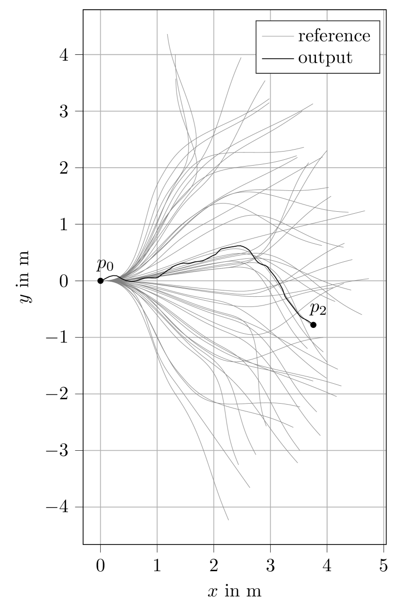
(a) distribution of trajectories for ILC

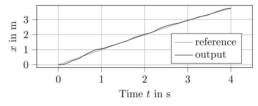
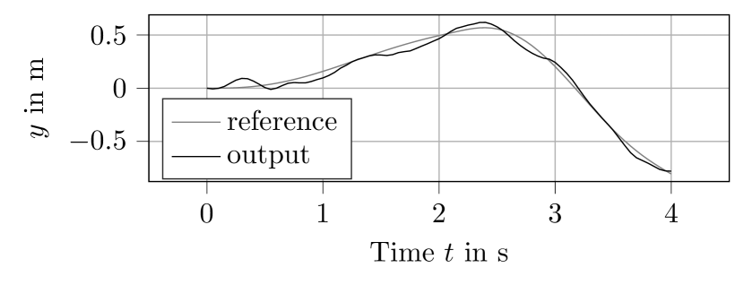
(b) trajectory of $x$

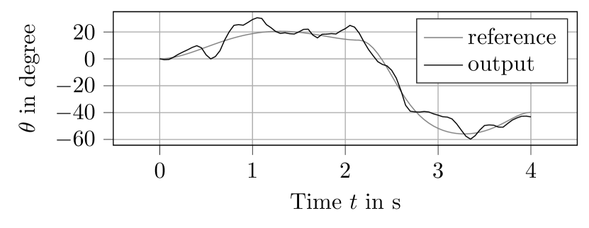
(c) trajectory of $y$

(d) trajectory of yaw

Figure 16: The left subfigure shows the distribution of $50$ randomly sampled reference trajectories used for pre-training (represented by gray lines), and illustrates the tracking performance of ILC with one of these trajectories (depicted as a black line). The right subfigures demonstrate the tracking performance of the ILC for the particular trajectory in the $x$, $y$, and yaw components.

References

- Abernethy et al. (2009) Jacob Abernethy, Elad Hazan, and Alexander Rakhlin. Competing in the Dark: An Efficient Algorithm for Bandit Linear Optimization. In Proceedings of Annual Conference on Learning Theory, pages 1–11, 2009.
- Agarwal et al. (2017a) Naman Agarwal, Brian Bullins, and Elad Hazan. Second-Order Stochastic Optimization for Machine Learning in Linear Time. Journal of Machine Learning Research, 18(1):4148–4187, 2017a.
- Agarwal et al. (2017b) Naman Agarwal, Brian Bullins, and Elad Hazan. Second-Order Stochastic Optimization for Machine Learning in Linear Time. Journal of Machine Learning Research, 18(1):4148–4187, 2017b.
- Amirouche (2007) Farid Amirouche. Fundamentals of Multibody Dynamics: Theory and Applications. Springer Science & Business Media, 2007.
- Auer et al. (2002) Peter Auer, Nicoè Cesa-Bianchi, and Paul Fischer. Finite-Time Analysis of the Multiarmed Bandit Problem. Machine Learning, 47(2-3):235–256, 2002.
- Bernstein et al. (2019) Andrey Bernstein, Emiliano Dall’Anese, and Andrea Simonetto. Online Primal-Dual Methods With Measurement Feedback for Time-Varying Convex Optimization. IEEE Transactions on Signal Processing, 67(8):1978–1991, 2019.
- Bertsekas (2015) Dimitri Bertsekas. Convex Optimization Algorithms. Athena Scientific, 2015.
- Bottou (2010) Léon Bottou. Large-Scale Machine Learning with Stochastic Gradient Descent. In Proceedings of International Conference on Computational Statistics, pages 177–186, 2010.
- Bottou et al. (2018) Léon Bottou, Frank E Curtis, and Jorge Nocedal. Optimization Methods for Large-Scale Machine Learning. SIAM Review, 60(2):223–311, 2018.
- Boyd and Vandenberghe (2004) Stephen P. Boyd and Lieven Vandenberghe. Convex Optimization. Cambridge University Press, 2004.
- Broyden (1970) Charles G. Broyden. The Convergence of a Class of Double-rank Minimization Algorithms 1. General Considerations. IMA Journal of Applied Mathematics, 6(1):76–90, 1970.
- Bubeck (2011) Sébastien Bubeck. Introduction to Online Optimization. Lecture Notes, 2(1):1–86, 2011.
- Bubeck (2012) Sébastien Bubeck. Regret Analysis of Stochastic and Nonstochastic Multi-armed Bandit Problems. Foundations and Trends in Machine Learning, 5(1):1–122, 2012.
- Büchler et al. (2016) Dieter Büchler, Heiko Ott, and Jan Peters. A Lightweight Robotic Arm with Pneumatic Muscles for Robot Learning. In Proceedings of IEEE International Conference on Robotics and Automation, pages 4086–4092, 2016.
- Büchler et al. (2022) Dieter Büchler, Simon Guist, Roberto Calandra, Vincent Berenz, Bernhard Schölkopf, and Jan Peters. Learning to Play Table Tennis From Scratch Using Muscular Robots. IEEE Transactions on Robotics, 38(6):3850–3860, 2022.
- Byrd et al. (2011) Richard H. Byrd, Gillian M. Chin, Will Neveitt, and Jorge Nocedal. On the Use of Stochastic Hessian Information in Optimization Methods for Machine Learning. SIAM Journal on Optimization, 21(3):977–995, 2011.
- Campi and Weyer (2002) Marco C. Campi and Erik Weyer. Finite Sample Properties of System Identification Methods. IEEE Transactions on Automatic Control, 47(8):1329–1334, 2002.
- Carè et al. (2018) Algo Carè, Balázs Cs. Csáji, Marco C. Campi, and Erik Weyer. Finite-Sample System Identification: An Overview and a New Correlation Method. IEEE Control Systems Letters, 2(1):61–66, 2018.
- Cesa-Bianchi and Lugosi (2006) Nicolo Cesa-Bianchi and Gabor Lugosi. Prediction, Learning, and Games. Cambridge University Press, 2006.
- Cesa-Bianchi et al. (2005) Nicolò Cesa-Bianchi, Alex Conconi, and Claudio Gentile. A Second-Order Perceptron Algorithm. SIAM Journal on Computing, 34(3):640–668, 2005.
- Cheng and Chen (2014) Hongtai Cheng and Heping Chen. Online Parameter Optimization in Robotic Force Controlled Assembly Processes. In Proceedings of IEEE International Conference on Robotics and Automation, pages 3465–3470, 2014.
- Colombino et al. (2020) Marcello Colombino, Emiliano Dall’Anese, and Andrey Bernstein. Online Optimization as a Feedback Controller: Stability and Tracking. IEEE Transactions on Control of Network Systems, 7(1):422–432, 2020.
- Crammer et al. (2006) Koby Crammer, Ofer Dekel, Joseph Keshet, Shai Shalev-Shwartz, and Yoram Singer. Online Passive-Aggressive Algorithms. Journal of Machine Learning Research, 7(19):551–585, 2006.
- Crammer et al. (2013) Koby Crammer, Alex Kulesza, and Mark Dredze. Adaptive Regularization of Weight Vectors. Machine learning, 91(1):155–187, 2013.
- Crespi and Ijspeert (2008) Alessandro Crespi and Auke J. Ijspeert. Online Optimization of Swimming and Crawling in an Amphibious Snake Robot. IEEE Transactions on Robotics, 24(1):75–87, 2008.
- Defazio et al. (2014) Aaron Defazio, Francis Bach, and Simon Lacoste-Julien. SAGA: A Fast Incremental Gradient Method With Support for Non-Strongly Convex Composite Objectives. In Proceedings of Advances in Neural Information Processing Systems, pages 1–9, 2014.
- Dekel et al. (2012) Ofer Dekel, Ran Gilad-Bachrach, Ohad Shamir, and Lin Xiao. Optimal Distributed Online Prediction Using Mini-Batches. Journal of Machine Learning Research, 13(1):165–202, 2012.
- Dembo et al. (1982) Ron S. Dembo, Stanley C. Eisenstat, and Trond Steihaug. Inexact Newton Methods. SIAM Journal on Numerical Analysis, 19(2):400–408, 1982.
- Dredze et al. (2008) Mark Dredze, Koby Crammer, and Fernando Pereira. Confidence-Weighted Linear Classification. In Proceedings of International Conference on Machine Learning, pages 264–271, 2008.
- Fletcher (1970) Roger Fletcher. A New Approach to Variable Metric Algorithms. The Computer Journal, 13(3):317–322, 1970.
- Freund and Schapire (1997) Yoav Freund and Robert E. Schapire. A Decision-Theoretic Generalization of On-line Learning and an Application to Boosting. Journal of Computer and System Sciences, 55(1):119–139, 1997.
- Geering (2007) Hans P. Geering. Optimal Control with Engineering Applications. Springer, 2007.
- Gentile (2000) Claudio Gentile. A New Approximate Maximal Margin Classification Algorithm. Journal of Machine Learning Research, 2(1):213–242, 2000.
- Golub and Loan (2013) Gene H. Golub and Charles F. Van Loan. Matrix Computations. JHU Press, 2013.
- Hall and Willett (2015) Eric C. Hall and Rebecca M. Willett. Online Convex Optimization in Dynamic Environments. IEEE Journal of Selected Topics in Signal Processing, 9(4):647–662, 2015.
- Hauswirth et al. (2017) Adrian Hauswirth, Alessandro Zanardi, Saverio Bolognani, Florian Dorfler, and Gabriela Hug. Online Optimization in Closed Loop on the Power Flow Manifold. In Proceedings of IEEE Manchester PowerTech, pages 1–6, 2017.
- Hazan (2022) Elad Hazan. Introduction to Oline Convex Optimization. MIT Press, 2022.
- Hazan and Kale (2010) Elad Hazan and Satyen Kale. An Optimal Algorithm for Stochastic Strongly-Convex Optimization. arXiv, 1006.2425:1–6, 2010.
- Hazan et al. (2007a) Elad Hazan, Amit Agarwal, and Satyen Kale. Logarithmic reegret algorithms for online convex optimization. Machine Learning, 69(2):169–192, 2007a.
- Hazan et al. (2007b) Elad Hazan, Alexander Rakhlin, and Peter Bartlett. Adaptive Online Gradient Descent. In Proceedings of Advances in Neural Information Processing Systems, pages 1–8, 2007b.
- Hofer et al. (2019) Matthias Hofer, Lukas Spannagl, and Raffaello D’Andrea. Iterative Learning Control for Fast and Accurate Position Tracking with an Articulated Soft Robotic Arm. In Proceedings of International Conference on Intelligent Robots and Systems, pages 6602–6607, 2019.
- Iouditski and Nesterov (2014) Anatoli Iouditski and Yuri Nesterov. Primal-Dual Subgradient Methods for Minimizing Uniformly Convex Functions. arXiv, 1401.1792:1–32, 2014.
- Johnson and Zhang (2013) Rie Johnson and Tong Zhang. Accelerating Stochastic Gradient Descent using Predictive Variance Reduction. In Proceedings of Advances in Neural Information Processing Systems, pages 1–9, 2013.
- Kolev et al. (2023) Pavel Kolev, Georg Martius, and Michael Muehlebach. Online Learning under Adversarial Nonlinear Constraints. In Proceedings of Advances in Neural Information Processing Systems, pages 53227–53238, 2023.
- LeCun et al. (1998) Yann LeCun, Leon Bottou, Genevieve B. Orr, and Klaus-Robert Müller. Efficient BackProp. Neural Networks: Tricks of the Trade, pages 9–50, 1998.
- Li and Long (1999) Yi Li and Philip Long. The Relaxed Online Maximum Margin Algorithm. Machine Learning, 46(1):361–387, 1999.
- Li (2018) Yuxi Li. Deep Reinforcement Learning: An Overview. arXiv, 1701.07274:1–85, 2018.
- Littlestone and Warmuth (1994) Nick Littlestone and Manfred K. Warmuth. The Weighted Majority Algorithm. Information and Computation, 108(2):212–261, 1994.
- Liu and Nocedal (1989) Dong C. Liu and Jorge Nocedal. On the Limited Memory BFGS Method for Large Scale optimization. Mathematical Programming, 45(1):503–528, 1989.
- Ljung (2010) Lennart Ljung. Perspectives on System Identification. Annual Reviews in Control, 34(1):1–12, 2010.
- Ma et al. (2022) Hao Ma, Dieter Büchler, Bernhard Schölkopf, and Michael Muehlebach. A Learning-based Iterative Control Framework for Controlling a Robot Arm with Pneumatic Artificial Muscles. In Proceedings of Robotics: Science and Systems, pages 1–10, 2022.
- Ma et al. (2023) Hao Ma, Dieter Büchler, Bernhard Schölkopf, and Michael Muehlebach. Reinforcement learning with model-based feedforward inputs for robotic table tennis. Autonomous Robots, 47(8):1387–1403, 2023.
- Makoviychuk et al. (2021) Viktor Makoviychuk, Lukasz Wawrzyniak, Yunrong Guo, Michelle Lu, Kier Storey, Miles Macklin, David Hoeller, Nikita Rudin, Arthur Allshire, Ankur Handa, and Gavriel State. Isaac Gym: High Performance GPU-Based Physics Simulation For Robot Learning. arXiv, 2108.10470:1–32, 2021.
- Martens and Grosse (2015) James Martens and Roger Grosse. Optimizing Neural Networks with Kronecker-Factored Approximate Curvature. In Proceedings of International Conference on Machine Learning, pages 2408–2417, 2015.
- Martínez (1994) José Mario Martínez. Local Minimizers of Quadratic Functions on Euclidean Balls and Spheres. SIAM Journal on Optimization, 4(1):159–176, 1994.
- Mokhtari and Ribeiro (2014) Aryan Mokhtari and Alejandro Ribeiro. RES: Regularized Stochastic BFGS Algorithm. IEEE Transactions on Signal Processing, 62(23):6089–6104, 2014.
- Muehlebach (2023) Michael Muehlebach. Adaptive Decision-Making with Constraints and Dependent Losses: Performance Guarantees and Applications to Online and Nonlinear Identification. In Proceedings of IFAC World Congress, pages 5107–5114, 2023.
- Mueller et al. (2012) Fabian L. Mueller, Angela P. Schoellig, and Raffaello D’Andrea. Iterative Learning of Feed-Forward Corrections for High-Performance Tracking. In Proceedings of International Conference on Intelligent Robots and Systems, pages 3276–3281, 2012.
- Nesterov and Spokoiny (2017) Yurii Nesterov and Vladimir Spokoiny. Random Gradient-Free Minimization of Convex Functions. Foundations of Computational Mathematics, 17(2):527–566, 2017.
- Neu (2015) Gergely Neu. Explore no more: Improved high-probability regret bounds for non-stochastic bandits. In Proceedings of Advances in Neural Information Processing Systems, pages 1–9, 2015.
- Nocedal (1980) Jorge Nocedal. Updating Quasi-Newton Matrices with Limited Storage. Mathematics of Computation, 35(151):773–782, 1980.
- Nocedal and Wright (2006) Jorge Nocedal and Stephen J. Wright. Numerical Optimization. Springer, 2006.
- Novikoff (1962) Albert B.J. Novikoff. On Convergence Proofs on Perceptrons. In Proceedings of the Symposium on the Mathematical Theory of Automata, pages 615–622, 1962.
- Piazzi and Visioli (1997) Aurelio Piazzi and Antonio Visioli. An Interval Algorithm for Minimum-Jerk Trajectory Planning of Robot Manipulators. In Proceedings of IEEE Conference on Decision and Control, pages 1924–1927, 1997.
- Pilanci and Wainwright (2017) Mert Pilanci and Martin J. Wainwright. Newton Sketch: A Near Linear-Time Optimization Algorithm with Linear-Quadratic Convergence. SIAM Journal on Optimization, 27(1):205–245, 2017.
- Pintelon and Schoukens (2012) Rik Pintelon and Johan Schoukens. System Identification: A Frequency Domain Approach. John Wiley & Sons, 2012.
- Rakhlin et al. (2012) Alexander Rakhlin, Ohad Shamir, and Karthik Sridharan. Making Gradient Descent Optimal for Strongly Convex Stochastic Optimization. arXiv, 1109.5647:1–21, 2012.
- Reddi et al. (2019) Sashank J. Reddi, Satyen Kale, and Sanjiv Kumar. On the Convergence of Adam and Beyond. arXiv, 1904.09237:1–23, 2019.
- Robbins and Monro (1951) Herbert Robbins and Sutton Monro. A Stochastic Approximation Method. The Annals of Mathematical Statistics, 22(3):400–407, 1951.
- Ruder (2017) Sebastian Ruder. An Overview of Gradient Descent Optimization Algorithms. arXiv, 1609.04747:1–14, 2017.
- Schmidt et al. (2017) Mark Schmidt, Nicolas Le Roux, and Francis Bach. Minimizing Finite Sums with the Stochastic Average Gradient. Mathematical Programming, 162(1):83–112, 2017.
- Schoellig et al. (2012) Angela P. Schoellig, Fabian L. Mueller, and Raffaello D’Andrea. Optimization-Based Iterative Learning for Precise Quadrocopter Trajectory Tracking. Autonomous Robots, 33(1):103–127, 2012.
- Schraudolph (2001) Nicol N. Schraudolph. Fast Curvature Matrix-Vector Products. In Proceedings of Artificial Neural Networks, pages 19–26, 2001.
- Schraudolph et al. (2007) Nicol N. Schraudolph, Jin Yu, and Simon Günter. A Stochastic Quasi-Newton Method for Online Convex Optimization. In Proceedings of Artificial Intelligence and Statistics, pages 436–443, 2007.
- Schulman et al. (2018) John Schulman, Philipp Moritz, Sergey Levine, Michael Jordan, and Pieter Abbeel. High-Dimensional Continuous Control Using Generalized Advantage Estimation. arXiv, 1506.02438:1–14, 2018.
- Shabana (1997) Ahmed A. Shabana. Flexible Multibody Dynamics: Review of Past and Recent Developments. Multibody System Dynamics, 1(2):189–222, 1997.
- Shalev-Shwartz (2012) Shai Shalev-Shwartz. Online Learning and Online Convex Optimization. Foundations and Trends in Machine Learning, 4(2):107–194, 2012.
- Shalev-Shwartz and Singer (2007) Shai Shalev-Shwartz and Yoram Singer. A Primal-Dual Perspective of Online Learning Algorithms. Machine Learning, 69(2):115–142, 2007.
- Sorensen (1982) Danny C. Sorensen. Newton’s Method with a Model Trust Region Modification. SIAM Journal on Numerical Analysis, 19(2):409–426, 1982.
- Sutton and Barto (2018) Richard S. Sutton and Andrew G. Barto. Reinforcement Learning: An Introduction. MIT Press, 2018.
- Tobuschat et al. (2023) Philip Tobuschat, Hao Ma, Dieter Büchler, Bernhard Schölkopf, and Michael Muehlebach. Data-Efficient Online Learning of Ball Placement in Robot Table Tennis. In Proceeding of IEEE/RSJ International Conference on Intelligent Robots and Systems, pages 567–573, 2023.
- Tsiamis and Pappas (2019) Anastasios Tsiamis and George J. Pappas. Finite Sample Analysis of Stochastic System Identification. In Proceedings of IEEE Conference on Decision and Control, pages 3648–3654, 2019.
- Wang et al. (2018) Weitian Wang, Rui Li, Zachary M. Diekel, and Yunyi Jia. Robot Action Planning by Online Optimization in Human–Robot Collaborative Tasks. International Journal of Intelligent Robotics and Applications, 2(2):161–179, 2018.
- Yuan (2015) Ya-xiang Yuan. Recent Advances in Trust Region Algorithms. Mathematical Programming, 151(1):249–281, 2015.
- Zinkevich (2003) Martin Zinkevich. Online Convex Programming and Generalized Infinitesimal Gradient Ascent. In Proceedings of International Conference on Machine Learning, pages 928–936, 2003.
- Zughaibi et al. (2021) Jasan Zughaibi, Matthias Hofer, and Raffaello D’Andrea. A Fast and Reliable Pick-and-Place Application with a Spherical Soft Robotic Arm. In Proceedings of International Conference on Soft Robotics, pages 599–606, 2021.
- Zughaibi et al. (2024) Jasan Zughaibi, Bradley J. Nelson, and Michael Muehlebach. Balancing a 3D Inverted Pendulum Using Remote Magnetic Manipulation. arXiv, 2402.06012:1–8, 2024.