Long-time Self-body Image Acquisition and its Application to the Control of Musculoskeletal Structures

Abstract

The tendon-driven musculoskeletal humanoid has many benefits that human beings have, but the modeling of its complex muscle and bone structures is difficult and conventional model-based controls cannot realize intended movements. Therefore, a learning control mechanism that acquires nonlinear relationships between joint angles, muscle tensions, and muscle lengths from the actual robot is necessary. In this study, we propose a system which runs the learning control mechanism for a long time to keep the self-body image of the musculoskeletal humanoid correct at all times. Also, we show that the musculoskeletal humanoid can conduct position control, torque control, and variable stiffness control using this self-body image. We conduct a long-time self-body image acquisition experiment lasting 3 hours, evaluate variable stiffness control using the self-body image, etc., and discuss the superiority and practicality of the self-body image acquisition of musculoskeletal structures, comprehensively.

I INTRODUCTION

The tendon-driven musculoskeletal humanoid [1, 2, 3] has many benefits that human beings have, such as multiple degrees of freedom (multi-DOFs), under-actuated structures of the spine and fingers, variable stiffness control using nonlinear elasticity and antagonism of muscles, and error correction using redundant muscles. Therefore, the humanoid is expected to move flexibly like human beings and work in an environment with physical contact. At the same time, its bone and muscle structures are complex, and there are many problems which cannot be solved by conventional model-based controls. In particular, unlike the tendon-driven robot with constant moment arm [4, 5], the muscle route modeling of the musculoskeletal humanoid is very difficult.

In order to solve these problems, various studies have been conducted. There is the method which trains the neural network of the joint-muscle mapping (JMM, the nonlinear relationship between joint angles and muscle lengths) with the actual sensor information [6], the method which trains JMM using polynomial regression and estimates the current joint angles from JMM [7], and the method which obtains the Jacobian between the position and muscle length from vision [8]. Also, we have developed an online learning method of JMM using vision [9]. By extending it, we have also developed an online learning method of the self-body image considering muscle-route changes caused by body tissue softness [10].

However, because there is a large error in the joint-muscle mapping between the actual robot and its geometric model in the early stages of learning, muscle temperatures rise rapidly due to unintended high muscle tensions, and the motors of the muscles may burn out. Also, previous studies conducted the online learning for only five minutes, and long-time online learning sometimes proceeds in an unintended direction. So, we propose a mechanism to stably conduct long-time self-body image acquisition. This mechanism includes a simple online updater of the self-body image realized by separating software elasticity and hardware elasticity, data accumulation and augmentation of the actual robot sensor information for online learning, and a safety mechanism considering muscle tension and muscle temperature.

Also, previous studies have focused on the learning of the self-body image itself, so there are few studies on control methods using it. In this study, we develop the position and torque control using the acquired self-body image. Additionally, the musculoskeletal humanoid can conduct mechanical variable stiffness control, using its redundant muscles and the nonlinear elastic element of each muscle. Until now, although model-based variable stiffness control systems such as [11] have been developed, these control systems can be used only when the moment arm and nonlinear elasticity of muscles are modelized completely. Therefore, we propose an estimation of mechanical operational stiffness using the self-body image, and its control which enables the change of the operational stiffness as intended. These proposed methods will extend the range of application of musculoskeletal humanoids.

This study is important for not only the tendon-driven musculoskeletal humanoid, but also for the musculoskeletal hand, such as the ACT Hand [12], the tensegrity robot [13], soft robotics [14], etc.

In the following sections, first, we will state the overview of the musculoskeletal structure. Then, we will explain the detailed method of long-time self-body image acquisition and control systems using it, while comparing with previous studies. Finally, we will conduct several experiments of the proposed methods, and state the conclusion.

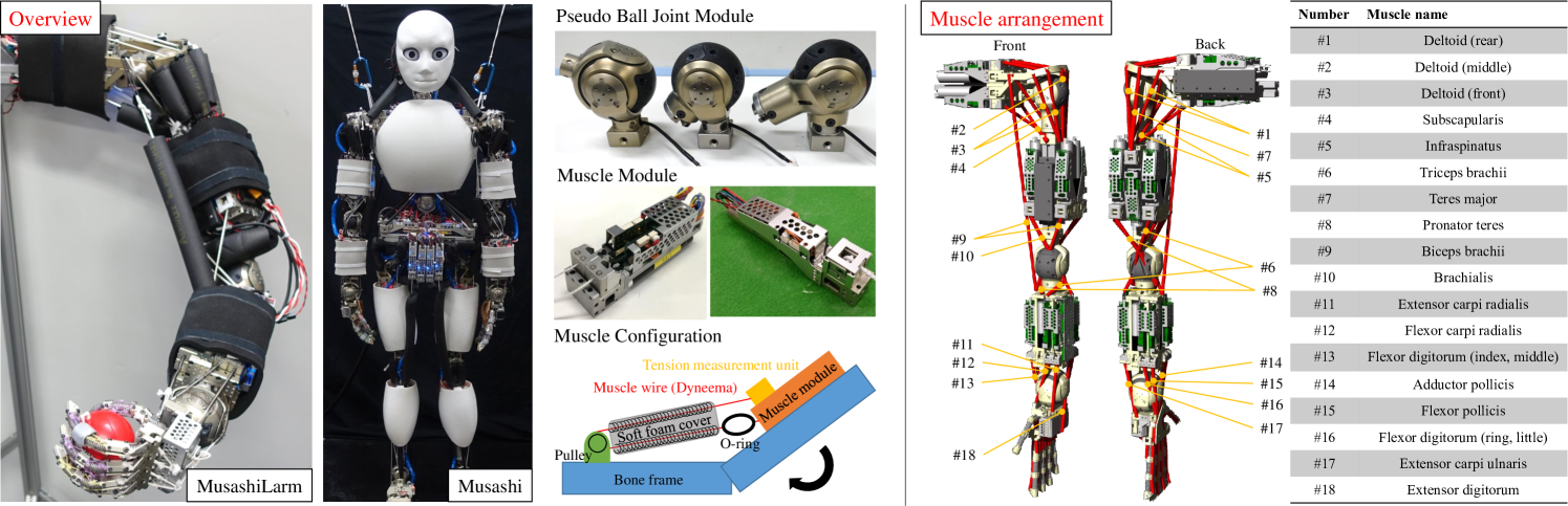
Figure 1: Overview of newly developed MusashiLarm and Musashi used in this study [15].

II Musculoskeletal Humanoid

In this study, we use MusashiLarm and Musashi [15] (Fig. 1) developed as a musculoskeletal research platform to succeed Kengoro [3].

II-A Joint Structure

MusashiLarm has 3 DOFs of the shoulder, 2 DOFs of the elbow and radioulnar joint, 2 DOFs of the wrist joint, and the fingers have flexible and robust under-actuated structures made of machined springs. Each joint is constructed by a pseudo ball joint module which can measure joint angles directly using the included potentiometers. While ordinary musculoskeletal humanoids cannot include joint angle sensors due to ball joints, by this configuration, we made the experimental evaluation easy. Among these joints, we mainly consider 3 DOFs of the shoulder and 2 DOFs of the elbow in this study. Musashi is a simple extension of MusashiLarm, and we use the dual arms of Musashi in several experiments.

II-B Muscle Configuration

Each muscle is actuated by winding Dyneema using a pulley and a brushless DC motor, as shown in the lower center figure of Fig. 1. Also, each muscle is folded back by an external pulley, is covered by a spring and a soft foam cover, and an O-ring is inserted in the endpoint of the muscle as a nonlinear elastic element. This configuration can realize the nonlinear elasticity of muscles, and we can conduct variable stiffness control and other controls for soft environmental contact. MusashiLarm includes a total of 18 muscles, of which 10 muscles are included to move the shoulder and elbow, and 8 muscles are included to move the wrist and fingers, as shown in the right figure of Fig. 1.

Figure 2: Overview of self-body image acquisition.

III Long-time Self-body Image Acquisition

III-A Overview of Self-body Image Acquisition

We show the overview of self-body image acquisition in Fig. 2. We define “the state that can realize intended joint angles” as the state of having a correct self-body image. This definition is special and different from what is called body image or body scheme in neuroscience, etc.

We express the self-body image by a network structure of which the input is joint angles and muscle tensions and the output is muscle lengths. Also, this self-body image has two networks: the first network expresses the ideal relationship between joint angles and muscle lengths in the case that there is no muscle elongation or structure deformation (Ideal Joint-Muscle Mapping, IJMM, $\bm{f}_{ideal}$), and the second network expresses the compensation model of muscle elongation and muscle route changes by muscle tensions (Muscle-Route Change Model, MRCM, $\bm{g}$) as stated below,

$$\bm{l}=\bm{f}_{ideal}(\bm{\theta})+\bm{g}(\bm{\theta},\bm{T})$$ (1)

where $\bm{l}$ is the measured muscle length, $\bm{T}$ is the measured muscle tension, and $\bm{\theta}$ is the measured joint angle. We are able to express the self-body image as one simple neural network, but the scales of the output muscle length of the two networks differ greatly. So when we express the self-body image as one simple network, the network cannot learn from the actual robot sensor information well and the learning sometimes proceeds in an unintended direction. Therefore, we separate the self-body image into two models: IJMM and MRCM.

As shown in Fig. 2, self-body image acquisition has two processes: the first is an initial training of self-body image using the geometric model, and the second is its online learning using the actual robot sensor information. The former initializes the weight of the neural network of joint-muscle mapping, and the latter updates it online and constructs the weight for the actual robot.

III-B Comparison of Self-body Images

The network configuration expressing the self-body image in previous studies [9, 10] and the one in this study are different. As shown in Fig. 3, we define $\bm{\Theta}$ as joint space, $\bm{\Lambda}$ as muscle space, $[\bm{\Theta}\;\bm{\Lambda}]_{input}$ as control input space, and $[\bm{\Theta}\;\bm{\Lambda}]_{state}$ as state space.

In previous studies [9, 10], the self-body image is the network between joint state space $\bm{\Theta}_{state}$ and muscle input space $\bm{\Lambda}_{input}$. The current joint angle $\bm{\Theta}_{estimated}$ is estimated from the self-body image and $\bm{\Lambda}_{input}$, and the actual current joint angle $\bm{\Theta}_{state}=\bm{\Theta}_{actual}$ is estimated by compensating for $\bm{\Theta}_{estimated}$ using vision. There are two updaters: Antagonism Updater and Vision Updater. The former updates the antagonism of muscles by learning the relationship between $\bm{\Theta}_{estimated}$ and $\bm{\Lambda}_{state}$, and the latter correctly introduces target muscle lengths which realize the target joint angles by learning the relationship between $\bm{\Theta}_{actual}$ and $\bm{\Lambda}_{input}$, because the information of muscle antagonism is included in $\bm{\Lambda}_{state}$ and we must calculate $\bm{\Lambda}_{input}$.

In this study, we express self-body image by the relationship between the joint state space $\bm{\Theta}_{state}$ and muscle state space $\bm{\Lambda}_{state}$. Because the difference between $\bm{\Lambda}_{input}$ and $\bm{\Lambda}_{state}$ can be calculated through the equation of muscle stiffness control [16], we can calculate $\bm{\Lambda}_{input}$ from $\bm{\Lambda}_{state}$. Therefore, there is no need to use Antagonism Updater and Vision Updater, and we need only a simple online updater to learn the relationship between $\bm{\Lambda}_{state}$ and $\bm{\Theta}_{state}$. Thus, the networks in previous studies express the software and hardware elasticity, but the one in this study expresses only the hardware elasticity and handles the software elasticity separately.

This mechanism can not only integrate 2 updaters, but also be generally applied to torque control by muscle tension, etc., because the network uses only the value of state space. In the following sections, we introduce the detailed system of this study.

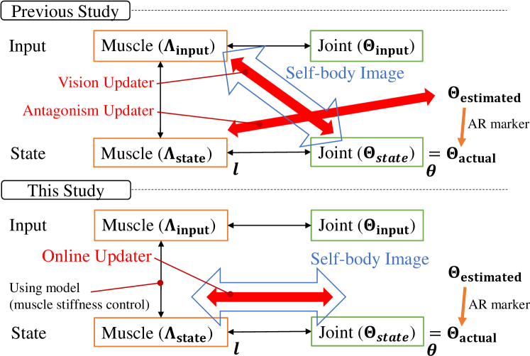
Figure 3: Difference of the network configuration between previous study [10] and this study.

III-C Initial Training of Self-body Image Using a Geometric Model

First, we train IJMM using the geometric model which linearly expresses muscle routes by the start point, relay points, and end point (the right figure of Fig. 1). We move joints of the geometric model variously in the range of the joint angle limit, calculate relative muscle lengths from the initial posture (all joint angles are $\bm{0}$ as shown in the right figure of Fig. 1), and train IJMM using these pair data of joint angles $\bm{\theta}_{rand}$ and muscle lengths $\bm{f}_{geo}(\bm{\theta}_{rand})$ (the upper right figure of Fig. 2). Second, regarding MRCM, we approximate the relationship between muscle tension and muscle elongation $\bm{L}_{e}$ with an exponential function using a test sample of one muscle. Then we make a dataset of joint angles $\bm{\theta}_{rand}$, muscle tensions $\bm{T}_{rand}$, and compensating value of muscle lengths $-\bm{L}_{e}(\bm{f}_{geo,abs}(\bm{\theta}_{rand}),\bm{T}_{rand})$ considering the elongation of the Dyneema in proportion to the absolute muscle lengths, and train MRCM (the lower right of Fig. 2). In these procedures, $\bm{f}_{geo}$ calculates relative muscle lengths from the initial posture, and $\bm{f}_{geo,abs}$ calculates absolute muscle lengths, from the geometric model. The current IJMM approximates the muscle routes along bone structures linearly, and the current MRCM cannot consider influences of muscle interferences, the soft foam cover, structure deformation, etc., so we need to update the self-body image using the actual robot sensor information.

III-D Online Learning of Self-body Image Using the Actual Robot

First, the data used for the online learning of self-body image is shown as below,

$$\bm{\theta}_{vision} =IK(\bm{\theta}_{initial}=\bm{\theta}_{est},\bm{P}_{target}=\bm{P}_{vision})$$ (2)

$$\bm{\theta}_{actual} =\bm{\theta}_{potentio}\;\;\textrm{or}\;\;\bm{\theta}_{vision}$$ (3)

$$(\bm{\theta}_{update} ,\bm{l}_{update})=(\bm{\theta}_{actual},\bm{l}_{m}-\bm{g}(\bm{\theta}_{actual},\bm{T}_{m}))$$ (4)

$$(\bm{\theta}_{update} ,\bm{T}_{update},\bm{l}_{update})=$$

$$\quad(\bm{\theta}_{actual},\bm{T}_{m},\bm{l}_{m}-\bm{f}_{ideal}(\bm{\theta}_{actual}))$$ (5)

where $\bm{l}_{m}(\bm{l}_{measured})$ is muscle lengths measured by encoders in muscle motors, $\bm{T}_{m}(\bm{T}_{measured})$ is muscle tensions measured by loadcells in muscle modules, $\bm{\theta}_{vision}$ is the estimated actual joint angles using vision implemented in [9] (solve inverse kinematics (IK) by setting the initial value $\bm{\theta}_{initial}$ as the estimated joint angles $\bm{\theta}_{est}$ and the target value $\bm{P}_{target}$ as the position of AR marker attached to the end effector $\bm{P}_{vision}$), $\bm{\theta}_{potentio}$ is the joint angles of potentiometers in the joint modules of [15], and $\{\bm{\theta,T,l}\}_{update}$ is the data used for the online learning. We use $\bm{\theta}_{potentio}$ as $\bm{\theta}_{actual}$, because each joint has potentiometers, which is one feature of Musashi used in this study. However, when the humanoid has no joint angle sensors like Kengoro [3], the online learning can be done by using $\bm{\theta}_{vision}$. Because the self-body image in this study describes the relationship of measured joint angles, muscle tensions, and muscle lengths, the online updater in Eq. 4 updates IJMM, which is the ideal relationship between joint angles and muscle lengths, by removing the influence of MRCM, and the online updater in Eq. 5 updates MRCM, which is the compensation value of muscle elongation and muscle route changes by muscle tensions, by removing the influence of IJMM. Also, this updater generates data for online learning at 2 Hz when the current joint angles or muscle lengths deviate from the previously learned data.

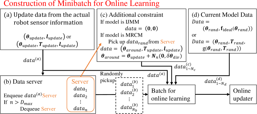
Figure 4: Data accumulation and augmentation of the actual robot sensor information for generation of minibatch for the stable online learning of self-body image.

Next, we show how to accumulate and augment the actual robot sensor information for the generation of minibatch for online learning in Fig. 4. In procedure (a), the data from the actual robot sensor information for the online learning is extracted as shown in Eq. 4 – Eq. 5. After that, the data obtained from (a) is accumulated in the data server of (b). Procedure (c) generates the data which adds the necessary limitation to the network structure of IJMM and MRCM. In the case of IJMM, because the relative muscle lengths are $\bm{0}$ when all joint angles are $\bm{0}$, (c) generates the data $(\bm{0},\bm{0})$. In the case of MRCM, because the nonlinear elastic relationship between muscle lengths and muscle tensions does not change greatly according to joint angles, (c) generates the data $(\bm{\theta}_{around},\bm{T}_{update},\bm{l}_{update})$. $\{\bm{\theta},\bm{T},\bm{l}\}_{update}$ is the actual robot sensor data extracted from the data server of (b), and $\bm{\theta}_{around}$ is obtained by adding random values following a normal distribution with an average of $0$ and a dispersion of $\delta\bm{\theta}_{div}$ to $\bm{\theta}_{update}$. Procedure (d) generates data by inputting $\bm{\theta},\bm{T}$ randomly into the current model and obtaining the output. The data is restricted by the fact that the data space other than obtained sensor data should not change from the current model. Finally, we extract one piece of data from (a), $N_{b},N_{c},N_{d}$ numbers of data from (b), (c), and (d), respectively, and generate a minibatch for online learning by compiling them together. In this study, we set $N_{b}=10,N_{c}=5,N_{d}=5$.

III-E Safety Mechanism Considering Muscle Tension and Temperature

In order to move the musculoskeletal humanoid for a long time while acquiring self-body image, it is important to prevent damage to the muscle motor by unintended high muscle tension and burnout of the muscle motor by high motor temperature. Therefore, we adjust the target muscle length to suppress the unintended high muscle tension and temperature as shown below,

$$\delta{l}= K_{T}\textrm{max}(T-T_{lim},0)+K_{C}\textrm{max}(C-C_{lim},0)$$

$$\delta{l}_{t+1}= \delta{l}_{t}+\textrm{max}(-\delta{l}_{lim},\textrm{min}(\delta{l}_{lim},\delta{l}-\delta{l}_{t}))$$

$$l_{target}= l_{target}+\delta{l}_{t+1}$$ (6)

where $l_{target}$ is the target muscle length, $\delta{l}$ is the ideal relative change of $l_{target}$, $T,C$ are the current muscle tension and temperature, $K_{T},K_{C}$ are the gains that inhibit $T$ and $C$, respectively, $T_{lim},C_{lim}$ are the threshold values for the inhibition of the rise in $T$ and $C$, $\delta{l}_{lim}$ is the limitation threshold of the change in relative muscle length for the motor not to vibrate, and $\delta{l}_{t+1}$ is the regulated relative change of muscle length which is sent at the current step. In this study, we set $K_{T}=1.0$ [mm/N], $K_{C}=1.0$ [mm/${}^{\circ}\textrm{C}$], $T_{lim}=200$ [N], $C_{lim}=60$ [${}^{\circ}\textrm{C}$], $\delta{l}_{lim}=0.01$ [mm], and this safety mechanism runs every 8 msec. This safety mechanism can inhibit high muscle tension, and cope with the case in which muscle tension is not high but the muscle temperature rises gradually, though the tracking ability of joint angles deteriorates to a certain degree.

IV Position, Torque, and Variable Stiffness Control Using Self-body Image

IV-A Position Control

First, we will explain position control using the self-body image. In this study, we move Musashi using muscle stiffness control [16] as shown below,

$$\bm{T}_{target}=\bm{T}_{bias}+\textrm{max}(\bm{0},K_{stiff}(\bm{l}-\bm{l}_{target}))$$ (7)

where $\bm{T}_{target}$ is the target muscle tension, $\bm{T}_{bias}$ is the bias term of the muscle stiffness control, and $K_{stiff}$ is the software muscle stiffness. In order to realize the intended joint angles, we need to decide $\bm{l}_{target}$ in Eq. 7, and this is done as shown below,

$$\bm{l}_{soft}(\bm{T}) =-(\bm{T}-\bm{T}_{bias})/K_{stiff}$$ (8)

$$\bm{l}_{target} =\bm{f}(\bm{\theta}_{target},\bm{T}_{const})+\bm{l}_{soft}(\bm{T}_{const})$$ (9)

$$\bm{l}_{target} =\bm{f}(\bm{\theta}_{target},\bm{T}_{measured})+\bm{l}_{soft}(\bm{T}_{measured})$$ (10)

where $\bm{f}(\bm{\theta},\bm{T})$ is the self-body image, $\bm{T}_{const}$ is constant muscle tension, and $\bm{l}_{soft}$ is the compensation values of software muscle elasticity from $\bm{l}_{target}$ by muscle stiffness control. In Eq. 9, we move the musculoskeletal humanoid using the target joint angles and constant muscle tension. However, although this movement can realize the target joint angles to a certain degree, the robot cannot move to the target posture completely because the target muscle tension is impossible to realize. Then, in Eq. 10, when we set the current measured muscle tensions to the target muscle tensions, they become the necessary muscle tensions to approximately realize the target joint angles. Ideally the robot can completely realize the target joint angles by continuing the feedback of the current measured muscle tensions, but in actuality, there is an error between the self-body image and the actual robot, so the current muscle tensions can diverge or converge to minimum muscle tensions $\bm{T}_{bias}$, which is not practical, if we continue the feedback of Eq. 10. Also, although there are many combinations of target muscle tensions which can realize the target joint angles due to the redundant muscle arrangements, by setting the $\bm{T}_{const}$ to the minimum muscle tension $\bm{T}_{bias}$, the robot can realize the target joint angles by minimum muscle tensions.

IV-B Torque Control

Next, by using this self-body image, we can conduct torque control of musculoskeletal structures. The basic method is the joint torque control using muscle tension [17]. By the acquisition of self-body image, the torque control [17] becomes better, because a more accurate muscle Jacobian than the one of the geometric model can be obtained by differentiating the self-body image. Also, the acquisition of self-body image makes the joint angle estimation more correct [9, 10], and the actual joint angles can follow the target joint angles more accurately.

IV-C Variable Stiffness Control

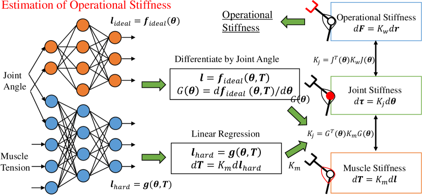
Figure 5: Estimation of operational hardware stiffness using self-body image.

IV-C1 Estimation of Self-body Stiffness

First, we estimate operational hardware stiffness as shown in Fig. 5. In order to estimate the operational stiffness, joint Jacobian $J$, muscle Jacobian $G$, and muscle stiffness $K_{m}$ are necessary. First, we can obtain the joint Jacobian from the geometric model, as with ordinary axis-driven humanoids. Second, muscle Jacobian can be obtained by differentiating the IJMM of the self-body image by the joint angles. Third, muscle stiffness can be obtained using linear regression between the change in muscle tensions and the change in output of the MRCM. Therefore, the operational stiffness can be estimated by multiplying muscle stiffness by muscle Jacobian and joint Jacobian.

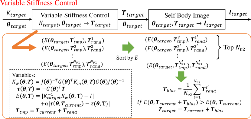
Figure 6: Control of operational hardware stiffness using self-body image.

IV-C2 Control of Self-body Stiffness

The basic system of variable stiffness control is shown in the upper figure of Fig. 6: we set the target joint angles and target operational stiffness, calculate the target muscle tension using the method we will propose in this subsection, calculate the target muscle lengths from self-body image by inputting the calculated muscle tensions, and send them to the actual robot. The details of variable stiffness control is shown in the lower figure of Fig. 6. First, we make $\bm{T}_{tmp}$ by adding $\bm{T}_{rand}$, which is a random value within a certain range ($-20\sim 20$ [N] in this study), to the current muscle tensions $\bm{T}_{current}$, and accumulate $N_{v1}$ data pairs of $\bm{T}_{rand}$ and evaluation value $E(\bm{\theta}_{target},\bm{T}_{tmp})$ based on the equation as shown below,

$$\bm{T}_{tmp}= \bm{T}_{current}+\bm{T}_{rand}$$

$$K_{w}(\bm{\theta},\bm{T})= J(\bm{\theta})^{-T}G(\bm{\theta})^{T}K_{m}(\bm{\theta},\bm{T})G(\bm{\theta})J(\bm{\theta})^{-1}$$

$$\bm{\tau}(\bm{\theta},\bm{T})= -G(\bm{\theta})^{T}\bm{T}$$

$$E(\bm{\theta},\bm{T})= |K^{-1}_{target}K_{w}(\bm{\theta},\bm{T})-I|$$

$$+\alpha|\bm{\tau}(\bm{\theta},\bm{T}_{current})-\bm{\tau}(\bm{\theta},\bm{T})|$$ (11)

where $K_{w}(\bm{\theta},\bm{T})$ is the calculated operational stiffness, $K_{target}$ is the target operational stiffness, $J(\bm{\theta})$ is the joint Jacobian, $G(\bm{\theta})$ is the muscle Jacobian, $\bm{K}_{m}$ is the muscle stiffness, $\bm{\tau}(\bm{\theta},\bm{T})$ is the joint torque, $\alpha$ is a weight constant, and $|\cdot|$ expresses L2 norm. The evaluation value $E(\bm{\theta},\bm{T})$ sums up the values that express how the calculated operational stiffness is close to the target operational stiffness when $\bm{T}=\bm{T}_{target}$, and how the calculated joint torques are close to the current joint torques when $\bm{T}=\bm{T}_{current}$, by the weight of $1:\alpha$. We sort the accumulated data in ascending order of the value $E$, and set $\bm{T}_{bias}$ as the average $\bm{T}_{rand}$ of $N_{v2}$ ($N_{v1}>N_{v2}$) data from the top. Then, we replace the $\bm{T}_{target}$ by $\bm{T}_{current}+\bm{T}_{bias}$, when the value $E(\bm{\theta}_{target},\bm{T}_{current}+\bm{T}_{bias})$ is smaller than $E(\bm{\theta}_{target},\bm{T}_{current})$. We repeat this step $N_{v3}$ times, input the final calculated value of $\bm{T}_{target}$ into the self-body image, and obtain the target muscle length. When $N_{v2}=1$, this method is a hill climbing method, and when $N_{v2}>1$, the stiffness search becomes more stable. In this study, we set $\alpha=0.02,N_{v1}=10,N_{v2}=2$, and $N_{v3}=50$.

Although we change the operational stiffness in this section, this method can also be applied to change the joint stiffness.

V Experiments

In all experiments, the neural networks have three layers: input, hidden, and output layers. The number of units in the hidden layer is 1000, and the activation function is Sigmoid.

V-A Comparison of self-body image acquisition methods

First, we will conduct an experiment to compare the self-body image acquisition methods of the previous study [10] and this study. In the previous study, self-body image was learned in a state without external force, and then was learned in a state with external force. In this study, first, we set the target joint angles $\bm{\theta}_{target}$ randomly in the range of the joint angle limits, set the $\bm{T}_{const}$ as $\bm{T}_{bias}$, and sent target muscle lengths obtained by Eq. 9 to the robot over 5 sec. Second, we sent the target muscle lengths obtained by Eq. 10 using the same target joint angles over 2 sec. Third, we set $\bm{T}_{const}$ as the random value from $\bm{T}_{bias}$ to $\bm{T}_{lim}$, and sent muscle lengths obtained by Eq. 9 again using the same target joint angles over 3 sec. By repeating these 3 steps, the space of joint angles and muscle tensions of the self-body image is learned efficiently. We used the 5 DOFs of the 3 DOFs shoulder and 2 DOFs elbow in Musashi for the evaluation, including a total of 10 muscles (we express muscles by the numbers $\#1\sim\#10$ shown in the right figure of Fig. 1, which include 1 polyarticular muscle). We applied the previous study to the right arm and applied this study to the left arm, and evaluated at the same time.

We show the result in Fig. 7. RMSE is the Root Mean Squared Error of the difference between the current and estimated joint angles. When comparing the transition of RMSEs and their linear regressions in these two studies, both of the RMSEs decrease slowly, and the slope in this study is larger than the one in the previous study. This is because the two updaters of the previous study slightly compete and the self-body image is adjusted to the current sensor information too much due to lack of data accumulation. Also, we added external force at 500 sec. There is no use of torque controller. After that, by setting two different target joint angles, RMSE in the previous study rose rapidly. This is because the self-body image is adjusted to the current joint angles too much, and so the joint angle estimation goes in an unintended direction when moving to a great extent.

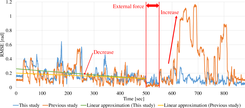
Figure 7: Comparison experiment of self-body image acquisition between the previous study and this study.

V-B Long-time Self-body Image Acquisition

We conducted a long-time self-body image acquisition experiment lasting 3 hours. We show the result in Fig. 8. In the upper figure of Fig. 8, RMSE is the Root Mean Squared Error of the difference between the current and target joint angles, and the black line expresses the average RMSE of 4 minutes. We can see that the average RMSE gradually decreased from about 0.3 rad to 0.08 rad until at about 40 minutes by the online acquisition of the correct self-body image. Although the O-ring of muscle $\#6$ ruptured at 42 minutes and the RMSE increased to about 0.2 rad, the RMSE gradually decreased due to the redundancy of muscles and the online learning of self-body image, expressing the benefit of redundant muscles on the musculoskeletal structure well. After that, muscles $\#2$ and $\#3$ ruptured at about 150 minutes, the major muscles required to raise the shoulder in the roll direction vanished, and RMSE increased rapidly. Regarding the muscle temperatures, the temperature remained stable under 70 ${}^{\circ}\textrm{C}$ due to the safety mechanism of Eq. 6. Also, because we did not set self-collision avoidance, at 140 minutes, target joint angles were set to values that caused the arm to sink into the self-body, and muscle temperatures rose rapidly. However, due to the safety mechanism, the robot could keep moving without exceeding the limit of muscle temperature $C_{burn}$ (90 ${}^{\circ}\textrm{C}$) which is the limit for the prevention of motor burnout.

The main reason why the average RMSE did not fall under about 0.08 rad is the hysteresis of muscles. MusashiLarm has a complex muscle structure, large friction between muscles, between muscle and bone, between muscle and pulley, etc., and the final joint angles change according to the direction of movement.

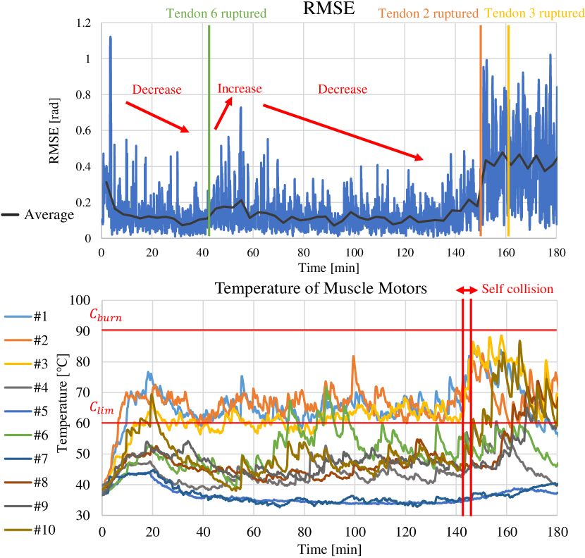
Figure 8: Transition of Root Mean Squared Error (RMSE) of the difference between target and current joint angles and muscle temperature in the long-time self-body image acquisition experiment lasting 3 hours.

V-C Dumbbell Raise Experiment

We conducted a dumbbell (3 kg) raise experiment by position control using the self-body image, while running its online learning. We show the appearance in the upper figure of Fig. 9, and show the transition of the dumbbell height in the lower figure of Fig. 9. When raising the dumbbell several times, the relationship of muscle lengths, muscle tension, etc. of the dumbbell raise is incorporated into the self-body image, so Musashi was gradually able to raise the dumbbell to the target height of 730 mm.

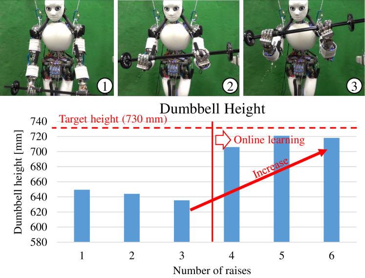
Figure 9: Result of dumbbell raise experiment. Lower graph expresses the transition of the dumbbell height.

V-D Variable Stiffness Control Using Self-body Image

First, we conducted the evaluation of the variable stiffness control. We set $\bm{\theta}_{target}$ as $({S}_{r},{S}_{p},{S}_{y},{E}_{p},{E}_{y})=(45,0,0,-90,0)$ [deg], and conducted experiments to change the operational stiffness as intended ($S$ means the shoulder, $E$ means the elbow, and $rpy$ means the roll, pitch, and yaw rotation. These symbols are also used in subsequent experiments). The result is shown in Fig. 10. Each stiffness ellipsoid in the upper graphs of Fig. 10 represents the operational displacement of the hand when $|\bm{F}|=10$ [N]. In Sample 1, we set the target stiffness $K_{target}$ (Target Value) as a stiffness twice that of the current stiffness (Current Value), and searched for target muscle tensions by the method of Section IV-C. The transition of $E(\bm{\theta},\bm{T})$ in Sample 1 when searching for target muscle tensions is shown in the lower graph of Fig. 10, showing that this method could make the self-body stiffness close to the target stiffness, while inhibiting the error between current and calculated joint torques (in this graph, we display the value $E$ if $E(\bm{\theta}_{target},\bm{T}_{current}+\bm{T}_{bias})>E(\bm{\theta}_{target},\bm{T}_{current})$). When we move the actual robot using $\bm{T}_{target}$, which realizes the final stiffness (Calculated Value) calculated by the method, we can observe the final current stiffness of the actual robot (Actual Value). In Sample 1, $\bm{T}_{target}$, which realizes the target stiffness, could not be obtained, but this method succeeded in making the current stiffness close to the target stiffness. Also, the stiffness ellipsoids of Calculated Value and Actual Value were almost the same, and it shows that the self-body image was learned correctly. In Sample 2, we set the target stiffness by changing the scale and slope of the current stiffness ellipsoid. As a result of the search, the same scale of the target stiffness ellipsoid was realized, but the slope was not, because there was no solution to realize the target stiffness and the method selected the best choice.

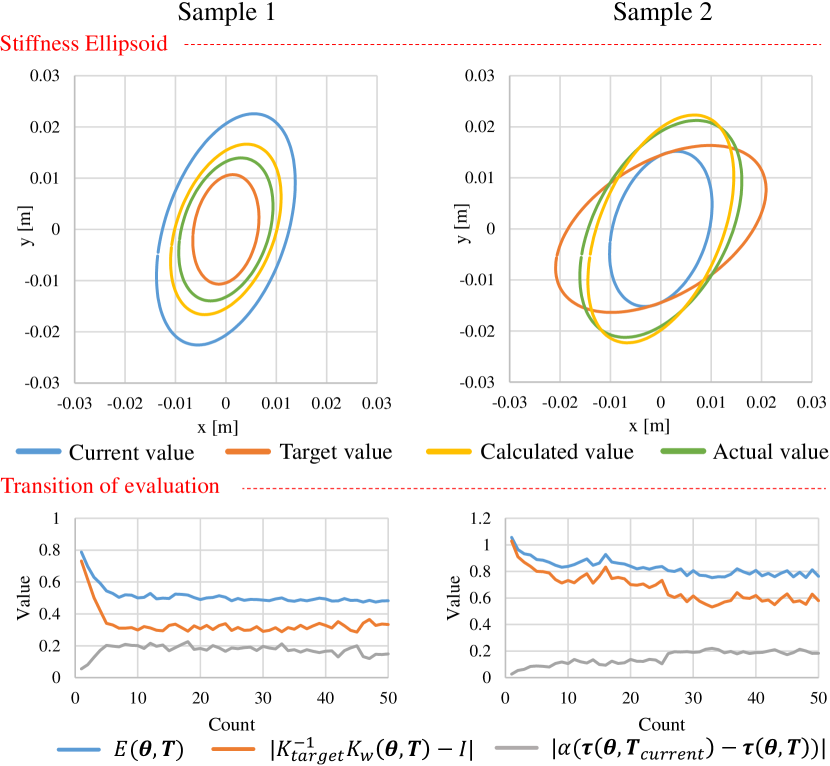
Figure 10: Stiffness ellipsoid and transition of evaluation in the evaluation experiment of variable stiffness control using self-body image.

Second, we verified to what extent the theoretical stiffness ellipsoid calculated by the method in Section IV-C matches the actual stiffness ellipsoid. We set $\bm{\theta}_{target}$ as $({S}_{r},{S}_{p},{S}_{y},{E}_{p},{E}_{y})=(0,30,0,-60,0)$ [deg], which is the posture in which the body stiffness can be measured easily, and created a state of low stiffness and high stiffness by the method in Section IV-C. Then, we added 10 N force to the end effector on the $xy$ plane, while measuring the value by a forcegauge, from 8 directions equally dividing 360 deg, and measured the displacement of the end effector by potentiometers. The result is shown in Fig. 11. When the body stiffness is low or high, we can see that the theoretical and actual ellipsoid match to a certain degree. The error between the theoretical and actual value is considered to be due to the remaining difference between the acquired self-body image and the actual robot, and the hysteresis by friction as above.

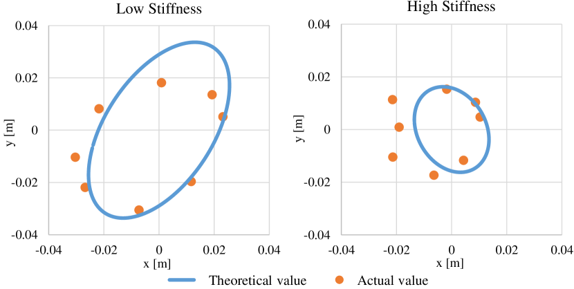
Figure 11: Stiffness ellipsoid in the evaluation experiment of variable stiffness estimation using self-body image.

V-E Impact Correspondence Experiment

We conducted an impact correspondence experiment using variable stiffness control. The joint angles were set as $({S}_{r},{S}_{p},{S}_{y},{E}_{p},{E}_{y})=(-45,-30,-20,-60,0)$ [deg], a 5 kg ball was dropped from 1 m above and 0.15 m in front of the elbow with the hands clasped together, and the transitions of muscle tensions and joint angles between low stiffness and high stiffness were compared. The movement of the dual arm in this experiment is shown in Fig. 12, and the transitions of muscle tensions and joint angles of the left arm are shown in Fig. 13. From Fig. 12, we can see that the arms moved to a great extent when the stiffness was low, and the displacement of the arms was not as large when the stiffness was high. Additionally, in the lower graph of Fig. 13, we can see that both displacements of joint angles in Shoulder-p and Elbow-p become small in the high stiffness state. Also, in the upper figure of Fig. 13, although the evaluation of muscle tensions is difficult because the initial muscle tensions are different between low and high stiffness, the maximum muscle tension is about 150 N in low stiffness and is about 250 N in high stiffness, indicating that the low stiffness state can absorb sudden impact.

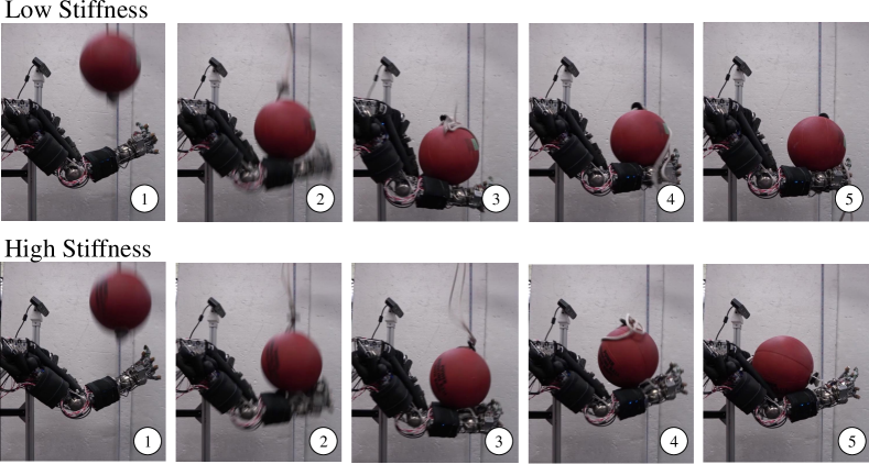
Figure 12: Impact correspondence experiment with variable stiffness control.

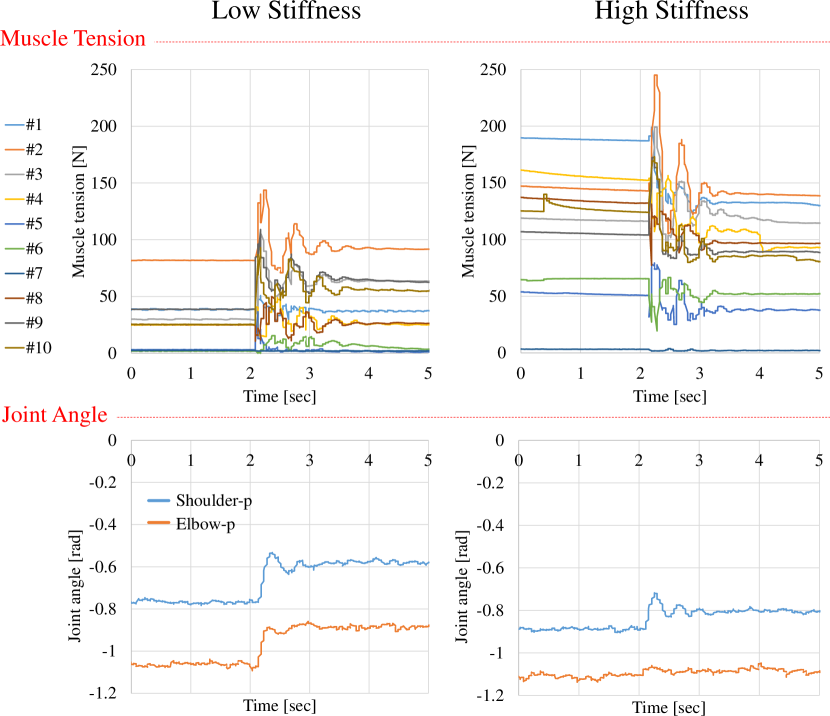
Figure 13: Transition of muscle tensions and joint angles in the impact correspondence experiment with variable stiffness control.

VI CONCLUSION

In this study, we proposed a method for long-time self-body image acquisition, and position, torque, and variable stiffness control using the self-body image. For long-time self-body image acquisition, we considered simplifying the online updater for stable learning, accumulating and augmenting the actual robot sensor information without wasting it, and including a safety mechanism to inhibit high muscle tension and temperature, and we succeeded in conducting a 3 hour learning experiment. Also, by using the self-body image, we realized position control using 2 stage feedback of muscle tension, torque control using muscle Jacobian calculated from the differentiation of the self-body image, and variable stiffness control using hill-climb method.

In future works, we would like to propose further structures of self-body image considering the hysteresis of muscles and dynamic movements.

References

- [1] Y. Nakanishi, S. Ohta, T. Shirai, Y. Asano, T. Kozuki, Y. Kakehashi, H. Mizoguchi, T. Kurotobi, Y. Motegi, K. Sasabuchi, J. Urata, K. Okada, I. Mizuuchi, and M. Inaba, “Design Approach of Biologically-Inspired Musculoskeletal Humanoids,” International Journal of Advanced Robotic Systems, vol. 10, no. 4, pp. 216–228, 2013.
- [2] S. Wittmeier, C. Alessandro, N. Bascarevic, K. Dalamagkidis, D. Devereux, A. Diamond, M. Jäntsch, K. Jovanovic, R. Knight, H. G. Marques, P. Milosavljevic, B. Mitra, B. Svetozarevic, V. Potkonjak, R. Pfeifer, A. Knoll, and O. Holland, “Toward Anthropomimetic Robotics: Development, Simulation, and Control of a Musculoskeletal Torso,” Artificial Life, vol. 19, no. 1, pp. 171–193, 2013.
- [3] Y. Asano, T. Kozuki, S. Ookubo, M. Kawamura, S. Nakashima, T. Katayama, Y. Iori, H. Toshinori, K. Kawaharazuka, S. Makino, Y. Kakiuchi, K. Okada, and M. Inaba, “Human Mimetic Musculoskeletal Humanoid Kengoro toward Real World Physically Interactive Actions,” in Proceedings of the 2016 IEEE-RAS International Conference on Humanoid Robots, 2016, pp. 876–883.
- [4] S. Hirose and S. Ma, “Coupled tendon-driven multijoint manipulator,” in Proceedings of the 1991 IEEE International Conference on Robotics and Automation, 1991, pp. 1268–1275.
- [5] H. G. Marques, , C. Maufroy, A. Lenz, K. Dalamagkidis, and U. Culha, “MYOROBOTICS: a modular toolkit for legged locomotion research using musculoskeletal designs,” in Proceedings of 6th International Symposium on Adaptive Motion of Animals and Machines, 2013.
- [6] I. Mizuuchi, Y. Nakanishi, T. Yoshikai, M. Inaba, H. Inoue, and O. Khatib, “Body Information Acquisition System of Redundant Musculo-Skeletal Humanoid,” in Experimental Robotics IX, 2006, pp. 249–258.
- [7] S. Ookubo, Y. Asano, T. Kozuki, T. Shirai, K. Okada, and M. Inaba, “Learning Nonlinear Muscle-Joint State Mapping Toward Geometric Model-Free Tendon Driven Musculoskeletal Robots,” in Proceedings of the 2015 IEEE-RAS International Conference on Humanoid Robots, 2015, pp. 765–770.
- [8] Y. Motegi, T. Shirai, T. Izawa, T. Kurotobi, J. Urata, Y. Nakanishi, K. Okada, and M. Inaba, “Motion control based on modification of the Jacobian map between the muscle space and work space with musculoskeletal humanoid,” in Proceedings of the 2012 IEEE-RAS International Conference on Humanoid Robots, 2012, pp. 835–840.
- [9] K. Kawaharazuka, S. Makino, M. Kawamura, Y. Asano, K. Okada, and M. Inaba, “Online Learning of Joint-Muscle Mapping using Vision in Tendon-driven Musculoskeletal Humanoids,” IEEE Robotics and Automation Letters, vol. 3, no. 2, pp. 772–779, 2018.
- [10] K. Kawaharazuka, S. Makino, M. Kawamura, A. Fujii, Y. Asano, K. Okada, and M. Inaba, “Online Self-body Image Acquisition Considering Changes in Muscle Routes Caused by Softness of Body Tissue for Tendon-driven Musculoskeletal Humanoids,” in Proceedings of the 2018 IEEE/RSJ International Conference on Intelligent Robots and Systems, 2018, pp. 1711–1717.
- [11] H. Kobayashi, K. Hyodo, and D. Ogane, “On Tendon-Driven Robotic Mechanisms with Redundant Tendons,” The International Journal of Robotics Research, vol. 17, no. 5, pp. 561–571, 1998.
- [12] M. V. Weghe, M. Rogers, M. Weissert, and Y. Matsuoka, “The ACT Hand: design of the skeletal structure,” in Proceedings of the 2004 IEEE International Conference on Robotics and Automation, 2004, pp. 3375–3379.
- [13] C. Paul, F. J. Valero-Cuevas, and H. Lipson, “Design and control of tensegrity robots for locomotion,” IEEE Transactions on Robotics, vol. 22, no. 5, pp. 944–957, 2006.
- [14] R. Niiyama, S. Nishikawa, and Y. Kuniyoshi, “Athlete Robot with applied human muscle activation patterns for bipedal running,” in Proceedings of the 2010 IEEE-RAS International Conference on Humanoid Robots, 2010, pp. 498–503.
- [15] K. Kawaharazuka, S. Makino, X. Chen, A. Fujii, M. Kawamura, T. Makabe, M. Onitsuka, Y. Asano, K. Okada, K. Kawasaki, and M. Inaba, “Design of a Musculoskeletal Upper Limb with Pseudo Ball Joint Modules for the Control of Redundant Nonlinear Elastic Elements,” in 2017 JSME Conference on Robotics and Mechatronics, 2018, pp. 2A2–G09.
- [16] T. Shirai, J. Urata, Y. Nakanishi, K. Okada, and M. Inaba, “Whole body adapting behavior with muscle level stiffness control of tendon-driven multijoint robot,” in Proceedings of the 2011 IEEE International Conference on Robotics and Biomimetics, 2011, pp. 2229–2234.
- [17] M. Kawamura, S. Ookubo, Y. Asano, T. Kozuki, K. Okada, and M. Inaba, “A Joint-Space Controller Based on Redundant Muscle Tension for Multiple DOF Joints in Musculoskeletal Humanoids,” in Proceedings of the 2016 IEEE-RAS International Conference on Humanoid Robots, 2016, pp. 814–819.