Effective-one-body waveform model for non-circularized, planar, coalescing black hole binaries: the importance of radiation reaction

Abstract

We present an updated version of the TEOBResumS-Dali effective-one-body (EOB) waveform model for spin aligned binaries on non-circularized orbits. Recently computed 4PN (nonspinning) terms are incorporated in the waveform and radiation reaction. The model is informed by a restricted sample ($\sim 60$) of spin-aligned, quasi-circular, Numerical Relativity (NR) simulations. In the quasi-circular limit, the model displays EOB/NR unfaithfulness ${\bar{\cal F}}^{\rm max}_{\rm EOBNR}\lesssim 10^{-2}$ (with median  $1.06\times 10^{-3}$) (with Advanced LIGO noise and in the total mass range $10-200M_{\odot}$) for the dominant $\ell=m=2$ mode all over the 534 spin-aligned configurations available through the Simulating eXtreme Spacetime catalog of NR waveforms. Similar figures are also obtained with the 28 public eccentric SXS simulations and good compatibility between EOB and NR scattering angles is found. The quasi-circular limit of TEOBResumS-Dali is also found to be highly consistent with the TEOBResumS-GIOTTO quasi-circular model. We then systematically explore the importance of NR-tuning also the radiation reaction of the system. When this is done, the median of the distribution of quasi-circular ${\bar{\cal F}}^{\rm max}_{\rm EOBNR}$ is lowered to $3.92\times 10^{-4}$, though balanced by a tail up to $\sim 0.1$ for large, positive spins. The same is true for the eccentric-inspiral datasets. We conclude that an improvement of the analytical description of the spin-dependent flux (and its interplay with the conservative part) is likely to be the cornerstone to lower the EOB/NR unfaithfulness below the $10^{-4}$ level all over the parameter space, thus grazing the current NR uncertainties as well as the expected needs for next generation of GW detector like Einstein Telescope.

I Introduction

Prompted by the desire of obtaining models able to include a large class of physical effects, the last few years have seen an increasing interest from the gravitational waves (GW) community in the construction of accurate waveform models incorporating orbital eccentricity and in general configurations that go beyond the standard quasi-circular case. These efforts have been particularly vibrant within the Effective-One-Body (EOB) framework, with many studies [1, 2, 3] proposing different techniques to model non-circularized binaries. In particular, the TEOBResumS-Dali model [2] immediately proved to be sufficiently mature to pioneer several parameter estimation studies involving both bound configurations (i.e. eccentric inspirals) [4] and unbound ones (i.e. scattering or dynamical capture) [5]. This model is built upon the crucial understanding that the factorized and resummed EOB quasi-circular waveform and radiation reaction [6] can be generalized to the case of eccentric binaries by simply considering generic Newtonian prefactors in the waveform and fluxes [2, 7]. Although this procedure neglects some (high-order) physical effect, it proved sufficiently accurate in several context. The idea, technically complemented by the analytical implementation of (high-order) time derivatives via an iterative procedure [2, 8], was thoroughly tested versus a large amount of numerical data both in the comparable mass [9, 5, 7, 10, 11, 12, 13] and in the large mass ratio limit [14, 15], notably also exploring the effect of higher-order PN terms in radiation reaction and waveform [16, 15, 17]. Among the many findings of this lineage of work, Refs. [2, 15] clearly proved that the Newton-factorized azimuthal part of the radiation reaction is more accurate than the 2PN-accurate one proposed in Ref. [18] (see Ref. [19] for the 3PN calculation). We note that the approach of Ref. [2] and subsequent works was not adopted in a different lineage of eccentric EOB-based models, dubbed SEOBNRv4EHM [3, 19, 20]. In this respect, while TEOBResumS-Dali was proven to be quantitatively accurate also for dynamical capture configurations as well as scattering ones [5, 11, 12], the corresponding studies involving SEOBNRv4EHM in this regime were at most qualitative [3]. The Achilles’ heel of TEOBResumS-Dali was however hidden in its quasi-circular limit, where the model was found to perform not as well as the quasi-circular TEOBResumS-GIOTTO version, especially for large, positive spins [7, 4]. This problem, related to the strong-field behavior of the radial part of the radiation reaction, ${\cal F}_{r}$ was solved, in the nonspinning case, in Ref. [13] adopting a different analytical expression for it (see Fig. 12 and discussion in Sec. IV therein). Note in this respect that Ref. [13] did not consider, on purpose, the eccentric spin case, that deserved more dedicated understanding and work.

Here we build upon the knowledge acquired in Ref. [13] and present an improved version of the TEOBResumS-Dali model in its avatar introduced in Ref. [10] (that also deals with spin-aligned binaries). The quasi-circular limit of this new version yields an excellent consistency with TEOBResumS-GIOTTO as well as with the SXS quasi-circular Numerical Relativity (NR) datasets. The model incorporates some new analytical information, namely the 4PN term in the quadrupolar waveform (and flux) recently computed in Refs. [21, 22, 23]. The availability of this new information enables a detailed investigation of the effect of minimal changes in the radiation reaction and their nonnegligible impact on the phasing. In this respect, we explore the possibility of tuning the radiation reaction to the NR data; we conclude that this will likely be needed to obtain waveform templates highly faithful to NR data (say, $\sim 10^{-4}$ level) as they are expected to be needed for Third Generation (3G) detectors.

The paper is organized as follows. In Sec. II we recall the main elements of the TEOBResumS-Dali model of Refs. [10, 13] and highlight the modifications introduced in this work. In particular, Sec. II.1 is dedicated to the factorization and resummation of the 4PN waveform of Ref. [21] following the standard EOB approach [6], while Sec. II.2 discusses the dynamics and more generally the spin sector. In Sec. III we present the new spin-aligned model, discussing in detail quasi-circular configurations, eccentric configurations as well as scattering. In Sec. IV we break new ground with respect to previous work by investigating various improvements in the model that can be obtained by NR-informing also the radiation reaction. Concluding remarks are collected in Sec. V. The main text is complemented by a few appendices. In particular, Appendix A identifies some analytical systematics related to the Padé resummation of the waveform and discusses their solution. In addition, Appendix B presents the implementation of the initial conditions for eccentric inspirals using eccentricity and mean anomaly instead of using eccentricity and frequency at the apastron as it was done in previous work.

We adopt the following notations and conventions. The black hole masses are denoted $(m_{1},m_{2})$, the mass ratio $q=m_{1}/m_{2}\geq 1$, the total mass $M\equiv m_{1}+m_{2}$, the symmetric mass ratio $\nu\equiv m_{1}m_{2}/M^{2}$ and the mass fractions $X_{i}\equiv m_{i}/M$ with $i=1,2$. The dimensionless spin magnitudes are $\chi_{i}\equiv S_{i}/m_{1}^{2}$ with $i=1,2$, and we indicate with $\tilde{a}_{0}\equiv\tilde{a}_{1}+\tilde{a}_{2}\equiv X_{1}\chi_{1}+X_{2}\chi_{2}$ the effective spin, usually called $\chi_{\rm eff}$ in the literature. Unless otherwise stated, we use geometric units with $c=G=1$.

II Analytic EOB structure: waveform and dynamics

As previously mentioned, we build upon the spin-aligned, eccentric TEOBResumS-Dalí model discussed extensively in Ref. [10] and Sec. IIIB.2 of Ref. [13], improving few key aspects of it. In this section, we discuss the analytical structure of the model. First, we focus on the pure-orbital sector, and incorporate 4PN waveform information in the $\ell=m=2$ contribution to waveform and radiation reaction. Then, we remove the next-to-next-to-leading order (NNLO) spin-square effects that were first introduced in a factorized and resummed form in Ref. [10]. This will prompt a new determination of the $(a_{6}^{c},c_{3})$ EOB flexibility parameters, that will be discussed in the following section (see Sec. III).

II.1 The 4PN factorized and resummed nonspinning waveform

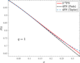
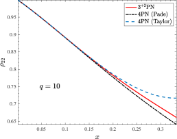
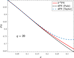
Figure 1: Comparing various approximations of the function $\rho_{22}$ for mass ratios $q=(1,10,20)$: the $3^{+2}$ PN one used in the standard implementation of TEOBResumS; the $\rho_{22}$ at 4PN accuracy, resummed with the $(2,2)$ Padé approximant; the 4PN, Taylor-expanded, function. Note the consistency between the $3^{+2}$ and the 4PN resummed as well as their weak dependence on the mass ratio.

In order to be employed in EOB models, PN expression typically need to be recast in factorized and resummed form [24, 6]. This is particularly important for the radiation reaction, where the factorization and resummation of the fluxes is crucial to obtain a faithful description of the dynamics. Here, we start from the 4PN accurate waveform obtained in Refs. [23, 22, 21] and recast it in the desired form of [6], following the procedure of Ref. [25].

Let us first recall our notation. The multipolar expansion of the strain waveform is

$$h_{+}-ih_{\times}=\dfrac{1}{D_{L}}\sum_{\ell=2}^{\infty}\sum_{m=-\ell}^{\ell}h_{{\ell m}}{}_{-2}Y_{{\ell m}}\,,$$ (1)

where $D_{L}$ is the luminosity distance and ${}_{-2}Y_{{\ell m}}$ are the $s=-2$ spin-weighted spherical harmonics. For each multipolar mode, the circular waveform is factorized as

$$h_{\ell m}=h_{\ell m}^{N}\hat{h}_{\ell m}\ ,$$ (2)

where $h_{\ell m}^{N}$ is the Newtonian prefactor (given in closed form e.g. in Ref. [6]) and $\hat{h}_{\ell m}$ is the PN correction. Following [6], this latter is factorized as

$$\hat{h}_{\ell m}=\hat{S}_{\rm eff}T_{\ell m}e^{i\delta_{\ell m}}(\rho_{\ell m})^{\ell}\ ,$$ (3)

where $S_{\rm eff}$ is the effective source, $T_{\ell m}$ is the tail factor [6], while $\rho_{\ell m}$ and $\delta_{\ell m}$ are the residual amplitude and phase corrections. The tail factor explicitly reads

$$T_{\ell m}=\dfrac{\Gamma\left(\ell+1-2{\rm i}\hat{\hat{k}}\right)}{\Gamma(\ell+1)}e^{\pi\hat{\hat{k}}}e^{2{\rm i}\hat{\hat{k}}\log(2kr_{0})}\ .$$ (4)

Indicating with $E$ the energy along a circular orbit of frequency $\Omega$, we have $\hat{\hat{k}}\equiv mE\Omega$, $k\equiv m\Omega$ and $r_{0}=2/\sqrt{e}$ [26]. The formula above is specified to the $\ell=m=2$ case starting from Eq. (11) of Ref. [21] (where $\hat{h}_{22}\equiv H_{22}$ therein) and $E$, at 4PN accuracy, given by Eq. (3) therein. Note that $x\equiv(M\Omega)^{2/3}$. The factorization (following the procedure and conventions of Ref. [25] for consistency with the results given in [21]) yields the following 4PN-accurate $\rho_{22}$ function:

$$\rho_{22}^{\rm 4PN}(x) =1+\left(-\dfrac{43}{42}+\dfrac{55}{84}\nu\right)x+\left(-\dfrac{20555}{10584}-\dfrac{33025}{21168}\nu+\dfrac{19583}{42336}\nu^{2}\right)x^{2}$$

$$+\bigg{[}\dfrac{1556919113}{122245200}-\frac{428}{105}\text{eulerlog}_{2}(x)+\left(\frac{41\pi^{2}}{192}-\frac{48993925}{9779616}\right)\nu-\frac{6292061}{3259872}\nu^{2}+\frac{10620745}{39118464}\nu^{3}\bigg{]}x^{3}$$

$$+\bigg{[}-\frac{387216563023}{160190110080}+\text{eulerlog}_{2}(x)\left(\frac{9202}{2205}+\frac{8819}{441}\nu\right)+\left(-\frac{6718432743163}{145627372800}-\frac{9953\pi^{2}}{21504}\right)\nu$$

$$+\left(\frac{10815863492353}{640760440320}-\frac{3485\pi^{2}}{5376}\right)\nu^{2}-\frac{2088847783}{11650189824}\nu^{3}+\frac{70134663541}{512608352256}\nu^{4}\bigg{]}x^{4}\ ,$$ (5)

where $\text{eulerlog}_{m}(x)\equiv\gamma_{E}+\log(2m\sqrt{x})$. The residual phase, instead, reads:

$$\delta_{22} =\dfrac{7}{3}y^{3/2}-24\nu y^{5/2}+\dfrac{428}{105}\pi y^{3}$$

$$+\left(\dfrac{30995}{1134}\nu+\dfrac{962}{135}\nu^{2}\right)y^{7/2}-\dfrac{5536}{105}\pi\nu y^{4}\ ,$$ (6)

with $y=(E\Omega)^{2/3}$.

Once the first factorization is performed, the residual functions need to be resummed. Phase and amplitude are considered separately, and their behaviors in the high-velocity limit studied. Let us first discuss the 4PN correction to $\delta_{22}$. The analytical expression for $\delta_{22}$ implemented in TEOBResumS dates back to to Ref. [8] (see Sec. IIB.1 and Fig. 1). There, it was obtained by factorizing the leading-order (LO) part of $\delta_{22}$, $\delta_{22}^{\rm LO}=7/3y^{3/2}$, and resumming the remaining factor, $\hat{\delta}_{22}$, with a Padé $(2,2)$ approximant in the variable $v_{y}=\sqrt{y}$. In this respect, Fig. 1 of Ref. [8] illustrates that the chosen Padé approximant is effective in averaging the various PN-truncations of $\delta_{22}$. This fact by itself indicates that the resummed expression should give a representation of the function $\delta_{22}$ more robust than the truncated Taylor expansion and, as such, should be extended at the next available PN order. Attempting to follow this procedure, we compute the $\hat{\delta}_{22}$ factor, which at 4PN reads:

$$\hat{\delta}_{22} =1-\dfrac{72}{7}\nu v_{y}^{2}+\dfrac{428\pi}{245}v_{y}^{3}$$

$$+\nu\left(\dfrac{30995}{2646}+\dfrac{962}{315}\nu\right)v_{y}^{4}-\dfrac{5536\pi}{245}\nu v_{y}^{5}\ .$$ (7)

We have explored several ways of treating this expression analytically. First, one considers the straightforward, Taylor-expanded expression. If for $q=1$ it is close to the former Padé $(2,2)$ one, as $\nu$ decreases the function is found to abruptly grow as $v_{y}\to 0.3$. When moving to Padé approximants, it is natural to consider the near-diagonal ones, i.e. $P^{2}_{3}$ and $P^{3}_{2}$. However, one finds that the $P^{2}_{3}$ develops a spurious pole, while the $P^{3}_{2}$ increases again for $v_{y}\to 0.3$ when $\nu$ decreases. By contrast, the $(2,2)$ approximant remains robust and keeps the same functional shape for any choice of $\nu$. In view of these results, for robustness, we decided to neglect the new 4PN contribution to $\hat{\delta}_{22}$ and just keep using the Padé $(2,2)$ approximant.

The $\rho_{22}(x)$ function, Eq. (II.1), is similarly resummed using a Padé $(2,2)$ approximant. Following standard practice within the EOB framework [27], the $\log(x)$ functions appearing Eq. (II.1) above are treated as constant when computing the Padé approximant [28]. The $\log(x)$ are then replaced in the resulting rational function. Note that this approach is implemented for all higher order modes, as suggested in Refs. [28, 29, 30]. This choice, though simple and consistent with the low-order PN expansion, eventually introduces some qualitative incorrectness in the high-order terms as guessed by the resummation procedure. For consistency with previous work we pursue this approach in the main text of the paper. However, in Appendix A we revisit this standard choice and propose a different (though eventually more accurate) resummation strategy. To appreciate the importance of the resummation , let us compare the Padé resummed function with its Taylor-expanded expression as well as with the $\rho_{22}$ at $3^{+2}$ PN accuracy used in all implementations of TEOBResumS so far, starting from Ref. [27]. Let us remind the reader that the notation $3^{+2}$ PN means that the function, dubbed $\rho_{22}^{3^{+2}{\rm PN}}$ hereafter, is obtained by hybridizing the 3PN-accurate one (with the complete $\nu$-dependence) with 4PN and 5PN test-mass terms [6]. It explicitly reads:

$$\rho_{22}^{3^{+2}{\rm PN}} =1+\left(-\dfrac{43}{42}+\dfrac{55}{84}\nu\right)x+\left(-\dfrac{20555}{10584}-\dfrac{33025}{21168}\nu+\dfrac{19583}{42336}\nu^{2}\right)x^{2}$$

$$+\bigg{[}\dfrac{1556919113}{122245200}-\frac{428}{105}\text{eulerlog}_{2}(x)+\left(\frac{41\pi^{2}}{192}-\frac{48993925}{9779616}\right)\nu-\frac{6292061}{3259872}\nu^{2}+\frac{10620745}{39118464}\nu^{3}\bigg{]}x^{3}$$

$$+\bigg{(}-\frac{387216563023}{160190110080}+\frac{9202}{2205}\text{eulerlog}_{2}(x)\bigg{)}x^{4}+\left(-\dfrac{16094530514677}{533967033600}+\dfrac{439877}{55566}\text{eulerlog}_{2}(x)\right)x^{5}\ .$$ (8)

Figure 1 compares $\rho_{22}^{3^{+2}{\rm PN}}$ with $P^{2}_{2}(\rho_{22}^{\rm 4PN})$ and the Taylor-expanded $\rho_{22}^{\rm 4PN}$. The figure illustrates that, while $\rho_{22}^{\rm 4PN}$ shows a strong dependence on $\nu$, both $\rho_{22}^{3^{+2}{\rm PN}}$ and $P^{2}_{2}(\rho_{22}^{\rm 4PN})$ are weakly dependent on it and in addition are semi-quantitatively consistent among themselves. As it will be shown below, this guarantees the robustness of the model all over the parameter space even if $\rho_{22}^{3^{+2}\rm PN}$ is replaced by $P^{2}_{2}(\rho_{22}^{\rm 4PN})$, though this entails some changes in the value of the NR-informed effective 5PN parameter $a_{6}^{c}$. Note however that, if this works for the TEOBResumS-Dali model it doesn’t seem work for the quasi-circular TEOBResumS-Giotto model because of the need of iterating on the Next-to-Quasi-Circular corrections amplitude parameters. From now on, we will thus consider $P^{2}_{2}(\rho_{22}^{\rm 4PN})$ and the Padé resummed 3.5PN $\delta_{22}$ as our default choices for the waveform and radiation reaction. Evidently, when implemented in the complete EOB model, the energy along circular orbits $E$ in Eq. (4) will be replaced by the actual energy during the EOB evolution. Similarly, the argument of the function along circular orbits, that is now $x=\Omega^{2/3}$, will become $x=(r_{\omega}\Omega)^{2}$, where $r_{\Omega}$ is a Kepler’s law correct orbital radius [31, 27, 8, 32].

II.2 Spin-aligned EOB dynamics: centrifugal radius and waveform

The conservative part of the model, i.e. the Hamiltonian, is based on the one discussed extensively in Sec. II of Ref. [10], with a few differences highlighted below. The EOB orbital dynamics is encoded within three potentials $(A,D,Q)$ while the spin-orbit sector is determined by the two gyro-gravitomagnetic functions $(G_{S},G_{S_{*}})$. The real EOB Hamiltonian $H_{\rm EOB}$ is related to the effective one $\hat{H}_{\rm eff}\equiv H_{\rm eff}/\mu$ as [33]

$$H_{\rm EOB}=M\sqrt{1+2\nu\left(\hat{H}_{\rm eff}-1\right)}\ ,$$ (9)

where $\hat{H}_{\rm eff}$ reads:

$$\hat{H}_{\rm eff}=\hat{H}_{\rm eff}^{\rm orb}+\tilde{G}p_{\varphi}\ ,$$ (10)

with

$$\tilde{G}\equiv G_{S}\hat{S}+G_{S_{*}}\hat{S}_{*}\ ,$$ (11)

where we defined

$$\hat{S} \equiv(S_{1}+S_{2})M^{-2}\ ,$$ (12)

$$\hat{S}_{*} \equiv\left(\dfrac{m_{2}}{m_{1}}S_{1}+\dfrac{m_{1}}{m_{2}}S_{2}\right)M^{-2}\ .$$ (13)

The functions $(A,D)$ are taken at formal 5PN order (see e.g. [34]), with two free (yet uncalculated) 5PN coefficients $a_{6}^{c}$ and $d_{5}^{\nu^{2}}$, see Eqs. (2) and (3) in Ref. [10]. Then we fix $d_{5}^{\nu^{2}}=0$, while $a_{6}^{c}$ is informed using NR data. Both functions are resummed, $A$ using a $(3,3)$ Padé approximant and $D$ using a $(3,2)$ Padé approximant (see Eqs. (6) and (7) of Ref. [10]). The $Q$ function includes only the local part and is taken in Taylor-expanded form as in Eq. (5) of Ref. [10].

Concerning the spin sector, the $(G_{S},G_{S_{*}})$ functions also follow Ref. [10] and [32] at next-to-next-to-leading order (NNLO) with the NR-informed next-to-next-to-next-to-leading (N³LO) parameter $c_{3}$ (see Eqs. (20)-(21) in [10]). Note that Ref. [10] also explored the effect of using the analytical N³LO results obtained in Ref. [35, 36] (see also [37]) but here we only focus on the NR-informed approach to the spin-orbit sector. Concerning instead the differences with respect to [10], here we modify: (i) the PN-order of even-in-spin effects incorporated in the Hamiltonian through the centrifugal radius $r_{c}$, see Ref. [32]; (ii) the PN order of spin-dependent terms entering the waveform. Let us focus first on $r_{c}$, as introduced in Ref. [10] to incorporate quadratic-in-spin corrections at NLO. This is still the state-of-the-art implementation in TEOBResumS-Giotto, even if corrections are actually available up to NNLO (see in particular Ref. [38] and references therein). As an exploratory study, Ref. [10] attempted to incorporate NNLO effects in a special factorized and resummed form that eventually turned out to be unsatisfactory because of the limited flexibility for large, positive, spins (see in particular Sec. IIB.3 of  [10]). Here we thus go back to using the standard expression of $r_{c}$ at NLO. More precisely, using for consistency the notation of Sec. IIB.3 of  [10], the centrifugal radius reads:

$$r_{c}^{2}=(r_{c})^{\rm LO}\hat{r}_{c}^{2}\ ,$$ (14)

with

$$\hat{r}_{c}^{2}=1+\dfrac{\delta a^{2}_{\rm NLO}}{r(r_{c}^{\rm LO})^{2}}\ ,$$ (15)

and

$$(r_{c}^{\rm LO})^{2} =r^{2}+\tilde{a}_{0}^{2}\left(1+\dfrac{2}{r}\right)\ ,$$ (16)

$$\delta a^{2}_{\rm NLO} =-\dfrac{9}{8}\tilde{a}_{0}^{2}-\dfrac{1}{8}(1-4\nu)\tilde{a}_{12}+\dfrac{5}{4}\tilde{a}_{0}\tilde{a}_{12}\ .$$ (17)

For what concerns the spin-dependent content of the waveform (and radiation reaction) we adopt the results of Ref. [30] outlined in Sec. IIB therein except for the $\ell=m=2$ mode that includes the N³LO and N⁴LO spin-orbit corrections obtained by hybridizing the known $\nu$-dependent term up to NNLO with those coming from the case of a spinning particle around a spinning black hole following the approach outlined in Sec.VB of Ref. [29]. For the $\ell+m=\text{even}$ modes the residual waveform amplitudes are written as

$$\rho_{\ell m}=\rho_{\ell m}^{\rm orb}+\rho_{\ell m}^{\rm S}\ ,$$ (18)

and in particular for the $\rho_{22}^{\rm S}$ we formally have

$$\rho_{22}^{\rm S} =c_{\rm SO}^{\rm LO}x^{3/2}+c_{\rm SS}^{\rm LO}x^{2}+c_{\rm SO}^{\rm NLO}x^{5/2}+c_{\rm SS}^{\rm NLO}x^{3}$$

$$+(c_{\rm SO}^{\rm NNLO}+c^{\rm LO}_{\rm S^{3}})x^{7/2}+c_{\rm SO}^{\rm N^{3}LO}x^{9/2}+c_{\rm SO}^{\rm N^{4}LO}x^{11/2}\ ,$$ (19)

where the coefficients explicitly read

$$c_{\rm SO}^{\rm LO} =-\dfrac{\tilde{a}_{0}}{2}-\dfrac{1}{6}X_{12}\tilde{a}_{12}\ ,$$ (20)

$$c_{\rm SS}^{\rm LO} =\dfrac{1}{2}\tilde{a}_{0}^{2}\ ,$$ (21)

$$c_{\rm SO}^{\rm NLO} =\left(-\dfrac{52}{63}-\dfrac{19}{504}\nu\right)\tilde{a}_{0}-\left(\dfrac{50}{63}+\dfrac{209}{504}\nu\right)\tilde{a}_{12}X_{12}\ ,$$ (22)

$$c_{\rm SS}^{\rm NLO} =\dfrac{221}{252}\tilde{a}_{0}\tilde{a}_{12}X_{12}+(\tilde{a}_{1}^{2}+\tilde{a}_{2}^{2})\left(-\dfrac{11}{21}+\dfrac{103}{504}\nu\right)$$

$$+\left(-\dfrac{85}{63}+\dfrac{383}{252}\nu\right)\tilde{a}_{1}\tilde{a}_{2}\ ,$$ (23)

$$c_{\rm S^{3}}^{\rm LO} =\dfrac{7}{12}\tilde{a}_{0}^{3}-\dfrac{1}{4}\tilde{a}_{0}^{2}\tilde{a}_{12}X_{12}\ ,$$ (24)

$$c_{\rm SO}^{\rm NNLO} =\tilde{a}_{0}\left(\dfrac{32873}{21168}+\dfrac{477563}{42336}\nu+\dfrac{147421}{84672}\nu^{2}\right)$$

$$-\tilde{a}_{12}X_{12}\left(\dfrac{23687}{63504}-\dfrac{171791}{127008}\nu+\dfrac{50803}{254016}\nu^{2}\right)\ ,$$ (25)

$$c_{\rm SO}^{\rm N^{3}LO} =c^{+}_{\rm N^{3}LO}\tilde{a}_{0}+c^{-}_{\rm N^{3}LO}\tilde{a}_{12}X_{12}$$ (26)

$$c_{\rm SO}^{\rm N^{4}LO} =c^{+}_{\rm N^{4}LO}\tilde{a}_{0}+c^{-}_{\rm N^{4}LO}\tilde{a}_{12}X_{12}\ .$$ (27)

where $c^{\rm\pm}_{\rm N^{n}LO}\equiv(c_{a}^{\rm N^{n}LO}\pm c^{\rm N^{n}LO}_{\sigma})$ with

$$c_{a}^{\rm N^{3}LO} =-\dfrac{8494939}{467775}+\dfrac{2536}{315}{\rm eulerlog}_{2}(x)\ ,$$ (28)

$$c_{\sigma}^{\rm N^{3}LO} =-\dfrac{14661629}{8731800}+\dfrac{214}{315}{\rm eulerlog}_{2}(x)\ ,$$ (29)

$$c_{a}^{\rm N^{4}LO} =-\dfrac{890245226581}{26698351680}+\dfrac{328}{6615}{\rm eulerlog_{(}x)}\ ,$$ (30)

$$c_{\sigma}^{\rm N^{4}LO} =-\dfrac{90273995723}{88994505600}+\dfrac{428}{6615}{\rm eulerlog}_{2}(x)\ .$$ (31)

We remind the reader that $(c_{\rm SO}^{\rm NNLO},c_{\rm SO}^{\rm N^{3}LO},c_{\rm SO}^{\rm N^{4}LO})$ are omitted from the quasi-circular TEOBResumS-GIOTTO implementation. Also note that the $c_{\rm SO}^{\rm NNLO}$ term is just one of the currently known 3.5PN-accurate contributions to the spin-dependent part of the waveform recently obtained in Ref. [39]. In particular, these result correct some approximate expressions, e.g. for the functions $\rho_{32}^{\rm S}$ or $\rho_{44}^{S}$, used in the current implementation. We have implemented the new corrections (after rewriting) and verified that the effect is so small that could be degenerate with the NR-informed parameter.

III Noncircularized waveform model with radiation reaction at 4PN

In this Section we complete the model by presenting the NR-informed parameters and the performance all over the BBHs parameter space. The validation over the parameter space is performed – as usual – via EOB/NR comparisons with various type of NR data. In particular: (i) for the quasi-circular limit, we compare with either the full SXS catalog of NR quasi-circular (spin-aligned) waveform or with NR surrogates computing EOB/NR unfaithfulness (see below); (ii) for eccentric inspiral we perform the same analysis using the 28 SXS waveforms publicly available [40]; (iii) for scattering configurations, we compare with the scattering angles of Refs. [11, 41] and [42]. For pedagogic reasons we focus first on the quasi-circular nonspinning case and then gradually move on to considering quasi-circular, aligned spins systems, eccentric inspirals and scattering configurations. Before entering the discussion, let us recall that the above mentioned unfaithfulness $\bar{{\cal F}}$ is defined as follows. Given two waveforms $(h_{1},h_{2})$, $\bar{{\cal F}}$ is a function of the total mass $M$ of the binary:

$$\bar{\cal F}(M)\equiv 1-{\cal F}=1-\max_{t_{0},\phi_{0}}\dfrac{\langle h_{1},h_{2}\rangle}{||h_{1}||||h_{2}||},$$ (32)

where $(t_{0},\phi_{0})$ are the initial time and phase. We used $||h||\equiv\sqrt{\langle h,h\rangle}$, and the inner product between two waveforms is defined as $\langle h_{1},h_{2}\rangle\equiv 4\Re\int_{f_{\rm min}^{\rm NR}(M)}^{\infty}\tilde{h}_{1}(f)\tilde{h}_{2}^{*}(f)/S_{n}(f)\,df$, where $\tilde{h}(f)$ denotes the Fourier transform of $h(t)$, $S_{n}(f)$ is the detector power spectral density (PSD), and $f_{\rm min}^{\rm NR}(M)=\hat{f}^{\rm NR}_{\rm min}/M$ is the initial frequency of the NR waveform at highest resolution, i.e. the frequency measured after the junk-radiation initial transient. For $S_{n}$, in our comparisons we use either the zero-detuned, high-power noise spectral density of Advanced LIGO [43] or the predicted sensitivity of Einstein Telescope [44, 45]. Waveforms are tapered in the time-domain to reduce high-frequency oscillations in the corresponding Fourier transforms.

III.1 Nonspinning case: interplay between conservative and dissipative contributions

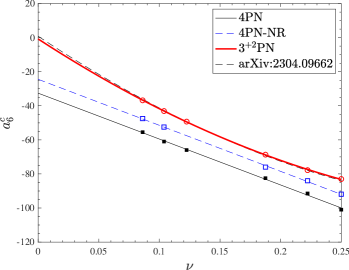
Figure 2: Behavior of $a_{6}^{c}$ for different approximations to the $\rho_{22}$ function. The 4PN-accurate function (in Padé-resummed form) entails values of $a_{6}^{c}$ that are smaller than the case with $\rho_{22}$ at $3^{+2}$ PN accuracy in Taylor-expanded form. This mirrors a more attractive conservative dynamics (the radius of the LSO is larger, see Table 2) that compensates for the weaker action of radiation reaction due to $P^{2}_{2}(\rho_{22}^{\rm 4PN})<\rho_{22}^{\rm 3^{+2}PN}$, as shown in Fig. 1. The 4PN-NR line, that lies between the other two, refers to the case where the analytical $\nu$-dependence in the 4PN is replaced by a suitably NR-informed one, consistently with Fig. 9 below. See text for additional details.

Table 1: Data used to NR-inform the nonspinning section of the model(s) with various choices for radiation reaction. From left to right: the Taylor-expanded $\rho_{22}$ function at $3^{+2}$ PN accuracy; the $(2,2$) Padé-resummed $\rho_{22}$ function at 4PN accuracy; the (2,2) Padé resummed $\rho_{22}$ at formal 4PN accuracy with the NR-informed $\nu$-dependence of the 4PN coefficient $c_{4}$. The corresponding values of $c_{4}^{\nu}$ are listed in the last column of the table. The fits of the various $a_{6}^{c}$ points are illustrated in Fig. 2.

$\#$	ID	$q$	$a_{6}^{c,3^{+2}\rm PN}$	$a_{6}^{\rm c,4PN}$	$a_{6}^{\rm c,4PN-NR}$	$c_{4}^{\nu}$
1	SXS:BBH:0180	$1$	$-83$	$-101$	$-91.9$	$-13.5$
2	SXS:BBH:0169	$2$	$-77.8$	$-91.5$	$-84$	$-11.4$
3	SXS:BBH:0168	$3$	$-68.7$	$-82.5$	$-76$	$-8.5$
4	SXS:BBH:0166	$6$	$-49.3$	$-66$	$\dots$	$\dots$
5	SXS:BBH:0299	$7.5$	$-43.1$	$-61$	$-52.5$	$-2.5$
6	SXS:BBH:0302	$9.5$	$-36.8$	$-55.5$	$-47.5$	$-1.1$

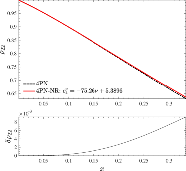
Figure 9: Informing an effective 4PN term $c_{4}^{\nu}$ in $\rho_{22}$ using NR data, Eq. (41) in the equal-mass case. The bottom panel shows the relative difference normalized to the 4PN analytic curve, $\delta\rho_{22}$, that is  $0.6\%$ at $x_{\rm LSO}\sim 0.25$ (see Table 2). Such a (tiny) difference is actually necessary to lower the EOB/NR unfaithfulness by approximately one order of magnitude, up to $\sim 10^{-4}$, see Fig. 10.

Table 2: Properties of the last stable orbit (LSO) obtained with the NR-informed $a_{6}^{c}$ using $\rho_{22}^{3^{\rm+2PN}}$ or $P^{2}_{2}(\rho_{22}^{\rm 4PN})$ with the analytical or the NR-informed 4PN coefficient (4PN-NR case). Lowering $a_{6}^{c}$ as is needed when using $P^{2}_{2}(\rho_{22}^{\rm 4PN})$ entails a larger value of $r_{\rm LSO}$ and thus a faster plunge, so to compensate that $P^{2}_{2}(\rho_{22}^{\rm 4PN})<\rho_{22}^{\rm 3^{+2}PN}$ during the late inspiral as shown in Fig. 1. The 4PN-NR value is similarly understood by comparing with the NR-tuned $P^{2}_{2}(\rho_{22}^{\rm 4PN})$ in Fig. 9.

model	$p_{\varphi}^{\rm LSO}$	$r_{\rm LSO}$	$u_{\rm LSO}$
$3^{+2}$PN	3.034	2.72	0.367
$4$PN	3.191	4.092	0.244
4PN-NR	3.167	3.631	0.275
TEOBResumS-Giotto	3.225	4.517	0.221
Schwarzschild	3.464	6.0	$0.1\bar{6}$

In the nonspinning case, Ref. [13] first introduced the model using the $\rho_{22}^{3^{+2}\rm PN}$ waveform and radiation reaction. Its performance was evaluated in the quasi-circular, eccentric and scattering case, with explicit comparisons of the scattering angle (see Figs. 12 and  14 as well as Table III therein). To start with, we need then to compare the performance of this model with the new one obtained using the 4PN-resummed radiation reaction (and a newly determined $a_{6}^{c}$). While doing so, we realized the presence of a small bug in the implementation of $F_{r}$ in Ref. [13]. Although this has minimal quantitative effects, we redo here the full analysis of Sec. IV of Ref. [13], while also NR-completing the 4PN-resummed model. To start with, we determine $a_{6}^{c}$ by EOB/NR phasing comparisons, with the requirement, clearly pointed out in [13], that the EOB/NR phase difference grows monotonically, so to have the smallest values of the EOB/NR unfaithfulness. To inform $a_{6}^{c}$ we use only six NR datasets, that are listed in Table 1. The points are visualized in Fig. 2 They are easily representable by the following fits. For $\rho_{22}$ at $3^{+2}$ PN accuracy the values are consistent with those of Ref. [13] and can be fitted with a quadratic function

$$a_{6}^{c,{\rm 3^{+2}PN}}=530.9514\nu^{2}-462.5404\nu-0.78979\ .$$ (33)

For $P^{2}_{2}(\rho_{22}^{\rm 4PN})$, the functional behavior of the $a_{6}^{c}$ points is simpler, as they can be accurately fitted by the following linear regression

$$a_{6}^{c,{\rm 4PN}}=-32.5953-269.4331\nu\ .$$ (34)

The fact that for the 4PN case $a_{6}^{c}$ is always smaller than for the $3^{+2}$PN case is the consequence of $P^{2}_{2}(\rho_{22}^{\rm 4PN})<\rho_{22}^{\rm 3^{+2}PN}$. From the physical point of view, this follows from the fact that the radiation reaction (i.e., mainly the flux of angular momentum) is smaller in one case than in the other. As a result, to have the EOB waveform NR faithful one must tune the conservative dynamics (through $a_{6}^{c}$) so as to compensate this effect. In practice, as we will see below, lowering the value of $a_{6}^{c}$ means increasing the value of $r_{\rm LSO}$, which prompts a faster transition from the radiation-reaction driven inspiral to plunge. In Figure 3 we show four illustrative EOB/NR phasings for $q=1$ and $q=8$ obtained with either the $3^{+2}$ PN prescription (left-panels) or the 4PN prescription (right panels). Note that the EOB/NR phase difference is (essentially) monotonic in both cases, but its sign is different.

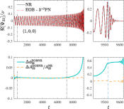
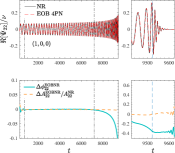
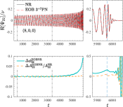
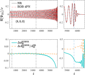
Figure 3: Left panels: EOB/NR phasings obtained with $\rho_{22}^{3^{+2}\rm PN}$ and $a_{6}^{c}$ given by Eq. (33). Right panels: EOB/NR phasings obtained with $\rho_{22}^{4\rm PN}$ and $a_{6}^{c}$ given by Eq. (34).

The corresponding values of the LSO for $q=1$ are listed in Table 2. One sees that the fact that the lowering of $a_{6}^{c}$ needed when using $P^{2}_{2}(\rho_{22}^{\rm 4PN})$ entails a larger value of $r_{\rm LSO}$ and thus a faster plunge, so to compensate for $P^{2}_{2}(\rho_{22}^{\rm 4PN})<\rho_{22}^{\rm 3^{+2}PN}$ during the late inspiral. On top of this, it is remarkable to note that when $\rho_{22}^{\rm 3^{+2}PN}$ is used, the good, NR-informed, value of the LSO is rather small, $r_{\rm LSO}=2.72$, notably a $25\%$ smaller than the value for $P^{2}_{2}(\rho_{22}^{\rm 4PN})$. This is needed to compensate for what seems to be an incorrectly large radiation reaction during the inspiral. With this vision in mind, one can better understand the left panels of Fig. 3 and in particular the meaning of the fact that the phase difference $\Delta\phi^{\rm EOBNR}_{22}\equiv\phi^{\rm EOB}_{22}-\phi^{\rm NR}_{22}$ is positive: the radiation-reaction-dominated inspiral progresses faster than the NR one, so that $\phi_{22}^{\rm EOB}>\phi_{22}^{\rm NR}$ and thus $\Delta\phi^{\rm EOBNR}_{22}>0$. This effect is compensated by the repulsive character of the EOB dynamics that is magnified by tuning $a_{6}^{c}$ so that the LSO occurs at a rather small value of $r$. With the same rationale in mind, it is similarly easy to interpret the right panels of Fig. 3, that exhibit a negative phase difference that begins to grow already during the late inspiral. This indicates that the effect of radiation reaction (mainly related to the amplitude of $\rho_{22}$ being too small) is insufficient (with respect to the NR benchmark) and thus the transition from inspiral to plunge, merger and ringdown is delayed with respect to the NR case.

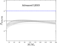
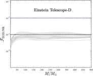
Figure 4: EOB/NR unfaithfulness for the $\ell=m=2$ mode in the nonspinning case for mass ratios $1\leq q\leq 10$ using the 4PN-accurate (resummed) $\rho_{22}$ function.The performance is similar, though slightly better, to the one obtained for $\rho_{22}$ in Taylor-expanded form at $3^{+2}$ PN accuracy, Fig. 12 in Ref. [13].

The quantitative assessment of the quality of our new EOB model is finally completed by computing the EOB/NR unfaithfulness. Since this quantity was computed in Ref. [13] using the $3^{+2}$ PN expression of $\rho_{22}$, it is also pedagogically useful to compute it here with the 4PN-resummed model. Figure 4 reports the values of $\bar{{\cal F}}$ for a sample of nonspinning binaries with $1\leq q\leq 10$ stepped by 0.5. The performance of the 4PN model is substantially comparable to that of the $3^{+2}$ PN one, although one has a small gain for high masses (cf. Fig. 12 in [13]). With this so well under control, we are ready to move to discussing the spin sector of the model.

III.2 Spin-aligned and EOB/NR performance in the quasi-circular case

Table 3: Coefficients for the fit of $c_{3}$ given by Eq. (35) for the two NR-informed model discussed in the main text. The Dali_4PN-analytic one incorporates the 4PN information in the nonspinning $\rho_{22}^{\rm orb}$ function; in the Dali_4PN-NRTuned model the same term is instead informed using nonspinning NR waveforms.

Model	$c_{3}^{=}\equiv p_{0}\left(1+n_{1}\tilde{a}_{0}+n_{2}\tilde{a}_{0}^{2}+n_{3}\tilde{a}_{0}^{3}+n_{4}\tilde{a}_{0}^{4}\right)/\left(1+d_{1}\tilde{a}_{0}\right)$
	$c_{3}^{\neq}\equiv\left(p_{1}\tilde{a}_{0}+p_{2}\tilde{a}_{0}^{2}+p_{3}\tilde{a}_{0}^{3}\right)\sqrt{1-4\nu}+p_{4}\tilde{a}_{0}\nu\sqrt{1-4\nu}+\left(p_{5}\tilde{a}_{12}+p_{6}\tilde{a}_{12}^{2}\right)\nu^{2}$
TEOBResumS*	$p_{0}$	$n_{1}$	$n_{2}$	$n_{3}$	$n_{4}$	$d_{1}$	$p_{1}$	$p_{2}$	$p_{3}$	$p_{4}$	$p_{5}$	$p_{6}$
Dali4PN-analytic	38.625	$-0.105187$	$-0.758427$	$0.183613$	$0.057817$	$0.905420$	$23.058$	$12.544$	$-0.0157$	$-119.2596$	$64.4709$	$54.6568$
Dali4PN-NRTuned	44.616	$-1.609364$	0.807277	$-0.220357$	$0.045408$	$-0.7704$	5.67453	$-1.214$	12.3433	$-16.5925$	$-0.7784$	$-55.1691$

To complete the spin sector, we need to NR-inform the N³LO effective spin-orbit parameter $c_{3}$ introduced above (see [32]). This procedure was already implemented in previous versions of the TEOBResumS-Dalí model [7, 10], but it was always found complicated to reduce the EOB/NR unfaithfulness for large, positive, values of the spins, as discussed extensively in Ref. [10]. We find that the new analytical setup finally allows us to overcome this problem. The NR-informed analytical expression for $c_{3}$ is obtained using the same functional form and the same set of SXS NR data of Ref. [13]. It reads:

$$c_{3}(\nu,\tilde{a}_{0},\tilde{a}_{12})=c^{=}_{3}+c_{3}^{\neq}\ ,$$ (35)

where

$$c_{3}^{=} \equiv p_{0}\dfrac{1+n_{1}\tilde{a}_{0}+n_{2}\tilde{a}_{0}^{2}+n_{3}\tilde{a}_{0}^{3}+n_{4}\tilde{a}_{0}^{4}}{1+d_{1}\tilde{a}_{0}}$$ (36)

$$c_{3}^{\neq} \equiv\left(p_{1}\tilde{a}_{0}+p_{2}\tilde{a}_{0}^{2}+p_{3}\tilde{a}_{0}^{3}\right)\sqrt{1-4\nu}$$

$$+p_{4}\tilde{a}_{0}\nu\sqrt{1-4\nu}+\left(p_{5}\tilde{a}_{12}+p_{6}\tilde{a}_{12}^{2}\right)\nu^{2}\ ,$$ (37)

The NR configurations we used to inform $c_{3}$ are listed in Tables 8-9 in Appendix C. For each configuration, we determine the best-guess value of $c_{3}$ via time-domain phasing comparison. Then, the resulting values are fitted using the above functional form. The coefficients of the fit are reported in Table 3. Since this model relies on 4PN analytical information, we will refer to it as ${\tt TEOBResumS-Dali_{4PN-analytic}}$ or just Dali_4PN-analytic for simplicity.

We focus first on the $\ell=m=2$ waveform mode and estimate the EOB/NR unfaithfulness $\bar{{\cal F}}_{\rm EOBNR}$ with the Advanced LIGO PSD.

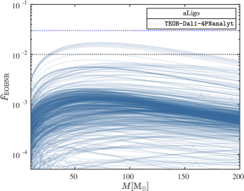
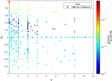
Figure 5: EOB/NR unfaithfulness for the $\ell=m=2$ mode. The performance of the model gets progressively worst in the equal-mass, high-spin corner. This is consistent with a previous version of the model, but less pronounced.

Figure 5 shows $\bar{{\cal F}}_{\rm EOBNR}$ computed all over the 534 spin-aligned datasets of the SXS catalog. The left panel of the figure shows $\bar{{\cal F}}_{\rm EOBNR}$ versus the total mass, while the right panel the maximum value for each configurations, $\bar{{\cal F}}^{\rm max}_{\rm EOBNR}$. We see that the unfaithfulness always lies below the $1\%$ threshold except for a few outliers in the equal-mass, high (positive) spin corner, that in any case do not exceed the $2\%$ level. This result alone represents an improvement with respect to previous work [7]. It is also useful to provide a direct comparison with waveforms generated with the NR surrogates NRHybSur3dq8 [46] and NRHybSur2dq15 [47]. We generate 1000 randomly sampled configurations with $q\in[1,8]$, total mass $M\in[40,140]M_{\odot}$ and dimensionless spins $|\chi_{i}|<0.8$ and compute mismatches in the frequency interval between $[20,2048]$ Hz. Similarly, when working with NRHybSur2dq15, we consider another 1000 randomly sampled configurations with $q\in[8,15]$, and dimensionless spins $|\chi_{1}|\leq 0.5$, $\chi_{2}=0$, corresponding to the validity range of the surrogate model. The values of $\bar{{\cal F}}$ are reported in Fig. 6, together with those corresponding to the quasi-circular version of the model, TEOBResumS-GIOTTO, calculated in Ref. [10].

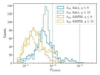
Figure 6: EOB/NR unfaithfulness for the $\ell=m=2$ model against the NR surrogate NRHybSur3dq8 and NRHybSur2dq15. In the first case, $q\in[1,8]$, $M\in[40,140]M_{\odot}$ and dimensionless spins are $|\chi_{i}|<0.8$. In the second case $q\in[8,15]$, $|\chi_{1}|\leq 0.5$ and $\chi_{2}=0$

The figure clearly indicates that the quasi-circular limit of Dali_4PN-analytic is acceptably consistent with the behavior of the basic quasi-circular model. We remind the reader that this, a priori, is not a trivial achievement because of the many theoretical differences between the two models. We are now expecting that this new version of Dali_4PN-analytic will allow us to reduce (or eliminate) the systematics in parameter estimation that were found using previous versions of the model [4].

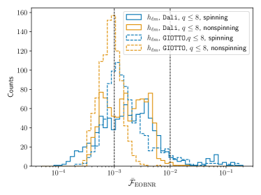
Figure 7: EOB/NR unfaithfulness for the higher modes, for the same configurations considered in Fig. 6.

Table 4: SXS simulations with eccentricity analyzed in this work. From left to right: the ID of the simulation from the SXS catalog; the mass ratio $q\equiv m_{1}/m_{2}\geq 1$ and the individual dimensionless spins $(\chi_{1},\chi_{2})$; the time-domain NR phasing uncertainty at merger $\delta\phi^{\rm NR}_{\rm mrg}$ obtained comparing the highest and second highest resolution; the estimated NR eccentricity at first apastron $e_{\omega_{a}}^{\rm NR}$; the NR frequency of first apastron $\omega_{a}^{\rm NR}$; the initial EOB eccentricity $e^{\rm EOB}_{\omega_{a}}$ and apastron frequency $\omega_{a}^{\rm EOB}$ used to start the EOB evolution; the maximal NR unfaithfulness uncertainty, $\bar{{\cal F}}^{\rm max}_{\rm NRNR}$ and the initial frequency $Mf_{\rm min}$ used in the EOB/NR unfaithfulness computation shown in Figs. 8 using the 4PN analytical information in the flux and in Fig. 12 using the corresponding NR-tuned one. The last two columns report the corresponding maximum values of $\bar{{\cal F}}_{\rm EOBNR}^{\rm max}$, the analytical, $\bar{{\cal F}}_{\rm EOBNR}^{\rm max,4PNan}$, and the NR-tuned one, $\bar{{\cal F}}_{\rm EOBNR}^{\rm max,4PNnr}$.

$\#$	id	$(q,\chi_{1},\chi_{2})$	$\delta\phi^{\rm NR}_{\rm mrg}$[rad]	$e^{\rm NR}_{\omega_{a}}$	$\omega_{a}^{\rm NR}$	$e^{\rm EOB}_{\omega_{a}}$	$\omega_{a}^{\rm EOB}$	$\bar{{\cal F}}_{\rm NRNR}^{\rm max}[\%]$	$Mf_{\rm min}$	$\bar{{\cal F}}_{\rm EOBNR}^{\rm max,4PNan}$	$\bar{{\cal F}}_{\rm EOBNR}^{\rm max,4PNnr}$
1	BBH:1355	$(1,0,0)$	$+0.92$	0.0620	0.03278728	0.0888	0.02805750	0.012	0.0055	0.173	0.026
2	BBH:1356	$(1,0,0)$	$+0.95$	0.1000	0.02482006	0.15038	0.019077	0.0077	0.0044	0.159	0.052
3	BBH:1358	$(1,0,0)$	$+0.25$	0.1023	0.03108936	0.18082	0.021238	0.016	0.0061	0.328	0.065
4	BBH:1359	$(1,0,0)$	$+0.25$	0.1125	0.03708305	0.18240	0.021387	0.0024	0.0065	0.441	0.327
5	BBH:1357	$(1,0,0)$	$-0.44$	0.1096	0.03990101	0.19201	0.01960	0.028	0.0061	0.198	0.101
6	BBH:1361	$(1,0,0)$	+0.39	0.1634	0.03269520	0.23557	0.020991	0.057	0.0065	0.357	0.113
7	BBH:1360	$(1,0,0)$	$-0.22$	0.1604	0.03138220	0.2440	0.019508	0.0094	0.0065	0.254	0.085
8	BBH:1362	$(1,0,0)$	$-0.09$	0.1999	0.05624375	0.3019	0.01914	0.0098	0.0065	0.244	0.119
9	BBH:1363	$(1,0,0)$	$+0.58$	0.2048	0.05778104	0.30479	0.01908	0.07	0.006	0.520	0.381
10	BBH:1364	$(2,0,0)$	$-0.91$	0.0518	0.03265995	0.0844	0.025231	0.049	0.062	0.089	0.054
11	BBH:1365	$(2,0,0)$	$-0.90$	0.0650	0.03305974	0.110	0.023987	0.027	0.062	0.109	0.073
12	BBH:1366	$(2,0,0)$	$-6\times 10^{-4}$	0.1109	0.03089493	0.14989	0.02577	0.017	0.0052	0.201	0.148
13	BBH:1367	$(2,0,0)$	$+0.60$	0.1102	0.02975257	0.15095	0.0260	0.0076	0.0055	0.108	0.095
14	BBH:1368	$(2,0,0)$	$-0.71$	0.1043	0.02930360	0.14951	0.02512	0.026	0.0065	0.169	0.201
15	BBH:1369	$(2,0,0)$	$-0.06$	0.2053	0.04263738	0.3134	0.0173386	0.011	0.0041	0.559	0.560
16	BBH:1370	$(2,0,0)$	$+0.12$	0.1854	0.02422231	0.31708	0.016779	0.07	0.006	0.430	0.217
17	BBH:1371	$(3,0,0)$	$+0.92$	0.0628	0.03263026	0.0912	0.029058	0.12	0.006	0.179	0.115
18	BBH:1372	$(3,0,0)$	$+0.01$	0.1035	0.03273944	0.14915	0.026070	0.06	0.006	0.105	0.060
19	BBH:1373	$(3,0,0)$	$-0.41$	0.1028	0.03666911	0.15035	0.02529	0.0034	0.0061	0.749	0.705
20	BBH:1374	$(3,0,0)$	$+0.98$	0.1956	0.02702594	0.314	0.016938	0.067	0.0059	0.473	0.385
21	BBH:89	$(1,-0.50,0)$	$\dots$	0.0469	0.02516870	0.07194	0.01779	$\dots$	0.0025	0.214	0.0749
22	BBH:1136	$(1,-0.75,-0.75)$	$-1.90$	0.0777	0.04288969	0.1209	0.02728	0.074	0.0058	0.356	0.152
23	BBH:321	$(1.22,+0.33,-0.44)$	$+1.47$	0.0527	0.03239001	0.07621	0.02694	0.015	0.0045	0.204	0.033
24	BBH:322	$(1.22,+0.33,-0.44)$	$-2.02$	0.0658	0.03396319	0.0984	0.026895	0.016	0.0061	0.203	0.0486
25	BBH:323	$(1.22,+0.33,-0.44)$	$-1.41$	0.1033	0.03498377	0.1438	0.02584	0.019	0.0058	0.131	0.0745
26	BBH:324	$(1.22,+0.33,-0.44)$	$-0.04$	0.2018	0.02464165	0.29425	0.01894	0.098	0.0058	1.209	0.671
27	BBH:1149	$(3,+0.70,+0.60)$	$+3.00$	0.0371	0.03535964	$0.06237$	$0.02664$	0.025	0.005	0.660	1.166
28	BBH:1169	$(3,-0.70,-0.60)$	$+3.01$	0.0364	0.02759632	$0.04895$	$0.024285$	0.033	0.004	0.178	0.129

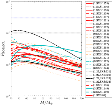
Figure 8: EOB/NR unfaithfulness for the $\ell=m=2$ mode computed over the 28 eccentric inspiral SXS simulations publicly available of Table 4. The horizontal lines mark the $0.03$ and $0.01$ values. $\bar{{\cal F}}^{\rm max}_{\rm EOBNR}$ is always below $0.01$, although the performance slightly degrades for large, positive, spins, consistently with the quasi-circular limit behavior.

III.2.1 Higher waveform multipoles

Although the main focus of this work lies in the examination of the quadrupolar $(\ell,|m|)=(2,2)$ mode, TEOBResumS can be employed to generate waveforms encompassing higher modes as well. In the realm of inspiral-to-merger-only waveforms, the model can compute waveforms containing modes up to $\ell=m=8$, while the complete merger-ringdown (IMR) phase is accessible for $(2,|1|),(3,|3|),$ and $(4,|4|)$ modes, utilizing the fits described in [48, 13]. See in particular Ref. [13] for a description of the modifications needed within the TEOBResumS framework to use the NR-informed ringdown fits of Ref. [48]. The careful reader will notice that the full content of IMR higher modes in this version of TEOBResumS is comparatively lower than its quasi-circular counterpart, TEOBResumS-GIOTTO [13]. This discrepancy arises from the intricacies of modeling binaries on non-circularized orbits, where the conventional strategy employed for transitioning between inspiral-plunge and merger phases faces challenges. EOB models designed for quasi-circular orbits incorporate next-to-quasi-circular NR-informed corrections (NQCs) in the waveform. These corrections account for non-circular effects during plunge, ensuring a seamless connection between pre- and post-merger waveforms. In contrast, when the binary system is non-circularized from the outset, this conventional strategy must be reevaluated. Reference [7] introduced a sigmoid function to smoothly eliminate the non-circular Newtonian prefactor, that might become inaccurate close to merger, and progressively activate the NR-informed NQCs. While this method has proven simply effective for the $(2,2)$ mode, for higher modes its interplay with the so-called NQC basis might generate inaccuracies around the waveform peak in some regions of the parameter space. While an in-depth characterization of these effects lies beyond the scope of this work here we present a preliminary, simple improvement to the $(2,1)$ mode that allows us to increase the NR faithfulness of the multipolar model. Let us briefly review some basic information about NQC corrections within the present context. We address the reader to Sec. IIB of Ref. [7]. The EOB multipolar NQC corrections to the waveform are formally given by

$$\hat{h}_{\ell m}^{\rm NQC}=\left(1+a_{1}^{\ell m}n_{1}^{\ell m}+a_{2}^{\ell m}n_{2}^{\ell m}\right)e^{i(b_{1}^{\ell m}n_{3}^{\ell m}+b_{2}^{\ell m}n_{4}^{\ell m})}\ ,$$ (38)

where $\{a_{i}^{\ell m},b_{i}^{\ell m}\}$ are coefficients determined following the procedure detailed in e.g. Ref. [8], and $\{n_{1}^{\ell m},\dots,n_{4}^{\ell m}\}$ are functions depending on the EOB dynamical variables. Similar to other EOB building blocks, there is some freedom in choosing these functions, given their effective nature. So far, the choice of $n_{i}$’s implemented in the Dalí model differs slightly from those used in the GIOTTO model and is the one detailed at the end of Sec. IIB of Ref. [7]. Using these functions, we find that for some configurations, characterized by large, positive spins, the NQC correction to the frequency evolution presents an unphysical repentine increase during the late inspiral. We find that this unwanted behavior is easily cured by using the following $n_{4}$ function

$$n_{4}^{21}=r\Omega p_{r_{*}}\ ,$$ (39)

instead of $p_{r_{*}}/(r\Omega^{1/3})$ previously implemented. This simple modification allows us to obtain a more correct frequency evolution for the considered mode.

After performing this improvement, we compute the EOB/NR surrogate unfaithfulness considering higher modes for the same configurations considered in Fig. 6. Following the same procedure as Ref. [13], we fix the inclination angle to $\iota=\pi/3$ and minimize the unfaithfulness over the sky-position of the binary. Results are shown in Fig. 7. The EOB/NR unfaithfulness obtained with the generic-orbits model is overall consistent with the one computed with the quasi-circular model, though characterized by longer tails towards larger values of mismatch. Such tails can reach up to $\sim 10\%$ for binaries with large, positive spins, although the model is NR faithful to more than $1\%$ for a large portion of the parameter space.

Table 5: Comparison between EOB and NR scattering angle for nonspinning binaries using either $\rho_{22}^{\rm 3^{+2}PN}$ , the resummed (analytical) $\rho_{22}^{\rm 4PN}$ or the NR-tuned one. The NR values are taken from the nonspinning configurations from Ref. [41] and Ref. [11].

$\#$	$r^{3^{+2}\rm PN}_{\rm min}$	$r^{4\rm PNan}_{\rm min}$	$r^{4\rm PNnr}_{\rm min}$	$E_{\rm in}^{\rm NR}/M$	$J_{\rm in}^{\rm NR}/M^{2}$	$\chi^{\rm NR}$	$\chi^{\rm EOB}_{3^{+2}\rm PN}$	$\chi^{\rm EOB}_{\rm 4PN-Analytic}$	$\chi^{\rm EOB}_{\rm 4PN-NRTuned}$	$[\%]$	$[\%]$	$[\%]$
1	3.430	3.375	3.408	1.0225555(50)	1.099652(36)	305.8(2.6)	315.94	346.83	326.79	3.31	13.42	6.86
2	3.760	3.738	3.751	1.0225722(50)	1.122598(37)	253.0(1.4)	258.54	265.87	261.06	2.19	5.09	3.18
3	4.059	4.050	4.057	1.0225791(50)	1.145523(38)	222.9(1.7)	225.25	227.85	225.95	1.05	2.22	1.37
4	4.862	4.862	4.863	1.0225870(50)	1.214273(40)	172.0(1.4)	171.62	171.77	171.51	0.22	0.13	0.28
5	5.352	5.353	5.353	1.0225884(50)	1.260098(41)	152.0(1.3)	151.31	151.27	151.18	0.45	0.48	0.54
6	6.503	6.504	6.504	1.0225907(50)	1.374658(45)	120.7(1.5)	119.99	119.92	119.92	0.58	0.64	0.64
7	7.601	7.602	7.602	1.0225924(50)	1.489217(48)	101.6(1.7)	101.09	101.05	101.05	0.49	0.54	0.53
8	8.675	8.675	8.675	1.0225931(50)	1.603774(52)	88.3(1.8)	87.98	87.95	87.96	0.36	0.39	0.39
9	9.735	9.735	9.735	1.0225938(50)	1.718331(55)	78.4(1.8)	78.18	78.16	78.16	0.28	0.30	0.30
10	10.788	10.789	10.788	1.0225932(50)	1.832883(58)	70.7(1.9)	70.50	70.49	70.49	0.28	0.30	0.29
11	3.02	$\dots$	2.97	1.035031(27)	1.1515366(78)	307.13(88)	338.0382	plunge	393.73	10.06	$\dots$	$28.2$
12	3.91	3.90	3.91	1.024959(12)	1.151845(12)	225.54(87)	230.0844	234.04	231.37	2.01	3.77	2.58
13	4.41	4.41	4.41	1.0198847(82)	1.151895(11)	207.03(99)	207.5565	208.43	207.6076	0.26	0.68	0.28
14	4.99	4.99	4.99	1.0147923(76)	1.151918(16)	195.9(1.3)	194.6248	194.6735	194.4233	0.67	0.64	0.77
15	6.68	6.68	6.68	1.0045678(42)	1.1520071(73)	201.9(4.8)	200.1620	199.9873	200.0012	0.87	0.95	0.94

Table 6: Comparison between EOB and the (average) NR scattering angle for some of the equal-mass, spin-aligned, configurations of Ref. [42]. All datasets share the same initial angular momentum $J_{\rm in}^{\rm NR}/M^{2}=1.14560$. The EOB angles are calculated either using the (resummed) analytical $\rho_{22}^{\rm 4PN}$ or the effective 4PN NR-tuned one, with the corresponding values of $a_{6}^{c}$ and $c_{3}$. Note that for large values of the (anti)-aligned spins the EOB dynamics plunges instead of scattering.

$\chi_{1}$	$\chi_{2}$	$\tilde{a}_{0}$	$E_{\rm in}^{\rm NR}/M$	$r^{4\rm PNan}_{\rm min}$	$r^{4\rm PNnr}_{\rm min}$	$\chi^{\rm NR}$	$\chi^{\rm EOB}_{\rm 4PN-Analytic}$	$\chi^{\rm EOB}_{\rm 4PN-NRTuned}$	$\Delta\chi_{\rm 4PNan}^{\rm EOBNR}[\%]$	$\Delta\chi_{\rm 4PNnr}^{\rm EOBNR}[\%]$
$-0.3$	$-0.30$	$-0.30$	1.022690	$\dots$	$\dots$	$plunge$	$plunge$	$plunge$	$\dots$	$\dots$
$-0.25$	$-0.25$	$-0.25$	1.022680	$\dots$	$\dots$	367.55	$plunge$	$plunge$	$\dots$	$\dots$
$-0.23$	$-0.23$	$-0.23$	1.022670	$\dots$	$\dots$	334.35	$plunge$	$plunge$	$\dots$	$\dots$
$-0.20$	$-0.20$	$-0.20$	1.022660	$3.46$	3.50	303.88	386.9102	352.5517	27.32	16.02
$-0.15$	$-0.15$	$-0.15$	1.022650	$3.65$	3.68	272.60	305.6974	294.9987	12.14	8.22
$-0.10$	$-0.10$	$-0.10$	1.022650	$3.80$	3.82	251.03	269.0546	263.6445	7.18	5.03
$-0.05$	$-0.05$	$-0.05$	1.022640	$3.93$	3.94	234.57	245.3143	242.1832	4.58	3.25
$+0.00$	$0.0$	$0.0$	1.022640	$4.04$	4.05	221.82	228.1024	226.1822	2.83	1.97
$+0.10$	$+0.10$	$+0.10$	1.022650	$4.24$	4.24	202.61	203.7849	203.0811	0.58	0.23
$+0.20$	$+0.20$	$+0.20$	1.022660	$4.40$	4.40	187.84	186.8409	186.7207	0.53	0.59
$+0.20$	$-0.20$	$0.0$	1.022660	$4.04$	4.05	221.82	228.1338	226.2067	2.85	1.98
$+0.30$	$+0.30$	$+0.30$	1.022690	$4.53$	4.53	176.59	174.0689	174.2778	1.43	1.31
$+0.40$	$+0.40$	$+0.40$	1.022740	$4.65$	4.65	167.54	163.9378	164.3545	2.15	1.90
$+0.60$	$+0.60$	$+0.60$	1.022880	$4.85$	4.84	154.14	148.6040	149.3273	3.59	3.12
$+0.60$	$0.0$	$+0.30$	1.022760	$4.53$	4.53	177.63	174.2648	174.2686	1.89	1.89
$+0.70$	$-0.30$	$+0.20$	1.022840	$4.38$	4.38	190.41	187.2741	186.7755	1.65	1.91
$+0.80$	$-0.80$	$0.0$	1.023090	$4.01$	4.02	221.68	229.5845	227.4832	3.57	2.62
$+0.80$	$-0.50$	$+0.15$	1.022940	$4.30$	4.30	198.99	195.3268	194.4505	1.84	2.28
$+0.80$	$+0.20$	$+0.50$	1.022880	$4.75$	4.75	162.07	155.7832	156.1319	3.88	3.66
$+0.80$	$+0.50$	$+0.65$	1.022950	$4.89$	4.88	152.30	145.5650	146.3084	4.42	3.94
$+0.80$	$+0.80$	$+0.80$	1.023090	$5.00$	4.99	145.36	137.3641	139.1984	5.50	4.24

III.3 Eccentric inspirals

Let us now consider the performance of the model for mildly eccentricy bound systems. Figure 8 shows the EOB/NR unfaithfulness versus $M$ computed with the 28 SXS simulations of eccentric inspirals currently publicly available [40]. In spite of these datasets being rather old, to date these remain the only SXS data available for non-circular orbits spanning a considerable number of orbits. Other eccentric NR waveforms do exist, e.g. from the RIT [49] and MAYA catalogs [50], but are typically shorter. The properties of the datasets considered are collected in Table 4. Following previous works, when performing EOB/NR comparisons it is necessary to tune two parameters – the initial frequency at apastron $\omega_{0}$ and initial nominal eccentricity $e_{0}$ – to correctly match the EOB and NR inspirals. This is required, in our case, because for simplicity the EOB dynamics is always started at apastron, with zero initial radial momentum. This choice is consistent with previous works of this lineage, from the very first development of an eccentric model within the TEOBResumS framework [2]. Notably, similar coverage of the parameter space can be obtained by fixing the initial frequency, and allowing the initial (true or mean) anomaly to vary. This is, for example, the choice made in Ref. [20]. As also pointed out in this reference, (i) starting the eccentric inspiral at the apastron and varying on initial frequency and eccentricity is equivalent to (ii) starting the eccentric inspiral at fixed initial frequency and varying on eccentricity and anomaly. Both choices entail a complete coverage of the parameter space, though the approach (ii) is intuitively closer to what usually done for quasi-circular binaries. In Appendix B we discus the implementation of the anomaly and a description of initial data that is close, though different, to the one of Ref. [20]. However, for consistency with previous work, we here keep giving initial data at apastron. Figure 8 shows the EOB/NR unfaithfulness versus $M$. The results improve with respect to previous work, with $\bar{{\cal F}}^{\rm EOBNR}\lesssim 1\%$ all over the dataset sample. The plot is complemented by Tab. 4.

III.4 Scattering configurations

We conclude this section by considering unbound configurations, and in particular BBH scatterings. Rather than computing and comparing waveforms, a non-trivial feat from the NR side, we directly gauge the goodness of the EOB dynamics by performing comparisons of the gauge-invariant EOB and NR scattering angles. Following standard procedures already adopted in previous work, we consider the nonspinning configurations of Refs. [41, 11] (see Tab. 5) and the spinning configurations of Ref. [42] (see in Tab. 6). We do not perform detailed comparisons for the spinning simulations presented in Ref. [11] because they are limited to rather extreme cases, with large energies and spins, and do not present a systematic and detailed analysis of the numerical error, which was instead performed in Ref. [42]. Collectively, these result suggest that the analytical EOB description for spin-aligned binaries becomes less accurate in the part of the parameter space that is close to the capture threshold. This is evident for the data of Ref. [42] listed in Table 6, where we can see the sequence as the effective spin $\tilde{a}_{0}$ is decreased, but the same phenomenology is present also in the data of Ref. [11], although they were not such to systematically cover the transition.

Let us finally mention that, for the nonspinning configurations of Table 5, we also list EOB calculations that use the model based on $3^{+2}$ PN Taylor-expanded $\rho_{22}$ function. For the most extreme configurations (first rows in Table 5) the corresponding angles are closer to the NR ones than those obtained using the fully analytical 4PN $\rho_{22}$. The fact that a model that is less NR-faithful for quasi-circular configurations is actually more NR-faithful for scattering configurations highlights the difficulty in constructing a model capable of covering well all configurations, as well as the delicate interplay between dissipative and conservative effect in the description of the dynamics. In the next section we will see that it is actually possible to do better by carefully improving the description of the radiation reaction using NR information. The delicacy of the interplay between the various effects is evident by looking at dataset number 11 in Table 5: in the $3^{+2}$ PN case we have a scattering (that is, at least, qualitatively consistent with the NR prediction) while in the 4PN case the system plunges.

IV Noncircularized waveform model with NR-informed radiation reaction

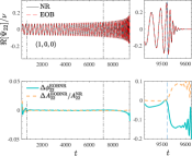
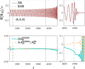
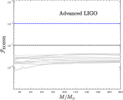
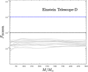
Figure 10: Nonspinning case: NR-informing at the same time the EOB interaction potential (via $a_{6}^{c}$, Eq. (40)) and the resummed radiation reaction via $c_{4}^{\nu}$, Eq. (41). Top panels: two illustrative time-domain phasings. Bottom panels: EOB/NR unfaithfulness for all SXS nonspinning datasets available (up to $q=15$) with both the Advanded-LIGO and ET-D sensitivity designs. Phase differences accumulated at merger $\lesssim 0.1$ rad yield $\bar{{\cal F}}_{\rm EOBNR}\sim 10^{-4}$.

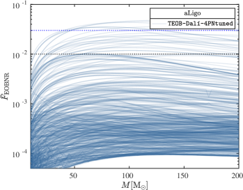
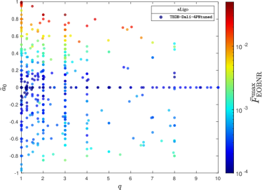
Figure 11: EOB/NR unfaithfulness for the $\ell=m=2$ mode obtained with the NR-informed effective 4PN term in $\rho_{22}^{\rm orb}$, the inverse-resummed spin-dependent radiation reaction and the consistently obtained fits given by Eqs. (40),  (41) and the second row of Table for $c_{3}$. Comparing with Fig. 5 one sees the largely improved EOB/NR unfaithfulness for negative and mildly positive spins. By contrast, one finds a loss in accuracy for large, positive spins. This is understood as due to an overestimate of the action of the radiation reaction force. See text for discussion.

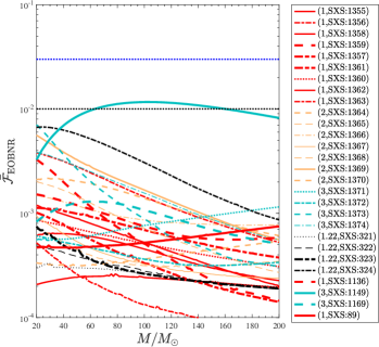
Figure 12: EOB/NR unfaithfulness for the $\ell=m=2$ mode computed over the eccentric SXS simulations publicly available using the ${\tt TEOB-Dali_{4PN-NRTuned}}$ model, analogous of Fig. 8 above. The unfaithfulness is much smaller except for a single outlier $\sim 1\%$. This configuration has $\tilde{a}_{0}=0.675$ and $\bar{{\cal F}}_{\rm EOBNR}^{\rm max}$, is consistent with the quasi-circular value, $\sim 0.01$, at $(3,0.675)$, as illustrated by the right panel of Fig. 11.

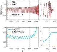
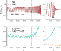
Figure 13: Eccentric case: understanding the unfaithfulness of Figs. 8 and 12 in terms of time domain phasing for SXS:BBH:1149, i.e. $(3,+0.70,+0.60)$. The left panel corresponds to Dali_4PN-analytic and the right panel to Dali_4PN-NRtuned. The worsening of the $\bar{{\cal F}}_{\rm EOBNR}^{\rm max}$ from $4\times 10^{-3}$ (in Fig. 8) to $\sim 10^{-2}$ in Fig. 12 is due to the (approximate) doubling of the phase difference at merger related to the improvable spin sector of Dali_4PN-NRtuned. See Sec. IV.1 for discussion.

The analysis we have carried out so far has highlighted the importance of the analytical choice made for the radiation reaction. In particular, it has shown that its effect cannot be completely absorbed/corrected by NR tuning $a_{6}^{c}$. We have two models with different performances versus NR waveforms. From the above discussion, it seems clear that the $3^{+2}$PN $\rho_{22}$ is too large and entails an incorrect phase acceleration, with a positive phase difference accumulated with respect to the NR waveform up to merger. On the other hand, the $P^{2}_{2}(\rho_{22}^{\rm 4PN})$ function, which is smaller, yields an accumulated phase difference up to merger is negative and nonnegligible. On the basis of this analysis we thus expect that a function that is slightly larger than $P^{2}_{2}(\rho_{22}^{\rm 4PN})$ might succeed in improving the EOB/NR phasing agreement up to the $0.01$ rad level during the latest orbits before the beginning of the plunge. As a first attempt, we took $\rho_{22}$ at $4^{+1}$PN with an effective 5PN parameter linear in $\nu$ that can be tuned. This is then resummed using either a $(2,3)$ or a $(3,2)$ Padé approximant. Unfortunately we find that in both cases the Padé approximant develops a spurious pole, which prevents us from following this route. As an alternative, we can, instead, still work at 4PN accuracy, but replace the exact 4PN $\nu$-dependence with an effective term of the form $\nu c_{4}^{\nu}x^{4}$ where $c_{4}^{\nu}$ is a parameter to be determined via EOB/NR comparison. Schematically, the 4PN term in $\rho_{22}$ thus reads $(c_{0}+\nu c_{4}^{\nu})x^{4}$, where now $c_{4}^{\nu}$ is a parameter intended to replace the analytical $\nu$ dependence of the function in Eq. (II.1). For consistency with our previous choice, we then take the $(2,2)$ Padé approximant, that now depends on $c_{4}^{\nu}$. It turns out that it is easy to tune $c_{4}$ to reduce the dephasing in the last part of the inspiral; similarly, one can additionally tune $a_{6}^{c}$ so to adjust the phase difference through late plunge, merger and ringdown, so to to have it negative and monotonically decreasing. By iteratively tuning both $c_{4}^{\nu}$ and $a_{6}^{c}$ one eventually finds that the best values approximately lie on two straight lines and can be accurately fitted as follows

$$a_{6}^{c} =-24.453-270.25\nu\ ,$$ (40)

$$c_{4}^{\nu} =5.3896-75.26\nu\ .$$ (41)

It is interesting to note that the fractional difference between the NR-tuned $c_{4}^{\nu}$ and the analytic one is at most $\sim 0.6\%$ around the LSO crossing. In the flux, this means $\sim 1.2\%$ fractional difference between the fluxes. Focusing first on the EOB/NR comparisons for nonspinning configurations, Fig. 10 gives us a flavor of the EOB/NR performance that can be achieved this way. In the top panel we show the time-domain phasing for two illustrative mass ratios, $q=1$ and $q=6$, while the bottom panels display $\bar{{\cal F}}_{\rm EOBNR}$ for 19 different values of $q$. The plot shows that an accumulated phase difference $\simeq 0.1$ rad translates in $\bar{{\cal F}}_{\rm EOBNR}\sim 10^{-4}$, the level of accuracy that we may expect to be needed for 3G detectors.

When considering spinning system, we have to determine a new expression of $c_{3}$ by EOB/NR phasing comparison. In doing so, one quickly realizes that the current implementation of the spin-dependent waveform terms yields an emission of gravitational radiation (and thus backreaction of the system) that exceeds the NR prediction: the transition from inspiral to plunge occurs too fast. This points us towards the identification of systematic inaccuracies also in this building block of the model, that thus should be modified accordingly. As a minimal attempt in this direction, for the $m={\rm even}$ modes up to $\ell=4$ we implement the orbital-factorized (and resummed) amplitudes introduced in Refs. [28, 29]. Analytical expressions constructed following this approach were found to agree well with the corresponding numerical data in the test-mass limit, although their potentialities were not explored in full in the comparable mass case. The $\rho_{\ell m}$’s residual amplitudes are written in orbital-factorized form

$$\rho_{\ell m}=\rho_{\ell m}^{\rm orb}\hat{\rho}_{\ell m}^{S}\ ,$$ (42)

and then both functions are resummed. The $\rho^{\rm orb}_{\ell m}$’s are the same considered in the previous section, i.e. are resummed using Padé approximants. The $\hat{\rho}_{{\ell m}}^{S}$ are instead replaced by their inverse-Taylor resummed expressions, $\bar{\rho}_{\ell m}^{S}$, that are defined as:

$$\bar{\rho}_{\ell m}^{S}=\left[T_{n}\left(\rho_{\ell m}^{-1}\right)\right]^{-1}\ ,$$ (43)

where $T_{n}$ indicates the Taylor expansion of order $n$. The $\bar{\rho}_{\ell m}^{S}$ are then functions that formally read:

$$\bar{\rho}_{\ell m}^{S} =\bigg{(}1+c^{\ell m}_{3/2}x^{3/2}+c^{\ell m}_{2}x^{2}$$

$$+c^{\ell m}_{5/2}x^{5/2}+c^{\ell m}_{3}x^{3}+c^{\ell m}_{7/2}x^{7/2}\dots\bigg{)}^{-1}\ ,$$ (44)

where $x$ is some (squared) velocity PN variables. Here integer powers correspond to terms even in the spins, while semi-integer powers to terms that are odd in the spin. In particular, up to $\ell=4$, the $m=\text{even}$ functions that we consider are explicitly given by:

$$\bar{\rho}_{22}^{S}=\Bigg{\{}1+\left(\dfrac{\tilde{a}_{0}}{2}+\dfrac{1}{6}X_{12}\tilde{a}_{12}\right)x^{3/2}-\dfrac{\tilde{a}_{0}^{2}}{2}x^{2}$$

$$+\left[\tilde{a}_{0}\left(\dfrac{337}{252}-\dfrac{73}{252}\nu\right)+X_{12}\tilde{a}_{12}\left(\dfrac{27}{28}+\dfrac{11}{36}\nu\right)\right]x^{5/2}$$

$$+\left[\tilde{a}_{0}^{2}\left(\frac{11}{42}+\dfrac{31}{252}\nu\right)+\tilde{a}_{1}\tilde{a}_{2}\left(\dfrac{19}{63}-\dfrac{10}{9}\nu\right)-\dfrac{179}{252}X_{12}\tilde{a}_{1}2\tilde{a}_{0}\right]x^{3}$$

$$+\left[\dfrac{2083}{2646}\tilde{a}_{0}-\dfrac{13}{12}a_{0}^{3}+X_{12}\tilde{a}_{12}\left(\dfrac{\tilde{a}_{0}^{2}}{12}+\dfrac{13367}{7938}\right)\right]x^{7/2}\Bigg{\}}^{-1},$$ (45)

$$\bar{\rho}_{32}^{S}=\left[1+\left(-\dfrac{\tilde{a}_{0}}{3-9\nu}+\dfrac{X_{12}\tilde{a}_{12}}{3-9\nu}\right)x^{1/2}\right]^{-1}\ ,$$ (46)

$$\bar{\rho}_{44}^{S}=\left[1+\left(\dfrac{19}{30}\tilde{a}_{0}+\dfrac{1-21\nu}{30-90\nu}X_{12}\tilde{a}_{12}\right)x^{3/2}\right]^{-1}\ ,$$ (47)

$$\bar{\rho}_{42}^{S}=\left[1+\left(\dfrac{\tilde{a}_{0}}{30}+\dfrac{19-39\nu}{30-90\nu}X_{12}\tilde{a}_{12}\right)x^{3/2}\right]^{-1}\ .$$ (48)

With this analytic choice, we proceed determining a new expression for $c_{3}$, with the same functional form discussed above. The corresponding fitting coefficients are listed in the second row of Table 3. The model, now dubbed Dali_4PN-NRtuned, is then validated computing the unfaithfulness (using Advanced Ligo sensitivity) with all SXS quasi-circular NR simulations. The result is reported in Fig. 11. The left panel of the figure shows $\bar{{\cal F}}_{\rm EOBNR}$ versus the total mass $M$, while the right panel gives $\bar{{\cal F}}^{\rm max}_{\rm EOBNR}$ versus $(\tilde{a}_{0},q)$. This analysis indicates that the tuning of the nonspinning flux eventually yields an improved EOB/NR agreement for negative and mild spins, with a global shift of all values towards the $10^{-4}$ goal. The performance for eccentric configurations is reported in Fig. 12. Not surprisingly, the NR-tuning of the nonspinning radiation reaction allows for a general reduction of the EOB/NR unfaithfulness even for eccentric bound systems. We similarly recompute the scattering angle for all configurations previously considered. The corresponding values are listed in Tables 5-6. Also in this case one sees that the NR-tuning of the (nonspinning) flux eventually yields an improve agreement between the NR and EOB scattering angles.

To better understand the impact of these changes on the EOB dynamics and put these numbers into perspective, it is instructive to observe how the changes in the model reflect on the potential energy. The left panel of Fig. 14 shows $E_{\rm circ}/M=\sqrt{1+2\nu(\hat{E}_{\rm eff}^{\rm circ}-1)}$ where $\hat{E}^{\rm circ}_{\rm eff}=A(1+p_{\varphi}^{2}u^{2})$ for configuration $\#1$ in Table 5 for various choices of the potential $A$. The black line corresponds to $\chi^{\rm EOB}_{\rm 4PN-Analytic}=346.83$, while the red curve to $\chi_{\rm 4PN-NRTuned}^{\rm EOB}=326.79$. The smaller value of the scattering angle is due to the fact that the peak of the potential energy, corresponding to the unstable orbit, is higher. By keeping the NR-informed 4PN-like radiation reaction, we find that fixing $a_{6}^{c}=-85$, instead of the value $a_{6}^{c}\simeq-92$ coming from Eq. (40), result in an increase of the peak of the potential energy such to yield for the scattering angle $\chi_{\rm EOB}=308.76$, i.e. with approximately $1\%$ fractional difference with the NR prediction $\chi_{\rm NR}=305.8$. This shows that it is actually possible to match the NR values consistently with their nominal error bars by just a fine tuning of the $A$ function (improved EOB/NR agreement is evidently found also for the other configurations).

An analogous explanation holds in the spinning case, as highlighted in Fig. 15. The figure refers to the second configuration of Table 6, $(1,-0.25,-0.25)$, with the NR-informed 4PN-effective radiation-reaction term. In this case, the EOB model predicts a plunge, while NR gives $\chi_{\rm NR}=367.55$ deg. Since the EOB and NR values in the nonspinning case are rather consistent, with a fractional difference $\sim 2\%$, we argue that the spin-sector, though NR-informed by quasi-circular simulations, might need to be further modified to properly match the NR scattering angle. In principle the effects are expected to be shared between both the conservative and nonconservative part of the spin-sector of the model. As a first exploratory step, we only decide to modify the Hamiltonian, looking for a value of $c_{3}$ such to yield an acceptable EOB/NR consistency. This is obtained by fixing $c_{3}=110$, that determines a rise in the peak of the potential such to yield $\chi_{\rm EOB}\simeq 363$. This corresponds to a large modification to the normalized gyro-gravitomagnetic functions $(\hat{G}_{S},\hat{G}_{S_{*}})$ shown in the right panel of Fig. 15. Clearly, this value of $c_{3}$ will not yield an accurate phasing in the quasi-circular case. This simple analysis thus highlights the complication of finding full consistency between the quasi-circular case and configurations that are close to direct plunge. By contrast, the flexibility (and robustness) of the model is such that each case can be matched accurately with the tuning of one single parameter. Note that these effects were already pointed out in Ref. [11], using however configurations with higher values of the (negative) spins. Finally, is worth stressing that the current analysis should be seen as essentially illustrative and qualitative. A reduction of the EOB/NR disagreement between scattering angles close to the threshold of capture might be also obtained by modifying other sectors of the model, like the radiation reaction or the noncircular part of the conservative dynamics, e.g. the $D$ function (see e.g. an exploratory analysis along these lines in Ref. [9]). Our findings are just supposed to highlight the delicate interplay of various effects in the subtle regime around the threshold of immediate merger and will deserve more dedicated studies in the future.

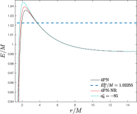
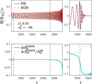
Figure 14: Configuration $\#1$ in Table 5, comparing different potential energies that yield different values of the scattering angle.

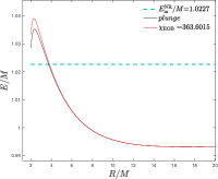
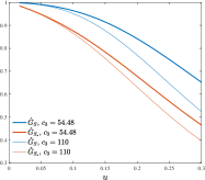
Figure 15: Configuration $\#1$ in Table 6 $(1,-0.25,-0.25)$. Left panel: the potential energy. Right panel, the gyro-gravitomagnetic ratios. The value $c_{3}=110$ corresponds to the red curve in the left panel that yields a value of the angle compatible with the NR one. To do so, the magnitude of the spin-orbit coupling has to be reduced with respect to standard case (thick line versus thin lines in the right panel).

IV.1 Discussion: understanding the results

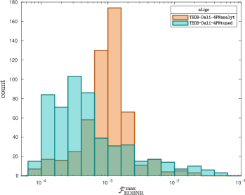
Figure 16: Quasi-circular limit: comparing $\bar{{\cal F}}_{\rm EOBNR}^{\rm max}$ for Dali_4PN-analytic and Dali_4PN-NRtuned. Despite the tail towards values of $\bar{{\cal F}}_{\rm EOBNR}^{\rm max}\sim 0.1$ (corresponding to large, positive, spins), thanks to the NR-tuning of the (nonspinning) flux, Dali_4PN-NRtuned performs globally better all over the SXS catalog of spin-aligned waveforms, with median $\sim 3.92\times 10^{-4}$. The corresponding value for Dali_4PN-analyticis instead $1.06\times 10^{-3}$, although $\bar{{\cal F}}_{\rm EOBNR}^{\rm max}$ is at most $\sim 0.01$. The performance of Dali_4PN-NRtuned suggests that a careful NR-tuning of the dissipative part of the dynamics might be eventually needed to construct a highly faithful (say $\simeq 10^{-4}$) model all over the BBH parameter space.

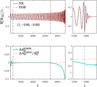
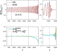
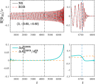
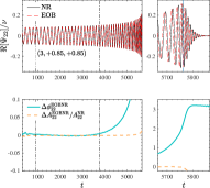
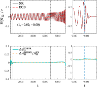
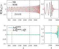
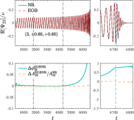
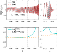
Figure 17: Quasi-circular case: understanding the unfaithfulness of Figs. 5 and 11 with selected time-domain phasing analysis. Top panels: model Dali_4PN-analytic. Bottom panels: model Dali_4PN-NRtuned (that also differs for the spin part of radiation reaction). The bottom-left panels show the excellent EOB/NR phasing agreement brought by the NR-tuning of the flux. By contrast, progressively large dephasings as the spins are increased are found because of inaccuracies in the spin-dependent part of the flux. This well explains the behavior of $\bar{{\cal F}}_{\rm EOBNR}^{\rm max}$ shown in the right panel of Fig. 11. Note in particular that in the bottom-right panel the phase difference is nonmonotonic in time around merger, which eventually yields large values of $\bar{{\cal F}}_{\rm EOBNR}$.

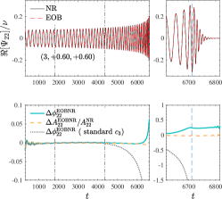
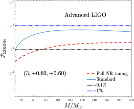
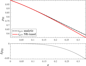
Figure 18: Proof of principle: effect of tuning, at the same time, the spin-dependent part of the waveform (and radiation reaction), with an effective 3.5PN coefficient, and the N³LO effective spin-orbit parameter $c_{3}$. The phase difference during the early inspiral is now flat (cf. the corresponding panel in the bottom row of Fig. 17) and approximately zero, increasing then monotonically up to only $\sim 0.2$ rad around merger (left panel). Consistently, the EOB/NR unfaithfulness (middle panel) is at most $\sim 1.9\times 10^{-3}$ for large masses. The right panel shows the reduction of the NR-tuned $\rho_{22}$ with respect to the analytical one. This entails a fractional reduction of $\sim 10\%$ in the radiation reaction force around $x\sim 0.2$, that eventually yields the dotted-line phase difference in the leftmost panel of the figure. The further tuning of $c_{3}$ yields the $\sim 0.2$ rad at merger displayed and the rather low $\bar{{\cal F}}_{\rm EOBNR}\sim 10^{-3}$ all over the mass range.

So far we have explored two, different, NR-informed routes to obtain an eccentric waveform model that is consistent with the quasi-circular, spin-aligned, SXS waveform data as well as with the NR surrogates NRHybSur3dq8 and NRHybSur2dq15. In one case, we use 4PN-resummed analytical radiation reaction and we find a satisfactory model with $\bar{{\cal F}}_{\rm EOBNR}^{\rm max}\simeq 1\%$ all over the parameter space of spin-aligned quasi-circular configurations. In the other case, we additionally NR-tune the spin-independent part of the radiation reaction force and change the analytic description of the $m=even$ waveform (and radiation) modes up to $\ell=4$: this gives rather low EOB/NR unfaithfulness values for negative and mildly positive values of the effective spin ($10^{-4}\lesssim{\bar{{\cal F}}}_{\rm EOBNR}^{\rm max}\lesssim 10^{-3}$), though they can be as large as a few parts in $10^{-2}$ for large, positive spins. The performance of both models is summarized in Fig. 16, that shows together the two distributions of $\bar{{\cal F}}_{\rm EOBNR}^{\rm max}$. Despite the tail towards values of $\bar{{\cal F}}_{\rm EOBNR}^{\rm max}\sim 0.1$ (corresponding to large, positive, spins), the model with the NR-informed, effective, 4PN radiation reaction (and waveform) performs globally better all over the SXS catalog, with median $\sim 3.92\times 10^{-4}$, approximately three times smaller than the $1.06\times 10^{-3}$ corresponding to the 4PN analytical model. This suggests that a careful NR-tuning (or at least analytical improvement) of the dissipative part of the (spin-dependent) dynamics might be eventually needed to construct a highly faithful (say $\simeq 10^{-4}$) model all over the BBH parameter space. Although this task is beyond the scope of the present work, it is pedagogically useful to connect some selected values of $\bar{{\cal F}}^{\rm max}_{\rm EOBNR}$ to the time-domain phasing, so to get a sense of their actual meaning. This is done in Fig. 17 for four selected configurations. The top row of the figure is obtained with the Dali_4PN-analytic model, while the bottom panel with the Dali_4PN-NRtuned model. The leftmost panels, $(1,-0.60,-0.60)$ and $(3,0,0)$, connect the values ${\cal F}^{\rm max}_{\rm EOBNR}\simeq 10^{-4}$ with phase differences around merger $\lesssim 0.05$ rad. Similarly, the increase of the values of $\bar{{\cal F}}^{\rm max}_{\rm EOBNR}$ for larger spins is mirroring either a larger value of $\Delta\phi^{\rm EOBNR}_{22}$ at merger, or the fact that the phase difference is not monotonic through late plunge, merger and ringdown. As throughly discussed in Ref. [13] this is one of the features of the phase difference that is mirrored into large values of $\bar{{\cal F}}_{\rm EOBNR}^{\rm max}$. The fact that the phasing inaccuracies increase with the value of the effective spin $\tilde{a}_{0}$ is explained as follows. The figure shows that, for both models, and in the presence of positive spins, the EOB dynamics predicts a transition from inspiral to plunge and merger that is less adiabatic (i.e., faster) than the NR one, with a (positive) phase difference that accumulates progressively during the late inspiral. This phase difference cannot be reduced only by the tuning of the dynamic parameter $c_{3}$, as it happens at spatial separations (or frequencies) where its tuning is practically ineffective. The reason for this is that $c_{3}$ parametrizes spin-orbit corrections that are proportional to $r^{-3}$, and thus that become important only when $r$ is small enough. In any case, the fact that the phasing predicted by Dali_4PN-NRtuned is highly NR-faithful for $(3,0,0)$, with a dephasing of approximately $-0.02$ rad at merger, while it is not for larger spins indicates that the spin sector of the model should be improved in some way. Improving the spin sector means controlling the subtle interplay between conservative and nonconservative effects, similarly to what we discussed already in the nonspinning case. In particular, the fact that the phase difference is positive and grows during the late inspiral already suggests that the radiation reaction force is inaccurate as the two objects get close and should be modified in some way. We thus explore, as a proof of principle, whether the EOB/NR agreement can be improved by NR-tuning, at the same time, the spin-dependent part of the radiation reaction and consistently the spin-orbit Hamiltonian via $c_{3}$. Focusing on $\bar{\rho}_{22}^{S}$, we recall that it is given in inverse resummed form at NNLO (i.e., 3.5PN accuracy). As a first attempt, we explored the effect of adding higher-order terms (i.e., beyond 3.5PN) to Eq. (IV). Such terms, notably $(c_{4}^{22}x^{4},c_{9/2}x^{9/2},c_{5}x^{5})$, were obtained by extrapolating to the comparable mass case the corresponding terms in the test-particle limit, following the procedure introduced in Sec. VB of Ref. [29]. Not surprisingly, we found no effect on the late-inspiral behavior. We decided then to tune an effective 3.5PN term, i.e. replacing the analytical $c_{7/2}^{22}$ coefficient with an effective one. Since our aim is only to understand the origin of the physical effect, we consider the single configuration $(3,+0.60,+0.60)$. Analogously to the nonspinning case discussed above, we realized that it is possible to tune, iteratively, both $(c_{7/2}^{22},c_{3})$, so to reduce the EOB/NR phase difference through the late inspiral, merger and ringdown and have it growing monotonically with time. Figure 18 reports our final result: it is obtained with $c^{22}_{7/2}=3.1$ and $c_{3}=33.8$. Analytically, for this configuration (from Eq. (IV)) one has $c^{22}_{7/2}=0.49$ and the previously NR-tuned value of $c_{3}$ was $c_{3}=21.11$ The meaning of these numbers is as follows. One needs to reduce the action of the analytical radiation reaction (and thus the amplitude $\bar{\rho}_{22}^{\rm S}$) so to slow the rate of inspiral down. The value $c^{22}_{7/2}=3.1$ corresponds to the red line in the rightmost panel of Fig. 18, that lies below the analytical curve. One has a fractional difference of $\sim 2\%$ at $x\sim 0.20$, that corresponds to a (fractional) reduction of the flux of $\sim 10\%$ at the same value of $x$. The effect of this reduction on the EOB/NR phase difference is illustrated by the dotted, gray, line in the leftmost panel of Fig. 18, that however still retains $c_{3}=21.11$, as obtained from the second row of Table 3. At this stage, it is additionally possible to modify $c_{3}$, and thus reduce the magnitude of the spin-orbit interaction (i.e., shortening the EOB waveform), until one obtains the $\Delta\phi_{22}^{\rm EOBNR}$ curve depicted in light blue in the leftmost panel of the figure. This corresponding to $c_{3}=33.8$. As mentioned above, this result was obtained tuning iteratively the two parameters whose action is, partly, degenerate. Although it is certainly possible to increase both parameters to further reduce the phase difference at merger, we here content ourselves to show that this is feasible and that it is necessary to NR-tune the radiation reaction force so to obtain an inspiral waveform that is more NR-faithful. Although in this case we reached this goal by tuning one additional parameter, it might be possible that other analytical representation of the resummed waveform (and radiation reaction) exist such to eventually yield a similar result. The important take away message is that an improved analytical representation of the (spin-dependent) part of the flux might be important in order to get to the $10^{-4}$ unfaithfulness level also for large-positive spins.

V Conclusions

In this work we present an updated model for spin-aligned, coalescing black hole binaries for generic (i.e., noncircularized) planar orbits, from eccentric inspirals to scattering configurations. This model builds upon, improves and replaces previous work in the TEOBResumS lineage [2, 9, 7, 10, 17, 4, 13], notably Refs. [10, 13]. The most important feature of the new eccentric model is that its quasi-circular limit shows an excellent consistency with the latest avatar of the quasi-circular model TEOBResumS-GIOTTO [13]. The new physical understanding of this paper is a fresh look at the importance of the radiation reaction force in correctly modeling the late-inspiral dynamics and waveform. In particular, we explored the influence of various version of the azimuthal component, ${\cal F}_{\varphi}$, that drives the backreaction on the orbital motion due to the loss of angular momentum through gravitational waves. We thus analyze the class of analytic waveform systematics related to the dissipative part of the dynamics, complementing similar studies reported in Refs. [7, 13] that were focused only on systematics related to changes to the conservative part of the dynamics. In doing this exploration, we ended up with two different, though consistent, prescriptions for building an improved waveform model for eccentric binaries. These two main results can be summarized as follows.

• We took advantage of the recently computed 4PN waveform terms in the $\ell=m=2$ mode [21, 22, 23] and updated the model with this new analytical information. We argued that the use of a resummed 4PN residual amplitude is important and carefully compared (in the nonspinning case) the performance of the $\rho_{22}^{\rm 4PN}$ with the $\rho_{22}$ at $3^{+2}$PN accuracy used in all implementations of TEOBResumS since 2009 [27]. We clarified that in one case the actual flux seems to be overestimated (and thus the transition from inspiral to plunge occurs faster than the NR prediction) while in the other case it is slightly underestimated (and thus the transition is slower), although in this second case the performance of the model is generally better. Therefore, we conclude that the 4PN-resummed $\rho_{22}$ function looks like the current best analytical choice to build EOB radiation reaction and waveform. The model is then informed by quasi-circular NR-data so as to determine the usual coefficients $(a_{6}^{c},c_{3})$, respectively modeling effective 5PN correction in the orbital interaction potential and effective 4.5PN (or N³LO) spin-orbit effects [32]. The model performance is then evaluated all over the parameter space currently covered by public NR simulations or data, in particular: (i) in the quasi-circular limit, it is compared with the full SXS catalog [51] of public NR simulations (up to $q=15$) as well as with the quasi-circular NR surrogates NRHybSur3dq8 and NRHybSur2dq15; (ii) for eccentric inspiral, it is compared with the 28 public SXS simulations; (iii) scattering angles. Figure 6 shows the excellent consistency between TEOBREsumS-GIOTTO [13] and the 4PN-based TEOBResumS-Dali model for quasi-circular configurations. For the considered eccentric configurations, $\bar{{\cal F}}^{\rm max}_{\rm EOBNR}$ is always well below $1\%$ (except a single outlier, that also corresponds to a rather noisy dataset). Furthermore, the scattering-angle comparisons (see Table 5) are satisfactory and consistent with previous literature.

• From the understanding that $\rho_{22}^{\rm 4PN}$ underestimates the effect of the actual radiation reaction, while $\rho_{22}^{3^{+2}}$ overestimates it, we decided to attempt charting an unexplored territory by NR-informing, at the same time both the conservative and nonconservative part of the EOB dynamics. This is done NR-tuning both $a_{6}^{c}$ and an effective 4PN term entering the Padé resummed $\rho_{22}^{\rm 4PN}$ that replaces the analytical 4PN information of Ref. [21]. In the nonspinning case, one finds that just a small modification to the analytically known $P^{2}_{2}(\rho_{22}^{\rm 4PN})$ (together with a new $a_{6}^{c}$) is by itself sufficient to bring the EOB/NR phase difference at merger below $\sim 0.1$ rad, a value that is consistent with the expected NR uncertainty. This results in $\bar{{\cal F}}_{\rm EOBNR}^{\rm max}\sim 10^{-4}$ for all available nonspinning datasets up to mass ratio $q=15$. In the presence of spins, we, again, clearly highlighted the importance of the spin-dependent part of the radiation reaction and evaluated the influence of different analytical prescriptions for the resummed EOB waveform that were discussed in the literature. For example, we concluded that the additive expression $\rho_{22}^{\rm orb}+\rho_{22}^{\rm S}$ implemented in any version of TEOBResumS is overestimating the flux for positive spins and that a better (though certainly improvable) representation of the residual amplitude corrections is obtained by the factorized and inverse-resummed prescription discussed in Refs. [28, 29]. With this choice, and a new expression of the NR-informed $c_{3}$, we may eventually end up having a model, dubbed TEOBResumS-Dali-4PNTuned, that is globally more NR faithful than the current TEOBResumS-Dali. A new look at the analytical representation of the EOB-resummed radiation reaction is postponed to future work.

In conclusion, we have now at hand two waveform models for non-circularized binaries that differ because of (i) the analytic content and (ii) the amount of NR-information included. Although in the quasi-circular limit none of these two model is as NR-faithful as TEOBResumS-GIOTTO, they will hopefully allow us to give a very precise quantitative meaning to the actual impact of waveform systematics on current and future GW detectors [44, 52].

P.  R. and S. B. thank the hospitality and the stimulating environment of the IHES, where part of this work was carried out. We thank M. Panzeri for cross-checking some results presented in Appendix A and G. Carullo for comments and a careful reading of the manuscript. The present research was also partly supported by the “2021 Balzan Prize for Gravitation: Physical and Astrophysical Aspects”, awarded to Thibault Damour.

Appendix A Alternative Padé resummation of $\rho_{22}$ and implications.

In Sec. II.1 the $\rho_{22}^{\rm 4PN}$ function was resummed by taking a global Padé approximant obtained by replacing the $\log(x)$ terms with some formal constants and then reinserting them back. Historically this has been a standard approach within the EOB model (see e.g. Ref. [27] and references therein), that, however, was never carefully tested with alternatives. It should also be noted that in the test-mass limit this approach was extensively used in Refs. [28, 29] and found sufficiently satisfactory at the time. In this Appendix we point out that this method introduces some analytic systematics that were overlooked so far and that might be important at the level of accuracy we are currently pushing our models. Despite this, the results discussed in the main text are expected to stand even against these systematics. To start with, let us review in detail our resummation procedure so to highlight its drawbacks. The 4PN-accurate function of Eq. (II.1) schematically reads

$$\rho=1+c_{1}x+c_{2}x^{2}+x^{3}[c_{3}+c_{3}^{\log}\log(x)]+x^{4}[c_{4}+c_{4}^{\log}\log(x)]\ ,$$ (49)

For pedagogical purpose, let us first assume all the coefficients equal to one. Then, one poses $\log(x)=c$ and takes the $(2,2)$ Padé approximant. This reads

$$\rho^{\prime}\equiv P_{2}^{2}(\rho)=\dfrac{1+x-cx^{2}}{1-(1+c)x^{2}}\ .$$ (50)

There are two sorts of inconsistencies. First, by expanding this expression in powers of $c$, we find

$$\rho^{\prime}=\frac{1}{1-x}+\frac{x^{3}}{(1+x)(1-x)^{2}}c+O(c^{2})\ ,$$ (51)

and we should compare it with the original function $\rho$, Eq. (49), after replacing $c$ with $\log(x)$. In particular, we notice that even though

$$\frac{x^{3}}{(1+x)(1-x)^{2}}-(x^{3}+x^{4})=O(x^{5})\ ,$$ (52)

which is consistent with the error of Padé approximation, the rational function $\frac{x^{3}}{(1+x)(1-x)^{2}}$ has a degree $3$ denominator which is an unreasonable approximation of $x^{3}(1+x)$.

Second, by expanding $\rho^{\prime}$ in Eq. (50) at higher order, e.g. 5PN, we have

$$\rho^{\prime} \sim 1+x+x^{2}+(1+c)x^{3}+(1+c)x^{4}$$

$$+(1+c)^{2}x^{5}+O(x^{6})\ .$$ (53)

When the constant $c$ is replaced by the $\log(x)$, one immediately sees that a 5PN term of the form $\log^{2}(x)x^{5}$ appears. In the general case, where the coefficients are not equal to one, the 5PN term guessed by the Padé approximant has the structure

$$c_{\rm 5PN}^{\rm guess}=\dfrac{n_{0}+n_{1}c+n_{2}c^{2}}{d1+d_{2}c}\ ,$$ (54)

Table 7: Fractional differences $\delta\rho_{22}=(\rho_{22}^{X}-\rho_{22}^{\rm Exact})/\rho_{22}^{\rm Exact}$ at $x_{\rm LSO}=1/6$ obtained with different analytical approximations. The function where the $\log(x)$ are treated separately is generally closer to the exact data at each PN order.

	Padé $\log(x)$ separated	Padé $\log(x)=c$	Taylor
4PN	$-0.000950$	$-0.004563$	$0.001804$
5PN	$-0.001234$	$-0.001358$	$-0.001621$
6PN	$-0.000317$	$-0.000654$	$-0.000425$
7PN	$-0.000187$	$-0.000393$	$+0.000001$
8PN	$-0.000168$	$-0.000143$	$-0.000106$

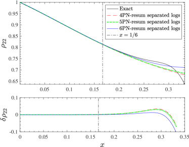
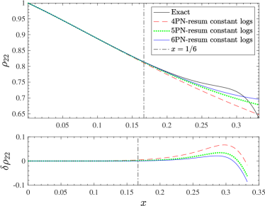
Figure 19: Test-mass limit ($\nu=0$). Resummed $\rho_{22}$ at 4PN, 5PN and 6PN using Padé approximants $(2,2)$, $(3,2)$ and $(4,2)$, accordingly to the PN order. Left panel: factorize the logarithmic terms and separately resum the polynomial coefficients. Right panel: set $c=\log(x)$, resum the polynomial with parameter $c$, and finally substitute back $c=\log(x)$. The bottom panels show the relative differences with the exact curve obtained numerically, $\delta\rho_{22}\equiv(\rho_{22}^{X}-\rho_{22}^{\rm Exact})/\rho_{22}^{\rm Exact}$.

where, again, the $c=\log(x)$. So, in the general case, the PN expansion of the Padé where the logarithms are considered as constant introduces an even more intricate logarithmic structure. Unfortunately, this is qualitatively inconsistent with the PN expansion of $\rho_{22}$, where the $\log^{2}(x)$ terms are know to only appear at 6PN order, as first shown in Ref. [53], Eq. (7) therein. The same inconsistency pointed out here at 4PN is present also in the 6PN-based resummed amplitude of Refs. [29], where a $(4,2)$ Padé approximant (with constant logs) was used for most multipoles. This affects, quantitatively, the (test-mass) radiation-reaction driven dynamics of Refs. [54, 55, 14] as well as the comparable-mass dynamics of several works that were incorporating the approach of Ref. [29] where different versions of TEOBResumS were developed, e.g. Refs. [30, 13]. Nonetheless, it should be noted that, since the EOB dynamics is additionally informed by NR simulations, this inconsistency is not expected to have a dramatic influence on well established results. In this respect, in the main text we showed that a NR-informed effective 4PN term, within the same Padé resummed structure, may eventually yield an improved waveform model, with unfaithfulness $\simeq 10^{-4}$. This, together with the inconsistency in our resummation strategy, calls for an alternative approach to resumming $\rho_{22}^{\rm 4PN}$ such that the trascendental structure of the function is preserved. A very simple procedure consists in resumming separately the polynomial part and the terms that are proportional to the $\log(x)$. In this way, the trascendental order of the function is guaranteed not to be changed by the resummation procedure and, a priori, we may expect results more consistent with the exact function. Schematically, $\rho_{22}^{\rm 4PN}$ can be recasted as

$$\rho_{22}^{\rm 4PN}(x)=p_{0}^{(4)}(x)+p_{\log}^{(4)}(x)\log(x)\ ,$$ (55)

where $p_{0}^{(4)},p_{\log}^{(4)}$ are polynomials of the form

$$p_{0}^{(4)}(x) =1+c_{1}x+c_{2}x^{2}+c_{3}x^{3}+c_{4}x^{4}\ ,$$ (56)

$$p_{\log}^{(4)}(x) =c_{3}^{\log}x^{3}+c_{4}^{\log}x^{4}\ .$$ (57)

Then, we resum $p_{0}^{(4)}$ and $p_{\log}^{(4)}$ separately. For $p_{0}^{(4)}$ we use a $(2,2)$ Padé approximant. For $p_{0}^{(4)}$, we factorize the $x^{3}$ term in front and the rest is resummed taking at $(0,1)$ Padé approximant. When evaluated in the test-mass limit, the resulting analytical function is found to be closer to the exact one, obtained numerically (see e.g. [29] and references therein), than the our standard choice discussed in the main text. In particular the fractional difference at $x_{\rm LSO}=1/6$ is $\sim-0.000969$ versus the value $-0.00456$ obtained with the Padé approximant with constant logs. We will come back to the impact of this case on the comparable-mass case below. Before this, since most of the established test-mass results mentioned above are based on 6PN-accurate $\rho_{\ell m}$’s (see Table I in Ref. [29]), we also briefly investigate the effect of the new resummation at 6PN. A more comprehensive analysis of all multipoles will be reported elsewhere [56]. Schematically, $\rho_{22}^{\rm 6PN}$ can be recasted as

$$\rho_{22}^{\rm 6PN}(x)=p_{0}^{(6)}(x)+p_{\log}^{(6)}(x)\log(x)+p_{\log^{2}}^{(6)}(x)\log^{2}(x)\ ,$$ (58)

where $p_{0}^{(6)},p_{\log}^{(6)},p_{\log^{2}}^{(6)}$ are polynomials of the form

$$p_{0}^{(6)}(x) =1+c_{1}x+c_{2}x^{2}+c_{3}x^{3}+c_{4}x^{4}+c_{5}x^{5}+c_{6}x^{6}\ ,$$ (59)

$$p_{\log}^{(6)}(x) =c_{3}^{\log}x^{3}+c_{4}^{\log}x^{4}+c_{5}^{\log}x^{5}+c_{6}^{\log}x^{6}\ ,$$ (60)

$$p_{\log^{2}}^{(6)}(x) =c_{6}^{\log^{2}}x^{6}\ .$$ (61)

Then we observe that resumming only $p_{0}^{(6)}$ (and taking the Taylor expansion of $p_{\log}^{(6)}$ and $p_{\log^{2}}^{(6)}$) gives a better approximation than resumming both $p_{0}^{(6)}$ and $p_{\log}^{(6)}$. For $p_{0}^{(6)}$ we use a $(4,2)$ Padé approximant. As already noticed at 4PN, when evaluated in the test-mass limit, the resulting analytic function is found to be closer to the exact one, obtained numerically than our standard choice discussed. In particular the fractional difference at $x_{\rm LSO}=1/6$ is $\sim-0.000317$ versus the value $-0.000654$ obtained using a $(4,2)$ Padé approximant with constant logarithms. This suggests that at 6PN the logarithmic terms $p_{\log}^{(6)}$ and $p_{\log^{2}}^{(6)}$ are well approximated by the Taylor expansion, while the polynomial part $p_{0}^{(6)}$ needs to be resummed. The same reasoning applies at 7PN and 8PN, where we observe that resumming only the polynomial part gives a better approximation than resumming separately the polynomials and the logarithic terms . We collect the fractional differences at $x_{\rm LSO}=1/6$ in Table 7. Notably, comparing the fractional differences at $x_{\rm LSO}=1/6$, the resummation procedure described above gives a better approximation than the Taylor expansion (an exception, just by chance, is given by the 7PN, while at 8PN they are essentially equivalent). In addition, looking at the fractional differences, we see that resumming only the polynomial part is stable from 6PN to 8PN. The stability of this resummation at higher PN orders will be investigated elsewhere [56]. A priori we expect the scheme to remain robust up to 10PN, but things might become more subtle at higher orders, since fractional powers of $x$ appear. Whereas, going from 4PN to 6PN, we saw that different resummation methods of $\rho_{22}$ are effective as shown in Fig. 19; in particular, the logarithmic terms were resummed with a Padé approximant only at 4PN and 5PN, and they were not resummed at 6PN. Furthermore, at 6PN we also have $\log^{2}(x)$ terms which give a better approximation of the singular behavior of $\rho_{22}$. Hence, the different summation procedures at 4PN and 6PN can be justified as follows: Padé approximants of $p_{0}^{(k)}$ for $k=4,5,6$ capture well the singular behavior of $p_{0}(x)$ which seems “dominant” also at lower PN orders. Conversely, from 6PN (and at least up to 8PN) the singular behavior of $p_{\log}(x)+\log(x)p_{\log^{2}}(x)$ is better captured by the presence of $\log^{2}(x)$, thus the Taylor expansion of $p_{\log}$ gives a good approximation. Figure 19 summarizes our results at 4PN, 5PN and 6PN comparing the old resummation strategy (left panel) with the new one (right panel). It is remarkable the improvement found already at 4PN.

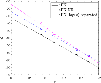
Figure 20: New values of the NR-informed $a_{6}^{c}$ obtained using the resumed $\rho_{22}^{\rm 4PN}$ based on the $\log$-separation of Eqs. (56)-(57). Note that the values of $a_{6}^{c}$ are close to the values corresponding to the NR-informed $c_{4}^{\nu}$ coefficient, but progressively differ as $\nu$ decreases. This has implications on the phasing and the global EOB/NR performance of the model, that turns out to get improved with respect to the versions discussed in the main text.

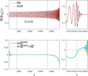
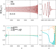
Figure 21: EOB/NR time-domain phasings for $q=1$ and $q=6$. The EOB performance is comparable to the case with the NR-informed flux discussed in the main text, see Fig. 10.

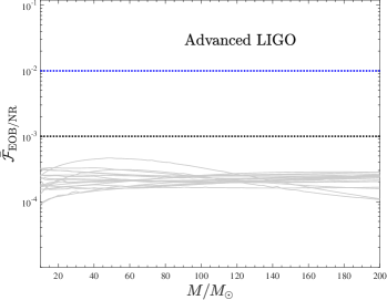
Figure 22: EOB/NR unfaithfulness for nonspinning configurations up to $q=15$. It is remarkable that the global EOB performance is substantially comparable to the left panel of Fig. 10, where the radiation reaction was also tuned to NR simulations.

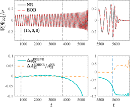
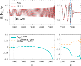
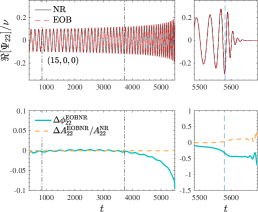
Figure 23: EOB/NR phasing for $q=15$ comparing three different representations of $\rho_{22}$ (at formal 4PN accuracy) with the corresponding values of $a_{6}^{c}$. Left panel: analytical 4PN with Padé $(2,2)$ resummation taking the $\log(x)$ as constant. Middle panel: same function but with the NR-tuned effective $c^{\nu}_{4}$ term of Eq. (41). Right panel: new resummation of $\rho_{22}^{\rm 4PN}$ separating the $\log(x)$’s from the rational part as described in Appendix A. The reduction of the EOB/NR dephasing at merger in this case is evident.

Now that we have a better understanding of the test-mass case, let us move to considering comparable mass binaries. We work then with $\rho_{22}^{\rm 4PN}$ resummed as described above (evidently, including the $\nu$-dependent terms) that thus yields a new waveform amplitude and radiation reaction. We then NR-inform a new function $a_{6}^{c}=-14.24-320.26\nu$, whose behavior is shown in Fig. 20. It is interesting to note that for $\nu\sim 0.25$ the values are compatible with those obtained with the NR-informed value of $c_{4}^{\nu}$. By contrast, the slope of the straight line is different than before. The model performance is then evaluated by computing either phasings in the time domain or the EOB/NR unfaithfulness with the SXS datasets available. We remind the reader that we consider mass ratios $1\leq q\leq 10$ spaced by 0.5 as well as the $q=15$ dataset of Ref. [47]. Figure 22 shows that, on the $\bar{{\cal F}}_{\rm EOBNR}$ quantity, the model performance gives, on average, $\bar{{\cal F}}_{\rm EOBNR}^{\rm max}\sim 10^{-4}$ and it substantially equivalent to the same analysis done with the NR-tuned $c_{4}^{\nu}$, see Fig. 10. This remarkable fact suggests the following two considerations. On the one hand it is an example that, by a (simple) improvement on the analytical side, one can obtain an excellent waveform model reducing the amount of NR-tuning . This is an important conceptual lesson that should be kept in mind for future studies (see below). On the other hand one has here an example of the extreme robustness of our EOB framework: even when an analytic systematic is present, it can be corrected by careful NR-tuning of some parameters and the actual performance without this systematic can be (substantially) obtained. It must be noted, however, that the model with the new $a_{6}^{c}$ and resummation of $\rho_{22}$ actually performs better than the totally NR-tuned one. This is apparent for the $q=15$ case. Figure 23 shows the EOB/NR time-domain phasing for the three models considered in the paper. From left to right: (i) Padé resummation of $\rho_{22}^{\rm 4PN}$ with the $\log(x)$ taken as constant when doing the Padé, NR-tuning of $a_{6}^{c}$ only; (ii) same Padé approximant but tuning both $(a_{6}^{c},c_{4}^{\nu})$; (iii) the model discussed in this Appendix. It is remarkable that the dephasing at merger in this case is $\sim 0.3$ rad, with more than a factor two gained with respect to the standard approach. We may argue that additional improvement should be brought once that a similar treatment of the $\log(x)$-dependent term is applied also to the subdominant modes, that are more relevant in this case than for $q=1$. Let us finally mention that the same problem with the Padé resummations performed under the assumption $\log(x)=c$ is present also in the EOB conservative dynamics, through the functions $A$ and $\bar{D}$ that are similarly resummed as discussed in Ref. [10]. As a preliminary investigation, we considered the 5PN accurate Taylor-expanded $A$ (with $a_{6}^{c}$ undetermined parameter) and resummed it using a $(3,3)$ Padé approximant for the polynomial part and a $(0,1)$ one for that proportional to the $\log(x)$’s, once that the term $u^{5}\log(u)$ is factored out. In the adiabatic limit, one finds that the new resummed function (and in particular the effective photon potential $u^{2}A$) is sufficiently flexible to match the one obtained with the current model once a suitable value of $a_{6}^{c}$ is chosen, that is found again to be linear in $\nu$. In conclusion, we state that the results discussed in the main text are expected to stand (and possibly improve) even with the correct treatment of the $\log$-dependent terms in the potentials. This analysis is currently in progress and will be detailed elsewhere [56]

Appendix B Eccentric initial conditions

Determining the initial conditions for eccentric bound systems in the EOB formalism is equivalent to finding the mapping between the desired initial eccentricity $e_{0}$, true anomaly $\zeta_{0}$ and some reference frequency $\Omega_{0}$ and the EOB dynamical parameters $(r_{0},p_{r*,0},p_{\varphi,0})$. In previous iterations of TEOBResumS, for simplicity and without loss of generality, the value of the anomaly $\zeta_{0}$ was fixed to either $0$ or $\pi$. This implied that – in order for all possible orbits to be covered during parameter estimation – the initial eccentricity $e_{0}$ and the initial frequency $\Omega_{0}$ had to be treated as free parameters [2, 7, 4]. Further, the user-specified initial frequency $\Omega_{0}$ was interpreted as the average frequency between periastron and apastron, $\Omega_{0,\rm avg}=(\Omega_{+}+\Omega_{-})/2.$ (see Appendix C of Ref. [7] for details). In this work, we implement an alternative approach to determine the initial conditions for eccentric orbits, which allows to fix the value of the true anomaly $\zeta_{0}$ to any desired value and allows for users to specify an initial orbit-averaged frequency $\bar{\Omega}_{0}$ as input parameters. This approach follows the one described in [20], and relies on the following steps:

• Given a set of initial conditions $(e_{0},\zeta_{0},\bar{\Omega}_{0})$, we compute the istantaneous frequencies at apastron and periastron $\Omega_{\pm}$ via the Newtonian expression:

  $$\Omega_{\pm}=\frac{\bar{\Omega}_{0}(1\pm e_{0})^{2}}{1-e_{0}^{2}}^{3/2}\,.$$ (62)

  From the istantaneous frequencies at apastron and periastron we then estimate $\Omega_{0,\rm avg}$.

• Recalling that

  $$r=\rho_{0}/(1+e_{0}\cos(\zeta_{0}))\,,$$ (63)

  we numerically find the initial semilatus rectum $\rho_{0}$ and radial momentum $p_{r*,0}$ by imposing that the average frequency is the desired one:

  $$\begin{split}2\Omega_{0,\rm avg}&=\frac{d\hat{H}}{dp_{\varphi}}(r(\rho_{0},e_{0},\zeta_{0}=0),j_{0}(\rho_{0},e_{0}),p_{r*0}=0)\\ &+\frac{d\hat{H}}{dp_{\varphi}}(r(\rho_{0},e_{0},\zeta_{0}=\pi),j_{0}(\rho_{0},e_{0}),p_{r*0}=0)\,.\end{split}$$ (64)

  and ensuring energy conservation at the point specified by $\zeta_{0}$:

  $$\begin{split}\hat{H}_{\rm eff}(r(\rho_{0},e_{0},\zeta_{0}=0),j_{0}(\rho_{0},e_{0}),p_{r*0}=0)=\\ \hat{H}_{\rm eff}(r(\rho_{0},e_{0},\zeta_{0}),j_{0}(\rho_{0},e_{0}),p_{r*0})\,.\end{split}$$ (65)

  In the equations above, $j_{0}$ is the value of angular momentum obtained by imposing energy conservation at apastron and periastron.

We note that these initial conditions are adiabatic, meaning that they do not incorporate effect of radiation reaction. While this approximation is expected to not lead to significant errors for large eccentricities, in the quasi-circular limit it is known that non-adiabatic initial data can lead to some spurious eccentricity in the waveforms [57, 58] Given that we find such spurious eccentricity to be of the order of $10^{-3}$, we expect this to be a minor effect with respect to other differences between the two TEOBResumS and TEOBResumS-Dali models.

Appendix C Numerical relativity quasi-circular datasets

In this Appendix we collect the details of the simulations employed in the paper to inform or validate the TEOBResumS model.

The configurations employed to inform $a^{6}_{c}$ are collected in Table 1, that also report the first-guess values of $a_{6}^{c}$ shown in Fig. 2. Note that the table lists the values for the three choices for the radiation reaction that we have explored, that is: (i) using $\rho_{22}$ at $3^{+2}$ PN accuracy in Taylor-expanded form;(ii) using $\rho_{22}$ at 4PN accuracy, fully analytical, and resummed with a $(2,2)$ Padé approximant;(iii) using $\rho_{22}$ at effective 4PN accuracy (still in Padé resummed form) where the 4PN $\nu$-dependence is informed to NR simulations. The first-guess values for $c_{3}$, for either Dali_4PN-analytic and Dali_4PN-NRtuned are listed in the two rightmost columns of Tables 8 and  9. Scattering angles are reported in Table 5 (for nonspinning configurations), again with the three different analytical choices explored in the main text. Finally, the EOB/NR unfaithfulness for the publicly available SXS simulations are listed in Table 4.

Table 8: First-guess values for $c_{3}$ for equal-mass, equal-spin configurations. They are used to determine $c_{3}^{=}$ in Eq. (35).

$\#$	ID	$(q,\chi_{1},\chi_{2})$	$\tilde{a}_{0}$	$c_{3}^{\tt 4PNan}$	$c_{3}^{\tt 4PNnr}$
1	BBH:1137	$(1,-0.97,-0.97)$	$-0.97$	86.0	91.0
2	BBH:0156	$(1,-0.9498,-0.9498)$	$-0.95$	84.5	90.4
3	BBH:0159	$(1,-0.90,-0.90)$	$-0.90$	80.5	86.8
4	BBH:2086	$(1,-0.80,-0.80)$	$-0.80$	73.5	79.5
5	BBH:2089	$(1,-0.60,-0.60)$	$-0.60$	64	71.0
6	BBH:2089	$(1,-0.20,-0.20)$	$-0.60$	48	53.0
7	BBH:0150	$(1,+0.20,+0.20)$	$+0.20$	29	37.0
8	BBH:0170	$(1,+0.4365,+0.4365)$	$+0.20$	23.5	29.0
9	BBH:2102	$(1,+0.60,+0.60)$	$+0.60$	18.0	23.5
10	BBH:2104	$(1,+0.80,+0.80)$	$+0.80$	12.5	15.5
11	BBH:0153	$(1,+0.85,+0.85)$	$+0.85$	11.5	14.5
12	BBH:0160	$(1,+0.90,+0.90)$	$+0.90$	10.3	11.0
13	BBH:0157	$(1,+0.95,+0.95)$	$+0.95$	8.7	6.4
14	BBH:0177	$(1,+0.99,+0.99)$	$+0.99$	7.0	6.0

Table 9: First-guess values for $c_{3}$ for the unequal-spin and unequal-mass configurations. They are used to determine $c_{3}^{\neq}$ in Eq. (35).

$\#$	ID	$(q,\chi_{1},\chi_{2})$	$\tilde{a}_{0}$	$c_{3}^{\tt 4PNan}$	$c_{3}^{\tt 4PNnr}$
15	BBH:0004	$(1,-0.50,0.0)$	$-0.25$	55.5	56.4
16	BBH:0005	$(1,+0.50,0.0)$	$+0.25$	35	34.6
17	BBH:2105	$(1,+0.90,0.0)$	$+0.45$	27.7	27.5
18	BBH:2106	$(1,+0.90,+0.50)$	$+0.70$	19.1	20.7
19	BBH:0016	$(1.5,-0.50,0.0)$	$-0.30$	56.2	56.5
20	BBH:1146	$(1.5,+0.95,+0.95)$	$+0.95$	14.35	12.0
21	BBH:0552	$(1.75,+0.80,-0.40)$	$+0.36$	29	30.5
22	BBH:1466	$(1.90,+0.70,-0.80)$	$+0.18$	33
23	BBH:2129	$(2,+0.60,0.0)$	$+0.40$	29.5	30.0
24	BBH:0258	$(2,+0.87,-0.85)$	$+0.296$	32	32
25	BBH:2130	$(2,+0.60,+0.60)$	$+0.60$	23	24.5
26	BBH:2131	$(2,+0.85,+0.85)$	$+0.85$	15.8	17.0
27	BBH:1453	$(2.352,+0.80,-0.78)$	$+0.328$	29	32.5
28	BBH:2139	$(3,-0.50,-0.50)$	$-0.50$	65.3	65.0
29	BBH:0036	$(3,-0.50,0.0)$	$-0.38$	61	58
30	BBH:0174	$(3,+0.50,0.0)$	$+0.37$	28.5	27.4
31	BBH:2158	$(3,+0.50,+0.50)$	$+0.50$	27.1	27.5
32	BBH:2163	$(3,+0.60,+0.60)$	$+0.60$	24.3	25.5
33	BBH:0293	$(3,+0.85,+0.85)$	$+0.85$	16.0	18.0
34	BBH:0292	$(3,+0.73,-0.85)$	$+0.335$	30.6	31.5
35	BBH:1447	$(3.16,+0.7398,+0.80)$	$+0.75$	19.2	21.0
36	BBH:1452	$(3.641,+0.80,-0.43)$	$+0.534$	25.6	28.5
37	BBH:2014	$(4,+0.80,+0.40)$	$+0.72$	21.5	22.5
38	BBH:1434	$(4.368,+0.7977,+0.7959)$	$+0.80$	19.8	19.8
39	BBH:0111	$(5,-0.50,0.0)$	$-0.42$	54	53.5
40	BBH:0110	$(5,+0.50,0.0)$	$+0.42$	29.5	30.5
41	BBH:1428	$(5.516,-0.80,-0.70)$	$-0.784$	80	80
42	BBH:1440	$(5.64,+0.77,+0.31)$	$+0.70$	21.5	24.5
43	BBH:1432	$(5.84,+0.6577,+0.793)$	$+0.68$	25	24.0
44	BBH:1437	$(6.038,+0.80,+0.15)$	$+0.7076$	21.5	24.0
45	BBH:1375	$(8,-0.90,0.0)$	$-0.80$	70	63.5
46	BBH:1419	$(8,-0.80,-0.80)$	$-0.80$	81.5	80
47	BBH:0114	$(8,-0.50,0.0)$	$-0.44$	61	57.5
48	BBH:0065	$(8,+0.50,0.0)$	$+0.44$	26.5	27.0
49	BBH:1426	$(8,+0.4838,+0.7484)$	$+0.51$	30.3	28.5

References

- Hinderer and Babak [2017] T. Hinderer and S. Babak, Foundations of an effective-one-body model for coalescing binaries on eccentric orbits, Phys. Rev. D96, 104048 (2017), arXiv:1707.08426 [gr-qc] .
- Chiaramello and Nagar [2020] D. Chiaramello and A. Nagar, Faithful analytical effective-one-body waveform model for spin-aligned, moderately eccentric, coalescing black hole binaries, Phys. Rev. D 101, 101501 (2020), arXiv:2001.11736 [gr-qc] .
- Ramos-Buades et al. [2022] A. Ramos-Buades, A. Buonanno, M. Khalil, and S. Ossokine, Effective-one-body multipolar waveforms for eccentric binary black holes with nonprecessing spins, Phys. Rev. D 105, 044035 (2022), arXiv:2112.06952 [gr-qc] .
- Bonino et al. [2023] A. Bonino, R. Gamba, P. Schmidt, A. Nagar, G. Pratten, M. Breschi, P. Rettegno, and S. Bernuzzi, Inferring eccentricity evolution from observations of coalescing binary black holes, Phys. Rev. D 107, 064024 (2023), arXiv:2207.10474 [gr-qc] .
- Gamba et al. [2023] R. Gamba, M. Breschi, G. Carullo, S. Albanesi, P. Rettegno, S. Bernuzzi, and A. Nagar, GW190521 as a dynamical capture of two nonspinning black holes, Nature Astron. 7, 11 (2023), arXiv:2106.05575 [gr-qc] .
- Damour et al. [2009] T. Damour, B. R. Iyer, and A. Nagar, Improved resummation of post-Newtonian multipolar waveforms from circularized compact binaries, Phys. Rev. D79, 064004 (2009), arXiv:0811.2069 [gr-qc] .
- Nagar et al. [2021a] A. Nagar, A. Bonino, and P. Rettegno, Effective one-body multipolar waveform model for spin-aligned, quasicircular, eccentric, hyperbolic black hole binaries, Phys. Rev. D 103, 104021 (2021a), arXiv:2101.08624 [gr-qc] .
- Damour et al. [2013] T. Damour, A. Nagar, and S. Bernuzzi, Improved effective-one-body description of coalescing nonspinning black-hole binaries and its numerical-relativity completion, Phys.Rev. D87, 084035 (2013), arXiv:1212.4357 [gr-qc] .
- Nagar et al. [2021b] A. Nagar, P. Rettegno, R. Gamba, and S. Bernuzzi, Effective-one-body waveforms from dynamical captures in black hole binaries, Phys. Rev. D 103, 064013 (2021b), arXiv:2009.12857 [gr-qc] .
- Nagar and Rettegno [2021] A. Nagar and P. Rettegno, Next generation: Impact of high-order analytical information on effective one body waveform models for noncircularized, spin-aligned black hole binaries, Phys. Rev. D 104, 104004 (2021), arXiv:2108.02043 [gr-qc] .
- Hopper et al. [2023] S. Hopper, A. Nagar, and P. Rettegno, Strong-field scattering of two spinning black holes: Numerics versus analytics, Phys. Rev. D 107, 124034 (2023), arXiv:2204.10299 [gr-qc] .
- Andrade et al. [2023] T. Andrade et al., Towards numerical-relativity informed effective-one-body waveforms for dynamical capture black hole binaries, (2023), arXiv:2307.08697 [gr-qc] .
- Nagar et al. [2023] A. Nagar, P. Rettegno, R. Gamba, S. Albanesi, A. Albertini, and S. Bernuzzi, Analytic systematics in next generation of effective-one-body gravitational waveform models for future observations, Phys. Rev. D 108, 124018 (2023), arXiv:2304.09662 [gr-qc] .
- Albanesi et al. [2021] S. Albanesi, A. Nagar, and S. Bernuzzi, Effective one-body model for extreme-mass-ratio spinning binaries on eccentric equatorial orbits: Testing radiation reaction and waveform, Phys. Rev. D 104, 024067 (2021), arXiv:2104.10559 [gr-qc] .
- Albanesi et al. [2022a] S. Albanesi, A. Nagar, S. Bernuzzi, A. Placidi, and M. Orselli, Assessment of effective-one-body radiation reactions for generic planar orbits, Phys. Rev. D 105, 104031 (2022a), arXiv:2202.10063 [gr-qc] .
- Placidi et al. [2022] A. Placidi, S. Albanesi, A. Nagar, M. Orselli, S. Bernuzzi, and G. Grignani, Exploiting Newton-factorized, 2PN-accurate waveform multipoles in effective-one-body models for spin-aligned noncircularized binaries, Phys. Rev. D 105, 104030 (2022), arXiv:2112.05448 [gr-qc] .
- Albanesi et al. [2022b] S. Albanesi, A. Placidi, A. Nagar, M. Orselli, and S. Bernuzzi, New avenue for accurate analytical waveforms and fluxes for eccentric compact binaries, Phys. Rev. D 105, L121503 (2022b), arXiv:2203.16286 [gr-qc] .
- Bini and Damour [2012] D. Bini and T. Damour, Gravitational radiation reaction along general orbits in the effective one-body formalism, Phys.Rev. D86, 124012 (2012), arXiv:1210.2834 [gr-qc] .
- Khalil et al. [2021] M. Khalil, A. Buonanno, J. Steinhoff, and J. Vines, Radiation-reaction force and multipolar waveforms for eccentric, spin-aligned binaries in the effective-one-body formalism, Phys. Rev. D 104, 024046 (2021), arXiv:2104.11705 [gr-qc] .
- Ramos-Buades et al. [2023] A. Ramos-Buades, A. Buonanno, and J. Gair, Bayesian inference of binary black holes with inspiral-merger-ringdown waveforms using two eccentric parameters, Phys. Rev. D 108, 124063 (2023), arXiv:2309.15528 [gr-qc] .
- Blanchet et al. [2023a] L. Blanchet, G. Faye, Q. Henry, F. Larrouturou, and D. Trestini, Gravitational-Wave Phasing of Quasicircular Compact Binary Systems to the Fourth-and-a-Half Post-Newtonian Order, Phys. Rev. Lett. 131, 121402 (2023a), arXiv:2304.11185 [gr-qc] .
- Blanchet et al. [2023b] L. Blanchet, G. Faye, Q. Henry, F. Larrouturou, and D. Trestini, Gravitational-wave flux and quadrupole modes from quasicircular nonspinning compact binaries to the fourth post-Newtonian order, Phys. Rev. D 108, 064041 (2023b), arXiv:2304.11186 [gr-qc] .
- Blanchet et al. [2023c] L. Blanchet, G. Faye, Q. Henry, F. Larrouturou, and D. Trestini, Gravitational waves from compact binaries to the fourth post-Newtonian order, in 57th Rencontres de Moriond on Gravitation (2023) arXiv:2304.13647 [gr-qc] .
- Damour et al. [1998] T. Damour, B. R. Iyer, and B. S. Sathyaprakash, Improved filters for gravitational waves from inspiralling compact binaries, Phys. Rev. D57, 885 (1998), arXiv:gr-qc/9708034 [gr-qc] .
- Faye et al. [2015] G. Faye, L. Blanchet, and B. R. Iyer, Non-linear multipole interactions and gravitational-wave octupole modes for inspiralling compact binaries to third-and-a-half post-Newtonian order, Class. Quant. Grav. 32, 045016 (2015), arXiv:1409.3546 [gr-qc] .
- Fujita and Iyer [2010] R. Fujita and B. R. Iyer, Spherical harmonic modes of 5.5 post-Newtonian gravitational wave polarizations and associated factorized resummed waveforms for a particle in circular orbit around a Schwarzschild black hol, Phys. Rev. D82, 044051 (2010), arXiv:1005.2266 [gr-qc] .
- Damour and Nagar [2009] T. Damour and A. Nagar, An improved analytical description of inspiralling and coalescing black-hole binaries, Phys. Rev. D79, 081503 (2009), arXiv:0902.0136 [gr-qc] .
- Nagar and Shah [2016] A. Nagar and A. Shah, Factorization and resummation: A new paradigm to improve gravitational wave amplitudes, Phys. Rev. D94, 104017 (2016), arXiv:1606.00207 [gr-qc] .
- Messina et al. [2018] F. Messina, A. Maldarella, and A. Nagar, Factorization and resummation: A new paradigm to improve gravitational wave amplitudes. II: the higher multipolar modes, Phys. Rev. D97, 084016 (2018), arXiv:1801.02366 [gr-qc] .
- Nagar et al. [2020] A. Nagar, G. Riemenschneider, G. Pratten, P. Rettegno, and F. Messina, Multipolar effective one body waveform model for spin-aligned black hole binaries, Phys. Rev. D 102, 024077 (2020), arXiv:2001.09082 [gr-qc] .
- Damour and Nagar [2008] T. Damour and A. Nagar, Comparing Effective-One-Body gravitational waveforms to accurate numerical data, Phys. Rev. D77, 024043 (2008), arXiv:0711.2628 [gr-qc] .
- Damour and Nagar [2014] T. Damour and A. Nagar, New effective-one-body description of coalescing nonprecessing spinning black-hole binaries, Phys.Rev. D90, 044018 (2014), arXiv:1406.6913 [gr-qc] .
- Buonanno and Damour [1999] A. Buonanno and T. Damour, Effective one-body approach to general relativistic two-body dynamics, Phys. Rev. D59, 084006 (1999), arXiv:gr-qc/9811091 .
- Bini et al. [2019] D. Bini, T. Damour, and A. Geralico, Novel approach to binary dynamics: application to the fifth post-Newtonian level, Phys. Rev. Lett. 123, 231104 (2019), arXiv:1909.02375 [gr-qc] .
- Antonelli et al. [2020a] A. Antonelli, C. Kavanagh, M. Khalil, J. Steinhoff, and J. Vines, Gravitational spin-orbit coupling through third-subleading post-Newtonian order: from first-order self-force to arbitrary mass ratios, Phys. Rev. Lett. 125, 011103 (2020a), arXiv:2003.11391 [gr-qc] .
- Antonelli et al. [2020b] A. Antonelli, C. Kavanagh, M. Khalil, J. Steinhoff, and J. Vines, Gravitational spin-orbit and aligned spin1-spin2 couplings through third-subleading post-Newtonian orders, Phys. Rev. D 102, 124024 (2020b), arXiv:2010.02018 [gr-qc] .
- Placidi et al. [2024] A. Placidi, P. Rettegno, and A. Nagar, Gravitational spin-orbit coupling through the third-subleading post-Newtonian order: exploring spin-gauge flexibility, (2024), arXiv:2401.12290 [gr-qc] .
- Nagar et al. [2019] A. Nagar, F. Messina, P. Rettegno, D. Bini, T. Damour, A. Geralico, S. Akcay, and S. Bernuzzi, Nonlinear-in-spin effects in effective-one-body waveform models of spin-aligned, inspiralling, neutron star binaries, Phys. Rev. D99, 044007 (2019), arXiv:1812.07923 [gr-qc] .
- Henry et al. [2022] Q. Henry, S. Marsat, and M. Khalil, Spin contributions to the gravitational-waveform modes for spin-aligned binaries at the 3.5PN order, Phys. Rev. D 106, 124018 (2022), arXiv:2209.00374 [gr-qc] .
- Hinder et al. [2017] I. Hinder, L. E. Kidder, and H. P. Pfeiffer, An eccentric binary black hole inspiral-merger-ringdown gravitational waveform model from numerical relativity and post-Newtonian theory, (2017), arXiv:1709.02007 [gr-qc] .
- Damour et al. [2014] T. Damour, F. Guercilena, I. Hinder, S. Hopper, A. Nagar, and L. Rezzolla, Strong-Field Scattering of Two Black Holes: Numerics Versus Analytics, Phys. Rev. D 89, 081503 (2014), arXiv:1402.7307 [gr-qc] .
- Rettegno et al. [2023] P. Rettegno, G. Pratten, L. M. Thomas, P. Schmidt, and T. Damour, Strong-field scattering of two spinning black holes: Numerical relativity versus post-Minkowskian gravity, Phys. Rev. D 108, 124016 (2023), arXiv:2307.06999 [gr-qc] .
- [43] Updated Advanced LIGO sensitivity design curve, https://dcc.ligo.org/LIGO-T1800044/public.
- Hild et al. [2010] S. Hild, S. Chelkowski, A. Freise, J. Franc, N. Morgado, R. Flaminio, and R. DeSalvo, A Xylophone Configuration for a third Generation Gravitational Wave Detector, Class. Quant. Grav. 27, 015003 (2010), arXiv:0906.2655 [gr-qc] .
- Hild et al. [2011] S. Hild et al., Sensitivity Studies for Third-Generation Gravitational Wave Observatories, Class. Quant. Grav. 28, 094013 (2011), arXiv:1012.0908 [gr-qc] .
- Varma et al. [2019] V. Varma, S. E. Field, M. A. Scheel, J. Blackman, L. E. Kidder, and H. P. Pfeiffer, Surrogate model of hybridized numerical relativity binary black hole waveforms, Phys. Rev. D99, 064045 (2019), arXiv:1812.07865 [gr-qc] .
- Yoo et al. [2022] J. Yoo, V. Varma, M. Giesler, M. A. Scheel, C.-J. Haster, H. P. Pfeiffer, L. E. Kidder, and M. Boyle, Targeted large mass ratio numerical relativity surrogate waveform model for GW190814, Phys. Rev. D 106, 044001 (2022), arXiv:2203.10109 [gr-qc] .
- Pompili et al. [2023] L. Pompili et al., Laying the foundation of the effective-one-body waveform models SEOBNRv5: improved accuracy and efficiency for spinning non-precessing binary black holes, (2023), arXiv:2303.18039 [gr-qc] .
- Gayathri et al. [2022] V. Gayathri, J. Healy, J. Lange, B. O’Brien, M. Szczepanczyk, I. Bartos, M. Campanelli, S. Klimenko, C. O. Lousto, and R. O’Shaughnessy, Eccentricity estimate for black hole mergers with numerical relativity simulations, Nature Astron. 6, 344 (2022), arXiv:2009.05461 [astro-ph.HE] .
- Ferguson et al. [2023] D. Ferguson et al., Second MAYA Catalog of Binary Black Hole Numerical Relativity Waveforms, (2023), arXiv:2309.00262 [gr-qc] .
- [51] SXS Gravitational Waveform Database, https://data.black-holes.org/waveforms/index.html.
- Evans et al. [2021] M. Evans et al., A Horizon Study for Cosmic Explorer: Science, Observatories, and Community, (2021), arXiv:2109.09882 [astro-ph.IM] .
- Fujita [2012] R. Fujita, Gravitational radiation for extreme mass ratio inspirals to the 14th post-Newtonian order, Prog.Theor.Phys. 127, 583 (2012), arXiv:1104.5615 [gr-qc] .
- Albanesi et al. [2023] S. Albanesi, S. Bernuzzi, T. Damour, A. Nagar, and A. Placidi, Faithful effective-one-body waveform of small-mass-ratio coalescing black hole binaries: The eccentric, nonspinning case, Phys. Rev. D 108, 084037 (2023), arXiv:2305.19336 [gr-qc] .
- Nagar and Albanesi [2022] A. Nagar and S. Albanesi, Toward a gravitational self-force-informed effective-one-body waveform model for nonprecessing, eccentric, large-mass-ratio inspirals, Phys. Rev. D 106, 064049 (2022), arXiv:2207.14002 [gr-qc] .
- Fantini et al. [2024] V. Fantini, A. Nagar, and M. Panzeri, in preparation, (2024).
- Knee et al. [2022] A. M. Knee, I. M. Romero-Shaw, P. D. Lasky, J. McIver, and E. Thrane, A Rosetta Stone for Eccentric Gravitational Waveform Models, Astrophys. J. 936, 172 (2022), arXiv:2207.14346 [gr-qc] .
- Shaikh et al. [2023] M. A. Shaikh, V. Varma, H. P. Pfeiffer, A. Ramos-Buades, and M. van de Meent, Defining eccentricity for gravitational wave astronomy, Phys. Rev. D 108, 104007 (2023), arXiv:2302.11257 [gr-qc] .