Abstract

In pre-clinical and medical quality control, it is of interest to assess the stability of the process under monitoring or to validate a current observation using historical control data. Classically, this is done by the application of historical control limits (HCL) graphically displayed in control charts. In many applications, HCL are applied to count data, e.g. the number of revertant colonies (Ames assay) or the number of relapses per multiple sclerosis patient. Count data may be overdispersed, can be heavily right-skewed and clusters may differ in cluster size or other baseline quantities (e.g. number of petri dishes per control group or different length of monitoring times per patient).
Based on the quasi-Poisson assumption or the negative-binomial distribution, we propose prediction intervals for overdispersed count data to be used as HCL. Variable baseline quantities are accounted for by offsets. Furthermore, we provide a bootstrap calibration algorithm that accounts for the skewed distribution and achieves equal tail probabilities.
Comprehensive Monte-Carlo simulations assessing the coverage probabilities of eight different methods for HCL calculation reveal, that the bootstrap calibrated prediction intervals control the type-1-error best. Heuristics traditionally used in control charts (e.g. the limits in Sheward c- or u-charts or the mean $\pm$ 2 SD) fail to control a pre-specified coverage probability.
The application of HCL is demonstrated based on data from the Ames assay and for numbers of relapses of multiple sclerosis patients. The proposed prediction intervals and the algorithm for bootstrap calibration are publicly available via the R package predint.

Keywords: Bootstrap-calibration, Ames-test, negative-binomial distribution, quasi-likelihood, Sheward control chart, historical control data

1 Introduction

In pre-clinical research it is common sense, that a treatment of interest (e.g. a new drug candidate) is labeled to be effective, if the response obtained in treated individuals (e.g. patients or model organisms) differs significantly from the response obtained in a concurrent (negative) control. In pre-clinical risk assessment, such as toxicological studies, the experimental design usually contains a negative control group, several groups that received increasing dosages of the compound of interest and sometimes at least one positive control in order to show the proficiency of the assay in use (Hothorn 2015, OECD 489).
It frequently happens, that several studies are run which explore the impact of different treatments (e.g. different drug candidates) on the same endpoint. If this is the case, one can exploit the observed data from historical control groups - the so called historical control data (HCD) - in order to calculate control limits for the validation of a recent (or future) control group of a study on the same endpoint (Menssen 2023, Dertinger et al. 2023, Kluxen et al. 2021).
In medical quality control, the monitoring of adverse events such as the number of pressure ulcers per patient obtained over a certain time period in a certain ICU (Still et al. 2013) is of highest interest. In this context the number of adverse events of different patients is tracked over time and used in order to validate, if the number of adverse events in a set of other patients is in line with the historical data e.g. by the application of control limits (Koetsier et al. 2012, Chen et al. 2010). Hence, this type of data is collected for similar reasons as the HCD in toxicology.
It has to be stressed that the application of HCD depends on the strong, but necessary, assumption that the HCD as well as current (or future) observations are derived from the same data generating process and therefore, are exchangeable (Menssen 2023, Menssen and Schaarschmidt 2022, Menssen and Schaarschmidt 2019, Gsteiger et al. 2013). Hence, this matter and its impact on the use and compilation of HCD is widely discussed (Menssen 2023, Dertinger et al. 2023, Coja et al. 2022, Kluxen et al. 2021, Viele et al. 2014) and several regulatory guidelines and other publications directly refer to this topic (Gurjanov et al. 2023, EU commission regulation 283/2013, Hayashi et al. 2011, Greim et al. 2003). Due to the fact that several guidelines (e.g. OECD 471, OECD 490) explicitly call for the presentation of HCD along with the outcome of the current study, most laboratories maintain their own historical control data base and efforts are made to share and report HCD across organizations e.g. via the NTP historical control data base (NTP 2024), the RITA data base (Deschl et al. 2002) or eTransafe project (Pognan et al. 2021).
In medical quality control, the graphical display of historical control limits (HCL) in control charts is widely discussed and different types of control charts are in use (Sachlas et al. 2019, Koetsier et al. 2012, Lyren et al. 2017, Benoit et al. 2019). Despite the fact, that the OECD recommends the application of control charts for several years (OECD 2017), their application does not play a major role in toxicology so far. Anyhow, this topic was recently discussed on the International Workshop on Genotoxicity Testing (IWGT) and Dertinger et al. 2023 provided examples on the use of control charts in order to assess the quality of HCD obtained from different genotoxicity assays.
The different applications of HCL have in common, that the desired control limits are calculated in order to evaluate, if certain observation(s) (historical, current or future) belong to the central $100(1-\alpha)$% of the underlying distribution (usually 95% or 99.7%) or if they can be treated as ”outliers”. Over the past decades several heuristic methods were applied for the calculation of HCL e.g. the mean $\pm$ 2 standard deviations or the control limits applied in classical Sheward control charts. Furthermore, several authors proposed the application of prediction intervals in this context, since they should directly converge against the lower $\alpha/2$ and the upper $1-\alpha/2$ quantiles of the underlying distribution. The calculation of HCL based on prediction intervals was proposed in order to validate the concurrent (negative) control in toxicity or carcinogenicity assays (Menssen 2023, Menssen and Schaarschmidt 2019, Kluxen et al. 2021, Dertinger et al. 2023), in the context of anti-drug anti-body detection (Francq et al. 2019, Menssen and Schaarschmidt 2022, Hoffman and Berger 2001, Schaarschmidt et al. 2015) or in the context of medical control charts (Chen et al. 2011).
Most of the work regarding prediction intervals that are aimed to serve as HCL was done for observations that are continuous and hence are assumed to follow at least approximately a (multivariate) normal distribution (e.g. in the context of anti-drug anti-body cut points) (Franqc et al. 2019, Menssen and Schaarschmidt 2022) or for binary observations such as the number of rats with a tumor vs. the number of rats without a tumor (Menssen and Schaarschmidt 2019) or for the cumulative sum of binomial proportions (Chen et al. 2011). Contrary, the application of prediction intervals for count data that match the clustered data structure of toxicological or medical HCD has received less attention so far.
Classically, count data is modeled based on the Poisson distribution and several non-heuristic prediction intervals for this assumption are reviewed in Meeker et al. 2017. However, it has to be stressed, that both, the control limits in Sheward c- and u-charts, classically applied to count data in quality control, as well as the prediction intervals given by Meeker et al. 2017 are based on the assumption, that the historical and the current observations are independent realizations of the same Poisson process.
The assumption of independent and identically distributed observations might be sensible in industrial quality control, in which the number of nonconforming products per production unit is monitored over time. But, medical or toxicological HCD usually follows a hierarchical design in which certain individuals are nested in a certain control group or health care unit. Since several factors such as the genetic condition of patients or personnel between control groups or patients can change, it is likely that the observations within a certain control or individual (e.g. patient) are positively correlated (Menssen 2023, Menssen and Schaarschmidt 2019, McCullagh and Nelder 1989, Demetrio et al. 2014). This results in observations that show higher variability than possible under the simple Poisson distribution. Usually, this effect is called overdispersion or extra-Poisson variability and its presence can be expected in biological data (McCullagh and Nelder 1989, Demetrio et al. 2014). Hence, this manuscript is aimed to provide methodology for the calculation of prediction intervals for overdispersed count data which can be applied in two ways: The validation of a current or future observation based on HCD as well as for the assessment of the quality and stability of HCD using improved versions of Sheward c- and u-charts.
The manuscript is organized as follows: The next section outlines two common models for overdispersed data. Among heuristic methodology, section 3 introduces methods for the calculation of prediction intervals for overdispersed observations. Section 4 gives an overview about real life data with a toxicological or medical background. Section 5 provides simulated coverage probabilities for each of the methods provided in section 3. The application of the proposed methods is demonstrated in section 6. The last two sections provide a discussion and conclusions.

2 Models for overdispersed Poisson data

Modeling of count data is usually done based on the Poisson distribution, assuming that

$$Y\sim Pois(\lambda)$$ (1)

$$E(Y)=var(Y)=\lambda$$

with $\lambda$ as the Poisson mean and variance and $Y$ as the Poisson distributed random variable. But, this approach ignores the clustered structure of medical and toxicological HCD. In toxicology, HCD is usually comprised of $h=1,2,\ldots H$ historical control groups of which each contains $i=1,2,\ldots,n_{h}$ experimental units (e.g. $n_{h}$ petri dishes per control group). Similarly, medical HCD is usually comprised of $h=1,2,\ldots H$ patients for which the number of adverse events is counted during the time interval $n_{h}$ each patient spend under monitoring (e.g. $n_{h}$ days or years). Generally spoken, $h=1,2,\ldots H$ is the index for the historical clusters, regardless what these clusters are comprized of (single patients, control groups or whatever).
In this case, it is a common strategy to model the total number of observations per cluster $Y_{h}$ which represents the sum of all observations per control group or patient over their corresponding $n_{h}$ experimental units or time intervals. Since $n_{h}$ is not necessarily a constant, it has to enter the model as an offset, such that the expectation for the numbers of observations remains constant in the case were $n_{h}=1$

$$E(Y_{ih})=\lambda=\frac{\lambda_{h}}{n_{h}}$$ (2)

with $\lambda_{h}$ as the expectation for the total number of observations $Y_{h}$ observed over $n_{h}$ experimental units or time intervals

$$E(Y_{h})=var(Y_{h})=\lambda_{h}=n_{h}\lambda.$$ (3)

Further details on the modeling of Poisson type data using offsets are given in the supplementary material.
This clustered structure gives rise to possible overdispersion, meaning that the variability of the observed data exceeds the variability of a simple Poisson random variable. This can be caused by positive correlations between the observations in each cluster (Demetrio et al. 2014, McCullagh and Nelder 1989). In the context of the Ames test (OECD 471) this would mean, that the observations within each control group might descent from the same bacteria stock, operated by possibly the same personnel. But, bacteria stocks, personnel and maybe other conditions might randomly change between the control groups of different historical studies. It is obvious that the same principle applies also for medical HCD that is comprised of different patients with different genetic conditions which are possibly cared by different personnel.
A common way to model overdispersion is the application of a generalized linear model (GLM) that either depend on the quasi-likelihood approach (quasi-Poisson assumption) or that is based on the assumption that the observations follow a negative-binomial distribution.
In the quasi-Poisson approach it is assumed that the variance is inflated by a dispersion parameter $\phi$ that is constant for all clusters, such that

$$var(Y_{h})=\phi n_{h}\lambda$$ (4)

with $E(Y_{h})=n_{h}\lambda$ and $\phi>1$.
If the data is assumed to follow a negative-binomial distribution, the cluster means $\lambda_{h}$ itself are assumed to follow a gamma distribution with parameters $a=1/\kappa$ and $b_{h}=1/(\kappa n_{h}\lambda)$, expected value $E(\lambda_{h})=a/b_{h}=n_{h}\lambda$ and variance $var(\lambda_{h})=a/b_{h}^{2}=\kappa n_{h}^{2}\lambda^{2}$

$$\lambda_{h}\sim gamma(a,b_{h})$$

$$Y_{h}\sim Pois(\lambda_{h})$$

with

$$E(Y_{h})=n_{h}\lambda$$

$$var(Y_{h})=n_{h}\lambda+\kappa n_{h}^{2}\lambda^{2}=n_{h}\lambda(1+\kappa n_{h}\lambda)$$ (5)

with $\kappa>0$. Further details about this model are given in section 1 of the supplementary materials. Please note, that the quasi-Poisson assumption and the negative-binomial distribution are not in contradiction to each other, if all offsets are the same, such that $n_{1}=n_{2}=\ldots=n_{H}=n$, because in this case the part of the negative-binomial variance that contributes to the overdispersion $(1+\kappa n\lambda)$ is constantly inflating the Poisson variance, similarly to the quasi-Poisson dispersion parameter $\phi$.

3 Historical control limits for overdispersed Poisson data

All historical control limits $[l,u]$ mentioned below are calculated based on observed events $y_{h}$ counted over $n_{h}$ historical experimental units (or time intervals) and are aimed to cover a certain number of observations $y^{*}$ counted over $n^{*}$ units of the offset variable (e.g. no. of petri dishes or the monitoring time of patients) with coverage probability

$$P(l\leq y^{*}\leq u)=1-\alpha.$$ (6)

Hence, they are aimed to approximate the central $100(1-\alpha)\%$ of the underlying distribution. But, overdispersed count data becomes heavily right skewed with a decreasing Poisson mean and / or with an increasing amount of overdispersion (see supplementary materials). Therefore, it is crucial to ensure that the desired control limits account for equal tail probabilities in a way that

$$P(l\leq y^{*})=P(y^{*}\leq u)=1-\alpha/2.$$ (7)

If this is the case, the desired control limits converge against the true $\alpha/2$ and $1-\alpha/2$ quantiles of the underlying distribution of $y^{*}$ and hence properly approximate its desired central $100(1-\alpha)\%$.

3.1 Heuristical HCL for count data

One heuristic method for the calculation of HCL which is frequently applied in toxicology is

$$[l,u]=\bar{y}\pm kSD$$ (8)

with $\bar{y}=\sum_{h=1}^{H}y_{h}/H$ as the sample mean, $SD=\sqrt{\frac{\sum_{h=1}^{H}(y_{h}-\bar{y})^{2}}{H-1}}$ as the sample standard deviation, $H$ as the total number of clusters (e.g. control groups or patients) and $k$ as the factor that determines the desired coverage probability (Menssen 2023, Kluxen et al. 2021, Levy et al. 2019, Rotolo et al. 2021, Prato et al. 2023). In toxicology, $k$ is usually set to 2, in order to set the nominal coverage probability to 95.4 %. In quality control HCL are classically calculated based on $k=3$ in order to cover an observation with 99.7 % coverage probability (Montgomery 2020). Note that the mean $\pm$ k SD interval is based on a simple normal approximation which lacks an explicit assumption about the mean-variance relationship and hence, heuristically accounts for overdispersion (and underdispersion as well). However, the application of the mean $\pm$ k SD is explicitly based on the assumption, that all observations have the same variance and that the underlying distribution can be satisfactorily approximated by a normal distribution. For count data, this is only the case, if all offsets are the same $n_{h}=n_{h^{\prime}}=n^{*}$. Consequently its application to right-skewed count data that depends on different offsets should be avoided.
The control limits typically used in a Sheward c-chart are given as

$$[l,u]=\bar{y}\pm k\sqrt{\bar{y}}.$$ (9)

with $\bar{y}=\frac{\sum_{h=1}^{H}y_{h}}{H}$. Similar to the mean $\pm$ k SD control limits, the limits in a c-chart do not account for different offsets ($n_{h}$) and hence, are only applicable if all offsets are the same ($n_{h}=n_{h^{\prime}}=n^{*}$).
Methodology to set control limits in the case of different offsets, is given by the Sheward u-chart

$$[l,u]=\bar{u}\pm k\sqrt{\frac{\bar{u}}{n^{*}}}$$ (10)

with $\bar{u}=\frac{\sum_{h=1}^{H}u_{h}}{H}$, $u_{h}=y_{h}/n_{h}$ and $n^{*}$ as the offset attached to the prediction (e.g. no. of petri dishes in the curent control group or monitoring time of a certain patient) which can differ from the historical offsets $n_{h}$.
Since the control limits in c- and u-charts are explicitly based on a normal approximation of the Poisson distribution, it is assumed that the mean equals the variance (equations 1 and 3). Therefore, these two types of control limits do not account for overdispersion.
In order to overcome this problem, Laney 2006 proposed a version of the u-chart that corrects for between study overdispersion in a way that the between study overdispersion is inflating the Poisson variance as a constant (quasi-Poisson assumption). Following Mohammed and Laney 2006, the control limits for an overdispersion corrected u-chart are given as

$$[l,u]=\bar{u}\pm k\sqrt{\frac{\bar{u}}{n^{*}}}\sqrt{\frac{\sum_{h}{(z_{h}-\bar{z})^{2}}}{H}}$$ (11)

with $z_{h}=\frac{u_{h}-\bar{u}}{\sqrt{\bar{u}/n_{h}}}$ and $\bar{z}=\frac{\sum_{h}z_{h}}{H}$.
Anyhow, all four methods have two major drawbacks for practical application: They do not account for the uncertainty of the estimates for the model parameters and hence, should yield control limits that are too narrow to approximate the desired percentage in the center of the underlying distribution (especially if the number of historical observations is low). Furthermore, they are symmetrical around the mean, but overdispersed count data can be heavily right-skewed. Hence, they do not ensure that both interval borders cover a future observation with the same probability as required in equation 7.

3.2 Prediction intervals for overdispersed count data

Several methods for the calculation of prediction intervals based on one unstructured sample of independent and identically Poisson distributed observations $y$ following the model given in equation 3 are reviewed in standard text books regarding statistical intervals (Hahn and Meeker 1991, Meeker et al. 2017). The prediction intervals for overdispersed Poisson data that are introduced below, are based on asymptotic methodology proposed by Nelson 1982. Following this approach, an asymptotic prediction interval $[l,u]$ can be computed based on one historical sample of observations $y$ (e.g. obtained from one single control group or patient) obtained over the offset $n$ (e.g. no. of experimental units in one historical control group or the monitoring time of one historical patient). This prediction interval aims to cover one further random realization $y^{*}$ that is obtained over its corresponding offset $n^{*}$ (e.g. no. of experimental units in one current control group or the monitoring time of one further patient) with nominal coverage probability

$$P(l<y^{*}<u)=1-\alpha.$$

This interval is based on the assumption that

$$\frac{\hat{y}^{*}-Y^{*}}{\sqrt{\widehat{var}(\hat{y}^{*}-Y^{*})}}=\frac{n^{*}\hat{\lambda}-Y^{*}}{\sqrt{\widehat{var}\big{(}{n^{*}\hat{\lambda}-Y^{*}\big{)}}}}=\frac{n^{*}\hat{\lambda}-Y^{*}}{\sqrt{\widehat{var}({n^{*}\hat{\lambda})+\widehat{var}(Y^{*})}}}$$

is approximately standard normal.
In this notation $\hat{\lambda}$ is the estimate for the Poisson mean obtained from the historical observations. The standard error of the prediction is

$$\widehat{se}(\hat{y}^{*}-Y^{*})=\sqrt{\widehat{var}({n^{*}\hat{\lambda})+\widehat{var}(Y^{*})}}=\sqrt{\frac{n^{*2}\hat{\lambda}}{n}+n^{*}\hat{\lambda}}$$

and $n$ is the offset the historical number of counted observations $y$ is based on.The corresponding asymptotic prediction interval is given by

$$[l,u]=n^{*}\hat{\lambda}\pm z_{1-\alpha/2}\sqrt{\frac{n^{*2}\hat{\lambda}}{n}+n^{*}\hat{\lambda}}$$ (12)

However, the prediction interval given in eq. 12 is based on the assumption of independent observations obtained in one single cluster (e.g. patient or control group) and hence, does not care for the clustered structure usually found in historical control data. Consequently, this prediction interval does not account for possible overdispersion and hence, was adapted to the clustering in a way that possible overdispersion is taken into account. This was done by the adaption of the formulas for the variance estimates that define the prediction standard error $\widehat{se}(\hat{y}^{*}-Y^{*})=\sqrt{\widehat{var}({n^{*}\hat{\lambda})+\widehat{var}(Y^{*})}}$.
If overdispersion is modeled based on the quasi-Poisson assumption, the prediction standard error becomes $\widehat{se}(\hat{y}^{*}-Y^{*})=\sqrt{\frac{n^{*2}\hat{\phi}\hat{\lambda}}{\bar{n}H}+n^{*}\hat{\phi}\hat{\lambda}}$ and the corresponding prediction interval is given by

$$[l,u]=n^{*}\hat{\lambda}\pm z_{1-\alpha/2}\sqrt{\frac{n^{*2}\hat{\phi}\hat{\lambda}}{\bar{n}H}+n^{*}\hat{\phi}\hat{\lambda}}$$ (13)

with $\hat{\phi}\geq 1$, $\bar{n}=\frac{\sum_{h}^{H}n_{h}}{H}$ and $n_{h}$ as the offsets (e.g. number of petri dishes per historical control group) in $h=1,2,\ldots,H$ historical clusters (e.g. control groups or patients).
Similarly, a prediction interval that is based on the negative-binomial distribution is given by

$$[l,u]=n^{*}\hat{\lambda}\pm z_{1-\alpha/2}\sqrt{n^{*2}\frac{\hat{\lambda}+\hat{\kappa}\bar{n}\hat{\lambda}}{\bar{n}H}+(n^{*}\hat{\lambda}+\hat{\kappa}n^{*2}\hat{\lambda}^{2})}.$$ (14)

with $\widehat{se}(\hat{y}^{*}-Y^{*})=\sqrt{n^{*2}\frac{\hat{\lambda}+\hat{\kappa}\bar{n}\hat{\lambda}}{\bar{n}H}+(n^{*}\hat{\lambda}+\hat{\kappa}n^{*2}\hat{\lambda}^{2})}$. Further details on the derivation of the prediction variances for both intervals that account for overdispersion are given in section 3 of the supplementary material.

3.3 Bootstrap calibration

As mentioned above, overdispersed Poisson data can be heavily right-skewed. Therefore, it is crucial to ensure equal tail probabilities of the applied prediction intervals (see equation 7). Consequently, the applied methodology has to enable the calculation of asymmetrical prediction intervals. This is ensured by the application of a bootstrap calibration procedure in which both interval limits are calibrated individually using the algorithm given in the box below.

Bootstrap calibration of the proposed prediction intervals

1. Based on the historical data $\boldsymbol{y}$ find estimates for the model parameters $\hat{\boldsymbol{\theta}}$, with $\hat{\boldsymbol{\theta}}=(\hat{\lambda},\hat{\phi})$ in the quasi-Poisson case and $\hat{\boldsymbol{\theta}}=(\hat{\lambda},\hat{\kappa})$ in the negative-binomial case

2. Based on $\hat{\boldsymbol{\theta}}$, sample $B$ parametric bootstrap samples $\boldsymbol{y}_{b}$ following the same experimental design as the historical data (for sampling algorithms see section 4 of the supplementary material)

3. Draw $B$ further bootstrap samples $y^{*}_{b}$ following the same experimental design as the current observations (e.g. the same offset $n^{*}$)

4. Fit the initial model to $\boldsymbol{y}_{b}$ in order to obtain $\hat{\boldsymbol{\theta}}_{b}$

5. Based on $\hat{\boldsymbol{\theta}}_{b}$, calculate $\widehat{var}_{b}(n^{*}\hat{\lambda})$ and $\widehat{var}_{b}(Y^{*})$

6. Calculate lower prediction borders $l_{b}=n^{*}\hat{\lambda}_{b}-q_{l}\sqrt{\widehat{var}_{b}(n^{*}\hat{\lambda})+\widehat{var}_{b}(Y^{*})}$. Note that all $l_{b}$ depend on the same value for $q_{l}$.

7. Calculate the bootstrapped coverage probability $\hat{\psi}_{l}=\sum_{b}I_{b}\text{ with }I_{b}=1\text{ if }l_{b}\leq y^{*}_{b}\text{ and }I_{b}=0\text{ if }y^{*}_{b}<l_{b}$

8. Alternate $q_{l}$ until $\hat{\psi}_{l}\in(1-\frac{\alpha}{2})\pm t$ with $t$ as a predefined tolerance around $1-\frac{\alpha}{2}$

9. Repeat steps 5-7 for the upper prediction border with $\hat{\psi}_{u}=\sum_{b}I_{b}\text{ with }I_{b}=1\text{ if }y^{*}_{b}\leq u_{b}\text{ and }I_{b}=0\text{ if }u_{b}<y^{*}_{b}$

10. Use the corresponding coefficients $q^{calib}_{l}$ and $q^{calib}_{u}$ for interval calculation

    $$\big{[}l=n^{*}\hat{\lambda}-q^{calib}_{l}\sqrt{\widehat{var}(n^{*}\hat{\lambda})+\widehat{var}(Y^{*})},$$

    $$\quad\quad\quad\quad\quad u=n^{*}\hat{\lambda}+q^{calib}_{u}\sqrt{\widehat{var}(n^{*}\hat{\lambda})+\widehat{var}(Y^{*})}\big{]}$$

This algorithm is a modified version of the bootstrap calibration approach of Menssen and Schaarschmidt 2022. The search for $q_{L}^{calib}$ and $q_{U}^{calib}$ in steps 7 and 8 is based on the same bisection procedure that was described by Menssen and Schaarschmidt 2022 using a tolerance of $t=0.001$.
The bootstrap calibrated version of the prediction interval that is based on the quasi-Poisson assumption is given by

$$\Big{[}l=n^{*}\hat{\lambda}-q_{l}^{calib}\sqrt{\frac{n^{*2}\hat{\phi}\hat{\lambda}}{\bar{n}H}+n^{*}\hat{\phi}\hat{\lambda}},$$ (15)

$$\quad\quad\quad\quad\quad u=n^{*}\hat{\lambda}+q_{u}^{calib}\sqrt{\frac{n^{*2}\hat{\phi}\hat{\lambda}}{\bar{n}H}+n^{*}\hat{\phi}\hat{\lambda}}\Big{]}.$$

Similarly, the bootstrap calibrated negative-binomial prediction interval is given by

$$\Big{[}l=n^{*}\hat{\lambda}-q_{l}^{calib}\sqrt{n^{*2}\frac{\hat{\lambda}+\hat{\kappa}\bar{n}\hat{\lambda}}{\bar{n}H}+(n^{*}\hat{\lambda}+\hat{\kappa}n^{*2}\hat{\lambda}^{2})}$$ (16)

$$\quad\quad\quad\quad\quad u=n^{*}\hat{\lambda}+q_{u}^{calib}\sqrt{n^{*2}\frac{\hat{\lambda}+\hat{\kappa}\bar{n}\hat{\lambda}}{\bar{n}H}+(n^{*}\hat{\lambda}+\hat{\kappa}n^{*2}\hat{\lambda}^{2})}\Big{]}.$$

3.4 Computational details and estimation

The proposed prediction intervals are implemented in the R package predint (Menssen 2023). Uncalibrated prediction intervals can be computed using the functions qp_pi() and nb_pi(). The bootstrap calibrated prediction intervals are implemented in the functions quasi_pois_pi() and neg_bin_pi(). For the quasi-Poisson assumption, the estimates $\hat{\lambda}$ and $\hat{\phi}$ were obtained based on stats::glm. The estimates for the negative-binomial distribution ($\hat{\lambda}$ and $\hat{\kappa}$) were obtained based on MASS::glm.nb.
The bisection procedure used for bootstrap calibration is implemented in the function bisection(). This function takes three different lists that contain the bootstrapped expected observations $\hat{y}^{*}_{b}$, the bootstrapped standard errors $\sqrt{\widehat{var}(n^{*}\hat{\lambda})_{b}+\widehat{var}(Y^{*})_{b}}$ and the bootstrapped further observations $y^{*}_{b}$ as input and returns values for $q_{l}$ and $q_{u}$. Hence, this function enables the calculation of bootstrap calibrated prediction intervals for a broad range of applications and data scenarios (given that a parametric model can be fit to the data from which bootstrap samples can be derived).

4 Properties of real life HCD

4.1 Pre-Clinical HCD from the Ames Test

This section gives an overview about a real life data base containing historical negative control groups from the Ames test (OECD 471). Because its ability to score the mutagenic potential of a chemical compound and its conduction is relatively low cost, the Ames test is one of the earliest tests in the test battery in drug and pesticide development and is conducted by numerous laboratories and contract research organizations around the globe (Tejs 2008).
In the Ames test, bacteria strains that lack the ability to synthesize an essential amino acid are cultivated on medium that lacks this particular amino acid. Hence, only colonies that stem from one single mutated bacterium are able to survive on the medium (since they carry a mutation which enables the synthesis of the needed amino acid).
Usually, the experimental design is comprised of several treatment groups and a negative control, each consisting of three petri dishes. If the number of revertants in the treatment groups has significantly increased compared to the untreated negative control, the compound of interest is considered to be mutagenic and hence its development will not be pursued further.
The presented data base contains observations (counted number of revertant bacteria colonies per petri dish) from 902 different control groups, each comprised of three petri dishes (except one that was comprised of two petri dishes).
These negative controls came from experiments run in 2021 that differed with regard to the bacteria stems (E. coli, TA 98, TA 100, TA 1535 and TA 1537), the vehicles (acetone, DMSO, ethanol, water), experiment run with or without S9 mix and the type of the assay (preincubation test, prival preincubation test, standard plate test). Hence, the data base contains 90 different data sets, of which each represents another experimental setup. A graphical overview about the historical controls for E. coli is given in figure 1.

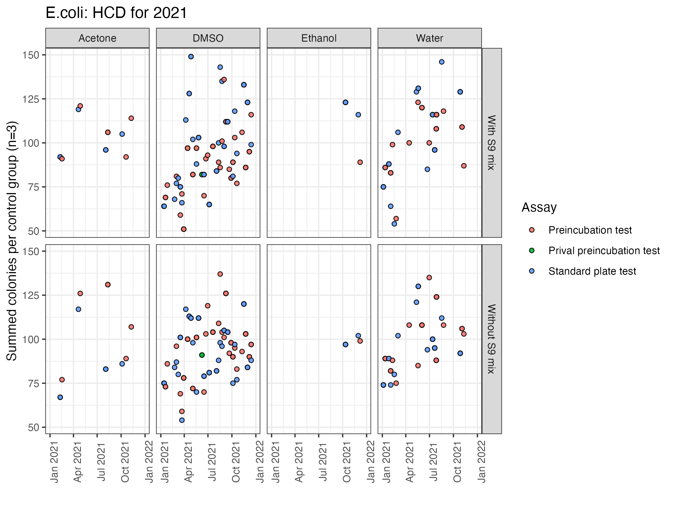
Figure 1: Overview about the number of revertant colonies in historical negative controls using E. coli (summed over three petri dishes per control group).

For a detailed analysis regarding the relationship between the mean and the variance, the historical data was split according to the different experimental setups (different combinations of bacteria stem, vehicle, S9 mix used or not used and type of assay). In order to assess these data sets for possible overdispersion, the model described in equations 4 and 5, was fitted to each of these data sets, if they contained at least five historical control groups (49 out of 90 data sets). This restriction was used, since the estimate for the dispersion parameter is slightly negatively biased and can be highly inaccurate, if estimated based on a small number of observations (McCullagh and Nelder 1989; Menssen and Schaarschidt 2019). The estimates for the dispersion parameter and the Poisson mean for each of these 49 data sets are depicted in figure 2.

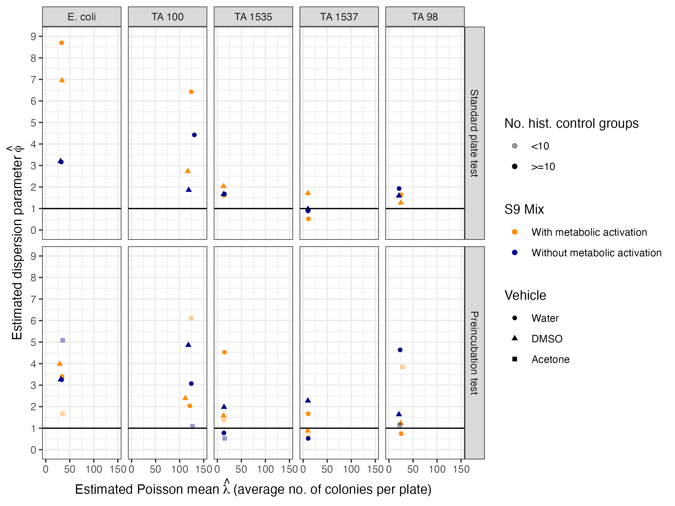
Figure 2: Overview about the estimates for the Poisson mean $\hat{\lambda}$ and the dispersion parameter $\hat{\phi}$ obtained from historical control data with at least five observations per setting.

It is apparent that most of the settings can be treated as overdispersed ($\hat{\phi}>1$). This means, that in this settings, the observed variability in the data exceeds the variability that can be modeled by the assumption of a simple Poisson process.
Especially for the bacteria stems E. coli and TA 100 the data is much more variable than under the assumption of simple Poisson distributed data, since the estimated dispersion parameter rises up to values above six. The most extreme case of overdispersion ($\hat{\phi}\approx 8.7$) was observed for E. coli in the standard plate test using S9 mix and water as the vehicle. Hence, in this data set the observed between study variability was modeled to be approximately 8.7 times higher, than possible under the assumption of simple Poisson distributed data.

4.2 Historical data about relapses of multiple sclerosis patients

Longitudinal data on the number of relapses of multiple sclerosis (MS) patients was provided by the German Multiple Sclerosis Registry (GMSR). This registry accumulates data from different types of health care centers (e.g. hospitals or medical practices that work with MS patients) across Germany through a certified web-based electronic data capture system. A wide range of variables such as demographical and clinical data are collected. Further details on the data collection of the GMSR can be found in Ohle et al. 2021.
In this work, the collected data of 36 different centers participating in the pharmacovigilance module of the GMSR were assessed in detail, out of which 21 were specialized centers that predominantly treat MS patients, while the other 15 centres are smaller and less focused on MS in the context of other neurological diseases. The data set contained observations from 1.1.2020 onwards until the last visit of each patient. The number of patients per center varied between 12 and 353 (fig. 3 A) whereas the observation period of those patients varied between 0.25 and 3.76 years (fig. 3 B). The number of patients within a center not having a documented relapse during the observation period varied between 25% and 99%.
In order to monitor the average relapse rate $\hat{\lambda}$ per patient per year and the between patient overdispersion $\hat{\phi}$ within each center, a GLM that was based on the quasi-Poisson assumption was fit to each of the 36 data sets (see computational details). Due to the relatively high number of zeros in some of the data sets, the average relapse rate per center $\hat{\lambda}$ can become relatively low and varies from 0.0032 to 0.426 (x-axis in figure 3 C). The estimated dispersion parameter per center $\hat{\phi}$ varied between 0.70 and 3.39 (y-axis in figure 3 C). Out of the 36 centers, 31 showed signs of slight to moderate overdispersion ($\hat{\phi}$ between 1.08 to 2.41), whereas five centers showed signs of underdispersion ($\hat{\phi}$ below 1).

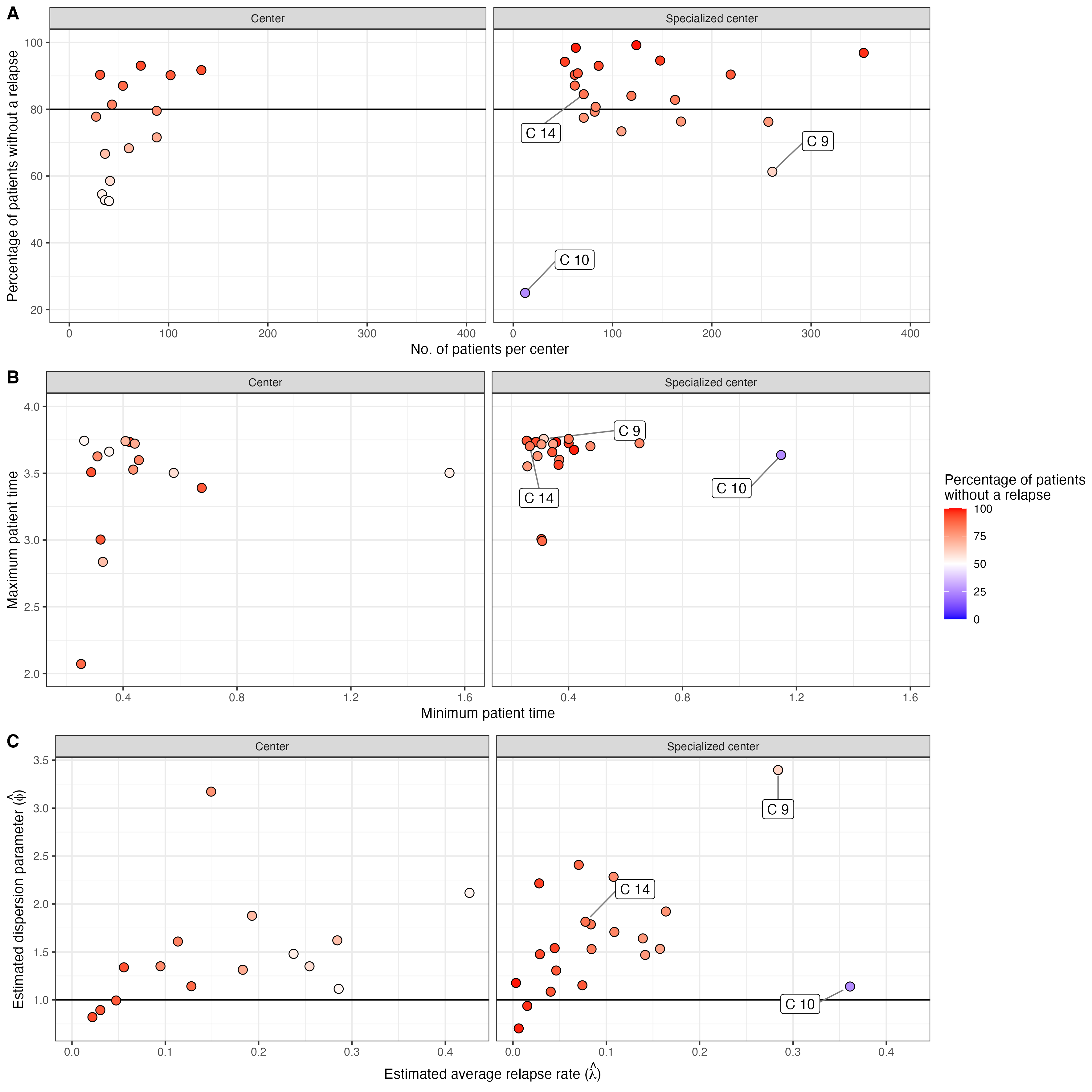
Figure 3: Overview on the data about the number of relapses per multiple sclerosis patient. A: Percentages of patients without any relapse per center. B: Minimum and maximum time patients are monitored by a certain center. C: Estimates for the Poisson mean $\hat{\lambda}$ (the average relapse rate per center and patient year) and the estimated dispersion parameter $\hat{\phi}$ per center. Centers 9, 10 and 14 are used in order to demonstrate the application of upper prediction limits (see section 6.2 below).

5 Simulation study

The coverage probabilities of the different methods for the calculation of HCL reviewed above were assessed by Monte-Carlo simulations with the nominal level set to $1-\alpha=0.95$. The simulation settings were inspired by the real life data shown above and some of the parameter combinations used for simulation reflect their properties. Nevertheless, simulations were run for a broader range of different parameter settings in order to enable a higher degree of generalization. Simulations were run for both, two sided control (or prediction) intervals (reflecting the settings in toxicology) as well as for one sided upper prediction bounds (reflecting the data properties in medical quality control).
For each combination of model parameters, $S=5000$ ”historical” data sets were drawn, on which historical control limits $[l,u]_{s}$ were calculated. Furthermore, $S$ sets of single target values $t^{*}_{s}$ (with $t^{*}=u^{*}=y^{*}/n^{*}$ for control limits in u-Charts and $t^{*}=y^{*}$ for all other control limits) were sampled and the coverage probability of the control intervals was computed by

$$\hat{\psi}^{cp}=\frac{\sum_{s=1}^{S}I_{s}}{S}\text{ with}$$

$$I_{s}=1\text{ if }t^{*}_{s}\in[l,u]_{s},$$

$$I_{s}=0\text{ if }t^{*}_{s}\notin[l,u]_{s}.$$

In order to assess the ability of the different historical control limits to ensure for equal tail probabilities (as was required in equation 7), the coverage of the simulated lower borders $l_{s}$ and upper borders $u_{s}$ was calculated to be

$$\hat{\psi}^{l}=\frac{\sum_{s=1}^{S}I_{s}}{S}\text{ with}$$

$$I_{s}=1\text{ if }l_{s}\leq t^{*}_{s},$$

$$I_{s}=0\text{ if }l_{s}>t^{*}_{s}.$$

and

$$\hat{\psi}^{u}=\frac{\sum_{s=1}^{S}I_{s}}{S}\text{ with}$$ (17)

$$I_{s}=1\text{ if }t^{*}_{s}\leq u_{s},$$

$$I_{s}=0\text{ if }u_{s}>t^{*}_{s}.$$

In the simulations regarding upper prediction limits that served as HCL, their coverage probability was calculated according to equation 17. Each of the bootstrap-calibrated prediction intervals (or upper limits) that were calculated in the simulation was based on $B=10000$ bootstrap-samples. The sampling of quasi-Poisson or negative-binomial observations was done following the algorithms described in section 4 of the supplementary material.

5.1 Coverage probabilities of two-sided historical control limits

In order to assess the coverage probability $\hat{\psi}^{cp}$ of the two HCL mentioned above, simulations for all 36 combinations of four different numbers of historical clusters $H=\{5,10,20,100\}$ that mimic different numbers of available historical control groups, three different Poisson means $\lambda=\{5,20,100\}$ and three different dispersion parameters $\phi=\{1.001,3,5\}$ were run. Reflecting the experimental design of toxicological studies, these parameter combinations were used in combination with offsets that remain constant between the historical clusters ($n_{h}=n^{*}=3$). Hence, in this part of the simulation, the mean-variance relationship of the quasi-Poisson assumption is not in contradiction with the one of the negative-binomial distribution.
The simulated coverage probabilities of the heuristical methods is given in figure 4 A whereas the coverage probabilities of the prediction intervals is given in figure 4 B. The control limits of the c- and u-charts behave similar: Both approach the nominal coverage probability of 95 % (red dots) if overdispersion does not play a role in the data, but show coverage probabilities far below the nominal level that decrease down to 58% in the presence of overdispersion (and hence are not depicted in the figure). The adjusted u-chart that accounts for overdispersion behaves in a similar way than the control limits given by the mean $\pm$ 2 standard deviations. With a rising number of historical control groups, both methods approach the nominal coverage probabilities. But, one has to be aware that both methods do not account for equal tail probabilities. Hence, their lower limits tend to cover the target value (one random realization of the data generating process) almost always, if the Poisson mean is low ($\lambda=5$) and overdispersion plays a role in the data ($\phi>1$), because in this case, the underlying distribution is heavily right-skewed.
The two simple (uncalibrated) prediction intervals (fig. 4 B) tend to behave in a similar fashion: They approach the nominal coverage probability if overdispersion plays only a minor role in the data, but yield coverage below the nominal level, if overdispersion plays a role and the number of historical control groups is below 20. Since these intervals do not account for equal tail probabilities, one has to be aware that they practically yield 95% upper prediction bounds in the case of a low Poisson mean and present overdispersion. This is due to the right-skeweness of the underlying distribution.
The calibrated prediction intervals tend to be slightly too conservative, if overdispersion is absent in the data and the number of historical studies is low. But, if the data is overdispersed the calibrated prediction intervals approach the nominal coverage probabilities, even if computed based on five historical control groups. Since the calibration algorithm is aimed to adapt the intervals to potential skewness of the underlying distribution, the lower and the upper borders of the calibrated prediction intervals approach the desired 97.5% coverage probability far closer than any other method.

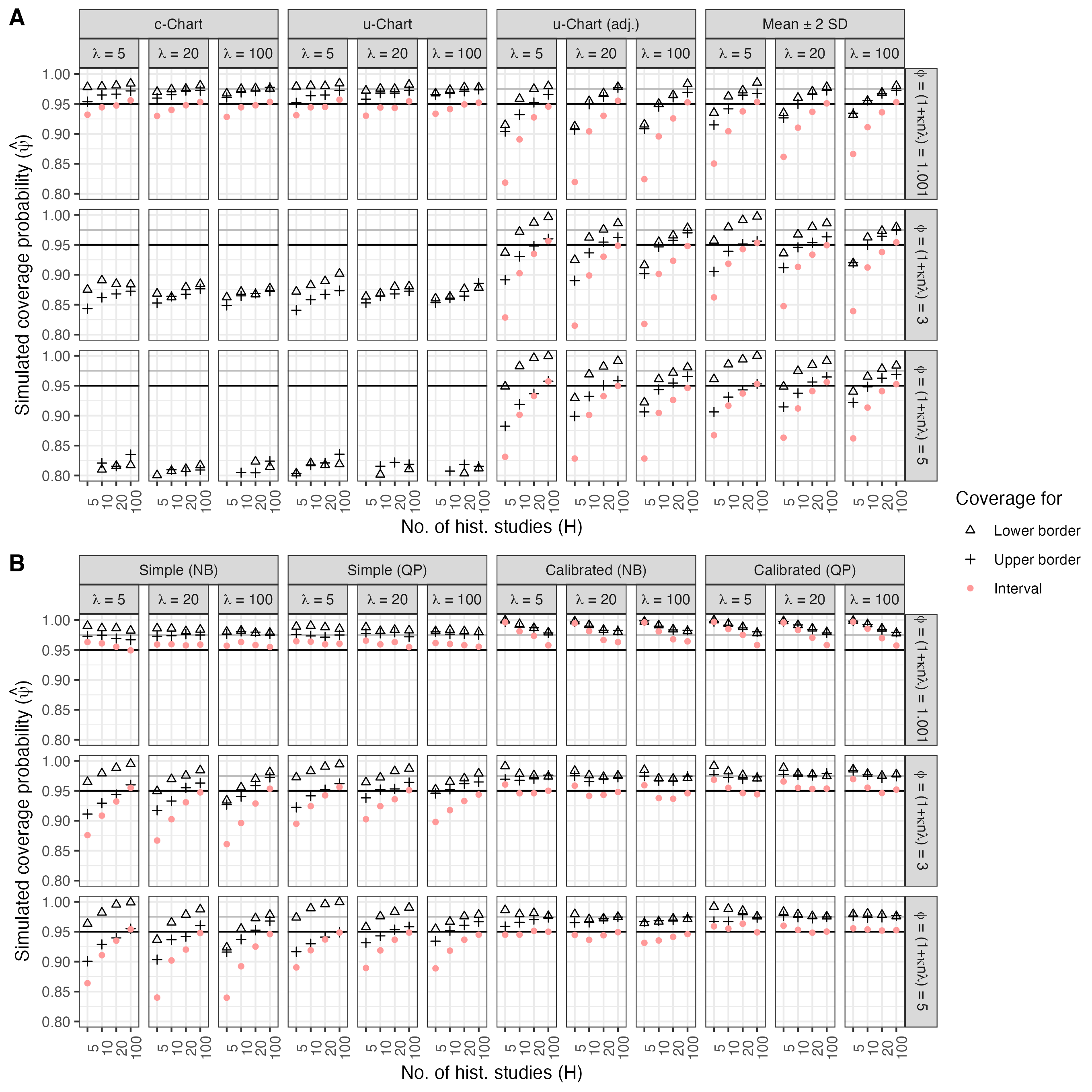
Figure 4: Simulated coverage probabilities based on $n_{h}=3$ experimental units per control group. A: Heuristical control limits. B: Prediction intervals. $\boldsymbol{\lambda}$: Poisson mean. Black horizontal lines: Nominal coverage probability $\psi^{cp}=0.95$. Grey horizontal line: Nominal coverage probability for the lower and the upper limit, if equal tail probabilities are achieved $\psi^{l}=\psi^{u}=0.975$

5.2 Coverage probabilities of calibrated upper prediction borders

This part of the simulation was run in order to reflect the application in medical quality control. Compared to toxicological applications, where the experimental setup is highly standardized with regard to the experimental design, genetic conditions of model organisms etc., medical data is usually derived from less controlled environments. Patients can differ greatly in age, genetic preposition and other risk factors which might lead to high degrees of possible overdispersion. Furthermore, the time patients spend under treatment (or in a hospital) can differ greatly between patients, which has to be taken into account for the application of control limits. Since medical quality control is usually applied in order to monitor the number of adverse events per patient the numbers of counted events is usually relatively low and therefore, can contain many zeros. But with an increasing amount of zeros in the data, the lower limit of control intervals turns out to be less informative (since it becomes zero itself). Hence, in this scenario the application of upper control limits has to be favored over the application of two sided control limits.
Since the bootstrap-calibrated prediction intervals outperformed all other methodologies in the simulation showed above, only bootstrap-calibrated upper prediction bounds are considered in this section. Monte-Carlo simulations regarding the coverage probability of the calibrated upper prediction limits were run based on all combinations of the following parameters $H=\{5,10,20,100\}$ mimicking the number of patients available for limit calculation, four different Poisson means $\lambda=\{0.1,1,5,20\}$ and four different amounts of overdispersion $\phi=\{1.001,3,5,10\}$.
In order to reflect the different patient times that were included as an offset ($n_{h}$ and $n^{*}$ in equations 15 and 16), offsets were sampled from a uniform distribution. In one step all 64 parameter combinations were simulated with offsets ranged between 0.5 and 4. This setting was chosen in order to reflect the patient times in the real life data from the GMSR. In order to evaluate the behavior of the prediction limits in the case were offsets are extremely different, all 64 parameter combinations were additionally run with offsets drawn from a uniform distribution with minimum 0.5 and maximum 50.
Quasi-Poisson data was sampled using the parameter combinations mentioned above. Based on this type of data, the coverage probabilities of both calibrated prediction limits (quasi-Poisson and negative-binomial) were assessed. Vice versa, observations were sampled from the negative-binomial distribution, to which both methods were applied. This was done in order to assess the performance of both methods under model misspecification.
As noted above, the mean-variance relationship differs between the quasi-Poisson assumption and the negative-binomial distribution in the case were offsets are different: In the negative-binomial distribution the Poisson variance is inflated by $1+\kappa n_{h}\lambda$ (see equation 5). Hence, contrary to quasi-Poisson data, the magnitude of overdispersion within each cluster (eg. patient) depends on the offset and is not a constant anymore. In order to set the amount of overdispersion in a comparable range as in the simulation based on quasi-Poisson data, the parameter $\kappa$ used for data sampling was set to $\kappa=\frac{\phi-1}{\bar{n}\lambda}$ with $\bar{n}=\{2.25,25.25\}$.
The simulated coverage probabilities are given in figures 5 and 6. Both methods yield coverage probabilities satisfactorily close to the desired 95% and seem to be relatively robust against model misspecification. However, all coverage probabilities are calculated based on the number simulated data sets to which a fitted model reached convergence. But, the negative-binomial GLM, fit with MASS::glm.nb, does not converge to a given data set in many cases. Especially with a rising amount of zeros ($\lambda=0.1$) and declining numbers of available patients ($H\leq 10$) the number of simulated data sets to which a negative-binomial GLM could be fit, became less than 50% and declined to a minimum of 24.5%. Contrary to the negative-binomial GLM, the GLM based on the quasi-Poisson approach did not show any problems with convergence, but yields estimates for the dispersion parameter $\hat{\phi}$ below one. Due to the necessity that $\hat{\phi}$ was restricted to be bigger than 1 in equations 13 and 15, the calibrated quasi-Poisson prediction interval is based on bootstrap data that was generated based on $\hat{\phi}=1.001$ if the true estimate was below one.

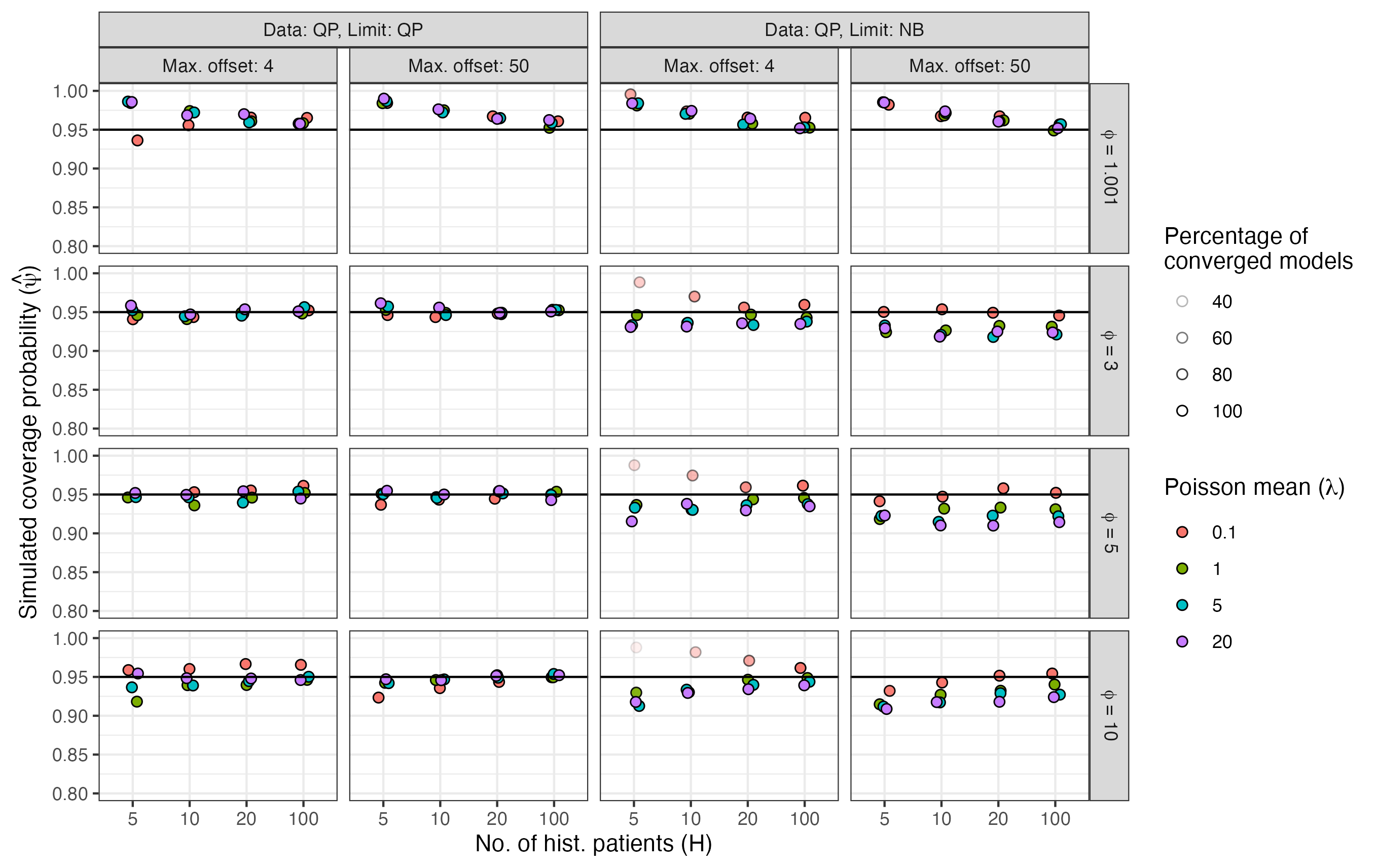
Figure 5: Simulated coverage probabilities of bootstrap-calibrated upper prediction limits based on quasi-Poisson data*. $\boldsymbol{\lambda}$: Poisson mean, $\boldsymbol{\phi}$: Dispersion parameter, Max. offset: Maximum offset used for simulation (the minimum offset was always fixed at 0.5), Black horizontal lines: Nominal coverage probability $\psi=0.95$, *All coverage probabilities were calculated based on the number of converged model fits.

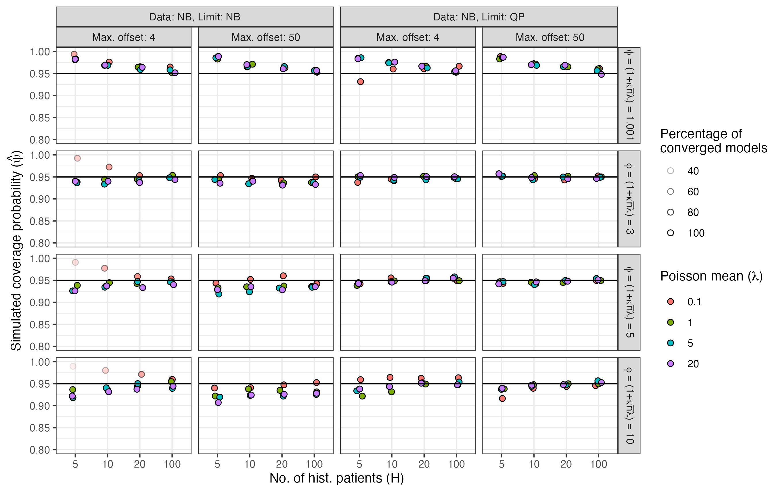
Figure 6: Simulated coverage probabilities of bootstrap-calibrated upper prediction limits based on negative-binomial data*. $\boldsymbol{\lambda}$: Poisson mean, $\boldsymbol{\phi}$: Dispersion parameter, Max. offset: Maximum offset used for simulation (the minimum offset was always fixed at 0.5), Black horizontal lines: Nominal coverage probability $\psi=0.95$, *All coverage probabilities were calculated based on the number of converged model fits.

6 Application of control limits

6.1 Pre-clinial risk assessment

In his paper from 1982, Tarone provided the results of a microbial mutagenicity assay run to evaluate the mutagenic potential of benz(a)anthracene, alongside with HCD that contains 66 control groups from similar mutagenicity assays. Each control group is comprised of three petri dishes on which the number of revertant bacteria colonies of the stem TA1537 was counted (tab. 2 and 3 of Tarone 1982). Since the number of petri dishes remains fixed for all control groups ($n_{h}=n_{h^{\prime}}=n^{*}=3$), one can not distinguish between the negative-binomial or quasi-Poisson assumptions. The estimated dispersion parameter is $\hat{\phi}=3.18$, which indicates that the variability of the data generating process from which the historical control groups derive is 3.18 times as variable as expected under simple Poisson distribution.
Different control limits calculated based on the HCD are depicted in table 1. The control limits from Sheward control charts (c- and u-Chart) yield the narrowest control intervals, since they ignore the overdispersion present in the HCD. If one multiplies its control limits by $n^{*}=3$, the overdispersion adjusted u-chart of Laney (2006) yields control limits that are comparable to the ones calculated based on the mean $\pm$ 2 SD as well as to the simple uncalibrated prediction intervals. This is because all four intervals are symmetrical and the amount of historical information is relatively high (and hence the uncertainty of the estimates used in the heuristical intervals is relatively low). The width of the two calibrated prediction intervals is comparable to the width of the uncalibrated ones. However, the control limits of the calibrated prediction intervals are systematically higher than the limits of the uncalibrated intervals. This is, because the calibration accounts for potential skeweness and hence yields non-symmetrical prediction intervals.

Table 1: Control limits for the number of revertant colonies in three petri dishes ($n^{*}=3$) based on the HCD given by Tarone 1982

Method	Lower CL	Upper CL	Interval width
c-Chart	15.25 (16)	34.87 (34)	19.62
u-Chart1	5.08 (6)	11.62 (11)	6.54
u-Chart (adj.)1	2.56 (3)	14.14 (14)	11.58
Mean $\pm$ 2 SD	7.20 (8)	42.92 (42)	35.72
Simple (NB)2	7.86 (8)	42.26 (42)	34.40
Simple (QP)3	7.43 (8)	42.70 (42)	35.27
Calibrated (NB)2	9.90 (10)	44.67 (44)	34.76
Calibrated (QP)3	9.70 (10)	45.16 (45)	35.46

Numbers in brackets: Lowest and highest number of counts covered by the interval.
1: Control limits of the u-Charts are given for $y^{*}/n^{*}$. For control limits on the response scale, multiply them by $n^{*}=3$.
2: Estimates $\hat{\lambda}=8.35$ and $\hat{\kappa}=0.082$ were obtained based on MASS::glm.nb (see computational details)
3: Estimates $\hat{\lambda}=8.35$ and $\hat{\phi}=3.18$ were obtained based on stats::glm (see computational details)

Since the calibrated prediction intervals account for the skeweness of the underlying distribution, they properly approximate the central $100(1-\alpha)$ % of the underlying distribution. Hence they can be applied in improved Sheward control charts. The left panel of figure 7 shows the HCD (grey dots), the expected number of revertant colonies $n\hat{\lambda}=25.06$ (black dashed line), the 95 % calibrated prediction interval (quasi-Poisson) given in table 1 (black lines) and a 99 % calibrated prediction interval based on the quasi-Poisson assumption $[l,u]=[6.36,54.64]$ (grey dashed lines). The right side of figure 7 shows the data of the current trial regarding benz(a)anthracene together with the 95 % prediction interval.
Based on the left panel, one can evaluate the quality of the HCD. Please note, that Tarone reported the HCD not as a timeseries, but rather reported the numbers of historical control groups in which a certain number of revertant colonies occurred. In order to demonstrate how a Sheward control chart would look like if the HCD was reported as a time series (which is usually the case), each control group was randomly assigned to an artificial study ID.
Based on this artificial study IDs, the process appears to be constant and most of the historical observations fall into the 95 % prediction interval with two values above the upper limit of the 95 % interval. But, given that there are 66 historical control groups, one can expect $66*0.05=3.3$ observations outside the central 95 % (and 0.66 outside the central 99 %).
If one compares the observations from the current trial to the HCD, it is apparent that the concurrent control group is relatively low, but all current observations seem to be in line with the historical ones. However, the prediction interval applied here has a pointwise interpretation and is explicitly based on the assumption, that only the concurrent control group is derived from the same data generating process as the historical controls.
It is important to note, that the evaluation, if the outcome of a complete current trial (control and treatment groups) is in line with the historical knowledge needs further adjustment to account for the multiple testing problem. Furthermore, due to systematic (but uncontrollable) differences between the different historical and current trials, all observations within a trial can be correlated (which causes the between study overdispersion). If these correlations play a role, the treatment groups can not be treated as independent realizations from the same data generating process the control groups are derived from. Hence, control limits that should evaluate a whole current trial have to be based on a simultaneous prediction interval, that accounts for possible within study correlation. To the authors knowledge, methodology to compute such a prediction interval is not available so far.

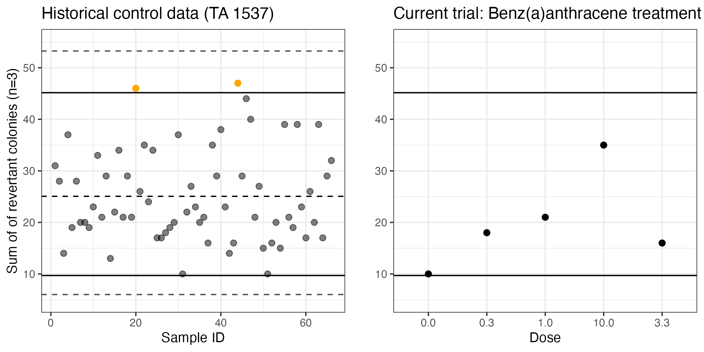
Figure 7: HCD and current trial of Tarone 1982. Black dashed line: Expected value for the number of revertant colonies in three petri dishes ($n\hat{\lambda}=25.06$), Black lines: Lower and upper border of the 95 % calibrated quasi-Poisson prediction interval (see tab. 1), Grey dashed lines: Lower and upper border of a 99 % calibrated quasi-Poisson prediction interval, Orange dots: Observations that fall outside 95 % prediction limits. Please note that the study ID is artificial.

6.2 Medical quality control

Contrary to toxicological HCD that usually contains observations which stem from control groups of controlled experiments run in a consecutive order, data for medical quality control is usually gathered on the levels of patients that randomly appear in health care centers. Hence, in medical quality control, a given sample of patients which represent the observations from a current process is taken as a baseline, to which patients from another cohort can be compared.
Three centers that report their data of MS patients to the GMSR serve as examples: Center 9, 10 and 14. Center 14 served as the reference based on which estimates for the average relapse rate and overdispersion were computed ($\hat{\phi}=1.81$, $\hat{\lambda}=0.077$). Together with individual patient times, these estimates were used to compute calibrated 95% and 99% upper prediction limits (UPL) for each patient within center 14. This was done to identify the patients that showed unusually high relapse rates and hence, might need clarification, if their high number of relapses is explainable by their course of the disease or possibly by a reporting error.
Compared to center 14, centers 9 and 10 report relatively high relapse rates (see fig. 3) and it is of interest, if both centers report data that is in line with center 14. Hence, UPL that were based on the estimates for the average relapse rate $\hat{\lambda}$ and the dispersion parameter $\hat{\phi}$ obtained in center 14 and the individual patient times observed in centers 9 and 10 were calculated to which the observed numbers of relapses were compared.
Table 2 provides an overview about the total number of patients per center, the percentage of patients that exceed a certain UPL as well as the corresponding observed vs. expected number of patients. For 21.45% of the patients in center 9, the number of relapses exceeds the 95% UPL (instead of the expected 5%). Furthermore, 2.3% of the patients have higher relapses than predicted by the upper 99% UPL. This clearly indicates, that in center 9 far more patients exceed the UPL as could be expected, if its underlying data generating process was in line with center 14. In other words: The unusual high numbers of relapses reported in center 9 can be interpreted as a warning signal, that systematic differences between center 14 and center 9 occur that need further investigation.
Similarly as in center 9, also in center 10 more patients than expected exceed the 95% UPL (3 out of 12), but none of the patients showed numbers of relapses above the 99% UPL. Given the low number of patients in center 10, this can be interpreted as a weak warning signal that the three patients need further investigation. But, it remains unclear, if the data generating process in center 10 really differs from the one in center 14.

Table 2: Percentage of patients per center, that exceed pointwise upper prediction limits

Center	$>$ 95% UPL	$>$ 99% UPL	N
C 14 (baseline)	2.82% (2, 3.55)	1.41% (1, 0.71)	71
C 9	21.45% (56, 13.05)	2.30% (17, 2.61)	261
C 10	25.00% (3, 0.6)	0.00% (0, 0.12)	12

Numbers in brackets: Observed vs. expected numbers of patients with relapses above the control limit. UPL: Upper prediction limit. N: Total number of patients per center.

Sheward type control charts, that are based on the calculated UPL are depicted in fig. 8. In order to keep patients unidentifiable, 10 patients with a maximum of 4 relapses were randomly chosen from each center.
The expected number of relapses per patient as well as individual 95% and 99% UPL are indicated by the dashed, the black and the grey lines, respectively. The different width of the UPL reflects the different times patients have spent under monitoring. Orange dots indicate patients above the 95% UPL whereas red dots indicate patients that belong to the one percent with the highest relapse rates (given that they would originate from the same data generating process as the patients in center 14). As stated above, far more patients than expected exceed the UPL in center 9. This can be interpreted as a warning signal that the whole data generating process of center 9 differs from that in center 14.
Beyond that, the Sheward type control chart given in fig. 8 is a relatively simple tool to detect single patients that show an unusual high number of relapses and hence need further investigation: Since patient 9 of center 9 has spent a relatively short time under monitoring, also its UPL are relatively low. Consequently, the four relapses of this patient would belong to the most extreme 1%, if this patient was prone to the same data generating process than the patients in center 14 and hence, needs further investigation.

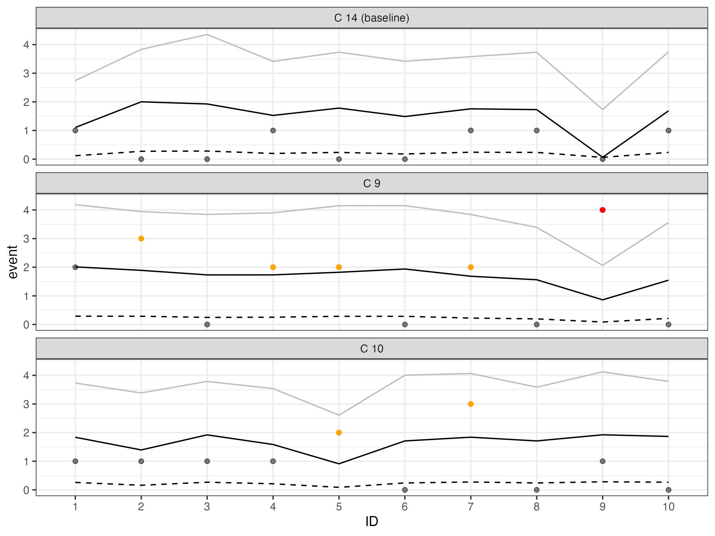
Figure 8: Control-chart for the number of relapses for 10 random MS patients per center. Dashed line: Expected number of relapses per patient, Black line: Calibrated 95 % upper prediction limits (quasi-Poisson)*, Grey line: Calibrated 99 % upper prediction limits (quasi-Poisson)*, Grey dots: Observed number of relapses per patient, Orange dots: Observed numbers of relapses per patient exceeds 95 % upper prediction limit, Red dots: Observed numbers of relapses per patient exceeds 95 % upper prediction limit, * All limits are calculated based on estimates ($\hat{\lambda}=0.077$ and $\hat{\phi}=1.81$) obtained from center 14.

7 Discussion

The analysis of the two real life data bases provides evidence for the presence of overdispersion in toxicological and medical count data. The amount of overdispersion found in the HCD that descends from the Ames test is in line with the findings of others: Obviously the HCD provided by Tarone 1982, that was used in section 6.1 as an example for the application of the proposed methodology, shows clear signs of overdispersion. Furthermore, Levy et al. 2019 report HCD from negative control groups about the Ames test that was provided by more than 20 different laboratories, summarized in 18 different data sets. However, they report the HCD in terms of means and standard deviations (per data set). If one squares their reported standard deviations and compares the resulting variances to the reported means, the variance exceeds the mean in 12 out of 18 of data sets. With other words, also this 12 data sets contain observations of different historical negative control groups that show signs of between study overdispersion.
The presence of overdispersion in the registry data is in line with medical and biopharmaceutical data reported by others: Mohammed et al. 2008 reported a data set on the number of falls per patient in a hospital department for which, based on the quasi-Poisson assumption, the estimated amount of overdispersion is $\hat{\phi}=1.67$. Hoffman 2003 reported a data set on bacteria counts in water probes that appeared to be heavily overdispersed ($\hat{\phi}=9.38$).
This demonstrates the need for methodology that enables the calculation of historical control limits for overdispersed count data. Unfortunately the existing methodology for the calculation of HCL for count data has several drawbacks: All of them are based on heuristics that formally lack a clear definition of their statistical properties (since they lack a formal definition for the desired coverage probability). Furthermore, they yield HCL symmetrical around the mean, but overdispersed count data can be heavily right skewed (see fig. 1 in the supplementary material). Consequently all heuristical methods, reviewed above do not ensure for equal tail probabilities and they are not able to approximate the central $100(1-\alpha)$% of the underlying distribution.
This gap was closed by the proposed bootstrap calibrated prediction intervals. Even for a relatively low number of historical clusters (e.g. control groups or patients) the bootstrap calibration yields prediction intervals (or limits) with coverage probabilities close to the nominal level. Since the proposed procedure calibrates the lower and the upper limits individually, the resulting prediction interval reflects the skeweness of the underlying distribution and hence, ensures for equal tail probabilities.
Despite the fact that overdispersion is present in toxicological and medical real life data and the proposed prediction intervals are able to care about overdispersion, its presence indicates that some sources of variability are not uniform between historical clusters. Especially in toxicological applications, where HCD stems from controlled experiments, the presence of overdispersion should trigger a closer look to the historical control data base in order to search for potential systematic sources for between study variation that can be controlled. On the other hand overdispersion is a common feature of biological count data (McCullagh and Nelder 1989) because living experimental units can only be standardized up to a certain level (e.g. with regard to their genetic condition or age).
Therefore the presence of overdispersion might reflect a mixture of controllable and uncontrollable sources for between study variability. Due to the possibility, that between study overdispersion can be caused by a mixture of different sources of which some might be controllable and others are not, a clear statement on the tolerable magnitude of between study overdispersion can not be given here. This must be subject to the toxicological research community and needs assay specific discussions.

8 Conclusions

If overdispersion is present in the data (and its magnitude is tolerable):

• Common Sheward c- and u-charts do not account for possible right-skeweness of the data. Therefore, more observations than desired will fall above the upper limit whereas fewer observations than desired will fall below the lower limit.

• The bootstrap calibrated prediction intervals yield coverage probabilities close to the nominal level. Furthermore, they account for equal tail probabilities and hence, should be favored over all other methods reviewed in this manuscript.

• Software for the calculation of bootstrap calibrated prediction intervals is publicly available via the R package predint.

9 References

Benoit S.W., Goldstein S.L., Dahale D.S., Haslam D.B., Nelson A., Truono K., Davies S.M. (2019): Reduction in Nephrotoxic Antimicrobial Exposure Decreases Associated Acute Kidney Injury in Pediatric Hematopoietic Stem Cell Transplant Patients. Biology of Blood and Marrow Transplantation 25:1654-1658

Chen T-T., Chung K-P., Hu F-C., Fan C-M., Yang M-C. (2010): The use of statistical process control (risk-adjusted CUSUM, risk-adjusted RSPRT and CRAM with prediction limits) for monitoring the outcomes of out-of-hospital cardiac arrest patients rescued by the EMS system. Journal of Evaluation in Clinical Practice 17:71–77

Coja T., CharistouA., Kyriakopoulou A., Machera K., Mayerhofer U., Nikolopoulou D., Spilioti E., Spyropoulou A., Steinwider J., Tripolt T. (2022): Preparatory work on how to report, use and interpret historical control data in (eco)toxicity studies. EFSA Supporting Publications 19(9):7558E

Demetrio C.G.B., Hinde J. ,Moral R.A. (2014): Models for overdispersed data in entomology. In: Ferreira C.P., Godoy W.A.C. (eds.) Ecological modelling applied to entomology. Springer International Publishing 219-259

Dertinger S. D., Li D., Beevers C., Douglas G.R., Heflich R.H., Lovell D.P., Roberts D.J., Smith R., Uno Y., Williams A., Witt K.L., Zeller A., Zhou C. (2023): Assessing the quality and making appropriate use of historical negative control data: A report of the International Workshop on Genotoxicity Testing (IWGT). Environmental and Molecular Mutagenesis 1-22

Deschl U., Kittel B., Rittinghausen S., Morawietz G., Kohler M., Mohr U., Keenan C. (2002): The Value of Historical Control Data - Scientific Advantages for Pathologists, Industry and Agencies. Toxicologic Pathology 30(1):80-87

EU Comission Regulation 283/2013: Setting out the data requirements for active substances, in accordance with Regulation (EC) No. 1107/2009 of the European Parliament and of the Council concerning the placing of plant protection products on the market.

Francq B.G., Lin D., Hoyer W. (2019): Confidence, prediction, and tolerance in linear mixed models. Statistics in Medicine 38:5603–5622

Greim H., Gelbke H-P., Reuter U., Thielmann H.W., Edler L. (2003): Evaluation of historical control data in carcinogenicity studies. Human and Experimental Toxicology 22:541-549

Gsteiger S., Neuenschwander B., Mercier F., Schmidli H. (2013): Using historical control information for the design and analysis of clinical trials with overdispersed count data. Statistics in Medicine 32:3609–3622

Gurjanov A., Kreuchwig A., Steiger-Hartmann T., Vaas L.A.I. (2023): Hurdles and signposts on the road to virtual control groups—A case study illustrating the influence of anesthesia protocols on electrolyte levels in rats. Fronties in Pharmacology 14:2023

Hahn G.J., Meeker W.Q. (1991): Statistical Intervals: A Guide for Practitioners. First edition, Wiley NY

Hayashi M., Dearfield K., Kasper P., Lovell D., Martus H-J., Thybaud V. (2011): Compilation and use of genetic toxicity historical control data. Mutation Research/Genetic Toxicology and Environmental Mutagenesis 723:87–90

Hoffman D. (2003): Negative binomial control limits for count data with extra Poisson variation. Pharmaceutical Statistics 2:127–132

Hoffman D., Berger M. (2011): Statistical considerations for calculation of immunogenicity screening assay cut points. Journal of Immunological Methods 373:200–208

Hothorn L.A. 2015: Statistics in Toxicology Using R. Chapman and Hall

Kluxen F.M., Weber K., Strupp C., Jensen S.M., Hothorn L.A., Garcin J-C., Hofmann T. (2021): Using historical control data in bioassays for regulatory toxicology. Regulatory Toxicology and Pharmacology 125:105024

Koetsier A., van der Veer S.N., Jager K.J., Peek N., de Keizer N.F. (2012): Control Charts in Healthcare Quality Improvement. Methods of information on Medicine 51(3):189-198

Levy D.D., Zeiger E., Escobar P.A., Hakura A., van der Leede B-J. M., Kato M., Moore M.M., Sugiyama K-I. (2019): Recommended criteria for the evaluation of bacterial mutagenicity data (Ames test). Mutation Research/Genetic Toxicology and Environmental Mutagenesis 848:403074

Lyren A., Brilli R.J., Zieker K., Marino M., Muenthing S., Sharek P.J. (2017): Children’s Hospitals’ Solutions for Patient Safety Collaborative Impact on Hospital-Acquired Harm. Pediatrics 140(3):e20163494

McCullagh P., Nelder J.A. (1989): Generalized Linear Models. 2nd Edition, Chapman and Hall

Meeker W.Q., Hahn G.J., Escobar L.A. (2017): Statistical Intervals: A Guide for Practitioners and Researchers, 2nd Edition, Wiley

Menssen M. 2023: The calculation of historical control limits in toxicology: Do’s, don’ts and open issues from a statistical perspective. Mutation Research/Genetic Toxicology and Environmental Mutagenesis 892:503695

Menssen M., Schaarschmidt F. (2019): Prediction intervals for overdispersed binomial data with application to historical controls. Statistics in Medicine 38(14):2652-2663

Menssen M., Schaarschmidt F. (2022): Prediction intervals for all of M future observations based on linear random effects models. Statistica Neerlandica 76(3)283-308

Mohhamed M.A., Worthington P., Woodall W.H. (2008): Plotting basic control charts: tutorial notes for healthcare practitioners. Quality and Safety in Health Care, 17(2):137-4

Montgomery D.C. (2020): Introduction to statistical quality control. Wiley, Hoboken NY

Nelson W. (1982): Applied Life Data Analysis. Wiley NY

NTP (2024): NTP Historical Controls Data Base. https://ntp.niehs.nih.gov/data/controls, assessed 2.2.2024

OECD (2017): Overview on genetic toxicology TGs, OECD Series on Testing and Assessment, No. 238, OECD Publishing, Paris

OECD (471): Test No. 471: Bacterial Reverse Mutation Test. OECD Guidelines for the Testing of Chemicals, Section 4, OECD Publishing, Paris

OECD (489): Test No. 489: In Vivo Mammalian Alkaline Comet Assay. OECD Guidelines for the Testing of Chemicals, Section 4, OECD Publishing, Paris

OECD (490): Test No. 490: In Vitro Mammalian Cell Gene Mutation Tests Using the Thymidine Kinase Gene. OECD Guidelines for the Testing of Chemicals, Section 4, OECD Publishing, Paris

Ohle LM., Ellenberger D., Flachenecker P. Friede T., Haas J., Hellwig K., Parciak T., Warnke C., Paul F., Zettl U.K., Stahlmann A. (2021): Chances and challenges of a long-term data repository in multiple sclerosis: 20th birthday of the German MS registry. Scientific Reports 11:13340

Pognan F., Steger-Hartmann T., Díaz C., Blomberg N., Bringezu F., Briggs K., Callegaro G., Capella-Gutierrez S., Centeno E., Corvi J., Drew P., Drewe W.C., Fernández J.M., Furlong L.I., Guney E., Kors J.A., Mayer M.A., Pastor M., Piñero J., Ramírez-Anguita J.M., Ronzano F., Rowell P., Saüch-Pitarch J., Valencia A., van de Water B., van der Lei J., van Mulligen E., Sanz F. (2021): The eTRANSAFE Project on Translational Safety Assessment through Integrative Knowledge Management: Achievements and Perspectives. Pharmaceuticals (Basel) 14(3):237.

Prato E., Biandolino F., Parlapiano I., Grattagliano A., Rotolo F., Buttino i. (2023): Historical control data of ecotoxicological test with the copepod Tigriopus fulvus. Chemistry and Ecology 39(8):881-893

Rotolo F., Vitiello V., Pellegrini D., Carotenuto Y., Buttino I. (2021): Historical control data in ecotoxicology: Eight years of tests with the copepod Acartia tonsa. Environmental Pollution. 284:117468

Sachlas A., Bersimis S., Psarakis S. (2019): Risk-Adjusted Control Charts: Theory, Methods, and Applications in Health. Statistics in Biosciences 11:630–658

Schaarschmidt F., Hofmann M., Jaki T., Gruen B., Hothorn L.A. (2015): Statistical approaches for the determination of cut points in anti-drug antibody bioassays. Journal of Immunological Methodsm 418:84–100

Still M.D., Cross L.C., Dunlap M., Rencher R., Larkins E., Carpener D.L., Buchmann T.G., Coopersmith C.M. (2013): The Turn Team: A Novel Strategy for Reducing Pressure Ulcers in the Surgical Intensive Care Unit. Journal of the American College of Surgeons 216(3):373-37

Tejs S. (2008): The Ames test: a methodological short review. Environmental Biotechnology 4(1):7-14

Viele, K., Berry, S., Neuenschwander, B., Amzal, B., Chen, F., Enas, N., Hobbs, B., Ibrahim, J.G., Kinnersley, N., Lindborg, S., Micallef, S., Roychoudhury, S. and Thompson, L. (2014): Use of historical control data for assessing treatment effects in clinical trials. Pharmaceutical Statistics 13:41-54.