Constructing Data Transaction Chains Based on Opportunity Cost Exploration

Abstract.

Data trading is increasingly gaining attention. However, the inherent replicability and privacy concerns of data make it challenging to directly apply traditional trading theories to data markets. This paper compares data trading markets with traditional ones, focusing particularly on how the replicability and privacy of data impact data markets. We discuss how data’s replicability fundamentally alters the concept of opportunity cost in traditional microeconomics within the context of data markets. Additionally, we explore how to leverage this change to maximize benefits without compromising data privacy. This paper outlines the constraints for data circulation within the privacy domain chain and presents a model that maximizes data’s value under these constraints. Specific application scenarios are provided, and experiments demonstrate the solvability of this model.

1. Introduction

Over the past few decades, the pricing and trading of the data, as well as the associated trading markets, have experienced rapid development. There have been many relevant research results, see (Zhang et al., 2023; Pei, 2020).

The design of market mechanisms for data trading is one of the popular research directions recently, with an increasing number of studies focusing on this area. Unlike traditional market trading, the data elements can be replicated at a low cost and the privacy of the data elements need to be protected. It leads to traditional trading mechanisms being impossible to fully graft onto the data transactions. In (Agarwal et al., 2019), the authors introduce an effective data trading mechanism, which gives the strategies for matching buyers and sellers as well as how the market interacts. Additionally, the authors present a robust-to-replication algorithm, ensuring that even if the traded data is replicated, it will not affect its market pricing. In (Chen et al., 2022), the authors introduce another data trading mechanism to prevent the devaluation of the seller’s data after replication. This method involves the seller initially presenting a portion of the data to the buyer as sample data along with a selling price. Then the buyer conducts Bayesian inference to predict the accuracy and quality of the data via the corresponding prior knowledge, thus determining whether to purchase the data at the offered price or not. In terms of privacy protection, (Amiri et al., 2023) presents a trading mechanism that not only protects data privacy but also allows the seller to demonstrate the quality of the data to the buyer. In this paper, the quality of the data depends on the relevance of the sold data to the buyer’s needs. This mechanism incorporates the traditional privacy protection method, i.e., principal component analysis, see also (Mangoubi et al., 2022; Leake et al., 2021).

The valuation of data points, which involves assessing and ranking the importance of each data point within a dataset, is also a crucial aspect of data trading. The most classic data valuation method is the Shapley value method from traditional game theory(Jia et al., 2019; Ghorbani and Zou, 2019), i.e., viewing each data point as a cooperating member, the importance of each data point is evaluated based on the trained model accuracy. We refer to the Shapley value method in Section 5. In (Wang et al., 2020), the authors proposed a valuation algorithm that combines the Shapley value with federated learning. In this case, federated learning ensures data privacy on the client servers, while Shapley value calculation guarantees fairness in data valuation.

We consider the transaction process on a data chain. In (Karlaš et al., 2022), the authors present a data valuation algorithm for assessing the value of each data point at different positions in the data processing chain. The advantage of this algorithm is that the authors no longer focus on a single model training scenario, but rather separate the modeling process for discussion. In (Yu et al., 2023), the authors model the transaction process between nodes as a Markov decision process and use reinforcement learning algorithms for multiple transactions to find the optimal data pricing mechanism.

Our contribution There has been fruitful research on the design of data trading market mechanisms and the valuation of data and models. However, most of them overlook the differences between the data trading market and the traditional trading market, which are influenced by data replicability and privacy, and due to these differences, how to construct models to maximize the benefits for the supply-side nodes. We give two main aspects in this paper. Firstly, the trading field of the data is limited by the privacy. Also, we consider the data trading path to be chain-like in this paper. Due to the replicability, for each node on the data chain, selling the training model to the market, and selling the data itself to the downstream node, which is then used by the downstream node to train the model for sale to the market, are not mutually exclusive. It leads to differences in the opportunity cost of data transactions compared to the opportunity cost proposed in classic microeconomic theory. To the best of our knowledge, we are the first to discuss the opportunity cost in data transactions.

2. Motivation

In microeconomic theory, the concept of opportunity cost is a prevalent notion. It reveals the value that is given up in order to obtain the higher value from the selected opportunity, see (Buchanan, 1991).

We consider the opportunity cost in the traditional industry. The seller has several options to make a profit, such as selling the product directly to the market, or reprocessing the product to obtain a higher unit price and then selling it to the market, along with other options within legal and other limitations, see Figure  1. Rational sellers will always choose the option with the highest total revenue, and the next best alternative not chosen represents the corresponding opportunity cost.

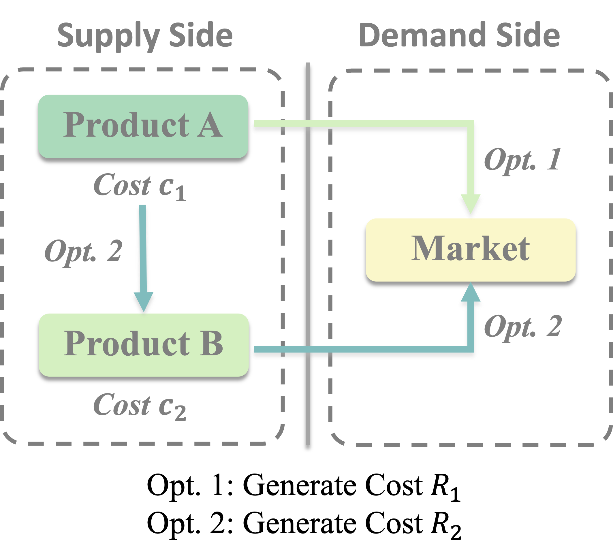
Figure 1. Traditional Industrial Scene

In the data transaction, such a trade-off naturally exists. However, unlike traditional scenarios, data has two distinctive characteristics, replicability and privacy. The replicability determines that some transaction options are not mutually exclusive. For instance, sellers can both sell the data to others and train the model by themselves at the same time. Selling data to others will result in multiple models based on the same dataset being sold in the market subsequently, and leads to competition. At this point, the seller chooses between two options: directly training models for sale or selling the data to others while simultaneously training models for sale, see Figure  2. The option not chosen represents the corresponding opportunity cost.

Privacy determines that it is also necessary to consider the privacy protection of the data in the transaction. For instance, it is not allowed to sell the data to the market directly even if it generates more revenue, since it leads to data privacy leakage.

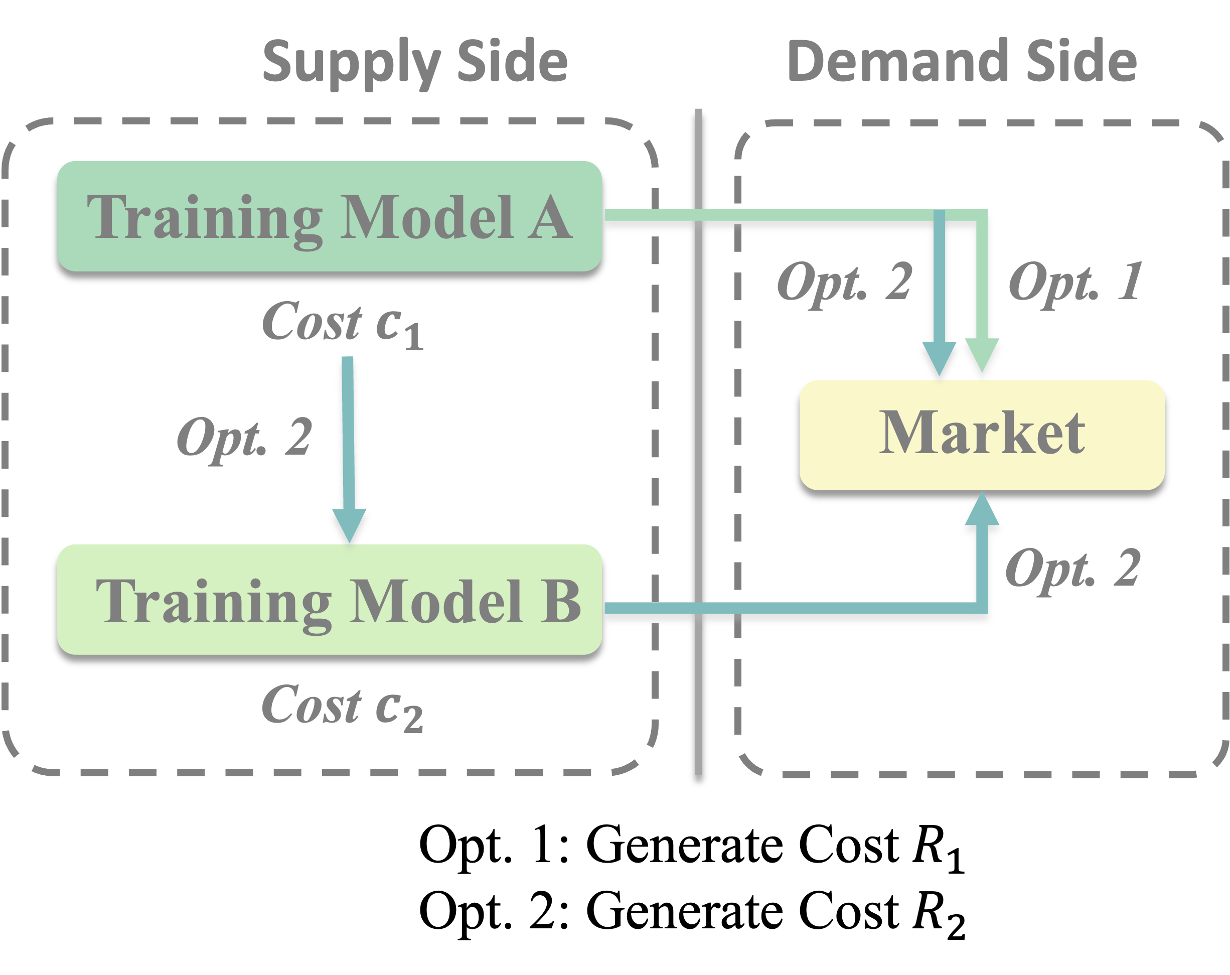
Figure 2. Data Trading Market Scene

Remark 2.1.

In this paper, we assume the privacy of the data must not be compromised in any way. However, in practical scenarios, such as in communication contexts, this condition may not be entirely achievable. In (Shokri et al., 2012), the authors present a strategy for customers to obtain more accurate services by disclosing partial location privacy to the service provider. Moreover, the customers’ disclosure of one-unit privacy in exchange for a one-unit improvement in service is referred to as the shadow price of service.

Remark 2.2.

In the data transaction situation, the data can be directly traded within the scope of privacy permissions, or it can be used to train and trade models afterward. Also, both the circulation of data itself and the circulation of models coexist. Then it is hard to distinguish the supply-side and the demand-side. In this paper, for a fixed dataset $D$, we define the supply-side as the field that allows data to circulate directly, and we define the demand-side as the field that can only purchase the trained models.

3. Modeling

In this paper, we focus on designing a mechanism for a data transaction chain to maximize the total revenue, see Figure  3.

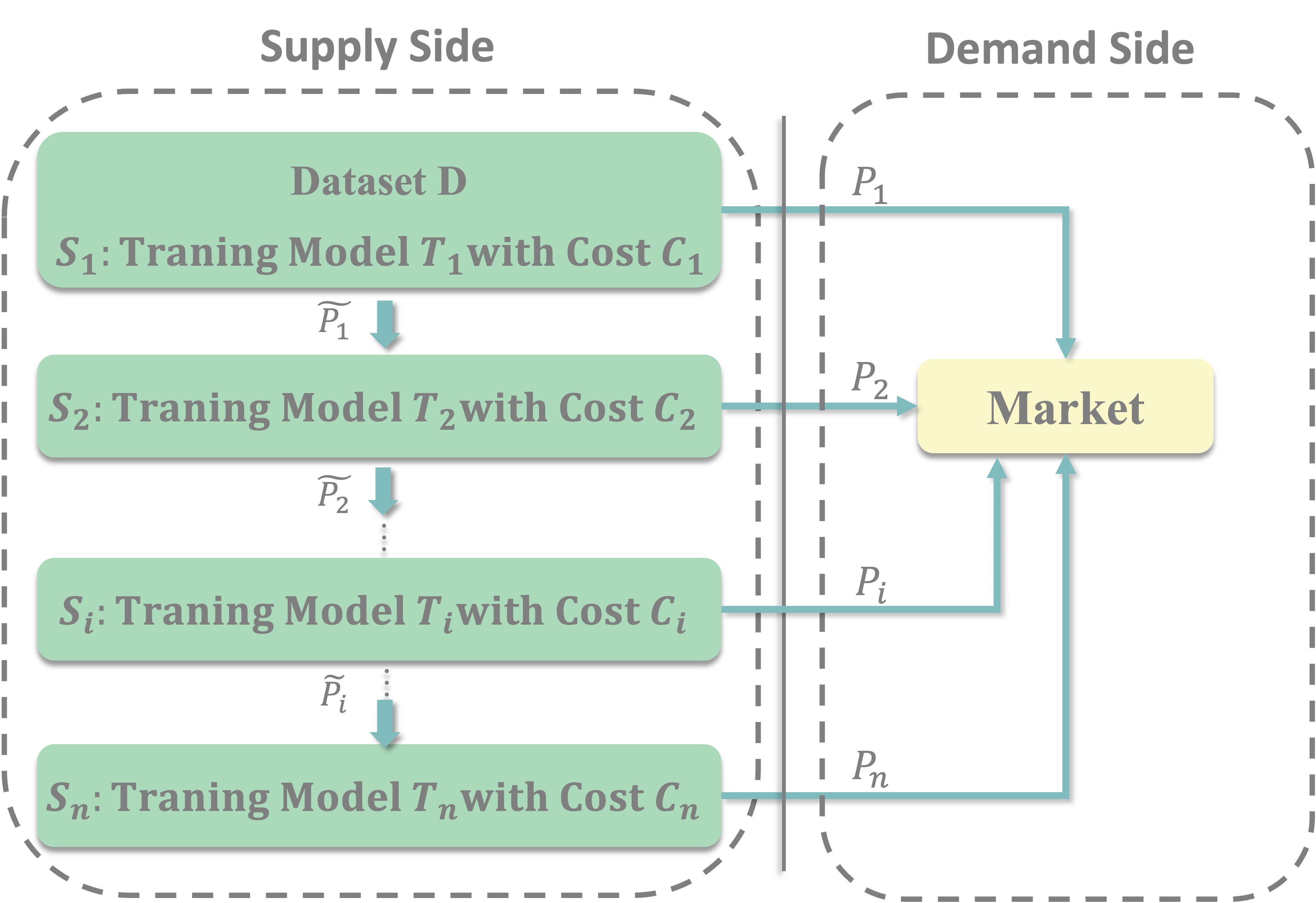
Figure 3. Data Trading Process (Dataset D cannot be directly sold to the market)

Let $\mathbb{S}:s_{1}\to s_{2}\to\cdots\to s_{n}$ be a data transaction chain, and initially, the node $s_{1}$ possesses a dataset $D$. The notations we use are shown in Table 1.

Table 1. Notations

$\mathbb{S}$	Data transaction chain
$s_{i}$	The $i$-th node
$T_{i}$	The model trained by $s_{i}$
$r_{i}$	Sales volume of $T_{i}$ in the market
$p_{i}$	Unit price of $T_{i}$
$c_{i}$	Cost for training $T_{i}$
$\tilde{p}_{i}$	Price where the node $s_{i}$ sells $D$ to $s_{i+1}$
$\delta_{i}$	Discount factor of $T_{i}$

There are two options for $s_{1}$ making profits, i.e., training and selling model $T_{1}$ to market and selling dataset $D$ to $s_{2}$. The revenue with the transaction not happening of node $s_{1}$ is $r_{1}p_{1}-c_{1}$. Also, the revenue with the transaction is $\tilde{p}_{1}+\delta_{1}r_{1}p_{1}-c_{1}$. The transaction happens only if the node $s_{1}$ obtains higher revenue, i.e.,

$$r_{1}p_{1}-c_{1}\leq\tilde{p}_{1}+\delta_{1}r_{1}p_{1}-c_{1}.$$

In $s_{2}$’s perspective, the trading between $s_{1}$ and $s_{2}$ happens if and only if the revenue surpasses the cost, i.e.,

$$r_{2}p_{2}-\tilde{p}_{1}-c_{2}\geq 0.$$

The transaction between $s_{1}$ and $s_{2}$ happens if and only if the solution set of $\tilde{p}_{1}$ is non-empty, i.e.,

$$r_{1}p_{1}-\delta_{1}r_{1}p_{1}\leq r_{2}p_{2}-c_{2}.$$

Similarly, the trading between $s_{i}$ and $s_{i+1}$ happens if and only if, in $s_{i}$’s perspective, the revenue with trading happening exceeds the revenue without trading happening, i.e.,

$$r_{i}p_{i}-c_{i}-\tilde{p}_{i-1}\leq\tilde{p}_{i}+\delta_{i}r_{i}p_{i}-c_{i}-\tilde{p}_{i-1}$$

and in $s_{i+1}$’s perspective, the revenue surpasses the cost, i.e.,

$$r_{i+1}p_{i+1}-c_{i+1}-\tilde{p}_{i}\geq 0.$$

In this case, the transaction between $s_{i}$ and $s_{i+1}$ happens if and only if the solution set of $\tilde{p}_{i}$ is non-empty, i.e.,

(1) $$r_{i}p_{i}-\delta_{i}r_{i}p_{i}\leq r_{i+1}p_{i+1}-c_{i+1}.$$

Remark 3.1.

We give an alternative perspective on this mechanism. From the inter-node transaction’s perspective, (1) provides a necessary and sufficient condition for this transaction to be achieved. Moreover, after re-arranging (1), we have

$$c_{i+1}\leq r_{i+1}p_{i+1}+\delta_{i}r_{i}p_{i}-r_{i}p_{i}.$$

It mentions that, from the data transaction chain’s perspective, the necessary and sufficient condition for dataset $D$ flowing in this arrow is that the difference in profit between node trading and non-trading can cover the downstream node’s model training cost.

Now we give the model. Our goal is to maximize the total revenue within the constraints of $c_{i}$($i=1,2,\ldots,n$). Also, we need to add the constraints that the trade between $s_{i}$ and $s_{i+1}$ happens. We have

(2) $$\max\underset{i=1}{\stackrel{{\scriptstyle n}}{{\sum}}}r_{i}\delta_{i}p_{i}$$

$$r_{i}p_{i}-\delta_{i}r_{i}p_{i}\leq r_{i+1}p_{i+1}-c_{i+1},\quad i=1,2,\ldots,n-1$$

$$\delta_{n}=1$$

$$\text{constraints of }c_{i}\text{'s}.$$

Remark 3.2.

In the previous context, we assume that the training of models in downstream nodes depends on the training results of upstream nodes, meaning that all nodes involved in the data transaction train the data. However, there is another possible scenario in real-world settings that, upstream nodes can choose to sell data directly to downstream nodes. Additionally, downstream model training relies solely on the data itself rather than the training results of upstream nodes. In this case, upstream nodes can assess whether the revenue for selling the model can cover the training cost if they sell the data to downstream nodes simultaneously. The corresponding programming is

$$\max\underset{i=1}{\stackrel{{\scriptstyle n}}{{\sum}}}r_{i}\delta_{i}p_{i}$$

$$r_{i}p_{i}-c_{i}-\max\{\delta_{i}r_{i}p_{i}-c_{i},0\}\leq r_{i+1}p_{i+1}-c_{i+1},\quad i=1,2,\ldots,n-1$$

$$\delta_{n}=1$$

$$\text{constraints of }c_{i}\text{'s}.$$

Remark 3.3.

In some cases, $r_{i}$ can be reflected as a function of the cost $c_{i}$, since both $r_{i}$ and $c_{i}$ are related to the model $T_{i}$’s accuracy $a_{i}$. We define

$$r_{i}=f_{i}(E[a_{i}|c_{i}]).$$

Also, by Bayesian inference, we have

$$Pr(a_{i}|c_{i})=\frac{Pr(a_{i},c_{i})}{Pr(c_{i})}=\frac{Pr(c_{i}|a_{i})\mu_{i}(a_{i})}{\sum_{a_{i}}Pr(c_{i}|a_{i})\mu_{i}(a_{i})}.$$

It leads to

$$E[a_{i}|c_{i}]=\sum_{a_{i}}a_{i}\frac{Pr(c_{i}|a_{i})\mu_{i}(a_{i})}{\sum_{a_{i}}Pr(c_{i}|a_{i})\mu_{i}(a_{i})}$$

where $\mu_{i}(a_{i})$ is the accuracy profile of the node $s_{i}$ and $Pr(c_{i}|a_{i})$ and $\mu_{i}(a_{i})$ are prior knowledge. Then we have

$$r_{i}=f_{i}(\sum_{a_{i}}a_{i}\frac{Pr(c_{i}|a_{i})\mu_{i}(a_{i})}{\sum_{a_{i}}Pr(c_{i}|a_{i})\mu_{i}(a_{i})}).$$

The method we utilized is referred from (Chen et al., 2022).

4. Optimization

In Section 3, the general data chain optimization model is given. In this section, we consider two simple examples, where $r_{i}$ is a linear function of $c_{i}$, and the cost constraints can be expressed in the form of matrix inequalities, i.e., $AC\leq G$ where $A$ is an $a\times n$ matrix, $C=(c_{1},c_{2},\cdots,c_{n})^{T}$ and $G=(g_{1},g_{2},\cdots,g_{a})^{T}$. We define $r_{i}=k_{i}c_{i}-b_{i}$ where $k_{i},b_{i}\geq 0$.

4.1. Linear programming and shadow price

In this case, (2) can be written as

$$\max\underset{i=1}{\stackrel{{\scriptstyle n}}{{\sum}}}(k_{i}c_{i}-b_{i})\delta_{i}p_{i}$$

$$AC\leq G$$

$$(k_{i}c_{i}-b_{i})p_{i}-\delta_{i}(k_{i}c_{i}-b_{i})p_{i}\leq(k_{i+1}c_{i+1}-b_{i+1})p_{i+1}-c_{i+1}$$

$$k_{i}c_{i}-b_{i}\geq 0$$

$$c_{i}\geq 0$$

$$\delta_{n}=1.$$

Remark 4.1.

We consider the case where $b_{i}=0$ and the corresponding dual linear programming is

$$\min\underset{i=1}{\stackrel{{\scriptstyle a}}{{\sum}}}y_{i}g_{i}$$

$$Y\left(\begin{array}[]{c}A\\ \Delta\end{array}\right)\geq\left(\begin{array}[]{c}P\\ 0\end{array}\right)$$

$$y_{i}\geq 0$$

$$\delta_{n}=1$$

where $Y=(y_{1},y_{2},\cdots,y_{a+n-1})$, $P=(k_{1}\delta_{1}p_{1},k_{2}\delta_{2}p_{2},\cdots,k_{n}\delta_{n}p_{n})$ and

$$\Delta=\left(\begin{array}[]{cccccc}(\delta_{1}-1)k_{1}p_{1}&(k_{2}p_{2}-1)&0&\cdots&0&0\\ 0&(\delta_{2}-1)k_{2}p_{2}&(k_{3}p_{3}-1)&\cdots&0&0\\ \vdots&\vdots&\vdots&\ddots&\vdots&\vdots\\ 0&0&0&\cdots&(\delta_{n-1}-1)k_{n-1}p_{n-1}&(k_{n}p_{n}-1)\end{array}\right).$$

This linear programming model solves for minimizing the overall model training cost while ensuring the profit for each node. The cost required for increasing the profit by one unit for each node is the corresponding shadow price.

4.2. Non-linear programming and Lagrange duality

We consider the programming in Remark 3.2 where

(3) $$\max\underset{i=1}{\stackrel{{\scriptstyle n}}{{\sum}}}(k_{i}c_{i}-b_{i})\delta_{i}p_{i}$$

$$AC\leq G$$

$$(k_{i}c_{i}-b_{i})p_{i}-c_{i}-\max\{\delta_{i}(k_{i}c_{i}-b_{i})p_{i}-c_{i},0\}\leq(k_{i+1}c_{i+1}-b_{i+1})p_{i+1}-c_{i+1}$$

$$k_{i}c_{i}-b_{i}\geq 0$$

$$c_{i}\geq 0$$

$$\delta_{n}=1.$$

Note that this optimization model is not convex, then we can use Lagrange duality to find a lower bound of the optimal solution. We consider the equivalent form of model (3). We recall $r_{i}=k_{i}c_{i}-b_{i}$ and we have

$$\max\underset{i=1}{\stackrel{{\scriptstyle n}}{{\sum}}}r_{i}\delta_{i}p_{i}$$

$$A^{\prime}R\leq G^{\prime}$$

$$r_{i}p_{i}-\frac{r_{i}+b_{i}}{k_{i}}-\max\{r_{i}\delta_{i}p_{i}-\frac{r_{i}+b_{i}}{k_{i}},0\}\leq r_{i+1}p_{i+1}-\frac{r_{i+1}+b_{i+1}}{k_{i+1}}$$

$$r_{i}\geq 0$$

$$\delta_{n}=1$$

where $R=(r_{1},r_{2},\cdots,r_{n})^{T}$, $A^{\prime}=A\cdot\text{diag}(\frac{1}{k_{1}},\frac{1}{k_{2}},\cdots,\frac{1}{k_{n}})$ and $G^{\prime}=G-A^{\prime}(b_{1},b_{2},\cdots,b_{n})^{T}$.

The corresponding Lagrange function is

$$L(R,\Lambda)=\underset{i}{\sum}r_{i}\delta_{i}p_{i}+(\lambda_{1},\lambda_{2},\cdots,\lambda_{a})(A^{\prime}R-G^{\prime})\\ +\underset{i=1}{\stackrel{{\scriptstyle n}}{{\sum}}}\lambda_{a+i}(r_{i}p_{i}-\frac{r_{i}+b_{i}}{k_{i}}-\max\{r_{i}\delta_{i}p_{i}-\frac{r_{i}+b_{i}}{k_{i}},0\}-r_{i+1}p_{i+1}+\frac{r_{i+1}+b_{i+1}}{k_{i+1}})\\ -\underset{i=1}{\stackrel{{\scriptstyle n}}{{\sum}}}\lambda_{a+n+i}r_{i}.$$

We define $\Lambda=(\lambda_{1},\lambda_{2},\cdots,\lambda_{a+2n})$ and

$$g(\Lambda)=\underset{R\in\mathbb{R}^{n}}{\text{inf}}L(R,\Lambda).$$

Since the domain of $L(R,\Lambda)$ can be divided into $2^{n-1}$ parts and each part can be defined as, let $N=\{1,2,\ldots,n-1\}$ and $S$ be a subset of $N$,

$$U_{S}=\{(r_{1},r_{2},\cdots,r_{n})\in\mathbb{R}^{n}|r_{i}\delta_{i}p_{i}-\frac{r_{i}+b_{i}}{k_{i}}\geq 0\ \text{for}\ i\in S,\quad r_{i}\delta_{i}p_{i}-\frac{r_{i}+b_{i}}{k_{i}}<0,\ \text{for}\ i\in N\backslash S\}.$$

Then $L(R,\Lambda)$ can be rewritten as, in the domain $U_{S}$,

$$L(R,\Lambda)=\underset{i}{\sum}r_{i}\delta_{i}p_{i}+(\lambda_{1},\lambda_{2},\cdots,\lambda_{a})(A^{\prime}R-G^{\prime})\\ +\underset{i\in S}{\sum}\lambda_{a+i}(r_{i}p_{i}-r_{i}\delta_{i}p_{i}-r_{i+1}p_{i+1}+\frac{r_{i+1}+b_{i+1}}{k_{i+1}})+\underset{i\in N\backslash S}{\sum}\lambda_{a+i}(r_{i}p_{i}-\frac{r_{i}+b_{i}}{k_{i}}-r_{i+1}p_{i+1}+\frac{r_{i+1}+b_{i+1}}{k_{i+1}})\\ -\underset{i=1}{\stackrel{{\scriptstyle n}}{{\sum}}}\lambda_{a+n+i}r_{i}.$$

Proposition 4.2.

In the domain $U_{S}$, the Lagrange dual function of $L(R,\Lambda)$ is

$$g(\Lambda)=\left\{\begin{aligned} -\underset{i=1}{\stackrel{{\scriptstyle a}}{{\sum}}}\lambda_{i}g_{i}-\underset{i\in N\backslash S}{\sum}\lambda_{a+i}\frac{b_{i}}{k_{i}}+\underset{i=2}{\stackrel{{\scriptstyle n}}{{\sum}}}\lambda_{a+i-1}\frac{b_{i}}{k_{i}},\quad\Lambda\in D_{S}\\ -\infty,\quad other\\ \end{aligned}\right.$$

where

$$D_{S}=\underset{i\in S}{\bigcap}\{\Lambda|\delta_{i}p_{i}+\underset{j=1}{\stackrel{{\scriptstyle a}}{{\sum}}}\lambda_{j}a_{ji}+\lambda_{a+i}(1-\delta_{i})p_{i}+\lambda_{a+i-1}(\frac{1}{k_{i}}-p_{i})-\lambda_{a+n+i}=0\}\\ \cap\underset{i\in N\backslash S}{\bigcap}\{\Lambda|\delta_{i}p_{i}+\underset{j=1}{\stackrel{{\scriptstyle a}}{{\sum}}}\lambda_{j}a_{ji}+\lambda_{a+i}(p_{i}-\frac{1}{k_{i}})+\lambda_{a+i-1}(\frac{1}{k_{i}}-p_{i})-\lambda_{a+n+i}=0\}\\ \{\Lambda|\delta_{n}p_{n}+\underset{j=1}{\stackrel{{\scriptstyle a}}{{\sum}}}\lambda_{j}a_{jn}+\lambda_{a+n-1}(\frac{1}{k_{n}}-p_{n})-\lambda_{a+2n}=0\}.$$

Proof.

We have

$$L(R,\Lambda)=\underset{i}{\sum}r_{i}\delta_{i}p_{i}+(\lambda_{1},\lambda_{2},\cdots,\lambda_{a})(A^{\prime}R-G^{\prime})\\ +\underset{i\in S}{\sum}\lambda_{a+i}(r_{i}p_{i}-r_{i}\delta_{i}p_{i})+\underset{i\in N\backslash S}{\sum}\lambda_{a+i}(r_{i}p_{i}-\frac{r_{i}+b_{i}}{k_{i}})+\underset{i=2}{\stackrel{{\scriptstyle n}}{{\sum}}}\lambda_{a+i-1}(\frac{r_{i}+b_{i}}{k_{i}}-r_{i}p_{i})\\ -\underset{i=1}{\stackrel{{\scriptstyle n}}{{\sum}}}\lambda_{a+n+i}r_{i}.$$

If $i\in S$, the corresponding coefficient of $r_{i}$ is

$$\delta_{i}p_{i}+\underset{j=1}{\stackrel{{\scriptstyle a}}{{\sum}}}\lambda_{j}a_{ji}+\lambda_{a+i}(1-\delta_{i})p_{i}+\lambda_{a+i-1}(\frac{1}{k_{i}}-p_{i})-\lambda_{a+n+i}.$$

If $i\in N\backslash S$, the corresponding coefficient of $r_{i}$ is

$$\delta_{i}p_{i}+\underset{j=1}{\stackrel{{\scriptstyle a}}{{\sum}}}\lambda_{j}a_{ji}+\lambda_{a+i}(p_{i}-\frac{1}{k_{i}})+\lambda_{a+i-1}(\frac{1}{k_{i}}-p_{i})-\lambda_{a+n+i}.$$

If $i=n$, the corresponding coefficient of $r_{i}$ is

$$\delta_{n}p_{n}+\underset{j=1}{\stackrel{{\scriptstyle a}}{{\sum}}}\lambda_{j}a_{jn}+\lambda_{a+n-1}(\frac{1}{k_{n}}-p_{n})-\lambda_{a+2n}.$$

The constant term in $L(R,\Lambda)$ is

$$-\underset{i=1}{\stackrel{{\scriptstyle a}}{{\sum}}}\lambda_{i}g_{i}-\underset{i\in N\backslash S}{\sum}\lambda_{a+i}\frac{b_{i}}{k_{i}}+\underset{i=2}{\stackrel{{\scriptstyle n}}{{\sum}}}\lambda_{a+i-1}\frac{b_{i}}{k_{i}}$$

and this proposition is proved. ∎

5. Experiments

5.1. Method

We consider data transaction chain $\mathbb{S}:s_{1}\to s_{2}\to\cdots\to s_{n}$, and initially, the node $s_{1}$ possesses dataset $D$. In this section, each node trains the model to calculate the Shapley value of each data point in $D$ and sells it to the market.

We recall the data valuation using the Shapley value, see also (Jia et al., 2019). Given a dataset $D$ consisting of $m$ data points, let $U(S)$($S\subset D$) be a utility function that reflects the data value of $S$. The Shapley value of a data point $j\in D$ can be written as

$$\phi^{j}=\frac{1}{m}\underset{S\subset D\backslash\{j\}}{\sum}\frac{1}{\left(\begin{array}[]{l}m-1\\ |S|\end{array}\right)}(U(S\cup\{j\})-U(S))$$

or

$$\phi^{j}=\frac{1}{m!}\underset{\pi\in\Pi(D)}{\sum}[U(P_{j}^{\pi}\cup\{j\})-U(P_{j}^{\pi})]$$

where $P_{j}^{\pi}$ is the set of members which precede member $j$ in a permutation $\pi\in\Pi(D)$.

Note that it is necessary to train all possible combinations of data points and calculate their marginal contributions. Assume that there are $m$ data points in the dataset $D$, and we define a partition $(m_{1},m_{2},\cdots,m_{n})$ where $\underset{i=1}{\stackrel{{\scriptstyle n}}{{\sum}}}m_{i}=m$. We assume that the node $s_{i}$ can train a model with a dataset of size at most $\underset{k=1}{\stackrel{{\scriptstyle i}}{{\sum}}}m_{k}$. We have Algorithm 1. In this algorithm, we use Monte Carlo sampling to approximate the Shapley value, and at the same time, each node also computes a corresponding value vector $\hat{\phi}_{i}=(\hat{\phi}_{i}^{1},\hat{\phi}_{i}^{2},\cdots,\hat{\phi}_{i}^{m}),i=1,2,\ldots,n$ for the data points. However, the precision of the results from the intermediate nodes is lower than the precision of the results from the terminal node. We define the accuracy of each node as $\|\hat{\phi}_{i}-\hat{\phi}_{n}\|_{2}$($i=1,2,\ldots,n$). Also, we specify the unit price of each model based on the corresponding accuracy.

After pricing the models, we present the linear programming optimization

(4) $$\max\underset{j=1}{\stackrel{{\scriptstyle i}}{{\sum}}}(k_{j}c_{j}-b_{j})\delta_{j}p_{j}$$

$$\frac{2c_{i}}{(\underset{j=1}{\stackrel{{\scriptstyle i-1}}{{\sum}}}m_{j}+1+\underset{j=1}{\stackrel{{\scriptstyle i}}{{\sum}}}m_{j})m_{i}}\leq\frac{2c_{i-1}}{(\underset{j=1}{\stackrel{{\scriptstyle i-2}}{{\sum}}}m_{j}+1+\underset{j=1}{\stackrel{{\scriptstyle i-1}}{{\sum}}}m_{j})m_{i-1}}\leq\cdots\leq\frac{2c_{1}}{(1+m_{1})m_{1}}$$

$$\underset{l=1}{\stackrel{{\scriptstyle i}}{{\sum}}}c_{l}\leq C$$

$$(k_{j}c_{j}-b_{j})p_{j}-\delta_{j}(k_{j}c_{j}-b_{j})p_{j}\leq(k_{j+1}c_{j+1}-b_{j+1})p_{j+1}-c_{j+1}$$

$$k_{j}c_{j}-b_{j}\geq 0$$

$$c_{j}\geq 0,\quad j=1,2,\ldots,i$$

$$\delta_{i}=1$$

and Algorithm 2.

Input: $m$, $n$, partition $m_{1},m_{2},\cdots,m_{n}$ where $\underset{i=1}{\stackrel{{\scriptstyle n}}{{\sum}}}m_{i}=m$.

Output: Accuracy $a_{i}$ corresponding to the model $T_{i}$ trained by the node $s_{i}$.

$\hat{\phi}_{i}^{j}=0,i=1,2,\ldots n,j=1,2,\ldots,m$;

repeat

      Sample a permutation $\sigma$; $M=0$;

      for $i=1,2,\ldots,n$ do

           for $k=1,2,\ldots,i-1$ do

               $\hat{\phi}_{i}=\hat{\phi}_{i}+\hat{\phi}_{k}$(collect the results from former nodes);

                end for

               for $j=M+1,M+2,\ldots,M+m_{i}$ do

                    $\hat{\phi}_{i}^{\sigma[j]}=\hat{\phi}_{i}^{\sigma[j]}+(U(P^{\sigma}_{\sigma[j]}\cup\{\sigma[j]\})-U(P^{\sigma}_{\sigma[j]}))$;

                     end for

                    $M=M+m_{i}$;

                    

                     end for

                    

                     until Convergence criteria met;

                    for $i=1,2,\ldots,n-1$ do

                         Calculate $a_{i}=\|\hat{\phi}_{i}-\hat{\phi}_{n}\|_{2}$;

                          end for

ALGORITHM 1 Pricing

Input: $p_{i}$, $\delta_{i}$, $k_{i}$, $b_{i}$, $i=1,2,\ldots,n$.

Output: Total revenue $Re$ of chain $S$.

$Re=0$;

for $i=1,2,\ldots,n$ do

      if Constraint is empty  then

           break;

          

           end if

          Solve (4) and return $re_{i}$;

           $Re=\max\{Re,re_{i}\}$;

          

           end for

ALGORITHM 2 Linear programming

5.2. Experimental setup and results

We use Wine(Aeberhard et al., 1994), Cancer(Street et al., 1993), and Adult(Kohavi, 1996) datasets. The size of each dataset and the corresponding partition are shown in Table 2.

Table 2. Accuracy

Datasets	$m$	Partitions	Accuracy
Wine	$80$	$4\times 20$	$(13.23,5.28,1.34,0)\times 10^{-6}$
Cancer	$280$	$7\times 40$	$(18.37,10.48,5.77,3.02,1.40,0.46,0)\times 10^{-7}$
Adult	$1000$	$100\times 10$	$(92.20,49.03,29.47,18.20,11.09,6.46,3.38,1.43,0.36,0)\times 10^{-9}$

Referring to the accuracy $a_{i}$ of the trained model $T_{i}$ in Algorithm 1, we give the price for each model where $p_{i}=100-a_{i}$. Also, we use $k_{i}=1$ and $b_{i}=0$($i=1,2,\ldots,n$), and $\delta_{i}=0.9$ if the node $s_{i}$ is not the terminal node and $\delta_{i}=1$ if the node $s_{i}$ is the terminal node. We use $C=100,1000,10000$ corresponding to the Wine, Cancer, and Adult datasets respectively. Based on these parameters, we have the results in Table 3.

Table 3. Results

Datasets	End nodes	Each node	Total revenue
Wine	$4$	$(0.41,16.80,33.20,49.59)$	$9375.50$
Cancer	$7$	$(0.59,48.01,95.44,142.86,190.28,237.70,285.12)$	$90690.73$
Adult	$10$	$(1.11,223.09,445.06,667.04,889.01,1110.99,1332.96,$ $1554.94,1776.91)$	$865357.98$

Remark 5.1.

We consider (4) because our primary concern is to ensure the existence of the solution, i.e., the constraint space is non-empty. Additionally, we note that the results of these three experiments maximizing the total profit are all generated as the dataset flows to the terminal node. However, whether this result holds in any arbitrary scenario requires further research. Therefore, we propose a hypothesis: The longer the dataset is traded along the data chain, the greater the total profit made.

5.3. Error analysis

The goal of this subsection is to compare the error with the models in different nodes with the same round $T$, i.e., the number of the permutations being sampled in Algorithm 1. We recall the Bennett inequality at first.

Lemma 5.2.

(Bennett inequality(Bennett, 1962))Let $x_{1},x_{2},\cdots,x_{p}$ be the independent random variables with $Var(x_{i}-E(x_{i}))=\xi_{i}^{2}$ and $|x_{i}-E(x_{i})|\leq r$, then we have

$$Pr(|\underset{i=1}{\stackrel{{\scriptstyle n}}{{\sum}}}(x_{i}-E(x_{i}))|\geq\epsilon)\leq\exp(-\frac{\xi^{2}}{r^{2}}h(\frac{r\epsilon}{\xi^{2}}))$$

where $\xi^{2}=\underset{i=1}{\stackrel{{\scriptstyle n}}{{\sum}}}\xi_{i}^{2}$ and $h(x)=(1+x)\ln(1+x)-x$.

By abuse of notation, we define $\lambda_{i}=\underset{k=1}{\stackrel{{\scriptstyle i}}{{\sum}}}m_{j}$. As node $s_{i}$ can select up to $\lambda_{i}$ data points for model training, the strategy for node $s_{i}$ to calculate the Shapley value is to first select $\lambda_{i}$ points from the dataset, and then compute the marginal contribution for each data point. Note that when the number of data points is less than $\lambda_{i-1}$, we directly utilize the computation results of node $s_{i-1}$ to save computational costs. Let $\hat{\phi}_{i}=(\hat{\phi}_{i}^{1},\hat{\phi}_{i}^{2},\cdots,\hat{\phi}_{i}^{m})$ be the corresponding approximation value. A similar approximation algorithm is mentioned in (Liu et al., 2023), and we refer to the error analysis computation therein. Also, for the sample value $x$ of the marginal contribution from data point $j$, we assume $|x-\phi^{j}|\leq y_{j}$.

We denote $\Delta$ be the indicator of whether the data point $j$ has been chosen or not, i.e.,

$$Pr(\Delta=1)=\frac{\lambda_{i}}{m},\quad Pr(\Delta=0)=1-\frac{\lambda_{i}}{m}.$$

Let $\phi=(\phi^{1},\phi^{2},\cdots,\phi^{m})$, we have

$$Pr(|\phi^{j}-\hat{\phi}_{i}^{j}|\geq\epsilon)\leq\exp(-(2\frac{\lambda_{i}}{m}-(\frac{\lambda_{i}}{m})^{2})Th(\frac{\epsilon}{(2\frac{\lambda_{i}}{m}-(\frac{\lambda_{i}}{m})^{2})y_{j}}))$$

and

$$Pr(||\phi-\hat{\phi}_{i}||_{2}\geq\epsilon)\leq\underset{j=1}{\stackrel{{\scriptstyle m}}{{\sum}}}Pr(|\phi^{j}-\hat{\phi}_{i}^{j}|\geq\frac{\epsilon}{\sqrt{m}})$$

using Bennett’s inequality and the error analysis in (Liu et al., 2023),

6. Conclusion

This paper compares the differences between the data transaction market and traditional transaction markets due to the replicability and privacy of data, especially focusing on the differences in opportunity costs. We introduce a chain-like data transaction scenario and a linear programming model based on opportunity cost comparison. In the experimental section, a data trading scenario based on computing and trading the Shapley value of each data point is given, along with providing the solution and error analysis of the models from the nodes.

7. Limitations and Outlook

This paper exists three limitations, which could be further studied. We assume the sales volume of the model in the market is a linear function of the corresponding training cost. However, in real-world scenarios, the relationship between the two is more complex. Whether the constructed model corresponds to a convex optimization problem, and how the model is solved, need to be further studied.

Secondly, we provide a chain-like data trading mechanism. However, in real-world scenarios, downstream nodes often receive datasets from different upstream nodes for model training, such as in federated learning. Therefore, how our constructed data trading process integrates with the federated learning scenario is also a question.

Thirdly, in data trading, we always assume that data is completely traded. However, downstream nodes can also choose to purchase partial data. For instance, we can refer to the algorithm design in (Yu et al., 2023) to frame the trade between two nodes as a Markov decision process, utilizing reinforcement learning algorithms to find the optimal data trading ratio and strategy.

References

• (1)
• Aeberhard et al. (1994) Stefan Aeberhard, Danny Coomans, and Olivier de Vel. 1994. Comparative analysis of statistical pattern recognition methods in high dimensional settings. Pattern Recognition 27, 8 (1994), 1065–1077. https://doi.org/10.1016/0031-3203(94)90145-7
• Agarwal et al. (2019) Anish Agarwal, Munther Dahleh, and Tuhin Sarkar. 2019. A marketplace for data: An algorithmic solution. In Proceedings of the 2019 ACM Conference on Economics and Computation. 701–726.
• Amiri et al. (2023) Mohammad Mohammadi Amiri, Frederic Berdoz, and Ramesh Raskar. 2023. Fundamentals of task-agnostic data valuation. In Proceedings of the AAAI Conference on Artificial Intelligence, Vol. 37. 9226–9234.
• Bennett (1962) George Bennett. 1962. Probability Inequalities for the Sum of Independent Random Variables. J. Amer. Statist. Assoc. 57, 297 (1962), 33–45. https://doi.org/10.1080/01621459.1962.10482149 arXiv:https://www.tandfonline.com/doi/pdf/10.1080/01621459.1962.10482149
• Buchanan (1991) James M. Buchanan. 1991. Opportunity Cost. Palgrave Macmillan UK, London, 520–525. https://doi.org/10.1007/978-1-349-21315-3_69
• Chen et al. (2022) Junjie Chen, Minming Li, and Haifeng Xu. 2022. Selling data to a machine learner: Pricing via costly signaling. In International Conference on Machine Learning. PMLR, 3336–3359.
• Ghorbani and Zou (2019) Amirata Ghorbani and James Zou. 2019. Data shapley: Equitable valuation of data for machine learning. In International Conference on Machine Learning. PMLR, 2242–2251.
• Jia et al. (2019) Ruoxi Jia, David Dao, Boxin Wang, Frances Ann Hubis, Nick Hynes, Nezihe Merve Gürel, Bo Li, Ce Zhang, Dawn Song, and Costas J Spanos. 2019. Towards efficient data valuation based on the shapley value. In The 22nd International Conference on Artificial Intelligence and Statistics. PMLR, 1167–1176.
• Karlaš et al. (2022) Bojan Karlaš, David Dao, Matteo Interlandi, Bo Li, Sebastian Schelter, Wentao Wu, and Ce Zhang. 2022. Data debugging with shapley importance over end-to-end machine learning pipelines. arXiv preprint arXiv:2204.11131 (2022).
• Kohavi (1996) Ron Kohavi. 1996. Scaling up the accuracy of Naive-Bayes classifiers: a decision-tree hybrid. In Proceedings of the Second International Conference on Knowledge Discovery and Data Mining (Portland, Oregon) (KDD’96). AAAI Press, 202–207.
• Leake et al. (2021) Jonathan Leake, Colin McSwiggen, and Nisheeth K Vishnoi. 2021. Sampling matrices from Harish-Chandra–Itzykson–Zuber densities with applications to Quantum inference and differential privacy. In Proceedings of the 53rd Annual ACM SIGACT Symposium on Theory of Computing. 1384–1397.
• Liu et al. (2023) Jie Liu, Peizheng Wang, and Chao Wu. 2023. Data valuation: The partial ordinal Shapley value for machine learning. arXiv preprint arXiv:2305.01660 (2023).
• Mangoubi et al. (2022) Oren Mangoubi, Yikai Wu, Satyen Kale, Abhradeep Thakurta, and Nisheeth K Vishnoi. 2022. Private Matrix Approximation and Geometry of Unitary Orbits. In Conference on Learning Theory. PMLR, 3547–3588.
• Pei (2020) Jian Pei. 2020. A survey on data pricing: from economics to data science. IEEE Transactions on knowledge and Data Engineering 34, 10 (2020), 4586–4608.
• Shokri et al. (2012) Reza Shokri, George Theodorakopoulos, Carmela Troncoso, Jean-Pierre Hubaux, and Jean-Yves Le Boudec. 2012. Protecting location privacy: optimal strategy against localization attacks. In Proceedings of the 2012 ACM conference on Computer and communications security. 617–627.
• Street et al. (1993) William Nick Street, William H. Wolberg, and Olvi L. Mangasarian. 1993. Nuclear feature extraction for breast tumor diagnosis. In Electronic imaging. https://api.semanticscholar.org/CorpusID:14922543
• Wang et al. (2020) Tianhao Wang, Johannes Rausch, Ce Zhang, Ruoxi Jia, and Dawn Song. 2020. A principled approach to data valuation for federated learning. Federated Learning: Privacy and Incentive (2020), 153–167.
• Yu et al. (2023) Yi Yu, Shengyue Yao, Juanjuan Li, Fei-Yue Wang, and Yilun Lin. 2023. SWDPM: A Social Welfare-Optimized Data Pricing Mechanism. arXiv preprint arXiv:2305.06357 (2023).
• Zhang et al. (2023) Mengxiao Zhang, Fernando Beltrán, and Jiamou Liu. 2023. A Survey of Data Pricing for Data Marketplaces. IEEE Transactions on Big Data (2023).