Continuous-variable quantum key distribution with noisy squeezed states

Abstract

We address the role of noisy squeezing in security and performance of continuous-variable (CV) quantum key distribution (QKD) protocols. Squeezing has long been recognized for its numerous advantages in CV QKD, such as enhanced robustness against channel noise and loss, and improved secret key rates. However, the noise of the squeezed states, that unavoidably originates already from optical loss in the source, raises concerns about its potential exploitation by an eavesdropper. This is particularly relevant if this noise is pessimistically assumed untrusted. We address the allocation of untrusted noise within a squeezed state and show that anti-squeezing noise is typically more harmful for security of the protocols, as it potentially provides more information to an eavesdropper. Although the anti-squeezing noise may not directly contribute to the generated key data, it is involved in parameter estimation and can in fact be harmful even if considered trusted. Our study covers the effects of anti-squeezing noise in both the asymptotic and finite-size regimes. We highlight the positive effects and limitations of imposing trust assumption on anti-squeezing noise. Additionally, we emphasize the detrimental impact of untrusted noise in both fiber and free-space fading links. Our findings offer essential insights for practical implementations and optimization of squeezed-state CV QKD protocols in realistic scenarios.

1 Introduction

Quantum key distribution (QKD) [1, 2, 3, 4, 5] is arguably the most mature of the quantum technologies, which has its goal in the development of protocols for provably secure distribution of symmetrical cryptographic keys. Recent advances in the field are particularly concerned with the continuous-variable (CV) [6] approach to QKD, focused on realizations using off-the-shelf high-speed and efficient coherent homodyne detection. CV QKD was intensively developed, studied, and tested using coherent signal states [7, 8, 9, 10, 11], typically using Gaussian quadrature modulation, compatible with the most advanced security proofs [12, 13]. Alternatively, CV QKD can be realized using quadrature modulation of squeezed states, which was the initial proposal for Gaussian CV QKD [14]. Such states are known to have quantum fluctuations of a quadrature observable of light field (referred to as a squeezed quadrature) to be suppressed under the level of vacuum fluctuations (being also known as the shot-noise level) [15]. To comply with the Heisenberg uncertainty principle, a complementary quadrature observable then has the fluctuations above the shot-noise level, and is referred to as the anti-squeezed (AS) quadrature. In the ideal case of a pure squeezed state, the AS quadrature variance is inverse to the squeezed one.

It was shown that squeezing can bring numerous advantages to CV QKD. In particular, it can provide higher robustness against channel noise and loss [16, 17] or make protocols more tolerant against imperfect data processing [18], which is particularly demanding for Gaussian-distributed data, and even completely eliminate information leakage from the lossy quantum channels [19]. In free-space channels, where atmospheric turbulence leads to transmittance fluctuations, limiting CV QKD [20], squeezing can offer advantages as well [21], and can therefore be particularly useful for satellite-based CV QKD [22].

Importantly, squeezed states are never perfectly pure in practice and contain some excess noise in the AS quadrature above the level of inverse of the squeezing variance (currently the highest achieved purity of strongly squeezed state is 89% [23]). This is concerned with the fact that optical loss is unavoidably present in a device that produces squeezed states. Indeed, in the quantum description, losses linearly couple a squeezed state to the vacuum one. The squeezed quadrature variance, being below the shot noise, then becomes larger (hence corresponding to the lower level of squeezing). On the other hand, the AS quadrature variance, being much above the shot noise, becomes reduced, but is still larger than the inverse of the squeezed variance after the losses. This leads to effective emergence of the AS excess noise, which is larger, the stronger are the initial squeezing and the optical losses in the source. The typical values of AS noise observed in the experiment can range from 0.8dB [24], to 4.3dB and 8.4dB [25, 26]. Such noise was recently studied in the context of phase sensitive amplification in optical communication in Ref.[27].

The AS noise is typically assumed trusted in CV QKD security analysis, being a part of a trusted sender station [17, 28, 19] and hence does not directly affect the security of CV QKD, at least in the idealized case of infinitely large data ensemble (also referred to as asymptotic case), which implies perfect parameter estimation in CV QKD. Furthermore, the outcomes of the measurement of the AS quadrature do not directly contribute to the key data. This is the main reason why the role of AS noise was not previously studied in the context of CV QKD. However, an eavesdropper may at least partially control the preparation device and hold the purification of the AS noise, which undermines the trust assumption on this type of noise. Also, the trusted parties may not be able to distinguish the AS noise from the noise introduced in the channel, and hence assume the noise to be untrusted. Furthermore, in the finite-size setting of a limited data ensemble, the parameter estimation, which is an essential part of a CV QKD protocol, may probabilistically rely on the measurements of the AS quadrature and be corrupt even by the trusted AS noise. Finally, the AS noise, even if assumed trusted, leads to untrusted excess noise in the fluctuating free-space channels and imposes limitations on the levels of squeezing already for the pure states [21]. Hence it is necessary to analyse the role of AS noise in CV QKD, which we do in the current paper. We first show how the noise in the squeezed states appears already due to optical attenuation and identify the most typically pessimistic case for CV QKD to assume that all the untrusted noise is allocated in the AS quadrature. We develop a model for incorporating the AS noise in security analysis of CV QKD. Using the model, we show certain positive effects of trusted AS noise in CV QKD in the asymptotic regime of infinitely large data ensembles. On the other hand, we show the limitations imposed on the secure range of the protocols if the assumption on the trusted AS noise is waived. We also present the negative effects on the parameter estimation and subsequent reduction of security range if the AS quadrature measurements are used for parameter estimation, which holds true already for the trusted AS and is worsen if the AS excess noise is untrusted. Finally, we analyse the negative role of AS noise in fluctuating free-space channels in both trusted and untrusted scenarios. The obtained results are essential for realization of the squeezed-state CV QKD protocols in practical scenarios.

Our paper is structured as follows: we start with the simplest description of noisy squeezed states as the result of optical losses in Sec. 2, and adopt the most conservative and general approach in Sec. 3 where we describe the protocol, build the model for purification of trusted AS noise, and derive the relevant entropic quantities; in Sec. 4.1 we discuss the effects of trusted and untrusted AS in the asymptotic regime; in Sec. 4.2 we address the role of AS in the parameter estimation and obtain the implications on the key rate and security range of the protocol as well as suggest the optimal protocol implementations in the presence of AS noise; in Sec 5 we study the role of AS in fluctuating free space channels, and then finish the paper with concluding remarks.

2 Noisy squeezing due to optical losses

Squeezed states, typically generated using optical parametric oscillators [15], are unavoidably noisy already due to the optical losses in the cavity and inefficient collection of light at the cavity output. A single-mode pure squeezed state, described by the squeezed and AS variances $V_{S},1/V_{S}$, undergoing losses can be modeled as coupling to a vacuum mode on a beamsplitter with transmittance $\eta$. The resulting state after the beamsplitter interaction [29] is described by the quadrature variances $\eta V_{S}+1-\eta,\eta/V_{S}+1-\eta$ and contains the fraction of vacuum noise (in shot-noise units, SNU), scaled by the beamsplitter reflectance $1-\eta$. The Gaussian purity of the state then becomes $\mu=\left[1+(\eta-\eta^{2})(1/V+V-2)\right]^{-1/2}$ and is minimized at $\eta=1/2$. When detected, without precise knowledge of coupling loss $\eta$ and initial squeezing $V_{S}$, one cannot pinpoint the exact distribution of added noise ($\epsilon_{x}$ and $\epsilon_{p}$) in each quadrature. In the context of CV QKD, when the actual $V_{S}$ and $\eta$ are not known, it can be assumed that the resulting state contains a pure squeezed state with variances $V,1/V$ and some excess noise $\epsilon_{x},\epsilon_{p}$ in either of the quadratures. The allocation of the noise once it is trusted (not controlled by Eve) does not influence the security of CV QKD. However, when the noise in the squeezed signal states is not trusted (controlled by Eve), its allocation to particular quadratures has direct security ramifications and we must adopt the most conservative stance. The latter typically implies admitting the largest quantitative amount of noise, i.e. treating all the noise as contained in the AS quadrature, see Appendix A for further details.

Note, that the loss model in Fig. 1 can also be explicitly considered in QKD as a side channel in the sending station [30], providing an eavesdropper with side information on the signal state, but not enabling control on the vacuum noise added to the squeezed state. In the current work, however, we depart from this pure loss model and adopt a more general approach, where an arbitrary amount of Gaussian noise $\Delta V$ is added to the AS quadrature (leading to significantly lower purity $\mu$ of a generated state), allowing us to maintain the most conservative security perspective.

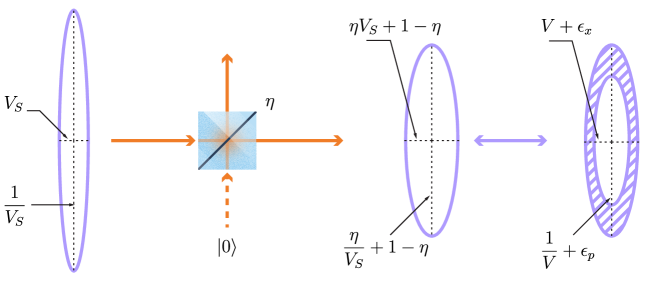
Figure 1: Evolution of a pure squeezed state with quadrature variances $V_{S},1/V_{S}$ after attenuation $\eta$. The vacuum noise is added in both quadratures, however without the knowledge of $V_{S}$ and $\eta$ the output state can be viewed as a pure state with respective variances $V,1/V$ and with excess noise $\epsilon_{x}$ and $\epsilon_{p}$ in respective quadratures. The attribution of this noise to either of the quadratures, once it is untrusted, has different effect on the performance of CV QKD protocols.

3 CV QKD protocol with AS excess noise

To investigate the role of AS noise in the squeezed-state CV-QKD, we consider the prepare-and-measure (P&M) squeezed-state protocol, as shown in Fig. 2, in which a trusted party (hereafter referred to as Alice) generates a squeezed signal state with squeezed quadrature variance V and AS quadrature variance $1/V+\Delta V$, $\Delta V$ being the excess AS noise. Alice then modulates the squeezed quadrature and AS quadrature (here and further with no loss of generality we assume the $x$-quadrature to be squeezed) according to Gaussian distributed random variables $x_{m}$ and $p_{m}$ with variances $V_{x}$ and $V_{p}$, respectively. Note that while the secret key is typically obtained from the measurements of the squeezed quadrature, we assume that both quadratures are modulated in the general case, particularly for estimating the channel parameters. The modulated squeezed state is sent to a remote trusted party (hereafter referred to as Bob) via a quantum channel characterized by transmittance $T$, and quadrature excess noise $\epsilon$ (which we, without loss of generality, quantify with respect to the channel input). Bob then performs a homodyne detection to measure either x- or p-quadrature of the quantum state he receives. Alternatively, Bob can measure both quadratures simultaneously with a generally unbalanced heterodyne detector (double homodyne) with the balancing $t_{het}$ as shown in Fig. 2b. After a sufficient number of transmitted pulses are measured, trusted parties perform error correction and privacy amplification on their data to obtain the secret key. The lower bound on the secret key, secure against collective attacks (directly extendable to security against general attacks in the asymptotic regime [13]) is given by:

$$K_{\infty}^{DR/RR}=\text{Max}\{0,\beta I_{AB}-\chi_{AE/BE}\}$$ (1)

for direct reconciliation (DR) and reverse reconciliation (RR) respectively, when either Alice or Bob is the reference side for the error correction of the key data. Here $\beta\in(0,1)$ stands for the post-processing (error-correction) efficiency, which scales down the achievable classical mutual information $I_{AB}$ between Alice and Bob, $\chi_{AE}$ and $\chi_{BE}$ are the upper bounds on the accessible information of an eavesdropper (hereafter referred to as Eve) on Alice’s or Bob’s data in DR and RR scenarios respectively, referred to as the Holevo bound [31]. Mutual information between Alice and Bob’s data sets $I_{AB}$ can be calculated from the variances and covariance of Alice and Bob’s data (with variances $V_{A}$ and $V_{B}$ respectively) and reads

$$I_{AB}=\frac{1}{2}\log_{2}\left[\frac{V_{A}}{V_{A|B}}\right]=\frac{1}{2}\log_{2}\left[\frac{V_{B}}{V_{B|A}}\right].$$ (2)

The conditional variance $V_{i|j}=V_{i}-C^{2}_{ij}/V_{j}$ (for $i=B,A$ and $j=A,B$ respectively) is obtained from the variances $V_{i,j}$ and covariance $C_{ij}$ of Alice and Bob data. The Holevo bounds are obtained from the von Neumann entropy of the state available to Eve $S(E)$ before and $S(E|A/B)$ after conditioning on the measurements by Alice or Bob for DR or RR respectively, $\chi_{AE/BE}=S(E)-S(E|A/B)$.
To assess the amount of information on the raw key available to Eve, we model this protocol using the general equivalent entanglement-based (EB) scheme presented in [18], as shown in Fig. 2b. This scheme involves coupling two oppositely squeezed states with $x$-quadrature variances $V_{1}$ and $V_{2}$ so that Alice then performs heterodyne detection on her mode A by coupling it on a balanced beamsplitter to a mode containing a pure squeezed state with $V_{m}$ $x$-quadrature variance.

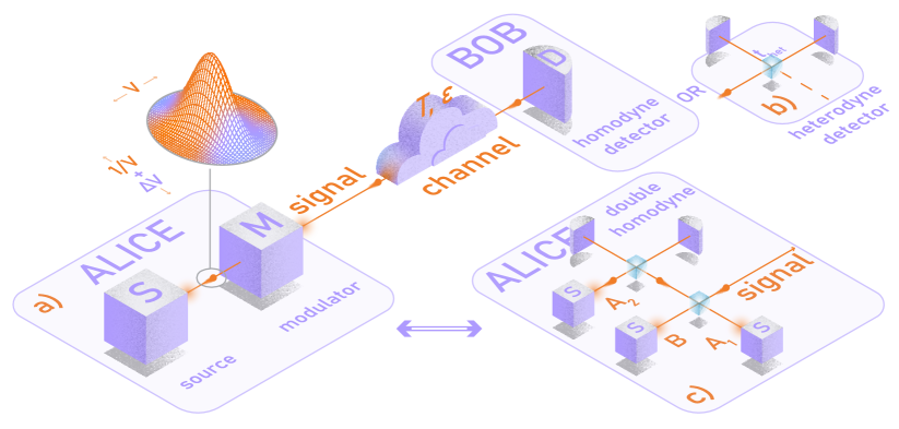
Figure 2: a) Prepare and measure scheme of a CV QKD protocol with noisy squeezed states. Alice modulates the squeezed state, characterized by the squeezed variance $V$ and AS excess noise $\Delta V$, according to normally distributed random variables and sends the Gaussian modulated squeezed state through a quantum channel characterized by transmittance $T$ and excess noise $\epsilon$. Bob at his end performs homodyne detection or b) unbalanced heterodyne detection with $t_{het}$. c) Equivalent general source model based on the balanced coupling of two oppositely squeezed states in modes $A_{1}$ and $B$ with different squeezed variances $V_{1}$, $V_{2}$ and a balanced heterodyne measurement at the Alice’s side, fed by a squeezed state with variance $V_{m}$ in mode $A_{2}$.

We analyze security of the protocol against Gaussian collective attacks, which were shown optimal against Gaussian CV QKD [32, 33], by obtaining the Holevo bound from the covariance matrices of the respective states shared between the trusted parties and an eavesdropper. The three-mode covariance matrix of the general EB scheme, taking into account the effect of the quantum channel in mode B, is

$$\gamma_{A_{1}A_{2}B}=\bNiceMatrix[margin]\gamma_{A_{1}}&\sigma_{A}\sqrt{T}\sigma_{AB}\\ \sigma_{A}\gamma_{A_{2}}\sqrt{T}\sigma_{AB}\\ \sqrt{T}\sigma_{AB}\sqrt{T}\sigma_{AB}\gamma_{B},$$ (3)

where the submatrices are

γ_A_1=γ_A_2=[V1+V2+2Vm400Vm(V1+V2)+2V1V24V1V2Vm], σ_A=[V1+V2-2Vm400Vm(V1+V2)-2V1V24V1V2Vm],

σ_AB=[V2-V12200V1-V222V1V2],  γ_B=[T(V1+V22+ϵ)+1-T00T(V1+V22V1V2+ϵ+ΔV_u)+1-T].

When Bob performs imbalanced heterodyne measurement, the covariance matrix $\gamma_{A_{1}A_{2}BB^{\prime}}$ reads

$$\bNiceMatrix[margin]\gamma_{A_{1}}&\sigma_{A}\sqrt{t_{het}T}\sigma_{AB}-\sqrt{(1-t_{het})T}\sigma_{AB}\\ \sigma_{A}\gamma_{A_{2}}\sqrt{t_{het}T}\sigma_{AB}-\sqrt{(1-t_{het})T}\sigma_{AB}\\ \sqrt{t_{het}T}\sigma_{AB}\sqrt{t_{het}T}\sigma_{AB}t_{het}\gamma_{B}+1-t_{het}\sqrt{1-t_{het}}\sqrt{t_{het}}(\mathds{1}-\gamma_{B})\\ -\sqrt{(1-t_{het})T}\sigma_{AB}-\sqrt{(1-t_{het})T}\sigma_{AB}\sqrt{1-t_{het}}\sqrt{t_{het}}(\mathds{1}-\gamma_{B})(1-t_{het})\gamma_{B}+t_{het}.$$ (4)

The squeezed variances of the prepare-and-measure and entanglement-based
schemes are related by the equivalence conditions [18]:

$$V_{1,2}=V+V_{x}\pm\sqrt{\frac{(V+V_{x})[V_{x}+VV_{p}(V+V_{x})]}{1+VV_{p}}},$$ (5)

$$V_{m}=\frac{V^{2}V_{p}(V+V_{x})}{V_{x}(1+VV_{p})}.$$ (6)

The trusted parties may assume the AS noise $\Delta V$ to be either trusted (hence, being out of control by an eavesdropper) or untrusted (fully controlled by Eve). We further denote the trusted and untrusted AS noise as $\Delta V_{t}$ and $\Delta V_{u}$, respectively. We model the trusted AS noise by redefining the modulation variance of the AS quadrature $V_{p}\rightarrow V_{p}+\Delta V_{t}$. On the other hand, the untrusted AS noise $\Delta V_{u}$ is added to the AS quadrature similarly to the channel noise $\epsilon$.

In the worst-case scenario, we assume that Eve can purify the state shared between Alice and Bob; thus $S(E)=S(AB)$, where $S(AB)$ is the Von Neumann entropy of the state shared between trusted parties, it can be calculated from the bosonic entropic function [34], as $S(AB)=\sum^{3}_{i=1}G[(\lambda_{i}-1)/2]$, where $\lambda_{1,2,3}$ are the symplectic eigenvalues of the covariance matrix $\gamma_{AB}$ and $G(x)=(x+1)\log(x+1)-x\log x$. Similarly, conditional entropies $S(E|A)$ and $S(E|B)$ can be obtained from the corresponding conditional covariance matrices:

$$\gamma_{i|j}=\gamma_{i}-\sigma_{ij}(X.\gamma_{j}.X)^{MP}\sigma^{T}_{ij},$$ (7)

where $i=A,B$ and $j=B,A$ respectively, with matrices $X=Diag(1,0)$ for x-quadrature measurement and $X=Diag(0,1)$ for p-quadrature measurement, while for the heterodyne measurement the conditioning (7) has to be applied twice on both x- and p-quadrature measurements on the two modes of the heterodyne detector.
Although for the two-mode conditional matrices, the symplectic eigenvalues can be found analytically, the eigenvalues of the 3-mode covariance matrix (3) and the larger matrices are found numerically to be used further in the calculation of the Holevo bound and the key rates.

The mutual information and the Holevo bound depend on the type of measurement Bob performs. We consider two major scenarios as follows:

Bob’s homodyne measurement approach:

Bob performs homodyne detection on mode $B$ and switches between the measurement of squeezed and AS quadratures with a certain ratio. Equivalently, Alice can choose different quadratures (x or p) to be squeezed to achieve the same result. Since Bob measures both the quadratures, albeit at different times, when all the measurements are utilized for key generation, the asymptotic key rate $K_{\infty}$ from Eq. (1) is given by

$$K_{\infty}=\underbrace{\text{Max}\{0,I^{x}_{AB}-[S(AB)-S(A|B^{x})]\}}_{K^{x}_{\infty}}+\underbrace{\text{Max}\{0,I^{p}_{AB}-[S(AB)-S(A|B^{p})]\}}_{K^{p}_{\infty}}$$ (8)

For simplicity, we present all the key rate expressions hereafter in the more relevant RR scenario (allowing for much longer secure distances [8]). The key rate expressions for DR can be obtained by interchanging modes $A$ and $B$. $K^{x}_{\infty}$ and $K^{p}_{\infty}$ are the asymptotic key rates between Alice and Bob, when Bob performs homodyne measurement of squeezed and AS quadrature, respectively. $I^{i}_{AB}$ and $S(AB)-S(A|B^{i})$ are the mutual information and Holevo bound when Bob performs the homodyne measurement of squeezed ($i=x$) and AS quadrature ($i=p$).

Bob’s heterodyne measurement approach:

Bob performs imbalanced heterodyne measurement, as shown in Fig. 2b. Similarly to the previous case, the asymptotic key rate expression is different depending on whether the AS quadrature measurements are used for key generation. The asymptotic key rate when AS quadrature is used for key generation is (where $B^{x}$ and $B^{p}$ means that Bob measures x-quadrature in mode B and p-quadrature in mode $B^{\prime}$ of the heterodyne detector):

$$K_{\infty}=\text{Max}\{0,I^{x}_{AB}+I^{p}_{AB}-\left[S(AB)-S(A|B^{x}B^{p})\right]\}$$ (9)

When the AS quadrature is not used for key generation, the asymptotic key rate is:

$$K_{\infty}=\text{Max}\{0,I^{x}_{AB}-\left[S(AB^{x}B^{p})-S(AB^{p}|B^{x})\right]\}$$ (10)

Since the trusted parties do not use the AS quadrature for key generation, they can also disclose (publicly announce) the AS quadrature measurement outcomes, which can provide a practical advantage in parameter estimation and choosing error correction codes. The key rate when AS quadrature measurements are disclosed is:

$$K_{\infty}=\text{Max}\{0,I^{x}_{AB}-\left[S(AB^{x}|B^{p})-S(A|B^{x}B^{p})\right]\}$$ (11)

To study the optimal performance of CV QKD with untrusted AS noise (on top of symmetric noise $\epsilon$) in the asymptotic regime, we only consider the measurement of squeezed quadrature by Bob.

4 Performance of CV QKD with noisy squeezed states

4.1 Asymptotic key rate

For the case when the AS noise can be trusted and the channel is purely attenuating ($\epsilon=0$), there is no need to build an equivalent EPR state, as the information available to Eve can be obtained directly from the other output of the beamsplitter, which explicitly models the channel attenuation [35]. The covariance matrix of the state available to Eve is

$$\gamma_{E}=\left[\begin{array}[]{cc}(1-T)(V_{x}+V)+T&0\\ 0&(1-T)(\frac{1}{V}+\Delta V_{t})+T\end{array}\right],$$ (12)

where $\Delta V_{t}$ is the trusted AS excess noise. Conditional state of Eve on the homodyne measurement of $x$-quadrature by Bob (the most basic scenario, as the AS quadrature measurements are not required in the asymptotic regime) is

$$\gamma_{E|B}=\left[\begin{array}[]{cc}(V+V_{x})/[1+T(-1+V+V_{x})]&0\\ 0&T+(1-T)(1/V+\Delta V_{t})\end{array}\right].$$ (13)

Conditional state of Eve on measurement of $x$-quadrature by Alice is

$$\gamma_{E|A}=\left[\begin{array}[]{cc}(1-T)V+T&0\\ 0&T+(1-T)(1/V+\Delta V_{t})\end{array}\right].$$ (14)

The symplectic eigenvalues of the single mode matrices $\gamma_{y}$ given above (where $y$ is $E,E|A$ and $E|B$) are obtained by the relation $\lambda_{y}=\sqrt{Det(\gamma_{y})}$. Mutual information between trusted parties is not influenced by AS noise, as the AS quadrature is not used for key generation. On the other hand it reduces the Holevo bound and we obtain the following analytical expressions for the Holevo bound in the limit of infinitely strong AS noise:

$$\lim_{\Delta V_{t}\to\infty}\chi_{EB}=\frac{1}{2}\log_{2}\left[\frac{[V+V_{x}-T(V+V_{x}-1)][1+T(V+V_{x}-1)]}{V+V_{x}}\right]=I_{EB}$$ (15)

$$\lim_{\Delta V_{t}\to\infty}\chi_{EA}=\frac{1}{2}\log_{2}\left[1+\frac{V_{x}(1-T)}{T+V(1-T)}\right]=I_{EA},$$ (16)

where $I_{EB}$ and $I_{EA}$ are the classical mutual information quantities between Eve and Bob, and Eve and Alice respectively. This implies that for a purely lossy channel and infinite trusted AS noise, collective attacks are equivalent to individual attacks. Since $\lim_{\Delta V_{t}\to\infty}\chi_{EB}$ is a function of $(V+V_{x})$, where $0<V\leq 1$, for large modulation variance $V_{x}$, the Holevo bound for RR barely depends on the degree of squeezing. In the limit of infinitely strong signal modulation $V_{x}\to\infty$ and infinitely strong signal squeezing $V\to 0$ the improvement to the Holevo bound due to the strong trusted AS noise vanishes and the key rate analytically hits the known bounds for the squeezed-state protocol, $\log_{2}\left[T/(1-T)\right]$ for DR and $\log_{2}\left[1/(1-T)\right]$ for RR [36].

In the presence of channel noise, no simple analytical expressions can be obtained for the Holevo bound, as we rely on the 3-mode purification described in Sec.3. The presence of trusted noise can improve tolerance to untrusted channel noise, as can be seen from the plots in Fig. 3, where we model the performance of the protocol assuming realistic error correction efficiency of $\beta=0.95$ [37] and optimizing the modulation variance. The improvement by the trusted AS noise is more evident in DR than in RR, being a case of the ”fighting noise with noise” method [16, 36]. Interestingly, a moderately squeezed source ($V=0.5$ SNU) in the presence of optimal trusted AS noise has a higher tolerance to channel noise than the protocol with a higher degree of pure signal squeezing of the source state. On the other hand, when the AS noise cannot be trusted, the tolerance of the protocol to channel noise is significantly reduced, as can be seen from the plots in Fig. 4, as the presence of untrusted AS noise increases the Holevo bound. This emphasises the need to control and to estimate noise in the AS quadrature, which would otherwise lead to underestimation of the Holevo bound.

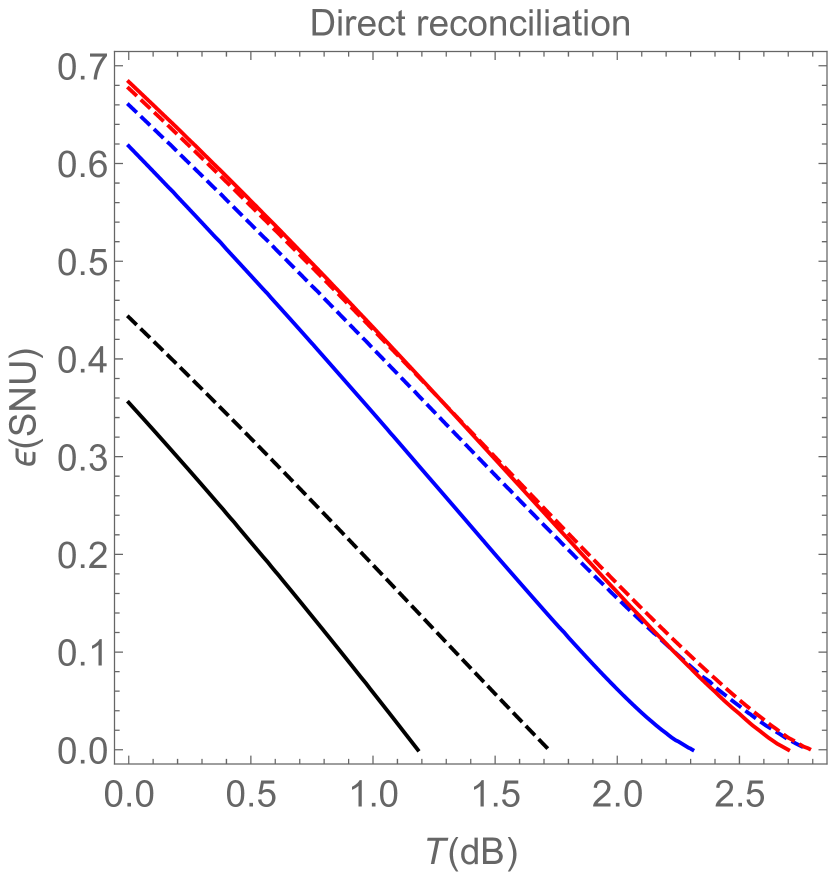
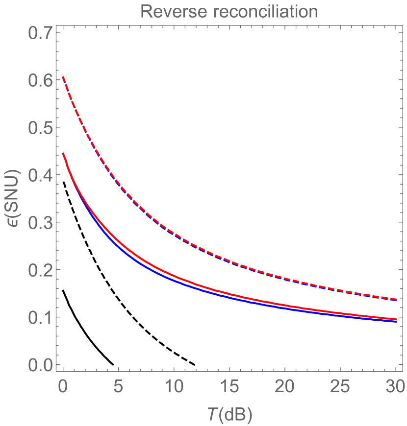
Figure 3: Maximal tolerable channel noise ($\epsilon$) with respect to channel attenuation $T$ (in dB scale) for highly squeezed $V=0.1$ SNU (dashed) and moderately squeezed $V=0.5$ (solid) source state with optimised modulation variance and reconciliation efficiency $\beta=0.95$, in the presence of 0.5 SNU AS noise, when it is trusted (blue) and when it is untrusted (black). The red plot shows the tolerance to channel noise when 10 SNU trusted AS noise is added. Adding trusted AS noise showed no difference in the tolerance for RR when the source state is highly squeezed (0.1 SNU), hence the blue dashed plot and the red dashed plot overlap, while adding trusted AS noise drastically improved the tolerance in DR when the source state is moderately squeezed.

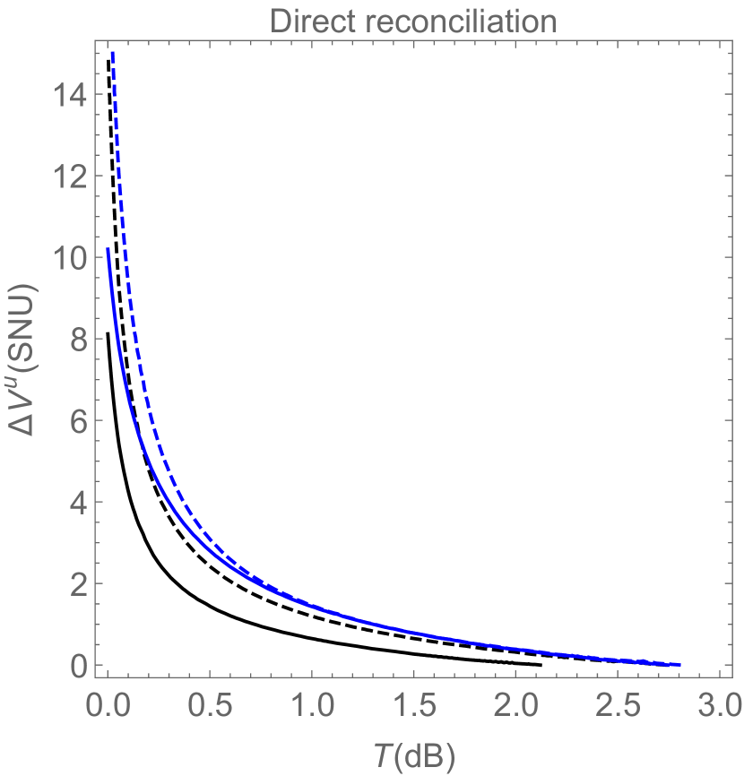
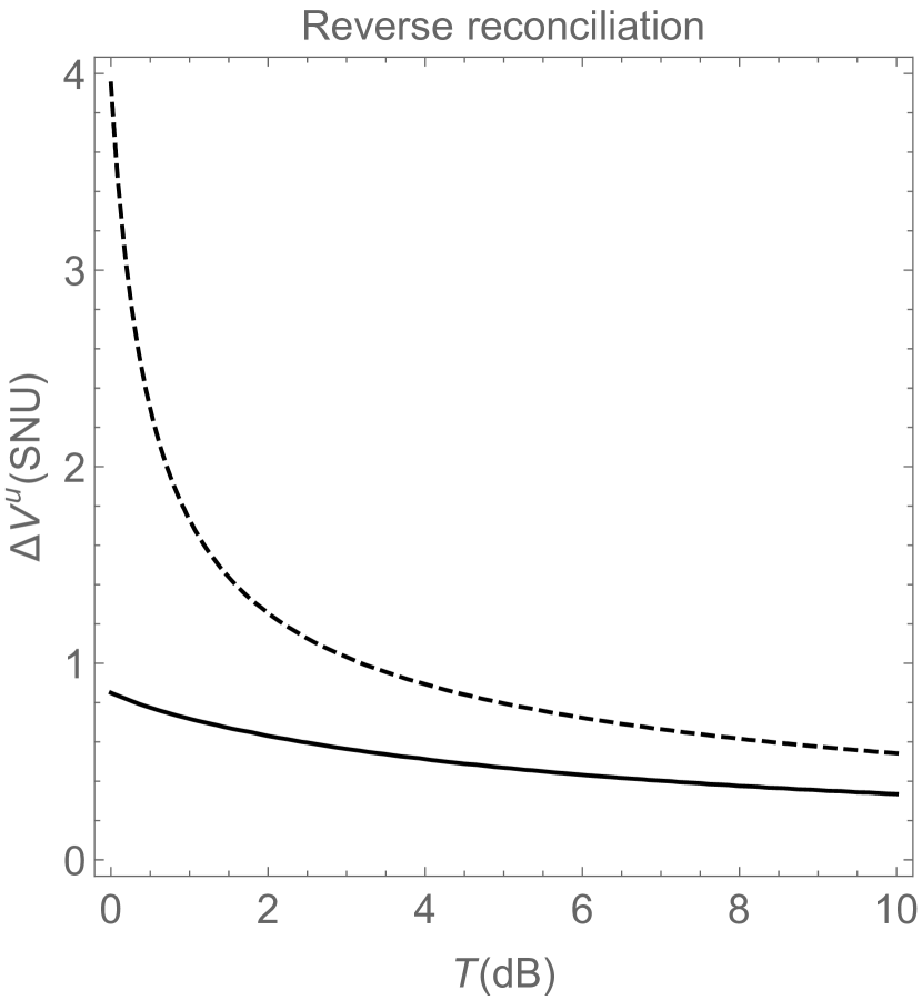
Figure 4: Tolerable untrusted AS noise ($\Delta V_{u}$) with respect to channel attenuation $T$, for highly squeezed ($V=0.1$ SNU, dashed) and moderately squeezed ($V=0.5$ SNU, solid) states, with optimized modulation variance ($\text{Max}[V_{x}]=10$ SNU). Shown with (blue) and without (black) trusted AS noise ($\Delta V_{t}=10$ SNU). Negligible impact of trusted noise in RR. Channel noise: $\epsilon=0.01$ SNU, reconciliation efficiency: $\beta=0.95$.

4.2 Finite-size key rate

A necessary requirement to verify the security of QKD is to estimate the channel parameters from which the Holevo bound can be found. Channel parameters can only be estimated within a certain confidence interval, which is inversely propositional to the number of states sent to Bob. Typically part of the received data is used for parameter estimation, and the rest is used for the key generation [38]. It has been also shown that all the measurements can be used for both parameter estimation and key generation by performing error correction before parameter estimation [39]. For completeness, we consider both cases, when part of the measurements are disclosed for parameter estimation (see B), and when all the measurements are used for parameter estimation and key generation.

As established in the previous section, AS noise is detrimental to the security of the squeezed-state protocol when it is untrusted. The adverse effect of AS noise is further amplified in the practical finite-size regime of limited data ensembles, as the presence of AS noise requires one to make the estimation of the channel noise independently for both the quadratures, utilising more available resources for parameter estimation, unless all the measurement outcomes are used both for the key and for the estimation.

In order not to underestimate the information available to the eavesdropper, we use the lower bound for the confidence interval of channel transmittance $T^{low}$ and the upper bound for channel noise $V_{\epsilon}^{up}$. We consider $\mathbf{E}(T^{low})=T-6.5\Upsilon$ and $\mathbf{E}(V_{\epsilon}^{up})=V_{\epsilon}+6.5s$ corresponding to the estimation error probability of $10^{-10}$, $\sigma$ and $s$ are the standard deviations of the channel transmittance and noise, respectively. In order to effectively use the available resources, we extend the parameter estimation from [12, 38] to use the measurements of both quadratures to potentially make a better estimation of the channel parameters (refer to B for details). We obtain the following finite-size key rate:

$$K_{finite}=\frac{n_{k}}{N}[K_{\infty}(T^{low},\hat{V}_{\epsilon_{x}}^{up},\hat{V}_{\epsilon_{p}}^{up})-\Delta(n)]$$ (17)

In this context, $\Delta(n)$ denotes the correction term for privacy amplification[12]. When all the measurements are used for key generation and parameter estimation, the finite-size key rate becomes:

$$K_{finite}=K_{\infty}(T^{low},\hat{V}_{\epsilon_{x}}^{up},\hat{V}_{\epsilon_{p}}^{up})-\Delta(N)$$ (18)

As using AS quadrature for the parameter estimation is detrimental to achieving large distances, the optimal finite-size key rate for the homodyne measurement approach is given by (17), with $n_{k}=m$ ($m$ is the number of measurements of the squeezed quadrature).

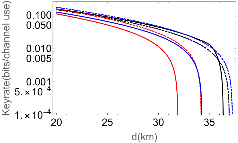
(a) $\Delta V_{t}=0$, $\Delta V_{u}=0$, $N=10^{6}$

(b) $\Delta V_{t}=0$, $\Delta V_{u}=0$, $N=10^{7}$

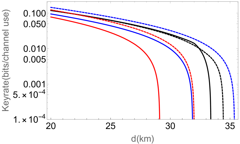
(c) $\Delta V_{t}=0$, $\Delta V_{u}=0.05$, $N=10^{6}$

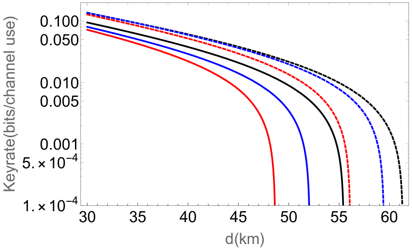
(d) $\Delta V_{t}=0$, $\Delta V_{u}=0.05$, $N=10^{7}$

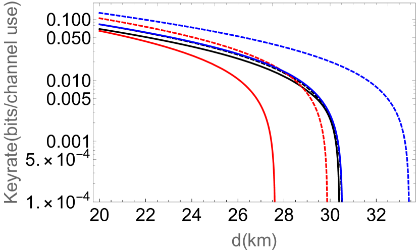
(e) $\Delta V_{t}=5$, $\Delta V_{u}=0$, $N=10^{6}$

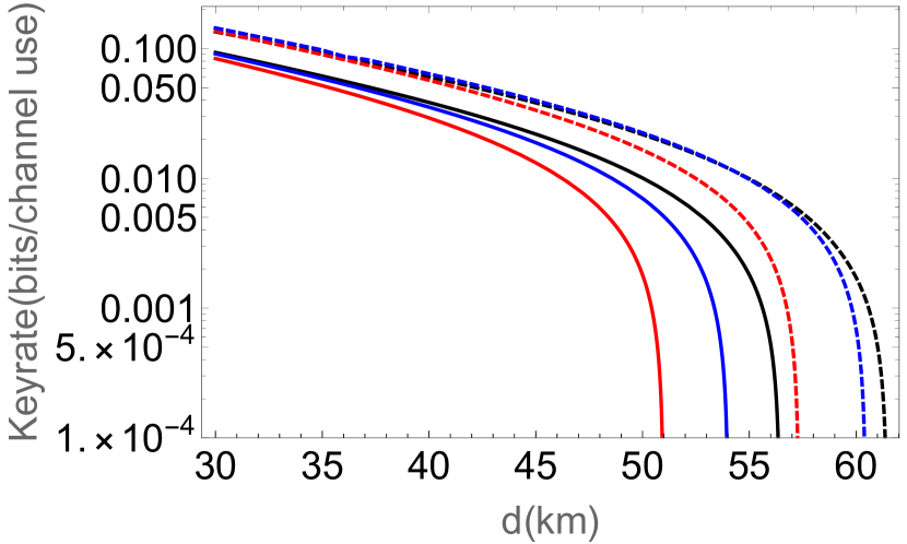
(f) $\Delta V_{t}=5$, $\Delta V_{u}=0$, $N=10^{7}$

Figure 5: Finite-size key rate vs. distance when Bob performs biased homodyne detection (black), imbalanced heterodyne detection (blue) and when Bob performs imbalanced heterodyne detection and discloses AS measurement results (red), all in the RR scenario. The dashed plot represents a highly squeezed source state ($V=0.1$ SNU) and the solid plot represents a moderately squeezed source state ($V=0.5$ SNU). Modulation variances $V_{x}$ and $V_{p}$, transmittance of beamsplitter for heterodyne detection $t_{het}$, ratios of available resources used for key generation $r_{k}$, and parameter estimation $r_{x}$ and $r_{p}$ are optimized. The reconciliation efficiency is $\beta=0.95$, the channel noise is $\epsilon=0.05$ SNU, and the channel attenuation is 0.2 dB/km.

In Fig. 5, our analysis reveals distinct trends based on the degree of squeezing in the source state. Imbalanced heterodyne measurements demonstrate superior performance with small block sizes ($N=10^{6}$) for highly squeezed states (dashed plots), while biased homodyne detection becomes more favorable with larger block sizes ($N=10^{7}$), see Fig. 55(b), 5(d) and 5(f). Notably, biased homodyne measurements consistently outperform other strategies for moderately squeezed states. In scenarios marked by elevated trusted noise and reduced block lengths (Fig. 55(e)), imbalanced heterodyne measurement proves significantly more efficacious than biased homodyne measurement. Furthermore, we present key rates when the AS quadrature measurement in imbalanced heterodyne measurements is disclosed publicly (red plots in Fig. 5 and 6), showcasing its potential contributions to parameter estimation and the selection of optimal error correction codes.
Fig. 6 adds complexity to the narrative, revealing that the efficacy of imbalanced heterodyne measurements is contingent on the presence of channel noise. Specifically, imbalanced heterodyne measurement emerges as consistently superior in scenarios characterized by a substantial amount of channel noise ($\epsilon>0.1$ SNU), while biased homodyne measurement excels in low-channel-noise conditions ($\epsilon<0.1$ SNU). The interplay of measurement strategies with channel noise highlights the nuanced considerations necessary for optimizing squeezed-state CV quantum communication systems.

Turning our attention to untrusted AS noise (Fig. 7), we observe a lack of significant differences in tolerance between biased homodyne and imbalanced heterodyne measurements for RR. For DR, the biased homodyne measurement strategy is always superior. The absence of a one-size-fits-all solution requires careful analysis to select the optimal measurement strategy in specific experimental conditions.

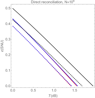
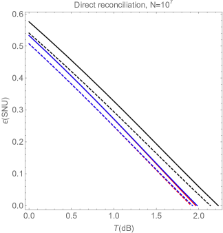
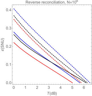
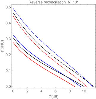
Figure 6: Tolerance to channel noise for biased homodyne (black) and imbalanced heterodyne measurement by Bob, when AS quadrature measurement is publicly announced (red) and when it is not announced (blue) in different reconciliation scenarios and at different data block sizes. The modulation variance of the squeezed and AS quadrature $V_{x}$ and $V_{p}$, ratio of squeezed quadrature measurement for biased homodyne detection and the beamsplitter transmittance $t_{het}$ of imbalanced heterodyne measurement are optimised (see Fig. 12 for optimum ratio and transmittance). Reconciliation efficiency $\beta=0.95$ and the untrusted AS noise $\Delta V_{u}=0.2$ SNU.

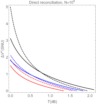
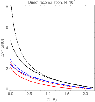
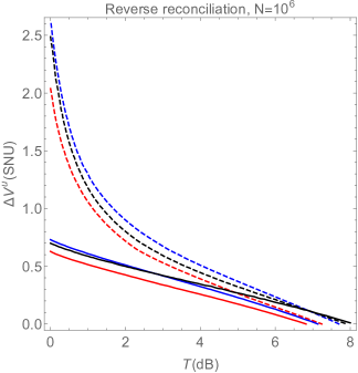
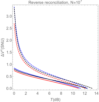
Figure 7: Tolerance to untrusted AS noise $\Delta V_{u}$ for biased homodyne (black) and imbalanced heterodyne measurement by Bob, when AS quadrature measurement is publicly announced (red) and when it is not announced (blue) in different reconciliation scenarios and at different data block sizes. The modulation variance of the squeezed and AS quadrature $V_{x}$ and $V_{p}$, ratio of squeezed quadrature measurement for biased homodyne detection and the beamsplitter transmittance $t_{het}$ of imbalanced heterodyne measurement are optimised. Reconciliation efficiency $\beta=0.95$ and the channel noise $\epsilon=0.01$ SNU.

5 Anti-squeezing noise in fluctuating channels

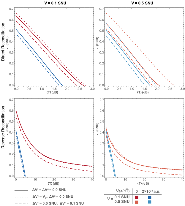
Figure 8: Maximal tolerable excess noise ($\epsilon$ in SNU) at the input of the channel with respect to mean channel attenuation $\langle T\rangle$ (in dB scale) for highly squeezed $V=0.1$ SNU (left column) and moderately squeezed $V=0.5$ SNU (right column) source state, in the absence of AS noise (solid), with trusted AS noise $\Delta V_{t}=V_{x}$ (short dash), and untrusted AS noise $\Delta V_{u}=0.1$ SNU (long dash). Red lines correspond to the absence of transmittance fluctuations $Var(\sqrt{T})=0$, and blue to $Var(\sqrt{T})=2\times 10^{-2}$. Modulation variance $V_{x}$ is optimized for reconciliation efficiency of $\beta=95\%$, AS noise and respective fading.

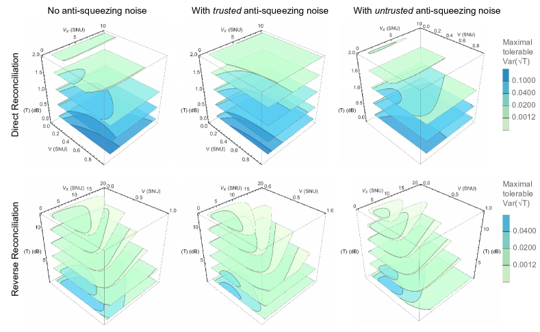
Figure 9: Maximal tolerable level of transmittance fluctuations $Var(\sqrt{T})$ against squeezing $V$, in DR (top row) and RR (bottom row) without AS noise (left column), with trusted AS noise $\Delta V_{t}=V_{x}$ (middle column), and untrusted AS $\Delta V_{u}=0.1$ SNU (right column). Channel excess noise $\epsilon=0.1$ SNU, and reconciliation efficiency $\beta=95\%$

While in the previous sections we assumed the channel transmittance to be stable, which typically corresponds to fiber-type channels, in the free-space realizations it is usually not the case and the atmospheric channel transmittance fluctuates due to the turbulence effects, we further refer to such transmittance fluctuations as to the channel fading. Although the changes of transmittance are slower than the clock rate of the protocol, such attenuation fluctuations during data accumulation can significantly impede achievable secure key rate [20, 21]. The overall state shared between trusted parties after the fading channel is generally non-Gaussian and is described by the Wigner function, which is the weighed convex sum of Wigner functions that characterize shared state when Bob’s subsystem was transmitted through a channel with fixed transmittance $T_{i}$ that occurs with probability $\tau_{i}$, with $\sum^{M}_{i=1}\tau_{i}=1$ [40]. While the first moments remain zero, the second moments $\gamma_{AB}$ of the resulting state are hence the convex combination with transmittance $T_{i}$ and transmittance coefficient $\sqrt{T_{i}}$ of all $i\in[1,M]$. Extremality of Gaussian states [41] and subsequent optimality of Gaussian collective attacks [32, 33] allows us to gaussify the overall mixed state, i.e. base further security analysis on the covariance matrix $\gamma_{AB}$, which is now evidently a function of $\langle T\rangle$ and $\langle\sqrt{T}\rangle$, without underestimating the eavesdropper. In the current section we consider the homodyne-based protocol as the best performing in the asymptotic regime, and allowing to reach longer distances in finite-size regime. Bob’s subsystem after the fading channel is described by

$$\gamma_{B}=\left[\begin{array}[]{cc}\langle T\rangle(V+V_{x}-1)+1&0\\ 0&\langle T\rangle(1/V+V_{p}+\Delta V-1)+1\end{array}\right],$$ (19)

and correlated to Alice’s mode as:

$$\varsigma_{AB}=\left[\begin{array}[]{cc}\langle\sqrt{T}\rangle\frac{V_{2}-V_{1}}{2\sqrt{2}}&0\\ 0&\langle\sqrt{T}\rangle\frac{\frac{1}{V_{2}}-\frac{1}{V_{1}}}{2\sqrt{2}}\end{array}\right]$$ (20)

The mutual information (in $x$-quadrature) without AS noise $\Delta V$ is therefore:

$$I_{AB}=\frac{1}{2}\log_{2}\left[\frac{1+\langle T\rangle(V+\epsilon-1+V_{x})}{1-\langle\sqrt{T}\rangle^{2}V_{x}+\langle T\rangle(V+\epsilon-1+V_{x})}\right].$$ (21)

A fading channel can be equivalently represented as a channel with fixed transmittance $\langle\sqrt{T}\rangle^{2}$ and fading-related variance-dependent excess noise $\varepsilon_{x}^{f}=Var(\sqrt{T})(V+V_{x}-1)$ and $\varepsilon_{p}^{f}=Var(\sqrt{T})(1/V+V_{p}+\Delta V-1)$ in $x$- and $p$-quadratures respectively, contrary to symmetrical fading-related noise in the coherent-state protocol [20]. The noise related to fading is to be assumed untrusted, as the transmittance fluctuations can be fully controlled by Eve. This represents another strongly negative impact of AS noise in the fluctuating channels, even if the noisy source is initially trusted. Such noise necessitates the characterization of transmittance coefficient variance $Var(\sqrt{T})=\langle T\rangle-\langle\sqrt{T}\rangle^{2}$ and consequent adaptation of modulation $V_{x(p)}$ and squeezing variance $V$ for optimal secure key rate. For weak atmospheric turbulence one can expect $Var(\sqrt{T})\leq 0.01$, and $Var(\sqrt{T})>0.04$ for strong turbulence [21]. Mutual information (21) reduces to (2) when fluctuations of transmittance are negligible, i.e. $M=1$ and $\tau_{i=1}=1$ or $Var(\sqrt{T})=0$. The upper bound on Eve’s accessible information $\chi_{AE}$ or $\chi_{BE}$ is evaluated based on $\gamma_{AB}(\langle T\rangle,Var(\sqrt{T}))$ as well. For further details regarding the modelling and security analysis of atmospheric channels in CV QKD see [20].

The effect of transmittance fluctuations and AS noise on the security of the squeezed-state CV QKD protocol is shown in Fig. 8. The value of transmittance coefficient variance is set to $Var(\sqrt{T})=0.02$ which corresponds to weak-to-moderate turbulence regime [42], where beam shape deformation, broadening and wandering are expected, corresponding to daytime operation of a short free-space atmospheric link.

Regardless of the choice of reconciliation side, level of squeezing in the signal quadrature, and assumptions on the AS noise, transmittance fluctuations have a detrimental effect on the tolerance to excess noise $\epsilon$ and loss $\langle T\rangle$ of the CV QKD protocol. In the absence of fading, the protocol performances are slightly improved by trusted AS noise presence (with a negligible effect in some regimes for strong AS and RR), while untrusted AS noise leads to performance degradation. In the presence of already weak fading, the positive effect of strong trusted AS recedes and it can be helpful for DR protocols using moderately squeezed signal states. For RR protocol, however, AS is generally limiting the range of secure parameters. The sensitivity of the protocol established over fading channels underlines the need for characterization and optimization of the transmitter, as shown in Fig. 9. We show the maximal tolerable fading dependence on the level of squeezing $V$ and modulation variance $V_{x}$ at different values of mean channel loss $\langle T\rangle$. Trusting AS enables a significantly wider range of tolerable atmospheric conditions when DR protocol is used, and allows for more flexible choice of optimal combination of squeezing and modulation variance. Untrusted AS, as expected, necessitates for squeezing to be optimized (preferably to high values) and limits $V_{x}$ to few SNU. With RR protocol the range of optimal squeezing $V$ steers towards lower values. Therefore, even if trusted, proper characterization, control of AS noise and consequent parameter optimization is crucial for implementations in fading (particularly free-space) channels.

6 Conclusion

In this work, we perform an exhaustive investigation into the role of the noise in squeezed signal states in CV QKD, considering collective attacks in the asymptotic as well as finite-size regimes, and incorporating free-space channel fading. We show how the noise in the signal squeezing can unavoidably appear as the result of optical losses already in the state generation. The impact of this noise however greatly depends on whether it can be assumed trusted, i.e., originating from the trusted source and not controlled by an eavesdropper, or not. In the case, when this noise is trusted, we firmly assume that it is contained in the AS quadrature. Such trusted noise can even slightly reduce the Holevo bound, leading to analytical convergence to individual attacks in the limit of strong noise. The trusted AS noise can also be helpful in DR scenario as a counter-measure against the channel noise. In the finite-size regime, however, already the trusted AS noise can limit the efficiency of parameter estimation and requires optimization of the protocol and the estimation strategies. Considering biased homodyne detection and unbalanced heterodyne detection as the possible strategies on the receiver side and taking into account the possibility to announce the outcomes of the AS quadrature measurements, we identify the optimal protocol implementations. Our findings show that biased alternation between homodyne measurements of squeezed and AS quadrature of signal field, followed by disclosure of the latter, allows to extend the secure distance. However, simultaneous measurement of both quadratures can still be advantageous in certain regimes, especially for shorter data accumulation times, resulting in shorter data block sizes. Finally, we consider the fading channels with fluctuating transmittance, which is typical for free-space atmospheric channels, and show that even trusted AS noise transforms to the untrusted AS noise due to fading. This emphasizes the importance of the state purity for squeezed-state CV QKD realizations in free-space channels already with the trusted sources. Our findings present the methods for protocol optimizations, including measurement and estimation techniques, as well as suggest the experimental efforts towards the signal state purity for efficient squeezed-state CV QKD. The obtained results pave the way towards practical and efficient realization of the squeezed-state QKD, they can be directly applied in point-to-point protocols as well as in QKD-based communication networks, where great diversity of implementation conditions and combination of various protocols and link types is anticipated.

Appendix A Squeezed-state noise allocation

In our CV QKD analysis we made a deliberate choice by incorporating all the noise, that transformed our initially pure squeezed state into a noisy one, within the AS quadrature. One might contend that the noise could equally be distributed across the squeezed quadrature. This decision holds no consequences when the noise is trusted and does not augment Eve’s knowledge of the shared state between the trusted parties. However, in cases when the noise, responsible for impurities in the pure squeezed state, cannot be trusted, we are compelled to consider the most pessimistic option. This implies assigning all the noise to the AS quadrature, a demonstration of which is presented in this section.

To evaluate the potential information leakage arising from an impure squeezed state, let’s consider a scenario where the exclusive source of information available to Eve is the impure squeezed state, characterized by a squeezed quadrature variance $\tilde{V}_{s}=V+\epsilon_{x}<1$ and an AS quadrature variance $\tilde{V}_{as}=1/V+\epsilon_{p}>1/\tilde{V}_{s}$. The noise is distributed arbitrarily along the squeezed and AS quadratures, where $0<\epsilon_{x}<\tilde{V}_{s}-1/\tilde{V}_{as}$ and $\epsilon_{p}=\tilde{V}_{as}-1/(\tilde{V}_{s}-\epsilon_{x})$.

In an equivalent entanglement-based protocol for a P&M scheme, where Alice modulates the squeezed quadrature with a Gaussian distribution having modulation variance $V_{x}$, the protocol involves two squeezed states with x quadrature variances $V_{1}=V+V_{x}-\sqrt{(V+V_{x})V_{x}}$ and $V_{2}=V+V_{x}+\sqrt{(V+V_{x})V_{x}}$. These states are operated on a balanced beamsplitter, resulting in the following covariance matrix:

$$\gamma_{AB}=\left[\begin{array}[]{cccc}\frac{V_{1}+V_{2}}{2}&0&\frac{V_{2}-V_{1}}{2}&0\\ 0&\frac{1}{2}\left(\frac{1}{V_{2}}+\frac{1}{V_{1}}\right)&0&\frac{1}{2}\left(\frac{1}{V_{2}}-\frac{1}{V_{1}}\right)\\ \frac{V_{2}-V_{1}}{2}&0&\frac{V_{1}+V_{2}}{2}+\epsilon_{x}&0\\ 0&\frac{1}{2}\left(\frac{1}{V_{2}}-\frac{1}{V_{1}}\right)&0&\frac{1}{2}\left(\frac{1}{V_{2}}+\frac{1}{V_{1}}\right)+\epsilon_{p}\end{array}\right]$$ (22)

The conditional covariance matrix of Alice upon Bob’s squeezed quadrature measurement is $\gamma_{A|B}=Diag[(2V_{1}V_{2}+\epsilon_{x}(V_{1}+V_{2}))/(2\epsilon_{x}+V_{1}+V_{2}),(V_{1}+V_{2})/(2V_{1}V_{2})]$ and conditional covariance matrix of Bob upon Alice’s squeezed quadrature measurement is $\gamma_{B|A}=Diag[(2V_{1}V_{2})/(V_{1}+V_{2})+\epsilon_{x},1/2(1/V_{1}+1/V_{2})+\epsilon_{p}]$. The Holevo bound, which provides the upper bound on Eve’s knowledge of Alice’s or Bob’s measurement outcome, for DR or RR protocols, respectively, is obtained from the symplectic eigenvalues of the covariance matrices $\gamma_{AB}$, $\gamma_{A|B}$ and $\gamma_{B|A}$, as explained in Sec.3. Although the symplectic eigenvalues of $\gamma_{A|B}$ and $\gamma_{B|A}$ are easy to calculate (they are $\pm\sqrt{Det[\gamma_{A|B}]}$ and $\pm\sqrt{Det[\gamma_{B|A}]}$ respectively), the symplectic eigenvalues of $\gamma_{AB}$ do not have a simple form in general. However, we are able to obtain a simple symplectic eigenvalue expression for extreme cases, i.e., $\epsilon^{max}_{x}=\tilde{V}_{s}-1/\tilde{V}_{as}$ and $\epsilon_{p}=0$ or $\epsilon_{x}=0$ and $\epsilon^{max}_{p}=\tilde{V}_{as}-1/\tilde{V}_{s}$. When all the noise is considered to be in the squeezed quadrature, the symplectic eigenvalues of $\gamma_{AB}$ after using the P&M equivalence relations are $\{\pm 1,\pm(\sqrt{[\epsilon^{max}_{x}+V]/V}-1)/2\}$. When the noise is considered in AS quadrature the symplectic eigen values are $\{\pm 1,\pm(\sqrt{1+\epsilon^{max}_{p}[V+V_{x}]}-1)/2\}$. The Holevo bounds are: χ_RR(V,V_x,ϵ^max_x,0) &= G([ϵmaxx+V]/V-12)
 - G([(ϵmaxx+ V) (V + Vx)]/[V (ϵmaxx+ V + Vx)]-12)
χ_RR(V,V_x,0,ϵ^max_p) = G(1 + ϵmaxp(V + Vx)-12)
χ_DR(V,V_x,ϵ^max_x,0) = 0
χ_DR(V,V_x,0,ϵ^max_p) = G(1 + ϵmaxp(V + Vx)-12)
 - G(1 + ϵmaxpV-12) As $V>0$, $V_{x}>0$, and $\epsilon^{max}_{p}>\epsilon^{max}_{x}$ (where $\epsilon^{max}_{p}=(\tilde{V}{as}/\tilde{V}_{s})\epsilon^{max}_{x}$), the comparison of terms involving $G$ between $\chi_{RR}(V,V_{x},\epsilon^{max}_{x},0)$ and $\chi_{RR}(V,V_{x},0,\epsilon^{max}_{p})$, the larger arguments in the latter case result in greater values due to the monotonic nature of $G$. Additionally, it is worth noting that when all the noise is in the squeezed quadrature, $S(AB)=S(B|A)$, and when all the noise is in the AS quadrature, $S(A|B)=0$.
To gain insights into the impact of arbitrary noise distributions, we perform numerical investigations focusing on impure squeezed state obtained due to attenuation of pure squeezed state Fig. 1. Fig. 10 displays the Holevo bound versus excess squeezed quadrature variance $\epsilon_{x}$ for various transmittance values and degrees of squeezing, with the excess noise in the (AS) quadrature being $\epsilon_{p}=1+\eta(1/V_{s}-1)-1/(1+\eta[V_{s}-1]-\epsilon_{x})$. The plots provide intriguing insights into the consequences of employing an impure squeezed state. One notable observation is that, under worst-case considerations, increased impurity does not necessarily translate to reduced security. This phenomenon stems from the fact that a higher impurity in a noisy squeezed state does not inherently result in higher AS noise. To illustrate, consider the attenuation of a highly squeezed state ($V_{s}$ = 0.1 SNU) with beamsplitter transmittance values $\eta$ = 0.5 and $\eta$ = 0.7. Despite the state with higher losses being less pure, the maximum AS excess noise for $\eta$ = 0.5 is less than that for $\eta$ = 0.7.

In the context of DR, accounting for all the noise in the AS quadrature may not necessarily lead to a worse outcome. To delve deeper into this, we assess the key rate given by the equation:

$$K_{dr}=\frac{1}{2}\log_{2}\left(1+\frac{V_{x}}{\tilde{V}_{s}}\right)-\chi_{DR}(V,V_{x},\epsilon_{x},\epsilon_{p})$$ (23)

This evaluation is performed for noisy squeezed states with AS quadrature variance $\tilde{V}_{\text{as}}=10$ (black plot from Fig. 11) and $\tilde{V}_{\text{AS}}=5$ (blue plot from Fig. 11), considering squeezed quadrature variances $0.1\leq\tilde{V}_{s}\leq\tilde{V}_{s}^{\text{max}}$ and $0.2\leq\tilde{V}_{s}\leq\tilde{V}_{s}^{\text{max}}$, respectively. Here, $\tilde{V}_{s}^{\text{max}}$ represents the maximum $\tilde{V}_{s}$ for which a positive key rate can be achieved.

Fig. 11(a) illustrates the squeezed quadrature noise $\epsilon_{x}$ for which the key rate is minimized, considering the rest of the noise in the AS quadrature $\epsilon_{p}$. From the figure, we infer that for lower noise levels, the pessimistic approach is to account for all the noise in the AS quadrature, as the noise increases, the pessimistic distribution of noise also evolves.

Fig. 11(b) showcases the key rates when the most pessimistic distribution is used and when all noise is considered to be in the AS quadrature. Despite the pessimistic distribution of noise changing with the noisy squeezed state for DR, it consistently holds true that $\epsilon_{p}>\epsilon_{x}$. Hence, in this paper, we investigate the role of AS noise $\Delta V=\epsilon_{p}-\epsilon_{x}$, distinguishing the noise as symmetric noise ($\epsilon=\epsilon_{x}$) and additional AS noise ($\Delta V=\epsilon_{p}-\epsilon_{x}$).

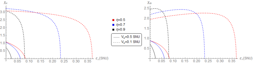
Figure 10: Holevo bound vs excess noise in the squeezed quadrature $\epsilon_{x}$ for RR (left) and DR (right), for an initially pure squeezed state with squeezed quadrature $V_{s}$, attenuated by loss $\eta$. Modulation variance $V_{x}=10$ SNU.

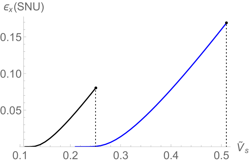
(a)

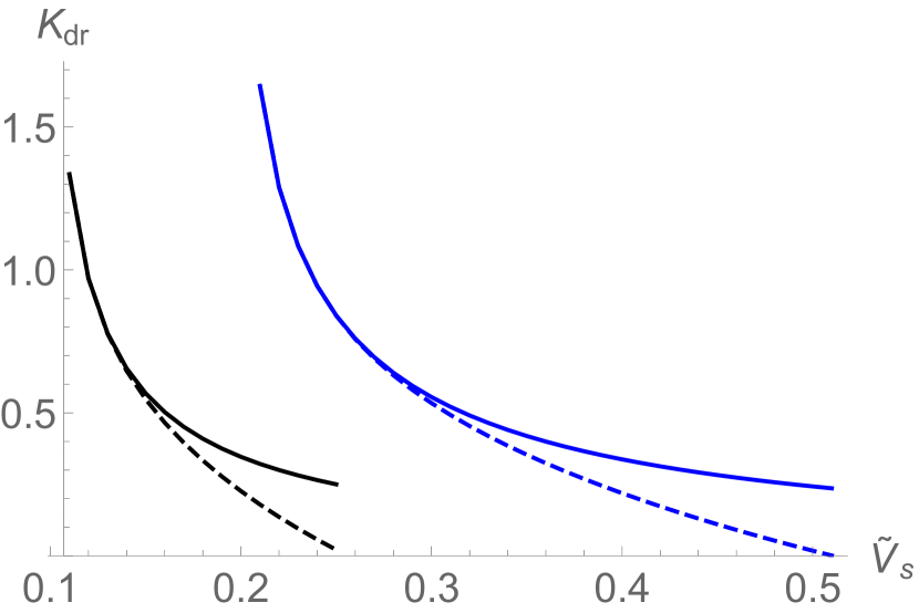
(b)

Figure 11: (a) shows optimal $\epsilon_{x}$ to obtain minimal key rate Eq. 23, for different noisy squeezed state with squeezed quadrature variance $\tilde{V}_{s}$, and AS quadrature variance $\tilde{V}_{AS}=10$ SNU (black) and $\tilde{V}_{AS}=5$ SNU (blue). (b) shows key rates for DR, when optimal noise distribution from (a) is used (dashed) and when all the noise is considered to be in AS quadrature (solid).

Appendix B Parameter estimation

We start by defining $\widehat{C_{AB}}:=\frac{1}{m+n}(\sum^{m}_{i=1}M^{x}_{i}B^{x}_{i}+\sum^{n}_{j=1}M^{p}_{j}B^{p}_{j})$. Here $m$ and $n$ are the number of measurements of $x$ and $p$ quadratures, respectively, used for parameter estimation, $M^{x},M^{p},B^{x}$ and $B^{p}$ are the realizations of Alice’s random number generator corresponding to quadrature variables $(x_{m},p_{m})$ and realizations of Bob’s quadrature variables $(x_{b},p_{b})$, respectively. We can define estimator of transmittance: $\widehat{T}=\frac{1}{(r_{x}V_{x}+r_{p}V_{p})^{2}}(\widehat{C_{AB}})^{2}$, since

$$E[\widehat{C_{AB}}]=\frac{1}{m+n}(mE[x_{m}x_{b}]+nE[p_{m}p_{b}])$$ (24)

$$E[\widehat{C_{AB}}]=\sqrt{T}(\underbrace{m/(m+n)}_{r_{x}}V_{x}+\underbrace{n/(m+n)}_{r_{p}}V_{p})$$ (25)

On the other hand, we have

$$\split Var[\widehat{C_{AB}}]&=\frac{1}{(m+n)^{2}}\left(\sum^{m}_{i=1}Var[M^{x}_{i}B^{x}_{i}]+\sum^{n}_{j=1}Var[M^{p}_{j}B^{p}_{j}]\right)\\ =\frac{1}{(m+n)^{2}}(mVar[x_{m}x_{b}]+nVar[p_{m}p_{b}])\\ =\frac{1}{(m+n)^{2}}[m(T2V_{x}^{2}+V_{x}V_{Nx})+n(T2V_{p}^{2}+V_{p}V_{Np})]\\$$ (26)

where $V_{Nx}=1+T(V+\epsilon-1)$ and $V_{Np}=1+T(1/V+\epsilon+\Delta V_{u}-1)$. As shown in [12], $Var[\widehat{T}]$ is a function of $E[\widehat{C_{AB}}]$ and $Var[\widehat{C_{AB}}]$:

$$\split Var[\hat{T}]&=\frac{2Var[\widehat{C_{AB}}](Var[\widehat{C_{AB}}]+2(E[\widehat{C_{AB}}])^{2})}{(r_{x}V_{x}+r_{p}V_{p})^{4}}\\ =\frac{2Var[\widehat{C_{AB}}]2(E[\widehat{C_{AB}}])^{2}}{(r_{x}V_{x}+r_{p}V_{p})^{4}}+\frac{2(Var[\widehat{C_{AB}}])^{2}}{(r_{x}V_{x}+r_{p}V_{p})^{4}}$$ (27)

Notice that $Var[\widehat{C_{AB}}]$ is of the order of $1/(m+n)^{2}$. For large number of pulses, the second term is significantly small, and the variance of the estimator $\hat{T}$ can be approximated to:

$$Var[\hat{T}]\approx\frac{4T[nV_{p}(V_{Np}+2TV_{p})+mV_{x}(V_{Nx}+2TV_{x})]}{(nV_{p}+mV_{x})^{2}}=:\Upsilon^{2}$$ (28)

The variance of the estimator for the channel noise of squeezed quadrature defined as $\hat{V}_{\epsilon_{x}}=T\epsilon:=\frac{1}{m}\sum^{m}_{i=1}(B^{x}_{i}-\sqrt{\hat{T}}M^{x}_{i})^{2}+\hat{T}(1-V)-1$ can be approximated to:

$$Var[\hat{V}_{\epsilon_{x}}]\approx\frac{2}{m}[1+T(V+\epsilon-1)]^{2}+(1-V)^{2}\Upsilon^{2}=:s_{x}^{2}$$ (29)

The variance of the estimator for the channel noise of AS quadrature $\hat{V}_{\epsilon_{p}}=T(\epsilon+\Delta_{V}^{u}):=\frac{1}{n}\sum^{n}_{i=1}(B^{p}_{i}-\sqrt{\hat{T}}M^{p}_{i})^{2}+\hat{T}(1-1/V)-1$ can be approximated to:

$$Var[\hat{V}_{\epsilon_{p}}]\approx\frac{2}{n}[1+T(1/V+\epsilon+\Delta V_{u}-1)]^{2}+(1-1/V)^{2}\Upsilon^{2}=:s_{p}^{2}$$ (30)

Note that when the source radiates the coherent state and the channel noise is same for both the quadrature ($\Delta V_{u}$) the variance of the estimator $\hat{V}_{\epsilon}$ can be approximated to $Var[V_{\epsilon}]\approx 2(1+V_{\epsilon})^{2}/(m+n)$, by using the channel noise estimator $\hat{V_{\epsilon}}:=\frac{1}{m+n}(\sum^{m}_{i=1}(B^{x}_{i}-\sqrt{\hat{T}}M^{x}_{i})^{2}+\sum^{n}_{i=1}(B^{p}_{i}-\sqrt{\hat{T}}M^{p}_{i})^{2})-1$ .
To account for the trusted AS noise when using AS quadrature for parameter estimation, we incorporate the trusted noise $\Delta V_{t}$ transforming the expressions for standard deviation to

$$\Upsilon^{2}:=\frac{4T[n[V_{p}-\Delta V_{t}](V_{Np}+\Delta V_{t}+2T[V_{p}-\Delta V_{t}])+mV_{x}(V_{Nx}+2TV_{x})]}{[n(V_{p}-\Delta V_{t})+mV_{x}]^{2}}$$ (31)

$$s^{2}_{p}:=\frac{2}{n}[1+T(1/V+\Delta V_{t}+\epsilon+\Delta V_{u}-1)]^{2}+(1-1/V-\Delta V_{t})^{2}\Upsilon^{2}$$ (32)

For the imbalanced heterodyne measurement, the estimators defined above are no longer valid, since the overall estimated transmittance values for the squeezed and AS quadrature are not equal. We further extend the parameter estimation to include an imbalanced heterodyne measurement. We start by defining $\widehat{C^{\prime}_{AB}}:=\frac{1}{m+n}(\sum^{m}_{i=1}M^{x}_{i}B^{x}_{i}/\sqrt{t_{het}}+\sum^{n}_{j=1}M^{p}_{j}B^{p}_{j}/\sqrt{1-t_{het}})$, where $t_{het}$ is the transmittance of the beamsplitter of imbalanced heterodyne measurement. Following the same procedure as above, we find the variance of the estimator $\hat{T}$ can be approximated as

$$Var[\hat{T}]\approx\frac{4T[nV_{p}(V^{\prime}_{Np}+2TV_{p})+mV_{x}(V^{\prime}_{Nx}+2TV_{x})]}{(nV_{p}+mV_{x})^{2}}=:\Upsilon^{2}$$ (33)

Where $V^{\prime}_{Nx}=1/t_{het}+T(V+\epsilon-1)$ and $V^{\prime}_{Np}=1/(1-t_{het})+T(1/V+\epsilon+\Delta V_{u}-1)$.

The estimator of the channel noise for imbalanced heterodyne detection is $\hat{V}_{\epsilon_{x}}:=\frac{1}{m}\sum^{m}_{i=1}(B^{x}_{i}/t_{het}-\sqrt{\hat{T}}M^{x}_{i})^{2}+\hat{T}(1-V)-1$ for $x$-quadrature, and $\hat{V}_{\epsilon_{p}}:=\frac{1}{m}\sum^{m}_{i=1}(B^{p}_{i}/[1-t_{het}]-\sqrt{\hat{T}}M^{p}_{i})^{2}+\hat{T}(1-1/V)-1$ for $p$-quadrature. The variance of which can be approximated as:

$$Var[\hat{V}_{\epsilon_{x}}]\approx\frac{2}{m}[V^{\prime}_{Nx}]^{2}+(1-V)^{2}Var[\hat{T}]$$ (34)

for $x$-quadrature and

$$Var[\hat{V}_{\epsilon_{p}}]\approx\frac{2}{m}[V^{\prime}_{Np}]^{2}+(1-1/V)^{2}Var[\hat{T}]$$ (35)

for $p$-quadrature.

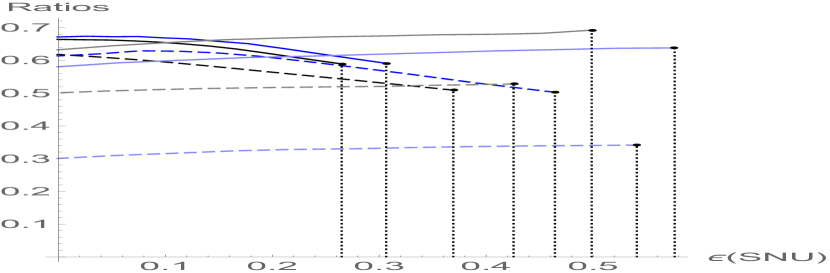
(a)

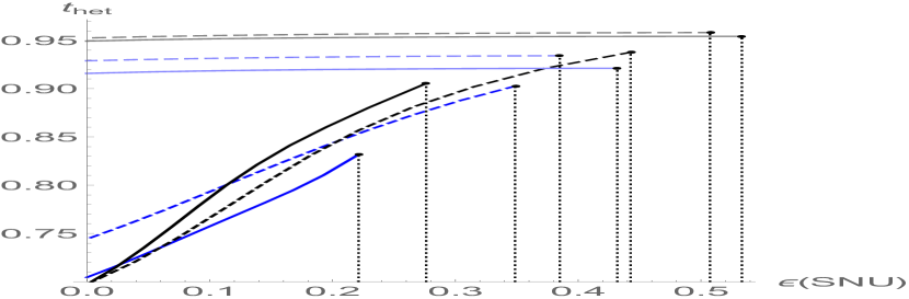
(b)

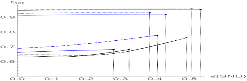
(c)

Figure 12: Optimal ratios of squeezed quadrature measurement for biased homodyne measurement and optimal beamsplitter transmittance $t_{het}$ for the imbalanced heterodyne measurement (used in Fig. 6). Black plots represent a block size of $10^{7}$, blue plots represent a block size of $10^{6}$, solid plots represent a moderately squeezed source state $V=0.5$ SNU, dashed plots represent a highly squeezed source state $V=0.1$ SNU. Light colors correspond to DR, and dark colors correspond to RR. The vertical lines show the maximum tolerable channel noise.

Appendix C

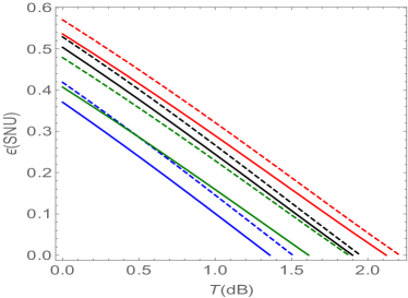
(a)

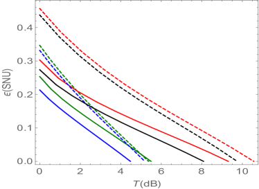
(b)

Figure 13: Tolerance to channel noise for biased homodyne with block size $N=10^{7}$ (red) and $N=10^{6}$ (green), and imbalanced heterodyne measurement with block size $N=10^{7}$ (black) and $N=10^{6}$ (blue), For moderately squeezed source state (solid) and highly squeezed source state (dashed). The modulation variance of the squeezed and AS quadrature $V_{x}$ and $V_{p}$, ratio of squeezed quadrature measurement for biased homodyne detection and the beamsplitter transmittance $t_{het}$ of imbalanced heterodyne measurement are optimised (see Fig. 14 for optimum ratio and transmittance). Reconciliation efficiency $\beta=0.95$

In the main body of the paper, we illustrated the performance of various scenarios in which no measurement results are disclosed for parameter estimation. Here, we show the performance of the scenarios when an optimal amount of measurement results is disclosed to facilitate parameter estimation. Our analysis, depicted in Fig. 13, reveals that biased homodyne measurement consistently outperforms imbalance heterodyne measurement, particularly in terms of tolerable symmetric excess noise.

Exceptionally, imbalance heterodyne measurement surpasses biased homodyne measurement in cases involving elevated antisqueezed noise, a small block size, and substantial squeezing (Fig. 15).

Notably, the optimal ratios of block sizes for parameter estimation and key generation remain relatively constant in the context of DR (Fig. 14). However, for RR, these optimal ratios exhibit variations corresponding to the level of excess noise.

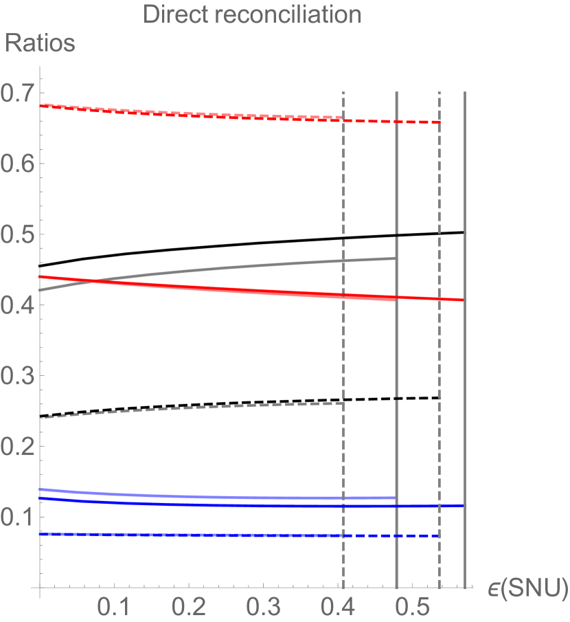
(a)

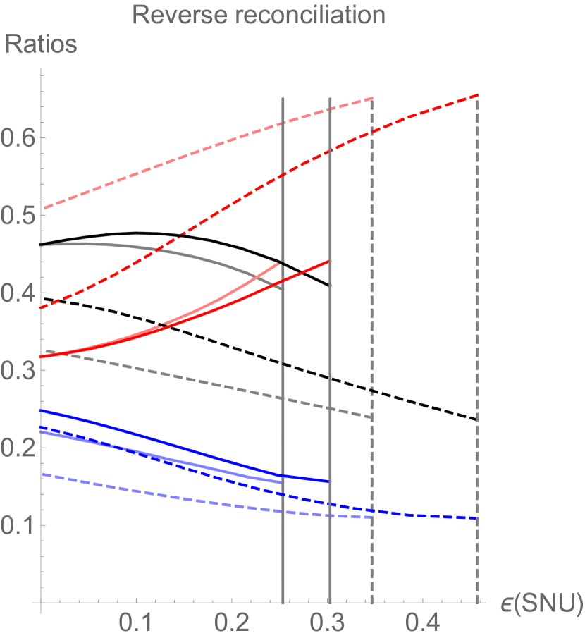
(b)

(c)

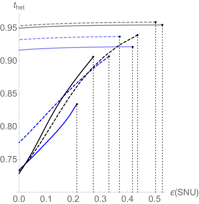
(d)

Figure 14: (a) and (b) show the optimal ratios (used in Fig. 13) for biased homodyne measurement used for key generation $n_{k}/N$ (black), channel noise estimation of AS quadrature $n/N$ (red), and channel noise estimation of squeezed quadrature $m/N$ (blue), for moderately squeezed $V=0.5$ SNU (solid) and highly squeezed $V=0.1$ SNU (dashed) source to achieve maximum distance in the presence of 0.2 SNU AS noise. Darker shades of a color represent a block size of $10^{7}$, and lighter shades represent a block size of $10^{6}$. The gray vertical line shows the maximum tolerable channel noise for the moderately squeezed (dashed) and highly squeezed (solid) source state. (c) and (d) show the optimal transmittance of the beamsplitter of imbalanced heterodyne measurement $t_{het}$, and ratio $n_{k}/N$ of available states used for key generation (used in Fig. 13). Black plots represent a block size of $10^{7}$, blue plots represent a block size of $10^{6}$, solid plots represent a moderately squeezed source state $V=0.5$ SNU, dashed plots represent a highly squeezed source state $V=0.1$ SNU, light colors correspond to DR, and dark colors correspond to RR. The vertical lines show the maximum tolerable channel noise.

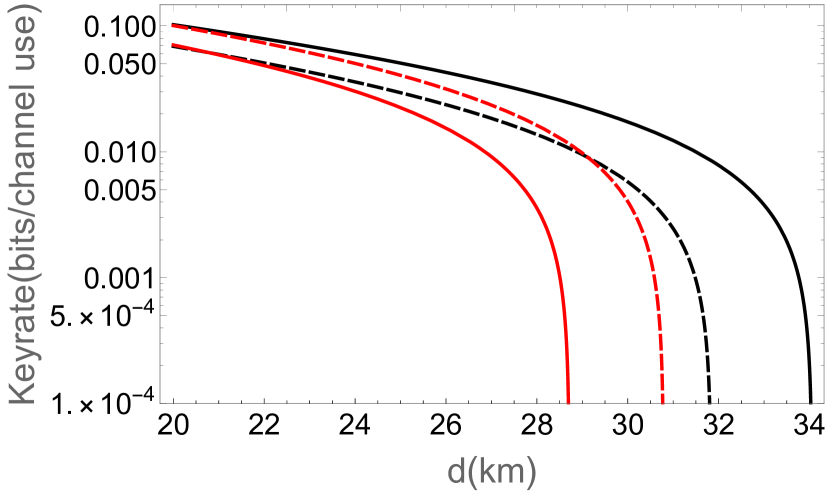
(a) $\Delta V_{t}=0$, $\Delta V_{u}=0$, $N=10^{6}$

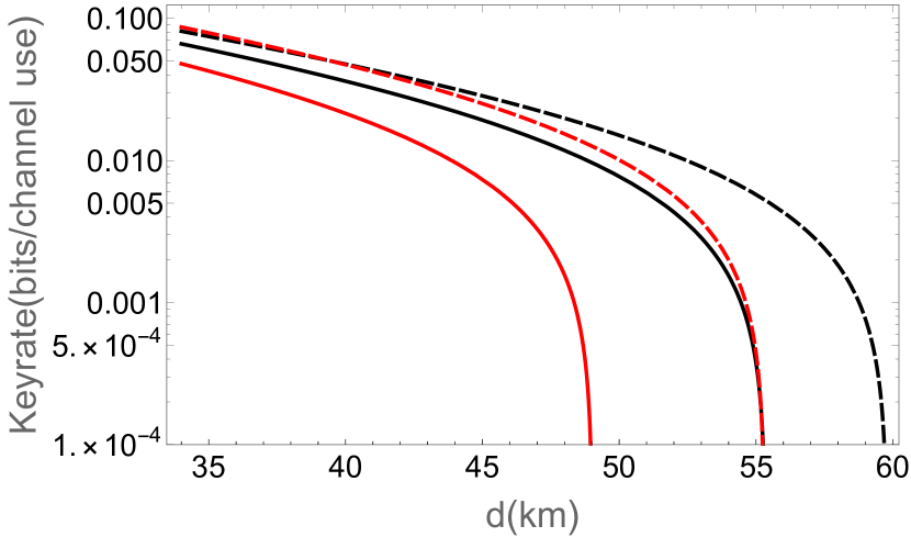
(b) $\Delta V_{t}=0$, $\Delta V_{u}=0$, $N=10^{7}$

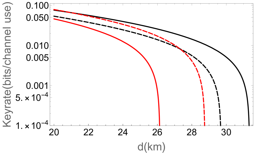
(c) $\Delta V_{t}=0$, $\Delta V_{u}=0.05$, $N=10^{6}$

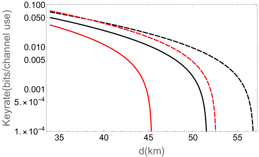
(d) $\Delta V_{t}=0$, $\Delta V_{u}=0.05$, $N=10^{7}$

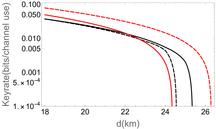
(e) $\Delta V_{t}=5$, $\Delta V_{u}=0$, $N=10^{6}$

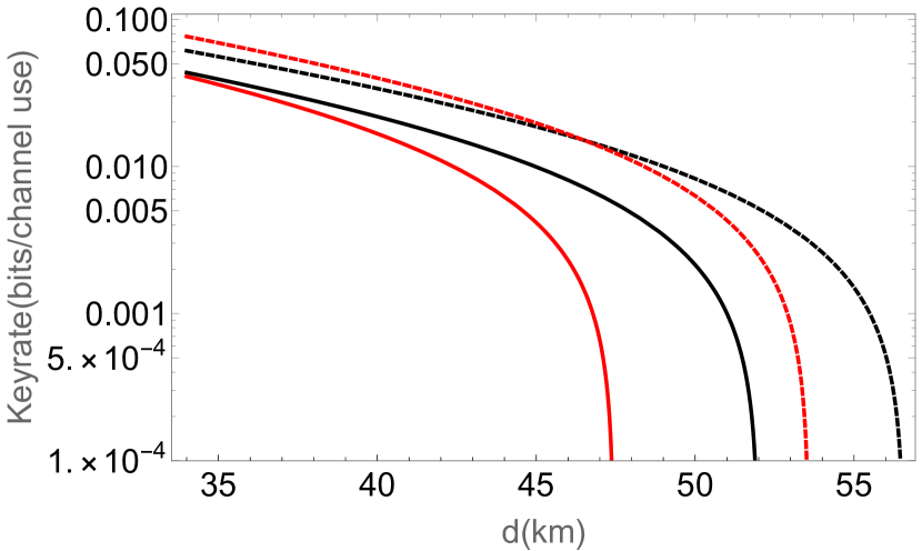
(f) $\Delta V_{t}=5$, $\Delta V_{u}=0$, $N=10^{7}$

Figure 15: Finite-size key rate vs. distance when Bob performs biased homodyne detection (black) and imbalanced heterodyne detection (red), when the parameter estimation requires disclosure of the measurement outcome. The dashed plot represents a highly squeezed source state ($V=0.1$ SNU) and the solid plot represents a moderately squeezed source state ($V=0.5$ SNU). Modulation variances $V_{x}$ and $V_{p}$, transmittance of beamsplitter for heterodyne detection $t_{het}$, ratios of available resources used for key generation $r_{k}$, and parameter estimation $r_{x}$ and $r_{p}$ are optimized. The reconciliation efficiency is $\beta=0.95$, the channel noise is $\epsilon=0.05$ SNU, and the channel attenuation is 0.2 dB/km.

References

- [1] Nicolas Gisin, Grégoire Ribordy, Wolfgang Tittel, and Hugo Zbinden. Quantum cryptography. Reviews of Modern Physics, 74(1):145, 2002.
- [2] Valerio Scarani, Helle Bechmann-Pasquinucci, Nicolas J. Cerf, Miloslav Dušek, Norbert Lütkenhaus, and Momtchil Peev. The security of practical quantum key distribution. Reviews of Modern Physics, 81(3):1301–1350, sep 2009.
- [3] Eleni Diamanti, Hoi-Kwong Lo, Bing Qi, and Zhiliang Yuan. Practical challenges in quantum key distribution. npj Quantum Information, 2:16025, 2016.
- [4] Feihu Xu, Xiongfeng Ma, Qiang Zhang, Hoi-Kwong Lo, and Jian-Wei Pan. Secure quantum key distribution with realistic devices. Reviews of Modern Physics, 92(2):025002, 2020.
- [5] Stefano Pirandola, Ulrik L Andersen, Leonardo Banchi, Mario Berta, Darius Bunandar, Roger Colbeck, Dirk Englund, Tobias Gehring, Cosmo Lupo, Carlo Ottaviani, et al. Advances in quantum cryptography. Advances in Optics and Photonics, 12(4):1012–1236, 2020.
- [6] Samuel L Braunstein and Peter Van Loock. Quantum information with continuous variables. Reviews of Modern Physics, 77(2):513, 2005.
- [7] Frédéric Grosshans and Philippe Grangier. Continuous variable quantum cryptography using coherent states. Physical review letters, 88(5):057902, 2002.
- [8] Frédéric Grosshans, Gilles Van Assche, Jérôme Wenger, Rosa Brouri, Nicolas J Cerf, and Philippe Grangier. Quantum key distribution using gaussian-modulated coherent states. Nature, 421(6920):238–241, 2003.
- [9] Paul Jouguet, Sébastien Kunz-Jacques, Anthony Leverrier, Philippe Grangier, and Eleni Diamanti. Experimental demonstration of long-distance continuous-variable quantum key distribution. Nature photonics, 7(5):378–381, 2013.
- [10] Yichen Zhang, Ziyang Chen, Stefano Pirandola, Xiangyu Wang, Chao Zhou, Binjie Chu, Yijia Zhao, Bingjie Xu, Song Yu, and Hong Guo. Long-distance continuous-variable quantum key distribution over 202.81 km of fiber. Physical review letters, 125(1):010502, 2020.
- [11] Adnan AE Hajomer, Ivan Derkach, Nitin Jain, Hou-Man Chin, Ulrik L Andersen, and Tobias Gehring. Long-distance continuous-variable quantum key distribution over 100 km fiber with local local oscillator. arXiv preprint arXiv:2305.08156, 2023.
- [12] Anthony Leverrier, Frédéric Grosshans, and Philippe Grangier. Finite-size analysis of a continuous-variable quantum key distribution. Phys. Rev. A, 81:062343, Jun 2010.
- [13] Anthony Leverrier. Security of continuous-variable quantum key distribution via a gaussian de finetti reduction. Phys. Rev. Lett., 118:200501, May 2017.
- [14] N. J. Cerf, M. Lévy, and G. Van Assche. Quantum distribution of gaussian keys using squeezed states. Phys. Rev. A, 63:052311, Apr 2001.
- [15] Alexander I Lvovsky. Squeezed light. Photonics: Scientific Foundations, Technology and Applications, 1:121–163, 2015.
- [16] Raúl García-Patrón and Nicolas J. Cerf. Continuous-variable quantum key distribution protocols over noisy channels. Phys. Rev. Lett., 102:130501, Mar 2009.
- [17] L. Madsen, V. Usenko, M. Lassen, and et al. Continuous variable quantum key distribution with modulated entangled states. Nat Commun, 3, Aug 2012.
- [18] Vladyslav C Usenko and Radim Filip. Squeezed-state quantum key distribution upon imperfect reconciliation. New Journal of Physics, 13(11):113007, nov 2011.
- [19] Christian S Jacobsen, Lars S Madsen, Vladyslav C Usenko, Radim Filip, and Ulrik L Andersen. Complete elimination of information leakage in continuous-variable quantum communication channels. npj Quantum Information, 4(1):1–6, 2018.
- [20] Vladyslav C Usenko, Bettina Heim, Christian Peuntinger, Christoffer Wittmann, Christoph Marquardt, Gerd Leuchs, and Radim Filip. Entanglement of gaussian states and the applicability to quantum key distribution over fading channels. New Journal of Physics, 14(9):093048, 2012.
- [21] Ivan Derkach, Vladyslav C Usenko, and Radim Filip. Squeezing-enhanced quantum key distribution over atmospheric channels. New Journal of Physics, 22(5):053006, may 2020.
- [22] Ivan Derkach and Vladyslav C. Usenko. Applicability of squeezed- and coherent-state continuous-variable quantum key distribution over satellite links. Entropy, 23(1), 2021.
- [23] Henning Vahlbruch, Moritz Mehmet, Karsten Danzmann, and Roman Schnabel. Detection of 15 db squeezed states of light and their application for the absolute calibration of photoelectric quantum efficiency. Physical review letters, 117(11):110801, 2016.
- [24] F. Mondain, T. Lunghi, A. Zavatta, E. Gouzien, F. Doutre, M. De Micheli, S. Tanzilli, and V. D’Auria. Chip-based squeezing at a telecom wavelength. Photonics Research, 7(7):A36–A39, July 2019.
- [25] Xiaocong Sun, Yajun Wang, Long Tian, Shaoping Shi, Yaohui Zheng, and Kunchi Peng. Dependence of the squeezing and anti-squeezing factors of bright squeezed light on the seed beam power and pump beam noise. Optics Letters, 44(7):1789–1792, April 2019.
- [26] Takahiro Kashiwazaki, Naoto Takanashi, Taichi Yamashima, Takushi Kazama, Koji Enbutsu, Ryoichi Kasahara, Takeshi Umeki, and Akira Furusawa. Continuous-wave 6-dB-squeezed light with 2.5-THz-bandwidth from single-mode PPLN waveguide. APL Photonics, 5(3):036104, March 2020.
- [27] Karol Łukanowski, Konrad Banaszek, and Marcin Jarzyna. Quantum limits on the capacity of multispan links with phase-sensitive amplification. Journal of Lightwave Technology, pages 1–9, 2023.
- [28] Tobias Gehring, Vitus Händchen, Jörg Duhme, Fabian Furrer, Torsten Franz, Christoph Pacher, Reinhard F Werner, and Roman Schnabel. Implementation of continuous-variable quantum key distribution with composable and one-sided-device-independent security against coherent attacks. Nature communications, 6(1):1–7, 2015.
- [29] Christian Weedbrook, Stefano Pirandola, Raúl García-Patrón, Nicolas J Cerf, Timothy C Ralph, Jeffrey H Shapiro, and Seth Lloyd. Gaussian quantum information. Reviews of Modern Physics, 84(2):621, 2012.
- [30] Ivan Derkach, Vladyslav C Usenko, and Radim Filip. Preventing side-channel effects in continuous-variable quantum key distribution. Physical Review A, 93(3):032309, 2016.
- [31] A. S. Holevo and R. F. Werner. Evaluating capacities of bosonic gaussian channels. Phys. Rev. A, 63:032312, Feb 2001.
- [32] Miguel Navascués, Frédéric Grosshans, and Antonio Acín. Optimality of gaussian attacks in continuous-variable quantum cryptography. Phys. Rev. Lett., 97:190502, Nov 2006.
- [33] Raúl García-Patrón and Nicolas J. Cerf. Unconditional optimality of gaussian attacks against continuous-variable quantum key distribution. Phys. Rev. Lett., 97:190503, Nov 2006.
- [34] A Serafini, M G A Paris, F Illuminati, and S De Siena. Quantifying decoherence in continuous variable systems. Journal of Optics B: Quantum and Semiclassical Optics, 7(4):R19–R36, feb 2005.
- [35] Frédéric Grosshans. Collective attacks and unconditional security in continuous variable quantum keydistribution. Phys. Rev. Lett., 94:020504, Jan 2005.
- [36] Vladyslav C. Usenko and Radim Filip. Trusted noise in continuous-variable quantum key distribution: A threat and a defense. Entropy, 18(1), 2016.
- [37] Hossein Mani, Tobias Gehring, Philipp Grabenweger, Bernhard Ömer, Christoph Pacher, and Ulrik Lund Andersen. Multiedge-type low-density parity-check codes for continuous-variable quantum key distribution. Physical Review A, 103(6):062419, 2021.
- [38] László Ruppert, Vladyslav C. Usenko, and Radim Filip. Long-distance continuous-variable quantum key distribution with efficient channel estimation. Phys. Rev. A, 90:062310, Dec 2014.
- [39] Anthony Leverrier. Composable security proof for continuous-variable quantum key distribution with coherent states. Physical review letters, 114(7):070501, 2015.
- [40] Ruifang Dong, Mikael Lassen, Joel Heersink, Christoph Marquardt, Radim Filip, Gerd Leuchs, and Ulrik L Andersen. Continuous-variable entanglement distillation of non-gaussian mixed states. Physical Review A, 82(1):012312, 2010.
- [41] Michael M Wolf, Geza Giedke, and J Ignacio Cirac. Extremality of gaussian quantum states. Physical review letters, 96(8):080502, 2006.
- [42] D Vasylyev, AA Semenov, and W Vogel. Atmospheric quantum channels with weak and strong turbulence. Physical review letters, 117(9):090501, 2016.