Lightweight Inference for Forward-Forward Algorithm
Abstract
The human brain performs tasks with an outstanding energy-efficiency, i.e., with approximately 20 Watts. The state-of-the-art Artificial/Deep Neural Networks (ANN/DNN), on the other hand, have recently been shown to consume massive amounts of energy. The training of these ANNs/DNNs is done almost exclusively based on the back-propagation algorithm, which is known to be biologically implausible. This has led to a new generation of forward-only techniques, including the Forward-Forward algorithm. In this paper, we propose a lightweight inference scheme specifically designed for DNNs trained using the Forward-Forward algorithm. We have evaluated our proposed lightweight inference scheme in the case of the MNIST and CIFAR datasets, as well as two real-world applications, namely, epileptic seizure detection and cardiac arrhythmia classification using wearable technologies, where complexity overheads/energy consumption is a major constraint, and demonstrate its relevance.
1 Introduction
The state-of-the-art Artificial Neural Networks (ANNs)/Deep Neural Networks (DNNs) consume massive amounts of energy and pose a threat to the environment (Savazzi et al., 2022). A prime example is GPT-3, a Large Language Model (LLM), that consumes over 1000 megawatt-hour for training alone, which is equivalent to a small town’s power consumption for a day (Patterson et al., 2021). The training of these ANNs/DNNs is done almost exclusively based on the back-propagation algorithm, which is known to be biologically implausible (Lillicrap et al., 2016). This has led to a wide range of biologically plausible alternatives, e.g., the Forward-Forward algorithm by (Hinton, 2022), focusing on training DNNs without resorting to the biologically-implausible back-propagation scheme, to bridge the existing performance–efficiency gap between the ANNs/DNNs and the cortex.
The majority of the state-of-the-art studies based on the Forward-Forward algorithm have mainly focused on the training of neural networks. However, the inference over already-trained models also consumes massive amount of energy. Indeed, inference accounts for approximately of the total machine learning energy use at Google (Patterson et al., 2022). This is because the training overheads are per model and often only incurred once, while the inference overheads are per input/usage and, in the long run, the inference overheads may even dominate the overall energy overheads of ANN/DNN, owing to the many-billion-user services that incorporate machine learning.
In this paper, for the first time, we propose a lightweight inference scheme specifically designed for DNNs trained using the Forward-Forward algorithm by (Hinton, 2022). The key insight is that the local energy-based techniques, such as the Forward-Forward algorithm, provide a strong intermediate measure to decide whether the local energy or the goodness in the case of the Forward-Forward algorithm is sufficient to make a confident decision, without the need to complete the entire forward pass. This is inspired by the human nervous system (Saladin, 2009), where the reflexes do not pass directly into the brain, but synapse in the spinal cord, hence without the delay of routing signals through the brain. This is while the complex inputs that require detailed analysis are processed by the brain.
We have evaluated our proposed lightweight inference scheme in the case of the MNIST (LeCun, 1998) and CIFAR (Krizhevsky et al., 2010) datasets and shown that the inference overheads can be reduced by up to 10.4 and 2.2 times, respectively. To demonstrate the relevance of our proposed scheme, we have also evaluated our proposed scheme in the context of two real-world medical applications, namely, epileptic seizure detection using wearable devices (Shoeb, 2009) and cardiac arrhythmia classification using wearable devices (Mark et al., 1982). Wearable technologies are extremely limited in terms of resources, i.e., computing power and energy/battery, and present an excellent application for our proposed lightweight inference to enable real-time and long-term monitoring of patients in ambulatory settings.
2 Related Work
Over the past years, various biologically plausible alternatives have been proposed to address the inherent biologically-implausible nature of back-propagation, e.g., (Lillicrap et al., 2016; Nøkland, 2016; Liao et al., 2016; Schiess et al., 2016; Scellier & Bengio, 2017; Whittington & Bogacz, 2017; Guerguiev et al., 2017; Sacramento et al., 2018; Nøkland & Eidnes, 2019; Meulemans et al., 2021; Millidge et al., 2022; Hinton, 2022; Journé et al., 2022);(Lee et al., 2023); (Dellaferrera et al., 2022); (Chan et al., 2022; Guo et al., 2017).
(Hinton, 2022) proposes one of the recent alternatives for back-propagation, called the Forward-Forward algorithm, which is suitable to be implemented on low-power analog hardware. In the Forward-Forward algorithm, the forward and backward passes of back-propagation are replaced by two forward passes. This algorithm addresses, at least partially, four well-known problems in learning with backpropagation, i.e., weight transport (Grossberg, 1987), non-local weight update (Whittington & Bogacz, 2019), frozen activity (Lillicrap et al., 2020), and update locking (Czarnecki et al., 2017; Jaderberg et al., 2017).
(Dellaferrera et al., 2022) proposes a similar scheme to the Forward-Forward learning, called PEPITA, executing the forward passe twice. In the second forward pass, the input data is modified by the output error of the first forward pass, while the Forward-Forward scheme does not use any feedback. (Journé et al., 2022) also considers two forward passes for the learning procedure and proposes an unsupervised Hebbian-based learning algorithm. Moreover, several very recent studies propose to use the modified versions of the Forward-Forward algorithm for the learning procedure, e.g., (Ororbia & Mali, 2023); (Zhao et al., 2023); (Psenka et al., 2023); (Baghersalimi et al., 2023; Flügel et al., 2023).
Lightweight inference has also been considered in several state-of-the-art studies. Several lightweight inference schemes have been developed both for classical DNNs (Park et al., 2015; Venkataramani et al., 2015; Panda et al., 2016; Georgiev et al., 2017; Bolukbasi et al., 2017; Huang et al., 2023b); (Antorán et al., 2020) and for classical feature-based machine-learning techniques (Sopic et al., 2018a; Forooghifar et al., 2019; Zanetti et al., 2021; Forooghifar et al., 2021; Huang et al., 2023a). For instance, early exit and cascade networks have been proposed to reduce the inference time and energy (Teerapittayanon et al., 2016; Sabokrou et al., 2017; Scardapane et al., 2020; Laskaridis et al., 2021; Matsubara et al., 2022). However, lightweight inference for the forward-only techniques has not been addressed in the state of the art to date. In this work, we bridge this gap and develop the first lightweight inference scheme for neural networks trained based on the forward-only techniques.
3 Lightweight Inference
The intrinsic characteristic of the Forward-Forward algorithm (Hinton, 2022) makes it possible to perform inference without completing a forward pass through all the layers of the network. This can be used to save resources when performing inference operations. In this section, we present an approach for lightweight inference based on the Forward-Forward algorithm.
Inference for a model trained based on the Forward-Forward algorithm can be performed using two different procedures: In the first procedure, for a test sample, we repeat the forward pass operation for all possible labels and calculate the accumulative goodness. We select the label with the highest accumulative goodness. We refer to this procedure as multi-pass, as it requires multiple forward passes. In the second procedure, a softmax layer at the head of the network, which is learned in the training phase, is used to infer based on the activity of layers for a test sample with a neutral label. This is referred to as one-pass, as it requires a single forward pass. Hinton’s one-pass inference process is, in essence, similar to that of the PEPITA algorithm proposed by (Dellaferrera et al., 2022), hence our proposed lightweight inference for the one-pass procedure may also be applied to PEPITA, as we show in Section 4.
3.1 Inference Based on Multi-Pass Procedure
In this part, we focus on the multi-pass inference procedure. In our approach, the network’s training algorithm and architecture are the same as in (Hinton, 2022). For our lightweight inference, however, instead of performing the forward pass through all layers, once the operations for each layer are completed, we inspect the confidence level of the result, and based on that, we decide whether to continue the forward pass. The accumulated goodness up to that layer is used to determine the label.
Figure LABEL:fig:every_label shows our lightweight inference scheme. As illustrated in the figure, after each layer, we check the confidence. The difficulty of the classification task varies from one test sample to another. As shown, the first layer(s) is sufficient for straightforward test samples, while for other samples, more layers may be required.
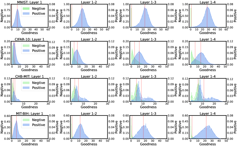
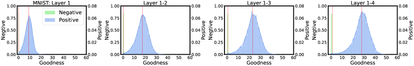
In the Forward-Forward algorithm, we train the model to have high goodness for the positive samples and low goodness for negative ones. Considering this, we use the magnitude of goodness to decide how confident we are about our inference result. The goodness in one layer is the sum of the squared activities, , where is the output of th neuron and is the number of neurons in that layer. For the confidence, we only need to add one single neuron with a sigmoid activation function in each layer whose weights are the activities of that layer and the layers before, and its bias is our confidence threshold. The bias of these neurons is learned based on the validation set. Alternatively, we can calculate and set the bias values based on the mean and standard deviation of the goodness for the validation set. As shown in Fig. 2, the distance between the mean values of the negative and positive samples/distributions increases as we consider more layers.
Next, let us discuss the computational overhead for utilizing one layer of a Forward-Forward network that directly impacts the energy consumption of the platform on which the inference is performed. Suppose our test sample is a vector of length , and we should pass it through a fully connected hidden layer of Rectified Linear Units (ReLUs) with neurons. We show the required computations for calculating the activity vector and the goodness for layer with and , respectively. The overall computation required for a forward pass on layer is . In this case, if our network has hidden layers, the computation required for calculating the goodness for all layers of the network would be . In the case of inference based on the multi-pass procedure, if the data has class labels, then, for each test sample, the computational overhead would be .
In our lightweight inference scheme, we make a trade-off between classification accuracy and computational efficiency (that leads to energy efficiency). As discussed, we define a confidence threshold for every layer determined by the amplitude of accumulated goodness up to that layer based on a validation dataset. The objective would be to increase the classification performance, which could require using more hidden layers, while decreasing the number of layers used for choosing a label, for the sake of computational efficiency.
We show the computation required for the calculation of goodness for one test sample in our lightweight multi-pass inference by . Using our lightweight inference scheme, if we present the probability of completing the inference operation at layer by , then we can show the expected computational overhead for the calculation of goodness for one test sample as follows:
| (1) | ||||
where .111For , we consider . Therefore, we have . As a result, in the worst-case scenario, i.e., when for , , and for , , the computational overhead is the same as the inference procedure in (Hinton, 2022), i.e., .
3.2 Inference Based on One-Pass Procedure
In this part, we focus on the one-pass inference procedure. In general, one-pass inference is more efficient compared to the previous procedure, as instead of passing the test sample with all labels through the network, a test sample is passed through the network once with a neutral label. For our lightweight one-pass inference procedure, instead of only one softmax layer at the head of the network, we train one softmax layer for each hidden layer. The input of each softmax layer is the concatenated activity vectors of all the previous hidden layers. The softmax layers are trained based on train samples with neutral labels (and after all the hidden layers are trained based on positive and negative training samples).
Figure LABEL:fig:one_pass shows our lightweight one-pass inference scheme. The typical configuration of a softmax layer includes calculating the logits and applying the softmax activation function. As the size of the input to the softmax layer increases in each layer by concatenation of activity vectors, the size of the Logit Calculation block correspondingly increases at each layer. These details are visually represented in the figure. After each layer, the activity is passed to its respective softmax layer. We inspect the confidence based on the calculated logits for that softmax layer. As illustrated in the figure, for test samples with less complexity, the first layer(s) is sufficient, but for more complex samples, we continue the forward pass. We incorporate one neuron with a sigmoid activation function in each softmax layer, which is learned based on the validation dataset. The input to this neuron is the maximum logit value for that softmax layer. Alternatively, we can calculate and set the bias values based on the mean and standard deviation of the input values (of confidence neurons) for the validation set.
The computational overhead for the one-pass procedure is slightly different from the previous part. First, we do not pass the test sample times through the network. Second, instead of calculating the goodness of the network’s layers for inference, we pass the output of the layers (activity vector) to the softmax layer. However, calculating the activity of each layer is similar to the previous procedure (shown as for layer ). We show the required computations for the th softmax layer with . The overall computation required for a forward pass on layer is . Assuming our network has hidden layers, making an inference operation by the approach in (Hinton, 2022), requires computational overhead.
We show the computation required for one lightweight one-pass inference operation by . Using our lightweight inference scheme, if we present the probability of completing the inference operation at layer by , then we can show the expected computational overhead for making an inference for one test sample as follows:
| (2) | ||||
where . In the worst-case scenario, i.e., when , is equal to zero, and for , is equal to one, the computational overhead is , which is slightly () worse than the approach in (Hinton, 2022). However, as in most datasets, we have samples with variant complexities, the worst-case scenario is not very likely. The first few layers of the model are sufficient for the majority of samples. We experimentally demonstrate this in Section 4. On the other hand, is usually significantly larger than because, in most cases, the number of neurons in each layer is much larger than the number of classes . Therefore, even if a small proportion of samples use fewer layers, overheads can be compensated.
4 Evaluation
4.1 Experimental Setup
4.1.1 Datasets
To evaluate our lightweight inference scheme, we consider the MNIST dataset of handwritten digits (LeCun, 1998) and the CIFAR-10 dataset of object recognition (Krizhevsky et al., 2010). In addition, we also evaluate our proposed scheme in the context of two real-world medical applications, namely, epilepsy monitoring and seizure detection using wearable technologies based on the CHB-MIT Scalp electroencephalogram (EEG) Dataset (Shoeb, 2009) and cardiac arrhythmia classification using wearable technologies based on the MIT-BIH Arrhythmia Electrocardiogram (ECG) Dataset (Mark et al., 1982), where complexity overhead/energy consumption is a major constraint to ensure real-time and long-term monitoring in ambulatory settings.
MNIST (LeCun, 1998): The MNIST dataset contains handwritten digits, which are grayscale images in 10 different classes (one for each of the 10 digits). We used 50,000 images for training, 10,000 images for validation, and 10,000 images for testing in the inference.
CIFAR-10 (Krizhevsky et al., 2010): The CIFAR-10 dataset is a Computer Vision dataset for object recognition, which consists of color images in 10 different classes. We used 45,000 images for training, 10,000 images for validation, and 5,000 images for testing in the inference.
CHB-MIT Scalp EEG Dataset (Shoeb, 2009): This dataset contains EEG recordings, collected from 22 patients with epilepsy (5 males and 17 females). The recordings are grouped into 23 cases and are divided into seizure and non-seizure classes. To be consistent with wearable IoT devices for real-time seizure monitoring (Sopic et al., 2018b), only the data corresponding to two channels, i.e., T7F7 and T8F8, are considered for the classification. The data corresponding to patients 6, 14, and 16 is eliminated due to their very short-lasting seizures. We use 70%, 15%, and 15% of the dataset for training, validation, and test process, respectively.
MIT-BIH Arrhythmia Dataset (Mark et al., 1982): This dataset encompasses ECG recordings from 47 different patients with cardiovascular problems. Five different types of arrhythmias are categorized by beat annotations (Arlington, 1998). We use the pre-processed data provided in (Kachuee et al., 2018). We consider 70% of data for training, 15% for validation, and 15% to test the model.
4.1.2 Baselines
As discussed previously, we apply our proposed lightweight inference in the context of three state-of-the-art techniques, namely:
- •
- •
-
•
PEPITA (PT), (Dellaferrera et al., 2022): This is the implementation of the algorithm proposed in (Dellaferrera et al., 2022), which is referred to as PEPITA (PT), where the inference process requires only two forward passes. The PEPITA implementation by (Dellaferrera et al., 2022)333https://github.com/GiorgiaD/PEPITA only supports up to 3 hidden layers (Pau & Aymone, 2023).
| Dataset | Layers | Forward-Forward [MP] | Forward-Forward [OP] | PEPITA [PT] | |||
|---|---|---|---|---|---|---|---|
| (Hinton, 2022) | (Hinton, 2022) | (Dellaferrera et al., 2022) | |||||
| MP | Light-MP | OP | Light-OP | PT | Light-PT | ||
| 2 | 1.450.05 | 1.430.04 | 1.450.05 | 1.230.03 | 5.100.51 | 5.100.19 | |
| 3 | 1.400.01 | 1.400.02 | 1.450.09 | 1.060.02 | 4.980.28 | 4.850.09 | |
| MNIST | 4 | 1.510.01 | 1.510.02 | 1.530.10 | 1.020.07 | - | - |
| (LeCun, 1998) | 5 | 1.600.05 | 1.530.01 | 1.570.03 | 1.090.09 | - | - |
| 6 | 1.620.01 | 1.550.02 | 1.570.05 | 0.930.04 | - | - | |
| 2 | 50.990.09 | 46.170.27 | 47.420.26 | 46.560.25 | 61.332.13 | 60.531.97 | |
| 3 | 50.590.09 | 46.120.36 | 47.420.12 | 46.410.32 | 62.132.41 | 62.110.92 | |
| CIFAR-10 | 4 | 50.650.11 | 46.050.30 | 47.780.37 | 46.250.37 | - | - |
| (Krizhevsky et al., 2010) | 5 | 50.370.46 | 45.430.03 | 48.010.17 | 46.300.23 | - | - |
| 6 | 50.750.28 | 45.830.34 | 47.670.23 | 46.060.40 | - | - | |
| 2 | 37.540.53 | 36.220.40 | 36.790.26 | 31.380.54 | 36.081.44 | 31.911.60 | |
| 3 | 37.540.55 | 34.650.93 | 36.220.55 | 28.860.80 | 34.981.88 | 31.200.77 | |
| CHB-MIT | 4 | 39.620.55 | 34.841.45 | 37.980.98 | 28.230.08 | - | - |
| (Shoeb, 2009) | 5 | 38.740.18 | 32.290.82 | 37.291.64 | 25.150.17 | - | - |
| 6 | 39.180.35 | 32.070.53 | 37.290.72 | 24.020.23 | - | - | |
| 2 | 10.820.63 | 10.060.44 | 10.440.08 | 10.130.19 | 16.050.41 | 13.980.50 | |
| 3 | 10.290.16 | 9.680.34 | 10.820.66 | 10.680.29 | 15.190.40 | 14.310.21 | |
| MIT-BIH | 4 | 10.740.97 | 10.070.21 | 10.860.13 | 10.540.14 | - | - |
| (Mark et al., 1982) | 5 | 10.870.18 | 9.840.25 | 10.930.61 | 10.110.21 | - | - |
| 6 | 10.660.04 | 9.540.41 | 10.590.39 | 9.990.12 | - | - | |
| Dataset | Layers | Forward-Forward [MP] | Forward-Forward [OP] | PEPITA [PT] | |||
|---|---|---|---|---|---|---|---|
| (Hinton, 2022) | (Hinton, 2022) | (Dellaferrera et al., 2022) | |||||
| MP | Light-MP | OP | Light-OP | PT | Light-PT | ||
| 2 | 5.31M | 2.18M (1.18) | 5.35M | 1.57M (1.01) | 1.76M | 0.98M (1.22) | |
| 3 | 9.12M | 2.56M (1.28) | 9.18M | 1.61M (1.03) | 2.76M | 1.14M (1.37) | |
| MNIST | 4 | 12.94M | 2.95M (1.38) | 13.01M | 1.65M (1.04) | - | - |
| (LeCun, 1998) | 5 | 16.75M | 3.29M (1.47) | 16.85M | 1.69M (1.05) | - | - |
| 6 | 20.57M | 3.67M (1.57) | 20.68M | 1.73M (1.06) | - | - | |
| 2 | 9.67M | 7.76M (1.49) | 9.71M | 7.47M (1.42) | 4.00M | 3.79M (1.78) | |
| 3 | 13.49M | 9.10M (1.85) | 13.54M | 8.90M (1.79) | 5.00M | 4.55M (2.54) | |
| CIFAR-10 | 4 | 17.30M | 10.31M (2.16) | 17.38M | 10.34M (2.16) | - | - |
| (Krizhevsky et al., 2010) | 5 | 21.12M | 11.55M (2.49) | 21.21M | 11.80M (2.54) | - | - |
| 6 | 24.93M | 12.62M (2.72) | 25.05M | 13.13M (2.89) | - | - | |
| 2 | 5.77M | 4.54M (1.67) | 5.80M | 3.26M (1.33) | 2.00M | 1.17M (1.16) | |
| 3 | 9.58M | 6.26M (2.12) | 9.64M | 4.52M (1.66) | 3.00M | 1.25M (1.25) | |
| CHB-MIT | 4 | 13.39M | 8.39M (2.68) | 13.47M | 5.62M (1.95) | - | - |
| (Shoeb, 2009) | 5 | 17.21M | 10.19M (3.16) | 17.31M | 6.62M (2.21) | - | - |
| 6 | 21.02M | 11.02M (3.38) | 21.14M | 7.43M (2.42) | - | - | |
| 2 | 4.17M | 1.07M (1.18) | 4.21M | 0.71M (1.08) | 1.18M | 0.44M (1.25) | |
| 3 | 7.98M | 1.49M (1.29) | 8.04M | 1.02M (1.16) | 2.18M | 0.73M (1.54) | |
| MIT-BIH | 4 | 11.80M | 1.99M (1.43) | 11.88M | 1.31M (1.24) | - | - |
| (Mark et al., 1982) | 5 | 15.61M | 2.01M (1.43) | 15.71M | 1.59M (1.30) | - | - |
| 6 | 19.43M | 3.06M (1.71) | 19.53M | 1.84M (1.38) | - | - | |
4.1.3 Implementation Details
Our proposed lightweight inference scheme is implemented in PyTorch (Paszke et al., 2019). We have trained all three state-of-the-art algorithms and tested our lightweight inference scheme on the server of -core Intel(R) Xeon(R) Gold 6226R (Skylake) Central Processing Units (CPUs) and 1 NVIDIA Tesla T4 Graphics Processing Cards (GPUs).
For training MP and OP, we consider several scenarios for fully connected networks with a maximum of 6 hidden layers and a maximum of 2,000 neurons for each layer. We also consider the model used by (Hinton, 2022) (4 hidden layers and 2000 neurons for each layer) as the default model in MP and OP. We use the Stochastic Gradient Descent (SGD) optimizer with a learning rate of . We set the batch size to 100 for the MNIST, CIFAR-10, and MIT-BIH datasets. For the CHB-MIT dataset, the personalized model was trained with batch gradient descent. As for other training parameters, we have considered the values according to the Forward-Forward algorithm.
For training PT, we consider the model used by (Srinivasan et al., 2023) (3 hidden layers and 1024 neurons for each layer) as the default model in PT. We use a momentum optimizer with a learning rate of . We set the batch size to 64 for MNIST, CIFAR-10, and MIT-BIH datasets. We set the number of epochs to 100 for all four datasets in MP, OP, and PT. After training, we extract the confidence threshold for each layer based on the validation data.
The datasets in our experiments are balanced, and error, i.e., the total number of incorrectly classified inputs divided by the total number of inputs, is used as the metric of classification performance. We use Multiply–Accumulate Operations (MACs) to evaluate the complexity of inference processes. In addition, each test sample exploits the corresponding number of layers used in lightweight inference. We use the “Mean Layers” to capture the average/mean number of layers used for all the test samples.
4.2 Results
In this section, we evaluate our proposed lightweight inference scheme in terms of prediction performance/error and computational complexity.
4.2.1 Performance Evaluation
In this section, we investigate the performance of our lightweight inference scheme based on MP, OP, and PT. We consider the networks with the same number of neurons (2000 neurons for MP and OP; 1024 neurons for PT) in each hidden layer. We adjust the number of hidden layers from 2 to 6 for MP and OP. We adjust the number of hidden layers from 2 to 3 for PT because PT only supports up to 3 hidden layers (Pau & Aymone, 2023).
Table 1 shows the error comparison between these three state-of-the-art techniques and our lightweight inference scheme. For MP, the Light-MP error is on par with the MP error for MNIST, CIFAR-10, CHB-MIT, and MIT-BIH datasets in different layer settings. Similarly, for OP, the Light-OP error is on par with the OP error for all four datasets. Finally, for PT, the Light-PT error is also comparable to the PT error for all four datasets.444Note that, as shown in (Srinivasan et al., 2023), the overall error marginally increases with the number of layers. We have observed a similar phenomenon in certain cases for the Forward-Forward algorithm by (Hinton, 2022).
In summary, our lightweight inference achieves a comparable classification error and even a smaller error in some cases.
4.2.2 Complexity Evaluation
In this section, we evaluate the complexity of our lightweight inference scheme based on MP, OP, and PT. First, we refer to the same experimental settings in Table 1 and report the MACs and Mean Layers (shown in parentheses) used by our lightweight inference scheme in Table 2. For Light-MP, Light-OP, and Light-PT evaluated on MNIST, CIFAR-10, CHB-MIT, and MIT-BIH datasets, the value of Mean Layers used in our lightweight inference scheme is always significantly lower than the number of the network layers.
| Dataset | Layers | FF [MP] | FF [OP] | ||
|---|---|---|---|---|---|
| MP | Light-MP | OP | Light-OP | ||
| 2 | 6.58 | 2.24 | 0.72 | 0.30 | |
| 3 | 14.77 | 3.25 | 1.40 | 0.31 | |
| MNIST | 4 | 22.81 | 3.39 | 2.30 | 0.32 |
| 5 | 29.70 | 4.22 | 3.06 | 0.34 | |
| 6 | 36.73 | 5.52 | 3.75 | 0.36 | |
| 2 | 14.85 | 10.38 | 1.39 | 1.15 | |
| 3 | 22.32 | 13.19 | 2.20 | 1.47 | |
| CIFAR-10 | 4 | 29.57 | 16.38 | 2.98 | 1.76 |
| 5 | 35.83 | 17.45 | 3.36 | 2.01 | |
| 6 | 42.38 | 19.50 | 4.31 | 2.24 | |
| 2 | 1.55 | 1.19 | 0.77 | 0.53 | |
| 3 | 3.42 | 1.94 | 1.42 | 0.76 | |
| CHB-MIT | 4 | 4.73 | 2.85 | 2.28 | 1.01 |
| 5 | 6.02 | 3.51 | 3.44 | 1.21 | |
| 6 | 7.33 | 3.74 | 3.72 | 1.36 | |
| 2 | 2.56 | 0.88 | 0.58 | 0.23 | |
| 3 | 6.83 | 1.36 | 1.18 | 0.28 | |
| MIT-BIH | 4 | 11.26 | 1.83 | 1.95 | 0.34 |
| 5 | 14.46 | 1.87 | 2.88 | 0.41 | |
| 6 | 18.03 | 2.90 | 3.49 | 0.44 | |
Similarly, the MACs of Light-MP, Light-OP, and Light-PT are always significantly lower than the MACs of MP, OP, and PT, respectively, for all four datasets in different layer settings. However, as the number of network layers increases from 2 to 6 for MP and OP, and from 2 to 3 for PT, the Mean Layers used tend to increase but the relative percentage of layers used decreases. Moreover, we have conducted experiments to show the actual execution time reduction of our lightweight inference scheme, on a MacBook Pro with the Apple M1 pro CPU and 32 GB of RAM. Table 3 presents the improvement of our scheme against the Forward-Forward algorithm. Taking MNIST with 4 layers as an example, the execution time of FF [MP], i.e., 22.81 ms, is reduced by a factor of to 3.39 ms, and the execution time of FF [OP], i.e., 2.30 ms, by a factor of to 0.32 ms.
4.2.3 Detailed Analysis and Discussion
To show the relevance of our lightweight inference scheme for the new generation of forward-only techniques, we further analyze our proposed lightweight inference scheme for neural networks trained based on MP, OP, and PT.
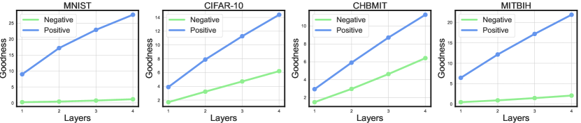
Let us first investigate the distance between the negative data and the positive data for the four datasets considered in this work. Here, we calculate the mean values of the negative data and positive data for MNIST, CIFAR-10, CHB-MIT, and MIT-BIH datasets. These mean values are in consecutive layers based on MP. As shown in Fig. 3, the distance between the mean values of the negative and positive data increases as we consider more layers. The figure shows that a higher confidence level is attained as more layers are taken into account.
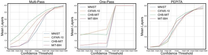
Next, we investigate the relationship between the Mean Layers and the confidence threshold to show the computational efficiency of our proposed lightweight inference scheme. We conduct seven experiments separately with different confidence thresholds for the lightweight inference schemes based on MP, OP, and PT for their default model. At each layer, we extract the mean and std from validation data and then use the threshold for confidence measurement. The different confidence thresholds range from to . As shown in Fig 4, if the confidence threshold increases, the mean number of layers used increases accordingly. The reason is that a higher confidence threshold means that fewer test samples in the inference process are regarded as confident and need to be passed to the next layers. Hence, our lightweight inference scheme provides the possibility to achieve different levels of computational efficiency for different confidence thresholds.
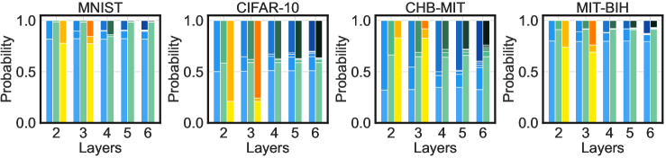
Finally, we also investigated the probability of the number of layers used for Light-MP, Light-OP, and Light-PT. Towards this, we extract the probability of each layer used for all the test data based on confidence. We refer to the same experimental settings in Table 1. Fig 5 shows the probability of the number of layers used in the proposed schemes. We use the lightest color to represent one layer and the darkest color to represent six layers. For the MNIST dataset, more than 77% of the test samples are confident just at the first layer, for Light-MP, Light-OP, and Light-PT considering different number of layers. For CIFAR-10 datasets, more than 50% of the test samples are confident at the first layer for Light-MP and Light-OP with different numbers of layers. For CHB-MIT and MIT-BIH datasets, respectively, more than 32% and 69% of the test samples are confident at the first layer for our proposed lightweight inference scheme based on MP, OP, and PT. Fig 5 shows that by considering confidence, our lightweight inference scheme decreases the mean number of layers used in inference.
5 Conclusions
In this paper, we propose a lightweight inference scheme based on the new generation of forward-only techniques, measuring the confidence at each layer. This lightweight inference scheme aims for computational efficiency in the inference of these forward-only DNNs. We have evaluated our lightweight inference scheme on the Forward-Forward Multi-Pass (Hinton, 2022), One-Pass (Hinton, 2022), and PEPITA (Dellaferrera et al., 2022), based on the MNIST, CIFAR-10, CHB-MIT, and MIT-BIH datasets. The results show that our lightweight inference scheme achieves computational efficiency by decreasing the number of layers used in inference, with a comparable classification error.
References
- Antorán et al. (2020) Antorán, J., Allingham, J., and Hernández-Lobato, J. M. Depth uncertainty in neural networks. Advances in neural information processing systems, 33:10620–10634, 2020.
- Arlington (1998) Arlington, V. Testing and reporting performance results of cardiac rhythm and st segment measurement algorithms. ANSI-AAMI EC57, 1998.
- Baghersalimi et al. (2023) Baghersalimi, S., Amirshahi, A., Teijeiro, T., Aminifar, A., and Atienza Alonso, D. Layer-wise learning framework for efficient dnn deployment in biomedical wearable systems. [Proceedings of IEEE BSN 2023], 2023.
- Bolukbasi et al. (2017) Bolukbasi, T., Wang, J., Dekel, O., and Saligrama, V. Adaptive neural networks for efficient inference. In International Conference on Machine Learning, pp. 527–536. PMLR, 2017.
- Chan et al. (2022) Chan, K. H. R., Yu, Y., You, C., Qi, H., Wright, J., and Ma, Y. Redunet: A white-box deep network from the principle of maximizing rate reduction. The Journal of Machine Learning Research, 23(1):4907–5009, 2022.
- Czarnecki et al. (2017) Czarnecki, W. M., Świrszcz, G., Jaderberg, M., Osindero, S., Vinyals, O., and Kavukcuoglu, K. Understanding synthetic gradients and decoupled neural interfaces. In International Conference on Machine Learning, pp. 904–912. PMLR, 2017.
- Dellaferrera et al. (2022) Dellaferrera, G. et al. Error-driven input modulation: solving the credit assignment problem without a backward pass. In International Conference on Machine Learning, pp. 4937–4955. PMLR, 2022.
- Flügel et al. (2023) Flügel, K., Coquelin, D., Weiel, M., Debus, C., Streit, A., and Götz, M. Feed-forward optimization with delayed feedback for neural networks. arXiv preprint arXiv:2304.13372, 2023.
- Forooghifar et al. (2019) Forooghifar, F., Aminifar, A., Cammoun, L., Wisniewski, I., Ciumas, C., Ryvlin, P., and Atienza, D. A self-aware epilepsy monitoring system for real-time epileptic seizure detection. In ACM/Springer Mobile Networks and Applications (MONET). ACM/Springer, 2019.
- Forooghifar et al. (2021) Forooghifar, F., Aminifar, A., Teijeiro, T., Aminifar, A., Jeppesen, J., Beniczky, S., and Atienza, D. Self-aware anomaly-detection for epilepsy monitoring on low-power wearable electrocardiographic devices. In 2021 IEEE 3rd International Conference on Artificial Intelligence Circuits and Systems (AICAS), pp. 1–4. IEEE, 2021.
- Georgiev et al. (2017) Georgiev, P., Bhattacharya, S., Lane, N. D., and Mascolo, C. Low-resource multi-task audio sensing for mobile and embedded devices via shared deep neural network representations. Proceedings of the ACM on Interactive, Mobile, Wearable and Ubiquitous Technologies, 1(3):1–19, 2017.
- Grossberg (1987) Grossberg, S. Competitive learning: From interactive activation to adaptive resonance. Cognitive science, 11(1):23–63, 1987.
- Guerguiev et al. (2017) Guerguiev, J., Lillicrap, T. P., and Richards, B. A. Towards deep learning with segregated dendrites. Elife, 6:e22901, 2017.
- Guo et al. (2017) Guo, C., Pleiss, G., Sun, Y., and Weinberger, K. Q. On calibration of modern neural networks. In International conference on machine learning, pp. 1321–1330. PMLR, 2017.
- Hinton (2022) Hinton, G. The forward-forward algorithm: Some preliminary investigations. arXiv preprint arXiv:2212.13345, 2022.
- Huang et al. (2023a) Huang, B., Abtahi, A., and Aminifar, A. Lightweight machine learning for seizure detection on wearable devices. In ICASSP 2023-2023 IEEE International Conference on Acoustics, Speech and Signal Processing (ICASSP), pp. 1–2. IEEE, 2023a.
- Huang et al. (2023b) Huang, B., Zanetti, R., Abtahi, A., Atienza, D., and Aminifar, A. Epilepsynet: Interpretable self-supervised seizure detection for low-power wearable systems. In 2023 IEEE 5th International Conference on Artificial Intelligence Circuits and Systems (AICAS), pp. 1–5. IEEE, 2023b.
- Jaderberg et al. (2017) Jaderberg, M., Czarnecki, W. M., Osindero, S., Vinyals, O., Graves, A., Silver, D., and Kavukcuoglu, K. Decoupled neural interfaces using synthetic gradients. In International conference on machine learning, pp. 1627–1635. PMLR, 2017.
- Journé et al. (2022) Journé, A., Rodriguez, H. G., Guo, Q., and Moraitis, T. Hebbian deep learning without feedback. arXiv preprint arXiv:2209.11883, 2022.
- Kachuee et al. (2018) Kachuee, M., Fazeli, S., and Sarrafzadeh, M. Ecg heartbeat classification: A deep transferable representation. In 2018 IEEE international conference on healthcare informatics (ICHI), pp. 443–444. IEEE, 2018.
- Krizhevsky et al. (2010) Krizhevsky, A., Nair, V., and Hinton, G. Cifar-10 (canadian institute for advanced research). URL http://www. cs. toronto. edu/kriz/cifar. html, 5(4):1, 2010.
- Laskaridis et al. (2021) Laskaridis, S., Kouris, A., and Lane, N. D. Adaptive inference through early-exit networks: Design, challenges and directions. In Proceedings of the 5th International Workshop on Embedded and Mobile Deep Learning, pp. 1–6, 2021.
- LeCun (1998) LeCun, Y. The mnist database of handwritten digits. http://yann. lecun. com/exdb/mnist/, 1998.
- Lee et al. (2023) Lee, J. H., Haghighatshoar, S., and Karbasi, A. Exact gradient computation for spiking neural networks via forward propagation. In International Conference on Artificial Intelligence and Statistics, pp. 1812–1831. PMLR, 2023.
- Liao et al. (2016) Liao, Q., Leibo, J., and Poggio, T. How important is weight symmetry in backpropagation? In Proceedings of the AAAI Conference on Artificial Intelligence, volume 30, 2016.
- Lillicrap et al. (2016) Lillicrap, T. P., Cownden, D., Tweed, D. B., and Akerman, C. J. Random synaptic feedback weights support error backpropagation for deep learning. Nature communications, 7(1):13276, 2016.
- Lillicrap et al. (2020) Lillicrap, T. P., Santoro, A., Marris, L., Akerman, C. J., and Hinton, G. Backpropagation and the brain. Nature Reviews Neuroscience, 21(6):335–346, 2020.
- Mark et al. (1982) Mark, R., Schluter, P., Moody, G., Devlin, P., and Chernoff, D. An annotated ecg database for evaluating arrhythmia detectors. In IEEE Transactions on Biomedical Engineering, volume 29, pp. 600–600, 1982.
- Matsubara et al. (2022) Matsubara, Y., Levorato, M., and Restuccia, F. Split computing and early exiting for deep learning applications: Survey and research challenges. ACM Computing Surveys, 55(5):1–30, 2022.
- Meulemans et al. (2021) Meulemans, A., Tristany Farinha, M., García Ordóñez, J., Vilimelis Aceituno, P., Sacramento, J., and Grewe, B. F. Credit assignment in neural networks through deep feedback control. Advances in Neural Information Processing Systems, 34:4674–4687, 2021.
- Millidge et al. (2022) Millidge, B., Tschantz, A., and Buckley, C. L. Predictive coding approximates backprop along arbitrary computation graphs. Neural Computation, 34(6):1329–1368, 2022.
- Nøkland (2016) Nøkland, A. Direct feedback alignment provides learning in deep neural networks. Advances in neural information processing systems, 29, 2016.
- Nøkland & Eidnes (2019) Nøkland, A. and Eidnes, L. H. Training neural networks with local error signals. In International conference on machine learning, pp. 4839–4850. PMLR, 2019.
- Ororbia & Mali (2023) Ororbia, A. and Mali, A. The predictive forward-forward algorithm. arXiv preprint arXiv:2301.01452, 2023.
- Panda et al. (2016) Panda, P., Sengupta, A., and Roy, K. Conditional deep learning for energy-efficient and enhanced pattern recognition. In 2016 Design, Automation & Test in Europe Conference & Exhibition (DATE), pp. 475–480. IEEE, 2016.
- Park et al. (2015) Park, E., Kim, D., Kim, S., Kim, Y.-D., Kim, G., Yoon, S., and Yoo, S. Big/little deep neural network for ultra low power inference. In 2015 International Conference on Hardware/Software Codesign and System Synthesis (CODES+ ISSS), pp. 124–132. IEEE, 2015.
- Paszke et al. (2019) Paszke, A., Gross, S., Massa, F., Lerer, A., Bradbury, J., Chanan, G., Killeen, T., Lin, Z., Gimelshein, N., Antiga, L., et al. Pytorch: An imperative style, high-performance deep learning library. Advances in neural information processing systems, 32, 2019.
- Patterson et al. (2021) Patterson, D., Gonzalez, J., Le, Q., Liang, C., Munguia, L.-M., Rothchild, D., So, D., Texier, M., and Dean, J. Carbon emissions and large neural network training, 2021.
- Patterson et al. (2022) Patterson, D., Gonzalez, J., Hölzle, U., Le, Q., Liang, C., Munguia, L.-M., Rothchild, D., So, D. R., Texier, M., and Dean, J. The carbon footprint of machine learning training will plateau, then shrink. Computer, 55(7):18–28, 2022. doi: 10.1109/MC.2022.3148714.
- Pau & Aymone (2023) Pau, D. P. and Aymone, F. M. Suitability of forward-forward and pepita learning to mlcommons-tiny benchmarks. In 2023 IEEE International Conference on Omni-layer Intelligent Systems (COINS), pp. 1–6. IEEE, 2023.
- Psenka et al. (2023) Psenka, M., Pai, D., Raman, V., Sastry, S., and Ma, Y. Representation learning via manifold flattening and reconstruction. arXiv preprint arXiv:2305.01777, 2023.
- Sabokrou et al. (2017) Sabokrou, M., Fayyaz, M., Fathy, M., and Klette, R. Deep-cascade: Cascading 3d deep neural networks for fast anomaly detection and localization in crowded scenes. IEEE Transactions on Image Processing, 26(4):1992–2004, 2017.
- Sacramento et al. (2018) Sacramento, J., Ponte Costa, R., Bengio, Y., and Senn, W. Dendritic cortical microcircuits approximate the backpropagation algorithm. Advances in neural information processing systems, 31, 2018.
- Saladin (2009) Saladin, K. Anatomy & Physiology: The Unity of Form and Function. McGraw-Hill Higher Education, 2009. ISBN 9780071283410. URL https://books.google.se/books?id=pByBGQAACAAJ.
- Savazzi et al. (2022) Savazzi, S., Rampa, V., Kianoush, S., and Bennis, M. An energy and carbon footprint analysis of distributed and federated learning. IEEE Transactions on Green Communications and Networking, 2022.
- Scardapane et al. (2020) Scardapane, S., Scarpiniti, M., Baccarelli, E., and Uncini, A. Why should we add early exits to neural networks? Cognitive Computation, 12(5):954–966, 2020.
- Scellier & Bengio (2017) Scellier, B. and Bengio, Y. Equilibrium propagation: Bridging the gap between energy-based models and backpropagation. Frontiers in computational neuroscience, 11:24, 2017.
- Schiess et al. (2016) Schiess, M., Urbanczik, R., and Senn, W. Somato-dendritic synaptic plasticity and error-backpropagation in active dendrites. PLoS computational biology, 12(2):e1004638, 2016.
- Shoeb (2009) Shoeb, A. H. Application of machine learning to epileptic seizure onset detection and treatment. PhD thesis, Massachusetts Institute of Technology, 2009.
- Sopic et al. (2018a) Sopic, D., Aminifar, A., Aminifar, A., and Atienza, D. Real-time event-driven classification technique for early detection and prevention of myocardial infarction on wearable systems. In IEEE Transactions on Biomedical Circuits and Systems, 2018a.
- Sopic et al. (2018b) Sopic, D., Aminifar, A., and Atienza, D. e-glass: A wearable system for real-time detection of epileptic seizures. In 2018 IEEE International Symposium on Circuits and Systems (ISCAS), pp. 1–5. IEEE, 2018b.
- Srinivasan et al. (2023) Srinivasan, R. F., Mignacco, F., Sorbaro, M., Refinetti, M., Cooper, A., Kreiman, G., and Dellaferrera, G. Forward learning with top-down feedback: Empirical and analytical characterization. arXiv preprint arXiv:2302.05440, 2023.
- Teerapittayanon et al. (2016) Teerapittayanon, S., McDanel, B., and Kung, H.-T. Branchynet: Fast inference via early exiting from deep neural networks. In 2016 23rd international conference on pattern recognition (ICPR), pp. 2464–2469. IEEE, 2016.
- Venkataramani et al. (2015) Venkataramani, S., Raghunathan, A., Liu, J., and Shoaib, M. Scalable-effort classifiers for energy-efficient machine learning. In Proceedings of the 52nd Annual Design Automation Conference, pp. 1–6, 2015.
- Whittington & Bogacz (2017) Whittington, J. C. and Bogacz, R. An approximation of the error backpropagation algorithm in a predictive coding network with local hebbian synaptic plasticity. Neural computation, 29(5):1229–1262, 2017.
- Whittington & Bogacz (2019) Whittington, J. C. and Bogacz, R. Theories of error back-propagation in the brain. Trends in cognitive sciences, 23(3):235–250, 2019.
- Zanetti et al. (2021) Zanetti, R., Arza, A., Aminifar, A., and Atienza, D. Real-time eeg-based cognitive workload monitoring on wearable devices. IEEE Transactions on Biomedical Engineering, 69(1):265–277, 2021.
- Zhao et al. (2023) Zhao, G., Wang, T., Li, Y., Jin, Y., Lang, C., and Ling, H. The cascaded forward algorithm for neural network training. arXiv preprint arXiv:2303.09728, 2023.
Appendix A Appendix: confidence Level at Different Layers
We investigate the confidence level of MNIST, CIFAR-10, CHB-MIT, and MIT-BIH datasets based on the Forward-Forward algorithm. Fig. 6 illustrates the distribution of validation data (Green: Negative data; Blue: Positive data) and the corresponding mean values (red vertical lines) in the Forward-Forward algorithm for MNIST, CIFAR-10, CHB-MIT, and MIT-BIH datasets. As shown in this figure, the distance between the mean values of the negative and positive samples/distributions increases as we consider more layers.