Novelty Heuristics, Multi-Queue Search, and Portfolios for Numeric Planning

Abstract

Heuristic search is a powerful approach for solving planning problems and numeric planning is no exception. In this paper, we boost the performance of heuristic search for numeric planning with various powerful techniques orthogonal to improving heuristic informedness: numeric novelty heuristics, the Manhattan distance heuristic, and exploring the use of multi-queue search and portfolios for combining heuristics.

1 Introduction

Numeric planning is an expressive extension of classical planning where states are able to exhibit real-valued variables. It was formalised in PDDL2.1 (Fox and Long 2003) and is undecidable in the general case (Helmert 2002). However, it is PSPACE-complete when variables are integer and bounded, and there also exist compilations from numeric to classical planning with certain features that preserve plan length (Gigante and Scala 2023). Similarly to classical planning, the two main approaches for solving numeric planning problems in the literature consist in either heuristic search or compilation into a sequence of satisfiability problems for constraint-based solvers. A recent SAT Modulo Theory (SMT) approach, Patty, has been proposed (Cardellini, Giunchiglia, and Maratea 2024) which provably encodes fewer variables and constraints than previous constraint-based approaches (Scala et al. 2016b; Bofill, Espasa, and Villaret 2017). Compared to heuristic search, it provides better performance on highly numeric planning problems which do not require long plans.

On the other hand, the state of the art for heuristic search in numeric planning still consists of a search with a single heuristic derived from a relaxation of the problem. Such heuristics include the numeric extensions of classical planning heuristics: metric FF (Hoffmann 2002, 2003), LP-based heuristics for computing tighter bounds on the relaxed planning graph (Coles et al. 2008), interval-based, subgoaling, and set-additive derivations of $h^{\text{add}}$ (Scala, Haslum, and Thiébaux 2016; Scala et al. 2016a, 2020a, 2020b), landmarks (Scala et al. 2017), admissible IP-based heuristics (Piacentini et al. 2018), LM-cut and operator counting heuristics (Kuroiwa et al. 2021, 2022; Kuroiwa, Shleyfman, and Beck 2023). Alternatively, Illanes and McIlraith (2017) use a partial policy computed from an abstraction of numeric planning into classical planning for search guidance. Other techniques orthogonal to defining new heuristics for numeric planning also exist, such as abstracting linear numeric problems into simple numeric problems, enabling the use of simple numeric heuristics (Li et al. 2018), and computing state space symmetries with the numeric problem description graph (Shleyfman, Kuroiwa, and Beck 2023).

In this paper, we boost the performance of heuristic search for numeric planners in several orthogonal directions by porting search techniques from classical planning. This includes (1) formalising novelty heuristics for numeric planning, (2) constructing the simple but effective Manhattan distance heuristic, (3) extending the ENHSP planner (Scala et al. 2020b) with multi-queue search, and (4) building naive portfolios. We provide a systematic set of experiments that demonstrate the effectiveness of these approaches on the Numeric Track of the 2023 International Planning Competition (NT-IPC) (Arxer and Scala 2023) and highlight the complementary nature of heuristic search and constraint-based approaches for numeric planning.

2 Background

A numeric planning task (Fox and Long 2003) is given by a tuple $\Pi=\left<X_{p},X_{n},A,s_{0},G\right>$ where $X_{p}$ is a finite set of Boolean variables with domains $\left\{\top,\bot\right\}$ and $X_{n}$ is a finite set of numeric variables with domains $\mathbb{R}$. Let $X=X_{p}\cup X_{n}$ denote the set of state variables. Let $S$ denote the set of possibly infinitely many states in $\Pi$, where a state is a total assignment to Boolean and numeric variables. Let $s_{0}\in S$ be the initial state. A propositional condition is a positive literal, and a numeric condition has the form $\xi\unrhd 0$ where $\xi$ is an arithmetic expression over numeric variables and $\unrhd\in\left\{\geq,>,=\right\}$. Let $[x]^{s}$ and $[\xi]^{s}$ denote the value of $x$ and $\xi$ in $s$, respectively. The goal condition $G$ is a set of propositional and numeric conditions, and we say that a state $s$ satisfies $G$ if $s$ satisfies all conditions in $G$. An action $a$ consists of preconditions and effects. Action preconditions $\operatorname*{pre}(a)$ are sets of propositional and numeric conditions, and action effects $\operatorname*{eff}(a)$ assign Boolean values to Boolean variables, and assign the value of a numeric variable using an arithmetic expression. An action $a$ is applicable in a state $s$ if $s$ satisfies $\operatorname*{pre}(a)$, in which case its successor $a(s)$ is the state where the effects $\operatorname*{eff}(a)$ are applied to the variables in state $s$. If $a$ is not applicable in $s$, we set $a(s)=s_{\bot}\not\in S$. A plan for a numeric planning task is a sequence of actions $a_{1},\ldots,a_{n}$ such that $s_{i}=a_{i}(s_{i-1})\not=s_{\bot}$ for all $1\leq i\leq n$ and $s_{n}$ satisfies $G$. A numeric planning task is solvable if there exists a plan for it.

3 Boosting Search for Numeric Planning

In this section, we outline various techniques to boost the performance of satisficing numeric planning solvers. Firstly, we extend and combine novelty heuristics into a single framework for numeric planning. We then introduce a simple extension of the goal count heuristic for numeric planning which outperforms more sophisticated numeric planning heuristics for single queue search. Lastly, we make use of multi-queue search and portfolios for numeric planning.

3.1 Numeric Novelty Heuristics

Let ${S^{<\mathbb{N}}}$ denote the set of all finite sequences of states in a numeric planning task, and $\left<T\right>$ a finite sequence of states. We write $T_{k}$ for the state of index $k$ in $\left<T\right>$, and $\left<T\right>.s$ for the sequence obtained by appending state $s$ at the end of $\left<T\right>$. Moreover, let $\left<T\right>[:s]$ stand for the substring of $\left<T\right>$ that ends in the element before $s$, and $\left<T_{=h(s)}\right>$ for the substring of $\left<T\right>$ consisting of the states $s^{\prime}$ such that $h(s^{\prime})=h(s)$, where $h$ is a heuristic function. We also assume an enumeration $x_{1},\ldots,x_{N}$ of variables in $X$, where $N=\left|X\right|$.

Definition 3.1 (Novelty Feature).

A novelty feature is a function $f:{S^{<\mathbb{N}}}\times S\to(\mathbb{R}\cup\left\{\bot\right\})^{N}$.

We provide two examples of novelty features for numeric planning. The first example is the assignment feature A, which has been explored in the context of control systems (Ramírez et al. 2018). The function maps a state to a vector of its assignments. More specifically, the $i$-th element of $\text{A}(\left<T\right>,s)$ is the value of $x_{i}$ in $s$ if $x_{i}$ is a numeric variable and otherwise if $x_{i}=\top$ the element is 1 and else $\bot$. Note that the function is agnostic to the $\left<T\right>$ input.

The next example is the boundary extension encoding feature (Teichteil-Königsbuch, Ramírez, and Lipovetzky 2020) B, which maps a state to a vector whose component for a particular variable reflects the number of times this variable reached a new extreme value in the past before reaching its current value. More formally, for a variable $x_{i}$ and state $s$ such that $[x_{i}]^{s}>[x_{i}]^{s_{0}}$, the novelty feature $I(\left<T\right>,s,i)$ is the number of times $x_{i}$ is strictly greater than its value in all preceding states in $T$ before reaching a state $s_{j}$ where $[x_{i}]^{s_{j}}\geq[x_{i}]^{s}$. That is

$$I(\left<T\right>,s,i)=\sum_{k=1}^{J_{I}}\Bigl{(}\bigwedge_{l=1}^{k-1}[x_{i}]^{T_{k}}>[x_{i}]^{T_{l}}\Bigr{)},$$ (1)

where $J_{I}\leq|\left<T\right>|$ is the smallest index $j$ such that $[x_{i}]^{T_{j}}\geq[x_{i}]^{s}$, and the boolean expression evaluates to 1 or 0. The case where $[x_{i}]^{s}<[x_{i}]^{s_{0}}$ is similar, but we now look at decreasing values of $x_{i}$ with

$$D(\left<T\right>,s,i)=\sum_{k=1}^{J_{D}}\Bigl{(}\bigwedge_{l=1}^{k-1}[x_{i}]^{T_{k}}<[x_{i}]^{T_{l}}\Bigr{)},$$ (2)

where $J_{D}\leq|\left<T\right>|$ is the smallest index $j$ such that $[x_{i}]^{T_{j}}\leq[x_{i}]^{s}$. We can then define the boundary extension encoding feature $B$ on its individual component variables

$$\text{B}(\left<T\right>,s)_{i}=\begin{cases}0,&\text{if $[x_{i}]^{s}=[x_{i}]^{s_{0}}$}\\ I(\left<T\right>.s,s,i),&\text{if $[x_{i}]^{s}>[x_{i}]^{s_{0}}$}\\ -D(\left<T\right>.s,s,i),&\text{if $[x_{i}]^{s}<[x_{i}]^{s_{0}}$.}\end{cases}$$ (3)

Next, we move on to defining a novelty heuristic given a novelty feature and a base heuristic. We note that the definition can be generalised to take as input a tuple of heuristics but we omit this for simplicity of notation.

Definition 3.2 (Novelty Heuristic).

Given a novelty feature $f$ and a heuristic $h$, a novelty heuristic is a function $n_{f}^{h}:{S^{<\mathbb{N}}}\times S\to\mathbb{R}$.

We again provide two examples of novelty heuristics. The first is the partition novelty (PN) measure heuristic. It was first introduced for solving planning problems in polynomial time with an incomplete search (Lipovetzky and Geffner 2012) and later adapted for heuristic search (Lipovetzky and Geffner 2017; Corrêa and Seipp 2022). Given an integer $k\geq 1$, we extend its definition to numeric planning by the function $0pt$ where $0pt(\left<T\right>,s)$ is the smallest $n\leq k$ for which there is an $n$-subset of variable indices $i_{1},\ldots,i_{n}$ such that none of $x_{i_{j}}=\bot$ in $s$ and $f(\left<T_{=h(s)}\right>,s)[i_{1},\ldots,i_{n}]$ differs from $f(\left<T_{=h(s)}\right>\left[:s^{\prime}\right],s^{\prime})[i_{1},\ldots,i_{n}]$ for all $s^{\prime}\in\left<T_{=h(s)}\right>$, and $k+1$ if no such subset exists. The original partition novelty operates on a tuple of heuristics and it is easy to extend this definition to do so.

Another example of a novelty heuristic is the quantified both $(\text{QB})$ novelty function (Katz et al. 2017). The weakness of the partition novelty measure is that its value does not prioritise states with the same partition novelty based on the base heuristic value. For example, two states with heuristic values 5 and 3 and the same partition novelty measure will be treated equally in the search, unless a tie-breaking strategy is used. Furthermore, non-novel states are also treated the same. The quantified both novelty function addresses these issues by making use of the base heuristic value and also distinguishing non-novel states. We extend the quantified both novelty function to the numeric case and also to operate on $k$-subsets of variables instead of just single facts.

With abuse of notation, we omit $\left<T\right>$ and the novelty feature $f$ from various helper function arguments. Firstly, we quantify the novelty of subsets of variables by the function

$$N(J,s)=\min_{s^{\prime}\in T,f(\left<T\right>,s)_{i}=f(\left<T\right>,s^{\prime})_{i},\forall i\in J}h(s^{\prime})$$ (4)

where $\min$ returns $\infty$ if the set it operates over is empty. The function returns the minimum value of the heuristic over the past states that share the same features as $s$ for the considered variable subset. Then we define $\varphi(J,s)=h(s)<N(J,s)$ and $\psi(J,s)=h(s)>N(J,s)$ where the Boolean output evaluates to 0 or 1. The function $\varphi$ states that the $J$ values of $s$ are novel if $h(s)$ is strictly lower than the heuristic value of all previously seen states with the same $J$ values. Similarly, $\psi$ denotes non-novelty by noting whether the heuristic value is strictly greater than the minimum heuristic value of previously seen states with the same $J$ values. Let $\genfrac{\{}{\}}{0.0pt}{}{N}{n}$ be the set of $n$-subsets of variable indices of $s$ and ${N}\choose{n}$ its cardinality. Given an integer $k\geq 1$, we can define the quantified both novelty function $\prescript{k}{}{\text{QB}}_{f}^{h}$ by

$$\hskip 28.45274pt\prescript{k}{}{\text{QB}}_{f}^{h}(\left<T\right>,s)=$$

$$\begin{cases}{\displaystyle\sum_{n=1}^{1}}{{N}\choose{n}}-{\displaystyle\sum_{J\in\genfrac{\{}{\}}{0.0pt}{}{N}{1}}}\varphi(J,s),&\text{if }\exists J\in\genfrac{\{}{\}}{0.0pt}{}{N}{1},\varphi(J,s)\\[-3.00003pt] \hskip 52.63777pt\vdots&\\[-6.99997pt] {\displaystyle\sum_{n=1}^{k}}{{N}\choose{n}}-{\displaystyle\sum_{J\in\genfrac{\{}{\}}{0.0pt}{}{N}{k}}}\varphi(J,s),&\text{if }\exists J\in\genfrac{\{}{\}}{0.0pt}{}{N}{k},\varphi(J,s)\\[-5.0pt] {\displaystyle\sum_{n=1}^{k}}{{N}\choose{n}}+{\displaystyle\sum_{J\in\genfrac{\{}{\}}{0.0pt}{}{N}{k}}}\psi(J,s),&\text{otherwise,}\end{cases}$$ (5)

where cases are tie-broken by priority from the top. Unlike the partition novelty measure, it is not as straightforward to define the quantified both novelty function for tuples of heuristics. This is because Eqn. (4) would return a Pareto set for the $\min$ function if multiple heuristic were used. One would then require defining $\varphi(J,s)$ over Pareto sets in which case there are several ways to do so.

3.2 Manhattan Distance Heuristic

The goal count heuristic $h^{\text{gc}}$ for classical planning is the simplest non-degenerate heuristic which counts the number of achieved goal propositions in a state. It has been extended to numeric planning by counting the number of achieved propositional and numeric goal conditions in the current state. However, we can easily refine the heuristic for numeric conditions $\xi\unrhd 0$ by measuring the error of the expression $\xi$ evaluated in the current state. To formally define this more refined goal count heuristic, let $G=G_{p}\cup G_{n}$ be the goal of our problem where $G_{p}$ is the set of propositional conditions and $G_{n}$ the set of numeric conditions. Let $[l]^{s}=1$ if $s$ satisfies the literal $l$ and $0$ otherwise. Then, given a goal condition $G$ we define the Manhattan distance heuristic $h^{\text{md}}$ by

$$h^{\text{md}}(s)=\sum_{l\in G_{p}}[l]^{s}+\sum_{c=\xi\unrhd 0\in G_{n}}\gamma(c,s)$$ (6)

where the error is $\gamma(c,s)=0$ if $s$ satisfies $c$ and $\left|[\xi]^{s}\right|$ otherwise. It is possible to further refine $h^{\text{md}}$ by dividing the error of each numeric condition $\xi\unrhd 0$ by some constant computed from the set of actions relevant to $\xi$. For example, we could choose the constant to be either the min or max action effect that brings $\left|\xi\right|$ closer to 0 if the condition is not yet satisfied.

3.3 Multi-Queue Search

Multi-queue search is an effective method for combining heuristics for satisficing search by maintaining a separate queue in greedy best first search for each heuristic (Helmert 2006; Röger and Helmert 2010). More specifically, given $n$ heuristics, we have $n$ priority queues from which we pop nodes to expand in a round-robin manner. After a node is expanded, the children are evaluated by each heuristic and inserted into the corresponding priority queues. In our implementation, we assume no node reopening which means states are expanded at most once over all queues, at the cost of potentially lower quality solutions. Naturally, when a novelty heuristic and its base heuristic are used in the same multi-queue search, we can save computing the base heuristic’s value twice. We note that multi-queue search is not limited to using heuristic values for determining queues, as we may also construct queues from preferred operators (Richter and Helmert 2009; Richter and Westphal 2010) or total orders of states (Garrett, Kaelbling, and Lozano-Pérez 2016).

3.4 Portfolios

Given that there is no single numeric planner configuration that performs best for all domains, the research community introduced portfolios and automatic configuration selection of planners, both of which combine standalone planners to maximise coverage over a diverse set of domains. Both portfolios and automatic configuration selection methods usually perform well on optimal and satisficing tracks of the International Planning Competitions. Portfolios (Helmert, Röger, and Karpas 2011) statically select a set of planners to run in sequence, each with a set amount of timeout such that the sum of their timeout is equal to the total timeout of the portfolio planner. The partitioning of time resources for planners can be selected from training data or can simply be uniform (Seipp et al. 2012). Similarly to portfolios, one may also just learn to choose a specific planner for a given domain (Fawcett et al. 2011; Katz et al. 2018; Ma et al. 2020). To reduce overfitting to benchmarks and to give a better understanding of the state of numeric planning domains, we opt to only use uniform portfolios in our experiments.

4 Experiments

Numeric Heuristics							Novelty Heuristics
$h^{\text{gc}}$	$h^{\text{md}}$	$h^{\text{aibr}}$	$h^{\text{add}}$	$h^{\text{radd}}$	$h^{\text{mrp}}$	$h^{\text{mrp}}\text{{+hj}}$	$h^{\text{add}}_{\left<\text{A},\text{PN}\right>}$	$h^{\text{add}}_{\left<\text{B},\text{PN}\right>}$	$h^{\text{add}}_{\left<\text{A},\text{QB}\right>}$	$h^{\text{add}}_{\left<\text{B},\text{QB}\right>}$
117	200	119	183	171	176	217	178	181	215	236

Table 1: Total coverage of single queue GBFS with a selection of ENHSP heuristics and $h^{\text{add}}$ novelty heuristics. The top three scores are indicated by the cell colour intensity.

	S GBFS						M GBFS			P GBFS			SMT
num. tasks	$h^{\text{md}}$	$h^{\text{add}}$	$h^{\text{mrp}}\text{{+hj}}$	$h^{\text{md}}_{\left<\text{B},\text{QB}\right>}$	$h^{\text{add}}_{\left<\text{B},\text{QB}\right>}$	$h^{\text{mrp}}_{\left<\text{B},\text{QB}\right>}\text{{+hj}}$	$\text{M}({3h})$	$\text{M}(3n)$	$\text{M}(3h\!\operatorname*{{\|}}\!3n)$	$\text{P}(3h)$	$\text{P}(3n)$	$\text{P}(3h\!\operatorname*{{\|}}\!3n)$	Patty
400	200	183	217	185	236	222	261	244	274	290	292	315	262

Table 2: Total coverage of single queue (S), multi-queue (M), and portfolio (P) GBFS configurations, and the Patty solver. The top three scores are indicated by the cell colour intensity.

We evaluate the effectiveness of novelty heuristics and multi-queue search for numeric planning on the Numeric Track of the 2023 International Planning Competition (NT-IPC) (Arxer and Scala 2023). Its benchmark suite consists of 20 domains with 20 problems each. Action effects are limited to either linear or simple effects. Heuristics we consider are goal count $(h^{\text{gc}})$, Manhattan distance $(h^{\text{md}})$, the additive interval-based relaxation $(h^{\text{aibr}})$ (Scala et al. 2016a), the subgoaling additive heuristic with $(h^{\text{radd}})$ and without $(h^{\text{add}})$ redundant constraints (Scala, Haslum, and Thiébaux 2016), and the multi-repetition relaxed plan heuristic ($h^{\text{mrp}}$) with successors restricted to states generated by up-to-jumping actions $(h^{\text{mrp}}\text{{+hj}})$. Given a novelty feature $f$, a heuristic $h$, and a novelty heuristic $n$, we write $h_{\left<f,n\right>}$ for the corresponding heuristic. The first entry in $f(\left<T\right>,s)$ is given by the sequence of previously evaluated states during search. We let $3h$ denote the list of top 3 performing ENHSP heuristics $h^{\text{md}}$, $h^{\text{add}}$, and $h^{\text{mrp}}\text{{+hj}}$, $3n$ the list of their corresponding novelty heuristics $h^{\text{md}}_{\left<\text{B},\text{QB}\right>}$, $h^{\text{add}}_{\left<\text{B},\text{QB}\right>}$, and $h^{\text{mrp}}_{\left<\text{B},\text{QB}\right>}\text{{+hj}}$ with $k=2$, and $3h\operatorname*{{\|}}3n$ the concatenation of these two lists. We choose the novelty heuristic extension $\left<\text{B},\text{QB}\right>$ as it is the best forming novelty heuristic overall. Then $\text{M}(\cdot)$ denotes a multi-queue search with a queue for each input heuristic, and $\text{P}(\cdot)$ a portfolio with a uniform partitioning of time for each input heuristic. Patty denotes the SMT planner by Cardellini, Giunchiglia, and Maratea (2024). All experiments are run with a 600 second timeout and 8GB memory limit on a single Intel Xeon 3.2 GHz CPU core. To help with the evaluation of the effectiveness of the outlined search techniques, we perform experiments to answer the following questions. We refer to the appendix for more detailed plots and tables.

How effective is $h^{\text{md}}$?

From Tab. 1, we notice that $h^{\text{md}}$ is the best performing heuristic behind $h^{\text{mrp}}\text{{+hj}}$. This can be attributed to its fast evaluation speed rather than its informativeness as it generally expands more nodes than other heuristics on problems which both $h^{\text{md}}$ and another heuristic solves. Exceptions to this rule are the fo-farmland and tpp domains in which delete relaxation heuristics perform poorly. Nevertheless it generally expands far fewer nodes than $h^{\text{gc}}$. Unfortunately, $h^{\text{md}}$ returns the worst plan length on almost all problems compared to all other heuristics.

What is the best novelty heuristic for numeric planning?

From Tab. 1, we notice that $h^{\text{add}}_{\left<\text{B},\text{QB}\right>}$ is the best performing novelty heuristic in terms of coverage. Observing the performance of configurations, the effect of choosing QB over PN for novelty heuristic is greater than choosing B over A for the novelty feature. This is supported by the fewer expansions of the QB variants compared to their PN counterparts over almost all domains. On the other hand, the comparison of plan length depends on the domain. The performance improvement over the base heuristic also depends on the domain. We lastly note that choosing $k=2$ almost always provides better performance than $k=1$ for all configurations of novelty heuristics.

Is multi-queue search or using portfolios better for combining heuristics?

Multi-queue search saves computation by reducing redundant node expansions and is able to make use of the exploration vs. exploitation paradigm when using multiple diverse heuristics. On the other hand, portfolios make use of the fact that some heuristics perform better on some domains than others. From Tab. 2, we notice that portfolios overall achieve higher coverage even when using the simple uniform partitioning scheduling. The $\text{P}(3h\!\operatorname*{{\|}}\!3n)$ configuration achieves strictly better coverage than $\text{M}(3h\!\operatorname*{{\|}}\!3n)$ on 9 domains, and strictly lower coverage on 5 domains. This suggests that some domains can be solved efficiently by a single heuristic, while on other domains, we require the exploration effect of multi-queue search when none of the heuristics perform well. Furthermore, it depends on the domain whether the best heuristic or multi-queue search expands fewer nodes and returns better quality plans.

Which domains are more suited to constraint-based solvers and which to heuristic search?

We note that the best performing constraint-based solver Patty solves strictly more problems than $\text{P}(3h\!\operatorname*{{\|}}\!3n)$ on 5 domains, and strictly fewer problems on 9 domains. The problems in which Patty performs well generally have a high ratio of numeric variables and short rolled up plans, such as the fo-counters and fo-sailing domains. These problems have infinitely large state spaces and it is more likely for search-based methods to get lost. However, search-based methods perform better on domains which require long sequential plans or traversal over maps with many locations, such as delivery, drone, ext-plant-watering, markettrader and tpp. This is because SMT encodings may require many decision variables to represent problems with complex, sequential plans. However, we note that Patty generally returns poorer quality plans with plan lengths up to an order of magnitude longer than search planners.

5 Conclusion

We have ported search techniques from classical planning to boost the performance of satisficing numeric planning solvers. We have formalised novelty heuristics for numeric planning, constructed a simple but powerful Manhattan distance heuristic, and extended the ENHSP planner with multi-queue search and naive portfolios. Experiments demonstrate the effectiveness of these techniques on the recent Numeric Track of the 2023 International Planning Competition (NT-IPC). Results also suggest a need for more diverse numeric planning benchmarks, as 78.8% of the problems from the NT-IPC are solved by our new $\text{P}(3h\!\operatorname*{{\|}}\!3n)$ configuration in the ENHSP planner within 5 minutes, and 89.2% of the problems by either $\text{P}(3h\!\operatorname*{{\|}}\!3n)$ or Patty.

Appendix A Benchmark Domains

Domain	Effects	$|A|$	$|B|$	$|N|$
block-grouping	simple	4	0	6
counters	simple	2	0	2
delivery	simple	5	7	4
drone	simple	8	1	14
expedition	simple	4	2	3
ext-plant-watering	simple	10	0	12
farmland	simple	2	1	2
fo-counters	linear	4	0	4
fo-farmland	linear	3	2	3
fo-sailing	linear	10	2	4
hydropower	simple	3	7	4
markettrader	simple	4	2	7
mprime	simple	4	3	2
pathwaysmetric	simple	6	6	14
rover	simple	10	26	2
sailing	simple	8	1	3
settlersnumeric	simple	25	19	7
sugar	simple	13	11	20
tpp	linear	3	1	6
zenotravel	simple	5	2	8

Table 3: NT-IPC (Arxer and Scala 2023) domains used in the experiments. $|A|$, $|B|$, and $|N|$ are the number of action schemata, predicates and functions in each domain, respectively.

Appendix B Scatter Plots

Please refer to Figures 2, 3, and 4 for scatter plots comparing various planners in terms of plan length and node expansions, and Fig. 1 for the legend of domains.

Figure 1: Legend of domains.

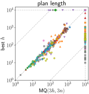
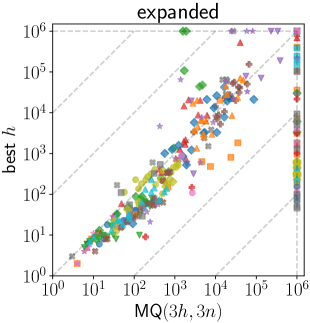
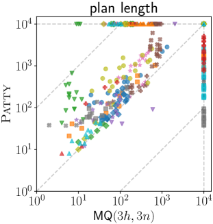
Figure 2: Left and center: $\text{best }h$, the best SQ GBFS planner for each problem, vs $\text{M}(3h\!\operatorname*{{\|}}\!3n)$ on sequential plan length and number of expanded nodes. Right: Patty vs $\text{M}(3h\!\operatorname*{{\|}}\!3n)$ on sequential plan length. Points on the top left triangle favour $\text{M}(3h\!\operatorname*{{\|}}\!3n)$ and points on the bottom right favour $\text{best }h$ and Patty on the respective plots.

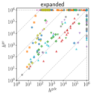
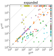
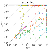
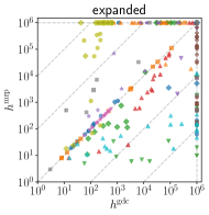
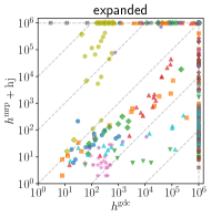
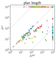
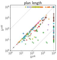
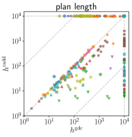
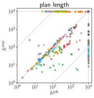
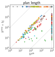
Figure 3: $h^{\text{md}}$ ($x$-axis) vs. various heuristics ($y$-axis) in terms of plan length and number of nodes expanded during search. Top left points benefit $h^{\text{md}}$ and bottom right points the $y$-axis configuration.

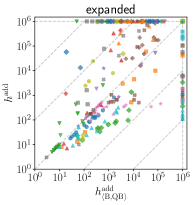
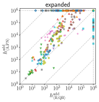
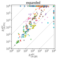
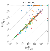
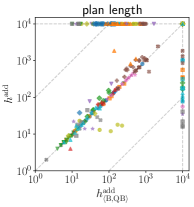
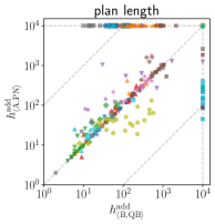
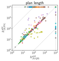
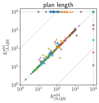
Figure 4: $h^{\text{add}}_{\left<\text{B},\text{QB}\right>}$ ($x$-axis) vs. $h^{\text{add}}$ and other novelty extensions ($y$-axis) in terms of plan length and number of nodes expanded during search. Top left points benefit $h^{\text{add}}_{\left<\text{B},\text{QB}\right>}$ and bottom right points the $y$-axis configuration.

Appendix C Full coverage details

The total coverage of planners over each domain is shown in Table 4. Almost all domains have all problems solved by at least one planner (block-grouping, counters, drone, ext-plant-watering, farmland, fo-counters, fo-farmland, fo-sailing, hydropower, markettrader, pathwaysmetric, sailing, sugar, tpp, and zenotravel). This can either be attributed to small problem sizes, a planner being designed or motivated primarily for the domain, or the problem becomes trivial when not considering plan quality, such as farmland, markettrader or tpp.

The two domains which are difficult for the selected planners are expedition and settlersnumeric. Expedition is a resource transportation problem with the problem that the agent(s) must go back and forth along the transportation path due to having limited fuel and carrying capacity. The considered heuristics cannot reason about the requirement of going back and forth due to being derived from delete relaxation. Settlersnumeric is modelling a civilisation-like game which requires managing resources to build town structures. There is a large number of predicates in this problem and again delete relaxation heuristics cannot detect long range dependencies of resources, e.g. wood is needed to build a saw mill which in turn also needs wood to create timber. The domain is solved well by LP-RPG (Coles et al. 2013) whose paper introduced and was motivated by the domain.

	SQ GBFS						MQ GBFS			PF GBFS			SMT
domain	$h^{\text{md}}$	$h^{\text{add}}$	$h^{\text{mrp}}\text{{+hj}}$	$h^{\text{md}}_{\left<\text{B},\text{QB}\right>}$	$h^{\text{add}}_{\left<\text{B},\text{QB}\right>}$	$h^{\text{mrp}}_{\left<\text{B},\text{QB}\right>}\text{{+hj}}$	$\text{M}({3h})$	$\text{M}(3n)$	$\text{M}(3h\!\operatorname*{{\|}}\!3n)$	$\text{P}(3h)$	$\text{P}(3n)$	$\text{P}(3h\!\operatorname*{{\|}}\!3n)$	Patty	best
block-grouping	15	16	19	15	15	19	16	12	15	18	16	17	20	20
counters	13	13	20	10	10	20	14	9	11	20	19	20	20	20
delivery	17	14	10	14	11	10	19	10	17	18	12	16	5	19
drone	20	11	17	5	15	17	16	18	17	19	16	19	4	20
expedition	3	2	-	3	6	-	3	5	8	3	6	6	3	8
ext-plant-watering	12	12	20	1	19	20	17	20	20	20	20	20	6	20
farmland	20	20	20	20	20	20	20	20	20	20	20	20	20	20
fo-counters	9	7	-	15	12	-	9	14	14	8	14	10	20	20
fo-farmland	20	5	13	20	20	14	20	20	20	20	20	20	20	20
fo-sailing	-	4	-	-	1	-	3	-	-	3	1	4	20	20
hydropower	3	2	-	18	20	-	3	20	20	2	20	20	20	20
markettrader	17	4	-	20	20	-	15	20	20	17	20	19	-	20
mprime	7	16	16	12	18	16	19	18	17	17	18	18	14	19
pathwaysmetric	-	2	12	-	2	13	3	2	3	12	13	12	20	20
rover	10	4	7	12	5	7	13	12	16	11	12	12	16	16
sailing	-	18	20	-	17	20	20	19	20	20	20	20	20	20
settlersnumeric	-	2	3	-	-	4	4	-	2	4	3	5	-	5
sugar	1	9	16	-	8	18	12	9	9	18	18	19	20	20
tpp	20	3	4	5	4	4	17	4	7	20	4	20	3	20
zenotravel	13	19	20	15	13	20	18	12	18	20	20	18	11	20
sum	200	183	217	185	236	222	261	244	274	290	292	315	262	367

Table 4: Coverage of various configurations of single queue (S), multi-queue (M), and portfolio (P) GBFS, and the Patty solver on the NT-IPC domains. The rightmost column records the highest coverage for each domain. The top scores for each row except the rightmost column are indicated by the cell colour intensity with the top score being highlighted in bold.

References

- Arxer and Scala (2023) Arxer, J. E.; and Scala, E. 2023. International Planning Competition 2023 - Numeric Tracks. https://ipc2023-numeric.github.io. Accessed: 2024-02-19.
- Bofill, Espasa, and Villaret (2017) Bofill, M.; Espasa, J.; and Villaret, M. 2017. Relaxed Exists-Step Plans in Planning as SMT. In IJCAI, 563–570.
- Cardellini, Giunchiglia, and Maratea (2024) Cardellini, M.; Giunchiglia, E.; and Maratea, M. 2024. Symbolic Numeric Planning with Patterns. In AAAI, 20070–20077.
- Coles et al. (2008) Coles, A.; Fox, M.; Long, D.; and Smith, A. 2008. A Hybrid Relaxed Planning Graph-LP Heuristic for Numeric Planning Domains. In ICAPS, 52–59.
- Coles et al. (2013) Coles, A. J.; Coles, A.; Fox, M.; and Long, D. 2013. A Hybrid LP-RPG Heuristic for Modelling Numeric Resource Flows in Planning. J. Artif. Intell. Res., 46: 343–412.
- Corrêa and Seipp (2022) Corrêa, A. B.; and Seipp, J. 2022. Best-First Width Search for Lifted Classical Planning. In ICAPS, 11–15.
- Fawcett et al. (2011) Fawcett, C.; Helmert, M.; Hoos, H.; Karpas, E.; Röger, G.; and Seipp, J. 2011. FD-Autotune: Domain-Specific Configuration using Fast Downward. In ICAPS 2011 Workshop on Planning and Learning.
- Fox and Long (2003) Fox, M.; and Long, D. 2003. PDDL2.1: An Extension to PDDL for Expressing Temporal Planning Domains. J. Artif. Intell. Res., 20: 61–124.
- Garrett, Kaelbling, and Lozano-Pérez (2016) Garrett, C. R.; Kaelbling, L. P.; and Lozano-Pérez, T. 2016. Learning to Rank for Synthesizing Planning Heuristics. In IJCAI, 3089–3095.
- Gigante and Scala (2023) Gigante, N.; and Scala, E. 2023. On the Compilability of Bounded Numeric Planning. In IJCAI, 5341–5349.
- Helmert (2002) Helmert, M. 2002. Decidability and Undecidability Results for Planning with Numerical State Variables. In AIPS, 44–53.
- Helmert (2006) Helmert, M. 2006. The Fast Downward Planning System. J. Artif. Intell. Res., 191–246.
- Helmert, Röger, and Karpas (2011) Helmert, M.; Röger, G.; and Karpas, E. 2011. Fast Downward Stone Soup: A Baseline for Building Planner Portfolios. In ICAPS 2011 Workshop on Planning and Learning.
- Hoffmann (2002) Hoffmann, J. 2002. Extending FF to Numerical State Variables. In ECAI, 571–575.
- Hoffmann (2003) Hoffmann, J. 2003. The Metric-FF Planning System: Translating ”Ignoring Delete Lists” to Numeric State Variables. J. Artif. Intell. Res., 24: 685–758.
- Illanes and McIlraith (2017) Illanes, L.; and McIlraith, S. A. 2017. Numeric Planning via Abstraction and Policy Guided Search. In IJCAI, 4338–4345.
- Katz et al. (2017) Katz, M.; Lipovetzky, N.; Moshkovich, D.; and Tuisov, A. 2017. Adapting Novelty to Classical Planning as Heuristic Search. In ICAPS, 172–180.
- Katz et al. (2018) Katz, M.; Sohrabi, S.; Samulowitz, H.; and Sievers, S. 2018. Delfi: Online planner selection for cost-optimal planning.
- Kuroiwa, Shleyfman, and Beck (2023) Kuroiwa, R.; Shleyfman, A.; and Beck, J. C. 2023. Extracting and Exploiting Bounds of Numeric Variables for Optimal Linear Numeric Planning. In ECAI, 1332–1339.
- Kuroiwa et al. (2021) Kuroiwa, R.; Shleyfman, A.; Piacentini, C.; Castro, M. P.; and Beck, J. C. 2021. LM-cut and Operator Counting Heuristics for Optimal Numeric Planning with Simple Conditions. In ICAPS, 210–218.
- Kuroiwa et al. (2022) Kuroiwa, R.; Shleyfman, A.; Piacentini, C.; Castro, M. P.; and Beck, J. C. 2022. The LM-Cut Heuristic Family for Optimal Numeric Planning with Simple Conditions. J. Artif. Intell. Res., 75: 1477–1548.
- Li et al. (2018) Li, D.; Scala, E.; Haslum, P.; and Bogomolov, S. 2018. Effect-Abstraction Based Relaxation for Linear Numeric Planning. In IJCAI, 4787–4793.
- Lipovetzky and Geffner (2012) Lipovetzky, N.; and Geffner, H. 2012. Width and Serialization of Classical Planning Problems. In ECAI, 540–545.
- Lipovetzky and Geffner (2017) Lipovetzky, N.; and Geffner, H. 2017. Best-First Width Search: Exploration and Exploitation in Classical Planning. In AAAI, 3590–3596.
- Ma et al. (2020) Ma, T.; Ferber, P.; Huo, S.; Chen, J.; and Katz, M. 2020. Online Planner Selection with Graph Neural Networks and Adaptive Scheduling. In AAAI, 5077–5084.
- Piacentini et al. (2018) Piacentini, C.; Castro, M. P.; Ciré, A. A.; and Beck, J. C. 2018. Linear and Integer Programming-Based Heuristics for Cost-Optimal Numeric Planning. In AAAI, 6254–6261.
- Ramírez et al. (2018) Ramírez, M.; Papasimeon, M.; Lipovetzky, N.; Benke, L.; Miller, T.; Pearce, A. R.; Scala, E.; and Zamani, M. 2018. Integrated Hybrid Planning and Programmed Control for Real Time UAV Maneuvering. In AAMAS, 1318–1326.
- Richter and Helmert (2009) Richter, S.; and Helmert, M. 2009. Preferred Operators and Deferred Evaluation in Satisficing Planning. In ICAPS, 273–280.
- Richter and Westphal (2010) Richter, S.; and Westphal, M. 2010. The LAMA Planner: Guiding Cost-Based Anytime Planning with Landmarks. J. Artif. Intell. Res., 39: 127–177.
- Röger and Helmert (2010) Röger, G.; and Helmert, M. 2010. The More, the Merrier: Combining Heuristic Estimators for Satisficing Planning. In ICAPS, 246–249.
- Scala et al. (2017) Scala, E.; Haslum, P.; Magazzeni, D.; and Thiébaux, S. 2017. Landmarks for Numeric Planning Problems. In IJCAI, 4384–4390.
- Scala, Haslum, and Thiébaux (2016) Scala, E.; Haslum, P.; and Thiébaux, S. 2016. Heuristics for Numeric Planning via Subgoaling. In IJCAI, 3228–3234.
- Scala et al. (2016a) Scala, E.; Haslum, P.; Thiébaux, S.; and Ramírez, M. 2016a. Interval-Based Relaxation for General Numeric Planning. In ECAI, 655–663.
- Scala et al. (2020a) Scala, E.; Haslum, P.; Thiébaux, S.; and Ramírez, M. 2020a. Subgoaling Techniques for Satisficing and Optimal Numeric Planning. J. Artif. Intell. Res., 68: 691–752.
- Scala et al. (2016b) Scala, E.; Ramírez, M.; Haslum, P.; and Thiébaux, S. 2016b. Numeric Planning with Disjunctive Global Constraints via SMT. In ICAPS, 276–284.
- Scala et al. (2020b) Scala, E.; Saetti, A.; Serina, I.; and Gerevini, A. E. 2020b. Search-Guidance Mechanisms for Numeric Planning Through Subgoaling Relaxation. In ICAPS, 226–234.
- Seipp et al. (2012) Seipp, J.; Braun, M.; Garimort, J.; and Helmert, M. 2012. Learning Portfolios of Automatically Tuned Planners. In ICAPS, 368–372.
- Shleyfman, Kuroiwa, and Beck (2023) Shleyfman, A.; Kuroiwa, R.; and Beck, J. C. 2023. Symmetry Detection and Breaking in Linear Cost-Optimal Numeric Planning. In ICAPS, 393–401.
- Teichteil-Königsbuch, Ramírez, and Lipovetzky (2020) Teichteil-Königsbuch, F.; Ramírez, M.; and Lipovetzky, N. 2020. Boundary Extension Features for Width-Based Planning with Simulators on Continuous-State Domains. In IJCAI, 4183–4189.