Non-concave distributionally robust stochastic control
in a discrete time finite horizon setting

Abstract.

In this article we present a general framework for non-concave distributionally robust stochastic control problems in a discrete time finite horizon setting. Our framework allows to consider a variety of different path-dependent ambiguity sets of probability measures comprising, as a natural example, the ambiguity set defined via Wasserstein-balls around path-dependent reference measures, as well as parametric classes of probability distributions. We establish a dynamic programming principle which allows to derive both optimal control and worst-case measure by solving recursively a sequence of one-step optimization problems.

As a concrete application, we study the robust hedging problem of a financial derivative under an asymmetric (and non-convex) loss function accounting for different preferences of sell- and buy side when it comes to the hedging of financial derivatives. As our entirely data-driven ambiguity set of probability measures, we consider Wasserstein-balls around the empirical measure derived from real financial data. We demonstrate that during adverse scenarios such as a financial crisis, our robust approach outperforms typical model-based hedging strategies such as the classical Delta-hedging strategy as well as the hedging strategy obtained in the non-robust setting with respect to the empirical measure and therefore overcomes the problem of model misspecification in such critical periods.

Keywords: Distributionally robust stochastic control, model uncertainty, dynamic programming, hedging, data-driven optimization

¹NTU Singapore, Division of Mathematical Sciences,
21 Nanyang Link, Singapore 637371.
²National University of Singapore, Department of Mathematics,
21 Lower Kent Ridge Road, 119077.

1. Introduction

Consider an agent executing a sequence of actions based on the observation she makes in her random environment with the goal to maximize her expected payoff at a predetermined future maturity date. The agent may take decisions based on the current and past observations of the environment, as well as based on her past executions. Sequential decision making problems of this type are usually referred to as (non-Markovian) stochastic control problems and have found a wide range of applications including many in physics (e.g., [28], [31], [46], [77]), economics (e.g., [19], [26], [39], [42], [63]), and finance (e.g., [7], [9], [57], [64], [65], [79]), to name but a few.

However, modeling the underlying probability distribution of the environment in stochastic control problems is, in practice, extraordinarily difficult, as the model choice is subject to a high degree of possible model misspecification, typically referred to as Knightian uncertainty ([41]) or simply as model risk. To account for model risk, one approach known as distributionally robust stochastic control or distributionally robust optimization is to consider an ambiguity set of probability measures, instead of of singleton, which represents the candidates for the true but to the agent unknown probability measure ([12], [14], [23], [29], [33], [44], [47], [62]). The agent then chooses a sequence of actions in order to robustly optimize her expected payoff at maturity with respect to the worst-case probability measure among those in the ambiguity set.

A natural approach to define an ambiguity set of probability measures is to first consider one reference probability measure that can be regarded as the best guess or estimate of the stochastic behavior of the environment. Based on this reference probability measure one then considers all probability measures that are in a certain sense close to the reference probability measure, where proximity is typically measured via the distance of parameters in parametric approaches ([25], [35], [72]) or via some distance between probability measures in non-parametric approaches ([5], [32], [56], [73], [75]). In such a setting, the agent is more protected against model misspecification and typically performs well even if her first guess for the true law of the environment, modeled by the reference measure, is not correct, but in some sense close enough.

In this article we analyze a general setting for distributionally robust stochastic control problems in a discrete time finite horizon setting.

In our main result presented in Theorem 3.1 we prove the existence of both an optimal control and a worst-case measure. More precisely, we establish in Theorem 3.1 a dynamic programming principle which allows us to obtain both optimal control and worst-case measure by solving recursively a sequence of one step optimization problems.

Our framework to model distributional uncertainty is formulated in great generality and is not restricted to a specific type of model ambiguity but rather pursues a principled approach by imposing general conditions on ambiguity sets of probability measures, cf. Assumption 2.1. From a technical point of view, we introduce a new stability condition on the ambiguity sets of probability measures (see Assumption 2.1 (iii)) which then, together with an application of Berge’s maximum principle [8], allows to derive the main result described above.

We demonstrate in Section 4 that Assumption 2.1 is naturally fulfilled by important classes of ambiguity sets such as Wasserstein-balls around reference probability measures and by parametric classes of probability distributions. Therefore, we present a unified framework for both parametric and non-parametric (in particular data-driven) approaches to describe distributional uncertainty.

Moreover, in contrast to most literature on (distributionally robust) stochastic optimal control (see, e.g., [3], [4], [6], [10], [11], [13], [16], [24], [27], [34], [37], [43], [45], [50], [52], [53], [55], [59], [60], [76]) our objective function is not required to be concave (nor convex) and hence opens the door to analyze the distributionally robust optimization of important classes of problems that are usually difficult to solve due to the obstacle of non-concavity ([2], [17], [21], [22], [48], [49], [51], [58], [66]).

As a concrete application, we study in Section 5 the robust hedging of a financial derivative under an asymmetric (and non-convex) loss function accounting for different preferences of sell- and buy side when it comes to the hedging of financial derivatives ([15], [18], and [30]). As our entirely data-driven ambiguity set of probability measures, we consider Wasserstein-balls around the empirical measure derived from real financial data. We demonstrate that during adverse scenarios such as a financial crisis, our robust approach outperforms typical model-based hedging strategies such as the classical Delta-hedging strategy as well as the hedging strategy obtained in the non-robust setting with respect to the empirical measure and therefore overcomes the problem of model misspecification in such critical periods. To provide evidence, we test on data from the peak of the financial disruptions during the COVID-19 crisis in March $2020$ which constitutes a recent example for a major adverse distribution change in financial markets.

The remainder of this paper is as follows. In Section 2 we introduce the setting of our distributionally robust stochastic control problem. Section 3 contains our main result: a dynamic programming principle guaranteeing the existence of an optimizer as well as a worst-case probability measure for our distributionally robust stochastic control problem. In Section 4 we present several possible ambiguity sets of probability measures satisfying our assumptions. Section 5 contains a description of our deep learning based numerical routine which we apply to analyze a data-driven hedging problem under asymmetric preferences. The proofs are provided in Section 6.

2. Setting

To formulate our optimization problem, we consider a fixed and finite time horizon $T\in\mathbb{N}$ as well as a closed set ${\Omega_{\operatorname{loc}}}\subseteq\mathbb{R}^{d}$ for $d\in\mathbb{N}$. Then, we introduce the set

$$\Omega^{t}:=\underbrace{{\Omega_{\operatorname{loc}}}\times\cdots\times{\Omega_{\operatorname{loc}}}}_{t-\text{ times }},\qquad t=1\dots,T,$$

and we define a filtration $(\mathcal{F}_{t})_{t=0,\dots,T}$ by setting $\mathcal{F}_{t}:=\mathcal{B}(\Omega^{t})$ for $t=1,\dots,T$ as well as $\mathcal{F}_{0}:=\{\emptyset,\Omega\}$, where we abbreviate

$$(\Omega,\mathcal{F}):=(\Omega^{T},\mathcal{F}_{T}).$$

For every $k\in\mathbb{N}$, $X\subseteq\mathbb{R}^{k}$, and $p\in\mathbb{N}_{0}$, we define the set of continuous functions $g:X\rightarrow\mathbb{R}$ which additionally possess polynomial growth at most of degree $p$ via

$$C_{p}(X,\mathbb{R}):=\left\{g\in C(X,\mathbb{R})~{}\middle|~{}\sup_{x\in X}\frac{|g(x)|}{1+\|x\|^{p}}<\infty\right\},$$

where $C(X,\mathbb{R})$ denotes the set of continuous functions mapping from $X$ to $\mathbb{R}$, and where here and in the following $\|\cdot\|$ always denotes the Euclidean norm on the respective Euclidean space. We define on $C_{p}({\Omega_{\operatorname{loc}}},\mathbb{R})$ the norm

$$\|g\|_{C_{p}}:=\sup_{x\in{\Omega_{\operatorname{loc}}}}\frac{|g(x)|}{1+\|x\|^{p}}.$$

Moreover, for each $t=1,\dots,T$ and $p\in\mathbb{N}_{0}$, we denote by $\mathcal{M}_{1}^{p}(\Omega^{t})$ the set of all probability measures on $(\Omega^{t},\mathcal{B}(\Omega^{t}))$ with finite $p$-th moment. We define an ambiguity set of probability measures by fixing for $t=0$ a set of probability measures $\mathcal{P}_{0}\subseteq\mathcal{M}_{1}^{p}({\Omega_{\operatorname{loc}}})$, whereas for all $t=1,\dots,T-1$ we consider a correspondence

$$\Omega^{t} \rightarrow\left(\mathcal{M}_{1}^{p}({\Omega_{\operatorname{loc}}}),\tau_{p}\right)$$

$$\omega^{t} \twoheadrightarrow\mathcal{P}_{t}(\omega^{t}),$$

where $\tau_{p}$ for some fixed $p\in\mathbb{N}_{0}$ refers to the topology induced by convergence of measures in $\mathcal{M}_{1}^{p}({\Omega_{\operatorname{loc}}})$ with respect to $\|\cdot\|_{C_{p}}$, i.e., we have

(2.1) $$\mu_{n}\xrightarrow{\tau_{p}}\mu\text{ for }n\rightarrow\infty~{}\Leftrightarrow~{}\lim_{n\rightarrow\infty}\int g{\mathop{}\!\mathrm{d}}\mu_{n}=\int g{\mathop{}\!\mathrm{d}}\mu\text{ for all }g\in C_{p}({\Omega_{\operatorname{loc}}},\mathbb{R}).$$

In particular, for $p=0$, the topology $\tau_{0}$ coincides with the topology of weak convergence, whereas for $p\geq 1$, $\tau_{p}$ coincides with the topology induced by the $p$-Wasserstein metric $\operatorname{d}_{W_{p}}(\cdot,\cdot)$. Recall that for $q\in\mathbb{N}$ we have for two probability measures $\mu_{1},\mu_{2}\in\mathcal{M}_{1}^{q}({\Omega_{\operatorname{loc}}})$ with finite $q$-moment that their Wasserstein-distance of order $q$ is defined as

$$\operatorname{d}_{W_{q}}\left(\mu_{1},\mu_{2}\right):=\inf_{\pi\in\Pi(\mu_{1},\mu_{2})}\left(\int_{{\Omega_{\operatorname{loc}}}\times{\Omega_{\operatorname{loc}}}}\|x-y\|^{q}\pi({\mathop{}\!\mathrm{d}}x,{\mathop{}\!\mathrm{d}}y)\right)^{1/q},$$

where $\Pi(\mu_{1},\mu_{2})\subset\mathcal{M}_{1}^{q}({\Omega_{\operatorname{loc}}}\times{\Omega_{\operatorname{loc}}})$ denotes the set of all joint distributions of $\mu_{1}$ and $\mu_{2}$, i.e., the set of all probability measures on ${\Omega_{\operatorname{loc}}}\times{\Omega_{\operatorname{loc}}}$ with first marginal $\mu_{1}$ and second marginal $\mu_{2}$, compare for more details, e.g., [70].

Then, we impose the following assumption on the correspondences $(\mathcal{P}_{t})_{t=0,\dots,T-1}$.

Assumption 2.1.

Fix $p\in\mathbb{N}_{0}$. Then, for every $t\in\{1,\dots,T-1\}$ we assume the following.

• The correspondence $\Omega^{t}\ni\omega^{t}\twoheadrightarrow\mathcal{P}_{t}(\omega^{t})\subseteq\left(\mathcal{M}_{1}^{p}({\Omega_{\operatorname{loc}}}),\tau_{p}\right)$ is compact-valued, continuous, and non-empty. Moreover, if $p=0$, we additionally assume that $\mathcal{P}_{t}(\omega^{t})\subseteq\mathcal{M}_{1}^{1}({\Omega_{\operatorname{loc}}})$ for all $\omega^{t}\in\Omega^{t}$.

• There exists some $C_{P,t}\geq 1$ such that for all $\omega^{t}:=(\omega_{1}^{t},\dots,\omega_{t}^{t})\in\Omega^{t}$ and for all $\mathbb{P}\in\mathcal{P}_{t}\left(\omega^{t}\right)$ we have

  (2.2) $$\int_{{\Omega_{\operatorname{loc}}}}\|x\|^{p}\mathbb{P}({\mathop{}\!\mathrm{d}}x)\leq C_{P,t}\left(1+\sum_{i=1}^{t}\|\omega_{i}^{t}\|^{p}\right).$$

• There exists some $L_{P,t}>0$ such that for all $\omega^{t}:=(\omega_{1}^{t},\dots,\omega_{t}^{t})\in\Omega^{t}$, $\widetilde{\omega}^{t}:=(\widetilde{\omega}_{1}^{t},\dots,\widetilde{\omega}_{t}^{t})\in\Omega^{t}$ and for all $\mathbb{P}\in\mathcal{P}_{t}\left(\omega^{t}\right)$ there exists some $\widetilde{\mathbb{P}}\in\mathcal{P}_{t}\left(\widetilde{\omega}^{t}\right)$ satisfying

  (2.3) $$\operatorname{d}_{W_{1}}(\mathbb{P},\widetilde{\mathbb{P}})\leq L_{P,t}\left(\sum_{i=1}^{t}\|\omega_{i}^{t}-\widetilde{\omega}_{i}^{t}\|\right).$$

• The set $\mathcal{P}_{0}\subseteq\left(\mathcal{M}_{1}^{p}({\Omega_{\operatorname{loc}}}),\tau_{p}\right)$ is non-empty, compact, and there exists $C_{P,0}\geq 1$ such that

  (2.4) $$\int_{{\Omega_{\operatorname{loc}}}}\|x\|^{p}\mathbb{P}({\mathop{}\!\mathrm{d}}x)\leq C_{P,0}$$

  for all $\mathbb{P}\in\mathcal{P}_{0}$.

We can now define a probability measure $\mathbb{P}:=\mathbb{P}_{0}\otimes\dots\otimes\mathbb{P}_{T-1}\in\mathcal{M}_{1}(\Omega)$ by

(2.5) $$\mathbb{P}(B)=\mathbb{P}_{0}\otimes\dots\otimes\mathbb{P}_{T-1}(B):=\int_{{\Omega_{\operatorname{loc}}}}\dots\int_{{\Omega_{\operatorname{loc}}}}1\mathrm{l}_{B}(\omega_{1},\dots,\omega_{T})\mathbb{P}_{T-1}(\omega_{1},\dots,\omega_{T-1};{\mathop{}\!\mathrm{d}}\omega_{T})\dots\mathbb{P}_{0}({\mathop{}\!\mathrm{d}}\omega_{1}),$$

for $B\in\mathcal{F}$. This allows us to define the ambiguity set $\mathfrak{P}\subseteq\mathcal{M}_{1}(\Omega)$ of admissible probability measures on $\Omega$ by

$$\mathfrak{P}:=\bigg{\{}\mathbb{P}_{0}\otimes\dots\otimes\mathbb{P}_{T-1}~{}\bigg{|}~{} \mathbb{P}_{t}(\cdot)\in\mathcal{P}_{t}(\cdot),~{}t=0,\dots,T-1,$$

$$\mathbb{P}_{t}:\Omega^{t}\rightarrow\mathcal{M}_{1}({\Omega_{\operatorname{loc}}})\text{ Borel - measurable}\bigg{\}}.$$

Remark 2.2.

Kuratovskis Theorem (see, e.g., [1, Theorem 18.13]) provides for each $t\in\{1,\dots,T-1\}$ the existence of a measurable kernel $\mathbb{P}_{t}:\Omega^{t}\rightarrow\mathcal{M}_{1}^{p}({\Omega_{\operatorname{loc}}})$ such that $\mathbb{P}_{t}(\omega^{t})\in\mathcal{P}_{t}(\omega^{t})$ for all $\omega^{t}\in\Omega^{t}$.

Next, we consider at each time $t=0,\dots,T-1$ a compact set $A_{t}\subset\mathbb{R}^{m_{t}}$ for some $m_{t}\in\mathbb{N}$, and define the set of $(A_{t})_{t=0,\dots,T-1}$-valued controls by

$$\mathcal{A}:=\bigg{\{}\mathbf{a}=(a_{t})_{t=0,\dots,T-1}~{}\bigg{|}~{} a_{t}:\Omega\rightarrow A_{t},~{}a_{t}\text{ is }\mathcal{F}_{t}\text{-measurable for all }t=0,\dots,T-1\bigg{\}}.$$

To define our optimization problem, we consider a function $\Psi:\Omega\times A^{T}\rightarrow\mathbb{R}$ which fulfils the assumptions below.

Assumption 2.3.

Let $p\in\mathbb{N}_{0}$ be the integer from Assumption 2.1. Then, we assume the map

$$\Omega\times A^{T} \rightarrow\mathbb{R}$$

$$(\omega,a)\mapsto\Psi(\omega,a)$$

satisfies the following:

• There exists some $L_{\Psi}>0$ such that for all $\omega=(\omega_{1},\dots,\omega_{T}),\widetilde{\omega}=(\widetilde{\omega}_{1},\dots,\widetilde{\omega}_{T})\in\Omega$ and for all $a=(a_{0},\dots,a_{T-1}),\widetilde{a}=(\widetilde{a}_{0},\dots,\widetilde{a}_{T-1})\in A^{T}$ we have

  (2.6) $$\left|\Psi\left(\omega,a\right)-\Psi\left(\widetilde{\omega},\widetilde{a}\right)\right|\leq L_{\Psi}\cdot\left(\sum_{i=1}^{T}\left\|\omega_{i}-\widetilde{\omega}_{i}\right\|+\|a_{i-1}-\widetilde{a}_{i-1}\|\right).$$

• There exists some $C_{\Psi}\geq 1$ such that for all $a\in A^{T}$ and for all $\omega=(\omega_{1},\dots,\omega_{T})\in\Omega$ we have

  $$\left|\Psi(\omega,a)\right|\leq C_{\Psi}\cdot\left(1+\sum_{i=1}^{T}\|\omega_{i}\|^{p}\right).$$

This allows to analyze the following distributionally robust stochastic optimal control problem which consists in solving the max-min problem

(2.7) $$\sup_{\mathbf{a}\in\mathcal{A}}\inf_{\mathbb{P}\in\mathfrak{P}}\mathbb{E}_{\mathbb{P}}\left[\Psi(a_{0},\dots,a_{T-1})\right],$$

i.e., our goal is to choose a control that maximizes the expected valued of $\Psi$ under the worst case probability measure.

3. Dynamic Programming Principle and Main Result

Let $t\in\{1,\dots,T-1\}$, let $\omega^{t}\in\Omega^{t}$, ${\omega}_{\operatorname{loc}}\in{\Omega_{\operatorname{loc}}}$ and write $\omega^{t}\otimes_{t}{\omega}_{\operatorname{loc}}:=(\omega^{t},{\omega}_{\operatorname{loc}})\in\Omega^{t+1}$. Then, we set

$$\Psi_{T}:\equiv\Psi,$$

which allows for all $t=T-1,\dots,1$ to define recursively the following quantities:

(3.1) $$\Omega^{t}\times A^{t+1}\ni\left(\omega^{t},a^{t+1}\right)\mapsto J_{t}(\omega^{t},a^{t+1}): =\inf_{\mathbb{P}\in\mathcal{P}_{t}(\omega^{t})}\mathbb{E}_{\mathbb{P}}\left[\Psi_{t+1}\left(\omega^{t}\otimes_{t}\cdot,a^{t+1}\right)\right]$$

$$=\inf_{\mathbb{P}\in\mathcal{P}_{t}(\omega^{t})}\int_{{\Omega_{\operatorname{loc}}}}\Psi_{t+1}\left((\omega^{t},{\omega}_{\operatorname{loc}}),a^{t+1}\right)\mathbb{P}({\mathop{}\!\mathrm{d}}{\omega}_{\operatorname{loc}}),$$

as well as

(3.2) $$\Omega^{t}\times A^{t}\ni\left(\omega^{t},a^{t}\right)\mapsto \Psi_{t}(\omega^{t},a^{t}):=\sup_{\widetilde{a}\in A_{t}}J_{t}\left(\omega^{t},(a^{t},\widetilde{a})\right).$$

Moreover, for $t=0$ we define

(3.3) $$A_{0}\ni a\mapsto J_{0}(a) :=\inf_{\mathbb{P}\in\mathcal{P}_{0}}\mathbb{E}_{\mathbb{P}}\left[\Psi_{1}\left(\cdot,a\right)\right],$$

$$\Psi_{0} :=\sup_{\widetilde{a}\in A_{0}}J_{0}(\widetilde{a}).$$

In the following theorem we formulate our main result that establishes the existence of an optimal control and a worst-case measure for our distributionally robust stochastic optimal control problem (2.7) as well as a dynamic programming principle.

Theorem 3.1.

Suppose Assumption 2.1 and Assumption 2.3 are fulfilled. Then the following holds.

• Let $t\in\{1,\dots,T-1\}$. Then, there exists a measurable selector

  (3.4) $$\Omega^{t}\times A^{t}\ni(\omega^{t},a^{t})\mapsto\widetilde{a}_{t}^{*}\left(\omega^{t},a^{t}\right)\in A_{t}$$

  such that for all $(\omega^{t},a^{t})\in\Omega^{t}\times A^{t}$

  (3.5) $$\Psi_{t}(\omega^{t},a^{t})=J_{t}\left(\omega^{t},\,\left(a^{t},\widetilde{a}_{t}^{*}\left(\omega^{t},a^{t}\right)\right)\,\right).$$

  In addition, there exists $a_{0}^{*}\in A_{0}$ such that

  (3.6) $$\Psi_{0}=J_{0}(a_{0}^{*}).$$

  Moreover, for all $t\in\{1,\dots,T-1\}$ there exists a measurable selector

  (3.7) $$\Omega^{t}\times A^{t+1}\ni(\omega^{t},a^{t+1})\mapsto\widetilde{\mathbb{P}}_{t}^{*}(\omega^{t},a^{t+1})\in\mathcal{P}_{t}(\omega^{t})$$

  such that for all $(\omega^{t},a^{t+1})\in\Omega^{t}\times A^{t+1}$ we have

  (3.8) $$\mathbb{E}_{\widetilde{\mathbb{P}}_{t}^{*}(\omega^{t},a^{t+1})}\left[\Psi_{t+1}\left(\omega^{t}\otimes_{t}\cdot,a^{t+1}\right)\right]=\inf_{\mathbb{P}\in\mathcal{P}_{t}(\omega^{t})}\mathbb{E}_{\mathbb{P}}\left[\Psi_{t+1}\left(\omega^{t}\otimes_{t}\cdot,a^{t+1}\right)\right].$$

  In addition, there exists a measurable selector $A_{0}\ni a\mapsto\widetilde{\mathbb{P}}_{0}^{*}(a)\in\mathcal{P}_{0}$ such that for all $a\in A$ we have

  (3.9) $$\mathbb{E}_{\widetilde{\mathbb{P}}_{0}^{*}(a)}\left[\Psi_{1}\left(\cdot,a\right)\right]=\inf_{\mathbb{P}\in\mathcal{P}_{0}}\mathbb{E}_{\mathbb{P}}\left[\Psi_{1}\left(\cdot,a\right)\right].$$

• For every $t\in\{1,\dots,T-1\}$ let $\widetilde{a}_{t}^{*}$ be the measurable selector from (3.4) and let $a_{0}^{*}$ be defined in (3.6), and define

  $$\Omega^{t}\ni\omega^{t}=(\omega_{1},\dots,\omega_{t})\mapsto a_{t}^{*}(\omega^{t}):=\widetilde{a}_{t}^{*}\left(\omega^{t},~{}\left(a_{0}^{*},\dots,a_{t-1}^{*}(\omega_{1},\dots,\omega_{t-1}\right)\right)\in A_{t}.$$

  Moreover, for every $t\in\{1,\dots,T-1\}$ let $\widetilde{\mathbb{P}}_{t}^{*}$ denote the measurable selector from (3.7) and define

  $$\Omega^{t}\ni\omega^{t}\mapsto{\mathbb{P}}_{t}^{*}(\omega^{t}):=\widetilde{\mathbb{P}}_{t}^{*}(\omega^{t},(a_{s}^{*}(\omega^{s}))_{s=0,\dots,t}))\in\mathcal{P}_{t}(\omega^{t}).$$

  In addition, let $\widetilde{\mathbb{P}}_{0}^{*}$ denote the measurable selector from (3.9) and define $\mathbb{P}_{0}^{*}:=\widetilde{\mathbb{P}}_{0}^{*}(a_{0}^{*})$. Then for ${\mathbf{a}}^{*}:=(a_{t}^{*})_{t=0,\dots,T-1}\in\mathcal{A}$ and $\mathbb{P}^{*}:=\mathbb{P}_{0}^{*}\otimes\cdots\otimes\mathbb{P}_{T-1}^{*}\in\mathfrak{P}$ we have

  (3.10) $$\sup_{a\in\mathcal{A}}\inf_{\mathbb{P}\in\mathfrak{P}}\mathbb{E}_{\mathbb{P}}\left[\Psi(a_{0},\dots,a_{T-1})\right]=\inf_{\mathbb{P}\in\mathfrak{P}}\mathbb{E}_{\mathbb{P}}\left[\Psi(a_{0}^{*},\dots,a_{T-1}^{*})\right]=\mathbb{E}_{\mathbb{P}^{*}}\left[\Psi\left(a_{0}^{*},\dots,a_{T-1}^{*}\right)\right].$$

4. Modeling Ambiguity

In this section we propose two important possible choices to model ambiguity sets and show that our framework supports the use of these ambiguity sets. In Section 4.1 we discuss ambiguity sets that are modeled as Wasserstein-balls around reference measures while in Section 4.2 we present ambiguity sets incorporating parametric uncertainty.

4.1. Modeling ambiguity with the Wasserstein distance

The following result shows that the important canonical example of an ambiguity set given by a $\varepsilon$-Wasserstein-ball with radius $\varepsilon>0$ fulfils the assumption formulated in Assumption 2.1.

Proposition 4.1.

For $t\in\{1,\dots,T-1\}$, $q\in\mathbb{N}$, let $\Omega^{t}\ni\omega^{t}\mapsto\widehat{\mathbb{P}}_{t}(\omega^{t})\in\left(\mathcal{M}_{1}^{q}({\Omega_{\operatorname{loc}}}),\tau_{q}\right)$ be $L_{B}$-Lipschitz continuous for some $L_{B}>0$, i.e., for all $\omega^{t},\widetilde{\omega}^{t}\in\Omega^{t}$ we have $\operatorname{d}_{W_{q}}(\widehat{\mathbb{P}}_{t}(\omega^{t}),\widehat{\mathbb{P}}_{t}(\widetilde{\omega}^{t}))\leq L_{B}\cdot\left(\sum_{i=1}^{t}\|\omega_{i}^{t}-\widetilde{\omega}_{i}^{t}\|\right)$ and let $\varepsilon_{t}>0$. Moreover, consider some $\widehat{\mathbb{P}}_{0}\in\mathcal{M}_{1}^{q}({\Omega_{\operatorname{loc}}})$ and some $\varepsilon_{0}>0$. Furthermore, assume that ${\Omega_{\operatorname{loc}}}$ is convex.

Then, the ambiguity set defined by

$$\Omega^{t}\ni\omega^{t}\mapsto\mathcal{P}_{t}\left({\omega}^{t}\right):=\mathcal{B}_{\varepsilon_{t}}^{(q)}\left(\widehat{\mathbb{P}}_{t}(\omega^{t})\right):=\left\{\mathbb{P}\in\mathcal{M}_{1}^{q}({\Omega_{\operatorname{loc}}})~{}\middle|~{}\operatorname{d}_{W_{q}}\left(\widehat{\mathbb{P}}_{t}(\omega^{t}),~{}\mathbb{P}\right)\leq\varepsilon_{t}\right\} \text{ for }t\in\{1,\dots,T-1\},$$

$$\mathcal{P}_{0}:=\mathcal{B}_{\varepsilon_{0}}^{(q)}\left(\widehat{\mathbb{P}}_{0}\right):=\left\{\mathbb{P}\in\mathcal{M}_{1}^{q}({\Omega_{\operatorname{loc}}})~{}\middle|~{}\operatorname{d}_{W_{q}}\left(\widehat{\mathbb{P}}_{0},~{}\mathbb{P}\right)\leq\varepsilon_{0}\right\} \text{ for }t=0,$$

satisfies Assumption 2.1 if $p<q$.

4.2. Modeling ambiguity in parametric models

In this section we show that the setting from Section 2 also allows to consider parametric families of distributions as ambiguity sets with corresponding ambiguity described by time-dependent parameter sets $(\Theta_{t})_{t=0,\dots,T-1}$.

To this end, for each $t\in\{0,1,\dots,T-1\}$ let $\left(\mathbb{P}_{\theta}\right)_{\theta\in\Theta_{t}}\subseteq\mathcal{M}_{1}({\Omega_{\operatorname{loc}}})$ be a family of probability measures parameterized by $\theta\in\Theta_{t}$, and let $p\in\mathbb{N}_{0}$ be the integer from Assumption 2.1. Then, we impose the following assumptions.

1. For each $t\in\{0,1,\dots,T-1\}$ let $\Theta_{t}\in\mathbb{R}^{D_{t}}$ for some $D_{t}\in\mathbb{N}$ be non-empty, convex, and closed.

2. For each $t\in\{0,1,\dots,T-1\}$ let the map

   $$\mathbb{R}^{D_{t}}\supseteq\Theta_{t} \rightarrow\left(\mathcal{M}_{1}^{\max\{1,p\}}({\Omega_{\operatorname{loc}}}),\tau_{\max\{1,p\}}\right)$$

   $$\theta \mapsto\mathbb{P}_{\theta}({\mathop{}\!\mathrm{d}}x)$$

   be Lipschitz, i.e., there exists some constant $L_{P_{\theta},t}>0$ such that $\operatorname{d}_{W_{\max\{1,p\}}}\left(\mathbb{P}_{\theta_{1}},\mathbb{P}_{\theta_{2}}\right)\leq L_{P_{\theta},t}\cdot\|\theta_{1}-\theta_{2}\|$ for all $\theta_{1},\theta_{2}\in\Theta_{t}$.

3. For each $t\in\{1,\dots,T-1\}$ let the map

   $$\widehat{\theta}_{t}:\Omega^{t} \rightarrow\Theta_{t}\in\mathbb{R}^{D_{t}}$$

   $$\omega^{t}=(\omega_{1}^{t},\dots,\omega_{t}^{t}) \mapsto\widehat{\theta}_{t}(\omega_{1}^{t},\dots,\omega_{t}^{t})$$

   be Lipschitz, i.e., there exists some constant $L_{\theta}>0$ such that $\left\|\widehat{\theta}_{t}(\omega_{1},\dots,\omega_{t})-\widehat{\theta}_{t}(\widetilde{\omega}_{1},\dots,\widetilde{\omega}_{t})\right\|\leq L_{\theta}\cdot\sum_{i=1}^{t}\|\omega_{i}^{t}-\widetilde{\omega}_{i}^{t}\|$ for all $\omega^{t},\widetilde{\omega}^{t}\in\Omega^{t}$.

4. For each $t\in\{1,\dots,T-1\}$ and for any $\varepsilon_{t}>0$ we define

   $$\mathcal{P}_{t}^{(\varepsilon_{t})}(\omega_{1},\dots,\omega_{t}):=\left\{\mathbb{P}_{\theta}({\mathop{}\!\mathrm{d}}x)\in\mathcal{M}_{1}^{\max\{1,p\}}({\Omega_{\operatorname{loc}}})~{}\middle|~{}\theta\in\Theta_{t}\text{ with }\|\theta-\widehat{\theta}_{t}(\omega_{1},\dots,\omega_{t})\|\leq\varepsilon_{t}\right\}.$$

5. For $t=0$ let $\widehat{\theta}_{0}\in\Theta_{0}$, and for any $\varepsilon_{0}>0$ we define

   $$\mathcal{P}_{0}^{(\varepsilon_{0})}:=\left\{\mathbb{P}_{\theta}({\mathop{}\!\mathrm{d}}x)\in\mathcal{M}_{1}^{\max\{1,p\}}({\Omega_{\operatorname{loc}}})~{}\middle|~{}\theta\in\Theta_{0}\text{ with }\|\theta-\widehat{\theta}_{0}\|\leq\varepsilon_{0}\right\}.$$

Proposition 4.2.

For each $t\in\{0,1,\dots,T-1\}$ let $\left(\mathbb{P}_{\theta}\right)_{\theta\in\Theta_{t}}\subseteq\mathcal{M}_{1}({\Omega_{\operatorname{loc}}})$ be a family of probability measures parameterized by $\theta\in\Theta_{t}$, and let $p\in\mathbb{N}_{0}$ be the integer from Assumption 2.1. Moreover, assume that assumptions (A1) - (A5) holds. Then Assumption 2.1 is satisfied.

With the following example we present a parametric family of distributions fulfilling the above mentioned assumptions (A1) - (A5) and therefore also, according to Proposition 4.2, Assumption 2.1.

Proposition 4.3.

Let ${\Omega_{\operatorname{loc}}}=[0,\infty)$ and for each $t\in\{0,1,\dots,T-1\}$ let $\Theta_{t}:=[0,\infty)$. For each $\theta\in\Theta_{t}$ define $\mathbb{P}_{\theta}$ by

$$\mathbb{P}_{\theta}:=\begin{cases}\operatorname{Exp}\left(\tfrac{1}{\theta}\right)&\text{ if }\theta>0,\\ \delta_{\{0\}}&\text{ if }\theta=0,\end{cases}$$

i.e., as an exponential distribution with rate parameter $\tfrac{1}{\theta}$ if $\theta>0$ and as the Dirac measure at $0$ if $\theta=0$. Moreover, we let $\theta_{0}\in\Theta_{0}$ and define for each $t\in\{1,\dots,T-1\}$

(4.1) $$\widehat{\theta}_{t}:\Omega^{t} \rightarrow\Theta_{t}$$

$$(\omega_{1},\dots,\omega_{t}) \mapsto\frac{1}{t}\sum_{i=1}^{t}\omega_{i}.$$

Then, for any $\left(\varepsilon_{t}\right)_{t=0,\dots,t-1}\subseteq(0,\infty)$ and for any $p\in\mathbb{N}_{0}$, the set-valued maps

$$\Omega^{t}\ni\omega^{t}\twoheadrightarrow\mathcal{P}_{t}(\omega^{t}) :=\left\{\mathbb{P}_{\theta}({\mathop{}\!\mathrm{d}}x)\in\mathcal{M}_{1}^{\max\{1,p\}}({\Omega_{\operatorname{loc}}})~{}\middle|~{}\theta\in\Theta_{t}\text{ with }\|\theta-\widehat{\theta}_{t}(\omega^{t})\|\leq\varepsilon_{t}\right\}$$

$$\mathcal{P}_{0} :=\left\{\mathbb{P}_{\theta}({\mathop{}\!\mathrm{d}}x)\in\mathcal{M}_{1}^{\max\{1,p\}}({\Omega_{\operatorname{loc}}})~{}\middle|~{}\theta\in\Theta_{0}\text{ with }\|\theta-\widehat{\theta}_{0}\|\leq\varepsilon_{0}\right\}$$

satisfy (A1) - (A5).

Remark 4.4.

• Note that for each $(\theta_{n})_{n\in\mathbb{N}}\subset(0,\infty)$ with $\lim_{n\rightarrow\infty}\theta_{n}=0$ we have that $\mathbb{P}_{\theta_{n}}\sim\operatorname{Exp}\left(\frac{1}{\theta_{n}}\right)$ converges for any $p\in\mathbb{N}_{0}$ in $\tau_{p}$ to $\delta_{\{0\}}=:\mathbb{P}_{0}$. Indeed, the corresponding characteristic function satisfies

  $$\varphi_{\mathbb{P}_{\theta_{n}}}(t)=\frac{1}{1-it{\theta_{n}}}\rightarrow 1=\varphi_{\delta_{\{0\}}}(t)\text{ for all }t\in\mathbb{R}\text{ as }n\rightarrow\infty,$$

  which by Lévy’s continuity theorem for characteristic functions implies the result for $p=0$. If $p>0$ note that additionally

  $$\int_{0}^{\infty}|x|^{p}\mathbb{P}_{\theta_{n}}({\mathop{}\!\mathrm{d}}x)=\frac{p!}{\left(\tfrac{1}{\theta_{n}}\right)^{p}}=p!\theta_{n}^{p}\rightarrow 0=\int_{0}^{\infty}|x|^{p}\delta_{\{0\}}({\mathop{}\!\mathrm{d}}x)\text{ as }n\rightarrow\infty.$$

  Therefore, the result now follows by [54, Theorem 2.2.1].

• Further, note that $\widehat{\theta}_{t}$ defined in (4.1) corresponds to the maximum likelihood estimator for the parametric family of distributions $\mathbb{P}_{\theta}\sim\operatorname{Exp}\left(\tfrac{1}{\theta}\right),~{}\theta\in(0,\infty)$. Indeed, for any $\theta\in(0,\infty)$, let $\Omega^{t}\ni(\omega_{1},\dots,\omega_{t})\mapsto L(\omega_{1},\dots,\omega_{t}|\theta):=\prod_{i=1}^{t}\frac{1}{\theta}e^{-\frac{1}{\theta}\omega_{i}}$ denote the likelihood function and

  $$\Omega^{t}\ni(\omega_{1},\dots,\omega_{t})\mapsto\ell(\omega_{1},\dots,\omega_{t}|\theta):=\log\left(L(\omega_{1},\dots,\omega_{t}|\theta)\right)=t\cdot\log\left(\tfrac{1}{\theta}\right)-\frac{1}{\theta}\sum_{i=1}^{t}\omega_{i}$$

  the log-likelihood function. Then, the partial derivative of the log-likelihood function w.r.t. $\theta$ is given by

  $$\frac{\partial}{\partial\theta}\ell(\omega_{1},\dots,\omega_{t}|\theta)=-\frac{t}{\theta}+\frac{1}{\theta^{2}}\sum_{i=1}^{t}\omega_{i}$$

  which vanishes, since $\theta>0$ by assumption, if and only if $\theta=\frac{1}{t}\sum_{i=1}^{t}\omega_{i}$.

5. Applications

5.1. Numerics

To solve our optimization problem (2.7) numerically, we apply the dynamic programming principle from Theorem 3.1. The numerical routine which is summarized in Algorithm 1 approximates optimal actions $(a_{t}^{*})_{t=0,\dots,T-1}$ as defined in Theorem 3.1 by means of deep neural networks.

Input : Hyperparameters for the neural networks; Number of iterations $\operatorname{Iter}_{\Psi}$ for the improvement of each function $\Psi_{t}$; Number of iterations $\operatorname{Iter}_{a}$ for the improvement of the action function; Number of measures $N_{\mathcal{P}}$; Number of Monte-Carlo simulations $N_{\operatorname{MC}}$; State space ${\Omega_{\operatorname{loc}}}$; Action spaces $(A_{t})_{t=0,\dots,T-1}$; Payoff function $\Psi$;

Set ${\mathcal{NN}_{\Psi,T}}\equiv\Psi$;

for $t=T-1,\dots,0$ do

       Initialize a neural network ${\mathcal{NN}_{\Psi,t}}:(\mathbb{R}^{d})^{t}\times(\mathbb{R}^{m_{0}}\times\cdots\mathbb{R}^{m_{t-1}})\rightarrow\mathbb{R}$;

       Initialize a neural network ${\mathcal{NN}_{a,t}}:(\mathbb{R}^{d})^{t}\times(\mathbb{R}^{m_{0}}\times\cdots\mathbb{R}^{m_{t-1}})\rightarrow A_{t}$;

      

      for $\operatorname{iteration}=1,\dots,\operatorname{Iter}_{a}$ do

             Sample $(\omega_{1},\dots,\omega_{t})=\omega^{t}\in\Omega^{t}$;

            

            Sample $(a_{0},\dots,a_{t-1})=a^{t}\in A^{t}$;

             for $k=1,\dots,N_{\mathcal{P}}$ do

                   Sample next states $w^{t+1,(k),(i)}\sim\mathbb{P}_{k}\in\mathcal{P}_{t}(\omega^{t})$ for $i=1,\dots,N_{MC}$

             end for

            Maximize

$$\min_{k}\frac{1}{N_{MC}}\sum_{i=1}^{N_{MC}}{\mathcal{NN}_{\Psi,t+1}}\left((\omega^{t},w^{t+1,(k),(i)}),~{}\left(a^{t},{\mathcal{NN}_{a,t}}(\omega^{t},a^{t})\right)\right)$$

w.r.t. the parameters of the neural network $\mathcal{NN}_{a,t}$;

       end for

      

      for $\operatorname{iteration}=1,\dots,\operatorname{Iter}_{\Psi}$ do

             Sample $(\omega_{1},\dots,\omega_{t})=\omega^{t}\in\Omega^{t}$;

            

            Sample $(a_{0},\dots,a_{t-1})=a^{t}\in A^{t}$;

             for $k=1,\dots,N_{\mathcal{P}}$ do

                   Sample next states $w^{t+1,(k),(i)}\sim\mathbb{P}_{k}\in\mathcal{P}_{t}(\omega^{t})$ for $i=1,\dots,N_{MC}$

             end for

            Minimize

$$\left({\mathcal{NN}_{\Psi,t}}(\omega^{t},a^{t})-\min_{k}\frac{1}{N_{MC}}\sum_{i=1}^{N_{MC}}{\mathcal{NN}_{\Psi,t+1}}\left((\omega^{t},w^{t+1,(k),(i)}),~{}\left(a^{t},{\mathcal{NN}_{a,t}}(\omega^{t},a^{t})\right)\right)\right)^{2}$$

w.r.t. the parameters of the neural network ${\mathcal{NN}_{\Psi,t}}$;

       end for

      

end for

Define $a_{0}:={\mathcal{NN}_{a}^{0}}$; for $t=1,\dots,T-1$ do

       Define $\Omega^{t}\ni\omega^{t}=(\omega_{1},\dots,\omega_{t})\mapsto a_{t}(\omega^{t}):={\mathcal{NN}_{a,t}}\left(\omega^{t},~{}\left(a_{0},\dots,a_{t-1}(\omega_{1},\dots,\omega_{t-1}\right)\right)\in A_{t};$

end for

Output : Actions $(a_{t})_{t=0,\dots,T-1}$;

Algorithm 1 Training of optimal actions

5.2. Data-driven hedging with asymmetric loss functions

We consider some underlying financial asset attaining values $S_{0},S_{1},\dots,S_{T}$ over the future time horizon $0,1,\dots,T$ as well as some financial derivative with payoff $\Phi(S_{0},\dots,S_{T})$ paid at maturity $T$. We face the problem of having sold the derivative at initial time $0$ and therefore being exposed to possibly unexpected high payoff obligations $\Phi(S_{0},\dots,S_{T})$. To reduce this risk, we are interested in hedging the payoff obligation $\Phi(S_{0},\dots,S_{T})$ by investing in the underlying asset such that our potential exposure is reduced, compare also, e.g. [36] for further financial background on hedging of financial derivatives.

We start by modeling an ambiguity set of probability measures and follow to this end the approach outlined in Section 4.1. The underlying asset returns in the time period between $t-1$ and $t$ are given by

$$\mathcal{R}_{t}:=\frac{S_{t}-S_{t-1}}{S_{t-1}}\in{\Omega_{\operatorname{loc}}}\subseteq\mathbb{R},\qquad t\in\{1,\dots,T\},$$

where ${\Omega_{\operatorname{loc}}}=[-C,C]\subset\mathbb{R}$ for some constant value $C>0$. To construct ambiguity sets of probability measures, we consider a time series of historical realized returns

(5.1) $$\left(\mathscr{R}_{1},\dots,\mathscr{R}_{N}\right)\in{\Omega_{\operatorname{loc}}}^{N},\qquad\text{ for some }N\in\mathbb{N}.$$

Relying on the time series from (5.1), we design ambiguity sets $\mathcal{P}_{t}$, $t=0,\dots,T-1$. To this end, we define $\widehat{\mathbb{P}}_{0}$ through a sum of Dirac-measures given by

(5.2) $$\widehat{\mathbb{P}}_{0}({\mathop{}\!\mathrm{d}}x):=\frac{1}{N}\sum_{s=1}^{N}\delta_{\mathscr{R}_{s}}({\mathop{}\!\mathrm{d}}x)\in\mathcal{M}_{1}({\Omega_{\operatorname{loc}}}),$$

and $\widehat{\mathbb{P}}_{t}$ for $t=1,\dots,T-1$ by

(5.3) $$\Omega^{t}\ni\omega^{t}=(\omega_{1},\dots,\omega_{t})\mapsto\widehat{\mathbb{P}}_{t}\left(\omega^{t}\right)({\mathop{}\!\mathrm{d}}x):=\sum_{s=t}^{N-1}\pi_{s}^{t}(\omega^{t})\cdot\delta_{\mathscr{R}_{s+1}}({\mathop{}\!\mathrm{d}}x)\in\mathcal{M}_{1}({\Omega_{\operatorname{loc}}}),$$

where $\pi_{s}^{t}(\omega^{t})\in[0,1]$, $s=t,\cdots,N-1$ with $\sum_{s=t}^{N-1}\pi_{s}^{t}(\omega^{t})=1$. We want to weight the distance between the past $t$ returns before $\mathcal{R}_{t+1}$ and the $t$ returns before $\mathscr{R}_{s+1}$, while assigning higher probabilities to more similar sequences of $t$ returns. This means, the measure $\widehat{\mathbb{P}}_{t}$ relies its probabilities for the realization of the next return on the best fitting sequence of $t$ consecutive returns that precede the prediction. To this end, we set

$$\Omega^{t}\ni\omega^{t}\mapsto\pi_{s}^{t}(\omega^{t}):=\left(\frac{\exp(-\beta\operatorname{dist}_{s}(\omega^{t})^{2})}{\sum_{\ell=t}^{N-1}\exp(-\beta\operatorname{dist}_{\ell}(\omega^{t})^{2})}\right),$$

for $\beta>0$ and with

$$\operatorname{dist}_{s}(\omega^{t}):=\left\|\left(\mathscr{R}_{s-t+1},\cdots,\mathscr{R}_{s}\right)-\omega^{t}\right\|=\left\|\left(\mathscr{R}_{s-t+1},\cdots,\mathscr{R}_{s}\right)-\left(\omega_{1},\cdots,\omega_{t}\right)\right\|,~{}~{}$$

for all $s=t,\cdots,N-1$. Then, for any $\left(\varepsilon_{t}\right)_{t=0,\dots,t-1}\subseteq(0,\infty)$ we define ambiguity sets of probability measures via

(5.4) $$\Omega^{t}\ni\omega^{t}\mapsto\mathcal{P}_{t}\left({\omega}^{t}\right):=\mathcal{B}_{\varepsilon_{t}}^{(1)}\left(\widehat{\mathbb{P}}_{t}(\omega^{t})\right) \text{ for }t\in\{1,\dots,T-1\},$$

$$\mathcal{P}_{0}:=\mathcal{B}_{\varepsilon_{0}}^{(1)}\left(\widehat{\mathbb{P}}_{0}\right) \text{ for }t=0,$$

where $\mathcal{B}_{\varepsilon}^{(1)}\left(\widehat{\mathbb{P}}\right)$ denotes a Wasserstein-ball of order $1$ with radius $\varepsilon$ around some probability measure $\widehat{\mathbb{P}}$, as defined in Proposition 4.1.

As our assumptions on the objective function $\Psi$ formulated in Assumption 2.3 do not require the objective function to be concave, we are able to consider non-concave objective function as they appear in behavorial economics and, in particular, in prospect theory ([38]). To this end, we consider a loss function of the form

(5.5) $$\mathbb{R}\ni x\mapsto U(x):=x^{a}1\mathrm{l}_{\{x\geq 0\}}+b\cdot(-x)^{a}1\mathrm{l}_{\{x<0\}}\qquad\text{ where }a\in(0,1),b>1,$$

which assigns the value $x^{a}$ to positive inputes $x$ and $bx^{a}$ to negative inputs $x$, see also [67] or [74], and compare the illustration in Figure 1 (a). Considering an asymmetric loss function as in (5.5) accounts for the empirical fact that agents exhibit distinct behaviors in response to gains and losses, namely they are much more sensitive with respect to losses. Experimental studies reported in [68] provide estimates of $a=0.88$, $b=2.25$.

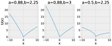
(a) $U(x)$

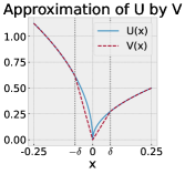
(b) $V(x)$

Figure 1. (a) The three plots show the loss function described in (5.6) for different choices of the parameters $a$ and $b$.
(b) The plot shows an approximation of $U$ with $a=0.5$, $b=2.25$ by the function $V$ described in (5.6) with $\delta=0.075$

Note that $U$ is not Lipschitz-continuous at $0$, hence to meet the requirements from Assumption 2.3, we modify the function $U$ slightly by defining for some fixed small $\delta>0$

(5.6) $$\mathbb{R}\ni x\mapsto V(x):=\begin{cases}U(x)&\text{ if }|x|>\delta,\\ -x\cdot\frac{U(-\delta)}{\delta}&\text{ if }x\in[-\delta,0],\\ x\cdot\frac{U(\delta)}{\delta}&\text{ if }x\in(0,\delta],\end{cases}$$

i.e., we simply interpolate linearly between $U(-\delta)$, $0$, and $U(\delta)$, compare also Figure 1 (b). Note that, by construction, $V$ is Lipschitz-continuous. To define our optimization problem, we consider some financial derivative with payoff function $\Phi(S_{0},S_{1},\dots,S_{T})$. The agent’s goal is to find a hedging strategy, i.e., a combination of an initial cash position $d_{0}$ and time-dependent positions $(\Delta_{i})_{i=0,\dots,T-1}$ invested in the underlying asset minimizing the hedging error between the time-$T$ value of the self-financing hedging strategy given by

$$d_{0}+\sum_{j=0}^{T-1}\Delta_{j}(S_{j+1}-S_{j})=d_{0}+\sum_{j=0}^{T-1}\Delta_{j}\left\{S_{0}\left(\prod_{k=1}^{j}(\omega_{k}+1)\right)\cdot\omega_{j+1}\right\}$$

and the payoff of $\Phi$. To this end, we identify the financial positions of the agent with her actions and define for some $\overline{B}>0$ and $\overline{A}>0$ the sets of actions $(A_{T})_{t=0,\dots,T-1}$ by

$$A_{0} :=\left\{(d_{0},\Delta_{0})\in[-\overline{B},\overline{B}]\times[-\overline{A},\overline{A}]\right\},$$

$$A_{t} :=\left\{\Delta_{t}\in[-\overline{A},\overline{A}]\right\},~{}\text{ for }~{}t=1,\dots,T-1,$$

and further introduce the objective function

(5.7) $$\Omega\times A^{T}\ni(\omega,a)\mapsto\Psi(\omega,a):=-V\Bigg{(}d_{0}+\sum_{j=0}^{T-1} \Delta_{j}(S_{j+1}-S_{j})-\Phi(S_{1},\dots,S_{T})\Bigg{)},$$

where we abbreviate $a=\left((d_{0},\Delta_{0}),d_{1},\dots,d_{T-1}\right)\in A^{T}$.

Solving $\sup_{\mathbf{a}\in\mathcal{A}}\inf_{\mathbb{P}\in\mathfrak{P}}\mathbb{E}_{\mathbb{P}}\left[\Psi(a_{0},\dots,a_{T-1})\right]$ with $\Psi$ as defined in (5.7) corresponds to minimizing the distributionally robust expected hedging error induced by $V$ between the outcome of a self-financing hedging strategy and some financial derivative. Considering the situation of a financial institution which has sold the derivative $\Phi$, the asymmetry of $V$ accounts for the fact that a hedging-strategy that leads to higher payoffs than the derivative is considered a better outcome than a hedging-strategy that leads to smaller payoffs than the derivative payoff and therefore to unexpected losses. We refer to [15], [18], and [30] for related literature on asymmetric hedging, but without model uncertainty.

Proposition 5.1.

Assume the framework from Section 5.2 and let $p=0$. Then, the ambiguity sets of probability measures, defined in (5.4), satisfy Assumption 2.1. Moreover, if the payoff function of the derivative $\Phi:\mathbb{R}^{T+1}\rightarrow\mathbb{R}$ is Lipschitz-continuous, then $\Psi$, defined in (5.7), satisfies Assumption 2.3.

To test our approach empirically, we consider a time-series of daily returns of the stock of Apple between beginning of January $2010$ and beginning of Feburary $2020$ to construct data-driven ambiguity sets of probability measures, as described in (5.3) and (5.4), which we use to train our agent. To evaluate the trained strategy, we consider two test periods ranging from beginning of Feburary $2020$ until end of May $2020$, and between beginning of May $2020$ and end of August $2020$, respectively, compare also Figure 2.

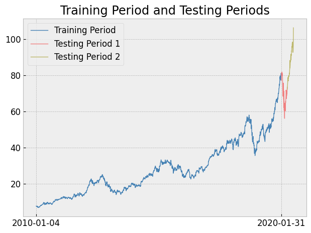
Figure 2. The graph depicts the evolution of the price of the stock of Apple and the separation of the data into a training period (beginning of January $2010$ until beginning of Feburary $2020$) and the two test periods: beginning of Feburary $2020$ until end of May $2020$, and beginning of May $2020$ until end of August $2020$.

We set $T=5$ and we train both a non-robust ($\varepsilon=0$) and a robust hedging strategy with respect to $\varepsilon=0.001$ according to Algorithm 1 for an at-the-money call option with payoff function $\Phi(S_{0},S_{1},\cdots,S_{5})=(S_{5}-S_{0})^{+}$, where we normalize $S_{0}$ to $1$.

To evaluate the performance of our strategy we evaluate on testing period 1 and testing period 2 and show the results in Figure 3 and Tables 1, 2.

The results show that during test period 1 (the advent of the Covid-19 pandemic), the robust hedging strategy outperforms both the non-robust strategy and the classical Black–Scholes delta hedging strategy while in test period 2 the Black–Scholes delta hedging strategy is the best performing strategy. This accounts for the fact that in turbulent times, where the underlying empirical distributions of the asset returns might change dramatically compared to the training period, it turns out to be favourable to take model uncertainty into account as both the non-robust model and the Black–Scholes model rely on misspecified probability distributions. However, in good weather periods (as in test period 2) it is hard to beat a strategy such as the Black–Scholes delta hedging strategy which, due to the assumption of normal asset returns, works reasonably well if no extreme events occur.

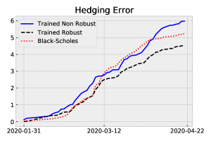
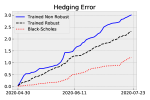
Figure 3. The cumulated hedging errors of the different hedging strategies in the test period 1 (left) and test period 2 (right).

	Non-Robust	Robust	Black–Scholes
No. of days	57	57	57
mean	0.104865	0.079407	0.091882
std	0.092339	0.076183	0.102653
min	0.000900	0.004800	0.000000
25%	0.031000	0.024500	0.024000
50%	0.079800	0.056700	0.061400
75%	0.154100	0.101000	0.130600
max	0.363800	0.371400	0.600100

Table 1. The summary statistics of the hedging errors in Test Period 1

	Non-Robust	Robust	Black–Scholes
No. of days	59	59	59
mean	0.051024	0.039310	0.020795
std	0.048292	0.025909	0.021392
min	0.001400	0.001700	0.000000
25%	0.018350	0.019050	0.006700
50%	0.036400	0.037400	0.013000
75%	0.069700	0.055700	0.024550
max	0.248600	0.119700	0.100300

Table 2. The summary statistics of the hedging errors in Test Period 2

6. Proofs

6.1. Proofs of Section 3

Before reporting the proof of Theorem 3.1, we establish the following lemma.

Lemma 6.1.

Let $t\in\{1,\dots,T-1\}$ and let $\Omega^{t+1}\times A^{t+1}\ni(\omega^{t+1},a^{t+1})\mapsto\Psi_{t+1}(\omega^{t+1},a^{t+1})$ be defined in (3.2). Assume that there exists some $C_{t+1}\geq 1$ and $L_{t+1}>0$ such that for all $\omega^{t+1},\widetilde{\omega}^{t+1}\in\Omega^{t+1}$ and for all $a^{t+1},\widetilde{a}^{t+1}\in A^{t+1}$ we have

(6.1) $$\left|\Psi_{t+1}(\omega^{t+1},a^{t+1})\right|\leq C_{t+1}\cdot\left(1+\sum_{i=1}^{t+1}\|\omega^{t+1}_{i}\|^{p}\right)\text{ for all }(\omega^{t+1},a^{t+1})\in\Omega^{t+1}\times A^{t+1},$$

as well as

(6.2) $$\left|\Psi_{t+1}\left(\omega^{t+1},a^{t+1}\right)-\Psi_{t+1}\left(\widetilde{\omega}^{t+1},\widetilde{a}^{t+1}\right)\right|\leq L_{t+1}\cdot\left(\sum_{i=1}^{t+1}\left\|\omega^{t+1}_{i}-\widetilde{\omega}^{t+1}_{i}\right\|+\|a^{t+1}_{i-1}-\widetilde{a}^{t+1}_{i-1}\|\right).$$

Then, the following holds.

• There exists a measurable map $\Omega^{t}\times A^{t+1}\ni(\omega^{t},a^{t+1})\mapsto\widetilde{\mathbb{P}}_{t}^{*}(\omega^{t},a^{t+1})\in\mathcal{M}_{1}({\Omega_{\operatorname{loc}}})$ satisfying for all $(\omega^{t},a^{t+1})\in\Omega^{t}\times A^{t+1}$ that $\widetilde{\mathbb{P}}_{t}^{*}(\omega^{t},a^{t+1})\in\mathcal{P}_{t}(\omega^{t})$ and

  $$\mathbb{E}_{\widetilde{\mathbb{P}}_{t}^{*}(\omega^{t},a^{t+1})}\left[\Psi_{t+1}\left(\omega^{t}\otimes_{t}\cdot,a^{t+1}\right)\right]=\inf_{\mathbb{P}\in\mathcal{P}_{t}(\omega^{t})}\mathbb{E}_{\mathbb{P}}\left[\Psi_{t+1}\left(\omega^{t}\otimes_{t}\cdot,a^{t+1}\right)\right].$$

• There exists a measurable map $\Omega^{t}\times A^{t}\ni(\omega^{t},a^{t})\mapsto\widetilde{a}_{t}^{*}\left(\omega^{t},a^{t}\right)\in A_{t}$ satisfying for all $(\omega^{t},a^{t})\in\Omega^{t}\times A^{t}$ that

  $$\sup_{\widetilde{a}\in A_{t}}\inf_{\mathbb{P}\in\mathcal{P}_{t}(\omega^{t})}\mathbb{E}_{\mathbb{P}}\left[\Psi_{t+1}\left(\omega^{t}\otimes_{t}\cdot,(a^{t},\widetilde{a})\right)\right]=\inf_{\mathbb{P}\in\mathcal{P}_{t}(\omega^{t})}\mathbb{E}_{\mathbb{P}}\bigg{[}\Psi_{t+1}\bigg{(}\omega^{t}\otimes_{t}\cdot,~{}\left(a^{t},\widetilde{a}_{t}^{*}\left(\omega^{t},a^{t}\right)\right)\bigg{)}\bigg{]}.$$

• There exists some $C_{t}\geq 1$, and some $L_{t}>0$ such that for all $\omega^{t},\widetilde{\omega}^{t}\in\Omega^{t},$ and for all $a^{t},\widetilde{a}^{t}\in A^{t}$ the following inequalities hold

  (6.3) $$\left|\Psi_{t}(\omega^{t},a^{t})\right|\leq C_{t}\cdot\left(1+\sum_{i=1}^{t}\|\omega^{t}_{i}\|^{p}\right),$$

  (6.4) $$\left|\Psi_{t}\left(\omega^{t},a^{t}\right)-\Psi_{t}\left(\widetilde{\omega}^{t},\widetilde{a}^{t}\right)\right|\leq L_{t}\cdot\left(\sum_{i=1}^{t}\left\|\omega^{t}_{i}-\widetilde{\omega}^{t}_{i}\right\|+\|a^{t}_{i-1}-\widetilde{a}^{t}_{i-1}\|\right).$$

Proof of Lemma 6.1.

Let $t\in\{1,\dots,T-1\}$.

We first show the continuity of $\Omega^{t}\times A^{t}\ni(\omega^{t},a^{t})\mapsto\Psi_{t}(\omega^{t},a^{t})$. To that end, we consider the map

$$F:\left\{(\omega^{t},a^{t},a,\mathbb{P})~{}\middle|~{}\omega^{t}\in\Omega^{t},a^{t}\in A^{t},a\in A_{t},\mathbb{P}\in\mathcal{P}_{t}(\omega^{t})\right\} \rightarrow\mathbb{R}$$

$$(\omega^{t},a^{t},a,\mathbb{P}) \mapsto\mathbb{E}_{\mathbb{P}}\left[\Psi_{t+1}\left(\omega^{t}\otimes_{t}\cdot,(a^{t},a)\right)\right]$$

We aim at applying Berge’s maximum theorem (see, e.g., [8] or [1, Theorem 18.19]) to $F$, and therefore first want to show that $F$ is continuous.

We consider a sequence $(\omega^{t}_{n},a^{t}_{n},a_{n},\mathbb{P}_{n})_{n\in\mathbb{N}}\subseteq\left\{(\omega^{t},a^{t},a,\mathbb{P})~{}\middle|~{}\omega^{t}\in\Omega^{t},a^{t}\in A^{t},a\in A_{t},\mathbb{P}\in\mathcal{P}_{t}(\omega^{t})\right\}$ with $(\omega^{t}_{n},a^{t}_{n},a_{n},\mathbb{P}_{n})\rightarrow(\omega^{t},a^{t},a,\mathbb{P})$ as $n\rightarrow\infty$ for some $\omega^{t}\in\Omega^{t}$, $a^{t}\in A^{t}$, $a\in A_{t}$ and $\mathbb{P}\in\mathcal{M}_{1}(\Omega^{t})$. Moreover, we have

$$\left|F\left(\omega^{t}_{n},a^{t}_{n},a_{n},\mathbb{P}_{n}\right)-F\left(\omega^{t},a^{t},a,\mathbb{P}\right)\right|$$

$$\leq\left|F\left(\omega^{t}_{n},a^{t}_{n},a_{n},\mathbb{P}_{n}\right)-F\left(\omega^{t},a^{t},a,\mathbb{P}_{n}\right)\right|+\left|F\left(\omega^{t},a^{t},a,\mathbb{P}_{n}\right)-F\left(\omega^{t},a^{t},a,\mathbb{P}\right)\right|.$$

Note that with $\mathbb{P}_{n}\rightarrow\mathbb{P}$ in $\tau_{p}$ we obtain that $\lim_{n\rightarrow\infty}\left|F\left(\omega^{t},a^{t},a,\mathbb{P}_{n}\right)-F\left(\omega^{t},a^{t},a,\mathbb{P}\right)\right|=0$ as $\Psi_{t+1}$ is by assumption continuous and of polynomial growth of order $p$. Further, we use (6.2) and compute

$$\lim_{n\rightarrow\infty}\left|F\left(\omega^{t}_{n},a^{t}_{n},a_{n},\mathbb{P}_{n}\right)-F\left(\omega^{t},a^{t},a,\mathbb{P}_{n}\right)\right|$$

$$\leq\lim_{n\rightarrow\infty}\int_{{\Omega_{\operatorname{loc}}}}\left|\Psi_{t+1}\left((\omega^{t}_{n},\omega),(a^{t}_{n},a_{n})\right)-\Psi_{t+1}\left((\omega^{t},\omega),(a^{t},a)\right)\right|\mathbb{P}_{n}({\mathop{}\!\mathrm{d}}\omega)$$

$$\leq\lim_{n\rightarrow\infty}\int_{{\Omega_{\operatorname{loc}}}}L_{t+1}\cdot\left(\sum_{i=1}^{t}\bigg{[}\|(\omega^{t}_{n})_{i}-(\omega^{t})_{i}\|+\|(a^{t}_{n})_{i}-(a^{t})_{i}\|+\|a_{n}-a\|\bigg{]}\right)\mathbb{P}_{n}({\mathop{}\!\mathrm{d}}\omega)$$

$$=L_{t+1}\int_{{\Omega_{\operatorname{loc}}}}1\cdot\mathbb{P}({\mathop{}\!\mathrm{d}}\omega)\cdot\lim_{n\rightarrow\infty}\left(\sum_{i=1}^{t}\bigg{[}\|(\omega^{t}_{n})_{i}-(\omega^{t})_{i}\|+\|(a^{t}_{n})_{i}-(a^{t})_{i}\|+\|a_{n}-a\|\bigg{]}\right)=0.$$

We have thus shown that $F$ is continuous. Therefore, by using Assumption 2.1 (i), we may now apply Berge’s maximum theorem which yields that

(6.5) $$\Omega^{t}\times A^{t}\times A_{t}\ni(\omega^{t},a^{t},a)\mapsto\inf_{\mathbb{P}\in\mathcal{P}_{t}(\omega^{t})}\mathbb{E}_{\mathbb{P}}\left[\Psi_{t+1}\left(\omega^{t}\otimes_{t}\cdot,(a^{t},a)\right)\right]$$

is continuous. Note that the above application of Berge’s maximum theorem also implies the existence of a minimizer of (6.5). With the measurable maximum theorem (see, e.g., [1, Theorem 18.19]) we therefore obtain a measurable map $\Omega^{t}\times A^{t+1}\ni(\omega^{t},a^{t+1})\mapsto\widetilde{\mathbb{P}}_{t}^{*}(\omega^{t},a^{t+1})\in\mathcal{P}_{t}(\omega^{t})$ satisfying for all $(\omega^{t},a^{t+1})\in\Omega^{t}\times A^{t+1}$ that

$$\mathbb{E}_{\widetilde{\mathbb{P}}_{t}^{*}(\omega^{t},a^{t+1})}\left[\Psi_{t+1}\left(\omega^{t}\otimes_{t}\cdot,a^{t+1}\right)\right]=\inf_{\mathbb{P}\in\mathcal{P}_{t}(\omega^{t})}\mathbb{E}_{\mathbb{P}}\left[\Psi_{t+1}\left(\omega^{t}\otimes_{t}\cdot,a^{t+1}\right)\right],$$

showing (i).

Since $A_{t}$ is compact, we obtain by a repeated application of Berge’s maximum theorem also that

(6.6) $${\Omega_{\operatorname{loc}}}\times A^{t}\ni(\omega^{t},a^{t})\mapsto\sup_{a\in A_{t}}\inf_{\mathbb{P}\in\mathcal{P}_{t}(\omega^{t})}\mathbb{E}_{\mathbb{P}}\left[\Psi_{t+1}\left(\omega^{t}\otimes_{t}\cdot,(a^{t},a)\right)\right]=\Psi_{t}(\omega,a^{t})$$

is continuous and that the maximizer exists. By the measurable maximum theorem we deduce therefore the existence of a measurable map $\Omega^{t}\times A^{t}\ni(\omega^{t},a^{t})\mapsto\widetilde{a}_{t}^{*}\left(\omega^{t},a^{t}\right)\in A_{t}$ satisfying for all $(\omega^{t},a^{t})\in\Omega^{t}\times A^{t}$ that

$$\sup_{\widetilde{a}\in A_{t}}\inf_{\mathbb{P}\in\mathcal{P}_{t}(\omega^{t})}\mathbb{E}_{\mathbb{P}}\left[\Psi_{t+1}\left(\omega^{t}\otimes_{t}\cdot,(a^{t},\widetilde{a})\right)\right]=\inf_{\mathbb{P}\in\mathcal{P}_{t}(\omega^{t})}\mathbb{E}_{\mathbb{P}}\bigg{[}\Psi_{t+1}\bigg{(}\omega^{t}\otimes_{t}\cdot,~{}\left(a^{t},\widetilde{a}_{t}^{*}\left(\omega^{t},a^{t}\right)\right)\bigg{)}\bigg{]},$$

which shows (ii).

It remains to prove (iii). We assume that (6.1) holds and show the polynomial growth condition stated in (6.3). To this end, we consider elements $\omega^{t}\in\Omega^{t}$, $\widetilde{\omega}^{t}\in\Omega^{t}$, $a^{t}\in A^{t}$, $\widetilde{a}^{t}\in A^{t}$, we set $C_{t}:=2C_{t+1}\cdot C_{P,t}\geq 1$ and obtain by (2.2) and (6.1) that

$$\left|\Psi_{t}(\omega^{t},a^{t})\right| \leq\sup_{\widetilde{a}\in A_{t}}\inf_{\mathbb{P}\in\mathcal{P}_{t}(\omega^{t})}\int_{{\Omega_{\operatorname{loc}}}}\left|\Psi_{t+1}\left((\omega^{t},\omega),(a^{t},\widetilde{a})\right)\right|\mathbb{P}({\mathop{}\!\mathrm{d}}\omega)$$

$$\leq\sup_{\widetilde{a}\in A_{t}}\inf_{\mathbb{P}\in\mathcal{P}_{t}(\omega^{t})}\int_{{\Omega_{\operatorname{loc}}}}C_{t+1}\left(1+\sum_{i=1}^{t}\|\omega_{i}^{t}\|^{p}+\|\omega\|^{p}\right)\mathbb{P}({\mathop{}\!\mathrm{d}}\omega)$$

$$=C_{t+1}\left(1+\sum_{i=1}^{t}\|\omega_{i}^{t}\|^{p}+\inf_{\mathbb{P}\in\mathcal{P}_{t}(\omega^{t})}\int_{{\Omega_{\operatorname{loc}}}}\|\omega\|^{p}\mathbb{P}({\mathop{}\!\mathrm{d}}\omega)\right)$$

$$\leq C_{t+1}\left(1+\sum_{i=1}^{t}\|\omega_{i}^{t}\|^{p}+C_{P,t}\left(1+\sum_{i=1}^{t}\|\omega_{i}^{t}\|^{p}\right)\right)$$

$$\leq 2C_{t+1}\cdot C_{P,t}\cdot\left(1+\sum_{i=1}^{t}\|\omega_{i}^{t}\|^{p}\right)=C_{t}\cdot\left(1+\sum_{i=1}^{t}\|\omega_{i}^{t}\|^{p}\right),$$

which indeed proves (6.3). Next, we assume that (6.2) holds and aim at showing (6.4). We first compute

(6.7) $$\Psi_{t}\left(\omega^{t},a^{t}\right)-\Psi_{t}\left(\widetilde{\omega}^{t},\widetilde{a}^{t}\right)$$

$$=\sup_{a\in A_{t}}\inf_{\mathbb{P}\in\mathcal{P}_{t}(\omega^{t})}\mathbb{E}_{\mathbb{P}}\left[\Psi_{t+1}\left(\omega^{t}\otimes_{t}\cdot,(a^{t},a)\right)\right]-\sup_{\widetilde{a}\in A_{t}}\inf_{\widetilde{\mathbb{P}}\in\mathcal{P}_{t}(\widetilde{\omega}^{t})}\mathbb{E}_{\widetilde{\mathbb{P}}}\left[\Psi_{t+1}\left(\widetilde{\omega}^{t}\otimes_{t}\cdot,(\widetilde{a}^{t},\widetilde{a})\right)\right]$$

$$=\inf_{\mathbb{P}\in\mathcal{P}_{t}(\omega^{t})}\mathbb{E}_{\mathbb{P}}\left[\Psi_{t+1}\left(\omega^{t}\otimes_{t}\cdot,(a^{t},{a_{\operatorname{loc}}}^{*})\right)\right]-\sup_{\widetilde{a}\in A_{t}}\inf_{\widetilde{\mathbb{P}}\in\mathcal{P}_{t}(\widetilde{\omega}^{t})}\mathbb{E}_{\widetilde{\mathbb{P}}}\left[\Psi_{t+1}\left(\widetilde{\omega}^{t}\otimes_{t}\cdot,(\widetilde{a}^{t},\widetilde{a})\right)\right]$$

$$\leq\inf_{\mathbb{P}\in\mathcal{P}_{t}(\omega^{t})}\mathbb{E}_{\mathbb{P}}\left[\Psi_{t+1}\left(\omega^{t}\otimes_{t}\cdot,(a^{t},{a_{\operatorname{loc}}}^{*})\right)\right]-\inf_{\widetilde{\mathbb{P}}\in\mathcal{P}_{t}(\widetilde{\omega}^{t})}\mathbb{E}_{\widetilde{\mathbb{P}}}\left[\Psi_{t+1}\left(\widetilde{\omega}^{t}\otimes_{t}\cdot,(\widetilde{a}^{t},{a_{\operatorname{loc}}}^{*}))\right)\right]$$

$$=\inf_{\mathbb{P}\in\mathcal{P}_{t}(\omega^{t})}\left[\Psi_{t+1}\left(\omega^{t}\otimes_{t}\cdot,(a^{t},{a_{\operatorname{loc}}}^{*})\right)\right]-\mathbb{E}_{\mathbb{P}_{1}}\left[\Psi_{t+1}\left(\widetilde{\omega}^{t}\otimes_{t}\cdot,(\widetilde{a}^{t},{a_{\operatorname{loc}}}^{*})\right)\right]$$

$$\leq\mathbb{E}_{\mathbb{P}_{2}}\left[\Psi_{t+1}\left(\omega^{t}\otimes_{t}\cdot,(a^{t},{a_{\operatorname{loc}}}^{*})\right)\right]-\mathbb{E}_{\mathbb{P}_{1}}\left[\Psi_{t+1}\left(\widetilde{\omega}^{t}\otimes_{t}\cdot,(\widetilde{a}^{t},{a_{\operatorname{loc}}}^{*})\right)\right],$$

where ${a_{\operatorname{loc}}}^{*}:=\widetilde{a}_{t}^{*}(\omega^{t},a^{t})\in A_{t}$ with $\widetilde{a}_{t}^{*}$ denoting the minimizer from (ii), where $\mathbb{P}_{1}:=\widetilde{\mathbb{P}}_{t}^{*}(\widetilde{\omega}^{t},{a_{\operatorname{loc}}}^{*})\in\mathcal{P}_{t}(\widetilde{\omega}^{t})$ with $\widetilde{\mathbb{P}}_{t}^{*}$ being the maximizer from (i), and where $\mathbb{P}_{2}\in\mathcal{P}_{t}({\omega}^{t})$ is chosen such that inequality (2.2) in Assumption 2.1 (iii) is fulfilled w.r.t. $\mathbb{P}_{1}$. Then, we denote by $\Pi(\mathbb{P}_{1},\mathbb{P}_{2})\subset\mathcal{P}_{1}({\Omega_{\operatorname{loc}}}\times{\Omega_{\operatorname{loc}}})$ the set of probability measures on ${\Omega_{\operatorname{loc}}}\times{\Omega_{\operatorname{loc}}}$ with respective marginal distributions $\mathbb{P}_{1}$ and $\mathbb{P}_{2}$. We use the representation from (6.7), apply the assumption from (6.2), and have

$$\Psi_{t}\left(\omega^{t},a^{t}\right)-\Psi_{t}\left(\widetilde{\omega}^{t},\widetilde{a}^{t}\right)$$

$$\leq\inf_{\pi\in\Pi(\mathbb{P}_{1},\mathbb{P}_{2})}\int_{{\Omega_{\operatorname{loc}}}\times{\Omega_{\operatorname{loc}}}}\bigg{(}\Psi_{t+1}\left(\omega^{t}\otimes_{t}\omega_{1,\operatorname{loc}},(a^{t},{a_{\operatorname{loc}}}^{*})\right)$$

$$\hskip 85.35826pt-\Psi_{t+1}\left(\widetilde{\omega}^{t}\otimes_{t}\omega_{2,\operatorname{loc}},(\widetilde{a}^{t},{a_{\operatorname{loc}}}^{*})\right)\bigg{)}\pi({\mathop{}\!\mathrm{d}}\omega_{1,\operatorname{loc}},{\mathop{}\!\mathrm{d}}\omega_{2,\operatorname{loc}})$$

$$\leq L_{t+1}\cdot\left(\sum_{i=1}^{t}\left\|\omega^{t}_{i}-\widetilde{\omega}^{t}_{i}\right\|+\|a^{t}_{i-1}-\widetilde{a}^{t}_{i-1}\|\right)$$

$$\hskip 85.35826pt+L_{t+1}\inf_{\pi\in\Pi(\mathbb{P}_{1},\mathbb{P}_{2})}\int_{{\Omega_{\operatorname{loc}}}\times{\Omega_{\operatorname{loc}}}}\|\omega_{1,\operatorname{loc}}-\omega_{2,\operatorname{loc}}\|\pi({\mathop{}\!\mathrm{d}}\omega_{1,\operatorname{loc}},{\mathop{}\!\mathrm{d}}\omega_{2,\operatorname{loc}})$$

$$=L_{t+1}\cdot\left(\sum_{i=1}^{t}\left\|\omega^{t}_{i}-\widetilde{\omega}^{t}_{i}\right\|+\|a^{t}_{i-1}-\widetilde{a}^{t}_{i-1}\|\right)+L_{t+1}\operatorname{d}_{W_{1}}(\mathbb{P}_{1},\mathbb{P}_{2}),$$

where in the last step we applied the definition of the $1$-Wasserstein distance. We now use Assumption 2.1 (iii), set $L_{t}:=2L_{t+1}\max\left\{L_{P,t},1\right\}>0$ and obtain

$$\Psi_{t}\left(\omega^{t},a^{t}\right)-\Psi_{t}\left(\widetilde{\omega}^{t},\widetilde{a}^{t}\right)$$

$$\leq L_{t+1}\cdot\left(\sum_{i=1}^{t}\left\|\omega^{t}_{i}-\widetilde{\omega}^{t}_{i}\right\|+\|a^{t}_{i-1}-\widetilde{a}^{t}_{i-1}\|\right)+L_{t+1}L_{P,t}\left(\sum_{i=1}^{t}\|\omega_{i}^{t}-\widetilde{\omega}_{t}^{t}\|\right)$$

$$\leq L_{t}\cdot\left(\sum_{i=1}^{t}\left\|\omega^{t}_{i}-\widetilde{\omega}^{t}_{i}\right\|+\|a^{t}_{i-1}-\widetilde{a}^{t}_{i-1}\|\right).$$

By interchanging the roles of $\Psi_{t}\left(\omega^{t},a^{t}\right)$ and $\Psi_{t}\left(\widetilde{\omega}^{t},\widetilde{a}^{t}\right)$ we obtain

$$\left|\Psi_{t}\left(\omega^{t},a^{t}\right)-\Psi_{t}\left(\widetilde{\omega}^{t},\widetilde{a}^{t}\right)\right|\leq L_{t}\cdot\left(\sum_{i=1}^{t}\left\|\omega^{t}_{i}-\widetilde{\omega}^{t}_{i}\right\|+\|a^{t}_{i-1}-\widetilde{a}^{t}_{i-1}\|\right).$$

This shows (6.4). ∎

As a consequence of Lemma 6.1 we obtain the following corollary for the case $t=0$.

Corollary 6.2.

Let ${\Omega_{\operatorname{loc}}}\times A_{0}\ni(\omega,a)\mapsto\Psi_{1}(\omega,a)$ be defined in (3.2). Assume that there exists some $C_{1}\geq 1$ and $L_{1}>0$ such that for all $\omega,\widetilde{\omega}\in{\Omega_{\operatorname{loc}}}$ and for all $a,\widetilde{a}\in A_{0}$ we have

(6.8) $$\left|\Psi_{1}(\omega,a)\right|\leq C_{1}\cdot\left(1+\|\omega\|^{p}\right)\text{ for all }(\omega,a)\in{\Omega_{\operatorname{loc}}}\times A_{0},$$

as well as

(6.9) $$\left|\Psi_{1}\left(\omega,a\right)-\Psi_{1}\left(\widetilde{\omega},\widetilde{a}\right)\right|\leq L_{1}\left(||\omega-\widetilde{\omega}\|+\|a-\widetilde{a}\|\right).$$

Then, the following holds.

• There exists a measurable map $A_{0}\ni a\mapsto\widetilde{\mathbb{P}}_{0}^{*}(a)\in\mathcal{M}_{1}({\Omega_{\operatorname{loc}}})$ satisfying for all $a\in A_{0}$ that $\widetilde{\mathbb{P}}_{0}^{*}(a)\in\mathcal{P}_{0}$ and

  $$\mathbb{E}_{\widetilde{\mathbb{P}}_{0}^{*}(a)}\left[\Psi_{1}\left(\cdot,a\right)\right]=\inf_{\mathbb{P}\in\mathcal{P}_{0}}\mathbb{E}_{\mathbb{P}}\left[\Psi_{1}\left(\cdot,a\right)\right].$$

• There exists some $a_{0}^{*}\in A_{0}$ such that

  $$\sup_{\widetilde{a}\in A_{0}}\inf_{\mathbb{P}\in\mathcal{P}_{1}}\mathbb{E}_{\mathbb{P}}\left[\Psi_{1}\left(\cdot,\widetilde{a})\right)\right]=\inf_{\mathbb{P}\in\mathcal{P}_{1}}\mathbb{E}_{\mathbb{P}}\left[\Psi_{1}\left(\cdot,a_{0}^{*})\right)\right].$$

Proof.

This follows by the same arguments as the proof of Lemma 6.1. ∎

Proof of Theorem 3.1.

• Since Assumption 2.3 is fulfilled for $\Psi=\Psi_{T}$, we obtain by a recursive application of Lemma 6.1 (iii) for $t=T-1,\dots,0$ that $\Psi_{t+1}$ satisfies the requirements of Lemma 6.1, i.e., $\Psi_{t+1}$ fulfils (6.1) and (6.2). Then, the assertion follows by Lemma 6.1 (i) and (ii) for $t=T-1,\dots,1$ and by Corollary 6.2 (i) and (ii) for $t=0$.

• Let $t\in\{0,\dots,T-1\}$. In the following, for $\omega^{t}=(\omega_{1},\dots,\omega_{t})\in\Omega^{t}$ we denote for any $0\leq s\leq t$ by $\omega^{s}:=(\omega_{1},\dots,\omega_{s})\in\Omega^{s}$ the first $s$ coordinates of $\omega^{t}$.

  Note that by definition of the kernel $\mathbb{P}_{t}^{*}$ we have for all $\omega^{t}\in\Omega^{t}$ that

  (6.10) $$\inf_{\mathbb{P}\in\mathcal{P}_{t}(\omega^{t})}\mathbb{E}_{\mathbb{P}}\left[\Psi_{t+1}\left(\omega^{t}\otimes_{t}\cdot,~{}(a_{s}^{*}(\omega^{s}))_{s=0,\dots,t}\right)\right]=\mathbb{E}_{\mathbb{P}_{t}^{*}(\omega^{t})}\left[\Psi_{t+1}\left(\omega^{t}\otimes_{t}\cdot,~{}(a_{s}^{*}(\omega^{s}))_{s=0,\dots,t}\right)\right].$$

  Then, by definition of ${\mathbf{a}}^{*}$, $\mathbb{P}_{t}^{*}$ and of $\Psi_{t}$, we obtain for all $\omega^{t}\in\Omega^{t}$ that

  $$\Psi_{t}\left(\omega^{t},(a_{s}^{*}(\omega^{s}))_{s=0,\dots,t-1}\right) =\sup_{\widetilde{a}\in A}J_{t}\left(\omega^{t},~{}((a_{s}^{*}(\omega^{s}))_{s=0,\dots,t-1},\widetilde{a})\right)$$

  $$=J_{t}\left(\omega^{t},~{}((a_{s}^{*}(\omega^{s}))_{s=0,\dots,t-1},a^{*}_{t}(\omega^{t})\right)$$

  $$=\inf_{\mathbb{P}\in\mathcal{P}_{t}(\omega^{t})}\mathbb{E}_{\mathbb{P}}\left[\Psi_{t+1}\left(\omega^{t}\otimes_{t}\cdot,~{}(a_{s}^{*}(\omega^{s}))_{s=0,\dots,t}\right)\right]$$

  $$=\mathbb{E}_{\mathbb{P}_{t}^{*}(\omega^{t})}\left[\Psi_{t+1}\left(\omega^{t}\otimes_{t}\cdot,~{}(a_{s}^{*}(\omega^{s}))_{s=0,\dots,t}\right)\right].$$

  Further, by definition of ${\mathbf{a}}^{*}$, we have for all $\mathbb{P}=\mathbb{P}_{0}\otimes\mathbb{P}_{1}\otimes\cdots\otimes\mathbb{P}_{T-1}\in\mathfrak{P}$ that

  (6.11) $$\mathbb{E}_{\mathbb{P}}\left[\Psi_{t+1}\left(a_{0}^{*},\dots,a_{t}^{*}\right)\right]$$

  $$=\int_{\Omega^{t+1}}\Psi_{t+1}\left((\omega^{t},\omega),~{}(a_{s}^{*}(\omega^{s}))_{s=0,\dots,t}\right)\mathbb{P}_{0}\otimes\cdots\otimes\mathbb{P}_{t}({\mathop{}\!\mathrm{d}}(\omega^{t},\omega))$$

  $$=\int_{\Omega^{t}}\left(\int_{{\Omega_{\operatorname{loc}}}}\Psi_{t+1}\left((\omega^{t},\omega),~{}(a_{s}^{*}(\omega^{s}))_{s=0,\dots,t}\right)\mathbb{P}_{t}(\omega^{t};{\mathop{}\!\mathrm{d}}\omega)\right)\mathbb{P}_{0}\otimes\cdots\otimes\mathbb{P}_{t-1}({\mathop{}\!\mathrm{d}}\omega^{t})$$

  $$\geq\int_{\Omega^{t}}\inf_{\widetilde{\mathbb{P}}_{t}\in\mathcal{P}_{t}(\omega^{t})}\left(\int_{{\Omega_{\operatorname{loc}}}}\Psi_{t+1}\left((\omega^{t},\omega),~{}(a_{s}^{*}(\omega^{s}))_{s=0,\dots,t}\right)\widetilde{\mathbb{P}}_{t}(\omega^{t};{\mathop{}\!\mathrm{d}}\omega)\right)\mathbb{P}_{0}\otimes\cdots\otimes\mathbb{P}_{t-1}({\mathop{}\!\mathrm{d}}\omega^{t})$$

  $$=\int_{\Omega^{t}}\Psi_{t}\left(\omega^{t},~{}(a_{s}^{*}(\omega^{s}))_{s=0,\dots,t-1}\right)\mathbb{P}_{0}\otimes\cdots\otimes\mathbb{P}_{t-1}({\mathop{}\!\mathrm{d}}\omega^{t})$$

  $$=\mathbb{E}_{\mathbb{P}}\left[\Psi_{t}\left(a_{0}^{*},\dots,a_{t-1}^{*}\right)\right].$$

  Repeatedly applied, the above inequality (6.11) yields

  (6.12) $$\mathbb{E}_{\mathbb{P}}\left[\Psi_{T}\left(a_{0}^{*},\dots,a_{T-1}^{*}\right)\right]\geq\Psi_{0},$$

  and since $\mathbb{P}\in\mathfrak{P}$ was chosen arbitrarily we also get, by using $\Psi=\Psi_{T}$, that

  (6.13) $$\inf_{\mathbb{P}\in\mathfrak{P}}\mathbb{E}_{\mathbb{P}}\left[\Psi\left(a_{0}^{*},\dots,a_{T-1}^{*}\right)\right]=\inf_{\mathbb{P}\in\mathfrak{P}}\mathbb{E}_{\mathbb{P}}\left[\Psi_{T}\left(a_{0}^{*},\dots,a_{T-1}^{*}\right)\right]\geq\Psi_{0}.$$

  By considering the measure

  $$\mathbb{P}^{*}:=\mathbb{P}_{0}^{*}\otimes\cdots\otimes\mathbb{P}_{T-1}^{*}\in\mathfrak{P},$$

  and by using (6.10), we obtain equality in (6.11) and (6.12). This means, together with (6.13), that we have

  (6.14) $$\inf_{\mathbb{P}\in\mathfrak{P}}\mathbb{E}_{\mathbb{P}}\left[\Psi\left(a_{0}^{*},\dots,a_{T-1}^{*}\right)\right]\geq\Psi_{0}=\mathbb{E}_{\mathbb{P}^{*}}\left[\Psi\left(a_{0}^{*},\dots,a_{T-1}^{*}\right)\right].$$

  Now let $(a_{s}(\cdot))_{s=0,\dots,T-1}\in\mathcal{A}$ be an arbitrary control. Then, we have for all $\omega^{t}\in\Omega^{t}$ that

  (6.15) $$\mathbb{E}_{\widetilde{\mathbb{P}}_{t}^{*}(\omega^{t},(a_{s}(\omega^{s}))_{s=0,\dots,t})}\left[\Psi_{t+1}\left(\omega^{t}\otimes_{t}\cdot,(a_{s}(\omega^{s}))_{s=0,\dots,t}\right)\right]$$

  $$=\inf_{\mathbb{P}_{t}\in\mathcal{P}_{t}(\omega^{t})}\mathbb{E}_{\mathbb{P}_{t}}\left[\Psi_{t+1}\left(\omega^{t}\otimes_{t}\cdot,(a_{s}(\omega^{s}))_{s=0,\dots,t}\right)\right]$$

  $$\leq\sup_{\widetilde{a}\in A_{t}}\inf_{\mathbb{P}_{t}\in\mathcal{P}_{t}(\omega^{t})}\mathbb{E}_{\mathbb{P}_{t}}\left[\Psi_{t+1}\left(\omega^{t}\otimes_{t}\cdot,\left((a_{s}(\omega^{s}))_{s=0,\dots,t-1},\widetilde{a}\right)\right)\right]$$

  $$=\sup_{\widetilde{a}\in A_{t}}J_{t}\left(\omega^{t},\left((a_{s}(\omega^{s}))_{s=0,\dots,t-1},\widetilde{a}\right)\right)$$

  $$=\Psi_{t}\left(\omega^{t},\left((a_{s}(\omega^{s}))_{s=0,\dots,t-1}\right)\right).$$

  Let $\mathbb{P}=\mathbb{P}_{0}\otimes\cdots\otimes\mathbb{P}_{T-1}\in\mathfrak{P}$ be arbitrary and define

  $$\Omega^{t}\ni\omega^{t}\mapsto{\mathbb{P}}_{t}^{*,a}(\omega^{t}):=\widetilde{\mathbb{P}}_{t}^{*}\left(\omega^{t},~{}(a_{s}(\omega^{s}))_{s=0,\dots,t}\right)\in\mathcal{M}_{1}({\Omega_{\operatorname{loc}}}).$$

  Then (6.15) implies

  (6.16) $$\mathbb{E}_{\mathbb{P}}\left[\Psi_{t}(a_{0},\dots,a_{t-1})\right] =\mathbb{E}_{\mathbb{P}_{0}\otimes\cdots\otimes\mathbb{P}_{t-1}}\left[\Psi_{t}(a_{0},\dots,a_{t-1})\right]$$

  $$\geq\mathbb{E}_{\mathbb{P}_{0}\otimes\mathbb{P}_{1}\otimes\cdots\otimes\mathbb{P}_{t-1}\otimes{\mathbb{P}}_{t}^{*,a}}\left[\Psi_{t+1}(a_{0},\dots,a_{t})\right]$$

  $$\geq\inf_{\mathbb{P}^{\prime}\in\mathfrak{P}}\mathbb{E}_{\mathbb{P}^{\prime}}\left[\Psi_{t+1}(a_{0},\dots,a_{t})\right].$$

  Hence, as $\mathbb{P}\in\mathfrak{P}$ was arbitrary, we obtain from (6.16) that

  (6.17) $$\inf_{\mathbb{P}\in\mathfrak{P}}\mathbb{E}_{\mathbb{P}}\left[\Psi_{t+1}(a_{0},\dots,a_{t})\right]\leq\inf_{\mathbb{P}\in\mathfrak{P}}\mathbb{E}_{\mathbb{P}}\left[\Psi_{t}(a_{0},\dots,a_{t-1})\right].$$

  By a repeated application of the latter inequality (6.17) one sees that

  (6.18) $$\inf_{\mathbb{P}\in\mathfrak{P}}\mathbb{E}_{\mathbb{P}}\left[\Psi(a_{0},\dots,a_{T-1})\right]=\inf_{\mathbb{P}\in\mathfrak{P}}\mathbb{E}_{\mathbb{P}}\left[\Psi_{T}(a_{0},\dots,a_{T-1})\right]\leq\Psi_{0}.$$

  Since $(a_{0},\dots,a_{T-1})\in\mathcal{A}$ was also chosen arbitrarily we obtain that

  (6.19) $$\sup_{a\in\mathcal{A}}\inf_{\mathbb{P}\in\mathfrak{P}}\mathbb{E}_{\mathbb{P}}\left[\Psi(a_{0},\dots,a_{T-1})\right]\leq\Psi_{0},$$

  which implies together with (6.14) that

  $$\sup_{a\in\mathcal{A}}\inf_{\mathbb{P}\in\mathfrak{P}}\mathbb{E}_{\mathbb{P}}\left[\Psi(a_{0},\dots,a_{T-1})\right]=\inf_{\mathbb{P}\in\mathfrak{P}}\mathbb{E}_{\mathbb{P}}\left[\Psi\left(a_{0}^{*},\dots,a_{T-1}^{*}\right)\right]=\Psi_{0}=\mathbb{E}_{\mathbb{P}^{*}}\left[\Psi\left(a_{0}^{*},\dots,a_{T-1}^{*}\right)\right].$$

∎

6.2. Proofs of Section 4

Before reporting the proofs of Proposition 4.1 and 4.2, we establish four auxiliary results. To this end, in the following we use the notation $\Pi(\mu,\nu)\subset\mathcal{M}_{1}(X\times X)$ to describe the set of all joint distributions of probability measures $\mu,\nu\in\mathcal{M}_{1}(X)$ on some space $X$.

Lemma 6.3.

Let $p\in\mathbb{N}_{0}$ and let $\left(X,\|\cdot\|_{X}\right)$ be a separable Banach space. Let $\left(\mu_{1}^{(n)},\mu_{2}^{(n)}\right)_{n\in\mathbb{N}}\subseteq\mathcal{M}_{1}^{p}(X)\times\mathcal{M}_{1}^{p}(X)$ converging in $\tau_{p}\times\tau_{p}$ to some $(\mu_{1}^{\infty},\mu_{2}^{\infty})\in\mathcal{M}_{1}^{p}(X)\times\mathcal{M}_{1}^{p}(X)$. Then $\bigcup_{n\in\mathbb{N}}\Pi(\mu_{1}^{(n)},\mu_{2}^{(n)})$ is relatively compact w.r.t. $\tau_{p}\times\tau_{p}$.

Proof.

For the case $p=0$, this result follows from, e.g., the proof of [20, Lemma 5.2]. Hence, w.l.o.g. we can assume $p>0$. By [20, Proof of Lemma 5.2] we further know that $\bigcup_{n\in\mathbb{N}}\Pi(\mu_{1}^{(n)},\mu_{2}^{(n)})$ is weakly relatively compact. Let $\|\cdot\|_{X\times X}$ be the norm on $X\times X$ defined by

$$\|(x,y)\|_{X\times X}:=\|x\|_{X}+\|y\|_{X},\qquad(x,y)\in X\times X.$$

Then, we have for all $x,y\in X$ that

$$\|(x,y)\|_{X\times X}^{p}=\|(x,0)+(0,y)\|_{X\times X}^{p}\leq 2^{p}\left(\|(x,0)\|_{X\times X}^{p}+\|(0,y)\|_{X\times X}^{p}\right)=2^{p}\left(\|x\|_{X}^{p}+\|y\|_{X}^{p}\right),$$

as well as $\|(x,y)\|_{X\times X}\geq\max\{\|x\|_{X},\|y\|_{X}\}$. Hence, we have for all $R>0$

(6.20) $$\sup_{\pi\in\bigcup_{n\in\mathbb{N}}\Pi(\mu_{1}^{(n)},\mu_{2}^{(n)})}\int_{\{(x,y)\in X\times X:\|(x,y)\|_{X\times X}>R\}}\|(x,y)\|_{X\times X}^{p}\pi({\mathop{}\!\mathrm{d}}x,{\mathop{}\!\mathrm{d}}y)$$

$$\leq 2^{p}\cdot\sup_{\pi\in\bigcup_{n\in\mathbb{N}}\Pi(\mu_{1}^{(n)},\mu_{2}^{(n)})}\int_{\{(x,y)\in X\times X:\|(x,y)\|_{X\times X}>R\}}\|x\|_{X}^{p}\pi({\mathop{}\!\mathrm{d}}x,{\mathop{}\!\mathrm{d}}y)$$

$$\hskip 56.9055pt+2^{p}\cdot\sup_{\pi\in\bigcup_{n\in\mathbb{N}}\Pi(\mu_{1}^{(n)},\mu_{2}^{(n)})}\int_{\{(x,y)\in X\times X:\|(x,y)\|_{X\times X}>R\}}\|y\|_{X}^{p}\pi({\mathop{}\!\mathrm{d}}x,{\mathop{}\!\mathrm{d}}y)$$

$$\leq 2^{p}\cdot\sup_{n\in\mathbb{N}}\int_{\{x\in X:\|x\|_{X}>R\}}\|x\|_{X}^{p}\mu_{1}^{(n)}({\mathop{}\!\mathrm{d}}x)+2^{p}\cdot\sup_{n\in\mathbb{N}}\int_{\{y\in X:\|y\|_{X}>R\}}\|y\|_{X}^{p}\mu_{2}^{(n)}({\mathop{}\!\mathrm{d}}y).$$

Now, the convergence $\lim_{n\rightarrow\infty}\left(\mu_{1}^{(n)},\mu_{2}^{(n)}\right)=(\mu_{1}^{\infty},\mu_{2}^{\infty})$ in $\tau_{p}\times\tau_{p}$ implies with [54, Theorem 2.2.1 (3)] both that

$$\lim_{R\rightarrow\infty}\sup_{n\in\mathbb{N}}\int_{\{x\in X:\|x\|_{X}>R\}}\|x\|_{X}^{p}\mu_{1}^{(n)}({\mathop{}\!\mathrm{d}}x)=0,$$

and that

$$\lim_{R\rightarrow\infty}\sup_{n\in\mathbb{N}}\int_{\{y\in X:\|y\|_{X}>R\}}\|y\|_{X}^{p}\mu_{2}^{(n)}({\mathop{}\!\mathrm{d}}y)=0.$$

Therefore, the integral in (6.20) vanishes as $R\rightarrow\infty$, and the relative compactness of $\bigcup_{n\in\mathbb{N}}\Pi(\mu_{1}^{(n)},\mu_{2}^{(n)})$ in $\tau_{p}\times\tau_{p}$ follows directly by [54, Proposition 2.2.3]. ∎

Lemma 6.4.

Let $X$ be a separable Banach space, and let $p\in\mathbb{N}_{0}$ and $q\in\mathbb{N}$ with $q\geq p$. Moreover, let $f\in C_{q}(X,\mathbb{R})$ be non-negative. Then

$$\mathcal{M}_{1}^{q}(X) \rightarrow\mathbb{R}$$

$$\mu \mapsto\int_{X}f(x)\mu({\mathop{}\!\mathrm{d}}x)$$

is lower semicontinuous w.r.t. $\tau_{p}$.

Proof.

If $p=q$, then the map is continuous by definition of $\tau_{p}=\tau_{q}$. Hence, w.l.o.g. we can assume $q>p$. We define for each $k\in\mathbb{N}$ the function

$$X\ni x\mapsto f_{k}(x):=f(x)\wedge\frac{k\cdot f(x)}{1+\|x\|^{q-p}}.$$

One sees directly that $f_{k}\geq 0$ and that $f_{k}\in C_{p}(X,\mathbb{R})$ for all $k\in\mathbb{N}$. Moreover, we have $f_{k}\uparrow f$ monotonically as $k\rightarrow\infty$. Now, let $(\mu^{(n)})_{n\in\mathbb{N}}\subseteq\mathcal{M}_{1}^{q}(X)$ and $\mu\in\mathcal{M}_{1}^{q}(X)$ such that $\mu^{(n)}\rightarrow\mu$ in $\tau_{p}$. Then, we have by the monotone convergence theorem, since $f_{k}\in C_{p}(X,\mathbb{R})$, and since $f_{k}\leq f$ that

$$\int_{X}f(x)\mu({\mathop{}\!\mathrm{d}}x) =\lim_{k\rightarrow\infty}\int_{X}f_{k}(x)\mu({\mathop{}\!\mathrm{d}}x)$$

$$=\lim_{k\rightarrow\infty}\lim_{n\rightarrow\infty}\int_{X}f_{k}(x)\mu^{(n)}({\mathop{}\!\mathrm{d}}x)$$

$$\leq\lim_{k\rightarrow\infty}\lim_{n\rightarrow\infty}\int_{X}f(x)\mu^{(n)}({\mathop{}\!\mathrm{d}}x)$$

$$=\liminf_{n\rightarrow\infty}\int_{X}f(x)\mu^{(n)}({\mathop{}\!\mathrm{d}}x).$$

∎

Lemma 6.5.

Let $\left(X,\|\cdot\|_{X}\right)$ be a separable Banach space, and let $p\in\mathbb{N}_{0}$ and $q\in\mathbb{N}$ with $q\geq p$. Then, the map

$$\mathcal{M}_{1}^{q}(X)\times\mathcal{M}_{1}^{q}(X) \rightarrow[0,\infty)$$

$$(\mu_{1},\mu_{2}) \mapsto d_{W_{q}}(\mu_{1},\mu_{2})$$

is lower semicontinuous in $\tau_{p}\times\tau_{p}$.

Proof.

The case $p=0$ follows from [20, Corollary 5.3]. Hence, w.l.o.g. we may assume $p\geq 1$. Let $(\mu_{1}^{\infty},\mu_{2}^{\infty})\in\mathcal{M}_{1}^{q}(X)\times\mathcal{M}_{1}^{q}(X)$, and let $(\mu_{1}^{(n)},\mu_{2}^{(n)})_{n\in\mathbb{N}}\subseteq\mathcal{M}_{1}^{q}(X)\times\mathcal{M}_{1}^{q}(X)$ be a sequence with $\lim_{n\rightarrow\infty}(\mu_{1}^{(n)},\mu_{2}^{(n)})=(\mu_{1}^{\infty},\mu_{2}^{\infty})$ in $\tau_{p}\times\tau_{p}$. To prove the lower semicontinuity we need to show that

(6.21) $$\liminf_{n\rightarrow\infty}d_{W_{q}}(\mu_{1}^{(n)},\mu_{2}^{(n)})\geq d_{W_{q}}(\mu_{1}^{\infty},\mu_{2}^{\infty}).$$

Let $(\mu_{1}^{(n_{k})},\mu_{2}^{(n_{k})})_{k\in\mathbb{N}}$ be a subsequence such that

(6.22) $$\lim_{k\rightarrow\infty}d_{W_{q}}(\mu_{1}^{(n_{k})},\mu_{2}^{(n_{k})})=\liminf_{n\rightarrow\infty}d_{W_{q}}(\mu_{1}^{(n)},\mu_{2}^{(n)}).$$

For all $k\in\mathbb{N}$ let $\pi^{(n_{k})}\in\Pi\left(\mu_{1}^{(n_{k})},\mu_{2}^{(n_{k})}\right)$ denote the optimal coupling w.r.t. $d_{W_{q}}$, i.e.,

(6.23) $$\left(\int_{X\times X}\|x-y\|_{X}^{q}\pi^{(n_{k})}({\mathop{}\!\mathrm{d}}x,{\mathop{}\!\mathrm{d}}y)\right)^{1/q}=\inf_{\pi\in\Pi\left(\mu_{1}^{(n)},\mu_{2}^{(n)}\right)}\left(\int_{X\times X}\|x-y\|_{X}^{q}\pi({\mathop{}\!\mathrm{d}}x,{\mathop{}\!\mathrm{d}}y)\right)^{1/q}.$$

Since $\left(\pi^{(n_{k})}\right)_{k\in\mathbb{N}}\subseteq\bigcup_{k\in\mathbb{N}}\Pi\left(\mu_{1}^{(n_{k})},\mu_{2}^{(n_{k})}\right)$, we have by Lemma 6.3 that $\left(\pi^{(n_{k})}\right)_{k\in\mathbb{N}}$ is relatively compact w.r.t. $\tau_{p}\times\tau_{p}$.

Let $\pi^{\infty}\in\mathcal{M}_{1}^{p}(X\times X)$ be a limit point of some subsequence $(\pi^{({n_{k}}_{j})})_{j\in\mathbb{N}}$ w.r.t. $\tau_{p}\times\tau_{p}$. Let $\operatorname{proj}_{i}:X\times X\rightarrow X$ denote the projection on the $i$-th component for $i=1,2$. Since $\pi^{({n_{k}}_{j})}\in\Pi\left(\mu_{1}^{({n_{k}}_{j})},\mu_{2}^{({n_{k}}_{j})}\right)$ for all $j\in\mathbb{N}$ and since $\mu_{i}^{({n_{k}}_{j})}\rightarrow\mu_{i}^{\infty}$ in $\tau_{p}$ for $i=1,2$ as $j\rightarrow\infty$, we have by the continuous mapping theorem that

$$\mu_{i}^{\infty}=\lim_{j\rightarrow\infty}\mu_{i}^{({n_{k}}_{j})}=\lim_{j\rightarrow\infty}\pi^{({n_{k}}_{j})}\circ\operatorname{proj}_{i}^{-1}=\pi^{\infty}\circ\operatorname{proj}_{i}^{-1},$$

where the limits are w.r.t. weak convergence. This means that $\pi^{\infty}\in\Pi\left(\mu_{1}^{\infty},\mu_{2}^{\infty}\right)\subseteq\mathcal{M}_{1}^{q}(X\times X)$. Hence, it follows

$$d_{W_{q}}(\mu_{1}^{\infty},\mu_{2}^{\infty}) \leq\left(\int_{X\times X}\|x-y\|_{X}^{q}\pi^{\infty}({\mathop{}\!\mathrm{d}}x,{\mathop{}\!\mathrm{d}}y)\right)^{1/q}$$

(6.24) $$\leq\liminf_{j\rightarrow\infty}\left(\int_{X\times X}\|x-y\|_{X}^{q}\pi^{({n_{k}}_{j})}({\mathop{}\!\mathrm{d}}x,{\mathop{}\!\mathrm{d}}y)\right)^{1/q}$$

(6.25) $$=\liminf_{j\rightarrow\infty}d_{W_{q}}\left(\mu_{1}^{({n_{k}}_{j})},\mu_{2}^{({n_{k}}_{j})}\right)$$

(6.26) $$=\liminf_{n\rightarrow\infty}d_{W_{q}}\left(\mu_{1}^{(n)},\mu_{2}^{(n)}\right).$$

Indeed, (6.24) follows by Lemma 6.4, (6.25) follows with (6.23), and (6.26) follows from (6.22). ∎

Lemma 6.6.

Let $p\in\mathbb{N}_{0}$ and $q\in\mathbb{N}$ such that $q>p$. Moreover, let $\left(X,\|\cdot\|_{X}\right)$ be a separable Banach space. Then, for any $\widehat{\mu}\in\mathcal{M}_{1}^{q}(X)$ and $\varepsilon>0$, the set

$$\mathcal{B}_{\varepsilon}^{(q)}\left(\widehat{\mu}\right):=\left\{\mu\in\mathcal{M}_{1}^{q}(X)~{}\middle|~{}d_{W_{q}}\left(\mu,\widehat{\mu}\right)\leq\varepsilon\right\}$$

is compact w.r.t. $\tau_{p}$.

Proof.

The case $p=0$ follows, e.g., from [78, Theorem 1]. Hence, w.l.o.g. we can assume $p>0$. First, to see that the set is relatively compact w.r.t. $\tau_{p}$, note that by [78, Lemma 1] we have

$$\sup_{\mu\in\mathcal{B}_{\varepsilon}^{(q)}(\widehat{\mu})}\int_{X}\|x\|_{X}^{p}\|x\|_{X}^{q-p}\mu({\mathop{}\!\mathrm{d}}x)=\sup_{\mu\in\mathcal{B}_{\varepsilon}^{(q)}(\widehat{\mu})}\int_{X}\|x\|_{X}^{q}\mu({\mathop{}\!\mathrm{d}}x)<\infty.$$

Hence, since $[0,\infty)\ni x\mapsto x^{q-p}$ is monotonically divergent as $q>p$, we get relative compactness w.r.t. $\tau_{p}$ from, e.g., [54, Proposition 2.2.3].

To see that $\mathcal{B}_{\varepsilon}^{(q)}\left(\widehat{\mu}\right)$ is closed, we apply Lemma 6.5, and obtain that

(6.27) $$\mathcal{M}_{1}^{q}(X) \rightarrow\mathbb{R}$$

$$\mu \mapsto d_{W_{q}}(\widehat{\mu},\mu)$$

is lower semicontinuous. Hence, $\mathcal{B}_{\varepsilon}^{(q)}\left(\widehat{\mu}\right)$ being a superlevel set of (6.27) is closed. ∎

Proof of Proposition 4.1.

Let $t\in\{0,1,\dots,T\}$ be fixed. We verify that the conditions (i)-(iv) of Assumption 2.1 are fulfilled.

• The ambiguity set $\mathcal{P}_{t}(\omega^{t})$ contains, by definition, for all $\omega^{t}\in\Omega^{t}$ the reference measure $\widehat{\mathbb{P}}_{t}(\omega^{t})$ and is hence non-empty. Moreover, by, e.g., [78, Lemma 1] we have $\mathcal{P}_{t}(\omega^{t})\subseteq\mathcal{M}_{1}^{q}({\Omega_{\operatorname{loc}}})\subseteq\mathcal{M}_{1}^{\max\{1,p\}}({\Omega_{\operatorname{loc}}})$ for all $\omega^{t}\in\Omega^{t}$ as $p<q$.
  The compactness of $\mathcal{P}_{t}(\omega^{t})$ w.r.t. $\tau_{p}$ follows from Lemma 6.6 as $p<q$.
  To show the upper hemicontinuity we mainly follow the lines of the proof of [49, Proposition 3.1]. Therefore, the goal is to apply the characterization of upper hemicontinuity provided in Lemma [1, Theorem 17.20]. Let $({\omega^{t}}^{(n)})_{n\in\mathbb{N}}\subseteq\Omega^{t}$ such that ${\omega^{t}}^{(n)}\rightarrow{\omega^{t}}\in\Omega^{t}$ for $n\rightarrow\infty$. Further, consider a sequence $(\mathbb{P}^{(n)})_{n\in\mathbb{N}}$ such that $\mathbb{P}^{(n)}\in\mathcal{B}^{(q)}_{\varepsilon}\left(\widehat{\mathbb{P}}_{t}({\omega^{t}}^{(n)})\right)=\mathcal{P}_{t}({\omega^{t}}^{(n)})$ for all $n\in\mathbb{N}$, i.e., we have $\left({\omega^{t}}^{(n)},\mathbb{P}^{(n)}\right)_{n\in\mathbb{N}}\subseteq\operatorname{Gr}\mathcal{P}_{t}$, where $\operatorname{Gr}\mathcal{P}_{t}$ denotes the graph of $\mathcal{P}_{t}$.

  Let $(\delta_{n})_{n\in\mathbb{N}}\subseteq(0,1)$ with $\lim_{m\rightarrow\infty}\delta_{n}=0$. Note that, since $\Omega^{t}\ni\omega^{t}\mapsto\widehat{\mathbb{P}}_{t}(\omega^{t})$ is, by assumption, $L_{B}$-Lipschitz continuous we have

  $$\lim_{n\rightarrow\infty}d_{W_{q}}\left(\widehat{\mathbb{P}}_{t}(\omega^{t}),\widehat{\mathbb{P}}_{t}({\omega^{t}}^{(n)})\right)\leq\lim_{n\rightarrow\infty}L_{B}\cdot\|\omega^{t}-{\omega^{t}}^{(n)}\|=0.$$

  Hence, there exists a subsequence $\left(\widehat{\mathbb{P}}_{t}({\omega^{t}}^{(n_{k})})\right)_{k\in\mathbb{N}}$ such that

  (6.28) $$d_{W_{q}}\left(\widehat{\mathbb{P}}_{t}({\omega^{t}}),\widehat{\mathbb{P}}_{t}({\omega^{t}}^{(n_{k})})\right)<\delta_{k}\cdot\varepsilon\text{ for all }k\in\mathbb{N}.$$

  This implies for each $\mathbb{P}^{(n_{k})}$, $k\in\mathbb{N}$, that

  $$d_{W_{q}}\left(\widehat{\mathbb{P}}_{t}({\omega^{t}}),\mathbb{P}^{(n_{k})}\right)\leq d_{W_{q}}\left(\widehat{\mathbb{P}}_{t}({\omega^{t}}),\widehat{\mathbb{P}}_{t}({\omega^{t}}^{(n_{k})})\right)+d_{W_{q}}\left(\widehat{\mathbb{P}}_{t}({\omega^{t}}^{(n_{k})})),\mathbb{P}^{(n_{k})}\right)\leq\delta_{k}\cdot\varepsilon+\varepsilon\leq 2\varepsilon.$$

  Hence, $\mathbb{P}^{(n_{k})}\in\mathcal{B}_{2\varepsilon}^{(q)}(\widehat{\mathbb{P}}_{t}({\omega^{t}}))$ for all $k\in\mathbb{N}$. According to Lemma 6.6, $\mathcal{B}_{2\varepsilon}^{(q)}(\widehat{\mathbb{P}}_{t}({\omega^{t}}))$ is compact in $\tau_{p}$, implying the existence of a subsequence $(\mathbb{P}^{(n_{k_{\ell}})})_{\ell\in\mathbb{N}}$ such that $\mathbb{P}^{(n_{k_{\ell}})}\xrightarrow{\tau_{p}}\mathbb{P}$ as $\ell\rightarrow\infty$ for some $\mathbb{P}\in\mathcal{B}_{2\varepsilon}^{(q)}(\widehat{\mathbb{P}}_{t}({\omega^{t}}))$. In particular, since by assumption $\widehat{\mathbb{P}}_{t}({\omega^{t}})$ possesses finite $q$-th moments, $\mathbb{P}$ has also finite $q$-th moments, see [78, Lemma 1]. It remains to prove that $\mathbb{P}\in\mathcal{B}^{(q)}_{\varepsilon}(\widehat{\mathbb{P}}_{t}({\omega^{t}}))$. To that end, define for each $k\in\mathbb{N}$

  (6.29) $$\widetilde{\mathbb{P}}^{(n_{k})}:=(1-\delta_{k})\cdot\mathbb{P}^{(n_{k})}+\delta_{k}\cdot\widehat{\mathbb{P}}_{t}({\omega^{t}}^{(n_{k})}).$$

  Then, for each $k\in\mathbb{N}$ we have

  (6.30) $$d_{W_{q}} \left(\widehat{\mathbb{P}}_{t}({\omega^{t}}^{(n_{k})}),\widetilde{\mathbb{P}}^{(n_{k})}\right)$$

  $$=d_{W_{q}}\left((1-\delta_{k})\cdot\widehat{\mathbb{P}}_{t}({\omega^{t}}^{(n_{k})})+\delta_{k}\cdot\widehat{\mathbb{P}}_{t}({\omega^{t}}^{(n_{k})}),(1-\delta_{k})\cdot\mathbb{P}^{(n_{k})}+\delta_{k}\cdot\widehat{\mathbb{P}}_{t}({\omega^{t}}^{(n_{k})})\right)$$

  $$=(1-\delta_{k})\cdot d_{W_{q}}\left(\widehat{\mathbb{P}}_{t}({\omega^{t}}^{(n_{k})}),\mathbb{P}^{(n_{k})}\right)\leq(1-\delta_{k})\cdot\varepsilon.$$

  Therefore, by (6.28) and (6.30) we have for each $\ell\in\mathbb{N}$ that

  (6.31) $$d_{W_{q}}\left(\widehat{\mathbb{P}}_{t}(\omega^{t}),\widetilde{\mathbb{P}}^{({n_{k}}_{\ell})}\right) \leq d_{W_{q}}\left(\widehat{\mathbb{P}}_{t}(\omega^{t}),\widehat{\mathbb{P}}_{t}({\omega^{t}}^{({n_{k}}_{\ell})})\right)+d_{W_{q}}\left(\widehat{\mathbb{P}}_{t}({\omega^{t}}^{({n_{k}}_{\ell})}),\widetilde{\mathbb{P}}^{({n_{k}}_{\ell})}\right)$$

  $$\leq\delta_{k_{\ell}}\cdot\varepsilon+(1-\delta_{k_{\ell}})\cdot\varepsilon=\varepsilon.$$

  Furthermore, we have by (6.29) that

  (6.32) $$\lim_{\ell\rightarrow\infty}\widetilde{\mathbb{P}}^{({n_{k}}_{\ell})}=\lim_{\ell\rightarrow\infty}{\mathbb{P}}^{({n_{k}}_{\ell})}=\mathbb{P}\text{ in }\tau_{p}.$$

  Since $\mu\mapsto d_{W_{q}}(\widehat{\mathbb{P}}_{t}(\omega^{t}),\mu)$ is lower semicontinuous in $\tau_{p}$, see Lemma 6.5, we obtain from (6.31) and (6.32) that

  $$d_{W_{q}}\left(\widehat{\mathbb{P}}_{t}(\omega^{t}),\mathbb{P}\right)\leq\liminf_{\ell\rightarrow\infty}d_{W_{q}}\left(\widehat{\mathbb{P}}_{t}(\omega^{t}),\widetilde{\mathbb{P}}^{({n_{k}}_{\ell})}\right)\leq\varepsilon,$$

  and hence $\mathbb{P}\in\mathcal{B}_{\varepsilon}^{(q)}(\widehat{\mathbb{P}}_{t}(\omega^{t}))$. The assertion that $\mathcal{P}$ is upper hemicontinuous follows now with the characterization of upper hemicontinuity provided in  [1, Theorem 17.20].

  To show the lower hemicontinuity we use the same arguments that were used to prove [49, Proposition 3.1]. To this end, we first define the set-valued map

  $$\accentset{\circ}{\mathcal{P}}_{t}:\Omega^{t}\ni\omega^{t}\twoheadrightarrow\accentset{\circ}{\mathcal{B}}_{\varepsilon}^{(q)}(\widehat{\mathbb{P}}_{t}(\omega^{t})):=\left\{\mathbb{P}\in\mathcal{M}_{1}(\Omega^{t})~{}\middle|~{}d_{W_{q}}(\mathbb{P},\widehat{\mathbb{P}}_{t}(\omega^{t}))<\varepsilon\right\}$$

  and conclude the lower hemicontinuity of $\accentset{\circ}{\mathcal{P}}_{t}$ with  [1, Theorem 17.21]. To this end, we consider a sequence $({\omega^{t}}^{(n)})_{n\in\mathbb{N}}\subset\Omega^{t}$ such that ${\omega^{t}}^{(n)}\rightarrow\omega^{t}\in\Omega^{t}$ for $n\rightarrow\infty$, and we consider some $\mathbb{P}\in\accentset{\circ}{\mathcal{P}}_{t}\left(\omega^{t}\right)=\accentset{\circ}{\mathcal{B}}_{\varepsilon}^{(q)}(\widehat{\mathbb{P}}_{t}(\omega^{t}))$. Note that since $\accentset{\circ}{\mathcal{B}}_{\varepsilon}^{(q)}(\widehat{\mathbb{P}}_{t}(\omega^{t}))$ is defined as an open ball with respect to $\tau_{q}$, there exists some $0<\delta<\varepsilon$ such that $\mathbb{P}\in\accentset{\circ}{\mathcal{B}}_{\varepsilon-\delta}^{(q)}(\widehat{\mathbb{P}}_{t}(\omega^{t}))$. We define for $n\in\mathbb{N}$ the measure

  $$\mathbb{P}^{(n)}:=\begin{cases}\widehat{\mathbb{P}}_{t}({\omega^{t}}^{(n)}),&\text{if }d_{W_{q}}\left(\widehat{\mathbb{P}}_{t}({\omega^{t}}^{(n)}),\widehat{\mathbb{P}}_{t}(\omega^{t})\right)\geq\delta\\ \mathbb{P},&\text{else}.\end{cases}$$

  Then, we claim that $\mathbb{P}^{(n)}\in\accentset{\circ}{\mathcal{P}}_{t}\left(({\omega^{t}}^{(n)})\right)$ for all $n\in\mathbb{N}$. Indeed, if $d_{W_{q}}\left(\widehat{\mathbb{P}}_{t}({\omega^{t}}^{(n)}),\widehat{\mathbb{P}}_{t}(\omega^{t})\right)\geq\delta$ this follows by definition of $\mathbb{P}^{(n)}$, whereas if $d_{W_{q}}\left(\widehat{\mathbb{P}}_{t}({\omega^{t}}^{(n)}),\widehat{\mathbb{P}}_{t}(\omega^{t})\right)<\delta$, then $\mathbb{P}^{(n)}=\mathbb{P}$, and hence by the triangle inequality

  $$d_{W_{q}}\left(\mathbb{P},\widehat{\mathbb{P}}_{t}({\omega^{t}}^{(n)})\right)\leq d_{W_{q}}\left(\mathbb{P},\widehat{\mathbb{P}}_{t}(\omega^{t})\right)+d_{W_{q}}\left(\widehat{\mathbb{P}}_{t}(\omega^{t}),\widehat{\mathbb{P}}_{t}({\omega^{t}}^{(n)})\right)<(\varepsilon-\delta)+\delta=\varepsilon.$$

  By the $L_{B}$-Lipschitz continuity of $\Omega^{t}\ni\omega^{t}\mapsto\widehat{\mathbb{P}}_{t}(\omega^{t})$, we have that

  $$\lim_{n\rightarrow\infty}d_{W_{q}}\left(\widehat{\mathbb{P}}_{t}({\omega^{t}}^{(n)}),\widehat{\mathbb{P}}_{t}(\omega^{t})\right)\leq\lim_{n\rightarrow\infty}L_{B}\|\omega^{t}-{\omega^{t}}^{(n)}\|=0.$$

  Thus, there exists some $N\in\mathbb{N}$ such that we have $\mathbb{P}^{(n)}=\mathbb{P}$ for all $n\geq N$ and thus, in particular $\mathbb{P}^{(n)}\rightarrow\mathbb{P}$ w.r.t. $\tau_{p}$ for $n\rightarrow\infty$, which concludes the lower hemicontinuity of $\accentset{\circ}{\mathcal{P}}_{t}$ with  [1, Theorem 17.21]. Next, we claim that the $\tau_{p}$-closure of $\accentset{\circ}{\mathcal{B}}_{\varepsilon}^{(q)}(\widehat{\mathbb{P}}_{t}(\omega^{t}))$, denoted by $\operatorname{cl}_{\tau_{p}}\left(\accentset{\circ}{\mathcal{B}}_{\varepsilon}^{(q)}(\widehat{\mathbb{P}}_{t}(\omega^{t}))\right)$, coincides with ${\mathcal{B}_{\varepsilon}}^{(q)}(\widehat{\mathbb{P}}_{t}(\omega^{t}))$. Indeed, the inclusion ${\mathcal{B}_{\varepsilon}}^{(q)}(\widehat{\mathbb{P}}_{t}(\omega^{t}))\subseteq\operatorname{cl}_{\tau_{p}}\left(\accentset{\circ}{\mathcal{B}}_{\varepsilon}^{(q)}(\widehat{\mathbb{P}}_{t}(\omega^{t}))\right)$ follows, since $\operatorname{cl}_{\tau_{p}}\left(\accentset{\circ}{\mathcal{B}}_{\varepsilon}^{(q)}(\widehat{\mathbb{P}}_{t}(\omega^{t}))\right)$ is closed in $\tau_{p}$ and hence also in $\tau_{q}$. To show the reverse inclusion $\operatorname{cl}_{\tau_{p}}\left(\accentset{\circ}{\mathcal{B}}_{\varepsilon}^{(q)}(\widehat{\mathbb{P}}_{t}(\omega^{t}))\right)\subseteq{\mathcal{B}_{\varepsilon}}^{(q)}(\widehat{\mathbb{P}}_{t}(\omega^{t}))$ let $\mathbb{P}\in\operatorname{cl}_{\tau_{p}}\left(\accentset{\circ}{\mathcal{B}}_{\varepsilon}^{(q)}(\widehat{\mathbb{P}}_{t}(\omega^{t}))\right)$. Then, there exists a sequence $(\mathbb{P}^{(n)})_{n\in\mathbb{N}}\subseteq\accentset{\circ}{\mathcal{B}}_{\varepsilon}^{(q)}(\widehat{\mathbb{P}}_{t}(\omega^{t}))$ with $\mathbb{P}^{(n)}\xrightarrow{\tau_{p}}\mathbb{P}$ as $n\rightarrow\infty$. Hence, by using the lower semicontinuity of $\mu\mapsto W_{q}(\mu,\widehat{\mathbb{P}}_{t}(\omega^{t}))$ with respect to $\tau_{p}$ (see Lemma 6.5), we obtain

  $$W_{q}\left(\mathbb{P},\widehat{\mathbb{P}}_{t}(\omega^{t})\right)\leq\liminf_{n\rightarrow\infty}W_{q}\left(\mathbb{P}^{(n)},\widehat{\mathbb{P}}_{t}(\omega^{t})\right)\leq\varepsilon.$$

  Hence, $\operatorname{cl}_{\tau_{p}}\left(\accentset{\circ}{\mathcal{B}}_{\varepsilon}^{(q)}(\widehat{\mathbb{P}}_{t}(\omega^{t}))\right)={\mathcal{B}_{\varepsilon}}^{(q)}(\widehat{\mathbb{P}}_{t}(\omega^{t}))$ and [1, Lemma 17.22] implies that the set-valued map $\mathcal{P}:\Omega^{t}\ni\omega^{t}\twoheadrightarrow\operatorname{cl}_{\tau_{p}}\left(\accentset{\circ}{\mathcal{B}}_{\varepsilon}^{(q)}(\widehat{\mathbb{P}}_{t}(\omega^{t}))\right)={\mathcal{B}_{\varepsilon}}^{(q)}(\widehat{\mathbb{P}}_{t}(\omega^{t}))$ is lower hemicontinuous.

• Define the constant

  $$C_{P,t}:=\max\left\{2^{p-1}\bigg{(}\varepsilon+\inf_{\omega_{a}^{t}\in\Omega^{t}}\bigg{\{}\bigg{(}\int_{{\Omega_{\operatorname{loc}}}}\|z\|^{p}\widehat{\mathbb{P}}_{t}(\omega_{a}^{t})({\mathop{}\!\mathrm{d}}z)\bigg{)}^{\nicefrac{{1}}{{p}}}+L_{B}\sum_{i=1}^{t}\|\omega_{a,i}^{t}\|\bigg{\}}\bigg{)}^{p},2^{p-1}L_{B}^{p}t^{p-1},~{}1\right\}<\infty.$$

  For all $\omega^{t}\in\Omega^{t}$ and $\mathbb{P}\in\mathcal{P}_{t}(\omega^{t})$ let $\pi_{p}({\mathop{}\!\mathrm{d}}x,{\mathop{}\!\mathrm{d}}y)\in\Pi(\mathbb{P},\widehat{\mathbb{P}}_{t}(\omega^{t}))$ be the optimal coupling of $\mathbb{P}$ and $\widehat{\mathbb{P}}_{t}(\omega^{t})$ w.r.t. the $p$-Wasserstein distance $d_{W_{p}}$. Then, by Minkowski’s inequality we have

  (6.33) $$\bigg{(}\int_{{\Omega_{\operatorname{loc}}}}\|x\|^{p}\mathbb{P}({\mathop{}\!\mathrm{d}}x)\bigg{)}^{\nicefrac{{1}}{{p}}} =\bigg{(}\int_{{\Omega_{\operatorname{loc}}}\times{\Omega_{\operatorname{loc}}}}\|x\|^{p}\pi_{p}({\mathop{}\!\mathrm{d}}x,{\mathop{}\!\mathrm{d}}y)\bigg{)}^{\nicefrac{{1}}{{p}}}$$

  $$\leq\bigg{(}\int_{{\Omega_{\operatorname{loc}}}\times{\Omega_{\operatorname{loc}}}}\|x-y\|^{p}\pi_{p}({\mathop{}\!\mathrm{d}}x,{\mathop{}\!\mathrm{d}}y)\bigg{)}^{\nicefrac{{1}}{{p}}}+\bigg{(}\int_{{\Omega_{\operatorname{loc}}}}\|y\|^{p}\widehat{\mathbb{P}}_{t}(\omega^{t})({\mathop{}\!\mathrm{d}}y)\bigg{)}^{\nicefrac{{1}}{{p}}}$$

  $$=d_{W_{p}}(\mathbb{P},\widehat{\mathbb{P}}_{t}(\omega^{t}))+\bigg{(}\int_{{\Omega_{\operatorname{loc}}}}\|y\|^{p}\widehat{\mathbb{P}}_{t}(\omega^{t})({\mathop{}\!\mathrm{d}}y)\bigg{)}^{\nicefrac{{1}}{{p}}}$$

  $$\leq\varepsilon+\bigg{(}\int_{{\Omega_{\operatorname{loc}}}}\|y\|^{p}\widehat{\mathbb{P}}_{t}(\omega^{t})({\mathop{}\!\mathrm{d}}y)\bigg{)}^{\nicefrac{{1}}{{p}}}.$$

  Now for any arbitrary $\omega_{a}^{t}\in\Omega^{t}$ let $\pi_{\widehat{\mathbb{P}}(\omega_{a}^{t})}\in\Pi\left(\widehat{\mathbb{P}}_{t}(\omega^{t}),\widehat{\mathbb{P}}_{t}(\omega_{a}^{t})\right)$ be the optimal coupling of $\widehat{\mathbb{P}}_{t}(\omega^{t})$ and $\widehat{\mathbb{P}}_{t}(\omega_{a}^{t})$ w.r.t. the $p$-Wasserstein distance $d_{W_{p}}$. Then, by (6.33), Minkowski’s inequality, the Lipschitz continuity of $\Omega^{t}\ni\omega^{t}\mapsto\widehat{\mathbb{P}}_{t}(\omega^{t})\in(\mathcal{M}_{1}^{q}({\Omega_{\operatorname{loc}}}),\tau_{q})$, and that $p<q$ we have

  (6.34) $$\begin{split}\bigg{(}\int_{{\Omega_{\operatorname{loc}}}}\|x\|^{p}\mathbb{P}({\mathop{}\!\mathrm{d}}x)\bigg{)}^{\nicefrac{{1}}{{p}}}&\leq\varepsilon+\bigg{(}\int_{{\Omega_{\operatorname{loc}}}\times{\Omega_{\operatorname{loc}}}}\|y\|^{p}\pi_{\widehat{\mathbb{P}}_{t}(\omega_{a}^{t})}({\mathop{}\!\mathrm{d}}y,{\mathop{}\!\mathrm{d}}z)\bigg{)}^{\nicefrac{{1}}{{p}}}\\ &\leq\varepsilon+\bigg{(}\int_{{\Omega_{\operatorname{loc}}}}\|z\|^{p}\widehat{\mathbb{P}}_{t}(\omega_{a}^{t})({\mathop{}\!\mathrm{d}}z)\bigg{)}^{\nicefrac{{1}}{{p}}}+\bigg{(}\int_{{\Omega_{\operatorname{loc}}}\times{\Omega_{\operatorname{loc}}}}\|y-z\|^{p}\pi_{\widehat{\mathbb{P}}_{t}(\omega_{a}^{t})}({\mathop{}\!\mathrm{d}}x,{\mathop{}\!\mathrm{d}}y)\bigg{)}^{\nicefrac{{1}}{{p}}}\\ &=\varepsilon+\bigg{(}\int_{{\Omega_{\operatorname{loc}}}}\|z\|^{p}\widehat{\mathbb{P}}_{t}(\omega_{a}^{t})({\mathop{}\!\mathrm{d}}z)\bigg{)}^{\nicefrac{{1}}{{p}}}+d_{W_{p}}(\widehat{\mathbb{P}}_{t}(\omega^{t}),\widehat{\mathbb{P}}_{t}(\omega_{a}^{t}))\\ &\leq\varepsilon+\bigg{(}\int_{{\Omega_{\operatorname{loc}}}}\|z\|^{p}\widehat{\mathbb{P}}_{t}(\omega_{a}^{t})({\mathop{}\!\mathrm{d}}z)\bigg{)}^{\nicefrac{{1}}{{p}}}+d_{W_{q}}(\widehat{\mathbb{P}}_{t}(\omega^{t}),\widehat{\mathbb{P}}_{t}(\omega_{a}^{t}))\\ &\leq\varepsilon+\bigg{(}\int_{{\Omega_{\operatorname{loc}}}}\|z\|^{p}\widehat{\mathbb{P}}_{t}(\omega_{a}^{t})({\mathop{}\!\mathrm{d}}z)\bigg{)}^{\nicefrac{{1}}{{p}}}+L_{B}\sum_{i=1}^{t}\|\omega_{i}^{t}-\omega_{a,i}^{t}\|\\ &\leq\varepsilon+\bigg{(}\int_{{\Omega_{\operatorname{loc}}}}\|z\|^{p}\widehat{\mathbb{P}}_{t}(\omega_{a}^{t})({\mathop{}\!\mathrm{d}}z)\bigg{)}^{\nicefrac{{1}}{{p}}}+L_{B}\sum_{i=1}^{t}\|\omega_{a,i}^{t}\|+L_{B}\sum_{i=1}^{t}\|\omega_{i}^{t}\|.\end{split}$$

  Since $\omega_{a}^{t}\in\Omega^{t}$ was arbitrary, we conclude that

  $$\begin{split}\bigg{(}\int_{{\Omega_{\operatorname{loc}}}}\|x\|^{p}\mathbb{P}({\mathop{}\!\mathrm{d}}x)\bigg{)}^{\nicefrac{{1}}{{p}}}&\leq\varepsilon+\inf_{\omega_{a}^{t}\in\Omega^{t}}\bigg{\{}\bigg{(}\int_{{\Omega_{\operatorname{loc}}}}\|z\|^{p}\widehat{\mathbb{P}}_{t}(\omega_{a}^{t})({\mathop{}\!\mathrm{d}}z)\bigg{)}^{\nicefrac{{1}}{{p}}}+L_{B}\sum_{i=1}^{t}\|\omega_{a,i}^{t}\|\bigg{\}}+L_{B}\sum_{i=1}^{t}\|\omega_{i}^{t}\|.\end{split}$$

  This implies that

  $$\begin{split}\int_{{\Omega_{\operatorname{loc}}}}\|x\|^{p}\mathbb{P}({\mathop{}\!\mathrm{d}}x)&\leq 2^{p-1}\bigg{(}\varepsilon+\inf_{\omega_{a}^{t}\in\Omega^{t}}\bigg{\{}\bigg{(}\int_{{\Omega_{\operatorname{loc}}}}\|z\|^{p}\widehat{\mathbb{P}}_{t}(\omega_{a}^{t})({\mathop{}\!\mathrm{d}}z)\bigg{)}^{\nicefrac{{1}}{{p}}}+L_{B}\sum_{i=1}^{t}\|\omega_{a,i}^{t}\|\bigg{\}}\bigg{)}^{p}+2^{p-1}L_{B}^{p}\Big{(}\sum_{i=1}^{t}\|\omega_{i}^{t}\|\Big{)}^{p}\\ &\leq 2^{p-1}\bigg{(}\varepsilon+\inf_{\omega_{a}^{t}\in\Omega^{t}}\bigg{\{}\bigg{(}\int_{{\Omega_{\operatorname{loc}}}}\|z\|^{p}\widehat{\mathbb{P}}_{t}(\omega_{a}^{t})({\mathop{}\!\mathrm{d}}z)\bigg{)}^{\nicefrac{{1}}{{p}}}+L_{B}\sum_{i=1}^{t}\|\omega_{a,i}^{t}\|\bigg{\}}\bigg{)}^{p}+2^{p-1}L_{B}^{p}t^{p-1}\sum_{i=1}^{t}\|\omega_{i}^{t}\|^{p}\\ &\leq C_{P,t}\bigg{(}1+\sum_{i=1}^{t}\|\omega_{i}^{t}\|^{p}\bigg{)}.\end{split}$$

• Let $\omega^{t},\widetilde{\omega}^{t}\in\Omega^{t}$ and let $\mathbb{P}_{1}\in\mathcal{P}_{t}(\omega^{t})=\mathcal{B}_{\varepsilon}^{(q)}\left(\widehat{\mathbb{P}}_{t}(\omega^{t})\right)$. Without loss of generality assume $\mathbb{P}_{1}\not\in\mathcal{P}_{t}(\widetilde{\omega}^{t})$.

  In the following, we denote $\widehat{\mathbb{P}}_{1}:=\widehat{\mathbb{P}}_{t}(\omega^{t})$, $\widehat{\mathbb{P}}_{2}:=\widehat{\mathbb{P}}_{t}(\widetilde{\omega}^{t})$ as well as $\widehat{{\Omega_{\operatorname{loc}}}}_{,1}:={\Omega_{\operatorname{loc}}}$, $\widehat{{\Omega_{\operatorname{loc}}}}_{,2}:={\Omega_{\operatorname{loc}}}$, ${{\Omega_{\operatorname{loc}}}}_{,1}:={\Omega_{\operatorname{loc}}}$ , ${{\Omega_{\operatorname{loc}}}}_{,2}:={\Omega_{\operatorname{loc}}}$, i.e., we simply consider copies of ${\Omega_{\operatorname{loc}}}$. Then, we consider a probability measure $\gamma:=\gamma({\mathop{}\!\mathrm{d}}a,{\mathop{}\!\mathrm{d}}b,{\mathop{}\!\mathrm{d}}c)\in\mathcal{M}_{1}\left(\widehat{{\Omega_{\operatorname{loc}}}}_{,1}\times\widehat{{\Omega_{\operatorname{loc}}}}_{,2}\times{{\Omega_{\operatorname{loc}}}}_{,1}\right)$ which fulfils the following marginal constraints.

  1. The marginal of $\gamma$ on $\widehat{{\Omega_{\operatorname{loc}}}}_{,1}$ is $\widehat{\mathbb{P}}_{1}$.

  2. The marginal of $\gamma$ on $\widehat{{\Omega_{\operatorname{loc}}}}_{,2}$ is $\widehat{\mathbb{P}}_{2}$.

  3. The marginal of $\gamma$ on ${{\Omega_{\operatorname{loc}}}}_{,1}$ is ${\mathbb{P}}_{1}$.

  4. The marginal of $\gamma$ on $\widehat{{\Omega_{\operatorname{loc}}}}_{,1}\times\widehat{{\Omega_{\operatorname{loc}}}}_{,2}$ minimizes the $q$-Wasserstein distance between $\widehat{\mathbb{P}}_{1}$ and $\widehat{\mathbb{P}}_{2}$.

  5. The marginal of $\gamma$ on $\widehat{{\Omega_{\operatorname{loc}}}}_{,1}\times{{\Omega_{\operatorname{loc}}}}_{,1}$ minimizes the $q$-Wasserstein distance between $\widehat{\mathbb{P}}_{1}$ and ${\mathbb{P}}_{1}$.

  The existence of such a probability measure follows by the Gluing Lemma, see, e.g. [71, Lemma 7.6.]. Then, define the map

  (6.35) $$v:{\Omega_{\operatorname{loc}}}\times{\Omega_{\operatorname{loc}}}\times{\Omega_{\operatorname{loc}}} \rightarrow\mathbb{R}^{d}$$

  $$(a,b,c) \mapsto\begin{cases}a&\text{ if }a=b=c,\\ \frac{\|c-a\|}{\|c-a\|+\|b-a\|}\cdot c+\left(1-\frac{\|c-a\|}{\|c-a\|+\|b-a\|}\right)\cdot b&\text{ else }.\end{cases}$$

  Note that by the convexity of ${\Omega_{\operatorname{loc}}}$ we have that the image of $v$ is contained in ${\Omega_{\operatorname{loc}}}\subseteq\mathbb{R}^{d}$. We set

  $$\widetilde{\gamma}:=\gamma\circ\left(\operatorname{id}_{{{\Omega_{\operatorname{loc}}}}_{,1}\times{{\Omega_{\operatorname{loc}}}}_{,2}\times\widehat{{\Omega_{\operatorname{loc}}}}_{,1}},~{}v\right)^{-1}\in\mathcal{M}_{1}\left(\widehat{{\Omega_{\operatorname{loc}}}}_{,1}\times\widehat{{\Omega_{\operatorname{loc}}}}_{,2}\times{{\Omega_{\operatorname{loc}}}}_{,1}\times{{\Omega_{\operatorname{loc}}}}_{,2}\right).$$

  Let $\mathbb{P}_{2}\in\mathcal{M}_{1}({{\Omega_{\operatorname{loc}}}}_{,2})=\mathcal{M}_{1}({\Omega_{\operatorname{loc}}})$ be defined as the marginal of $\widetilde{\gamma}$ on ${{\Omega_{\operatorname{loc}}}}_{,2}$.

  For any $(a,b,c)\in{\Omega_{\operatorname{loc}}}\times{\Omega_{\operatorname{loc}}}\times{\Omega_{\operatorname{loc}}}$ we claim the following inequalities hold

  (6.36) $$\|v(a,b,c)-c\| \leq\|b-a\|,$$

  (6.37) $$\|v(a,b,c)-b\| \leq\|c-a\|.$$

  In the case $a=b=c$ the inequalities (6.36) and (6.37) are trivial, so without loss of generality ($a=b=c$) does not hold. For (6.36) note that, by definition of $v$, we have

  $$\|v(a,b,c)-c\| =\left\|-\left(1-\frac{\|c-a\|}{\|c-a\|+\|b-a\|}\right)\cdot c+\left(1-\frac{\|c-a\|}{\|c-a\|+\|b-a\|}\right)\cdot b\right\|$$

  $$=\left\|-\left(\frac{\|b-a\|}{\|c-a\|+\|b-a\|}\right)\cdot c+\left(\frac{\|b-a\|}{\|c-a\|+\|b-a\|}\right)\cdot b\right\|$$

  $$\leq\|b-c\|\cdot\frac{\|b-a\|}{\|c-a\|+\|b-a\|}$$

  $$\leq\left(\|b-a\|+\|a-c\|\right)\cdot\frac{\|b-a\|}{\|c-a\|+\|b-a\|}=\|b-a\|.$$

  Similarly, to see (6.37), note that

  $$\|v(a,b,c)-b\| =\left\|\frac{\|c-a\|}{\|c-a\|+\|b-a\|}\cdot c-\frac{\|c-a\|}{\|c-a\|+\|b-a\|}\cdot b\right\|$$

  $$\leq\|b-c\|\cdot\frac{\|c-a\|}{\|c-a\|+\|b-a\|}\leq\|c-a\|.$$

  Next, we claim $\mathbb{P}_{2}\in\mathcal{B}_{\varepsilon}^{(q)}\left(\widehat{\mathbb{P}}_{2}\right)$. Note that, by construction, the second and fourth marginals of $\widetilde{\gamma}$ are $\widehat{\mathbb{P}}_{2}$ and $\mathbb{P}_{2}$, respectively. Hence, by (6.37), by the definition of $\gamma$, and as $\mathbb{P}_{1}\in\mathcal{B}_{\varepsilon}^{(q)}\left(\widehat{\mathbb{P}}_{1}\right)$ we have indeed that

  $$\operatorname{d}_{W_{q}}\left(\widehat{\mathbb{P}}_{2},\mathbb{P}_{2}\right)^{q} =\inf_{\pi\in\Pi(\widehat{\mathbb{P}}_{2},\mathbb{P}_{2})}\int_{{\Omega_{\operatorname{loc}}}\times{\Omega_{\operatorname{loc}}}}\|d-b\|^{q}\pi({\mathop{}\!\mathrm{d}}d,{\mathop{}\!\mathrm{d}}b)$$

  $$\leq\int_{{\Omega_{\operatorname{loc}}}\times{\Omega_{\operatorname{loc}}}\times{\Omega_{\operatorname{loc}}}\times{\Omega_{\operatorname{loc}}}}\|d-b\|^{q}\widetilde{\gamma}({\mathop{}\!\mathrm{d}}a,{\mathop{}\!\mathrm{d}}b,{\mathop{}\!\mathrm{d}}c,{\mathop{}\!\mathrm{d}}d)$$

  $$=\int_{{\Omega_{\operatorname{loc}}}\times{\Omega_{\operatorname{loc}}}\times{\Omega_{\operatorname{loc}}}}\|v(a,b,c)-b\|^{q}{\gamma}({\mathop{}\!\mathrm{d}}a,{\mathop{}\!\mathrm{d}}b,{\mathop{}\!\mathrm{d}}c)$$

  $$\leq\int_{{\Omega_{\operatorname{loc}}}\times{\Omega_{\operatorname{loc}}}\times{\Omega_{\operatorname{loc}}}}\|c-a\|^{q}{\gamma}({\mathop{}\!\mathrm{d}}a,{\mathop{}\!\mathrm{d}}b,{\mathop{}\!\mathrm{d}}c)$$

  $$=\operatorname{d}_{W_{q}}\left(\widehat{\mathbb{P}}_{1},\mathbb{P}_{1}\right)^{q}\leq\varepsilon^{q}.$$

  Moreover, we claim that

  (6.38) $$\operatorname{d}_{W_{q}}\left(\mathbb{P}_{1},\mathbb{P}_{2}\right)\leq\operatorname{d}_{W_{q}}\left(\widehat{\mathbb{P}}_{1},\widehat{\mathbb{P}}_{2}\right).$$

  Indeed, by construction, the third and fourth marginals of $\widetilde{\gamma}$ are $\mathbb{P}_{1}$ and $\mathbb{P}_{2}$, respectively. Hence, by (6.36) and by the definition of $\gamma$ we have

  $$\operatorname{d}_{W_{q}}\left({\mathbb{P}}_{1},\mathbb{P}_{2}\right)^{q} \leq\int_{{\Omega_{\operatorname{loc}}}\times{\Omega_{\operatorname{loc}}}\times{\Omega_{\operatorname{loc}}}\times{\Omega_{\operatorname{loc}}}}\|c-d\|^{q}\widetilde{\gamma}({\mathop{}\!\mathrm{d}}a,{\mathop{}\!\mathrm{d}}b,{\mathop{}\!\mathrm{d}}c,{\mathop{}\!\mathrm{d}}d)$$

  $$=\int_{{\Omega_{\operatorname{loc}}}\times{\Omega_{\operatorname{loc}}}\times{\Omega_{\operatorname{loc}}}}\|c-v(a,b,c)\|^{q}{\gamma}({\mathop{}\!\mathrm{d}}a,{\mathop{}\!\mathrm{d}}b,{\mathop{}\!\mathrm{d}}c)$$

  $$\leq\int_{{\Omega_{\operatorname{loc}}}\times{\Omega_{\operatorname{loc}}}\times{\Omega_{\operatorname{loc}}}}\|b-a\|^{q}{\gamma}({\mathop{}\!\mathrm{d}}a,{\mathop{}\!\mathrm{d}}b,{\mathop{}\!\mathrm{d}}c)=\operatorname{d}_{W_{q}}\left(\widehat{\mathbb{P}}_{1},\widehat{\mathbb{P}}_{2}\right)^{q}.$$

  Finally, since $\widehat{\mathbb{P}}_{1}:=\widehat{\mathbb{P}}_{t}(\omega^{t})$, $\widehat{\mathbb{P}}_{2}:=\widehat{\mathbb{P}}_{t}(\widetilde{\omega}^{t})$, and by the assumption that $\operatorname{d}_{W_{q}}(\widehat{\mathbb{P}}_{t}(\omega^{t}),\widehat{\mathbb{P}}_{t}(\widetilde{\omega}^{t}))\leq L_{B}\cdot\left(\sum_{i=1}^{t}\|\omega_{i}^{t}-\widetilde{\omega}_{i}^{t}\|\right)$, we obtain with (6.38) that

  (6.39) $$\operatorname{d}_{W_{q}}({\mathbb{P}}_{1},{\mathbb{P}}_{2})\leq\operatorname{d}_{W_{q}}(\widehat{\mathbb{P}}_{1},\widehat{\mathbb{P}}_{2})\leq L_{B}\cdot\left(\sum_{i=1}^{t}\|\omega_{i}^{t}-\widetilde{\omega}_{i}^{t}\|\right).$$

  This shows with Hölder’s inequality that Assumption 2.1 (iii) holds.

• The ambiguity set $\mathcal{P}_{0}$ contains, by definition, the reference measure $\widehat{\mathbb{P}}_{0}$ and is hence non-empty. Moreover, by, e.g., [78, Lemma 1] we have $\mathcal{P}_{0}\subseteq\mathcal{M}_{1}^{q}({\Omega_{\operatorname{loc}}})\subseteq\mathcal{M}_{1}^{\max\{1,p\}}({\Omega_{\operatorname{loc}}})$ since $q>p$.
  The compactness of $\mathcal{P}_{0}$ w.r.t. $\tau_{p}$ follows from Lemma 6.6. Let $\mathbb{P}\in\mathcal{P}_{0}$ and denote by $\pi_{p}\in\Pi\left(\mathbb{P},\widehat{\mathbb{P}}_{0}\right)$ the optimal coupling between $\mathbb{P}$ and $\widehat{\mathbb{P}}_{0}$ w.r.t. the $p$-Wasserstein distance $d_{W_{p}}$. Then, by Minkowski’s inequality we have

  (6.40) $$\bigg{(}\int_{{\Omega_{\operatorname{loc}}}}\|x\|^{p}\mathbb{P}({\mathop{}\!\mathrm{d}}x)\bigg{)}^{\nicefrac{{1}}{{p}}} =\int_{{\Omega_{\operatorname{loc}}}\times{\Omega_{\operatorname{loc}}}}\|x\|^{p}\pi_{p}({\mathop{}\!\mathrm{d}}x,{\mathop{}\!\mathrm{d}}y)$$

  $$\leq\bigg{(}\int_{{\Omega_{\operatorname{loc}}}\times{\Omega_{\operatorname{loc}}}}\|x-y\|^{p}\pi_{p}({\mathop{}\!\mathrm{d}}x,{\mathop{}\!\mathrm{d}}y)\bigg{)}^{\nicefrac{{1}}{{p}}}+\bigg{(}\int_{{\Omega_{\operatorname{loc}}}}\|y\|^{p}\widehat{\mathbb{P}}_{0}({\mathop{}\!\mathrm{d}}y)\bigg{)}^{\nicefrac{{1}}{{p}}}$$

  $$=d_{W_{p}}(\mathbb{P},\widehat{\mathbb{P}}_{0})+\bigg{(}\int_{{\Omega_{\operatorname{loc}}}}\|y\|^{p}\widehat{\mathbb{P}}_{0}({\mathop{}\!\mathrm{d}}y)\bigg{)}^{\nicefrac{{1}}{{p}}}$$

  $$\leq\varepsilon+\bigg{(}\int_{{\Omega_{\operatorname{loc}}}}\|y\|^{p}\widehat{\mathbb{P}}_{0}({\mathop{}\!\mathrm{d}}y)\bigg{)}^{\nicefrac{{1}}{{p}}}<\infty.$$

∎

Proof of Proposition 4.2.

We verify all four properties of Assumption 2.1. To this end, let $\varepsilon_{0},\dots,\varepsilon_{T-1}>0$ be arbitrary.
To see that Assumption 2.1 (iv) holds, note that we can w.l.o.g. assume that $p\geq 1$, as for $p=0$, Assumption 2.1 (iv) holds trivially. For the case $p\geq 1$ let $\mathbb{P}\in\mathcal{P}_{0}^{(\varepsilon_{0})}$. Then, by definition of $\mathcal{P}_{0}^{(\varepsilon_{0})}$ in (A5), there exists some $\theta\in\Theta_{0}$ with $\|\theta-\widehat{\theta}_{0}\|\leq\varepsilon_{0}$ such that $\mathbb{P}\equiv\mathbb{P}_{\theta}$. Next, let $\Pi_{0}$ be the optimal coupling of $\mathbb{P}_{\theta}$ and $\mathbb{P}_{\widehat{\theta}_{0}}$ w.r.t. the $p$-Wasserstein distance $d_{W_{p}}$. Then, by using Minkowski’s inequality and (A2) we obtain that

$$\bigg{(}\int_{{\Omega_{\operatorname{loc}}}}\|x\|^{p}\mathbb{P}({\mathop{}\!\mathrm{d}}x)\bigg{)}^{\nicefrac{{1}}{{p}}} =\bigg{(}\int_{{\Omega_{\operatorname{loc}}}\times{\Omega_{\operatorname{loc}}}}\|x\|^{p}\Pi_{0}({\mathop{}\!\mathrm{d}}x,{\mathop{}\!\mathrm{d}}y)\bigg{)}^{\nicefrac{{1}}{{p}}}$$

$$\leq\bigg{(}\int_{{\Omega_{\operatorname{loc}}}}\|y\|^{p}\mathbb{P}_{\widehat{\theta}_{0}}({\mathop{}\!\mathrm{d}}y)\bigg{)}^{\nicefrac{{1}}{{p}}}+\operatorname{d}_{W_{p}}(\mathbb{P}_{\theta},\mathbb{P}_{\widehat{\theta}_{0}})$$

$$\leq\bigg{(}\int_{{\Omega_{\operatorname{loc}}}}\|y\|^{p}\mathbb{P}_{\widehat{\theta}_{0}}({\mathop{}\!\mathrm{d}}y)\bigg{)}^{\nicefrac{{1}}{{p}}}+L_{P_{\theta},t}\cdot\|\theta-\widehat{\theta}_{0}\|$$

$$\leq\bigg{(}\int_{{\Omega_{\operatorname{loc}}}}\|y\|^{p}\mathbb{P}_{\widehat{\theta}_{0}}({\mathop{}\!\mathrm{d}}y)\bigg{)}^{\nicefrac{{1}}{{p}}}+L_{P_{\theta},t}\cdot\varepsilon_{0}=:C_{P,0}^{\nicefrac{{1}}{{p}}}<\infty.$$

Moreover, $\Theta_{0}^{(\varepsilon_{0})}:=\left\{\theta\in\Theta_{0}~{}\middle|~{}\|\theta-\widehat{\theta}_{0}\|\leq\varepsilon_{0}\right\}\subseteq\mathbb{R}^{D_{0}}$ is compact as $\Theta_{0}$ is closed. The map

$$\Psi:\Theta_{0} \rightarrow\left(\mathcal{M}_{1}^{p}({\Omega_{\operatorname{loc}}}),\tau_{p}\right)$$

$$\theta \mapsto\mathbb{P}_{\theta}$$

is continuous by (A2), and $\mathcal{P}_{0}^{(\varepsilon_{0})}=\Psi\left(\Theta_{0}^{\varepsilon_{0}}\right)$ is an image of a compact set under a continuous map and thus compact. The non-emptiness of $\mathcal{P}_{0}^{(\varepsilon_{0})}$ follows as $\Theta_{0}^{(\varepsilon_{0})}$ is non-empty by (A1). Hence, we have shown that Assumption 2.1 (iv) is satisfied.
Next, we show that Assumption 2.1 (i) is fulfilled. To this end, let $t\in\{1,\dots,T-1\}$ be fixed. The non-emptiness of $\mathcal{P}_{t}^{(\varepsilon)}$ follows by definition and by (A1). We define the correspondence

$$\Omega^{t} \twoheadrightarrow\mathbb{R}^{D_{t}}$$

$$(\omega_{1},\dots,\omega_{t}) \mapsto\Theta_{t}^{(\varepsilon_{t})}(\omega_{1},\dots,\omega_{t}):=\left\{\theta\in\Theta_{t}~{}\middle|~{}\|\theta-\widehat{\theta}_{t}(\omega_{1},\dots,\omega_{t})\|\leq\varepsilon_{t}\right\}.$$

Since by assumption (A3) the map $\Omega^{t}\ni(\omega_{1},\dots,\omega_{t})\mapsto\widehat{\theta}_{t}(\omega_{1},\dots,\omega_{t})$ is continuous, by the same argument as in the proof of [49, Proposition 4.2] one shows that $\Theta_{t}^{(\varepsilon)}(\cdot)$ is a non-empty, compact-valued continuous correspondence.

Then, as for any $(\omega_{1},\dots,\omega_{t})\in\Omega^{t}$ we have $\mathcal{P}_{t}^{(\varepsilon_{t})}(\omega_{1},\dots,\omega_{t})=\left\{\mathbb{P}_{\theta}\in\mathcal{M}_{1}({\Omega_{\operatorname{loc}}})~{}\middle|~{}\theta\in\Theta_{t}^{(\varepsilon_{t})}(\omega_{1},\dots,\omega_{t})\right\}$, the result follows directly by [49, Proposition 3.2]. Hence, Assumption 2.1 (i) is satisfied.

To see Assumption 2.1 (ii) we again assume w.l.o.g. $p\geq 1$. In this case, let $(\omega_{1},\dots,\omega_{t})\in\Omega^{t}$ and $\mathbb{P}\in\mathcal{P}_{t}^{(\varepsilon_{t})}(\omega_{1},\dots,\omega_{t})$. By definition of $\mathcal{P}_{t}^{(\varepsilon_{t})}$ in (A4), there exists some $\theta\in\Theta_{t}$ such that $\|\theta-\widehat{\theta}_{t}(\omega_{1},\dots,\omega_{t})\|\leq\varepsilon_{t}$ and such that $\mathbb{P}=\mathbb{P}_{\theta}$. Let $\pi_{t}({\mathop{}\!\mathrm{d}}x,{\mathop{}\!\mathrm{d}}y)$ denote an optimal coupling of $\mathbb{P}$ and $\mathbb{P}_{{\widehat{\theta}_{t}(\omega_{1},\dots,\omega_{t})}}$ with respect to the Wasserstein-$p$ distance $d_{W_{p}}$. Then, by Minkowski’s inequality we have

(6.41) $$\bigg{(}\int_{{\Omega_{\operatorname{loc}}}}\|x\|^{p}\mathbb{P}({\mathop{}\!\mathrm{d}}x)\bigg{)}^{\nicefrac{{1}}{{p}}} =\bigg{(}\int_{{\Omega_{\operatorname{loc}}}\times{\Omega_{\operatorname{loc}}}}\|x\|^{p}\pi_{t}({\mathop{}\!\mathrm{d}}x,{\mathop{}\!\mathrm{d}}y)\bigg{)}^{\nicefrac{{1}}{{p}}}$$

$$\leq\bigg{(}\int_{{\Omega_{\operatorname{loc}}}\times{\Omega_{\operatorname{loc}}}}\|x-y\|^{p}\pi_{t}({\mathop{}\!\mathrm{d}}x,{\mathop{}\!\mathrm{d}}y)\bigg{)}^{\nicefrac{{1}}{{p}}}+\bigg{(}\int_{{\Omega_{\operatorname{loc}}}}\|y\|^{p}\mathbb{P}_{{\widehat{\theta}_{t}(\omega_{1},\dots,\omega_{t})}}({\mathop{}\!\mathrm{d}}y)\bigg{)}^{\nicefrac{{1}}{{p}}}$$

$$=\operatorname{d}_{W_{p}}\left(\mathbb{P},\mathbb{P}_{{\widehat{\theta}_{t}(\omega_{1},\dots,\omega_{t})}}\right)+\bigg{(}\int_{{\Omega_{\operatorname{loc}}}}\|y\|^{p}\mathbb{P}_{{\widehat{\theta}_{t}(\omega_{1},\dots,\omega_{t})}}({\mathop{}\!\mathrm{d}}y)\bigg{)}^{\nicefrac{{1}}{{p}}}.$$

By Assumption (A2), as $p\geq 1$, we have

(6.42) $$\operatorname{d}_{W_{p}}\left(\mathbb{P},\mathbb{P}_{{\widehat{\theta}_{t}(\omega_{1},\dots,\omega_{t})}}\right)=\operatorname{d}_{W_{p}}\left(\mathbb{P}_{\theta},\mathbb{P}_{{\widehat{\theta}_{t}(\omega_{1},\dots,\omega_{t})}}\right)\leq L_{P_{\theta},t}\cdot\|\theta-\widehat{\theta}_{t}(\omega_{1},\dots,\omega_{t})\|\leq L_{P_{\theta},t}\cdot\varepsilon_{t}.$$

Next, for any arbitrary $\omega_{\operatorname{ref}}^{*}=(\omega_{\operatorname{ref},1}^{*},\dots,\omega_{\operatorname{ref},t}^{*})\in\Omega^{t}$, let $\widetilde{\pi}({\mathop{}\!\mathrm{d}}y,{\mathop{}\!\mathrm{d}}x)$ be an optimal coupling of $\mathbb{P}_{{\widehat{\theta}_{t}(\omega_{1},\dots,\omega_{t})}}$ and $\mathbb{P}_{{\widehat{\theta}_{t}(\omega_{\operatorname{ref}}^{*})}}$ with respect to $d_{W_{p}}$. Then, due to Minkowski’s inequality, (A2), and (A3), we have

$$\bigg{(}\int_{{\Omega_{\operatorname{loc}}}}\|y\|^{p}\mathbb{P}_{{\widehat{\theta}_{t}(\omega_{1},\dots,\omega_{t})}}({\mathop{}\!\mathrm{d}}y)\bigg{)}^{\nicefrac{{1}}{{p}}} =\bigg{(}\int_{{\Omega_{\operatorname{loc}}}\times{\Omega_{\operatorname{loc}}}}\|y\|^{p}\widetilde{\pi}({\mathop{}\!\mathrm{d}}y,{\mathop{}\!\mathrm{d}}z)\bigg{)}^{\nicefrac{{1}}{{p}}}$$

$$\leq\bigg{(}\int_{{\Omega_{\operatorname{loc}}}}\|z\|^{p}\mathbb{P}_{{\widehat{\theta}_{t}(\omega_{\operatorname{ref}}^{*})}}({\mathop{}\!\mathrm{d}}z)\bigg{)}^{\nicefrac{{1}}{{p}}}+\operatorname{d}_{W_{p}}\left(\mathbb{P}_{{\widehat{\theta}_{t}(\omega_{1},\dots,\omega_{t})}},~{}\mathbb{P}_{{\widehat{\theta}_{t}(\omega_{\operatorname{ref}}^{*})}}\right)$$

$$\leq\bigg{(}\int_{{\Omega_{\operatorname{loc}}}}\|z\|^{p}\mathbb{P}_{{\widehat{\theta}_{t}(\omega_{\operatorname{ref}}^{*})}}({\mathop{}\!\mathrm{d}}z)\bigg{)}^{\nicefrac{{1}}{{p}}}+L_{P_{\theta},t}\cdot\left\|\widehat{\theta}_{t}(\omega_{1},\dots,\omega_{t})-\widehat{\theta}_{t}(\omega_{\operatorname{ref}}^{*})\right\|$$

$$\leq\bigg{(}\int_{{\Omega_{\operatorname{loc}}}}\|z\|^{p}\mathbb{P}_{{\widehat{\theta}_{t}(\omega_{\operatorname{ref}}^{*})}}({\mathop{}\!\mathrm{d}}z)\bigg{)}^{\nicefrac{{1}}{{p}}}+L_{P_{\theta},t}\cdot L_{\theta}\cdot\sum_{i=1}^{t}\|\omega_{i}-\omega_{\operatorname{ref},i}^{*}\|$$

$$\leq\bigg{(}\int_{{\Omega_{\operatorname{loc}}}}\|z\|^{p}\mathbb{P}_{{\widehat{\theta}_{t}(\omega_{\operatorname{ref}}^{*})}}({\mathop{}\!\mathrm{d}}z)\bigg{)}^{\nicefrac{{1}}{{p}}}+L_{P_{\theta},t}\cdot L_{\theta}\cdot\sum_{i=1}^{t}\big{(}\|\omega_{\operatorname{ref},i}^{*}\|+\|\omega_{i}\|\big{)}.$$

Since $\omega_{\operatorname{ref}}^{*}=(\omega_{\operatorname{ref},1}^{*},\dots,\omega_{\operatorname{ref},t}^{*})\in\Omega^{t}$ was arbitrarily chosen, we obtain that

(6.43) $$\bigg{(}\int_{{\Omega_{\operatorname{loc}}}}\|y\|^{p}\mathbb{P}_{{\widehat{\theta}_{t}(\omega_{1},\dots,\omega_{t})}}({\mathop{}\!\mathrm{d}}y)\bigg{)}^{\nicefrac{{1}}{{p}}}$$

$$\leq\inf_{\omega_{\operatorname{ref}}^{*}\in\Omega^{t}}\bigg{\{}\bigg{(}\int_{{\Omega_{\operatorname{loc}}}}\|z\|^{p}\mathbb{P}_{{\widehat{\theta}_{t}(\omega_{\operatorname{ref}}^{*})}}({\mathop{}\!\mathrm{d}}z)\bigg{)}^{\nicefrac{{1}}{{p}}}+L_{P_{\theta},t}\cdot L_{\theta}\cdot\sum_{i=1}^{t}\|\omega_{\operatorname{ref},i}^{*}\|\bigg{\}}+L_{P_{\theta},t}\cdot L_{\theta}\cdot\sum_{i=1}^{t}\|\omega_{i}\|.$$

Therefore, we see that (6.41), (6.42), and (LABEL:eq_proof_param_3) together imply that

$$\int_{{\Omega_{\operatorname{loc}}}}\|x\|^{p}\mathbb{P}({\mathop{}\!\mathrm{d}}x) \leq 2^{p-1}\Bigg{(}L_{P_{\theta},t}\cdot\varepsilon_{t}+\inf_{\omega_{\operatorname{ref}}^{*}\in\Omega^{t}}\bigg{\{}\bigg{(}\int_{{\Omega_{\operatorname{loc}}}}\|z\|^{p}\mathbb{P}_{{\widehat{\theta}_{t}(\omega_{\operatorname{ref}}^{*})}}({\mathop{}\!\mathrm{d}}z)\bigg{)}^{\nicefrac{{1}}{{p}}}+L_{P_{\theta},t}\cdot L_{\theta}\cdot\sum_{i=1}^{t}\|\omega_{\operatorname{ref},i}^{*}\|\bigg{\}}\Bigg{)}^{p}$$

$$\quad+2^{p-1}L_{P_{\theta},t}^{p}\cdot L_{\theta}^{p}\cdot t^{p-1}\sum_{i=1}^{t}\|\omega_{i}\|^{p}$$

$$\leq C_{P,t}\cdot\left(1+\sum_{i=1}^{t}\|\omega_{i}\|^{p}\right),$$

for

$$C_{P,t}:=\max\Bigg{\{} 2^{p-1}\Bigg{(}L_{P_{\theta},t}\cdot\varepsilon_{t}+\inf_{\omega_{\operatorname{ref}}^{*}\in\Omega^{t}}\bigg{\{}\bigg{(}\int_{{\Omega_{\operatorname{loc}}}}\|z\|^{p}\mathbb{P}_{{\widehat{\theta}_{t}(\omega_{\operatorname{ref}}^{*})}}({\mathop{}\!\mathrm{d}}z)\bigg{)}^{\nicefrac{{1}}{{p}}}+L_{P_{\theta},t}\cdot L_{\theta}\cdot\sum_{i=1}^{t}\|\omega_{\operatorname{ref},i}^{*}\|\bigg{\}}\Bigg{)}^{p},$$

$$\quad,2^{p-1}L_{P_{\theta},t}^{p}\cdot L_{\theta}^{p}\cdot t^{p-1},~{}1\Bigg{\}}<\infty,$$

which shows Assumption 2.1 (ii).

It remains to show Assumption 2.1 (iii). To that end, let $\omega^{t}=(\omega_{1},\dots,\omega_{t}),~{}\widetilde{\omega}^{t}=(\widetilde{\omega}_{1},\dots,\widetilde{\omega}_{t})\in\Omega^{t}$ and let $\mathbb{P}\in\mathcal{P}_{t}^{(\varepsilon_{t})}(\omega^{t})$. Then, by definition of $\mathcal{P}_{t}^{(\varepsilon_{t})}$ in (A4), there exists some $\theta\in\Theta_{t}$ with $\|\theta-\widehat{\theta}(\omega^{t})\|\leq\varepsilon_{t}$ such that $\mathbb{P}_{\theta}\equiv\mathbb{P}\in\mathcal{P}_{t}^{(\varepsilon_{t})}(\omega^{t})$. For the ease of notation we set $a:=\widehat{\theta}(\omega^{t})\in\Theta_{t}$, $b:=\theta\in\Theta_{t}$, $c:=\widehat{\theta}(\widetilde{\omega}^{t})\in\Theta_{t}$. Then, we define

$$\widetilde{\theta}:=\begin{cases}a,&\text{ if }a=b=c,\\ \frac{\|c-a\|}{\|c-a\|+\|b-a\|}\cdot c+\frac{\|b-a\|}{\|c-a\|+\|b-a\|}\cdot b&\text{ else}.\end{cases}$$

Note that $\widetilde{\theta}\in\Theta_{t}$ as $\Theta_{t}\in\mathbb{R}^{D_{t}}$ is convex. By construction, one can check that $\|\widetilde{\theta}-\theta\|\leq\|a-c\|$ and $\|\widetilde{\theta}-\widehat{\theta}(\widetilde{\omega}^{t})\|=\|\widetilde{\theta}-c\|\leq\|a-b\|\leq\varepsilon_{t}$. Hence, it follows that $\mathbb{P}_{\widetilde{\theta}}\in\mathcal{P}_{t}^{(\varepsilon_{t})}(\widetilde{\omega}^{t})$ and by (A2) and (A3) that

$$\operatorname{d}_{W_{\max\{1,p\}}}\left(\mathbb{P}_{{\theta}},\mathbb{P}_{\widetilde{\theta}}\right)\leq L_{\mathbb{P}_{{\theta}},t}\cdot\|\widetilde{\theta}-\theta\|\leq L_{\mathbb{P}_{{\theta}},t}\cdot\|\widehat{\theta}(\omega^{t})-\widehat{\theta}(\widetilde{\omega}^{t})\|\leq L_{\mathbb{P}_{{\theta}},t}\cdot L_{\theta}\cdot\sum_{i=1}^{t}\|\omega_{i}^{t}-\widetilde{\omega}_{i}^{t}\|$$

showing that Assumption 2.1 (iii) is fulfilled. ∎

Proof of Proposition 4.3.

We verify assumptions  (A1) – (A5).

• By assumption $\Theta_{t}={\Omega_{\operatorname{loc}}}=[0,\infty)$ is non-empty, convex, and closed.

• Let $t\in\{0,1,\dots,T-1\}$ and let $\theta_{1},\theta_{2}\in\Theta_{t}$ with $\theta_{1}\neq\theta_{2}$. We distinguish two cases.
  Case 1: $\theta_{1},\theta_{2}\neq 0$
  Then, we have the representation

  (6.44) $$d_{W_{\max\{1,p\}}}\left(\mathbb{P}_{\theta_{1}},\mathbb{P}_{\theta_{2}}\right)=\left(\int_{0}^{1}\left|F_{\mathbb{P}_{\theta_{1}}}^{-1}(y)-F_{\mathbb{P}_{\theta_{2}}}^{-1}(y)\right|^{{\max\{1,p\}}}{\mathop{}\!\mathrm{d}}y\right)^{\tfrac{1}{\max\{1,p\}}},$$

  where $[0,1]\ni y\mapsto F_{\mathbb{P}_{\theta_{i}}}^{-1}(y):=\inf\{x\in\mathbb{R}~{}|~{}\mathbb{P}_{\theta_{i}}\left((-\infty,x]\right)\geq y\}$ denotes the quantile function of $\mathbb{P}_{\theta_{i}}$ for $i=1,2$, see, e.g. [61, Equation (3.5)] or [69]. For any $i=1,2$ note that the cumulative distribution function is given by $F_{\mathbb{P}_{\theta_{i}}}(x)=1-e^{-\frac{1}{\theta_{i}}x},~{}~{}x\in[0,\infty)$. Hence, the quantile function computes as

  $$F_{\mathbb{P}_{\theta_{i}}}^{-1}(y)=\begin{cases}\infty&\text{ if }y=1,\\ -\theta_{i}\log(1-y),&\text{ if }y\in(0,1),\\ -\infty,&\text{ if }y=0.\end{cases}$$

  We set

  (6.45) $$L_{P_{\theta},t}:=\left[\max\{1,p\}!\right]^{\tfrac{1}{\max\{1,p\}}}<\infty.$$

  By (6.44), we obtain

  $$d_{W_{\max\{1,p\}}}\left(\mathbb{P}_{\theta_{1}},\mathbb{P}_{\theta_{2}}\right) =\left(\int_{0}^{1}\left|\theta_{1}\log(1-y)-\theta_{2}\log(1-y)\right|^{{\max\{1,p\}}}{\mathop{}\!\mathrm{d}}y\right)^{\tfrac{1}{\max\{1,p\}}}$$

  $$\leq|\theta_{1}-\theta_{2}|\left(\int_{0}^{1}|\log(1-y)|^{\max\{1,p\}}{\mathop{}\!\mathrm{d}}y\right)^{\tfrac{1}{\max\{1,p\}}}$$

  $$=|\theta_{1}-\theta_{2}|\cdot L_{P_{\theta},t}.$$

  Case 2: $\theta_{1}=0$ or $\theta_{2}=0$
  Without loss of generality $\theta_{1}=0$ and $\theta_{2}>0$. Then, we have

  $$F_{\mathbb{P}_{\theta_{1}}}^{-1}(y)=F_{\delta_{\{0\}}}^{-1}(y)=\begin{cases}0&\text{ if }y\in(0,1],\\ -\infty&\text{ if }y=0.\end{cases}$$

  Therefore, by (6.44) and by the definition of $L_{P_{\theta},t}$ in (6.45), we obtain

  $$d_{W_{\max\{1,p\}}}\left(\mathbb{P}_{\theta_{1}},\mathbb{P}_{\theta_{2}}\right) =\left(\int_{0}^{1}\left|0-\theta_{2}\log(1-y)\right|^{{\max\{1,p\}}}{\mathop{}\!\mathrm{d}}y\right)^{\tfrac{1}{\max\{1,p\}}}$$

  $$=\theta_{2}\left(\int_{0}^{1}|\log(1-y)|^{\max\{1,p\}}{\mathop{}\!\mathrm{d}}y\right)^{\tfrac{1}{\max\{1,p\}}}$$

  $$=|\theta_{1}-\theta_{2}|\cdot L_{P_{\theta},t}.$$

• Let $t\in\{1,\dots,T-1\}$, and let $\omega^{t},\widetilde{\omega}^{t}\in\Omega^{t}$. Then, we have

  $$\left\|\widehat{\theta}_{t}(\omega^{t})-\widehat{\theta}_{t}(\widetilde{\omega}^{t})\right\|\leq\frac{1}{t}\sum_{i=1}^{t}\|\omega_{i}^{t}-\widetilde{\omega}_{i}^{t}\|.$$

• Follows by definition of $\mathcal{P}_{t}$.

• Follows by definition of $\mathcal{P}_{0}$.

∎

6.3. Proofs of Section 5

Proof of Proposition 5.1.

To verify Assumption 2.1, we aim to apply Proposition 4.1 with $p=0,q=1$. This means we need to show that for all $\omega^{t},\widetilde{\omega}^{t}\in\Omega^{t}$ there exists some $L_{B}>0$ such that we have $\operatorname{d}_{W_{1}}(\widehat{\mathbb{P}}_{t}(\omega^{t}),\widehat{\mathbb{P}}_{t}(\widetilde{\omega}^{t}))\leq L_{B}\cdot\left(\sum_{i=1}^{t}\|\omega_{i}^{t}-\widetilde{\omega}_{i}^{t}\|\right)$. First, for any function $f:\Omega^{t}\rightarrow\mathbb{R}$, we define the quantity

$$\|f\|_{\operatorname{Lip}}:=\sup_{\omega^{t}\neq\widetilde{\omega}^{t}}\frac{|f(\omega^{t})-f(\widetilde{\omega}^{t})|}{\sum_{i=1}^{t}\|\omega_{i}^{t}-\widetilde{\omega_{i}}^{t}\|}.$$

Note that $f:\Omega^{t}\rightarrow\mathbb{R}$ is Lipschitz-continuous if and only if $\|f\|_{\operatorname{Lip}}<\infty$. Next, note that by construction $\Omega^{t}\ni\omega^{t}\mapsto\pi_{s}(\omega^{t})$ is Lipschitz-continuous for all $s=t,\cdots,N-1$ with Lipschitz constant $L_{\pi_{s}}:=\|\pi_{s}\|_{\operatorname{Lip}}$ since the partial derivatives of $\pi_{s}$ exist and are bounded on $\Omega^{t}$. We use this observation to define $L_{\pi}:=\max_{s=t,\dots,N-1}L_{\pi_{s}}$. Then, we apply the Kantorovich–Rubinstein duality (see, e.g. [70, Remark 6.5]) to compute

$$\operatorname{d}_{W_{1}}(\widehat{\mathbb{P}}_{t}(\omega^{t}),\widehat{\mathbb{P}}_{t}(\widetilde{\omega}^{t})) =\sup_{\begin{subarray}{c}f:\Omega^{t}\rightarrow\mathbb{R},\\ \|f\|_{\operatorname{Lip}\leq 1}\end{subarray}}\left\{\int_{\Omega^{t}}f(x)\widehat{\mathbb{P}}_{t}(\omega^{t};dx)-\int_{\Omega^{t}}f(x)\widehat{\mathbb{P}}_{t}(\widetilde{\omega}^{t};dx)\right\}$$

$$=\sup_{\begin{subarray}{c}f:\Omega^{t}\rightarrow\mathbb{R},\\ \|f\|_{\operatorname{Lip}\leq 1}\end{subarray}}\left\{\sum_{s=t}^{N-1}f(\mathcal{R}_{s+1})\pi_{s}(\omega^{t})-\sum_{s=t}^{N-1}f(\mathcal{R}_{s+1})\pi_{s}(\widetilde{\omega}^{t})\right\}$$

$$=\sup_{\begin{subarray}{c}f:\Omega^{t}\rightarrow\mathbb{R},\\ \|f\|_{\operatorname{Lip}\leq 1}\end{subarray}}\bigg{\{}\sum_{s=t}^{N-1}\left(f(\mathcal{R}_{s+1})-f(0)\right)\left(\pi_{s}(\omega^{t})-\pi_{s}(\widetilde{\omega}^{t})\right)$$

$$\hskip 99.58464pt+f(0)\sum_{s=t}^{N-1}\left(\pi_{s}(\omega^{t})-\pi_{s}(\widetilde{\omega}^{t})\right)\bigg{\}}$$

$$=\sup_{\begin{subarray}{c}f:\Omega^{t}\rightarrow\mathbb{R},\\ \|f\|_{\operatorname{Lip}\leq 1}\end{subarray}}\bigg{\{}\sum_{s=t}^{N-1}\left(f(\mathcal{R}_{s+1})-f(0)\right)\left(\pi_{s}(\omega^{t})-\pi_{s}(\widetilde{\omega}^{t})\right)\bigg{\}}$$

$$\leq\sup_{\begin{subarray}{c}f:\Omega^{t}\rightarrow\mathbb{R},\\ \|f\|_{\operatorname{Lip}\leq 1}\end{subarray}}\bigg{\{}\sum_{s=t}^{N-1}|\mathcal{R}_{s+1}|L_{\pi}\cdot\left(\sum_{i=1}^{t}\|\omega_{i}^{t}-\widetilde{\omega}_{i}^{t}\|\right)\bigg{\}}$$

$$\leq(N-t)\cdot C\cdot L_{\pi}\cdot\left(\sum_{i=1}^{t}\|\omega_{i}^{t}-\widetilde{\omega}_{i}^{t}\|\right).$$

Hence, according to Proposition 4.1, Assumption 2.1 is fulfilled. Next, to verify Assumption 2.3, note first that ${\Omega_{\operatorname{loc}}}=[-C,C]$ is compact and $p=0$. Hence, Assumption 2.3 (ii) follows directly as $(\omega,a)\mapsto\Psi(\omega,a)$ defined in (5.7) is continuous. Therefore, we only need to verify Assumption 2.3 (i). To this end, we recall that $V$, defined in (5.6), is Lipschitz-continuous and that the payoff of the derivative $\Phi$ is Lipschitz-continuous. Moreover,

(6.46) $$\Omega\times A^{T}\ni\left((\omega_{1},\dots,\omega_{T}),~{}\left(d_{0},\Delta_{0},\dots,\Delta_{T-1},\right)\right)\mapsto d_{0}+\sum_{j=0}^{T-1}\Delta_{j}\left\{S_{0}\left(\prod_{k=1}^{j}(\omega_{k}+1)\right)\cdot\omega_{j+1}\right\}$$

is continuously differentiable, and $\Omega\times A^{T}$ is compact, hence (6.46) is Lipschitz continuous. Therefore $\Omega\times A^{T}\ni(\omega,a)\mapsto\Psi(\omega,a)$ defined in (5.7) being a composition of Lipschitz continuous functions is Lipschitz continuous. ∎

References

- [1] Charalambos D. Aliprantis and Kim C. Border. Infinite dimensional analysis. Springer, Berlin, third edition, 2006. A hitchhiker’s guide.
- [2] Olena Bahchedjioglou and Georgiy Shevchenko. Optimal investments for the standard maximization problem with non-concave utility function in complete market model. Mathematical Methods of Operations Research, 95(1):163–181, 2022.
- [3] Daniel Bartl. Exponential utility maximization under model uncertainty for unbounded endowments. The Annals of Applied Probability, 29(1):577–612, 2019.
- [4] Daniel Bartl, Patrick Cheridito, and Michael Kupper. Robust expected utility maximization with medial limits. Journal of Mathematical Analysis and Applications, 471(1-2):752–775, 2019.
- [5] Erhan Bayraktar and Tao Chen. Nonparametric adaptive robust control under model uncertainty. SIAM Journal on Control and Optimization, 61(5):2737–2760, 2023.
- [6] Erhan Bayraktar and Tao Chen. Data-driven non-parametric robust control under dependence uncertainty. In Peter Carr Gedenkschrift: Research Advances in Mathematical Finance, pages 141–178. World Scientific, 2024.
- [7] Fred E Benth, Kenneth H Karlsen, and Kristin Reikvam. On the existence of optimal controls for a singular stochastic control problem in finance. In Mathematical Finance: Workshop of the Mathematical Finance Research Project, Konstanz, Germany, October 5–7, 2000, pages 79–88. Springer, 2001.
- [8] Claude Berge. Espaces topologiques: Fonctions multivoques. Collection Universitaire de Mathématiques, Vol. III. Dunod, Paris, 1959.
- [9] Dimitri Bertsekas and Steven E Shreve. Stochastic optimal control: the discrete-time case, volume 5. Athena Scientific, 1996.
- [10] Romain Blanchard. Stochastic control applied in the theory of decision in a discrete time non-dominated multiple-priors framework. PhD thesis, Université de Reims Champagne-Ardenne, 2017.
- [11] Romain Blanchard and Laurence Carassus. Multiple-priors optimal investment in discrete time for unbounded utility function. The Annals of Applied Probability, 28(3):1856–1892, 2018.
- [12] Jose Blanchet and Karthyek Murthy. Quantifying distributional model risk via optimal transport. Mathematics of Operations Research, 44(2):565–600, 2019.
- [13] Giuliana Bordigoni, Anis Matoussi, and Martin Schweizer. A stochastic control approach to a robust utility maximization problem. In Stochastic Analysis and Applications: The Abel Symposium 2005, pages 125–151. Springer, 2007.
- [14] Bruno Bouchard and Marcel Nutz. Arbitrage and duality in nondominated discrete-time models. The Annals of Applied Probability, 25(2):823 – 859, 2015.
- [15] Udo Broll, Martín Egozcue, Wing-Keung Wong, and Ričardas Zitikis. Prospect theory, indifference curves, and hedging risks. Applied Mathematics Research Express, 2010(2):142–153, 2010.
- [16] Laurence Carassus and Massinissa Ferhoune. Discrete time optimal investment under model uncertainty. arXiv preprint arXiv:2307.11919, 2023.
- [17] Laurence Carassus and Massinissa Ferhoune. Nonconcave robust utility maximization under projective determinacy. arXiv preprint arXiv:2403.11824, 2024.
- [18] Alexandre Carbonneau and Frédéric Godin. Deep equal risk pricing of financial derivatives with non-translation invariant risk measures. Risks, 11(8):140, 2023.
- [19] Gregory C Chow. Optimal stochastic control of linear economic systems. Journal of Money, Credit and Banking, 2(3):291–302, 1970.
- [20] Philippe Clément and Wolfgang Desch. Wasserstein metric and subordination. Studia Mathematica, 1(189):35–52, 2008.
- [21] Min Dai, Steven Kou, Shuaijie Qian, and Xiangwei Wan. Non-concave utility maximization without the concavification principle. Available at SSRN 3422276, 2019.
- [22] Min Dai, Steven Kou, Shuaijie Qian, and Xiangwei Wan. Nonconcave utility maximization with portfolio bounds. Management Science, 68(11):8368–8385, 2022.
- [23] Erick Delage and Yinyu Ye. Distributionally robust optimization under moment uncertainty with application to data-driven problems. Operations research, 58(3):595–612, 2010.
- [24] Laurent Denis and Magali Kervarec. Optimal investment under model uncertainty in nondominated models. SIAM Journal on control and optimization, 51(3):1803–1822, 2013.
- [25] David Easley and Nicholas M Kiefer. Controlling a stochastic process with unknown parameters. Econometrica: Journal of the Econometric Society, pages 1045–1064, 1988.
- [26] Wendell H Fleming and Tao Pang. An application of stochastic control theory to financial economics. SIAM journal on control and optimization, 43(2):502–531, 2004.
- [27] Jean-Pierre Fouque, Chi Seng Pun, and Hoi Ying Wong. Portfolio optimization with ambiguous correlation and stochastic volatilities. SIAM Journal on Control and Optimization, 54(5):2309–2338, 2016.
- [28] Jan A Freund and Thorsten Pöschel. Stochastic processes in physics, chemistry, and biology, volume 557. Springer Science & Business Media, 2000.
- [29] Itzhak Gilboa and David Schmeidler. Maxmin expected utility with non-unique prior. Journal of mathematical economics, 18(2):141–153, 1989.
- [30] Emmanuel Gobet, Isaque Pimentel, and Xavier Warin. Option valuation and hedging using an asymmetric risk function: asymptotic optimality through fully nonlinear partial differential equations. Finance and Stochastics, 24:633–675, 2020.
- [31] Francesco Guerra and Laura M Morato. Quantization of dynamical systems and stochastic control theory. Physical review D, 27(8):1774, 1983.
- [32] Astghik Hakobyan and Insoon Yang. Wasserstein distributionally robust motion control for collision avoidance using conditional value-at-risk. IEEE Transactions on Robotics, 38(2):939–957, 2021.
- [33] Lars Peter Hansen and Thomas J Sargent. Robust control and model uncertainty. American Economic Review, 91(2):60–66, 2001.
- [34] Daniel Hernández-Hernández and Alexander Schied. Robust utility maximization in a stochastic factor model. Statistics & Risk Modeling, 24(1):109–125, 2006.
- [35] Ulrich Horst, Xiaonyu Xia, and Chao Zhou. Portfolio liquidation under factor uncertainty. The Annals of Applied Probability, 32(1):80–123, 2022.
- [36] John Hull. Options, futures, and other derivative securities, volume 7. Prentice Hall Englewood Cliffs, NJ, 1993.
- [37] Amine Ismail and Huyên Pham. Robust markowitz mean-variance portfolio selection under ambiguous covariance matrix. Mathematical Finance, 29(1):174–207, 2019.
- [38] Daniel Kahneman and Amos Tversky. Prospect theory: An analysis of decision under risk. Econometrica, 47(2):263–292, 1979.
- [39] David A Kendrick. Stochastic control for economic models: past, present and the paths ahead. Journal of economic dynamics and control, 29(1-2):3–30, 2005.
- [40] Diederik P Kingma and Jimmy Ba. Adam: A method for stochastic optimization. arXiv preprint arXiv:1412.6980, 2014.
- [41] Frank Hyneman Knight. Risk, uncertainty and profit, volume 31. Houghton Mifflin, 1921.
- [42] Daniel Leonard and Ngo Van Long. Optimal control theory and static optimization in economics. Cambridge University Press, 1992.
- [43] Qian Lin and Frank Riedel. Optimal consumption and portfolio choice with ambiguous interest rates and volatility. Economic Theory, 71(3):1189–1202, 2021.
- [44] Fabio Maccheroni, Massimo Marinacci, and Aldo Rustichini. Ambiguity aversion, robustness, and the variational representation of preferences. Econometrica, 74(6):1447–1498, 2006.
- [45] Anis Matoussi, Dylan Possamaï, and Chao Zhou. Robust utility maximization in nondominated models with 2bsde: the uncertain volatility model. Mathematical Finance, 25(2):258–287, 2015.
- [46] Grigori N Milstein and Michael V Tretyakov. Stochastic numerics for mathematical physics, volume 39. Springer, 2004.
- [47] Peyman Mohajerin Esfahani and Daniel Kuhn. Data-driven distributionally robust optimization using the wasserstein metric: performance guarantees and tractable reformulations. Mathematical Programming, 171(1-2):115–166, 2018.
- [48] Ariel Neufeld, Matthew Ng Cheng En, and Ying Zhang. Robust SGLD algorithm for solving non-convex distributionally robust optimisation problems. arXiv preprint arXiv:2403.09532, 2024.
- [49] Ariel Neufeld, Julian Sester, and Mario Šikić. Markov decision processes under model uncertainty. Mathematical Finance, 33(3):618–665, 2023.
- [50] Ariel Neufeld and Mario Šikić. Robust utility maximization in discrete-time markets with friction. SIAM Journal on Control and Optimization, 56(3):1912–1937, 2018.
- [51] Ariel Neufeld and Mario Šikić. Nonconcave robust optimization with discrete strategies under Knightian uncertainty. Mathematical Methods of Operations Research, 90(2):229–253, 2019.
- [52] Marcel Nutz. Utility maximization under model uncertainty in discrete time. Mathematical Finance, 26(2):252–268, 2016.
- [53] Jan Obłój and Johannes Wiesel. Distributionally robust portfolio maximization and marginal utility pricing in one period financial markets. Mathematical Finance, 31(4):1454–1493, 2021.
- [54] Victor M Panaretos and Yoav Zemel. An invitation to statistics in Wasserstein space. Springer Nature, 2020.
- [55] Kyunghyun Park and Hoi Ying Wong. Robust retirement with return ambiguity: Optimal-stopping time in dual space. SIAM Journal on Control and Optimization, 61(3):1009–1037, 2023.
- [56] Ian R Petersen, Matthew R James, and Paul Dupuis. Minimax optimal control of stochastic uncertain systems with relative entropy constraints. IEEE Transactions on Automatic Control, 45(3):398–412, 2000.
- [57] Huyên Pham. Continuous-time stochastic control and optimization with financial applications, volume 61. Springer Science & Business Media, 2009.
- [58] Traian A Pirvu and Klaas Schulze. Multi-stock portfolio optimization under prospect theory. Mathematics and Financial Economics, 6:337–362, 2012.
- [59] Miklós Rásonyi and Andrea Meireles-Rodrigues. On utility maximization under model uncertainty in discrete-time markets. Mathematical Finance, 31(1):149–175, 2021.
- [60] Napat Rujeerapaiboon, Daniel Kuhn, and Wolfram Wiesemann. Robust growth-optimal portfolios. Management Science, 62(7):2090–2109, 2016.
- [61] Ludger Rüschendorf. Monge-Kantorovich transportation problem and optimal couplings. Jahresbericht der DMV, 3:113–137, 2007.
- [62] Mete Soner, Nizar Touzi, and Jianfeng Zhang. Quasi-sure Stochastic Analysis through Aggregation. Electronic Journal of Probability, 16(none):1844 – 1879, 2011.
- [63] Nancy L Stokey. The Economics of Inaction: Stochastic Control models with fixed costs. Princeton University Press, 2008.
- [64] Nizar Touzi. Stochastic control and application to finance. Scuola Normale Superiore, Pisa. Special Research Semester on Financial Mathematics, 2002.
- [65] Nizar Touzi. Optimal stochastic control, stochastic target problems, and backward SDE, volume 29. Springer Science & Business Media, 2012.
- [66] Alex SL Tse and Harry Zheng. Speculative trading, prospect theory and transaction costs. Finance and Stochastics, 27(1):49–96, 2023.
- [67] Amos Tversky and Daniel Kahneman. Rational choice and the framing of decisions. In Multiple criteria decision making and risk analysis using microcomputers, pages 81–126. Springer, 1989.
- [68] Amos Tversky and Daniel Kahneman. Advances in prospect theory: Cumulative representation of uncertainty. Journal of Risk and uncertainty, 5:297–323, 1992.
- [69] SS Vallender. Calculation of the Wasserstein distance between probability distributions on the line. Theory of Probability & Its Applications, 18(4):784–786, 1974.
- [70] Cédric Villani. Optimal transport, volume 338 of Grundlehren der mathematischen Wissenschaften [Fundamental Principles of Mathematical Sciences]. Springer-Verlag, Berlin, 2009. Old and new.
- [71] Cédric Villani. Topics in optimal transportation, volume 58. American Mathematical Soc., 2021.
- [72] Michael P Vitus, Zhengyuan Zhou, and Claire J Tomlin. Stochastic control with uncertain parameters via chance constrained control. IEEE Transactions on Automatic Control, 61(10):2892–2905, 2015.
- [73] Hong Wang. Minimum entropy control of non-gaussian dynamic stochastic systems. IEEE Transactions on Automatic Control, 47(2):398–403, 2002.
- [74] Elke U Weber and Eric J Johnson. Decisions under uncertainty: Psychological, economic, and neuroeconomic explanations of risk preference. In Neuroeconomics, pages 127–144. Elsevier, 2009.
- [75] Insoon Yang. Wasserstein distributionally robust stochastic control: A data-driven approach. IEEE Transactions on Automatic Control, 66(8):3863–3870, 2020.
- [76] Zhou Yang, Jing Zhang, and Chao Zhou. Robust control problems of bsdes coupled with value functions. SIAM Journal on Financial Mathematics, 14(3):721–750, 2023.
- [77] Kunio Yasue. Quantum mechanics and stochastic control theory. Journal of Mathematical Physics, 22(5):1010–1020, 1981.
- [78] Man-Chung Yue, Daniel Kuhn, and Wolfram Wiesemann. On linear optimization over Wasserstein balls. Mathematical Programming, 195(1-2):1107–1122, 2022.
- [79] Thaleia Zariphopoulou. Stochastic control methods in asset pricing. In Handbook of stochastic analysis and applications, pages 705–770. CRC Press, 2001.